How black hole mimickers and Shapiro-free lenses signal effective dark matter

Abstract

We report the existence of two exotic compact objects in the leading relativistic model of modified Newtonian dynamics, namely æther-scalar-tensor theory. This model is consistent with precision cosmology and gravitational wave constraints on tensor speed. Black hole mimickers could subtly change observations: gravitational waves from their mergers might show unusual echoes or altered ringdown patterns, and images of their horizon-scale shadows might be slightly different from those of a true black hole. Shapiro-free lenses are massless objects that deflect light without any gravitational time delay, producing distinctive lensing events. These predictions connect to ongoing and future gravitational-wave searches, horizon-scale imaging, and time-domain lensing surveys.

I Introduction

Dark matter

The standard dark-energy/cold-dark-matter ($\Lambda$CDM) model of cosmology, based in part on general relativity (GR), has been successful on cosmological scales. On smaller galactic scales we observe a tight correlation between the visible, baryonic mass and dark matter, summarised in the baryonic Tully–Fisher relation [1, 2] and the radial acceleration relation [3, 4, 5]. Another explanation for these correlations is in terms of new dynamics at low accelerations, i.e., modified Newtonian dynamics (MOND) [6, 7, 8]. MOND by itself, however, is concerned only with the non-relativistic limit, i.e. it is an alternative to Newtonian gravity, not an alternative to GR. Thus, various relativistic models that reduce to MOND have been proposed [9], most notably æther-scalar-tensor (ÆST) theory [10]. ÆST stands out as the first model that is consistent with precision observations of the microwave background/large scale structure, and with gravitational wave (GW) implying a fast tensor mode, while allowing for a MOND-like phenomenology [3, 11]. The phenomenology of ÆST has so far been explored relatively little, however, in the strong-field regime relevant to compact objects. Previous works have considered neutron stars [12], unstable solutions [13], and ‘stealth’ black holes (BHs) which are indistinguishable from BHs in GR [14]. In this work we propose two more exotic compact objects with relatively subtle observational signatures: BH mimickers are hard to distinguish from GR BHs, and lenses without Shapiro delay are hard to see at all. We are not obliged to put these objects forwards as dark matter candidates, since ÆST is designed already to provide the necessary effective dark matter. Rather, their distinct characteristics, if observed, would offer a smoking gun for ÆST itself.

Confidence in black holes

We know that objects of BH density are very common. Doppler shifts in many X-ray binaries indicate $\gtrsim$3\text{\,}\mathrm{M_{\odot}}$$ companions too heavy for neutron stars [15, 16]; astrometry near the compact radio source Sgr A* indicates $\sim${10}^{6}\text{\,}\mathrm{M_{\odot}}$$ contained within $\sim${10}^{2}\text{\,}\mathrm{AU}$$ of the galactic centre [17, 18] (indeed, modern galaxy evolution is founded on accretion near such supermassive compact objects [19, 20]). Three lines of evidence suggest, moreover, that these BH candidates have horizons as predicted by GR. Firstly, they lack a visibly accreting surface, which would glow thermally or otherwise be illuminated by Type I X-ray bursts [21, 22]. Secondly, GWs from mergers seen by LIGO/Virgo indicate ringing down of quasi-normal modes consistent with a Kerr-type horizon; the GWs appear moreover to be free from surface echos, and can be parameterised by mass and spin [23, 24]. Thirdly, direct VLBI imaging of Sgr A* and M87* by the EHT reveals shadows similarly consistent with Kerr spacetime [25, 26, 27]. These methods also constrain the strong-field geometry to nearly Kerr above the horizon, through the circularity of the directly imaged photon ring, inspiral phasing of merger GWs, and Fe K$\alpha$ X-ray emission near the innermost stable circular orbit (ISCO) [27, 23, 28, 29]. Astrometric measurements of precession and gravitational redshift near Sgr A* are less stringent, but consistent with at least the Schwarzschild exterior [30, 31]. In summary, exotic objects which only mimick BHs face a comprehensive battery of tests. Nonetheless, ÆST contains a strong mimicker candidate (see Fig. 1). These may exist alongside the genuine ‘stealth’ BHs of ÆST, which themselves are less diagnostically useful.

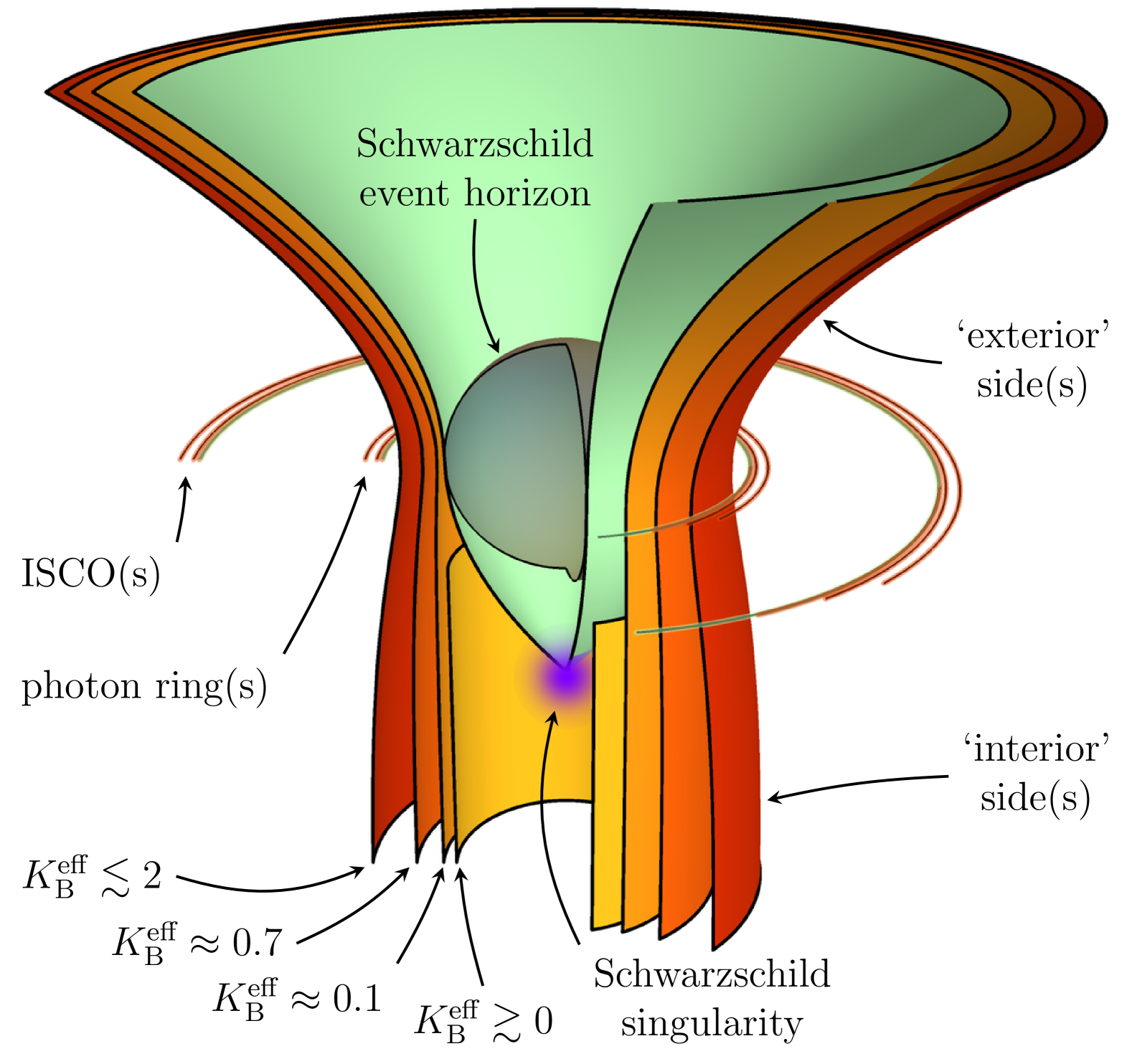
Figure 1: Embedding visualisation of spatial geometry. Black hole mimickers in æther-scalar-tensor theory (orange/red, see Eqs. 2, 3 and 4) emulate the Schwarzschild geometry (green, see Eq. 1) with the same Newtonian mass $M$, but have slightly dilated features and a narrow wormhole throat instead of an event horizon. An alternative horizon lies on the ‘interior’ side (here truncated).

Black hole mimickers

We propose the BH mimicker of ÆST to be a highly asymmetric wormhole, leading only to a BH-type object on its ‘interior’ side. To keep our key results within in this opening section, we quote here our predicted line element on the ‘exterior’ side, i.e. that which is most relevant to observations. For reference, in GR with Newton–Cavendish constant $G$, the Schwarzschild BH of mass $M$ is described by

$$\mathrm{d}s^{2}=-\left(1-\tfrac{2GM}{r}\right)\mathrm{d}t^{2}+\frac{\mathrm{d}r^{2}}{\left(1-\tfrac{2GM}{r}\right)}+r^{2}\,\mathrm{d}\Omega^{2}\,\,,$$ (1)

where $\mathrm{d}\Omega^{2}\equiv\mathrm{d}\theta^{2}+\sin^{2}(\theta)\mathrm{d}\phi^{2}$ is the angular measure. The ‘exterior’ side of our mimicker generalises Eq. 1 to

$$\mathrm{d}s^{2}=-e^{2\mathcal{N}(r)}\,\mathrm{d}t^{2}+e^{2\mathcal{M}(r)}\,\mathrm{d}r^{2}+r^{2}\,\mathrm{d}\Omega^{2}.$$ (2)

Whilst Eq. 1 would imply $\mathcal{N}(r)=-\mathcal{M}(r)$, the BH mimicker instead requires the cumbersome relation

$$e^{2\mathcal{N}(r)} =\left[\frac{\sqrt{2}-\sqrt{2-\tensor{*}{K}{{}_{\text{B}}^{\text{eff}}}}}{\sqrt{2}+\sqrt{2-\tensor{*}{K}{{}_{\text{B}}^{\text{eff}}}}}\right.$$ (3)

$$\hskip-30.0pt\times\left.\frac{\sqrt{2+\tensor{*}{K}{{}_{\text{B}}^{\text{eff}}}(e^{2\mathcal{M}(r)}-1)}-\sqrt{2-\tensor{*}{K}{{}_{\text{B}}^{\text{eff}}}}}{\sqrt{2+\tensor{*}{K}{{}_{\text{B}}^{\text{eff}}}(e^{2\mathcal{M}(r)}-1)}+\sqrt{2-\tensor{*}{K}{{}_{\text{B}}^{\text{eff}}}}}\right]^{\sqrt{\frac{2}{2-\tensor{*}{K}{{}_{\text{B}}^{\text{eff}}}}}}.$$

The formula in Eq. 3 depends strongly on the dimensionless parameter $\tensor{*}{K}{{}_{\text{B}}^{\text{eff}}}{}<2$. For the moment, it suffices to know that $\tensor{*}{K}{{}_{\text{B}}^{\text{eff}}}{}$ depends on (i) two of the constant ÆST model parameters and (ii) some dynamically acquired flux of scalar hair. The actual formula for $\mathcal{M}(r)$ is defined as being the inverse of an ‘$r\left(\mathcal{M}\right)$’ formula

$$\hskip-5.0ptr=\frac{\tensor{*}{G}{{}_{\text{N}}}M\tensor{*}{K}{{}_{\text{B}}^{\text{eff}}}e^{\mathcal{M}(r)}}{\sqrt{4+2\tensor{*}{K}{{}_{\text{B}}^{\text{eff}}}\left(e^{2\mathcal{M}(r)}-1\right)}-2}\left[\frac{\sqrt{2}+\sqrt{2-\tensor{*}{K}{{}_{\text{B}}^{\text{eff}}}}}{\sqrt{2}-\sqrt{2-\tensor{*}{K}{{}_{\text{B}}^{\text{eff}}}}}\right.$$ (4)

$$\hskip-10.0pt\times\left.\frac{\sqrt{2+\tensor{*}{K}{{}_{\text{B}}^{\text{eff}}}\left(e^{2\mathcal{M}(r)}-1\right)}-\sqrt{2-\tensor{*}{K}{{}_{\text{B}}^{\text{eff}}}}}{\sqrt{2+\tensor{*}{K}{{}_{\text{B}}^{\text{eff}}}\left(e^{2\mathcal{M}(r)}-1\right)}+\sqrt{2-\tensor{*}{K}{{}_{\text{B}}^{\text{eff}}}}}\right]^{\frac{\tensor{*}{K}{{}_{\text{B}}^{\text{eff}}}{}}{2\tensor{*}{K}{{}_{\text{B}}^{\text{eff}}}{}-4+2\sqrt{4-2\tensor{*}{K}{{}_{\text{B}}^{\text{eff}}}}}}\hskip-50.0pt,$$

where the Newtonian $\tensor{*}{G}{{}_{\text{N}}}{}$ in Eq. 3 is also shifted relative to the bare $G$ in Eq. 1 by ÆST model parameters. The take-home point is that Eqs. 2, 3 and 4 ‘mimick’ Eq. 1 to arbitrary precision as $\tensor{*}{K}{{}_{\text{B}}^{\text{eff}}}{}\to 0$. This is illustrated in Fig. 1, which shows a faithful embedding of 2D equatorial constant-time slices in 3D space. Where the Schwarzschild geometry has an event horizon, however, the BH mimicker always has a slight throat, on the ‘interior’ side of which lies a null singularity. We imagine BH mimickers as accounting for some clandestine fraction of the observed BH population. They would presumably evade all radio, astrometric and GW bounds on the external geometry, and all optical, X-ray and GW bounds on surface characteristics. Signals for BH mimickers from ÆST may include (i) corrections to radio imaging within the photon ring from ‘interior’-side emissions, and (ii) non-BH ringdown.

Confidence in lenses

We will also be interested in hard-to-find exotic objects that do not mimick BHs, but whose subtle lensing properties would provide a smoking gun for ÆST (see Fig. 2) [32, 33]. Statistical microlensing campaigns (MACHO, EROS, OGLE) constrain the fraction of compact lenses in galactic halos across ${10}^{-7}\text{\,}\mathrm{M_{\odot}}10\text{\,}\mathrm{M_{\odot}}$ to below a few percent of CDM [34, 35], while forthcoming wide‐field surveys (LSST) will extend sensitivity to sub-lunar masses [36, 37]. Pulsar timing constrains populations of exotic lenses which have become entrained in binary systems. Precision monitoring of binary pulsars — most notably the Hulse–Taylor and subsequent millisecond systems — has confirmed the Shapiro delay (lensing in time) predicted by GR to sub-percent accuracy [38, 39]. No anomalous timing residuals attributable to scalar charges or exotic multipole structure have been observed in existing systems [40, 41]. Pulsar timing arrays (NANOGrav, EPTA, PPTA) likewise report a stochastic background consistent with a population of supermassive BH binaries and show no non-quadrupolar radiation or unexpected spectral features [42, 43]. Notice, however, how all these constraints presume CDM-type lenses, which ‘weigh’ and thus participate in Newtonian gravity. Recalling, therefore, that we have no need of dark matter candidates in ÆST, this motivates considering an extreme case: a ‘weightless’ gravitational lens.

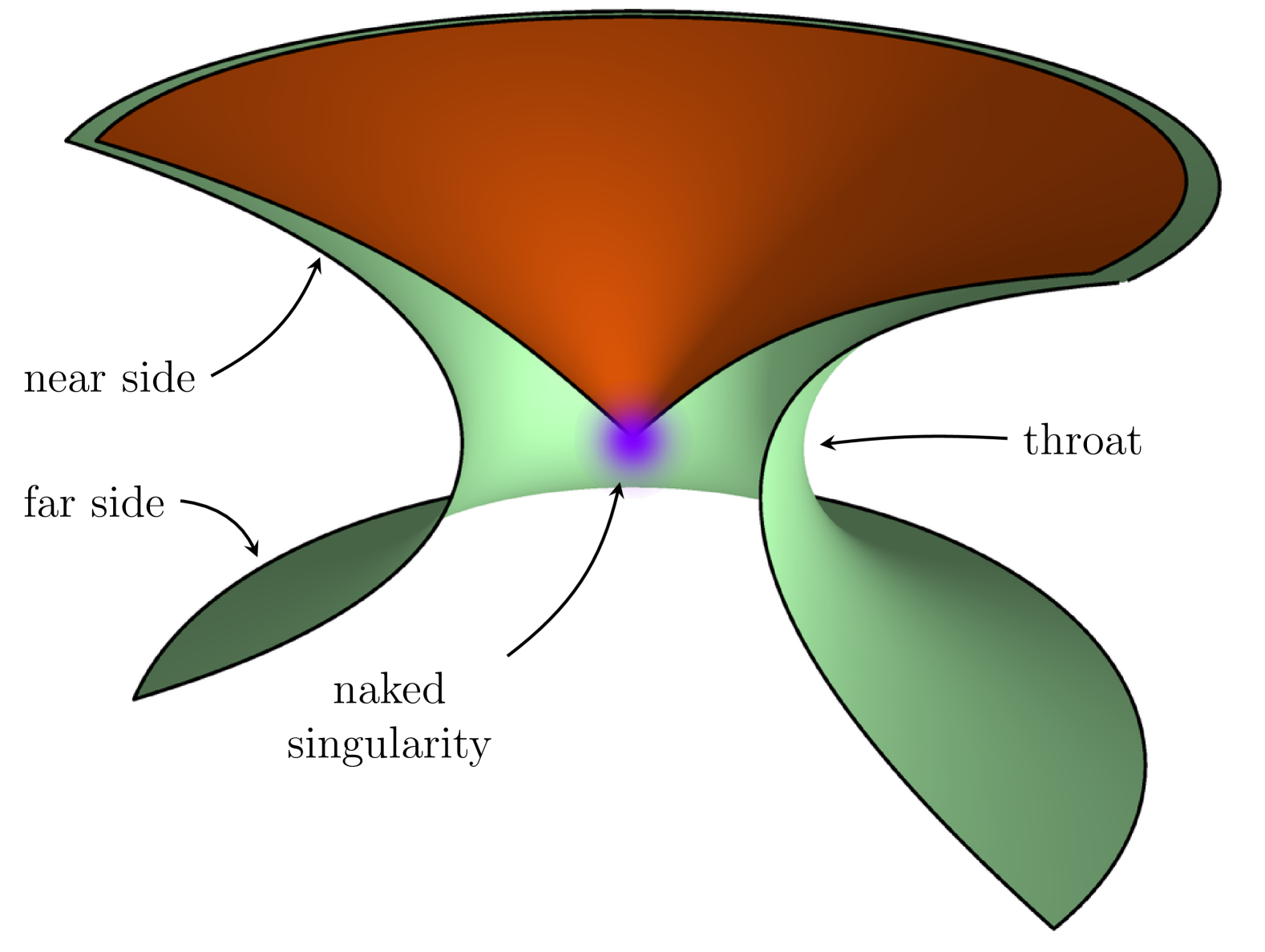
Figure 2: Embedding visualisation of spatial geometry. Lenses without Shapiro delay in æther-scalar-tensor theory (red, see ‘$(-)$’ configuration in Eq. 5) are massless regions of curved space ending in a naked singularity. They are the analytic continuation of Ellis wormholes (green, see ‘$(+)$’ configuration in Eq. 5).

Shapiro-free lenses

We propose a ‘weightless’ lens in ÆST, inspired by the massless Ellis–Bronnikov wormhole [44, 45] as given by the ‘$(+)$’ configuration in

$$\mathrm{d}s^{2}=-\mathrm{d}t^{2}+\mathrm{d}r^{2}+\left(r^{2}\mp\ell^{2}\right)\mathrm{d}\Omega^{2}\,\,,$$ (5)

where $t$ and $r$ are now the proper time and radius. As popularised by Visser [46, 47], Morris and Thorne [48, 49], the ‘$(+)$’ configuration is a far less subtle wormhole than the BH mimicker, with correspondingly more applications in science fiction: it seemingly allows test geodesics to pass between two asymptotically flat regions via a ‘throat’ of minimal area $4\pi\ell^{2}$ at $r=0$, which needs to be held open by phantom matter in the Einstein field equations. By contrast, the ‘$(-)$’ configuration of Eq. 5 requires no phantom matter, being an exact solution to the ÆST field equations in which the wormhole throat closes up. This promotes the object from a formal curiosity to a subtle observational challenge. Its constant-time hypersurfaces are highly curved, as illustrated in Fig. 2 — indeed this figure captures the full Riemannian curvature, which has no ‘time part’ whatever (so-called ultrastaticity). The object thus has no mass $M$ at infinity, no gravitational redshift, and indeed no gravity. A naked singularity (or star-like matter configuration) sources the scalar hair and sets $\ell$, but it does not accrete, and whilst its spatial curvature gives rise to lensing, the lensed rays experience no Shapiro delay. The object is also more compact than its Schwarzschild equivalent in Eq. 1, and optically repulsive; its spatial lensing potential scales as $\sim 1/r^{2}$ rather than $\sim 1/r$, and has the opposite sign, akin to negative mass in GR. A population of such lenses (e.g. early-Universe relics) would seem hard — but not impossible — to observe, providing a clear signal for ÆST.

In this work

Our objective is to show that (i) the exact solutions proposed in Eqs. 2, 3, 4 and 5 do indeed satisfy the ÆST field equations, and (ii) that they have the above phenomenological properties. Two aspects need to be investigated in further work. Firstly, dynamical production and stability against perturbations, in the context of cosmological/astrophysical backgrounds and timescales, leading to abundance predictions. Secondly, computation of precise observational signatures leading to multi-messenger forecasts. In Section II.3 we will obtain the field equations of ÆST. In Section III we obtain the compact solutions, with a cosmological solution in Section IV. We conclude in Section V. Technical appendices follow, including two of general interest. In Appendix C, we show that the acceleration of static æther is generally a conserved current. In Appendix E we show that the BH mimicker is a wormhole in name only: instead of leading to another universe, it leads to a singular Killing horizon.

Conventions

We try to match [10, 50], using the signature $(-,+,+,+)$, and natural units $c\equiv\hbar\equiv 1$. Further conventions are introduced as needed.

II Theoretical development

II.1 Overview of theories

Scalar-tensor theory

The simplest extension of GR is the massless scalar-tensor theory

$$\tensor{*}{S}{{}_{\text{ST}}}\equiv\int\mathrm{d}^{4}x\,\frac{\sqrt{-g}}{2\kappa}\bigg{[}R\mp\tensor{\nabla}{{}_{\mu}}\varphi\tensor{\nabla}{{}^{\mu}}\varphi\bigg{]},$$ (6)

where $R$ is the Ricci scalar, and $\kappa\equiv 8\pi G$ is the Einstein constant with $G$ the Newton–Cavendish constant. The shift-symmetric scalar $\varphi$ is made dimensionless in Eq. 6, and with our signature the ‘$(\mp)$’ sign allows canonical ‘$(-)$’ or phantom ‘$(+)$’ character. One of our key findings will be that this primitive class of models goes a long way towards explaining the solutions of ÆST, even though the latter is a far more intricate model. This is especially surprising, because whilst ÆST also contains a shift-symmetric scalar $\varphi$, the operators of this field are everywhere entangled with an additional dimensionless vector field $\tensor{A}{{}^{\mu}}$, which has an æther character.

Einstein-æther theory

By contrast with the scalar-tensor theory of Eq. 6, the simplest æther model is Maxwell-type Einstein-æther (EÆ) theory [51, 52]. The action, using $\tensor{F}{{}_{\mu}{}_{\nu}}\equiv\tensor{\nabla}{{}_{\mu}}\tensor{A}{{}_{\nu}}-\tensor{\nabla}{{}_{\nu}}\tensor{A}{{}_{\mu}}$, is given by

$$\tensor{*}{S}{{}_{\text{E\AE {}}}} \equiv\int\mathrm{d}^{4}x\,\frac{\sqrt{-g}}{2\kappa}\Bigg{[}R-\frac{\tensor{K}{{}_{\text{B}}}{}}{2}\tensor{F}{{}^{\mu\nu}}\tensor{F}{{}_{\mu\nu}}$$ (7)

$$\hskip 80.0pt-\lambda\left(\tensor{A}{{}^{\mu}}\tensor{A}{{}_{\mu}}+1\right)\Bigg{]},$$

where the dimensionless æther coupling lies in the range

$$0<\tensor{K}{{}_{\text{B}}}{}<2\,\,,$$ (8)

mandated by the stability of perturbations. The general idea is to identify a preferred frame at each point in the spacetime as having a four-velocity given by the vector field $\tensor{A}{{}^{\mu}}$. For this interpretation to hold, the vector must be everywhere timelike and with unit length: these conditions are ensured in Eq. 7 by the dynamics of $\lambda$, which is a Lagrange multiplier. Ignoring the multiplier terms leads back to Einstein–Maxwell theory in which $\sqrt{\tensor{K}{{}_{\text{B}}}{}/\kappa}\tensor{A}{{}^{\mu}}$ is the electromagnetic gauge potential.

Æther-scalar-tensor theory

Going beyond scalar-tensor and EÆ theories, ÆST blends the dynamics of $\varphi$ and $\tensor{A}{{}^{\mu}}$ through the action

$$\tensor{*}{S}{{}_{\text{\AE {}ST}}} \equiv\int\mathrm{d}^{4}x\,\frac{\sqrt{-g}}{2\kappa}\Bigg{[}R-\frac{\tensor{K}{{}_{\text{B}}}{}}{2}\tensor{F}{{}^{\mu\nu}}\tensor{F}{{}_{\mu\nu}}$$ (9)

$$\hskip 30.0pt+2\left(2-\tensor{K}{{}_{\text{B}}}{}\right)\tensor{J}{{}^{\mu}}\tensor{\nabla}{{}_{\mu}}\varphi-\left(2-\tensor{K}{{}_{\text{B}}}{}\right)\mathcal{Y}$$

$$\hskip 30.0pt-\mathcal{F}\left(\mathcal{Y},\mathcal{Q}\right)-\lambda\left(\tensor{A}{{}^{\mu}}\tensor{A}{{}_{\mu}}+1\right)\Bigg{]}\,\,,$$

where, as in EÆ theory, we assume Eq. 8 for reasons of stability [53]; the other quantities in Eq. 9 are defined

$$\begin{gathered}\tensor{J}{{}_{\mu}}\equiv\tensor{A}{{}^{\nu}}\tensor{\nabla}{{}_{\nu}}\tensor{A}{{}_{\mu}},\quad\tensor{q}{{}_{\mu}{}_{\nu}}\equiv\tensor{g}{{}_{\mu}{}_{\nu}}+\tensor{A}{{}_{\mu}}\tensor{A}{{}_{\nu}},\\ \mathcal{Q}\equiv\tensor{A}{{}^{\mu}}\tensor{\nabla}{{}_{\mu}}\varphi,\quad\mathcal{Y}\equiv\tensor{q}{{}^{\mu}{}^{\nu}}\tensor{\nabla}{{}_{\mu}}\varphi\tensor{\nabla}{{}_{\nu}}\varphi.\end{gathered}$$ (10)

In particular, if $\tensor{A}{{}^{\mu}}$ is interpreted as the four-velocity of the preferred frame, then it follows from Eq. 10 that $\tensor{J}{{}^{\mu}}$ must be the four-acceleration of that frame. In general, $\mathcal{F}(\mathcal{Y},\mathcal{Q})$ is a free function of the scalars $\mathcal{Y}$ and $\mathcal{Q}$. One motivated form for this function was proposed in [10], whereby

$$\mathcal{F}(\mathcal{Y},\mathcal{Q})=\left(2-\tensor{K}{{}_{\text{B}}}{}\right)\mathcal{J}\left(\mathcal{Y}\right)-\mathcal{F}_{20}\left(\mathcal{Q}-\mathcal{Q}_{0}\right)^{2}\,,$$ (11)

where $\mathcal{Q}_{0}$ has mass-dimension one and

$$\mathcal{F}_{20}>0,$$ (12)

is dimensionless. The idea behind Eq. 11 is that the $\mathcal{Q}$-dependent term is responsible for reproducing a cosmological CDM-like component, while the $\mathcal{Y}$-dependent term is responsible for explaining the missing mass problem in galaxies [10]. Heuristically, $\mathcal{Q}$ carries the time derivatives of the scalar field, while $\mathcal{Y}$ carries the spatial derivatives, so that $\mathcal{Q}$ is relevant in time-dependent situations (e.g. cosmology) while $\mathcal{Y}$ is relevant to static or quasi-static situations (e.g. galaxies). To reproduce the successes of MOND in describing gravity on galactic scales, the function $\mathcal{J}(\mathcal{Y})$ in Eq. 11 is (somewhat hazily) defined as

$$\mathcal{J}\left(\mathcal{Y}\right)\equiv\begin{cases}\lambda_{s}\mathcal{Y},\quad&\mathcal{J}(\mathcal{Y})\gg a_{0}^{2},\\ \frac{2\lambda_{s}\mathcal{Y}^{3/2}}{3\left(1+\lambda_{s}\right)a_{0}},\quad&\mathcal{J}(\mathcal{Y})\ll a_{0}^{2},\end{cases}$$ (13)

where $a_{0}\sim$1\text{\times}{10}^{-10}\text{\,}\mathrm{m}\text{\,}{\mathrm{s}}^{-2}$$ is the MOND acceleration scale, and the dimensionless parameter $\lambda_{s}$ obeys

$$1<\lambda_{s},$$ (14)

again to avoid an instability [53]. In galaxies, Eq. 13 will reproduce Newtonian gravity at accelerations large compared to $a_{0}$, and MOND-like gravity at accelerations small compared to $a_{0}$. In the following we will mostly restrict ourselves to the Newtonian ansatz for $\mathcal{J}\left(\mathcal{Y}\right)$, which is relevant to small radii, appropriate for BH and wormhole solutions. Without introducing new parameters to modify the Newtonian ansatz, we will find that the strong-field departures from Newtonian phenomena have remarkably promising observational implications. Having already restricted to the minimal quadratic $\mathcal{Q}$ ansatz required for effective CDM, our decision to neglect the MOND ansatz allows us to avoid the further set of arbitrarily many parameters that would interpolate between the two ansätze for $\mathcal{J}\left(\mathcal{Y}\right)$. Even with this maximally predictive approach, the prior constraints on the five remaining parameters in ÆST, namely $G$, $\tensor{K}{{}_{\text{B}}}{}$, $\lambda_{s}$, $\mathcal{F}_{20}$ and $\mathcal{Q}_{0}$, remain very weak. They include

$$\frac{2\left(1+\lambda_{s}\right)}{\lambda_{s}\left(2-\tensor{K}{{}_{\text{B}}}{}\right)}\mathcal{F}_{20}\mathcal{Q}_{0}^{2}\sim$1\text{\,}{\mathrm{Mpc}}^{-2}$\,\,,$$ (15)

which was arrived at in [11] as a ‘goldilocks’ estimate for producing MOND in galaxies, and suppressing it on the scale of galaxy clusters (see also [54]). An extra subtlety also affects $G$ (i.e. $\kappa$) in Eq. 9, which in ÆST should be considered a bare coupling. The measured Newtonian $\tensor{*}{G}{{}_{\text{N}}}{}\approx$6.67\text{\times}{10}^{-11}\text{\,}{\mathrm{m}}^{3}\text{\,}{\mathrm{kg}}^{-1}\text{\,}{\mathrm{s}}^{-2}$$ was derived in [10], and found to be given by the formula

$$\tensor{*}{G}{{}_{\text{N}}}{}\equiv\frac{\left(1+\lambda_{s}\right)2G}{\lambda_{s}\left(2-\tensor{K}{{}_{\text{B}}}{}\right)}\,\,,$$ (16)

where $G$, $\tensor{K}{{}_{\text{B}}}{}$ and $\lambda_{s}$ are otherwise unconstrained.

II.2 Relevant solutions

Ellis–Bronnikov drainhole

Solutions in scalar-tensor theory have been extensively studied [55, 56, 57]. The phantom ‘$(+)$’ case of Eq. 6 admits the celebrated two-parameter ‘drainhole’ solution of Ellis [44] and Bronnikov [45] (see also [56, 57, 58, 59]). Both sides of this asymmetric wormhole are asymptotically flat. The near side behaves like the Schwarzschild solution at spatial infinity, one of the parameters setting the attractive asymptotic mass; the far side is correspondingly repulsive. The throat of the wormhole is independently dilated by the second parameter. The massless limit is a symmetric, one-parameter wormhole. The absence of a mass means that, throughout the whole spacetime, static observers experience no acceleration. The resulting wormhole has no gravity, and geodesics ‘coast’ freely from one side to the other only if they happen to intersect the throat.

Fisher–JNW solution

Conversely, if the scalar is canonical, i.e. the ‘$(-)$’ case of Eq. 6, there is a two-parameter analogue of the Ellis–Bronnikov solution attributed first to Fisher [60] and rediscovered much later by Janis, Newman and Winicour (JNW) [61]. The analogy is exact, in the sense that analytic continuation of the Fisher–JNW solution to the phantom ‘$(+)$’ case just yields the Ellis–Bronnikov drainhole in different coordinates. Non-phantom Fisher–JNW spacetime is also asymptotically flat, but it contains a naked singularity at its centre, not a throat. As with the Ellis–Bronnikov solution, however, there exists a massless limit: the naked singularity persists, but it is weightless, so that static observers are not drawn towards it.

Eling–Jacobson wormhole

Static, spherical solutions to EÆ theory in Eq. 7 were studied extensively by Eling and Jacobson in [62]. The Eling–Jacobson solution is also massive, with an asymptotically flat near side (which we will think of as an ‘exterior’) consistent with the Newtonian limit of the Schwarzschild solution. The Eling–Jacobson solution, however, does not quite describe a BH, but rather a highly asymmetric wormhole. On the far side (‘interior’) of its throat lies a very different region which is not asymptotically flat, but which ends at a singular Killing horizon. In the $\tensor{K}{{}_{\text{B}}}{}\to 0$ limit, the throat radius approaches (from above) the value of the Schwarzschild radius associated with the mass, and in fact the whole ‘exterior’-side geometry approaches the Schwarzschild vacuum.

Stealth BH

Ignoring the multiplier term in Eq. 7 yields Einstein–Maxwell theory. It is sometimes forgotten that a unit-timelike condition on the electromagnetic gauge potential is actually a perfectly valid gauge choice in electromagnetism. Indeed, this Dirac gauge was among the earliest motivations for æther models such as the EÆ theory. It is unsurprising, therefore, that one branch of solutions to EÆ theory is actually Reissner–Nordström. Less obvious is the fact that this solution is also inherited by ÆST, as shown recently in [14]. In the limit of vanishing charge, the Reissner–Nordström geometry cannot be observationally distinguished from that of Schwarzschild, and such field configurations in ÆST have been dubbed ‘stealth’ BHs.

II.3 Overview of equations

Simplified action

Our starting point for everything that follows will be to refine Eq. 9 by assuming the form proposed by Skordis and Złosnik in Eq. 11. We will not, however, enforce the assumptions in Eq. 13, which lead to MOND phenomenology. We rewrite the action as

$$\tensor{*}{S}{{}_{\text{\AE {}ST}}^{\text{SZ}}} \equiv\int\mathrm{d}^{4}x\,\frac{\sqrt{-g}}{2\kappa}\Bigg{[}{R}-\frac{\tensor{K}{{}_{\text{B}}}{}}{2}\tensor{F}{{}^{\mu\nu}}\tensor{F}{{}_{\mu\nu}}$$ (17)

$$\hskip 20.0pt+2\left(2-\tensor{K}{{}_{\text{B}}}{}\right)\tensor{J}{{}^{\mu}}\tensor{\nabla}{{}_{\mu}}\varphi-\mathcal{V}\left(\mathcal{Y}\right)$$

$$\hskip 20.0pt+\mathcal{F}_{20}\left(\mathcal{Q}-\mathcal{Q}_{0}\right)^{2}-\lambda\left(\tensor{A}{{}^{\mu}}\tensor{A}{{}_{\mu}}+1\right)\Bigg{]}\,\,,$$

so that $\mathcal{J}(\mathcal{Y})$ from Eq. 11 and $(2-\tensor{K}{{}_{\text{B}}}{})\mathcal{Y}$ from Eq. 9 are combined into the ‘potential’ $\mathcal{V}(\mathcal{Y})$.

Covariant equations

The field equations are obtained by taking variations of Eq. 17 with respect to the dynamical degrees of freedom: the metric $\tensor{g}{{}_{\mu\nu}}$, the æther field $\tensor{A}{{}^{\mu}}$, the scalar field $\varphi$ and the Lagrange multiplier $\lambda$. Variation with respect to $\lambda$ yields the normalization constraint on the æther field

$$\tensor{A}{{}^{\mu}}\tensor{A}{{}_{\mu}}=-1\,\,.$$ (18)

Even after Eq. 18 has been imposed, the remaining field equations (which include among their components propagating equations as well as constraints) remain somewhat cumbersome, and we confine them to Appendix A. Note that the $A^{\mu}$-equation contains a term of the form $\delta\tensor{*}{S}{{}_{\text{\AE {}ST}}^{\text{SZ}}}/\delta\tensor{A}{{}^{\mu}}\supset-\sqrt{-g}\lambda\tensor{A}{{}_{\mu}}/\kappa$, so that after contraction with an extra factor of $A^{\mu}$ followed by an application of Eq. 18 it allows for the Lagrange multiplier $\lambda$ to be determined algebraically (see Eq. 66).

Component equations

Initially, the line element in the spherically symmetric spacetime is not assumed to be Schwarzschild-like or isotropic; we write

$$\mathrm{d}s^{2}=-e^{2\mathcal{N}(r)}\,\mathrm{d}t^{2}+e^{2\mathcal{M}(r)}\,\mathrm{d}r^{2}+\mathcal{R}(r)^{2}\,\mathrm{d}\Omega^{2}\,\,,$$ (19)

and this provides our ansatz for the metric $\tensor{g}{{}_{\mu\nu}}$. The scalar field $\varphi$ and the æther field $\tensor{A}{{}^{\mu}}$ are assumed to share the same spherical symmetry with the spacetime. In the case of the æther field, this means that only temporally and radially aligned components are allowed, and together with Eqs. 18 and 19 this yields

$$\left[\tensor{A}{{}_{\mu}}\right]=\left[\cosh\big{(}\alpha(r)\big{)}e^{\mathcal{N}(r)},\sinh\big{(}\alpha(r)\big{)}e^{\mathcal{M}(r)},0,0\right].$$ (20)

Finally, we allow $\varphi$ to additionally have some time dependence, which is related to the first term in Eq. 11

$$\varphi=\mathcal{Q}_{0}\chi(t)+\psi(r),$$ (21)

accordingly, we refer to it as $\varphi(t,r)$. The component-level equations following from Eqs. 19, 20 and 21 can be found in Appendix B. From this point on, however, we will focus on the solutions with purely time-aligned æther (the so-called ‘static æther’ condition), by setting

$$\alpha(r)=0,$$ (22)

in Eq. 19. Following from Eq. 22 we then find (see discussion in Appendix C)

$$\begin{gathered}\tensor{F}{{}_{\mu\nu}}\tensor{F}{{}^{\mu\nu}}=-2\tensor{J}{{}_{\mu}}\tensor{J}{{}^{\mu}},\quad\tensor{J}{{}_{\mu}}\tensor{\nabla}{{}^{\mu}}\varphi=\tensor{J}{{}_{\mu}}\tensor{\nabla}{{}^{\mu}}\psi,\\ \mathcal{Y}=\tensor{\nabla}{{}_{\mu}}\psi\,\tensor{\nabla}{{}^{\mu}}\psi,\quad\mathcal{Q}=-\mathcal{Q}_{0}\frac{\mathrm{d}\chi}{\mathrm{d}t}e^{-\mathcal{N}}.\end{gathered}$$ (23)

We will also impose the constraint on Eq. 19

$$\mathcal{M}(r)=-\mathcal{N}(r)\,.$$ (24)

The condition in Eq. 24 can always be met by a suitable rescaling of $r$. In general, this choice will not coincide with $\mathcal{R}(r)=r^{2}$. Accordingly, $r$ need not be tied to the area of enclosing two-spheres, so the resulting coordinates need not be Schwarzschild-like. Note, however, that in general, the $r$ coordinate scaled according to Eqs. 19 and 24 is proportional to the affine parameter of radial null geodesics. When Eqs. 22, 21 and 24 are imposed on the field equations, a constraint from Eq. 67b yields (see Appendix D)

$$\mathcal{Q}_{0}\Bigg{(} \left[\left(2-\tensor{K}{{}_{\text{B}}}{}\right)\frac{{\mathrm{d}}\mathcal{N}}{{\mathrm{d}}r}+\left(\mathcal{F}_{20}-\frac{{\mathrm{d}}\mathcal{V}}{{\mathrm{d}}\mathcal{Y}}\right)\frac{{\mathrm{d}}\psi}{{\mathrm{d}}r}\right]\frac{{\mathrm{d}}\chi}{{\mathrm{d}}t}$$ (25)

$$\hskip 110.0pt-\mathcal{F}_{20}e^{\mathcal{N}}\frac{{\mathrm{d}}\psi}{{\mathrm{d}}r}\Bigg{)}=0,$$

and Eq. 25 will be instrumental in guiding our search for solutions. We will show that the spherically symmetric, static solutions to the ÆST field equations can have both scalar-tensor and EÆ character. In particular, we show that ÆST in Eq. 9 inherits the Eling–Jacobson wormhole of EÆ theory in Eq. 7, but with an ‘effective’ æther coupling $\tensor{*}{K}{{}_{\text{B}}^{\text{eff}}}{}$, which is shifted relative to the bare $\tensor{K}{{}_{\text{B}}}{}$ by the scalar current. This solution forms the basis for our BH mimicker. We will uncover a second branch of solutions for which the æther acceleration $\tensor{J}{{}^{\mu}}$ vanishes: this describes an ultrastatic (massless) spacetime, and forms the basis for our Shapiro-free lens.

III Asymptotically flat cases

Guiding equations

To obtain asymptotically flat solutions, we need to neglect the MOND regime. Without MOND, by referring to Eq. 13 we see that the function $\mathcal{V}(\mathcal{Y})$ in Eq. 17 is linear, i.e.

$$\mathcal{V}(\mathcal{Y})=\left(2-\tensor{K}{{}_{\text{B}}}{}\right)\left(1+\lambda_{s}\right)\mathcal{Y}.$$ (26)

Our discussion will be driven in particular by two component-level conditions that arise out of the field equations when the assumptions in Eqs. 22, 21, 24 and 26 are applied. Firstly, is found that Eq. 67e provides a necessary condition for the existence of non-trivial solutions

$$\mathcal{F}_{20}\mathcal{Q}_{0}\mathcal{R}\frac{\mathrm{d}\psi}{\mathrm{d}r}\left(e^{\mathcal{N}}-\frac{\mathrm{d}\chi}{\mathrm{d}t}\right)=0\,\,.$$ (27)

We focus on the case where Eq. 27 is satisfied because

$$\mathcal{F}_{20}\mathcal{Q}_{0}=0.$$ (28)

Referring back to Eq. 11, the condition in Eq. 28 implies that we are neglecting the capacity of ÆST to provide a CDM component in the cosmological background and perturbation theory — again, this ought to be safe for strong fields. Secondly, under Eqs. 28 and 26 the complicated constraint in Eq. 25 reduces to

$$\mathcal{Q}_{0}\frac{\mathrm{d}\chi}{\mathrm{d}t}\left(\frac{\mathrm{d}\mathcal{N}}{\mathrm{d}r}-\left(1+\lambda_{s}\right)\frac{\mathrm{d}\psi}{\mathrm{d}r}\right)=0,$$ (29)

which has a much simpler form.

Heuristic action

When Eqs. 19, 20, 21, 22, 28 and 26 hold, Eq. 23 can be used to re-write the action in Eq. 17 as

$$\tensor{*}{S}{{}_{\text{\AE {}ST}}^{\text{SZ}}}\cong\int\mathrm{d}^{4}x\,\frac{\sqrt{-g}}{2\kappa}\Big{[}R+{\tensor{K}{{}_{\text{B}}}{}}\tensor{J}{{}^{\mu}}\tensor{J}{{}_{\mu}}-\lambda\left(\tensor{A}{{}^{\mu}}\tensor{A}{{}_{\mu}}+1\right)$$

$$\hskip 35.0pt+\left(2-\tensor{K}{{}_{\text{B}}}{}\right)\Big{(}2\tensor{J}{{}^{\mu}}-\left(1+\lambda_{s}\right)\tensor{\nabla}{{}^{\mu}}\psi\Big{)}\tensor{\nabla}{{}_{\mu}}\psi\Big{]}.$$ (30)

We have verified explicitly that the equations of motion derived from Eq. 30 reproduce the solutions of the original action in Eq. 17, expressed in terms of the metric $g_{\mu\nu}$, the scalar $\varphi$, and the vector $A^{\mu}$, after Eqs. 19, 20, 21, 22, 28 and 26 are imposed. We particularly notice in Eq. 30 that all $\chi(t)$ dependence has disappeared. This is because the ‘acceleration’ of the æther defined in Eq. 10 has only one non-vanishing component $J_{r}=\mathrm{d}\mathcal{N}/\mathrm{d}r$, whilst $q^{tt}$ vanishes due to Eq. 22. The absence of $\chi(t)$ will be exploited in Section III.2. From Eq. 30, the field equation associated with the one remaining scalar $\psi(r)$ takes the form of a conservation law

$$\tensor{\nabla}{{}_{\mu}}\big{(}\tensor{J}{{}^{\mu}}-\left(1+\lambda_{s}\right)\tensor{\nabla}{{}^{\mu}}\psi\big{)}=0\,\,,$$ (31)

which reflects the surviving shift symmetry.

Possible branches

There are evidently at least two ways to realize Eq. 28, $\mathcal{Q}_{0}=0$ and $\mathcal{F}_{20}=0$. Perhaps surprisingly, the $\mathcal{F}_{20}(\mathcal{Q}-\mathcal{Q}_{0})^{2}$ term in Eq. 17 is absent from Eq. 30 not just in the case $\mathcal{F}_{20}=0$ but also for $\mathcal{Q}_{0}=0$. This is because the condition $\mathcal{Q}_{0}=0$ is not only a statement about the constants parameterizing the action in Eq. 17, but also about the scalar field in Eq. 21. In particular, it eliminates all time dependence in $\varphi$, so that Eq. 23 leads to $\mathcal{Q}$ vanishing identically, along with $\mathcal{F}_{20}(\mathcal{Q}-\mathcal{Q}_{0})^{2}$. Despite the action in Eq. 30 having the same form for $\mathcal{F}_{20}=0$ and $\mathcal{Q}_{0}=0$, the solutions in either case are not identical, as we will see below.

III.1 New branches of exact solutions

General case

The first realisation of Eq. 28 will be through the condition

$$\mathcal{F}_{20}\neq 0,\quad\mathcal{Q}_{0}=0\,.$$ (32)

In this case, we satisfy Eq. 29 by assuming no time dependence in $\varphi(t,r)$, so that Eq. 21 implies simply

$$\chi(t)=0\,.$$ (33)

The crucial point is that the reduced covariant action for ÆST in Eq. 30 reduces to the corresponding action for EÆ theory in Eq. 7 if $\tensor{\nabla}{{}_{\mu}}\psi$ is proportional to $\tensor{J}{{}_{\mu}}$. For example, if

$$\tensor{\nabla}{{}_{\mu}}\psi=q\tensor{J}{{}_{\mu}},$$ (34)

for some constant $q$, then Eq. 30 reduces to Eq. 7 in which $\tensor{K}{{}_{\text{B}}}{}$ is replaced by an ‘effective’ æther coupling

$$\tensor{*}{K}{{}_{\text{B}}^{\text{eff}}}{}\equiv\tensor{K}{{}_{\text{B}}}{}+\left(2-\tensor{K}{{}_{\text{B}}}{}\right)q\Big{[}2-\left(1+\lambda_{s}\right)q\Big{]}\,\,.$$ (35)

This raises the possibility of ‘lifting’ solutions from the original EÆ theory to ÆST. In component form, the condition in Eq. 34 implies

$$\frac{\mathrm{d}\psi}{\mathrm{d}r}=q\frac{\mathrm{d}\mathcal{N}}{\mathrm{d}r},$$ (36)

but Eq. 36 is not the only condition on $\psi(r)$. It is shown in Appendix C that for static æther in static geometries which solve the EÆ field equations, one always has the identity

$$\tensor{\nabla}{{}_{\mu}}\tensor{J}{{}^{\mu}}=0.$$ (37)

If Eq. 37 holds, then Eq. 31 requires that the scalar field must satisfy the massless Klein–Gordon equation

$$\tensor{\nabla}{{}_{\mu}}\tensor{\nabla}{{}^{\mu}}\,\psi=0\,.$$ (38)

We reiterate that the reason for suppressing time dependence in Eq. 33 is that otherwise the heuristic action cannot reduce to EÆ theory. By combining Eqs. 8 and 14 with Eq. 35 we obtain the physical range

$$2q\Big{[}2-(1+\lambda_{s})q\Big{]}<\tensor{*}{K}{{}_{\text{B}}^{\text{eff}}}{}<2\,\,.$$ (39)

By comparing Eq. 8 with Eq. 39, we see how the upper bounds of $\tensor{*}{K}{{}_{\text{B}}^{\text{eff}}}{}$ and $\tensor{K}{{}_{\text{B}}}{}$ are the same, whilst the ratio of the spatial gradient of the scalar to the æther acceleration in Eq. 34, and the parameter $\lambda_{s}$, alter the lower bound of $\tensor{*}{K}{{}_{\text{B}}^{\text{eff}}}{}$.

Scalar hair

Note that any choice of $q$ other than $q=(1+\lambda_{s})^{-1}$ implies that there is a non-vanishing scalar current at spatial infinity. For that reason, such solutions were dismissed in [12] in the context of neutron stars. Indeed, such a constraint is required for consistency in the neutron star case, because the current flowing out at spatial infinity would otherwise not be balanced by any incoming current elsewhere (as required by charge conservation); the same holds for discussions of galaxies and galaxy clusters in ÆST [11, 54, 10]. In our case, there is always a balancing current and all equations of motion can consistently be satisfied with a non-zero scalar current. Thus, in the following, we allow general values of $q$. That said, the balancing current often comes from regions where the spacetime is singular, so that the origin of these currents remains somewhat mysterious. For later reference, we record the value $\tensor{*}{\bar{K}}{{}_{\text{B}}^{\text{eff}}}{}$ following from Eq. 36 of $\tensor{*}{K}{{}_{\text{B}}^{\text{eff}}}{}$ for the case of no current at infinity, as

$${\tensor{*}{\bar{K}}{{}_{\text{B}}^{\text{eff}}}{}}\equiv\frac{\lambda_{s}\tensor{K}{{}_{\text{B}}}{}+2}{1+\lambda_{s}}\,.$$ (40)

Unlike for a more general choice of $q$, the value in Eq. 40 is strictly positive. Thus, the GR limit $\tensor{*}{K}{{}_{\text{B}}^{\text{eff}}}{}\to 0$ is only accessible when one allows a scalar current at infinity.

Ellis–Bronnikov drainhole

In the (presumably non-physical) case where Eq. 8 is violated such that

$$\tensor{K}{{}_{\text{B}}}{}>2,$$ (41)

the logic used in Eq. 39, shows that the ‘effective’ æther coupling also obeys

$$\tensor{*}{K}{{}_{\text{B}}^{\text{eff}}}{}>2.$$ (42)

It is shown in Appendix D that the solutions in this case are Ellis–Bronnikov drainholes, such that the line element in Eq. 19 is constrained beyond Eq. 24 to

$$\mathcal{N}(r) =-\frac{2}{\sqrt{2\tensor{*}{K}{{}_{\text{B}}^{\text{eff}}}{}-4}}\cot^{-1}\left[\frac{2r}{\tensor{*}{G}{{}_{\text{N}}}{}M\sqrt{2\tensor{*}{K}{{}_{\text{B}}^{\text{eff}}}{}-4}}\right],$$ (43a)

$$\mathcal{R}(r) =\frac{1}{\sqrt{2}}e^{-\mathcal{N}(r)}\sqrt{2r^{2}+\tensor{*}{G}{{}_{\text{N}}}{}^{2}M^{2}\left(\tensor{*}{K}{{}_{\text{B}}^{\text{eff}}}{}-2\right)}\,\,.$$ (43b)

In Eqs. 43a and 43b the constant $M$ is the mass of the drainhole at spatial infinity. This spacetime has two asymmetric but asymptotically flat regions, and the embedding in Minkowski space is especially evident on the $r\to\infty$ side, whereupon $\mathcal{N}(r)\to 0$. From Eq. 43b the radius of the throat, i.e. the minimum-area two-sphere, is found to be

$$\mathcal{R}_{\text{T}}=\sqrt{\frac{\tensor{*}{K}{{}_{\text{B}}^{\text{eff}}}{}}{2}}\tensor{*}{G}{{}_{\text{N}}}{}M\exp\left[\frac{\tan^{-1}\left(\sqrt{\frac{\tensor{*}{K}{{}_{\text{B}}^{\text{eff}}}{}}{2}-1}\right)}{\sqrt{\frac{\tensor{*}{K}{{}_{\text{B}}^{\text{eff}}}{}}{2}-1}}\right].$$ (44)

As mentioned in Section II.2, the geometry defined by Eqs. 19, 24, 43a and 43b also solves scalar-tensor theory in Eq. 6 in the phantom ‘$(+)$’ case.

Eling–Jacobson wormhole

If Eq. 41 is not met, but rather $\tensor{K}{{}_{\text{B}}}{}$ lies within the physical range of Eq. 8, then the solutions (see Appendix D) correspond to the Eling–Jacobson wormhole [62, 66, 67]. In this case Eqs. 43a and 43b are replaced by

$$\mathcal{N}(r) =\frac{\ln\left[1-\sqrt{4-2\tensor{*}{K}{{}_{\text{B}}^{\text{eff}}}{}}\frac{\tensor{*}{G}{{}_{\text{N}}}{}M}{r}\right]}{\sqrt{4-2\tensor{*}{K}{{}_{\text{B}}^{\text{eff}}}{}}}\,\,,$$ (45a)

$$\mathcal{R}(r) =r\left[1-\sqrt{4-2\tensor{*}{K}{{}_{\text{B}}^{\text{eff}}}{}}\frac{\tensor{*}{G}{{}_{\text{N}}}{}M}{r}\right]^{\frac{1}{2}-\frac{1}{\sqrt{4-2\tensor{*}{K}{{}_{\text{B}}^{\text{eff}}}{}}}},$$ (45b)

and it may be shown that the asymptotically flat portion of Eqs. 19, 24, 45a and 45b corresponds to Eqs. 2, 3 and 4 in different coordinates. Once again, $M$ may be interpreted as the mass of the solution at spatial infinity $r\to\infty$, where asymptotic flatness again follows from $\mathcal{N}(r)\to 0$. From Eq. 45b the formula for the throat radius given in Eq. 44 is now replaced by

$$\mathcal{R}_{\text{T}}=\sqrt{\frac{\tensor{*}{K}{{}_{\text{B}}^{\text{eff}}}{}}{2}}\tensor{*}{G}{{}_{\text{N}}}{}M\exp\left[\frac{\tanh^{-1}\left(\sqrt{1-\frac{\tensor{*}{K}{{}_{\text{B}}^{\text{eff}}}{}}{2}}\right)}{\sqrt{1-\frac{\tensor{*}{K}{{}_{\text{B}}^{\text{eff}}}{}}{2}}}\right].$$ (46)

After passing through the throat, the volume element diverges as $r\to{r_{\text{S}}}$ from above, where

$${r_{\text{S}}}{}\equiv 2\tensor{*}{G}{{}_{\text{N}}}{}M\sqrt{1-\tensor{*}{K}{{}_{\text{B}}^{\text{eff}}}{}/2}.$$ (47)

It can be shown that this surface is a Killing horizon; in [62], it was also conjectured to be a null singularity. Moreover, this behavior is not uniquely seen in EÆ theory or in ÆST. Instead, it seems to be a general phenomenon in other Lorentz-violating theories, such as bumblebee gravity [68]. Although it seems possible to extend the spacetime described by Eqs. 19, 24, 45a and 45b to the region $0<r<{r_{\text{S}}}{}$ for certain values of $\tensor{*}{K}{{}_{\text{B}}^{\text{eff}}}{}$, we prove in Appendix E that photon geodesics cannot be traced through the Killing horizon. As mentioned in Section II.2, this geometry is best known as a solution to the EÆ theory in Eq. 7.

Anti-Ellis–Bronnikov solution

We now relax the condition Eq. 34, and so lose the connection to EÆ theory; as a consequence our results will no longer depend on $\tensor{*}{K}{{}_{\text{B}}^{\text{eff}}}{}$. We impose the new condition

$$\tensor{J}{{}^{\mu}}=0,$$ (48)

and it can be shown (see Appendix D) that Eqs. 45a and 45b are now replaced by

$$\mathcal{N}(r)=0,\quad\mathcal{R}(r)=\sqrt{r^{2}-\ell^{2}}\,\,,$$ (49)

where $\ell$ is an integration constant, whilst the condition in Eqs. 36 and 38 is replaced by

$$\psi(r)=-\frac{\sqrt{2}\tanh^{-1}\left(\ell/r\right)}{\sqrt{\left(2-\tensor{K}{{}_{\text{B}}}{}\right)\left(1+\lambda_{s}\right)}}\,\,.$$ (50)

To give an interpretation for $\ell$, it follows from Eq. 49 that as $r\to|\ell|$ from above the scalar $\psi(r)$ will diverge. Thus, the geometry defined by Eqs. 19, 24 and 49 — which is evidently the ‘$(-)$’ configuration of that described in Eq. 5 — appears to describe a naked singularity. It is, moreover, ultrastatic, in stark contrast to the geometries in Eqs. 43a and 45a. Indeed, in the cases of the Ellis–Bronnikov drainhole and the Eling–Jacobson wormhole, the redshift function $\mathcal{N}(r)$ has a non-trivial dependence on $r$. Parametrically, by keeping $\tensor{*}{K}{{}_{\text{B}}^{\text{eff}}}{}$ constant, the ultrastatic limit $\mathcal{N}(r)\to 0$ corresponds to the massless limit $M\to 0$ in both solutions — and in both solutions this limit is just Minkowski spacetime. As mentioned in Section II.2, however, the Ellis–Bronnikov drainhole has another ultrastatic, massless limit in which the throat $\mathcal{R}_{\text{T}}$ is held constant in Eq. 44 through a simultaneous tuning of $\tensor{*}{K}{{}_{\text{B}}^{\text{eff}}}{}$. The resulting symmetric wormhole is precisely described by the geometry in Eq. 49 under the analytic continuation

$$\ell\mapsto i\ell,$$ (51)

— i.e. the ‘$(+)$’ configuration of Eq. 5 — and for this reason we refer to Eq. 49 as ‘anti-Ellis–Bronnikov’ spacetime. Whilst the geometry remains real under this analytic continuation, by tracing Eq. 51 through Eq. 50 we find that the scalar field $\psi(r)$ becomes imaginary. It is natural, therefore, to conjecture that anti-Ellis–Bronnikov spacetime is an exact solution to the scalar-tensor theory in Eq. 6 in the canonical ‘$(-)$’ case.

III.2 Connection to previous branches

Extended Skordis–Vokrouhlický solution

We now enforce Eq. 28 through the condition complementary to that given in Eq. 32, namely

$$\mathcal{F}_{20}=0\,,\quad\mathcal{Q}_{0}\neq 0\,.$$ (52)

The scenario in Eq. 52 was considered in [14], where Eq. 33 is replaced by assuming a linear time dependence of the scalar

$$\chi(t)=t\,.$$ (53)

The motivation for Eq. 53 is that it matches the expected late-time cosmological behavior for the scenario envisioned originally in [10]. Here, we point out that a more general solution is possible, with an arbitrary time dependence of the scalar replacing Eq. 53. That this is possible may be expected from the fact that the existence of a time-dependent $\chi(t)$ scalar field does not modify the heuristic action in Eq. 30. Due to the time dependence in the scalar, the constraint Eq. 29 now becomes non-trivial, since the overall prefactor $\mathrm{d}\chi/\mathrm{d}t$ no longer vanishes. In fact, the constraint now requires that the conserved current associated with the scalar’s shift symmetry (see Eq. 31) vanishes identically according to

$$\tensor{J}{{}^{\mu}}-\left(1+\lambda_{s}\right)\tensor{\nabla}{{}^{\mu}}\psi=0\,.$$ (54)

The on-shell condition in Eq. 54 may be viewed as a special case of Eq. 34, namely

$$q=(1+\lambda_{s})^{-1}\,.$$ (55)

With Eq. 55 satisfied, all the results of Section III.1 now apply here. In particular, and assuming the physical range in Eq. 8, the metric is that of Eqs. 45a and 45b, but restricted to the case where $\tensor{*}{\bar{K}}{{}_{\text{B}}^{\text{eff}}}{}$ is the value of $\tensor{*}{K}{{}_{\text{B}}^{\text{eff}}}{}$ for our particular choice of $q$ (see Eq. 40)

$$\mathcal{N}(r) =\frac{\ln\left[1-\sqrt{4-2{\tensor{*}{\bar{K}}{{}_{\text{B}}^{\text{eff}}}{}}}\frac{\tensor{*}{G}{{}_{\text{N}}}{}M}{r}\right]}{\sqrt{4-2{\tensor{*}{\bar{K}}{{}_{\text{B}}^{\text{eff}}}{}}}}\,\,,$$ (56a)

$$\mathcal{R}(r) =r\left[1-\sqrt{4-2{\tensor{*}{\bar{K}}{{}_{\text{B}}^{\text{eff}}}{}}}\frac{\tensor{*}{G}{{}_{\text{N}}}{}M}{r}\right]^{\frac{1}{2}-\frac{1}{\sqrt{4-2{\tensor{*}{\bar{K}}{{}_{\text{B}}^{\text{eff}}}{}}}}}\,,$$ (56b)

and the geometry defined by Eqs. 19, 24, 56a and 56b matches the corresponding metric from [14]. According to Eq. 21, the scalar is given by

$$\psi(r)=(1+\lambda_{s})^{-1}\mathcal{N}(r)+\mathrm{const}\,.$$ (57)

Since the spacetime geometry is expected to dictate most of the observables in the strong-field regime, it is especially interesting to notice how the BH mimicker geometry arisees across multiple field configurations for the scalar.

IV Cosmological case

Einstein static universe

Before concluding (and mostly for completeness), we discuss a cosmological solution that admits a purely timelike æther field. While not asymptotically flat, this provides a contrast to the isolated solutions of Section III and connects to the large-scale phenomenology of the theory. We relax the conditions in Eqs. 26 and 28, and so re-admit the CDM component to the ÆST action. Introducing a new constant $\Lambda$ of mass dimension four, the conditions in Eqs. 19 and 24 are extended (see Appendix D) by

$$\mathcal{N}(r)=0,\quad\mathcal{R}(r)=\frac{\sin\left(\sqrt{\kappa\Lambda}r\right)}{\sqrt{\kappa\Lambda}},$$ (58)

and from Eq. 58 we see that Eq. 25 can be satisfied by precisely the linear running condition in Eq. 53. Evidently, the spacetime geometry described by Eqs. 19, 24 and 58 corresponds to the Einstein static universe, i.e., a solution of the Einstein equations with dust (or CDM) and a cosmological constant $\Lambda$. With reference to Eq. 17, it is not therefore surprising that other field equations require Eq. 26 to be replaced by

$$\mathcal{V}(\mathcal{Y})=2\kappa\Lambda.$$ (59)

Accordingly, this solution is valid only when the parameters of ÆST are carefully chosen to support Eq. 59. For other choices of the coupling parameters, the æther must not be purely timelike. The field $\psi(r)$ is meanwhile given by

$$\psi(r)=-\frac{\sqrt{\kappa\Lambda}r\cot\left(\sqrt{\kappa\Lambda}r\right)}{\left(2-\tensor{K}{{}_{\text{B}}}{}\right)}\,\,.$$ (60)

Although the spacetime in Eqs. 19, 24 and 58 is homogeneous, this property is not shared by the scalar field in Eq. 60.

V Conclusions

Summary

Because æther-scalar-tensor theory provides modified Newtonian dynamics, there is (somewhat unusually) no incentive to interpret the exotic compact objects found above as dark matter candidates. For the reasons given in Section I, we identify the Eling–Jacobson-type solutions as black hole mimickers, and the anti-Ellis–Bronnikov solutions as Shapiro-free lenses. Respectively, we imagine these as secretly accounting for some fraction of the apparently observed black hole population, and as a quiet source of anomalous lensing events. The question of production, stability and detection of these objects is left for future work.

Formal æther-scalar-tensor results

We have obtained several spherically symmetric exact solutions to the æther-scalar-tensor theory of gravity with static spacetime geometry, and an æther field which is aligned with the timelike Killing vector. When the modified Newtonian dynamics and effective cold dark matter sectors are neglected (as may be expected in the strong-field regime) we find three branches of asymptotically flat solutions:

• If the gradient of the scalar is static, and is aligned with the æther acceleration, there is an exact correspondence with Einstein-æther theory in which the æther coupling is renormalised by the scalar flux at infinity. For stable values of the bare æther coupling, this correspondence leads to the famous Eling–Jacobson wormhole; an unstable æther coupling leads to an Ellis–Bronnikov drainhole.

• Alternatively, if the scalar is static but the æther has no acceleration, then the Einstein-æther correspondence is broken. This leads to the line element of anti-Ellis–Bronnikov spacetime. In real terms, static observers in this geometry feel no acceleration, but there is a naked scalar singularity.

• The Eling–Jacobson solution also reappears when the scalar rolls linearly in time (as motivated by the requirements of cosmology), and this scenario may be extended to arbitrary time dependence of the scalar.

• When the cold dark matter sector is included, along with a cosmological constant, a non-asymptotically-flat solution is found, which has the same spacetime geometry as the Einstein static universe. This geometry is homogeneous, but the scalar field exhibits a profile, introducing a preferred centre.

Formal Einstein-æther results

The Einstein-æther correspondence also leads us to obtain several formal results in that theory. Firstly, we confirm previous conjectures that Eling–Jacobson spacetime is inextensible beyond the Killing horizon on the ‘interior’ of the throat, which is shown to be a null singularity. This result may be relevant to bumblebee gravity [68], which featuers solutions very similar to the Eling–Jacobson wormhole. Secondly, we show that when the æther field is aligned with a timelike Killing vector field, the æther acceleration is always a conserved current.

Why scalar hair is allowed

One possible objection to the new solutions is that they are hairy: they emit a flux of the conserved current associated with the shift symmetry of the scalar: the model — being completely shift-symmetric — seemingly provides no charge to source this flux. This objection can be disregarded, because æther-scalar-tensor theory is formulated in the context of cosmology and astrophysics on large scales. Once the theory is quantised there is a generic expectation that symmetry-breaking operators will be introduced at the one-loop level. This runs contrary to notable counterexamples of relevance to no-hair theorems: in Galileon/Horndeski theory, the derivative interactions are such that loops from Galileon vertices never generate lower-derivative symmetry-breaking operators. More generally, however, coupling of shift-symmetric scalars to matter or gravity is expected to result in symmetry breaking. This effect would need to be taken into account when matching our solutions to extreme matter configurations. Indeed, despite our observations that both the black hole mimicker and the Shapiro-free lens solutions terminate at singular regions, there is no obvious reason why exotic matter sources cannot be introduced to avoid this. Such an attempt seems particularly desirable in the case of the lens, which would otherwise have a naked singularity, though the non-self-gravitating nature of the solution may give rise to particular challenges. In either case, hair may be sourced by quantum corrections that arise in the extreme environments on the approach to singular regions, where all current models eventually break down.

Observational outlook

From an observational perspective, such æther-inspired compact objects could produce distinctive signatures in upcoming surveys and multi-messenger data. For example, mergers of black hole mimickers might display non-standard gravitational wave ringdown: several studies predict late-time echoes or ‘anti-chirps’ rather than the standard Kerr quasinormal modes [69, 24]. Detecting these subtle signals will require the high sensitivity of LIGO/Virgo/KAGRA’s O4 run and next-generation observatories (Einstein Telescope, Cosmic Explorer), and space-based missions such as LISA could also probe extreme-mass-ratio inspirals around supermassive mimickers. Moreover, if horizons are absent, infalling matter could emit prompt electromagnetic or neutrino bursts, making coordinated gravitational/electromagnetic/neutrino searches (e.g. IceCube, Fermi/Swift) a promising avenue. At the most basic level, we provide the rudimentary formulae corresponding to the radii (in the Schwarzschild-like coordinates of Eq. 2) corresponding to the photon sphere $r_{\gamma}$ and the innermost stable circular orbit $r_{\text{ISCO}}$, for the mimicker proposed in Eqs. 2, 3 and 4. These formulae, which are used to obtain the slightly dilated radii illustrated in Fig. 1, are respectively:

$$r_{\gamma} \equiv\tensor{*}{G}{{}_{\text{N}}}{}M\sqrt{3+\frac{\tensor{*}{K}{{}_{\text{B}}^{\text{eff}}}{}}{2}}\left[\left(\frac{\sqrt{2}+\sqrt{2-\tensor{*}{K}{{}_{\text{B}}^{\text{eff}}}{}}}{\sqrt{2}-\sqrt{2-\tensor{*}{K}{{}_{\text{B}}^{\text{eff}}}{}}}\right)\left(\frac{2+\tensor{*}{K}{{}_{\text{B}}^{\text{eff}}}{}-\sqrt{2}\sqrt{2-\tensor{*}{K}{{}_{\text{B}}^{\text{eff}}}{}}}{2+\tensor{*}{K}{{}_{\text{B}}^{\text{eff}}}{}+\sqrt{2}\sqrt{2-\tensor{*}{K}{{}_{\text{B}}^{\text{eff}}}{}}}\right)\right]^{\frac{1}{\sqrt{4-2\tensor{*}{K}{{}_{\text{B}}^{\text{eff}}}{}}}},$$ (61a)

$$r_{\text{ISCO}} \equiv\frac{\tensor{*}{G}{{}_{\text{N}}}{}M\sqrt{\tensor{*}{K}{{}_{\text{B}}^{\text{eff}}}{}}\sqrt{4+\tensor{*}{K}{{}_{\text{B}}^{\text{eff}}}{}-\sqrt{2}\sqrt{8+\tensor{*}{K}{{}_{\text{B}}^{\text{eff}}}{}}}}{\sqrt{10+\tensor{*}{K}{{}_{\text{B}}^{\text{eff}}}{}-2\sqrt{2}\sqrt{8+\tensor{*}{K}{{}_{\text{B}}^{\text{eff}}}{}}}-\sqrt{2}}\left[\left(\frac{\sqrt{2}+\sqrt{2-\tensor{*}{K}{{}_{\text{B}}^{\text{eff}}}{}}}{\sqrt{2}-\sqrt{2-\tensor{*}{K}{{}_{\text{B}}^{\text{eff}}}{}}}\right)\right.$$

$$\hskip 150.0pt\times\left.\left(\frac{\sqrt{10+\tensor{*}{K}{{}_{\text{B}}^{\text{eff}}}{}-2\sqrt{2}\sqrt{8+\tensor{*}{K}{{}_{\text{B}}^{\text{eff}}}{}}}-\sqrt{2-\tensor{*}{K}{{}_{\text{B}}^{\text{eff}}}{}}}{\sqrt{10+\tensor{*}{K}{{}_{\text{B}}^{\text{eff}}}{}-2\sqrt{2}\sqrt{8+\tensor{*}{K}{{}_{\text{B}}^{\text{eff}}}{}}}+\sqrt{2-\tensor{*}{K}{{}_{\text{B}}^{\text{eff}}}{}}}\right)\right]^{\frac{1}{\sqrt{4-2\tensor{*}{K}{{}_{\text{B}}^{\text{eff}}}{}}}}.$$ (61b)

To reiterate the physical parameters, besides the Newtonian mass $M$, the formulae in Eqs. 61a and 61b refer to the measured Newton–Cavendish constant $\tensor{*}{G}{{}_{\text{N}}}{}$ as defined in Eq. 16, and the dimensionless number $\tensor{*}{K}{{}_{\text{B}}^{\text{eff}}}{}$ as defined in Eq. 35, with particular physical significance granted the ‘special’ value $\tensor{*}{\bar{K}}{{}_{\text{B}}^{\text{eff}}}{}$ as defined in Eq. 40. Meanwhile, shapiro-free (massless) lenses may behave like cosmic strings: multiple images with identical magnification and essentially zero Shapiro time delay. Time-domain instruments such as the Rubin Observatory (LSST) and Roman Space Telescope, together with radio facilities (SKA, CHIME), will monitor large numbers of transients and strongly lensed systems. These campaigns can test for anomalous lensing: for instance, a lensed fast radio burst would produce twin pulses of identical shape with no intrinsic delay between them [70]. VLBI (with SKA or future ngEHT-like arrays) might even spatially resolve such twin images. Working again at the most basic level, the ‘$(-)$’ configuration of Eq. 5, which describes the lens can be used to compute the effective Weyl potential relevant to gravitational lensing $\phi_{\text{lens}}\equiv\phi_{\text{N}}/2+\psi_{\text{N}}/2$ in the Newtonian limit $\mathrm{d}s^{2}\approx-\left(1+2\phi_{\text{N}}\right)\mathrm{d}t^{2}+\left(1-2\psi_{\text{N}}\right)\mathrm{d}r^{2}+r^{2}\mathrm{d}\Omega^{2}$. We find that ultrastaticity of the lens leads to a vanishing redshift/Shapiro potential $\phi_{\text{N}}=0$, such that

$$\phi_{\text{lens}}=\frac{1}{2}\psi_{\text{N}}=\frac{\ell^{2}}{4r^{2}}.$$ (62)

Note that Eq. 62 contrasts strongly in terms of sign and scaling with the GR case, computed from the Schwarzschild line element in Eq. 1, for which $\phi_{\text{lens}}=\phi_{\text{N}}=\psi_{\text{N}}=-GM/r$. Likewise, strongly lensed gravitational wave signals could exhibit interference fringes or multiple chirps with unexpected timing. In summary, a coordinated multi-messenger strategy is key: gravitational wave detectors (O4 and beyond) searching for non-GR ringdowns, alongside precise timing and imaging surveys for synchronized lensing transients, can constrain or reveal these phenomena. The advent of SKA, LSST/Rubin, Roman, LISA and IceCube thus provides concrete opportunities: even a few detections of time-synchronized image pairs or anomalous gravitational echoes would be a smoking gun for æther-scalar-tensor black hole mimickers and Shapiro-free lenses.

Appendix A Details of covariant equations

Definitions

In this appendix, we present the covariant field equations extracted from the action Eq. 9, which we here write as

$$\tensor{*}{S}{{}_{\text{\AE {}ST}}}\equiv\int\mathrm{d}^{4}x\,\frac{\sqrt{-g}}{2\kappa}\Bigg{[}R-\frac{\tensor{K}{{}_{\text{B}}}{}}{2}\tensor{F}{{}^{\mu\nu}}\tensor{F}{{}_{\mu\nu}}+b\tensor{J}{{}^{\mu}}\tensor{\nabla}{{}_{\mu}}\varphi-\mathcal{G}\left(\mathcal{Y},\mathcal{Q}\right)-\lambda\left(\tensor{A}{{}^{\mu}}\tensor{A}{{}_{\mu}}+1\right)\Bigg{]}\,\,,$$ (63)

where we define the quantities

$$\mathcal{G}\left(\mathcal{Y},\mathcal{Q}\right)\equiv(2-\tensor{K}{{}_{\text{B}}}{})\mathcal{Y}+{\mathcal{F}}\left(\mathcal{Y},\mathcal{Q}\right),\quad a\equiv\frac{b}{2}(1+\lambda_{s}),\quad b\equiv 2(2-\tensor{K}{{}_{\text{B}}}{})\,.$$ (64)

The shorthand $a$ does not appear explicitly in this form of the action but will be useful below. Unlike in Eq. 17, which assumes the specific form Eq. 11 of the function $\mathcal{F}(\mathcal{Y},\mathcal{Q})$, here we do not make any such assumptions.

Equations

The equations for the vector $A_{\mu}$, the scalar $\varphi$, and the metric $g_{\mu\nu}$ obtained from Eq. 63 are:

$$\frac{\delta\tensor{*}{S}{{}_{\text{\AE {}ST}}}}{\delta\tensor{A}{{}_{\mu}}}\propto \ -2\lambda\tensor{A}{{}^{\mu}}+b\left(\tensor{\nabla}{{}^{\mu}}\tensor{A}{{}^{\nu}}\right)\left(\tensor{\nabla}{{}_{\nu}}{\varphi}\right)-2\tensor{K}{{}_{\text{B}}}{}\left(\tensor{\nabla}{{}_{\nu}}\tensor{\nabla}{{}^{\mu}}\tensor{A}{{}^{\nu}}\right)-b\tensor{A}{{}^{\nu}}\left(\tensor{\nabla}{{}_{\nu}}\tensor{\nabla}{{}^{\mu}}{\varphi}\right)+2\tensor{K}{{}_{\text{B}}}{}\left(\tensor{\nabla}{{}_{\nu}}\tensor{\nabla}{{}^{\nu}}\tensor{A}{{}^{\mu}}\right)\phantom{\Big{)}}$$

$$\ -\left(\tensor{\nabla}{{}^{\mu}}{\varphi}\right)\left(b\left(\tensor{\nabla}{{}_{\nu}}\tensor{A}{{}^{\nu}}\right)+{\mathcal{G}}^{(0,1)}+2\tensor{A}{{}^{\nu}}\left(\tensor{\nabla}{{}_{\nu}}{\varphi}\right)\left(2-\tensor{K}{{}_{\text{B}}}{}+{\mathcal{G}}^{(1,0)}\right)\right)=0,$$ (65a)

$$\frac{\delta\tensor{*}{S}{{}_{\text{\AE {}ST}}}}{\delta\varphi}\propto \ -b\tensor{A}{{}^{\mu}}\left(\tensor{\nabla}{{}_{\nu}}\tensor{\nabla}{{}_{\mu}}\tensor{A}{{}^{\nu}}\right)-b\left(\tensor{\nabla}{{}_{\mu}}\tensor{A}{{}_{\nu}}\right)\left(\tensor{\nabla}{{}^{\nu}}\tensor{A}{{}^{\mu}}\right)+\left(\tensor{\nabla}{{}_{\mu}}\tensor{A}{{}^{\mu}}\right){\mathcal{G}}^{(0,1)}+\tensor{A}{{}^{\mu}}\left(\tensor{\nabla}{{}_{\mu}}\tensor{A}{{}^{\nu}}\right)\left(\tensor{\nabla}{{}_{\nu}}{\varphi}\right){\mathcal{G}}^{(0,2)}+\tensor{A}{{}^{\mu}}\tensor{A}{{}^{\nu}}\left(\tensor{\nabla}{{}_{\nu}}\tensor{\nabla}{{}_{\mu}}{\varphi}\right){\mathcal{G}}^{(0,2)}\phantom{\Big{)}}$$

$$\ +2\left(\tensor{\nabla}{{}_{\mu}}\tensor{\nabla}{{}^{\mu}}{\varphi}\right){\mathcal{G}}^{(1,0)}+2\tensor{A}{{}^{\mu}}\left(\tensor{\nabla}{{}_{\mu}}{\varphi}\right)\left(\tensor{\nabla}{{}_{\nu}}\tensor{A}{{}^{\nu}}\right){\mathcal{G}}^{(1,0)}+2\tensor{A}{{}^{\mu}}\left(\tensor{\nabla}{{}_{\mu}}\tensor{A}{{}^{\nu}}\right)\left(\tensor{\nabla}{{}_{\nu}}{\varphi}\right){\mathcal{G}}^{(1,0)}+2\tensor{A}{{}^{\mu}}\tensor{A}{{}^{\nu}}\left(\tensor{\nabla}{{}_{\nu}}\tensor{\nabla}{{}_{\mu}}{\varphi}\right){\mathcal{G}}^{(1,0)}\phantom{\Big{)}}$$

$$\ +2\left(\tensor{\nabla}{{}_{\mu}}{\varphi}\right)\left(\tensor{\nabla}{{}_{\nu}}{\varphi}\right)\left(\tensor{\nabla}{{}^{\nu}}\tensor{A}{{}^{\mu}}\right){\mathcal{G}}^{(1,1)}+2\tensor{A}{{}^{\mu}}\left(\tensor{\nabla}{{}_{\mu}}\tensor{\nabla}{{}_{\nu}}{\varphi}\right)\left(\tensor{\nabla}{{}^{\nu}}{\varphi}\right){\mathcal{G}}^{(1,1)}+2\tensor{A}{{}^{\mu}}\left(\tensor{\nabla}{{}_{\nu}}\tensor{\nabla}{{}_{\mu}}{\varphi}\right)\left(\tensor{\nabla}{{}^{\nu}}{\varphi}\right){\mathcal{G}}^{(1,1)}\phantom{\Big{)}}$$

$$\ +4\tensor{A}{{}^{\mu}}\tensor{A}{{}^{\nu}}\left(\tensor{\nabla}{{}_{\mu}}\tensor{A}{{}^{\rho}}\right)\left(\tensor{\nabla}{{}_{\nu}}{\varphi}\right)\left(\tensor{\nabla}{{}_{\rho}}{\varphi}\right){\mathcal{G}}^{(1,1)}+4\tensor{A}{{}^{\mu}}\tensor{A}{{}^{\nu}}\tensor{A}{{}^{\rho}}\left(\tensor{\nabla}{{}_{\mu}}{\varphi}\right)\left(\tensor{\nabla}{{}_{\rho}}\tensor{\nabla}{{}_{\nu}}{\varphi}\right){\mathcal{G}}^{(1,1)}+4\left(\tensor{\nabla}{{}^{\mu}}{\varphi}\right)\left(\tensor{\nabla}{{}_{\nu}}\tensor{\nabla}{{}_{\mu}}{\varphi}\right)\left(\tensor{\nabla}{{}^{\nu}}{\varphi}\right){\mathcal{G}}^{(2,0)}\phantom{\Big{)}}$$

$$+4\tensor{A}{{}^{\mu}}\tensor{A}{{}^{\nu}}\tensor{A}{{}^{\rho}}\left(\tensor{\nabla}{{}_{\mu}}\tensor{A}{{}^{\sigma}}\right)\left(\tensor{\nabla}{{}_{\nu}}{\varphi}\right)\left(\tensor{\nabla}{{}_{\rho}}{\varphi}\right)\left(\tensor{\nabla}{{}_{\sigma}}{\varphi}\right){\mathcal{G}}^{(2,0)}+4\tensor{A}{{}^{\mu}}\tensor{A}{{}^{\nu}}\left(\tensor{\nabla}{{}_{\mu}}{\varphi}\right)\left(\tensor{\nabla}{{}^{\rho}}{\varphi}\right)\left(\tensor{\nabla}{{}_{\nu}}\tensor{\nabla}{{}_{\rho}}{\varphi}+\tensor{\nabla}{{}_{\rho}}\tensor{\nabla}{{}_{\nu}}{\varphi}\right){\mathcal{G}}^{(2,0)}\phantom{\Big{)}}$$

$$\ +4\tensor{A}{{}^{\mu}}\left(\tensor{\nabla}{{}_{\mu}}{\varphi}\right)\left(\tensor{\nabla}{{}_{\nu}}{\varphi}\right)\left(\left(\tensor{\nabla}{{}_{\rho}}{\varphi}\right)\left(\tensor{\nabla}{{}^{\rho}}\tensor{A}{{}^{\nu}}\right)+\tensor{A}{{}^{\nu}}\tensor{A}{{}^{\rho}}\tensor{A}{{}^{\sigma}}\left(\tensor{\nabla}{{}_{\sigma}}\tensor{\nabla}{{}_{\rho}}{\varphi}\right)\right){\mathcal{G}}^{(2,0)}=0,$$ (65b)

$$\frac{\delta\tensor{*}{S}{{}_{\text{\AE {}ST}}}}{\delta\tensor{g}{{}^{\mu\nu}}}\propto \ 2\tensor{R}{{}_{\mu\nu}}+\tensor{g}{{}_{\mu\nu}}\left(-R+2{\kappa}\left({\mathcal{G}}-b\tensor{A}{{}^{\rho}}\left(\tensor{\nabla}{{}_{\rho}}\tensor{A}{{}^{\sigma}}\right)\left(\tensor{\nabla}{{}_{\sigma}}{\varphi}\right)+\tensor{K}{{}_{\text{B}}}{}\left(-\left(\tensor{\nabla}{{}_{\rho}}\tensor{A}{{}_{\sigma}}\right)+\tensor{\nabla}{{}_{\sigma}}\tensor{A}{{}_{\rho}}\right)\left(\tensor{\nabla}{{}^{\sigma}}\tensor{A}{{}^{\rho}}\right)\right)\right)\phantom{\Big{)}}$$

$$\ +2{\kappa}\Big{(}-2\tensor{A}{{}_{\mu}}\tensor{A}{{}_{\nu}}\lambda+b\tensor{A}{{}^{\rho}}\left(\left(\tensor{\nabla}{{}_{\nu}}{\varphi}\right)\left(\tensor{\nabla}{{}_{\nu}}\tensor{A}{{}_{\mu}}\right)+\left(\tensor{\nabla}{{}_{\mu}}{\varphi}\right)\left(\tensor{\nabla}{{}_{\rho}}\tensor{A}{{}_{\nu}}\right)\right)+b\tensor{A}{{}_{\nu}}\left(\tensor{\nabla}{{}_{\mu}}\tensor{A}{{}^{\rho}}\right)\left(\tensor{\nabla}{{}_{\rho}}{\varphi}\right)$$

$$\ \phantom{+2{\kappa}}+b\tensor{A}{{}_{\mu}}\left(\tensor{\nabla}{{}_{\nu}}\tensor{A}{{}^{\rho}}\right)\left(\tensor{\nabla}{{}_{\rho}}{\varphi}\right)-b\tensor{A}{{}_{\mu}}\tensor{A}{{}_{\nu}}\left(\tensor{\nabla}{{}_{\rho}}\tensor{\nabla}{{}^{\rho}}{\varphi}\right)-b\tensor{A}{{}_{\nu}}\left(\tensor{\nabla}{{}_{\rho}}{\varphi}\right)\left(\tensor{\nabla}{{}^{\rho}}\tensor{A}{{}_{\mu}}\right)-b\tensor{A}{{}_{\mu}}\left(\tensor{\nabla}{{}_{\rho}}{\varphi}\right)\left(\tensor{\nabla}{{}^{\rho}}\tensor{A}{{}_{\nu}}\right)$$

$$\ \phantom{+2{\kappa}}+2\tensor{K}{{}_{\text{B}}}{}\left(-\left(\tensor{\nabla}{{}_{\mu}}\tensor{A}{{}^{\rho}}\right)\left(\tensor{\nabla}{{}_{\nu}}\tensor{A}{{}_{\rho}}\right)+\left(\tensor{\nabla}{{}_{\nu}}\tensor{A}{{}_{\rho}}-\tensor{\nabla}{{}_{\rho}}\tensor{A}{{}_{\nu}}\right)\left(\tensor{\nabla}{{}^{\rho}}\tensor{A}{{}_{\mu}}\right)+\left(\tensor{\nabla}{{}_{\mu}}\tensor{A}{{}_{\rho}}\right)\left(\tensor{\nabla}{{}^{\rho}}\tensor{A}{{}_{\nu}}\right)\right)$$

$$\ \phantom{+2{\kappa}}-\left(\tensor{A}{{}_{\nu}}\left(\tensor{\nabla}{{}_{\mu}}{\varphi}\right)+\tensor{A}{{}_{\mu}}\left(\tensor{\nabla}{{}_{\nu}}{\varphi}\right)\right){\mathcal{G}}^{(0,1)}-2\left(\left(\tensor{\nabla}{{}_{\mu}}{\varphi}\right)\left(\tensor{\nabla}{{}_{\nu}}{\varphi}\right)+\tensor{A}{{}^{\rho}}\left(\tensor{A}{{}_{\nu}}\left(\tensor{\nabla}{{}_{\mu}}{\varphi}\right)+\tensor{A}{{}_{\mu}}\left(\tensor{\nabla}{{}_{\nu}}{\varphi}\right)\right)\left(\tensor{\nabla}{{}_{\rho}}{\varphi}\right)\right){\mathcal{G}}^{(1,0)}\Big{)}=0.$$ (65c)

In Eqs. 65a, 65b and 65c we use the notation ${\mathcal{G}}^{(m,n)}$ to represent the $m$th partial derivative with respect to the first argument and the $n$th partial derivative with respect to the second argument of ${\mathcal{G}}\left(\mathcal{Y},\mathcal{Q}\right)$. By contracting Eq. 65a with an extra factor of $\tensor{A}{{}_{\mu}}$ and using Eq. 18, we obtain an algebraic equation for the Lagrange multiplier $\lambda$,

$$2\lambda= -bJ^{\nu}\left(\nabla_{\nu}\varphi\right)+2\tensor{K}{{}_{\text{B}}}{}A^{\mu}\left(\nabla_{\nu}\nabla_{\mu}A^{\nu}\right)+bA^{\mu}A^{\nu}\left(\nabla_{\nu}\nabla_{\mu}\varphi\right)-2\tensor{K}{{}_{\text{B}}}{}A^{\mu}\left(\nabla_{\nu}\nabla^{\nu}A_{\mu}\right)$$

$$-\left(A^{\mu}\nabla_{\mu}\varphi\right)\bigg{[}-b\left(\nabla_{\nu}A^{\nu}\right)-{\mathcal{G}}^{(0,1)}+2A^{\nu}\left(\nabla_{\nu}\varphi\right)\left(\tensor{K}{{}_{\text{B}}}{}-2-{\mathcal{G}}^{(0,1)}\right)\bigg{]}\,\,.$$ (66)

Appendix B Details of component equations

Definitions

In this appendix, we present all the non-trivial components of the field equations Eqs. 65a, 65b and 65c, and at the same time we restrict the action Eq. 63 to the specific form Eq. 11 for the function $\mathcal{F}(\mathcal{Y},\mathcal{Q})$. The assumptions made about the behaviour of the fields are the minimal ones in Eqs. 19 and 20 required for spherical symmetry, along with the Ansatz Eq. 21 for the scalar. The arguments of the fields $\psi(r)$, $\chi(t)$, $\mathcal{M}(r)$, $\mathcal{N}(r)$, $\mathcal{R}(r)$, $\alpha(r)$ and $\mathcal{V}\left(\mathcal{Y}\right)$ are suppressed, and a prime denotes differentiation with respect to each argument. We also define $\mathrm{S}_{k}\equiv\sinh(k\alpha(r))$ and $\mathrm{C}_{k}\equiv\cosh(k\alpha(r))$.

Equations

There are seven equations in total:

$$\frac{\delta\tensor{*}{S}{{}_{\text{\AE {}ST}}^{\text{SZ}}}}{\delta\tensor{A}{{}_{t}}}\propto \ \ {\mathrm{S}}_{1}\Big{(}4\tensor{K}{{}_{\text{B}}}{}\mathcal{R}{\mathrm{C}}_{1}{\mathrm{S}}_{1}{\mathcal{M}}^{\prime}{\mathcal{N}}^{\prime}-8\tensor{K}{{}_{\text{B}}}{}{\mathrm{C}}_{1}{\mathrm{S}}_{1}{\mathcal{N}}^{\prime}\mathcal{R}^{\prime}+4\tensor{K}{{}_{\text{B}}}{}\mathcal{R}{\mathrm{S}}_{1}^{2}{\mathcal{M}}^{\prime}{\alpha}^{\prime}-4\tensor{K}{{}_{\text{B}}}{}\mathcal{R}{\mathrm{S}}_{1}^{2}{\mathcal{N}}^{\prime}{\alpha}^{\prime}-8\tensor{K}{{}_{\text{B}}}{}{\mathrm{S}}_{1}^{2}\mathcal{R}^{\prime}{\alpha}^{\prime}-4\tensor{K}{{}_{\text{B}}}{}\mathcal{R}{\mathrm{C}}_{1}{\mathrm{S}}_{1}{\alpha}^{\prime 2}\phantom{\Big{)}}$$

$$\ \phantom{{\mathrm{S}}_{1}\Big{(}}-4e^{2{\mathcal{M}}-{\mathcal{N}}}\mathcal{R}{\mathrm{S}}_{1}\mathcal{F}_{20}Q_{0}^{2}{\chi}^{\prime}+2e^{{\mathcal{M}}-{\mathcal{N}}}b\mathcal{R}{\mathrm{C}}_{2}Q_{0}{\mathcal{N}}^{\prime}{\chi}^{\prime}-4e^{{\mathcal{M}}-{\mathcal{N}}}b{\mathrm{S}}_{1}^{2}Q_{0}\mathcal{R}^{\prime}{\chi}^{\prime}-4e^{2{\mathcal{M}}-2{\mathcal{N}}}\mathcal{R}{\mathrm{S}}_{2}Q_{0}^{2}{\chi}^{\prime 2}\phantom{\Big{)}}$$

$$\ \phantom{{\mathrm{S}}_{1}\Big{(}}+2e^{2{\mathcal{M}}-2{\mathcal{N}}}\tensor{K}{{}_{\text{B}}}{}\mathcal{R}{\mathrm{S}}_{2}Q_{0}^{2}{\chi}^{\prime 2}+2e^{2{\mathcal{M}}-2{\mathcal{N}}}\mathcal{R}{\mathrm{S}}_{2}\mathcal{F}_{20}Q_{0}^{2}{\chi}^{\prime 2}+4e^{{\mathcal{M}}-{\mathcal{N}}}\tensor{K}{{}_{\text{B}}}{}\mathcal{R}{\mathrm{C}}_{2}Q_{0}{\chi}^{\prime}\psi^{\prime}-4\tensor{K}{{}_{\text{B}}}{}\mathcal{R}{\mathrm{S}}_{1}^{2}{\alpha}^{\prime\prime}\phantom{\Big{)}}$$

$$\ \phantom{{\mathrm{S}}_{1}\Big{(}}-4e^{\mathcal{M}}\mathcal{R}{\mathrm{C}}_{1}\mathcal{F}_{20}Q_{0}\psi^{\prime}+2b\mathcal{R}{\mathrm{C}}_{1}{\mathrm{S}}_{1}{\mathcal{M}}^{\prime}\psi^{\prime}+2b\mathcal{R}{\mathrm{C}}_{1}{\mathrm{S}}_{1}{\mathcal{N}}^{\prime}\psi^{\prime}-4b{\mathrm{C}}_{1}{\mathrm{S}}_{1}\mathcal{R}^{\prime}\psi^{\prime}-8e^{{\mathcal{M}}-{\mathcal{N}}}\mathcal{R}{\mathrm{C}}_{2}Q_{0}{\chi}^{\prime}\psi^{\prime}\phantom{\Big{)}}$$

$$\ \phantom{{\mathrm{S}}_{1}\Big{(}}+4e^{{\mathcal{M}}-{\mathcal{N}}}\mathcal{R}{\mathrm{C}}_{2}\mathcal{F}_{20}Q_{0}{\chi}^{\prime}\psi^{\prime}-8\mathcal{R}{\mathrm{C}}_{1}{\mathrm{S}}_{1}\psi^{\prime 2}+4\tensor{K}{{}_{\text{B}}}{}\mathcal{R}{\mathrm{C}}_{1}{\mathrm{S}}_{1}\psi^{\prime 2}+4\mathcal{R}{\mathrm{C}}_{1}{\mathrm{S}}_{1}\mathcal{F}_{20}\psi^{\prime 2}-4\tensor{K}{{}_{\text{B}}}{}\mathcal{R}{\mathrm{C}}_{1}{\mathrm{S}}_{1}{\mathcal{N}}^{\prime\prime}\phantom{\Big{)}}$$

$$\ \phantom{{\mathrm{S}}_{1}\Big{(}}-e^{2{\mathcal{M}}-2{\mathcal{N}}}b\mathcal{R}{\mathrm{S}}_{2}Q_{0}{\chi}^{\prime\prime}-2b\mathcal{R}{\mathrm{C}}_{1}{\mathrm{S}}_{1}\psi^{\prime\prime}-2e^{2{\mathcal{M}}-2{\mathcal{N}}}\mathcal{R}{\mathrm{S}}_{2}Q_{0}^{2}{\chi}^{\prime 2}\mathcal{V}^{\prime}$$

$$\ \phantom{{\mathrm{S}}_{1}\Big{(}}-4e^{{\mathcal{M}}-{\mathcal{N}}}\mathcal{R}{\mathrm{C}}_{2}Q_{0}{\chi}^{\prime}\psi^{\prime}\mathcal{V}^{\prime}-4\mathcal{R}{\mathrm{C}}_{1}{\mathrm{S}}_{1}\psi^{\prime 2}\mathcal{V}^{\prime}\Big{)}=0,$$ (67a)

$$\frac{\delta\tensor{*}{S}{{}_{\text{\AE {}ST}}^{\text{SZ}}}}{\delta\tensor{A}{{}_{r}}}\propto \ {\mathrm{C}}_{1}\Big{(}4\tensor{K}{{}_{\text{B}}}{}\mathcal{R}{\mathrm{C}}_{1}{\mathrm{S}}_{1}{\mathcal{M}}^{\prime}{\mathcal{N}}^{\prime}-8\tensor{K}{{}_{\text{B}}}{}{\mathrm{C}}_{1}{\mathrm{S}}_{1}{\mathcal{N}}^{\prime}\mathcal{R}^{\prime}+4\tensor{K}{{}_{\text{B}}}{}\mathcal{R}{\mathrm{S}}_{1}^{2}{\mathcal{M}}^{\prime}{\alpha}^{\prime}-4\tensor{K}{{}_{\text{B}}}{}\mathcal{R}{\mathrm{S}}_{1}^{2}{\mathcal{N}}^{\prime}{\alpha}^{\prime}-8\tensor{K}{{}_{\text{B}}}{}{\mathrm{S}}_{1}^{2}\mathcal{R}^{\prime}{\alpha}^{\prime}-4\tensor{K}{{}_{\text{B}}}{}\mathcal{R}{\mathrm{C}}_{1}{\mathrm{S}}_{1}{\alpha}^{\prime 2}\phantom{\Big{)}}$$

$$\ \phantom{{\mathrm{C}}_{1}\Big{(}}-4e^{2{\mathcal{M}}-{\mathcal{N}}}\mathcal{R}{\mathrm{S}}_{1}\mathcal{F}_{20}Q_{0}^{2}{\chi}^{\prime}+2e^{{\mathcal{M}}-{\mathcal{N}}}b\mathcal{R}{\mathrm{C}}_{2}Q_{0}{\mathcal{N}}^{\prime}{\chi}^{\prime}-4e^{{\mathcal{M}}-{\mathcal{N}}}b{\mathrm{S}}_{1}^{2}Q_{0}\mathcal{R}^{\prime}{\chi}^{\prime}-4e^{2{\mathcal{M}}-2{\mathcal{N}}}\mathcal{R}{\mathrm{S}}_{2}Q_{0}^{2}{\chi}^{\prime 2}\phantom{\Big{)}}$$

$$\ \phantom{{\mathrm{C}}_{1}\Big{(}}+2e^{2{\mathcal{M}}-2{\mathcal{N}}}\tensor{K}{{}_{\text{B}}}{}\mathcal{R}{\mathrm{S}}_{2}Q_{0}^{2}{\chi}^{\prime 2}+2e^{2{\mathcal{M}}-2{\mathcal{N}}}\mathcal{R}{\mathrm{S}}_{2}\mathcal{F}_{20}Q_{0}^{2}{\chi}^{\prime 2}+4e^{{\mathcal{M}}-{\mathcal{N}}}\tensor{K}{{}_{\text{B}}}{}\mathcal{R}{\mathrm{C}}_{2}Q_{0}{\chi}^{\prime}\psi^{\prime}-4\tensor{K}{{}_{\text{B}}}{}\mathcal{R}{\mathrm{S}}_{1}^{2}{\alpha}^{\prime\prime}\phantom{\Big{)}}$$

$$\ \phantom{{\mathrm{C}}_{1}\Big{(}}-4e^{\mathcal{M}}\mathcal{R}{\mathrm{C}}_{1}\mathcal{F}_{20}Q_{0}\psi^{\prime}+2b\mathcal{R}{\mathrm{C}}_{1}{\mathrm{S}}_{1}{\mathcal{M}}^{\prime}\psi^{\prime}+2b\mathcal{R}{\mathrm{C}}_{1}{\mathrm{S}}_{1}{\mathcal{N}}^{\prime}\psi^{\prime}-4b{\mathrm{C}}_{1}{\mathrm{S}}_{1}\mathcal{R}^{\prime}\psi^{\prime}-8e^{{\mathcal{M}}-{\mathcal{N}}}\mathcal{R}{\mathrm{C}}_{2}Q_{0}{\chi}^{\prime}\psi^{\prime}\phantom{\Big{)}}$$

$$\ \phantom{{\mathrm{C}}_{1}\Big{(}}+4e^{{\mathcal{M}}-{\mathcal{N}}}\mathcal{R}{\mathrm{C}}_{2}\mathcal{F}_{20}Q_{0}{\chi}^{\prime}\psi^{\prime}-8\mathcal{R}{\mathrm{C}}_{1}{\mathrm{S}}_{1}\psi^{\prime 2}+4\tensor{K}{{}_{\text{B}}}{}\mathcal{R}{\mathrm{C}}_{1}{\mathrm{S}}_{1}\psi^{\prime 2}+4\mathcal{R}{\mathrm{C}}_{1}{\mathrm{S}}_{1}\mathcal{F}_{20}\psi^{\prime 2}-4\tensor{K}{{}_{\text{B}}}{}\mathcal{R}{\mathrm{C}}_{1}{\mathrm{S}}_{1}{\mathcal{N}}^{\prime\prime}\phantom{\Big{)}}$$

$$\ \phantom{{\mathrm{C}}_{1}\Big{(}}-e^{2{\mathcal{M}}-2{\mathcal{N}}}b\mathcal{R}{\mathrm{S}}_{2}Q_{0}{\chi}^{\prime\prime}-2b\mathcal{R}{\mathrm{C}}_{1}{\mathrm{S}}_{1}\psi^{\prime\prime}-2e^{2{\mathcal{M}}-2{\mathcal{N}}}\mathcal{R}{\mathrm{S}}_{2}Q_{0}^{2}{\chi}^{\prime 2}\mathcal{V}^{\prime}$$

$$\ \phantom{{\mathrm{C}}_{1}\Big{(}}-4e^{{\mathcal{M}}-{\mathcal{N}}}\mathcal{R}{\mathrm{C}}_{2}Q_{0}{\chi}^{\prime}\psi^{\prime}\mathcal{V}^{\prime}-4\mathcal{R}{\mathrm{C}}_{1}{\mathrm{S}}_{1}\psi^{\prime 2}\mathcal{V}^{\prime}\Big{)}=0,$$ (67b)

$$\frac{\delta\tensor{*}{S}{{}_{\text{\AE {}ST}}^{\text{SZ}}}}{\delta\varphi}\propto \ 4e^{3{\mathcal{M}}}\mathcal{R}{\mathrm{S}}_{1}\mathcal{F}_{20}Q_{0}{\mathcal{N}}^{\prime}+2e^{2{\mathcal{M}}}b\mathcal{R}{\mathrm{C}}_{1}^{2}{\mathcal{M}}^{\prime}{\mathcal{N}}^{\prime}-2e^{2{\mathcal{M}}}b\mathcal{R}{\mathrm{C}}_{1}^{2}{\mathcal{N}}^{\prime 2}+8e^{3{\mathcal{M}}}{\mathrm{S}}_{1}\mathcal{F}_{20}Q_{0}\mathcal{R}^{\prime}-4e^{2{\mathcal{M}}}b{\mathrm{C}}_{1}^{2}{\mathcal{N}}^{\prime}\mathcal{R}^{\prime}+4e^{3{\mathcal{M}}}\mathcal{R}{\mathrm{C}}_{1}\mathcal{F}_{20}Q_{0}{\alpha}^{\prime}\phantom{\Big{)}}$$

$$\ +2e^{2{\mathcal{M}}}b\mathcal{R}{\mathrm{C}}_{1}{\mathrm{S}}_{1}{\mathcal{M}}^{\prime}{\alpha}^{\prime}-3e^{2{\mathcal{M}}}b\mathcal{R}{\mathrm{S}}_{2}{\mathcal{N}}^{\prime}{\alpha}^{\prime}-2e^{2{\mathcal{M}}}b{\mathrm{S}}_{2}\mathcal{R}^{\prime}{\alpha}^{\prime}-2e^{2{\mathcal{M}}}b\mathcal{R}{\mathrm{C}}_{2}{\alpha}^{\prime 2}-4e^{3{\mathcal{M}}-{\mathcal{N}}}{\mathrm{S}}_{2}\mathcal{F}_{20}Q_{0}\mathcal{R}^{\prime}{\chi}^{\prime}+8e^{2{\mathcal{M}}}{\mathrm{C}}_{1}^{2}\mathcal{R}^{\prime}\psi^{\prime}\mathcal{V}^{\prime}\phantom{\Big{)}}$$

$$\ -4e^{3{\mathcal{M}}-{\mathcal{N}}}\mathcal{R}{\mathrm{C}}_{2}\mathcal{F}_{20}Q_{0}{\alpha}^{\prime}{\chi}^{\prime}+4e^{2{\mathcal{M}}}\mathcal{R}{\mathrm{S}}_{1}^{2}\mathcal{F}_{20}{\mathcal{M}}^{\prime}\psi^{\prime}-4e^{2{\mathcal{M}}}\mathcal{R}{\mathrm{S}}_{1}^{2}\mathcal{F}_{20}{\mathcal{N}}^{\prime}\psi^{\prime}-8e^{2{\mathcal{M}}}{\mathrm{S}}_{1}^{2}\mathcal{F}_{20}\mathcal{R}^{\prime}\psi^{\prime}-4e^{2{\mathcal{M}}}\mathcal{R}{\mathrm{S}}_{2}\mathcal{F}_{20}\alpha^{\prime}\psi^{\prime}\phantom{\Big{)}}$$

$$\ -e^{2{\mathcal{M}}}b\mathcal{R}{\mathcal{N}}^{\prime\prime}-e^{2{\mathcal{M}}}b\mathcal{R}{\mathrm{C}}_{2}{\mathcal{N}}^{\prime\prime}-e^{2{\mathcal{M}}}b\mathcal{R}{\mathrm{S}}_{2}{\alpha}^{\prime\prime}-4e^{4{\mathcal{M}}-2{\mathcal{N}}}\mathcal{R}{\mathrm{C}}_{1}^{2}\mathcal{F}_{20}Q_{0}{\chi}^{\prime\prime}-4e^{2{\mathcal{M}}}\mathcal{R}{\mathrm{S}}_{1}^{2}\mathcal{F}_{20}\psi^{\prime\prime}+4e^{2{\mathcal{M}}}\mathcal{R}{\mathrm{S}}_{2}{\alpha}^{\prime}\psi^{\prime}\mathcal{V}^{\prime}\phantom{\Big{)}}$$

$$\ +4e^{3{\mathcal{M}}-{\mathcal{N}}}{\mathrm{S}}_{2}Q_{0}\mathcal{R}^{\prime}\lambda^{\prime}\mathcal{V}^{\prime}+4e^{3{\mathcal{M}}-{\mathcal{N}}}\mathcal{R}{\mathrm{C}}_{2}Q_{0}\alpha^{\prime}\lambda^{\prime}\mathcal{V}^{\prime}-4e^{2{\mathcal{M}}}\mathcal{R}{\mathrm{C}}_{1}^{2}{\mathcal{M}}^{\prime}\psi^{\prime}\mathcal{V}^{\prime}+4e^{2{\mathcal{M}}}\mathcal{R}{\mathrm{C}}_{1}^{2}{\mathcal{N}}^{\prime}\psi^{\prime}\mathcal{V}^{\prime}+4e^{2{\mathcal{M}}}\mathcal{R}{\mathrm{C}}_{1}^{2}\psi^{\prime\prime}\mathcal{V}^{\prime}\phantom{\Big{)}}$$

$$\ +4e^{4{\mathcal{M}}-2{\mathcal{N}}}\mathcal{R}{\mathrm{S}}_{1}^{2}Q_{0}{\chi}^{\prime\prime}\mathcal{V}^{\prime}-8e^{3{\mathcal{M}}-3{\mathcal{N}}}\mathcal{R}{\mathrm{C}}_{1}{\mathrm{S}}_{1}^{3}Q_{0}^{3}{\mathcal{N}}^{\prime}{\chi}^{\prime 3}\mathcal{V}^{\prime\prime}+8e^{3{\mathcal{M}}-3{\mathcal{N}}}\mathcal{R}{\mathrm{C}}_{1}^{2}{\mathrm{S}}_{1}^{2}Q_{0}^{3}{\alpha}^{\prime}{\chi}^{\prime 3}\mathcal{V}^{\prime\prime}-2e^{2{\mathcal{M}}-2{\mathcal{N}}}\mathcal{R}{\mathrm{S}}_{2}^{2}Q_{0}^{2}{\mathcal{M}}^{\prime}{\chi}^{\prime 2}\psi^{\prime}\mathcal{V}^{\prime\prime}\phantom{\Big{)}}$$

$$\ -4e^{2{\mathcal{M}}-2{\mathcal{N}}}\mathcal{R}{\mathrm{S}}_{2}^{2}Q_{0}^{2}{\mathcal{N}}^{\prime}{\chi}^{\prime 2}\psi^{\prime}\mathcal{V}^{\prime\prime}+2e^{2{\mathcal{M}}-2{\mathcal{N}}}\mathcal{R}{\mathrm{S}}_{2}Q_{0}^{2}\alpha^{\prime}{\chi}^{\prime 2}\psi^{\prime}\mathcal{V}^{\prime\prime}+6e^{2{\mathcal{M}}-2{\mathcal{N}}}\mathcal{R}{\mathrm{C}}_{2}{\mathrm{S}}_{2}Q_{0}^{2}{\alpha}^{\prime}{\chi}^{\prime 2}\psi^{\prime}\mathcal{V}^{\prime\prime}-8\mathcal{R}{\mathrm{C}}_{1}^{4}{\mathcal{M}}^{\prime}\psi^{\prime 3}\mathcal{V}^{\prime\prime}\phantom{\Big{)}}$$

$$\ -8e^{{\mathcal{M}}-{\mathcal{N}}}\mathcal{R}{\mathrm{C}}_{1}^{2}{\mathrm{S}}_{2}Q_{0}{\mathcal{M}}^{\prime}{\chi}^{\prime}\psi^{\prime 2}\mathcal{V}^{\prime\prime}-4e^{{\mathcal{M}}-{\mathcal{N}}}\mathcal{R}{\mathrm{C}}_{1}^{2}{\mathrm{S}}_{2}Q_{0}{\mathcal{N}}^{\prime}{\chi}^{\prime}\psi^{\prime 2}\mathcal{V}^{\prime\prime}-4e^{{\mathcal{M}}-{\mathcal{N}}}\mathcal{R}{\mathrm{C}}_{1}^{2}Q_{0}{\alpha}^{\prime}{\chi}^{\prime}\psi^{\prime 2}\mathcal{V}^{\prime\prime}+8\mathcal{R}{\mathrm{C}}_{1}^{3}{\mathrm{S}}_{1}{\alpha}^{\prime}\psi^{\prime 3}\mathcal{V}^{\prime\prime}\phantom{\Big{)}}$$

$$\ +12e^{{\mathcal{M}}-{\mathcal{N}}}\mathcal{R}{\mathrm{C}}_{1}^{2}{\mathrm{C}}_{2}Q_{0}{\alpha}^{\prime}{\chi}^{\prime}\psi^{\prime 2}\mathcal{V}^{\prime\prime}+2e^{2{\mathcal{M}}-2{\mathcal{N}}}\mathcal{R}{\mathrm{S}}_{2}^{2}Q_{0}^{2}{\chi}^{\prime 2}\psi^{\prime\prime}\mathcal{V}^{\prime\prime}+8e^{{\mathcal{M}}-{\mathcal{N}}}\mathcal{R}{\mathrm{C}}_{1}^{2}{\mathrm{S}}_{2}Q_{0}{\chi}^{\prime}\psi^{\prime}\psi^{\prime\prime}\mathcal{V}^{\prime\prime}+8\mathcal{R}{\mathrm{C}}_{1}^{4}\psi^{2}\psi^{\prime\prime}\mathcal{V}^{\prime\prime}\phantom{\Big{)}}$$

$$\ +8e^{4{\mathcal{M}}-4{\mathcal{N}}}\mathcal{R}{\mathrm{S}}_{1}^{4}Q_{0}^{3}{\chi}^{\prime 2}{\chi}^{\prime\prime}\mathcal{V}^{\prime\prime}+16e^{3{\mathcal{M}}-3{\mathcal{N}}}\mathcal{R}{\mathrm{C}}_{1}{\mathrm{S}}_{1}^{3}Q_{0}^{2}{\chi}^{\prime}\psi^{\prime}{\chi}^{\prime\prime}\mathcal{V}^{\prime\prime}+2e^{2{\mathcal{M}}-2{\mathcal{N}}}\mathcal{R}{\mathrm{S}}_{2}^{2}Q_{0}\psi^{\prime 2}{\chi}^{\prime\prime}\mathcal{V}^{\prime\prime}=0,$$ (67c)

$$\frac{\delta\tensor{*}{S}{{}_{\text{\AE {}ST}}^{\text{SZ}}}}{\delta\tensor{g}{{}^{tt}}}\propto \ 4e^{2{\mathcal{M}}}+4e^{2{\mathcal{M}}}\mathcal{R}^{2}\kappa\mathcal{F}_{20}Q_{0}^{2}-4e^{2{\mathcal{M}}}\mathcal{R}\kappa^{2}\mathcal{V}+8\tensor{K}{{}_{\text{B}}}{}\mathcal{R}^{2}\kappa{\mathrm{C}}_{1}^{4}{\mathcal{M}}^{\prime}{\mathcal{N}}^{\prime}-4\tensor{K}{{}_{\text{B}}}{}\mathcal{R}^{2}\kappa{\mathrm{C}}_{1}^{2}{\mathcal{N}}^{\prime 2}+8\mathcal{R}\mathcal{M}^{\prime}\mathcal{R}^{\prime}-4\mathcal{R}^{\prime 2}-8\mathcal{R}\mathcal{R}^{\prime\prime}\phantom{\Big{)}}$$

$$\ -16\tensor{K}{{}_{\text{B}}}{}\mathcal{R}\kappa{\mathrm{C}}_{1}^{4}{\mathcal{N}}^{\prime}\mathcal{R}^{\prime}+8\tensor{K}{{}_{\text{B}}}{}\mathcal{R}^{2}\kappa{\mathrm{C}}_{1}^{3}{\mathrm{S}}_{1}{\mathcal{M}}^{\prime}\alpha^{\prime}-8\tensor{K}{{}_{\text{B}}}{}\mathcal{R}^{2}\kappa{\mathrm{C}}_{1}^{3}{\mathrm{S}}_{1}{\mathcal{N}}^{\prime}{\alpha}^{\prime}-4\tensor{K}{{}_{\text{B}}}{}\mathcal{R}^{2}\kappa{\mathrm{S}}_{2}{\mathcal{N}}^{\prime}\alpha^{\prime}-16\tensor{K}{{}_{\text{B}}}{}\mathcal{R}\kappa{\mathrm{C}}_{1}^{3}{\mathrm{S}}_{1}\mathcal{R}^{\prime}\alpha^{\prime}\phantom{\Big{)}}$$

$$\ -8\tensor{K}{{}_{\text{B}}}{}\mathcal{R}^{2}\kappa{\mathrm{C}}_{1}^{4}{\alpha}^{\prime 2}-4\tensor{K}{{}_{\text{B}}}{}\mathcal{R}^{2}\kappa{\mathrm{S}}_{1}^{2}\alpha^{\prime 2}+8e^{2{\mathcal{M}}-{\mathcal{N}}}\mathcal{R}^{2}\kappa{\mathrm{C}}_{1}\mathcal{F}_{20}Q_{0}^{2}{\chi}^{\prime}-8e^{2{\mathcal{M}}-{\mathcal{N}}}\mathcal{R}^{2}\kappa{\mathrm{C}}_{1}^{3}\mathcal{F}_{20}Q_{0}^{2}{\chi}^{\prime}-8b\mathcal{R}\kappa{\mathrm{C}}_{1}^{4}\mathcal{R}^{\prime}\psi^{\prime}\phantom{\Big{)}}$$

$$\ +8e^{{\mathcal{M}}-{\mathcal{N}}}b\mathcal{R}^{2}\kappa{\mathrm{C}}_{1}^{3}{\mathrm{S}}_{1}Q_{0}{\mathcal{N}}^{\prime}{{\chi}}^{\prime}-2e^{{\mathcal{M}}-{\mathcal{N}}}b\mathcal{R}^{2}\kappa{\mathrm{S}}_{2}Q_{0}{\mathcal{N}}^{\prime}\lambda^{\prime}-4e^{{\mathcal{M}}-{\mathcal{N}}}b\mathcal{R}^{2}\kappa{\mathrm{S}}_{1}^{2}Q_{0}{\alpha}^{\prime}{\chi}^{\prime}+2b\mathcal{R}^{2}\kappa{\mathrm{C}}_{1}^{2}{\mathrm{C}}_{2}{\mathcal{N}}^{\prime}\psi^{\prime}\phantom{\Big{)}}$$

$$\ -8e^{{\mathcal{M}}-{\mathcal{N}}}b\mathcal{R}\kappa{\mathrm{C}}_{1}^{3}{\mathrm{S}}_{1}Q_{0}\mathcal{R}^{\prime}{\chi}^{\prime}-4e^{{\mathcal{M}}-{\mathcal{N}}}b\mathcal{R}^{2}\kappa{\mathrm{C}}_{1}^{2}Q_{0}{\alpha}^{\prime}{\chi}^{\prime}+4b\mathcal{R}^{2}\kappa{\mathrm{C}}_{1}^{4}{\mathcal{M}}^{\prime}\psi^{\prime}-2b\mathcal{R}^{2}\kappa{\mathrm{C}}_{1}^{2}{\mathcal{N}}^{\prime}\psi^{\prime}-2b\mathcal{R}^{2}\kappa{\mathrm{S}}_{2}\alpha^{\prime}\psi^{\prime}\phantom{\Big{)}}$$

$$\ -16e^{2{\mathcal{M}}-2{\mathcal{N}}}\mathcal{R}^{2}\kappa{\mathrm{C}}_{1}^{4}Q_{0}^{2}{\chi}^{\prime 2}+8e^{2{\mathcal{M}}-2{\mathcal{N}}}\tensor{K}{{}_{\text{B}}}{}\mathcal{R}^{2}\kappa{\mathrm{C}}_{1}^{4}Q_{0}^{2}{\chi}^{\prime 2}-12e^{2{\mathcal{M}}-2{\mathcal{N}}}\mathcal{R}^{2}\kappa{\mathrm{C}}_{1}^{2}\mathcal{F}_{20}Q_{0}^{2}{\chi}^{\prime 2}-8e^{\mathcal{M}}\mathcal{R}^{2}\kappa{\mathrm{S}}_{1}\mathcal{F}_{20}Q_{0}\psi^{\prime}\phantom{\Big{)}}$$

$$\ +8e^{2{\mathcal{M}}-2{\mathcal{N}}}\mathcal{R}^{2}\kappa{\mathrm{C}}_{1}^{4}\mathcal{F}_{20}Q_{0}^{2}{\chi}^{\prime 2}-8e^{\mathcal{M}}\mathcal{R}^{2}\kappa{\mathrm{C}}_{1}^{2}{\mathrm{S}}_{1}\mathcal{F}_{20}Q_{0}\psi^{\prime}-32e^{{\mathcal{M}}-{\mathcal{N}}}\mathcal{R}^{2}\kappa{\mathrm{C}}_{1}^{3}{\mathrm{S}}_{1}Q_{0}{\chi}^{\prime}\psi^{\prime}-4e^{{\mathcal{M}}-{\mathcal{N}}}\mathcal{R}^{2}\kappa{\mathrm{S}}_{2}\mathcal{F}_{20}Q_{0}{\chi}^{\prime}\psi^{\prime}\phantom{\Big{)}}$$

$$\ +16e^{{\mathcal{M}}-{\mathcal{N}}}\mathcal{R}^{2}\kappa{\mathrm{C}}_{1}^{3}{\mathrm{S}}_{1}\mathcal{F}_{20}Q_{0}{\chi}^{\prime}\psi^{\prime}+16e^{{\mathcal{M}}-{\mathcal{N}}}\tensor{K}{{}_{\text{B}}}{}\mathcal{R}^{2}\kappa{\mathrm{C}}_{1}^{3}{\mathrm{S}}_{1}Q_{0}{\chi}^{\prime}\psi^{\prime}-4\mathcal{R}^{2}\kappa{\mathrm{S}}_{2}^{2}\psi^{\prime 2}+2\tensor{K}{{}_{\text{B}}}{}\mathcal{R}^{2}\kappa{\mathrm{S}}_{2}^{2}\psi^{\prime 2}+2\mathcal{R}^{2}\kappa{\mathrm{S}}_{2}^{2}\mathcal{F}_{20}\psi^{\prime 2}\phantom{\Big{)}}$$

$$\ +4\mathcal{R}^{2}\kappa{\mathrm{S}}_{1}^{2}\mathcal{F}_{20}\psi^{\prime 2}-8\tensor{K}{{}_{\text{B}}}{}\mathcal{R}^{2}\kappa{\mathrm{C}}_{1}^{4}{\mathcal{N}}^{\prime\prime}-8\tensor{K}{{}_{\text{B}}}{}\mathcal{R}^{2}\kappa{\mathrm{C}}_{1}^{3}{\mathrm{S}}_{1}{\alpha}^{\prime\prime}-16e^{{\mathcal{M}}-{\mathcal{N}}}\mathcal{R}^{2}\kappa{\mathrm{C}}_{1}^{3}{\mathrm{S}}_{1}Q_{0}{\chi}^{\prime}\psi^{\prime}\mathcal{V}^{\prime}+8e^{{\mathcal{M}}-{\mathcal{N}}}\mathcal{R}^{2}\kappa{\mathrm{S}}_{2}Q_{0}{\chi}^{\prime}\psi^{\prime}\mathcal{V}^{\prime}\phantom{\Big{)}}$$

$$\ +4e^{2{\mathcal{M}}-2{\mathcal{N}}}b\mathcal{R}^{2}\kappa{\mathrm{C}}_{1}^{2}Q_{0}\lambda^{\prime\prime}-4e^{2{\mathcal{M}}-2{\mathcal{N}}}\quad\mathcal{R}^{2}\kappa{\mathrm{C}}_{1}^{4}Q_{0}{\chi}^{\prime\prime}-4b\mathcal{R}^{2}\kappa{\mathrm{C}}_{1}^{2}\psi^{\prime\prime}-b\mathcal{R}^{2}\kappa{\mathrm{S}}_{2}^{2}\psi^{\prime\prime}-8e^{2{\mathcal{M}}-2{\mathcal{N}}}\mathcal{R}^{2}\kappa{\mathrm{C}}_{1}^{4}Q_{0}^{2}\lambda^{\prime 2}\mathcal{V}^{\prime}\phantom{\Big{)}}$$

$$\ -8e^{2{\mathcal{M}}-2{\mathcal{N}}}\mathcal{R}^{2}\kappa Q_{0}^{2}{\chi}^{\prime 2}\mathcal{V}^{\prime}+16e^{2{\mathcal{M}}-2{\mathcal{N}}}\mathcal{R}^{2}\kappa{\mathrm{C}}_{1}^{2}Q_{0}^{2}\lambda^{\prime 2}\mathcal{V}^{\prime}-8\mathcal{R}^{2}\kappa{\mathrm{C}}_{1}^{2}{\mathrm{S}}_{1}^{2}\psi^{\prime 2}\mathcal{V}^{\prime}=0,$$ (67d)

$$\frac{\delta\tensor{*}{S}{{}_{\text{\AE {}ST}}^{\text{SZ}}}}{\delta\tensor{g}{{}^{tr}}}\propto \ -16\tensor{K}{{}_{\text{B}}}{}\mathcal{R}{\mathrm{C}}_{1}^{3}{\mathrm{S}}_{1}{\mathcal{M}}^{\prime}{\mathcal{N}}^{\prime}+32\tensor{K}{{}_{\text{B}}}{}{\mathrm{C}}_{1}^{3}{\mathrm{S}}_{1}{\mathcal{N}}^{\prime}\mathcal{R}^{\prime}-16\tensor{K}{{}_{\text{B}}}{}\mathcal{R}{\mathrm{C}}_{1}^{2}{\mathrm{S}}_{1}^{2}{\mathcal{M}}^{\prime}{\alpha}^{\prime}+16\tensor{K}{{}_{\text{B}}}{}\mathcal{R}{\mathrm{C}}_{1}^{2}{\mathrm{S}}_{1}^{2}{\mathcal{N}}^{\prime}{\alpha}^{\prime}+32\tensor{K}{{}_{\text{B}}}{}{\mathrm{C}}_{1}^{2}{\mathrm{S}}_{1}^{2}\mathcal{R}^{\prime}{\alpha}^{\prime}\phantom{\Big{)}}$$

$$\ +4\tensor{K}{{}_{\text{B}}}{}\mathcal{R}{\mathrm{S}}_{2}{\alpha}^{\prime 2}+2\tensor{K}{{}_{\text{B}}}{}\mathcal{R}{\mathrm{S}}_{4}{\alpha}^{\prime 2}-12e^{2{\mathcal{M}}-{\mathcal{N}}}\mathcal{R}{\mathrm{S}}_{1}\mathcal{F}_{20}Q_{0}^{2}{\chi}^{\prime}+4e^{{\mathcal{M}}-{\mathcal{N}}}b\mathcal{R}{\mathrm{S}}_{2}Q_{0}{\alpha}^{\prime}{\chi}^{\prime}+8e^{2{\mathcal{M}}-2{\mathcal{N}}}\mathcal{R}{\mathrm{S}}_{2}Q_{0}^{2}{\chi}^{\prime 2}\phantom{\Big{)}}$$

$$\ +4e^{2{\mathcal{M}}-{\mathcal{N}}}\mathcal{R}{\mathrm{S}}_{3}\mathcal{F}_{20}Q_{0}^{2}{\chi}^{\prime}-16e^{{\mathcal{M}}-{\mathcal{N}}}b\mathcal{R}{\mathrm{C}}_{1}^{2}{\mathrm{S}}_{1}^{2}Q_{0}{\mathcal{N}}^{\prime}{\chi}^{\prime}+16e^{{\mathcal{M}}-{\mathcal{N}}}b{\mathrm{C}}_{1}^{2}{\mathrm{S}}_{1}^{2}Q_{0}\mathcal{R}^{\prime}{\chi}^{\prime}-4e^{2{\mathcal{M}}-2{\mathcal{N}}}\tensor{K}{{}_{\text{B}}}{}\mathcal{R}{\mathrm{S}}_{2}\mathcal{Q}_{0}^{2}{\chi}^{\prime 2}\phantom{\Big{)}}$$

$$\ +4e^{2{\mathcal{M}}-2{\mathcal{N}}}\mathcal{R}{\mathrm{S}}_{4}Q_{0}^{2}{\chi}^{\prime 2}-2e^{2{\mathcal{M}}-2{\mathcal{N}}}\tensor{K}{{}_{\text{B}}}{}\mathcal{R}{\mathrm{S}}_{4}Q_{0}^{2}{\chi}^{\prime 2}+4e^{2{\mathcal{M}}-2{\mathcal{N}}}\mathcal{R}{\mathrm{S}}_{2}\mathcal{F}_{20}Q_{0}^{2}{\chi}^{\prime 2}-2e^{2{\mathcal{M}}-2{\mathcal{N}}}\mathcal{R}{\mathrm{S}}_{4}\mathcal{F}_{20}Q_{0}^{2}{\chi}^{\prime 2}\phantom{\Big{)}}$$

$$\ +12e^{{\mathcal{M}}}\mathcal{R}{\mathrm{C}}_{1}\mathcal{F}_{20}Q_{0}\psi^{\prime}+4e^{{\mathcal{M}}}\mathcal{R}{\mathrm{C}}_{3}\mathcal{F}_{20}Q_{0}\psi^{\prime}-8b\mathcal{R}{\mathrm{C}}_{1}^{3}{\mathrm{S}}_{1}{\mathcal{N}}^{\prime}\psi^{\prime}+16b{\mathrm{C}}_{1}^{3}{\mathrm{S}}_{1}\mathcal{R}^{\prime}\psi^{\prime}-8e^{{\mathcal{M}}-{\mathcal{N}}}\mathcal{R}Q_{0}{\chi}^{\prime}\psi^{\prime}\phantom{\Big{)}}$$

$$\ -8b\mathcal{R}{\mathrm{C}}_{1}^{3}{\mathrm{S}}_{1}{\mathcal{M}}^{\prime}\psi^{\prime}-2\tensor{K}{{}_{\text{B}}}{}\mathcal{R}{\mathrm{S}}_{4}\psi^{\prime 2}-4\mathcal{R}{\mathrm{S}}_{2}\mathcal{F}_{20}\psi^{\prime 2}-2\mathcal{R}{\mathrm{S}}_{4}\mathcal{F}_{20}\psi^{\prime 2}+4\tensor{K}{{}_{\text{B}}}{}\mathcal{R}{\mathrm{S}}_{2}{\mathcal{N}}^{\prime\prime}+2\tensor{K}{{}_{\text{B}}}{}\mathcal{R}{\mathrm{S}}_{4}{\mathcal{N}}^{\prime\prime}\phantom{\Big{)}}$$

$$\ +4e^{{\mathcal{M}}-{\mathcal{N}}}\tensor{K}{{}_{\text{B}}}{}\mathcal{R}Q_{0}{\chi}^{\prime}\psi^{\prime}+8e^{{\mathcal{M}}-{\mathcal{N}}}\mathcal{R}{\mathrm{C}}_{4}Q_{0}{\chi}^{\prime}\psi^{\prime}-4e^{{\mathcal{M}}-{\mathcal{N}}}\tensor{K}{{}_{\text{B}}}{}\mathcal{R}{\mathrm{C}}_{4}Q_{0}{\chi}^{\prime}\psi^{\prime}-12e^{{\mathcal{M}}-{\mathcal{N}}}\mathcal{R}\mathcal{F}_{20}\mathcal{Q}_{0}{\chi}^{\prime}\psi^{\prime}\phantom{\Big{)}}$$

$$\ -4e^{{\mathcal{M}}-{\mathcal{N}}}\mathcal{R}{\mathrm{C}}_{4}\mathcal{F}_{20}Q_{0}{\chi}^{\prime}\psi^{\prime}-8\mathcal{R}{\mathrm{S}}_{2}\psi^{2}+4\tensor{K}{{}_{\text{B}}}{}\mathcal{R}{\mathrm{S}}_{2}\psi^{\prime 2}+2e^{2{\mathcal{M}}-2{\mathcal{N}}}\mathcal{R}{\mathrm{S}}_{4}Q_{0}^{2}{{\chi}^{\prime 2}}^{\prime\prime}\mathcal{V}^{\prime}+e^{2{\mathcal{M}}-2{\mathcal{N}}}b\mathcal{R}{\mathrm{S}}_{4}Q_{0}{\chi}^{\prime\prime}\phantom{\Big{)}}$$

$$\ -4e^{{\mathcal{M}}-{\mathcal{N}}}\mathcal{R}Q_{0}{\chi}^{\prime}\psi^{\prime}\mathcal{V}^{\prime}+4e^{{\mathcal{M}}-{\mathcal{N}}}\mathcal{R}{\mathrm{C}}_{4}Q_{0}{\chi}^{\prime}\psi^{\prime}\mathcal{V}^{\prime}+4\mathcal{R}{\mathrm{S}}_{2}\psi^{\prime 2}\mathcal{V}^{\prime}+2\mathcal{R}{\mathrm{S}}_{4}\psi^{2}\mathcal{V}^{\prime}-4e^{2{\mathcal{M}}-2{\mathcal{N}}}\mathcal{R}{\mathrm{S}}_{2}Q_{0}^{2}{\chi}^{\prime 2}\mathcal{V}^{\prime}\phantom{\Big{)}}$$

$$\ -2\tensor{K}{{}_{\text{B}}}{}\mathcal{R}{\alpha}^{\prime\prime}+2\tensor{K}{{}_{\text{B}}}{}\mathcal{R}{\mathrm{C}}_{4}{\alpha}^{\prime\prime}-2e^{2{\mathcal{M}}-2{\mathcal{N}}}b\mathcal{R}{\mathrm{S}}_{2}Q_{0}{\chi}^{\prime\prime}+2b\mathcal{R}{\mathrm{S}}_{2}\psi^{\prime\prime}+b\mathcal{R}{\mathrm{S}}_{4}\psi^{\prime\prime}+4\mathcal{R}{\mathrm{S}}_{4}\psi^{\prime 2}=0,$$ (67e)

$$\frac{\delta\tensor{*}{S}{{}_{\text{\AE {}ST}}^{\text{SZ}}}}{\delta\tensor{g}{{}^{rr}}}\propto \ -4e^{2{\mathcal{M}}}-4e^{2{\mathcal{M}}}\mathcal{R}^{2}\kappa\mathcal{F}_{20}Q_{0}^{2}+4e^{2{\mathcal{M}}}\mathcal{R}^{2}\kappa\mathcal{V}+8\tensor{K}{{}_{\text{B}}}{}\mathcal{R}^{2}\kappa{\mathrm{C}}_{1}^{2}{\mathrm{S}}_{1}^{2}{\mathcal{M}}^{\prime}{\mathcal{N}}^{\prime}+4\tensor{K}{{}_{\text{B}}}{}\mathcal{R}^{2}\kappa{\mathrm{C}}_{1}^{2}{\mathcal{N}}^{\prime 2}-4\tensor{K}{{}_{\text{B}}}{}\mathcal{R}\kappa{\mathrm{S}}_{2}^{2}{\mathcal{N}}^{\prime}\mathcal{R}^{\prime}\phantom{\Big{)}}$$

$$\ +8\mathcal{R}{\mathcal{N}}^{\prime}\mathcal{R}^{\prime}+4\mathcal{R}^{\prime 2}+8\tensor{K}{{}_{\text{B}}}{}\mathcal{R}^{2}\kappa{\mathrm{C}}_{1}{\mathrm{S}}_{1}^{3}{\mathcal{M}}^{\prime}{\alpha}^{\prime}+6\tensor{K}{{}_{\text{B}}}{}\mathcal{R}^{2}\kappa{\mathrm{S}}_{2}{\mathcal{N}}^{\prime}{\alpha}^{\prime}+4\tensor{K}{{}_{\text{B}}}{}\mathcal{R}^{2}\kappa{\mathrm{S}}_{1}^{2}{\alpha}^{\prime 2}-16\tensor{K}{{}_{\text{B}}}{}\mathcal{R}\kappa{\mathrm{C}}_{1}{\mathrm{S}}_{1}^{3}\mathcal{R}^{\prime}{\alpha}^{\prime}\phantom{\Big{)}}$$

$$\ -\tensor{K}{{}_{\text{B}}}{}\mathcal{R}^{2}\kappa{\mathrm{S}}_{4}{\mathcal{N}}^{\prime}{\alpha}^{\prime}-2\tensor{K}{{}_{\text{B}}}{}\mathcal{R}^{2}\kappa{\mathrm{S}}_{2}^{2}{\alpha}^{\prime 2}+8e^{2{\mathcal{M}}-{\mathcal{N}}}\mathcal{R}^{2}\kappa{\mathrm{C}}_{1}\mathcal{F}_{20}Q_{0}^{2}{\chi}^{\prime}-8e^{2{\mathcal{M}}-{\mathcal{N}}}\mathcal{R}^{2}\kappa{\mathrm{C}}_{1}{\mathrm{S}}_{1}^{2}\mathcal{F}_{20}Q_{0}^{2}{\chi}^{\prime}\phantom{\Big{)}}$$

$$\ +e^{{\mathcal{M}}-{\mathcal{N}}}b\mathcal{R}^{2}\kappa{\mathrm{S}}_{4}Q_{0}{\mathcal{N}}^{\prime}{\chi}^{\prime}-8e^{{\mathcal{M}}-{\mathcal{N}}}b\mathcal{R}\kappa{\mathrm{C}}_{1}{\mathrm{S}}_{1}^{3}Q_{0}\mathcal{R}^{\prime}{\chi}^{\prime}-4e^{2{\mathcal{M}}-2{\mathcal{N}}}\mathcal{R}^{2}\kappa{\mathrm{S}}_{2}^{2}Q_{0}^{2}{\chi}^{\prime 2}-8e^{\mathcal{M}}\mathcal{R}^{2}\kappa{\mathrm{S}}_{1}\mathcal{F}_{20}Q_{0}\psi^{\prime}\phantom{\Big{)}}$$

$$\ +2e^{2{\mathcal{M}}-2{\mathcal{N}}}\kappa\mathcal{R}^{2}\kappa{\mathrm{S}}_{2}^{2}Q_{0}^{2}{\chi}^{\prime 2}+4b\mathcal{R}^{2}\kappa{\mathrm{C}}_{1}^{2}{\mathrm{S}}_{1}^{2}{\mathcal{M}}^{\prime}\psi^{\prime}+4b\mathcal{R}^{2}\kappa{\mathrm{C}}_{1}^{4}{\mathcal{N}}^{\prime}\psi^{\prime}-8b\mathcal{R}\kappa{\mathrm{C}}_{1}^{2}{\mathrm{S}}_{1}^{2}\mathcal{R}^{\prime}\psi^{\prime}+2b\mathcal{R}^{2}\kappa{\mathrm{S}}_{2}{\alpha}^{\prime}\psi^{\prime}\phantom{\Big{)}}$$

$$\ -4e^{2{\mathcal{M}}-2{\mathcal{N}}}\mathcal{R}^{2}\kappa{\mathrm{C}}_{1}^{2}\mathcal{F}_{20}Q_{0}^{2}{\chi}^{\prime 2}+2e^{2{\mathcal{M}}-2{\mathcal{N}}}\mathcal{R}^{2}\kappa{\mathrm{S}}_{2}^{2}\mathcal{F}_{20}Q_{0}^{2}{\chi}^{\prime 2}+4e^{{\mathcal{M}}-{\mathcal{N}}}\mathcal{R}^{2}\kappa{\mathrm{S}}_{2}\mathcal{F}_{20}Q_{0}{\chi}^{\prime}\psi^{\prime}-16\mathcal{R}^{2}\kappa{\mathrm{S}}_{1}^{4}\psi^{\prime 2}\phantom{\Big{)}}$$

$$\ -8e^{\mathcal{M}}\mathcal{R}^{2}\kappa{\mathrm{S}}_{1}^{3}\mathcal{F}_{20}Q_{0}\psi^{\prime}+8\tensor{K}{{}_{\text{B}}}{}\mathcal{R}^{2}\kappa{\mathrm{S}}_{1}^{4}\psi^{\prime 2}+12\mathcal{R}^{2}\kappa{\mathrm{S}}_{1}^{2}\mathcal{F}_{20}\psi^{\prime 2}+8\mathcal{R}^{2}\kappa{\mathrm{S}}_{1}^{4}\mathcal{F}_{20}\psi^{\prime 2}-2\tensor{K}{{}_{\text{B}}}{}\mathcal{R}^{2}\kappa{\mathrm{S}}_{2}^{2}{\mathcal{N}}^{\prime\prime}\phantom{\Big{)}}$$

$$\ -32e^{{\mathcal{M}}-{\mathcal{N}}}\mathcal{R}^{2}\kappa{\mathrm{C}}_{1}{\mathrm{S}}_{1}^{3}Q_{0}{\chi}^{\prime}\psi^{\prime}+16e^{{\mathcal{M}}-{\mathcal{N}}}\tensor{K}{{}_{\text{B}}}{}\mathcal{R}^{2}\kappa{\mathrm{C}}_{1}{\mathrm{S}}_{1}^{3}Q_{0}{\chi}^{\prime}\psi^{\prime}+16e^{{\mathcal{M}}-{\mathcal{N}}}\mathcal{R}^{2}\kappa{\mathrm{C}}_{1}{\mathrm{S}}_{1}^{3}\mathcal{F}_{20}Q_{0}{\chi}^{\prime}\psi^{\prime}\phantom{\Big{)}}$$

$$\ -8\mathcal{R}^{2}\kappa{\mathrm{C}}_{1}{\mathrm{S}}_{1}^{3}{\alpha}^{\prime\prime}+4e^{2{\mathcal{M}}-2{\mathcal{N}}}b\mathcal{R}^{2}\kappa{\mathrm{S}}_{1}^{2}Q_{0}{\chi}^{\prime\prime}-e^{2\mathcal{{\mathcal{M}}-2{\mathcal{N}}}}b\mathcal{R}^{2}\kappa{\mathrm{S}}_{2}^{2}Q_{0}{\chi}^{\prime\prime}-4b\mathcal{R}^{2}\kappa{\mathrm{S}}_{1}^{2}\psi^{\prime\prime}-4b\mathcal{R}^{2}\kappa{\mathrm{S}}_{1}^{4}\psi^{\prime\prime}\phantom{\Big{)}}$$

$$\ -8e^{2{\mathcal{M}}-2{\mathcal{N}}}\mathcal{R}^{2}\kappa{\mathrm{C}}_{1}^{2}{\mathrm{S}}_{1}^{2}Q_{0}^{2}{\chi}^{\prime 2}\mathcal{V}^{\prime}-16e^{{\mathcal{M}}-{\mathcal{N}}}\mathcal{R}^{2}\kappa{\mathrm{C}}_{1}{\mathrm{S}}_{1}^{3}Q_{0}{\chi}^{\prime}\psi^{\prime}\mathcal{V}^{\prime}-16\mathcal{R}^{2}\kappa{\mathrm{S}}_{1}^{2}\psi^{\prime 2}\mathcal{V}^{\prime}-8\mathcal{R}^{2}\kappa{\mathrm{S}}_{1}^{4}\psi^{\prime 2}\mathcal{V}^{\prime}\phantom{\Big{)}}$$

$$\ -8e^{{\mathcal{M}}-{\mathcal{N}}}\mathcal{R}^{2}\kappa{\mathrm{S}}_{2}Q_{0}{\chi}^{\prime}\psi^{\prime}\mathcal{V}^{\prime}-8\mathcal{R}^{2}\kappa\psi^{\prime 2}\mathcal{V}^{\prime}=0,$$ (67f)

$$\frac{\delta\tensor{*}{S}{{}_{\text{\AE {}ST}}^{\text{SZ}}}}{\delta\tensor{g}{{}^{\theta\theta}}}\propto \ e^{2{\mathcal{M}}}\mathcal{R}\kappa\mathcal{F}_{20}Q_{0}^{2}-e^{2{\mathcal{M}}}\mathcal{R}\kappa\mathcal{V}+\tensor{K}{{}_{\text{B}}}{}\mathcal{R}\kappa{\mathrm{C}}_{1}^{2}{\mathcal{N}}^{\prime 2}+\tensor{K}{{}_{\text{B}}}{}\mathcal{R}\kappa{\mathrm{S}}_{2}{\mathcal{N}}^{\prime}{\alpha}^{\prime}+\tensor{K}{{}_{\text{B}}}{}\mathcal{R}\kappa{\mathrm{S}}_{1}^{2}{\alpha}^{\prime 2}-\mathcal{R}{\mathcal{N}}^{\prime 2}+{\mathcal{M}}^{\prime}\mathcal{R}^{\prime}-{\mathcal{N}}^{\prime}\mathcal{R}^{\prime}\phantom{\Big{)}}$$

$$\ -2e^{2{\mathcal{M}}-{\mathcal{N}}}\mathcal{R}\kappa{\mathrm{C}}_{1}\mathcal{F}_{20}Q_{0}^{2}{\chi}^{\prime}+e^{{\mathcal{M}}-{\mathcal{N}}}b\mathcal{R}\kappa{\mathrm{C}}_{1}{\mathrm{S}}_{1}Q_{0}{\mathcal{N}}^{\prime}{\chi}^{\prime}+e^{{\mathcal{M}}-{\mathcal{N}}}b\mathcal{R}\kappa{\mathrm{S}}_{1}^{2}Q_{0}\alpha^{\prime}{\chi}^{\prime}+e^{2{\mathcal{M}}-2{\mathcal{N}}}\mathcal{R}\kappa{\mathrm{C}}_{1}^{2}\mathcal{F}_{20}Q_{0}^{2}{\chi}^{\prime 2}\phantom{\Big{)}}$$

$$\ -2e^{\mathcal{M}}\mathcal{R}\kappa{\mathrm{S}}_{1}\mathcal{F}_{20}Q_{0}\psi^{\prime}+b\mathcal{R}\kappa{\mathrm{C}}_{1}^{2}{\mathcal{N}}^{\prime}\psi^{\prime}+b\mathcal{R}\kappa{\mathrm{C}}_{1}{\mathrm{S}}_{1}\alpha^{\prime}\psi^{\prime}+e^{{\mathcal{M}}-{\mathcal{N}}}\mathcal{R}\kappa{\mathrm{S}}_{2}\mathcal{F}_{20}\mathcal{Q}_{0}{\chi}^{\prime}\psi^{\prime}+\mathcal{R}\kappa{\mathrm{S}}_{1}^{2}\mathcal{F}_{20}\psi^{\prime 2}-\mathcal{R}{\mathcal{N}}^{\prime\prime}\phantom{\Big{)}}$$

$$\ +\mathcal{R}{\mathcal{M}}^{\prime}{\mathcal{N}}^{\prime}-\mathcal{R}^{\prime\prime}=0.$$ (67g)

Note that these equations are not all independent. Specifically, Eq. 67a and Eq. 67b are related by the normalization condition Eq. 18, whilst Eqs. 67d, 67e, 67f and 67g are related by the Bianchi identity.

Appendix C Conservation of æther acceleration

Einstein-æther case

In this appendix we prove the result in Eq. 37, that in EÆ theory the æther acceleration is generically a conserved current if both the æther and the spacetime geometry are static. The first step in this proof is to prepare certain results. From Eq. 18 it follows that $\tensor{\nabla}{{}_{\mu}}\left(\tensor{A}{{}^{\nu}}\tensor{A}{{}_{\nu}}\right)=0$. This implies $\tensor{A}{{}^{\nu}}\nabla_{\mu}\tensor{A}{{}_{\nu}}=0$, and hence

$$\tensor{F}{{}_{\mu\nu}}\tensor{A}{{}^{\nu}} \equiv\tensor{\nabla}{{}_{\mu}}\left(\tensor{A}{{}_{\nu}}\tensor{A}{{}^{\nu}}\right)-\tensor{A}{{}^{\nu}}\tensor{\nabla}{{}_{\nu}}\tensor{A}{{}_{\mu}}=-\tensor{J}{{}_{\mu}}.$$ (68)

Next, we start to use the two staticity conditions. Staticity of the spacetime implies the existence of a global timelike Killing vector $\tensor{\xi}{{}^{\mu}}$. Staticity of the æther and the condition in Eq. 18 implies that $\tensor{A}{{}^{\mu}}$ describes precisely the field of four-velocities of static observers. Accordingly, we may write

$$\tensor{A}{{}^{\mu}}=\frac{\tensor{\xi}{{}^{\mu}}}{N},\quad N\equiv\sqrt{-\tensor{\xi}{{}^{\alpha}}\tensor{\xi}{{}_{\alpha}}},$$ (69)

where $N$ is the lapse function. Together with the identification in Eq. 69, Killing’s identity $\tensor{\nabla}{{}_{\alpha}}\tensor{\nabla}{{}^{\alpha}}\,\tensor{\xi}{{}^{\mu}}\equiv-\tensor{*}{R}{{}^{\mu}_{\nu}}\,\tensor{\xi}{{}^{\nu}}$ implies that the divergence of the æther acceleration defined in Eq. 23 is related to the Ricci tensor by

$$\tensor{\nabla}{{}_{\mu}}\tensor{J}{{}^{\mu}} =-\,\tensor{*}{R}{{}_{\mu\nu}}\,\tensor{A}{{}^{\mu}}\tensor{A}{{}^{\nu}}.$$ (70)

So far, the only field equation that has been exploited is Eq. 18. Thus, assuming only that the model in question can be thought of as GR coupled (minimally) to some matter in such a way that doubly static solutions exist, then one can express Eq. 70 in terms of the matter stress-energy tensor $\tensor{T}{{}_{\mu\nu}}$ by using the Einstein equations $\tensor{*}{R}{{}_{\mu\nu}}-\tfrac{1}{2}R\,\tensor{g}{{}_{\mu\nu}}=\kappa\,\tensor{T}{{}_{\mu\nu}}$, so that

$$\tensor{\nabla}{{}_{\mu}}\tensor{J}{{}^{\mu}}=-\,\kappa\Bigl{(}\tensor{T}{{}_{\mu\nu}}\tensor{A}{{}^{\mu}}\tensor{A}{{}^{\nu}}+\frac{1}{2}\,T\Bigr{)},$$ (71)

where $T\equiv\tensor{*}{T}{{}^{\mu}_{\mu}}$ is the trace of the stress-energy tensor. In practice, of course, both Eqs. 7 and 9 satisfy these assumptions about the model, and so the Komar-type construction in Eq. 71 is valid for both EÆ and ÆST theories. Lastly, static æther is hypersurface orthogonal in static spacetime. This means that, in the kinematical decomposition of the congruence of $\tensor{A}{{}^{\mu}}$, the expansion, shear and twist all vanish, which allows us to write $\tensor{\nabla}{{}_{\mu}}\tensor{A}{{}_{\nu}}=-\,\tensor{A}{{}_{\mu}}\tensor{J}{{}_{\nu}}$ and $\tensor{F}{{}_{\mu\nu}}=-\,\tensor{A}{{}_{\mu}}\tensor{J}{{}_{\nu}}+\tensor{A}{{}_{\nu}}\tensor{J}{{}_{\mu}}$. This leads to a further result (as quoted already in Eq. 23)

$$\tensor{F}{{}_{\mu\nu}}\tensor{F}{{}^{\mu\nu}}=-2\,\tensor{J}{{}_{\mu}}\tensor{J}{{}^{\mu}},$$ (72)

which can also be used in obtaining Eq. 30. We now apply Eqs. 68, 71 and 72 to the specific case of EÆ theory. We will work in terms of the æther coupling $\tensor{K}{{}_{\text{B}}}{}$ as introduced in Eq. 7, but of course the results also apply to the ‘effective’ coupling $\tensor{*}{K}{{}_{\text{B}}^{\text{eff}}}{}$ defined in Eq. 35. From Eq. 7 we deduce

$$\kappa\tensor{T}{{}_{\mu\nu}}=\tensor{K}{{}_{\text{B}}}{}\,\tensor{F}{{}_{\mu\alpha}}\tensor{F}{{}_{\nu}^{\alpha}}-\frac{\tensor{K}{{}_{\text{B}}}{}}{4}\,\tensor{g}{{}_{\mu\nu}}\,\tensor{F}{{}_{\alpha\beta}}\tensor{F}{{}^{\alpha\beta}}+\lambda\,\tensor{A}{{}_{\mu}}\tensor{A}{{}_{\nu}},$$ (73)

and by using Eqs. 18 and 68 the relevant scalars formed from Eq. 73 are found to be

$$\kappa\tensor{T}{{}_{\mu\nu}}\tensor{A}{{}^{\mu}}\tensor{A}{{}^{\nu}}=\tensor{K}{{}_{\text{B}}}{}\,\tensor{J}{{}_{\mu}}\tensor{J}{{}^{\mu}}+\frac{\tensor{K}{{}_{\text{B}}}{}}{4}\,\tensor{F}{{}_{\mu\nu}}\tensor{F}{{}^{\mu\nu}}+\lambda,\quad\kappa T=-\lambda.$$ (74)

When Eq. 74 is substituted into Eq. 71, we conclude

$$\tensor{\nabla}{{}_{\mu}}\tensor{J}{{}^{\mu}}=-\,\tensor{K}{{}_{\text{B}}}{}\,\tensor{J}{{}_{\mu}}\tensor{J}{{}^{\mu}}-\frac{\tensor{K}{{}_{\text{B}}}{}}{4}\,\tensor{F}{{}_{\mu\nu}}\tensor{F}{{}^{\mu\nu}}-\frac{1}{2}\lambda.$$ (75)

As mentioned in Section II.3, the æther field equation itself generally allows the Lagrange multiplier $\lambda$ to be determined on the shell. In the case of the EÆ theory in Eq. 7, an application of Eq. 68 then reduces this result to

$$\lambda=\tensor{K}{{}_{\text{B}}}{}\,\tensor{\nabla}{{}_{\mu}}\tensor{J}{{}^{\mu}}+\frac{\tensor{K}{{}_{\text{B}}}{}}{2}\,\tensor{F}{{}_{\mu\nu}}\tensor{F}{{}^{\mu\nu}}.$$ (76)

After substituting Eq. 76 into Eq. 75 and making one last application of Eq. 72, we find

$$\left(2+\tensor{K}{{}_{\text{B}}}{}\right)\tensor{\nabla}{{}_{\mu}}\tensor{J}{{}^{\mu}}=0,$$ (77)

and Eq. 77 implies Eq. 37.

Æther-scalar-tensor case

For the ÆST action in Eq. 17, it is possible to replace the scalar-tensor kinetic interaction $-\tensor{F}{{}^{\mu\nu}}\tensor{A}{{}_{\nu}}$ with $\tensor{J}{{}_{\mu}}$. The energy momentum tensor is then easier to compute, and Eq. 73 is replaced by  Eq. 64

$$\kappa\tensor{T}{{}_{\mu\nu}} =\tensor{K}{{}_{\text{B}}}{}\tensor{F}{{}_{\mu\alpha}}\tensor{F}{{}_{\nu}^{\alpha}}-\frac{\tensor{K}{{}_{\text{B}}}{}}{4}\tensor{g}{{}_{\mu\nu}}\tensor{F}{{}^{\alpha\beta}}\tensor{F}{{}_{\alpha\beta}}+\frac{b}{2}\left(\tensor{F}{{}^{\beta}_{\nu}}\tensor{A}{{}_{\mu}}\tensor{\nabla}{{}_{\beta}}\psi+\tensor{F}{{}^{\beta}_{\mu}}\tensor{A}{{}_{\nu}}\tensor{\nabla}{{}_{\beta}}\psi-\tensor{J}{{}_{\mu}}\tensor{\nabla}{{}_{\nu}}\psi-\tensor{J}{{}_{\nu}}\tensor{\nabla}{{}_{\mu}}\psi\right)+\frac{b}{2}\tensor{g}{{}_{\mu\nu}}\tensor{J}{{}^{\alpha}}\tensor{\nabla}{{}_{\alpha}}\psi$$

$$\ \ \ +\tensor{\nabla}{{}_{\mu}}\psi\tensor{\nabla}{{}_{\nu}}\psi\frac{\mathrm{d}\mathcal{V}}{\mathrm{d}\mathcal{Y}}-\frac{1}{2}\tensor{g}{{}_{\mu\nu}}\mathcal{V}\left(\mathcal{Y}\right)+\lambda\tensor{A}{{}_{\mu}}\tensor{A}{{}_{\nu}}\,.$$ (78)

By using Eqs. 18 and 68, and $\tensor{A}{{}^{\mu}}\tensor{J}{{}_{\mu}}=\tensor{A}{{}^{\mu}}\tensor{\nabla}{{}_{\mu}}\psi=0$, the relevant scalars in Eq. 74 are replaced by

$$\kappa\tensor{T}{{}_{\mu\nu}}\tensor{A}{{}^{\mu}}\tensor{A}{{}^{\nu}}=\frac{\tensor{K}{{}_{\text{B}}}{}}{2}\tensor{J}{{}_{\mu}}\tensor{J}{{}^{\mu}}+\frac{b}{2}\tensor{J}{{}^{\mu}}\tensor{\nabla}{{}_{\mu}}\psi+\frac{1}{2}\mathcal{V}\left(\mathcal{Y}\right)+\lambda\,,\quad\kappa T=\mathcal{Y}\frac{\mathrm{d}\mathcal{V}}{\mathrm{d}\mathcal{Y}}-2\mathcal{V}\left(\mathcal{Y}\right)-\lambda\,.$$ (79)

When Eq. 79 is substituted into Eq. 71, we conclude

$$\tensor{\nabla}{{}_{\mu}}\tensor{J}{{}^{\mu}}=-\frac{\tensor{K}{{}_{\text{B}}}{}}{2}\tensor{J}{{}_{\mu}}\tensor{J}{{}^{\mu}}-\frac{b}{2}\tensor{J}{{}^{\mu}}\tensor{\nabla}{{}_{\mu}}\psi+\frac{1}{2}\mathcal{V}\left(\mathcal{Y}\right)-\frac{1}{2}\mathcal{Y}\frac{\mathrm{d}\mathcal{V}}{\mathrm{d}\mathcal{Y}}-\frac{1}{2}\lambda\,.$$ (80)

From Eq. 66, and using the fact that $\tensor{A}{{}^{\mu}}\tensor{\nabla}{{}_{\mu}}\psi=0$, we have

$$\lambda=-b\tensor{J}{{}^{\mu}}\tensor{\nabla}{{}_{\mu}}\psi+\tensor{K}{{}_{\text{B}}}{}\tensor{\nabla}{{}_{\mu}}\tensor{J}{{}^{\mu}}-\tensor{K}{{}_{\text{B}}}{}\tensor{J}{{}^{\mu}}\tensor{J}{{}_{\mu}}\,.$$ (81)

Finally, by combining Eqs. 80 and 81 we obain the analogue of Eq. 77

$$\left(2+\tensor{K}{{}_{\text{B}}}{}\right)\tensor{\nabla}{{}_{\mu}}\tensor{J}{{}^{\mu}}=\mathcal{V}\left(\mathcal{Y}\right)-\mathcal{Y}\frac{\mathrm{d}\mathcal{V}}{\mathrm{d}\mathcal{Y}}\,.$$ (82)

Therefore, Eq. 82 shows that $\tensor{\nabla}{{}_{\mu}}\tensor{J}{{}^{\mu}}=0$, if $\mathcal{V}\left(\mathcal{Y}\right)\propto\mathcal{Y}$, consistent with the assumptions that lead to Eq. 26.

Appendix D Details of exact solutions

Ellis–Bronnikov drainhole

Without loss of generality, we refine Eq. 19 to a genuinely Schwarzschild-like coordinate system so that

$$\mathcal{R}=r.$$ (83)

After substituting Eqs. 22, 26, 28 and 83, the only field equations that do not vanish are Eqs. 67c, 67d, 67f and 67g. These are respectively given by

$$-b{{\Upsilon}}+ar\frac{\mathrm{d}\mathcal{P}}{\mathrm{d}r}+a\mathcal{P}\left(2+r{{\Upsilon}}-r\frac{\mathrm{d}\mathcal{M}}{\mathrm{d}r}\right)-\frac{b}{2}r\left({{\Upsilon}}^{2}+\frac{\mathrm{d}\Upsilon}{\mathrm{d}r}-{{\Upsilon}}\frac{\mathrm{d}\mathcal{M}}{\mathrm{d}r}\right)=0,$$ (84a)

$$-1+e^{2{\mathcal{M}}}-\frac{r}{2}\left(2b\mathcal{P}+ar\mathcal{P}^{2}+br\frac{\mathrm{d}\mathcal{P}}{\mathrm{d}r}+\tensor{K}{{}_{\text{B}}}{}\left({{\Upsilon}}(4+r{{\Upsilon}})+2r\frac{\mathrm{d}{{\Upsilon}}}{\mathrm{d}r}\right)\right)+r\frac{\mathrm{d}\mathcal{M}}{\mathrm{d}r}\left(2+\frac{b}{2}r\mathcal{P}+\tensor{K}{{}_{\text{B}}}{}r{{\Upsilon}}\right)=0,$$ (84b)

$$1-e^{2{\mathcal{M}}}+r\left(2{{\Upsilon}}+\frac{r}{2}\left(-a\mathcal{P}^{2}+b\mathcal{P}{{\Upsilon}}+\tensor{K}{{}_{\text{B}}}{}{{\Upsilon}}^{2}\right)\right)=0,$$ (84c)

$${{\Upsilon}}-\frac{\mathrm{d}\mathcal{M}}{\mathrm{d}r}+r\left(\frac{a}{2}\mathcal{P}^{2}-\frac{b}{2}\mathcal{P}{{\Upsilon}}+\frac{\mathrm{d}\Upsilon}{\mathrm{d}r}-{{\Upsilon}}\left(\left(-1+\frac{\tensor{K}{{}_{\text{B}}}{}}{2}\right){{\Upsilon}}+\frac{\mathrm{d}\mathcal{M}}{\mathrm{d}r}\right)\right)=0.$$ (84d)

In Eqs. 84a, 84b, 84c and 84d we define

$${{\Upsilon}}\equiv\frac{\mathrm{d}\mathcal{N}}{\mathrm{d}r},\quad\mathcal{P}\equiv\frac{\mathrm{d}\psi}{\mathrm{d}r}.$$ (85)

One can combine Eqs. 84b and 84c to eliminate $e^{2{\mathcal{M}}}$. The remaining equations can be rearranged to yield

$$\frac{\mathrm{d}\mathcal{M}}{\mathrm{d}r}=\frac{a}{2}r\mathcal{P}^{2}-\frac{b}{2}r\mathcal{P}{{\Upsilon}}-{{\Upsilon}}\left(1+\frac{\tensor{K}{{}_{\text{B}}}{}}{2}r{{\Upsilon}}\right),$$ (86a)

$$\frac{\mathrm{d}{\Upsilon}}{\mathrm{d}r}={{\Upsilon}}\left(\frac{\mathrm{d}\mathcal{M}}{\mathrm{d}r}-{{\Upsilon}}-\frac{2}{r}\right),$$ (86b)

$$\frac{\mathrm{d}\mathcal{P}}{\mathrm{d}r}=\mathcal{P}\left(\frac{\mathrm{d}\mathcal{M}}{\mathrm{d}r}-{{\Upsilon}}-\frac{2}{r}\right).$$ (86c)

From Eqs. 86b and 86c, it is obvious that $\mathcal{P}=q{{\Upsilon}}$ for some constant $q$, and this leads to our conjecture in Eqs. 34 and 36. With reference to Eq. 35, the system in Eqs. 86b and 84c becomes

$$r\frac{\mathrm{d}{\Upsilon}}{\mathrm{d}r}=-2{{\Upsilon}}-2r{{\Upsilon}}^{2}-\frac{\tensor{*}{K}{{}_{\text{B}}^{\text{eff}}}{}}{2}r^{2}{{\Upsilon}}^{3},\quad e^{2{\mathcal{M}}}=1+2r{{\Upsilon}}+\frac{\tensor{*}{K}{{}_{\text{B}}^{\text{eff}}}{}}{2}r^{2}{{\Upsilon}}^{2}.$$ (87)

Notice that the final equations of motion in Eq. 87 are precisely the same as those of EÆ theory in Schwarzschild-like coordinates, see, for example, [62, 71]. This is the result which was to be proven, but we now go beyond it so as to actually solve Eq. 87. The choice of Schwarzschild-like coordinate in Eq. 83 is generally different from the radial gauge Eq. 24 chosen to present the results in Sections III and IV. To make contact with these results, therefore, we define a new radial coordinate $\sigma$, which we require to be proportional to the affine parameter of radial null geodesics. Once we have reparameterised the equations and solved them, we will identify $\sigma$ as the ‘new’ $r$ via a relabelling. More concretely, this choice of radial coordinate is motivated as follows. In a coordinate system with new radial coordinate $\sigma$, our gauge condition $g_{tt}=-1/g_{\sigma\sigma}$ is $-\mathcal{N}=\mathcal{M}+\ln(dr/d\sigma)$ (see Eq. 19). Taking derivatives with respect to $\sigma$, this becomes a differential equation for $r(\sigma)$,

$$\frac{\mathrm{d}^{2}r}{\mathrm{d}\sigma^{2}}=-\frac{\mathrm{d}r}{\mathrm{d}\sigma}\left(\frac{\mathrm{d}\mathcal{N}}{\mathrm{d}\sigma}+\frac{\mathrm{d}\mathcal{M}}{\mathrm{d}\sigma}\right)\,.$$ (88)

This is precisely the radial geodesic equation following from Eq. 19, which motivates this choice of radial coordinate. We further have the identities

$$\frac{\mathrm{d}\mathcal{N}}{\mathrm{d}\sigma}\equiv\frac{\mathrm{d}\mathcal{N}}{\mathrm{d}r}\frac{\mathrm{d}r}{\mathrm{d}\sigma},\quad\frac{\mathrm{d}^{2}\mathcal{N}}{\mathrm{d}\sigma^{2}}\equiv-\left(\frac{\mathrm{d}\mathcal{N}}{\mathrm{d}\sigma}\right)^{2}-\frac{\mathrm{d}\mathcal{N}}{\mathrm{d}\sigma}\frac{\mathrm{d}\mathcal{M}}{\mathrm{d}\sigma}+\frac{\mathrm{d}^{2}\mathcal{N}}{\mathrm{d}r^{2}}\left(\frac{\mathrm{d}r}{\mathrm{d}\sigma}\right)^{2}.$$ (89)

By combining Eqs. 87, 88 and 89, we find that Eqs. 86b and 86a become

$$\frac{\mathrm{d}^{2}\mathcal{N}}{\mathrm{d}\sigma^{2}}=-\frac{2}{r}\frac{\mathrm{d}r}{\mathrm{d}\sigma}\frac{\mathrm{d}\mathcal{N}}{\mathrm{d}\sigma}-2\left(\frac{\mathrm{d}\mathcal{N}}{\mathrm{d}\sigma}\right)^{2},\quad\frac{\mathrm{d}^{2}r}{\mathrm{d}\sigma^{2}}=\frac{\tensor{*}{K}{{}_{\text{B}}^{\text{eff}}}{}}{2}r\left(\frac{\mathrm{d}\mathcal{N}}{\mathrm{d}\sigma}\right)^{2}.$$ (90)

The solution to the first equation of Eq. 90 is

$$r^{2}=c_{1}^{2}e^{-2{\mathcal{N}}}\frac{\mathrm{d}\sigma}{\mathrm{d}\mathcal{N}},$$ (91)

for some integration constant $c_{1}$. Once again, Eq. 91 is independent of the coupling parameters in the action and is a result of the conservation of the æther acceleration in Eq. 37. Now from Eqs. 91 and 90, we find

$$\frac{\mathrm{d}\mathcal{N}}{\mathrm{d}\sigma}=\frac{2c_{3}}{2\left(\sigma+c_{2}\right)^{2}+\left(\tensor{*}{K}{{}_{\text{B}}^{\text{eff}}}{}-2\right)c_{3}^{2}},$$ (92)

with further integration constants $c_{2}$ and $c_{3}$. For the case of the Ellis–Bronnikov drainhole, one can choose $c_{2}=0$ and assume Eq. 42.

Eling–Jacobson wormhole

The Eling–Jacobson wormhole is obtained as the special case of Eq. 92 where $c_{2}=-c_{3}\sqrt{1-\tensor{*}{K}{{}_{\text{B}}^{\text{eff}}}{}/2}$, and Eq. 39 is also assumed instead of Eq. 42.

Anti-Ellis–Bronnikov solution

With reference to Eq. 85, the condition in Eq. 48 translates to

$$\Upsilon=0.$$ (93)

With Eqs. 93 and 24, the system Eqs. 86a, 86b and 86c is satisfied by $\mathcal{M}=\mathcal{N}=0$, which is already consistent with the first equality in Eq. 49. To proceed, Eq. 67c now reduces to

$$-\frac{2}{\mathcal{R}}\frac{\mathrm{d}\mathcal{R}}{\mathrm{d}\sigma}=\frac{1}{\mathcal{P}}\frac{\mathrm{d}\mathcal{P}}{\mathrm{d}\sigma}.$$ (94)

Now Eq. 94 implies that

$$\mathcal{P}={c_{1}}{\mathcal{R}^{-2}},$$ (95)

for some constant $c_{1}$. After substituting Eq. 95, it can be seen that Eqs. 67d, 67f and 67g all reduce to the same differential equation

$$\left(\frac{\mathrm{d}\mathcal{R}}{\mathrm{d}\sigma}\right)^{2}=1+\frac{ac_{1}^{2}}{2\mathcal{R}^{2}}.$$ (96)

A solution to Eq. 96 is

$$\mathcal{R}^{2}=-\frac{ac_{1}^{2}}{2}+\sigma^{2}.$$ (97)

Therefore, with the identification $\ell^{2}={ac_{1}^{2}}/{2}$ in Eq. 97 the second equality in Eq. 49 is also recovered.

Extended Skordis–Vokrouhlický solution

By substituting Eqs. 22, 26 and 52 into Eq. 67b we obtain

$$e^{{\mathcal{M}}+{\mathcal{N}}}\mathcal{R}\frac{\mathrm{d}\chi}{\mathrm{d}t}\left(b\frac{\mathrm{d}\mathcal{N}}{\mathrm{d}r}-2a\frac{\mathrm{d}\psi}{\mathrm{d}r}\right)=0.$$ (98)

For regions where the coordinates in Eq. 19 are non-singular, Eq. 98 evidently gives rise to Eq. 29. As a consequence, if $\chi$ is non-constant we must have

$$\frac{\mathrm{d}\psi}{\mathrm{d}r}=\frac{b}{2a}\frac{\mathrm{d}\mathcal{N}}{\mathrm{d}r}.$$ (99)

We then substitute Eq. 99 into Eqs. 67d, 67f and 67g, and combine these equations to yield

$$2\frac{\mathrm{d}\mathcal{R}}{\mathrm{d}r}\frac{\mathrm{d}\mathcal{M}}{\mathrm{d}r}+\mathcal{R}\left[\frac{\mathrm{d}^{2}\mathcal{M}}{\mathrm{d}r^{2}}-2\left(\frac{\mathrm{d}\mathcal{M}}{\mathrm{d}r}\right)^{2}\right]=0.$$ (100)

Notice that Eqs. 100 and 90 have a similar form, except that ${\mathcal{N}}$ is replaced with $-{\mathcal{M}}$ in Eq. 90, as expected from Eq. 24. Hence, the implication is that

$$\mathcal{R}=c_{1}e^{{\mathcal{M}}}\sqrt{-\frac{\mathrm{d}r}{\mathrm{d}\mathcal{M}}},$$ (101)

for some integration constant $c_{1}$. Notice that Eq. 101 is independent of the coupling constant $\tensor{K}{{}_{\text{B}}}{}$ and $a$. In fact, Eq. 101 is a result of the conservation of the æther current in Eq. 37. By substituting Eq. 101 into Eq. 67f we obtain

$$\frac{\mathrm{d}\mathcal{M}}{\mathrm{d}r}=-\frac{c_{1}^{2}}{r^{2}}\left(1-\frac{2c_{3}}{r}\right)^{-1},\quad c_{3}\equiv c_{1}^{2}\sqrt{\frac{(2-\tensor{K}{{}_{\text{B}}}{})\lambda_{s}}{2\left(1+\lambda_{s}\right)}}\,.$$ (102)

The solution to Eq. 102, in combination with Eq. 24, leads to the geometry in Eqs. 56a and 56b. One can substitute Eqs. 56a, 56b and 57 back to verify that all the other field equations are satisfied.

Cosmological solution

When Eqs. 22, 24 and 53 are imposed, and Eq. 28 is relaxed, we find that Eq. 67e is satisfied by the first equality in Eq. 58. Meanwhile, Eq. 67b reduces to

$$\mathcal{Q}_{0}\mathcal{R}\frac{\mathrm{d}\mathcal{V}}{\mathrm{d}\mathcal{Y}}\frac{\mathrm{d}\psi}{\mathrm{d}r}=0.$$ (103)

From Eq. 103, we are obliged to set Eq. 59 which, when substituted into Eqs. 67f and 67g, respectively gives

$$-1+\Lambda\kappa\mathcal{R}^{2}+\left(\frac{\mathrm{d}\mathcal{R}}{\mathrm{d}r}\right)^{2}=0,\quad\Lambda\kappa\mathcal{R}+\frac{\mathrm{d}^{2}\mathcal{R}}{\mathrm{d}r^{2}}=0.$$ (104)

The equations in Eq. 104 are satisfied by the second equality in Eq. 58 which, when substituted into Eq. 67d, gives rise to

$$2\sqrt{\kappa\Lambda}\cos\left(\sqrt{\kappa\Lambda}r\right)\left(\tensor{K}{{}_{\text{B}}}{}-2\right)\frac{\mathrm{d}\psi}{\mathrm{d}r}+\sin\left(\sqrt{\kappa\Lambda}r\right)\left[2\kappa\Lambda+\left(\tensor{K}{{}_{\text{B}}}{}-2\right)\frac{\mathrm{d}^{2}\psi}{\mathrm{d}r^{2}}\right]=0.$$ (105)

It can then be shown that Eq. 60 solves Eq. 105.

Appendix E More like black holes than wormholes

Null singularity

In this appendix, we discuss the nature and extendibility of the solution in Eqs. 45a and 45b beyond the hypersurface that appears to be a Killing horizon. We first assume the condition in Eq. 24, which allows $r$ to be interpreted as the affine parameter of the radial null geodesics. Now let

$$\tensor{k}{{}^{\mu}}\equiv\frac{\mathrm{d}\tensor{x}{{}^{\mu}}}{\mathrm{d}r},\quad\left[\tensor{x}{{}^{\mu}}\right]\equiv\left[t,r,\theta,\phi\right],$$ (106)

be the tangent vector to such geodesics for coordinates $\tensor{x}{{}^{\mu}}$ in Eq. 19. Then from Eqs. 19 and 24, the particular curvature scalar considered in [62] takes the form

$$\tensor{R}{{}_{\mu\nu}}\tensor{k}{{}^{\mu}}\tensor{k}{{}^{\nu}}=-\frac{2}{\mathcal{R}}\frac{\mathrm{d}^{2}\mathcal{R}}{\mathrm{d}r^{2}}.$$ (107)

If, as $r\to{r_{\text{S}}}{}$, the volume element behaves as $\mathcal{R}\approx re^{\mathcal{H}}\left(1-\frac{{r_{\text{S}}}{}}{r}\right)^{\epsilon}$, where $\mathcal{H}\equiv\mathcal{H}(r)$ is regular at $r={r_{\text{S}}}{}$ and $\epsilon<0$, then the curvature scalar in Eq. 107 takes the form

$$\tensor{R}{{}_{\mu\nu}}\tensor{k}{{}^{\mu}}\tensor{k}{{}^{\nu}}\approx-\frac{2{r_{\text{S}}}{}^{2}\epsilon(\epsilon-1)}{r^{2}\left(r-{r_{\text{S}}}{}\right)^{2}}+\frac{4\left[r+{r_{\text{S}}}{}(\epsilon-1)\right]}{r\left(r-{r_{\text{S}}}{}\right)}\frac{\mathrm{d}\mathcal{H}}{\mathrm{d}r}-2\left(\frac{\mathrm{d}\mathcal{H}}{\mathrm{d}r}\right)^{2}-2\frac{\mathrm{d}^{2}\mathcal{H}}{\mathrm{d}r^{2}}.$$ (108)

According to Eq. 108, this scalar quantity always diverges at this hypersurface, i.e. it is a null singularity.

No conformal rescaling

We will now show that the null singularity cannot be removed by any conformal transformation, unless it is shifted to null-infinity. Suppose, for some regular $\mathcal{K}\equiv\mathcal{K}(r)$, the conformal factor we are looking for takes the form $\Omega\equiv\Omega(r)$ so that

$$\tensor{g}{{}_{\mu\nu}}\mapsto\Omega^{2}\tensor{g}{{}_{\mu\nu}},\quad\Omega\equiv e^{\mathcal{K}}\left(1-\frac{{r_{\text{S}}}{}}{r}\right)^{\gamma}.$$ (109)

The condition from Eq. 109 that the hypersurface is not shifted to null-infinity is $2\gamma>-1$. Next, the cases in which the singularity in Eq. 108 can be removed are

$$\left(\left(\frac{\mathrm{d}\mathcal{K}}{\mathrm{d}r}\right)_{{r_{\text{S}}}{}}=\frac{\epsilon}{\gamma}\left(\frac{\mathrm{d}\mathcal{H}}{\mathrm{d}r}\right)_{{r_{\text{S}}}{}}-\frac{1}{{r_{\text{S}}}{}}\right)\wedge\gamma\in\{\epsilon-1,-\epsilon\}\wedge\left(-\frac{1}{2}<\gamma<0\right),$$ (110a)

$$\left(\left(\frac{\mathrm{d}\mathcal{K}}{\mathrm{d}r}\right)_{{r_{\text{S}}}{}}\neq\frac{\epsilon}{\gamma}\left(\frac{\mathrm{d}\mathcal{H}}{\mathrm{d}r}\right)_{{r_{\text{S}}}{}}-\frac{1}{{r_{\text{S}}}{}}\right)\wedge\gamma\in\{\epsilon-1,-\epsilon\}\wedge\left(-\frac{1}{2}<\gamma<-\frac{1}{4}\right).$$ (110b)

The conditions in Eqs. 110a and 110b show that neither choice of $\gamma$ is acceptable if $\epsilon<0$. We can further conclude that the various conditions on $\epsilon$ such that Eq. 109 exists are

$$\left(0<\epsilon<\frac{1}{4}\right)\wedge\left(\left(\frac{\mathrm{d}\mathcal{K}}{\mathrm{d}r}\right)_{{r_{\text{S}}}{}}=\frac{\epsilon}{\gamma}\left(\frac{\mathrm{d}\mathcal{H}}{\mathrm{d}r}\right)_{{r_{\text{S}}}{}}-\frac{1}{{r_{\text{S}}}{}}\right)\wedge\left(\gamma=-\epsilon\right),$$ (111a)

$$\left(\frac{3}{4}<\epsilon<1\right)\wedge\left(\left(\frac{\mathrm{d}\mathcal{K}}{\mathrm{d}r}\right)_{{r_{\text{S}}}{}}=\frac{\epsilon}{\gamma}\left(\frac{\mathrm{d}\mathcal{H}}{\mathrm{d}r}\right)_{{r_{\text{S}}}{}}-\frac{1}{{r_{\text{S}}}{}}\right)\wedge\left(\gamma=\epsilon-1\right),$$ (111b)

$$\left(\frac{1}{4}<\epsilon<\frac{1}{2}\right)\wedge\left(\gamma=-\epsilon\right),$$ (111c)

$$\left(\frac{1}{2}<\epsilon<\frac{3}{4}\right)\wedge\left(\gamma=\epsilon-1\right).$$ (111d)

Note that Eqs. 111c and 111d do not impose further requirements on $\mathcal{K}$.

General curvature scalars

We now study the behavior of other scalar quantities near this surface, noting how Eqs. 19 and 24 imply for some regular, nonzero $\mathcal{T}\equiv\mathcal{T}(r)$

$$e^{2\mathcal{N}}\approx\mathcal{T}\left(1-\frac{{r_{\text{S}}}{}}{r}\right)^{\beta},\quad\mathcal{R}\approx re^{\mathcal{H}}\left(1-\frac{{r_{\text{S}}}{}}{r}\right)^{\epsilon}.$$ (112)

From Eq. 112 we conclude that, after the conformal transformation described by Eq. 109, the scalar concomitants of the curvature tensor and the metric behave as

$$\mathcal{S}\left(\tensor{R}{{}^{\mu}_{\nu\sigma\lambda}},\tensor{g}{{}_{\mu\nu}}\right)\propto\left(1-\frac{{r_{\text{S}}}{}}{r}\right)^{\mu\zeta},\quad\mu>0,\quad\zeta\equiv\min\left(-2\epsilon-2\gamma,\beta-2\gamma-2\right).$$ (113)

For example, Eq. 113 implies for the Ricci scalar

$$R\propto\left(1-\frac{{r_{\text{S}}}{}}{r}\right)^{\zeta},\quad\zeta\equiv\min\left(-2\epsilon,\beta-2\right).$$ (114)

For wormhole solution, or solutions without naked singularity, one must have $\epsilon<0$. Therefore from Eq. 114, this hypersurface is not an curvature singularity, if and only if

$$\beta>2\,.$$ (115)

In the solution of Eq. 45a, the condition in Eq. 115 is

$$\beta=\frac{2}{\sqrt{4-2\tensor{*}{K}{{}_{\text{B}}^{\text{eff}}}{}}}>2,$$ (116)

and Eq. 116 gives $3/2<\tensor{*}{K}{{}_{\text{B}}^{\text{eff}}}{}<2$. Within this range, the curvature scalar is regular at $r={r_{\text{S}}}{}$.