Shear and bulk viscosity for a pure glue theory using an effective matrix model

Abstract

At nonzero temperatures, the deconfining phase transition can be analyzed using an effective matrix model to characterize the change in holonomy. The model includes gluons and two-dimensional ghost fields in the adjoint representation, or “teens”. As ghosts, the teen fields are responsible for the decrease of the pressure as $T\rightarrow T_{d}$, with $T_{d}$  the transition temperature for deconfinement. Using the solution of this matrix model for a large number of colors, the parameters of the teen fields are adjusted so that the expectation value of the Polyakov loop is close to the values from the lattice. The shear, $\eta$, and bulk, $\zeta$, viscosities are computed in weak coupling but nonzero holonomy. In the pure glue theory, the value of the Polyakov loop is relatively large in the deconfined phase, $\approx 1/2$ at $T_{d}$. Consequently, if $s$ is the entropy density, while $\eta/s$ decreases as $T\rightarrow T_{d}$, it is still well above the conformal bound. In contrast, $\zeta/s$ is largest at $T_{d}$, comparable to $\eta/s$, then falls off rapidly with increasing temperature and is negligible by $\sim 2T_{d}$.

I Introduction

The behavior of gauge theories at nonzero temperature is a question of fundamental importance, affecting both the behavior of the collisions of heavy ions at high energies and the evolution of the early universe. While quantities in thermal equilibrium can be computed from numerical simulations on the lattice, quantities near equilibrium are not easy to measure. Notably, this includes the transport coefficients, for which, at present, the lattice can only provide rough estimates.

In a $SU(N_{c})$ gauge theory without dynamical quarks, the simplest way to measure the deconfining phase transition is through the Polyakov loop, $\ell$, which is the trace of the Wilson line in the direction of imaginary time, $\ell=\tr\mathbf{L}/N_{c}$. When $N_{c}>2$, the trace of higher powers of the Wilson line, $\ell_{j}=\tr\mathbf{L}^{j}/N_{c}$, $j=1\ldots(N_{c}-1)$ are also independent, gauge invariant quantities, and so should be included for a complete description of deconfinement. Alternatively, one can consider the $N_{c}-1$ eigenvalues of the thermal Wilson line. These are gauge-invariant and measure the holonomy of the Wilson line in imaginary time. They can naturally be used to construct a matrix model for deconfinement.

If the deconfining phase transition occurs at a temperature $T_{d}$, the Polyakov loops, or equivalently the holonomy, is non-trivial from $T_{d}$ to a couple of times $T_{d}$. This region can be described as a semi-quark gluon plasma (semi-QGP), where the effects of partial deconfinement play a dominant role.

In this paper we use an effective matrix model, which describes a partially deconfined phase with nonzero holonomy [1, 2, 3, 4, 5, 6, 7, 8, 9, 10, 11, 12, 13]. Since we compute scattering processes, we need the generalization of hard thermal loops (HTL’s) [14, 15, 16, 17, 18, 19, 20, 21, 22, 23, 24] to nonzero holonomy [25, 26, 27, 28, 29, 30, 31, 32, 33, 34, 35, 36, 37, 38, 39, 40, 41, 42, 43]. The computation of the shear [44, 45] and bulk [46] viscosities follows the computation to leading logarithmic order in ordinary perturbation theory, at zero holonomy.

At nonzero holonomy, besides the usual gluons, it is also necessary to add new, fictional degrees of freedom, which we call “teens”. We denote this by the Bengali character 3, which is pronounced teen, and represents the number three. This is because our theory has gluons, Faddeev-Popov ghosts, and teens. For future reference, we also use the Bengali characters b, pronounced “baw”, and d, as “daw”.

At large $N_{c}$, in the deconfined phase, the pressure is $\sim N_{c}^{2}$, while it is $\sim N_{c}^{0}$ in the confined phase. Thus, to model the theory as $T\rightarrow T_{d}$, it is necessary to add something so that the leading term in the pressure vanishes. We take the teen fields to lie in the adjoint representation, so their pressure is $\sim N_{c}^{2}$. For the term in the pressure $\sim N_{c}^{2}$ to vanish, these teen fields must be ghosts, with negative pressure. Because the leading nonperturbative term in the pressure is $\sim T^{2}$ [13], we take the teens as two-dimensional fields, isotropically embedded in four dimensions.

The outline of the paper is as follows. In Sec. II, we discuss how to characterize non-trivial holonomy. In Sec. III we review the solution of the matrix model at large $N_{c}$ [32, 36, 47, 48, 42]. We describe how the previous solution can be modified to give close agreement to lattice values for the Polyakov loop. In Sec. IV, we describe how to compute in perturbation theory at nonzero holonomy. In Secs. V and VI, we calculate the shear viscosity and bulk viscosities respectively, considering $2\rightarrow 2$ scattering involving gluon and teen. In Sec. VII, we summarize the results.

II The thermal Wilson line and non-trivial holonomy

At a nonzero temperature $T$, the thermal Wilson line is

$$\mathbf{L}(\bm{x})=\mathcal{P}\exp\left(ig\int^{1/T}_{0}A_{0}(\bm{x},\tau)d\tau\right),$$ (1)

where $\cal P$ refers to path, which is here time ordering, and the Euclidean time $\tau:0\rightarrow 1/T$. Under a gauge transformation $\Omega(\bm{x},\tau)$ this transforms as

$$\mathbf{L}(\bm{x})\rightarrow\Omega^{\dagger}(\bm{x},1/T)\,\mathbf{L}(\bm{x})\,\Omega(\bm{x},0)\;.$$ (2)

We can define local gauge transformations as those which fall off at spatial infinity, $\Omega(\bm{x},\tau)\rightarrow{\bf\it 1}$ as $\bm{x}\rightarrow\infty$. There are also global gauge rotations, which are constant in space. Normally these are innocuous, as they just rotate the gauge fields. However, in a pure gauge theory, we can take a global gauge rotation in the center of the gauge group. For $SU(N_{c})$ these are elements of $Z(N_{c})$, where $\Omega_{k}=\mathrm{e}^{2\pi ik/N_{c}}{\bf\it 1}$, with $k=1\ldots N_{c}$. Since the $\Omega_{k}$ commute with all group elements, the gluons remain unchanged. Thus we can take the gauge transformation at $\tau=1/T$ equal to that at $\tau=0$, times an element of $Z(N_{c})$: and thus, the traced Polyakov loop, $\tr\,\mathbf{L}(\bm{x})$, is a gauge invariant operator. The gauge transformations can be generalized into aperiodic transformations up to a constant element in the center of the gauge group.

$$\Omega(\bm{x},1/T)=\mathrm{e}^{2\pi ik/N_{c}}\,\Omega(\bm{x},0)\;;\;k=1,\ldots,(N_{c}-1)\;.$$ (3)

While locally, the gluons are insensitive to the $\Omega_{k}$, the thermal Wilson line is not:

$$\mathbf{L}(\bm{x})\rightarrow\mathrm{e}^{2\pi ik/N_{c}}\Omega^{\dagger}(\bm{x},0)\,\mathbf{L}(\bm{x})\,\Omega(\bm{x},0)\;.$$ (4)

From this form, we can take traces of the powers of the thermal Wilson line,

$$\ell_{j}(\bm{x})=\frac{1}{N_{c}}\,\tr\,\mathbf{L}(\bm{x})^{j}\;.$$ (5)

These are all invariant under gauge transformations, but transform under global $Z(N_{c})$ rotations as

$$\ell_{j}(\bm{x})\rightarrow\mathrm{e}^{2\pi ijk/N_{c}}\,\ell_{j}(\bm{x})\;.$$ (6)

This global $Z(N_{c})$ symmetry is related to a one-form $Z(N_{c})$ symmetry [49], with the thermal Wilson line the one-form operator. For the propagation of an infinitely massive test quark, the thermal Wilson line describes the evolution of the color charge through the thermal medium. The Polyakov loops $\ell_{j}$ represent the trace of this propagator, as it winds around in imaginary time $j$ times.

Test quarks do not propagate in the confined phase of a gauge theory, and so the expectation value of $Z(N_{c})$ charged Polyakov loops, where $j=1,\ldots,(N_{c}-1)$, vanish. Of course, $\ell_{N_{c}}$ is a singlet under $Z(N_{c})$, and has a nonzero expectation value at any $T\neq 0$. Conversely, the expectation values of $Z(N_{c})$ charged loops are nonzero in the deconfined phase, above the temperature for the deconfining phase transition, at $T_{d}$.

Numerical simulations on the lattice typically measure the expectation value of the loop with unit charge, $\ell_{1}$ [50]. To measure loops with higher charge, it is necessary to measure loops in an irreducible representation of the gauge group. After the fundamental representation, given by $\ell_{1}$, the next simplest is the adjoint, which is $Z(N_{c})$ neutral, and representations with two indices [9], which carry charge two under $Z(N_{c})$. See, e.g., Eq. (21) of Ref. [9]. Polyakov loops with higher charge play an essential role in the effective theory we construct. Models employing just the first Polyakov loop were first proposed by Fukushima [51], and are extremely useful. Since only the first loop is included, however, they cannot be completed.

An alternate approach is to notice that since the thermal Wilson line transforms homogeneously under (periodic) gauge transformations, then, we can always rotate it to a diagonal form:

$$\mathbf{L}(\bm{x})=\exp(2\pi i\,{\bf\it q}/N_{c})\,,$$ (7)

where ${\bf\it q}$ is a diagonal matrix. As an element of $SU(N_{c})$, ${\bf\it q}$ is traceless, with $N_{c}-1$ independent elements. The form of Eq. (7) can be described by expanding about a constant value of the timelike component of the gauge field,

$$A_{0}^{ab}(\bm{x},\tau)=\frac{2\pi iT}{g}\;q_{a}\;\delta^{ab}\;,$$ (8)

where $a,b=1,\ldots,N_{c}$ refer to color indices in the fundamental representation. We note that at the leading order, the $q_{a}$ are automatically gauge invariant; beyond the leading loop order, the gauge-invariant quantities are related to the “bare” $q_{a}$ through finite terms [4]. We only compute the potential for the ${\bf\it q}$ at one-loop order, so this will not arise in our analysis. We simply mention it to stress that the eigenvalues of the thermal Wilson line form gauge invariant quantities. At the tree level, a constant value for the gauge potential has zero action. A potential for ${\bf\it q}$ is generated at one-loop order [1, 2],

$$\mathcal{V}_{4}=\frac{2\pi^{2}T^{4}}{3}\sum_{a,b=1}^{N_{c}}\;\mathcal{P}^{ab,ba}\;B_{4}(q_{a}-q_{b})\;.$$ (9)

We introduce the color projection operator

$${\mathcal{P}}^{ab,cd}=\delta^{ad}\delta^{bc}-\frac{1}{N_{c}}\,\delta^{ab}\delta^{cd}\;.$$ (10)

This operator is transverse in the color indices, $\sum_{a}{\mathcal{P}}^{aa,cd}=0$. It is convenient to introduce in Eq. (9), so that we sum only over the $N_{c}^{2}-1$ degrees of freedom for $SU(N_{c})$, and not those of $U(N_{c})$. It also enters frequently later. Also,

$$B_{4}(q)=-\frac{1}{30}+q^{2}(1-q)^{2}\;;\;q\equiv|q|_{\mathrm{mod}1}$$ (11)

is the fourth Bernoulli polynomial. The potential $\mathcal{V}_{4}$ is elementary to compute, using a constant background field for $A_{0}$. Because the $q_{a}$’s enter through the adjoint covariant derivative, the quantities $q_{a}-q_{b}$ enter automatically. Since the $q_{a}$’s only enter into $\mathbf{L}$ through an exponential, the potential is periodic, so the $q$’s enter as $|q|$, modulo unity.

This potential is minimized at $q_{a}=0$, which is the usual perturbative vacuum, or at $Z(N_{c})$ transforms thereof [3, 4]. This potential can then be used to compute the $Z(N_{c})$ interface tension, which is equivalent to a ‘t Hooft loop around a spatial boundary [52]. Thus, while this one-loop potential is useful at high temperatures, it manifestly cannot describe the transition to a confining phase. This behavior is manifestly non-perturbative. To describe this, we add the following term:

$$\mathcal{V}_{2}=c\,T^{2}T_{d}^{2}\;\sum_{a,b=1}^{N_{c}}\;\mathcal{P}^{ab,ba}\;B_{2}(q_{a}-q_{b})\;,$$ (12)

where $B_{2}$ is the second Bernoulli polynomial,

$$B_{2}(q)=\frac{1}{6}-q(1-q)\;;\;q\equiv|q|_{\mathrm{mod}\,1}\;,$$ (13)

and the constant $c$ is adjusted so that the transition occurs at $T_{d}$. This is non-perturbative, as it is proportional to $T_{d}$, the temperature for deconfinement.

This term is certainly not unique. It is motivated on two grounds. First, from $\approx 1.2T_{d}$ to $\approx 4\,T_{d}$, the leading correction to the pressure in a pure gauge theory is $\sim T^{2}$. This is not exact, however, only approximate. Secondly, it is necessary to ensure that the non-perturbative part of the potential is such that there is no first-order transition from a truly perturbative phase, where all $q_{a}=0$, to the semi-QGP, where $q_{a}\neq 0$. The second Bernoulli polynomial is particularly useful to ensure this, since $B_{2}\sim q$ at small $q$.

III Matrix solution at large $N_{c}$

In Refs. [29, 30], matrix models were analyzed by fitting to the pressure. In computing the shear and bulk viscosity, however, we found it convenient to simply by taking the limit of large $N_{c}$. This is simply because, at finite $N_{c}$, one has to take into account that the generators of $SU(N_{c})$ are traceless, and this rather complicates the analysis. Since the model, as we discuss, has obvious limitations, we ease our computational burden by considering the limit of large $N_{c}$. Thus, in this section, we review the solution at large $N_{c}$ [32]; see, also, Refs. [36, 47, 48, 42].

At large $N_{c}$, the sum over the color indices can be replaced by an integral,

$$\sum_{a=1}^{N_{c}}\rightarrow N_{c}\int^{+q_{0}}_{-q_{0}}dq\;\rho(q)\;.$$ (14)

Here we introduce $y=a/N_{c}$, with $q_{a}\rightarrow q(y)$. Instead of integrating over $y$, however, we can introduce the spectral density, $\rho(q)=dy/dq$. The solution at large $N_{c}$ involves a spectral density that has a finite range, $-q_{0}\rightarrow q_{0}$.

At large $N_{c}$, we then need to minimize the potential

$$\mathcal{V}_{\mathrm{eff}}(q)=d_{2}(T)V_{2}(q)-d_{1}(T)V_{1}(q)\;,$$ (15)

where

$$V_{n}(q)=\int^{+q_{0}}_{-q_{0}}dq\int^{+q_{0}}_{-q_{0}}dq^{\prime}\rho(q)\,\rho(q^{\prime})\,|q-q^{\prime}|^{n}(1-|q-q^{\prime}|)^{n}\;.$$ (16)

To one-loop order, $d_{2}=(2\pi^{2}/3)\,T^{4}$. Previously [32, 36, 47, 48, 42], it was assumed that $d_{1}\sim T^{2}T_{d}^{2}$. In this work, in order to fit the Polyakov loop, we adopt a more general ansatz. By taking derivatives of the equation of motion, the solution is found to be the following. The temperature dependence only enters through the ratio of the coefficients of the Bernoulli polynomials,

$$d(T)^{2}=\frac{12d_{2}(T)}{d_{1}(T)}\;.$$ (17)

The eigenvalue density has an elementary form,

$$\rho(q)=1+b(T)\cos(d(T)\,q)\;;\;q:-q_{0}(T)\rightarrow q_{0}(T)\;.$$ (18)

This eigenvalue density must also satisfy the normalization condition,

$$\int^{+q_{0}}_{-q_{0}}dq\;\rho(q)=1\;.$$ (19)

The solution is

$$\cot\left(d(T)q_{0}(T)\right)=\frac{d(T)}{3}\left(\frac{1}{2}-q_{0}(T)\right)-\frac{2}{d(T)(1-2q_{0}(T))}\;,$$ (20)

and

$$b(T)^{2}=\frac{d(T)^{4}}{9}\left(\frac{1}{2}-q_{0}(T)\right)^{4}+\frac{d(T)^{2}}{3}\left(\frac{1}{2}-q_{0}(T)\right)^{2}+1\;.$$ (21)

The properties of this solution are roughly in accord with the numerical simulations from the lattice. The loop with charge $k$ is given by

$$\ell_{k}=\int^{+q_{0}}_{-q_{0}}dq\;\rho(q)\cos(2\pi kq)\;.$$ (22)

Notably, at the deconfining phase transition, $d(T_{d})=2\pi$, and the value of the first loop is

$$\ell_{1}(T_{d})=\frac{1}{2}\;.$$ (23)

Unexpectedly, the values of all higher loops vanish at this point,

$$\ell_{k}(T_{d})=0\;;\;k\geq 2\;.$$ (24)

This follows directly from the form of the solution at $T_{d}$, Eq.(18), which equals

$$\rho(q)=1+\cos(2\pi q)\;;\;T=T_{d}\;.$$ (25)

Figure 1: Plots of the first four Polyakov loops as a function of $d/(2\pi)$ in the matrix model.

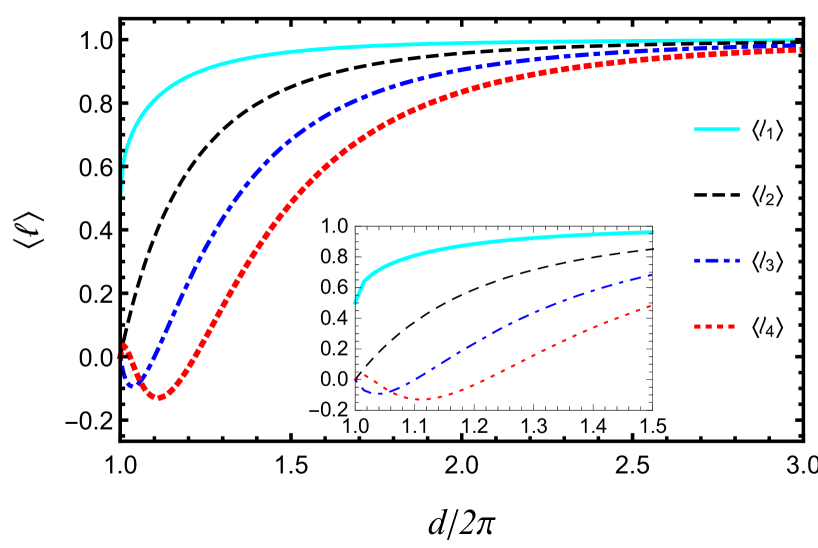
We do not see a general reason why all loops with charge two and higher should vanish at $T_{d}$, Eq. (24), but it obviously follows from the simple form of the eigenvalue density at the transition.

Away from the transition, plots of the charged loops are shown in Fig. 1, plotted versus $d/(2\pi)$. Loops with charge two or greater vanish at the transition, where $d/(2\pi)=1$, but they also begin to oscillate in sign. Again, this is presumably a detailed feature of the model.

In Fig. 2, we show a plot of the value of the first Polyakov loop, $\ell_{1}(T)$, versus results from the lattice. If we require that the transition take place at $T_{d}$, then we must fix $d(T)=2\pi T/T_{d}$, as the transition occurs when $d(T)=2\pi$.

Figure 2: Plot of the Polyakov loop using the solution $d(T)=2\pi T/T_{d}$, versus that for $N_{c}=5$.

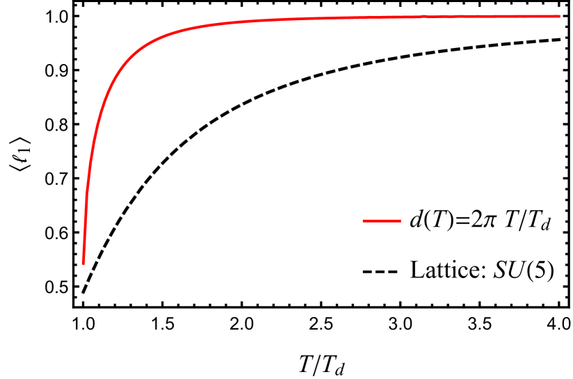
Results for the renormalized Polyakov loop are available for $N_{c}=3$ [50] and higher $N_{c}$ [53]. The results are similar, if not identical. For $N_{c}=3$, the value of the renormalized loop is smaller at $T_{d}$, $\ell_{1}(T_{d})\approx 0.4$. For $N_{c}=5$, $\ell_{1}(T_{d})\approx 0.5$.

Figure 3: Plot of the interaction measure, divided by the number of gluons, $N_{c}^{2}-1$, using the solution $d(T)=2\pi T/T_{d}$, versus that for $N_{c}=3$.

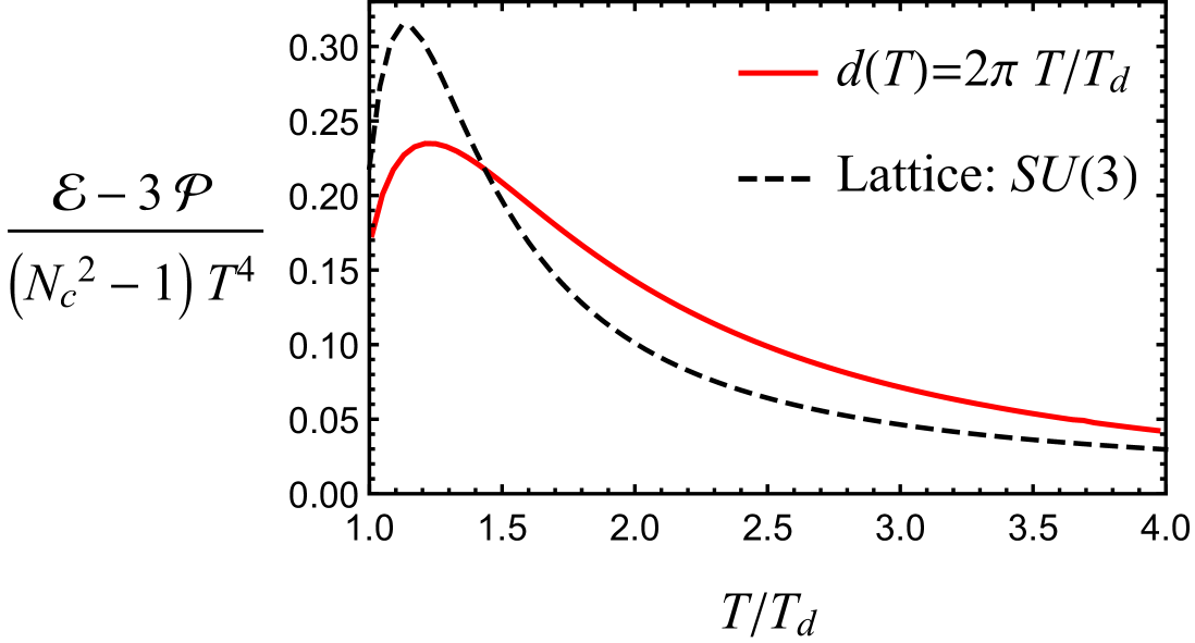
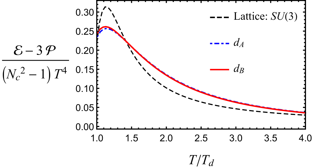
The potential is proportional to the pressure, so one can also immediately compute the entropy density, $s(T)=\partial\mathscr{P}(T)/\partial T$, and from that, the energy density, $\mathscr{E}(T)=Ts(T)-\mathscr{P}(T)$. The deviation from conformality is most easily measured through the “interaction measure”, which is

$$\frac{\mathscr{E}-3\mathscr{P}}{T^{4}}=T\frac{\partial}{\partial T}\left(\frac{\mathscr{P}}{T^{4}}\right)\;.$$ (26)

This is plotted in Fig. 3. The pressure from the matrix model is compared to the lattice results for $N_{c}=3$ [54], as that is the most accurate. From Ref. [54], for three colors the pressure can be fit by the function

$$\mathscr{P}_{\mathrm{lat}}(T)=8\,T^{4}\;\frac{p_{1}+p_{2}\ln(t)+p_{3}\ln^{2}(t)}{8(1+p_{4}\ln(t)+p_{5}\ln^{2}(t))}\;,\;t=\frac{T}{T_{d}}\;,$$ (27)

where $p_{1}=0.0045$, $p_{2}=1.76$, $p_{3}=10.6$, $p_{4}=2.07$, and $p_{5}=5.8$. The overall factor of $8$ on the right-hand side is for the number of gluons. We comment that there are results for the pressure from the lattice for higher $N_{c}$, but the results do not differ significantly from $N_{c}=3$ [55], at least to the accuracy at which we work. We note that very recent work [56] computes thermodynamic quantities across the $SU(3)$ deconfinement transition and presents an improved equation of state, with a similar fit function for the pressure in Eq. (27). We mention that in the analysis for three colors, the pressure was fit to rather good accuracy but at the expense of adding further terms to the pressure [29, 30]. In any case, while the fit to the pressure is approximate, as is obvious from Fig. 2, there is a sharp discrepancy between the Polyakov loop in the matrix model versus the renormalized Polyakov loop from the lattice for $N_{c}=5$. In particular, the Polyakov loop on the lattice approaches unity much slower than in the matrix model. This is not an artifact of large $N_{c}$, and is present in the solution of the matrix model for three colors [29, 30]. This is a serious deficiency of the matrix model, for which we do not have an explanation.

Figure 4: Results for the Polyakov loop with the ansatz of Eq. (28) versus the lattice for $N_{c}=5$.

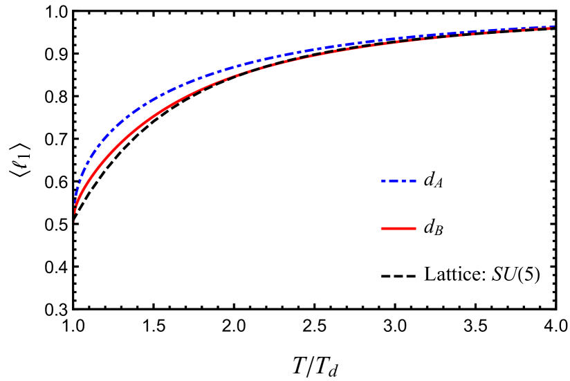
Since we can compute using the matrix model, however, we adopt the following approach. This is admittedly a heuristic approach until said time that a better matrix model can be developed.

We take the solution of the matrix model and adjust $d(T)$ so that the Polyakov loop agrees with the values from the lattice. Accordingly, the terms for the pressure also need to be adapted. We take two ansatzes:

$$d_{A}(T) = 1.08\,t+5.2032\;,$$

$$d_{B}(T) = \frac{0.26}{t^{3}}+1.105\,t+4.9182\;,\;t=\frac{T}{T_{d}}\;.$$ (28)

We take $d_{2}(T)\sim T^{4}$, as for an ideal gas, and define $d_{1}(T)$ from the definition of $d(T)$ in Eq. (17).

The results for the first Polyakov loop are plotted in Fig. 4, where they are compared to the lattice Polyakov loop for $N_{c}=5$. The first form, $d_{A}(T)$, is relatively close to the lattice loop. Given the definition of $d(T)$, $d_{1}(T)\sim d_{2}(T)/d_{A}(T)^{2}$, and so while at large $T$, $d_{1}(T)\sim T^{2}$, as expected from the matrix model, near the transition, the form of $d_{1}(T)$ cannot be motivated except by the fit to the loop. This is even more true for the second form, $d_{B}(T)$, which contains a somewhat arbitrary coefficient $\sim 1/t^{3}$, which is chosen so that there is close agreement with the lattice value of $\ell_{1}$. The results for the interaction measure are shown in Fig. 5. The agreement is satisfactory, although the matrix model does not describe the a sharp peak in the interaction measure at $\sim 1.1T_{d}$.

Figure 5: Results for the interaction measure, divided by the number of degrees of freedom, $N_{c}^{2}-1$, with the ansatz of Eq. (28) versus that, from the lattice, for $N_{c}=3$, Eq. (27).

IV Perturbation theory at nonzero holonomy

It is straightforward to compute at nonzero holonomy by expanding about the background field of Eq. (8). For a detailed discussion, see Ref. [27]. The computation for the gluons is standard so that here we simply establish notation.

We compute at nonzero temperature in Euclidean spacetime, where

$$\int\frac{d^{4}K}{(2\pi)^{4}}=T\sum_{n=-\infty}^{+\infty}\frac{d^{3}k}{(2\pi)^{3}}\;;\;K_{\mu}=(k_{0},\bm{k})\;;\;k_{0}=2\pi nT\;.$$ (29)

In the background field of Eq. (8), for a gluon the time-like component of the momentum is

$$K_{\mu}^{ab}=(k_{0}^{ab},\bm{k})\;,\;k_{0}^{ab}=k_{0}+Q^{ab}=k_{0}+Q^{a}-Q^{b}=2\pi T(n+q_{a}-q_{b})\;.$$ (30)

The difference $q_{a}-q_{b}$ enters because the adjoint covariant derivative involves a commutator of the background field, $A_{0}^{\mathrm{cl}}$. This only happens for the quantum fluctuations with color components that are off-diagonal. For fluctuations that are color diagonal, the background field is not entered. This is the principal reason why computations at nonzero holonomy are more complicated at finite $N_{c}$ than at infinite $N_{c}$.

In the Landau choice of background field gauge, the gluon propagator is

$$D^{\mu\nu}(K^{ab})=\left(\delta^{\mu\nu}-\frac{K_{\mu}^{ab}K_{\nu}^{ab}}{(K^{ab})^{2}}\right)\frac{1}{(K^{ab})^{2}}\;{\mathcal{P}}^{ab,cd}\;.$$ (31)

This involves the color projection operator, $\mathcal{P}^{ab,cd}$, Eq. (10). The three and four-gluon vertices, and the coupling to Faddeev-Popov ghosts, follow directly by replacing the momentum with color flow momenta.

IV.1 Teen fields

We concentrate on the effective theory for the two-dimensional ghost fields [43], which we denote as 3. This is the Bengali character for three, pronounced teen. We chose this because it is simple to write, and it is the third field after gluons and Faddeev-Popov ghosts. We introduce a unit spatial vector $\hat{l}$, and to respect rotational invariance, integrate over all directions of $\hat{l}$. The longitudinal and transverse coordinates with respect to $\hat{l}$ are

$$x^{i}=(\hat{x},\bm{x}_{\perp})\;\;\;,\;\;\;x_{\parallel}=\bm{x}\cdot\hat{l}\;\;\;,\;\;\;\bm{x}_{\perp}\cdot\hat{l}=0\;.$$ (32)

We then introduce gauge covariant derivatives for the fermionic field, $\phi$:

$$S_{\text{\bngx 3}}=\;\int^{1/T}_{0}d\tau\int\frac{d\Omega_{\hat{l}}}{4\pi}\int^{\infty}_{-\infty}dx_{\parallel}\int_{|x_{\perp}^{2}|>1/T_{d}^{2}}d^{2}x_{\perp}\;\mathcal{L}_{\text{\bngx 3}}\;,$$ (33)

where the Lagrangian associated with the $2$D ghost field, i.e.,“teen” field is given by

$$\mathcal{L}_{\text{\bngx 3}}=\;2\;\tr\left((D_{0}\bar{\phi})(D_{0}\phi)+(D_{\parallel}\bar{\phi})(D_{\parallel}\phi)+(\bm{D}_{\perp}\bar{\phi})\cdot(\bm{D}_{\perp}\phi)\right)\;,$$ (34)

and $\phi$ and $\bar{\phi}$ are taken to lie in the adjoint representation. The integral over transverse momenta is explicitly the cutoff at $T_{d}$, and so is manifestly non-perturbative.

In practice, we do not evaluate the effective Lagrangian of Eq. (33) exactly, but directly in momentum space, putting a cutoff on the transverse directions $=T_{d}$. This violates gauge invariance. We show that at one-loop order, this violation does not appear in the teen contribution to the gluon self-energy, but does in the teen self-energy. However, the teen self-energy does not contribute to either the shear or bulk viscosities at leading order, and so for now, we ignore how to implement the teen fields in a more consistent manner.

Now, the teen propagator is

$$D^{ab,cd}_{\text{\bngx 3}}(K)=\frac{1}{(K^{ab})^{2}}\;\mathcal{P}^{ab,cd}\;.$$ (35)

As for the gluons, the interactions follow directly using color flow momenta. The three-point vertex connecting a teen, an anti-teen, and one gluon is

$$-\frac{\delta S_{\text{\bngx 3}}}{\delta\phi^{fe}(R)\,\delta B_{\mu}^{dc}(Q)\,\delta\bar{\phi}^{ba}(P)}=igf^{ab,cd,ef}\,\left(P_{\mu}^{ab}-R^{ef}_{\mu}\right)\;.$$ (36)

Here, $f^{ab,cd,ef}=i(\delta^{ad}\delta^{cf}\delta^{eb}-\delta^{af}\delta^{cb}\delta^{ed})/\sqrt{2}$ is the structure constant. Now, the four-point vertex connecting two gluons and two teen fields is

$$-\frac{\delta S_{\text{\bngx 3}}}{\delta B_{\mu}^{hg}(S)\,\delta B_{\mu}^{fe}(R)\,\delta\bar{\phi}^{dc}(Q)\delta\phi^{ba}(P)\,}=-g^{2}\sum_{ij}(f^{ab,ef,ij}f^{cd,gh,ji}+f^{ab,gh,ij}f^{cd,ef,ji})\,\delta_{\mu\nu}\;.$$ (37)

IV.2 Teen contribution to gluon self-energy

The two contributions to the gluon self-energy from teen fields are illustrated in Fig. 6. As usual, there is a tadpole term, and a term involving two teen fields.

Figure 6: Teen (3) contribution to the gluon self-energy

From Fig. 6a, the tadpole diagram contributes

$$J_{1}^{\mu\nu} = f^{ab,ef,gh}f^{cd,fe,hg}X_{1}^{\mu\nu}\;,$$

$$X_{1}^{\mu\nu} = -2g^{2}\int_{\text{\bngx 3}}\frac{d^{4}k}{(2\pi)^{4}}\frac{\delta^{\mu\nu}}{(K^{fe})^{2}}\;.$$ (38)

The projection operators $\mathcal{P}^{ab,cd}$ are multiplied with traceless generators $t^{ab}$, so the second term $\sim-\delta^{ab}\delta^{cd}/N_{c}$ drops out, and we can take $\mathcal{P}^{ab,cd}\rightarrow\delta^{ac}\delta^{bd}/N_{c}$.

The momentum integral for the teen field is

$$\int_{\text{\bngx 3}}\frac{d^{4}K}{(2\pi)^{4}}=T\sum_{n=-\infty}^{+\infty}\int_{\text{\bngx 3}}\frac{d^{3}k}{(2\pi)^{3}}\;,\;\int_{\text{\bngx 3}}\frac{d^{3}k}{(2\pi)^{3}}=\int_{-\infty}^{+\infty}\frac{dk_{\parallel}}{2\pi}\int_{|k_{\perp}|<T_{d}}\frac{d^{2}k_{\perp}}{(2\pi)^{2}}\;.$$ (39)

Here $k_{\parallel}=\bm{k}\cdot\hat{l}$, and $\bm{k}_{\perp}=\bm{k}-\hat{l}(\bm{k}\cdot\hat{l})$ for a given $\hat{l}$, with $\hat{l}^{\,2}=1$. The integration over all directions of $\hat{l}$ then restores rotational invariance. To simplify the integral over the teen momenta, we will usually assume that $T\gg T_{d}$. This allows us to separate the sum over $n$, with momenta $\sim 2\pi nT$, and $k_{\parallel}$, from the two-dimensional integral over $k_{\perp}$.

The contribution to the self-energy from the self-energy diagram can be written from Fig. 6b as

$$J_{2}^{\mu\nu} = f^{ab,ef,gh}f^{cd,fe,hg}\,X_{2}^{\mu\nu}\;,$$

$$X_{2}^{\mu\nu} = g^{2}\int_{\text{\bngx 3}}\frac{d^{4}K}{(2\pi)^{4}}\frac{(2K^{fe}-P^{ab})^{\mu}(2K^{fe}-P^{ab})^{\nu}}{(K^{fe})^{2}(P^{ab}-K^{fe})^{2}}\;.$$ (40)

The contribution to the gluon self-energy from the two diagrams in the becomes

$$X^{\mu\nu} = X_{1}^{\mu\nu}+X_{2}^{\mu\nu}$$ (41)

$$= -g^{2}\int_{\text{\bngx 3}}\frac{d^{4}K}{(2\pi)^{4}}\bigg{\{}\frac{2\delta^{\mu\nu}}{(K^{fe})^{2}}-\frac{4(K^{fe})^{\mu}(K^{fe})^{\nu}}{(K^{fe})^{2}(P^{ab}-K^{fe})^{2}}\bigg{\}}\;.$$

Here, we neglected the external momentum in the numerator, as the calculation is performed using the HTL approximation in the following. We start with the spatial component of $X_{2}^{\mu\nu}$

$$X_{2}^{ij}(P^{12},Q_{1},Q_{2})=\frac{1}{2}\;g^{2}\int_{\text{\bngx 3}}\frac{d^{3}k}{(2\pi)^{3}}\frac{4k^{i}k^{j}}{4E_{k}E_{p-k}}\left[(\mathcal{I}_{1}+\mathcal{I}_{2}+\mathcal{I}_{3}+\mathcal{I}_{4})+(Q_{1}\leftrightarrow Q_{2})\right]\;.$$ (42)

Here, $E_{k}=|\bm{k}|$, and $E_{p-k}=|\bm{p}-\bm{k}|$. We have symmetrized with respect to $Q_{1}$ and $Q_{2}$, which accounts for the overall factor of $1/2$. In detail,

$$\mathcal{I}_{1} =\frac{-1}{ip^{12}_{0}-E_{k}-E_{p-k}}\Bigl{(}1+n(E_{k}-iQ_{1})+n(E_{p-k}-iQ_{2})\Bigr{)}\;,$$ (43)

$$\mathcal{I}_{2} =\frac{1}{ip^{12}_{0}-E_{k}+E_{p-k}}\Bigl{(}n(E_{k}-iQ_{1})-n(E_{p-k}+iQ_{2})\Bigr{)}\;,$$ (44)

$$\mathcal{I}_{3} =\frac{-1}{ip^{12}_{0}+E_{k}-E_{p-k}}\Bigl{(}n(E_{k}+iQ_{1})-n(E_{p-k}-iQ_{2})\Bigr{)}\;,$$ (45)

$$\mathcal{I}_{4} =\frac{1}{ip^{12}_{0}+E_{k}+E_{p-k}}\Bigl{(}1+n(E_{k}+iQ_{1})+n(E_{p-k}+iQ_{2})\Bigr{)}\;.$$ (46)

To simplify things we write $Q_{1}=Q^{f}-Q^{e}$ and $Q_{2}=Q^{a}-Q^{b}+Q^{f}-Q^{e}$, with $p_{0}^{12}=p_{0}-Q_{1}+Q_{2}$.

The terms that do not involve Landau-damping, and so are due to quasi-particle (QP), can be written as

$$X_{2,\mathrm{QP}}^{ij}(P^{12},Q_{1},Q_{2})=\frac{1}{2}g^{2}\int_{\text{\bngx 3}}\frac{d^{3}k}{(2\pi)^{3}}\frac{{4}k^{i}k^{j}}{4E_{k}E_{p-k}}\left[(\mathcal{I}_{1}+\mathcal{I}_{4})+(Q_{1}\leftrightarrow Q_{2})\right]$$ (47)

$$= g^{2}\int_{\text{\bngx 3}}\frac{d^{3}k}{(2\pi)^{3}}\frac{2\delta^{ij}}{4E_{k}}\frac{\bm{v}_{k}^{\,2}}{3}\bigg{[}n(E_{k}-iQ_{1})+n(E_{k}+iQ_{1})+n(E_{k}-iQ_{2})+n(E_{k}+iQ_{2})\bigg{]}\;,$$

where $\bm{v}_{k}=\bm{k}/E_{k}$. Now, the terms involving Landau damping (LD) are

$$X_{2,\mathrm{LD}}^{ij}(P^{12},Q_{1},Q_{2})={\frac{1}{2}}g^{2}\int_{\text{\bngx 3}}\frac{d^{3}k}{(2\pi)^{3}}\frac{{4}k^{i}k^{j}}{4E_{k}E_{p-k}}\left[(\mathcal{I}_{2}+\mathcal{I}_{3})+(Q_{1}\leftrightarrow Q_{2})\right]$$ (48)

$$= \frac{1}{2}g^{2}\int_{\text{\bngx 3}}\frac{d^{3}k}{(2\pi)^{3}}v^{i}_{k}v^{j}_{k}\bigg{[}\frac{{2}}{ip_{0}^{12}+\bm{p}\cdot\hat{l}}\big{\{}n(E_{k}-iQ_{1})-n(E_{k}+iQ_{1})+n(E_{k}-iQ_{2})-n(E_{k}+iQ_{2})\big{\}}$$

$$- \frac{\bm{p}\cdot\hat{l}}{ip_{0}^{12}+\bm{p}\cdot\hat{l}}\,\frac{\partial}{\partial E_{k}}\big{\{}n(E_{k}-iQ_{1})+n(E_{k}+iQ_{1})+n(E_{k}-iQ_{2})+n(E_{k}+iQ_{2})\big{\}}\bigg{]}\;.$$

The second line of Eq. (48) can be simplified as

$$- \frac{g^{2}}{2}\int_{\text{\bngx 3}}\frac{d^{3}k}{(2\pi)^{3}}\bigg{[}v^{i}_{k}v^{j}_{k}\frac{-ip_{0}^{12}}{ip_{0}^{12}+\bm{p}\cdot\hat{l}}\,\big{\{}n^{\prime}(E_{k}-iQ_{1})+n^{\prime}(E_{k}+iQ_{1})+n^{\prime}(E_{k}-iQ_{2})+n^{\prime}(E_{k}+iQ_{2})\big{\}}$$ (49)

$$\hskip 56.9055pt+\ v^{i}_{k}v^{j}_{k}\,\big{\{}n^{\prime}(E_{k}-iQ_{1})+n^{\prime}(E_{k}+iQ_{1})+n^{\prime}(E_{k}-iQ_{2})+n^{\prime}(E_{k}+iQ_{2})\big{\}}\bigg{]}$$

$$= -\frac{g^{2}}{2}\int_{\text{\bngx 3}}\frac{d^{3}k}{(2\pi)^{3}}\bigg{[}v^{i}_{k}v^{j}_{k}\frac{-ip_{0}^{12}}{ip_{0}^{12}+\bm{p}\cdot\hat{l}}\,\big{\{}n^{\prime}(E_{k}-iQ_{1})+n^{\prime}(E_{k}+iQ_{1})+n^{\prime}(E_{k}-iQ_{2})+n^{\prime}(E_{k}+iQ_{2})\big{\}}$$

$$\hskip 28.45274pt-\delta^{ij}\bigg{(}\frac{1}{E_{k}}-\frac{v_{k}^{2}}{3E_{k}}\bigg{)}\big{\{}n(E_{k}-iQ_{1})+n(E_{k}+iQ_{1})+n(E_{k}-iQ_{2})+n(E_{k}+iQ_{2})\big{\}}\bigg{]}\;,$$

where $n^{\prime}(E-iQ_{1})=\partial n(E-iQ_{1})/\partial E$, etc.

Now, the spatial components of the tadpole term are

$$X_{1}^{ij} =-g^{2}\int\frac{d^{4}K}{(2\pi)^{4}}\delta^{ij}\bigg{[}\frac{1}{K_{1}^{2}}+\frac{1}{K_{2}^{2}}\bigg{]}$$

$$\hskip-11.38092pt=-g^{2}\int\frac{d^{3}k}{(2\pi)^{3}}\delta^{ij}\frac{1}{2E_{k}}\bigg{[}n(E_{k}-iQ_{1})+n(E_{k}+iQ_{1})+n(E_{k}-iQ_{2})+n(E_{k}+iQ_{2})\bigg{]}.$$ (50)

If we add Eqs. (47), (49), and (50), the terms $\sim\delta^{ij}$ vanish.

Collecting the non-vanishing terms, the spatial components of $X^{\mu\nu}$ become

$$X^{ij} =g^{2}\int_{0}^{T_{d}}\frac{k_{\perp}\,dk_{\perp}}{2\pi}\int_{0}^{\infty}\frac{2dk_{\parallel}}{2\pi}\int\frac{d\Omega_{\hat{l}}}{4\pi}\,\frac{\hat{k}^{i}\hat{k}^{j}}{ip_{0}^{12}+\bm{p}\cdot\hat{l}}$$

$$\times\bigg{[}\big{\{}n(E_{k}-iQ_{1})-n(E_{k}+iQ_{1})+n(E_{k}-iQ_{2})-n(E_{k}+iQ_{2})\big{\}}$$

$$\hskip 14.22636pt+ip^{12}_{0}\frac{1}{2}\bigg{\{}n^{\prime}(E_{k}-iQ_{1})+n^{\prime}(E_{k}+iQ_{1})+n^{\prime}(E_{k}-iQ_{2})+n^{\prime}(E_{k}+iQ_{2})\bigg{\}}\bigg{]}\;.$$ (51)

Now, the temporal component of $X^{\mu\nu}$ is

$$X^{00} = -g^{2}\int\frac{d^{4}K}{(2\pi)^{4}}\bigg{[}\frac{1}{K_{1}^{2}}+\frac{1}{K_{2}^{2}}\bigg{]}+\frac{1}{2}g^{2}\int\frac{d^{4}K}{(2\pi)^{4}}\bigg{[}\frac{4(k_{1}^{0})^{2}}{K_{1}^{2}(P^{12}-K_{1})^{2}}+\frac{4(k_{2}^{0})^{2}}{K_{2}^{2}(P^{12}-K_{2})^{2}}\bigg{]}$$ (52)

$$= g^{2}\int\frac{d^{4}K}{(2\pi)^{4}}\bigg{[}\frac{1}{K_{1}^{2}}+\frac{1}{K_{2}^{2}}\bigg{]}-\frac{1}{2}g^{2}\int\frac{d^{4}K}{(2\pi)^{4}}\bigg{[}\frac{4({\bm{k}_{1}})^{2}}{K_{1}^{2}(P^{12}-K_{1})^{2}}+\frac{4({\bm{k}_{2}})^{2}}{K_{2}^{2}(P^{12}-K_{2})^{2}}\bigg{]}\;.$$

Collecting the temporal and spatial components, the total $X^{\mu\nu}$ defined in Eq. (42) becomes

$$X^{\mu\nu} = \frac{g^{2}}{2}\int_{0}^{T_{d}}\frac{k_{\perp}\,dk_{\perp}}{2\pi^{2}}\int_{0}^{\infty}2dk_{\parallel}\int\frac{d\Omega_{\hat{l}}}{4\pi}\,$$ (53)

$$\times \bigg{[}\frac{\bar{K}^{\mu}\bar{K}^{\nu}}{ip_{0}^{12}+\bm{p}\cdot\hat{l}}\big{\{}n(E_{k_{\parallel}}-iQ_{1})-n(E_{k_{\parallel}}+iQ_{1})+n(E_{k_{\parallel}}-iQ_{2})-n(E_{k_{\parallel}}+iQ_{2})\big{\}}$$

$$+ \frac{1}{2}\bigg{(}u^{\mu}u^{\nu}+\frac{ip_{0}^{12}\bar{K}^{\mu}\bar{K}^{\nu}}{ip_{0}^{12}+\bm{p}\cdot\hat{l}}\bigg{)}\big{\{}n^{\prime}(E_{k_{\parallel}}-iQ_{1})+n^{\prime}(E_{k_{\parallel}}+iQ_{1})+n^{\prime}(E_{k_{\parallel}}-iQ_{2})+n^{\prime}(E_{k_{\parallel}}+iQ_{2})\big{\}}\bigg{]}$$

$$= \frac{g^{2}}{2\pi^{2}}\frac{T_{d}^{2}}{2}\bigg{[}-2\pi i\big{(}B_{1}(q_{1})+B_{1}(q_{2})\big{)}T\int\frac{d\Omega_{\hat{l}}}{4\pi}\frac{\bar{K}^{\mu}\bar{K}^{\nu}}{\bar{K}\cdot P^{12}}\bigg{]}+\frac{g^{2}}{2\pi^{2}}\frac{T_{d}^{2}}{2}\bigg{[}u^{\mu}u^{\nu}+ip_{0}^{12}\int\frac{d\Omega_{\hat{l}}}{4\pi}\frac{\bar{K}^{\mu}\bar{K}^{\nu}}{\bar{K}\cdot P^{12}}\bigg{]}$$

$$= \frac{g^{2}}{2\pi^{2}}\frac{T\,T_{d}^{2}}{2}\bigg{[}-2\pi i\big{(}B_{1}(q_{1})+B_{1}(q_{2})\big{)}\bigg{]}\delta\Gamma^{\mu\nu}(P^{12})-\frac{g^{2}}{2\pi^{2}}\frac{T_{d}^{2}}{2}\delta\Pi^{\mu\nu}(P^{12})\;.$$

This involves the functions $\delta\Gamma$ and $\delta\Pi$. $\delta\Pi$ is the usual hard thermal loop function,

$$\delta\Pi^{\mu\nu}(P)=-u^{\mu}u^{\nu}-ip_{0}\int\frac{d\Omega_{\hat{l}}}{4\pi}\frac{\bar{K}^{\mu}\bar{K}^{\nu}}{P\cdot\bar{K}}\;,$$ (54)

where $u^{\mu}=\delta^{\mu 0}$ is a vector in the rest frame of the medium. The other function is

$$\delta\Gamma^{\mu\nu}(P)=-\frac{1}{ip_{0}}\left(\delta\Pi^{\mu\nu}(P)+u^{\mu}u^{\nu}\right)\;.$$ (55)

The null vector $\bar{K}^{\mu}\equiv(i,\hat{l})$, and $B_{1}$ is the first Bernoulli polynomial,

$$B_{1}(q)=|q|_{\mathrm{mod}\,1}-\frac{1}{2}\;.$$ (56)

So, the teen contribution to the gluon self-energy becomes

$$\Pi_{\text{\bngx 3}}^{\mu\nu;ab,cd}(P^{ab}) = J_{1}^{\mu\nu}(P^{ab})+J_{2}^{\mu\nu}(P^{ab})$$ (57)

$$\stackrel{{\scriptstyle\text{HTL}}}{{\approx}} f^{ab,ef,gh}f^{cd,fe,hg}X^{\mu\nu}(P^{ab},Q^{fe},Q^{hg})$$

$$= \delta^{ad,bc}X^{\mu\nu}(P^{ab},Q^{ae},Q^{eb})-\delta^{ab,cd}X^{\mu\nu}(P^{ab},Q^{ca},Q^{ac})\;.$$

For the gluon self-energy, the largest terms are $\sim g^{2}T^{3}$ times $\delta\Gamma$, and $\sim g^{2}T^{2}$ times $\delta\Pi$. For soft momenta $P_{\mu}\sim gT$, the term $\sim g^{2}T^{2}$ is as large as the term at the tree level. Remember that after analytic continuation, this holds as well for the time-like component, $p_{0}^{12}=-i\omega+\epsilon$, with $|\omega|\sim gT$.

For the teen loop in the gluon self-energy, we keep the largest terms, which are $\sim TT_{d}^{2}$ times $\delta\Gamma$, and $\sim T_{d}^{2}$ times $\delta\Pi$. We show shortly when both the gluon and teen contributions are included, that the terms $\sim\delta\Gamma$ cancel [27, 43], as a consequence of the equations of motion. The term $\sim\delta\Pi$ contributes to the gluon self-energy. In keeping the largest terms, we write $\stackrel{{\scriptstyle\text{HTL}}}{{\approx}}$ in Eq. (57) to represent that only the largest terms for soft momenta have been kept.

The contribution to the gluon self-energy from a gluon loop at non-zero holonomy is given in Ref. [27]. The total is

$$\Pi^{\mu\nu;ab,cd}_{\mathrm{total}}(P^{ab}) = \Pi_{\mathrm{gl}}^{\mu\nu;ab,cd}(P^{ab})+\Pi_{\text{\bngx 3}}^{\mu\nu;ab,cd}(P^{ab})$$ (58)

$$= -\mathcal{K}^{ab,cd}\delta\Gamma^{\mu\nu}(P^{ab})-(m^{2})^{ab,cd}\delta\Pi^{\mu\nu}(P^{ab})\;.$$

Now, $\mathcal{K}^{ab,cd}$ in Eq. (58) is

$$\mathcal{K}^{ab,cd} = \frac{2\pi ig^{2}}{3}\,\delta^{ad}\delta^{bc}\bigg{[}\sum_{e=1}^{N_{c}}\bigg{(}\mathcal{A}_{0}(Q^{ae})+\mathcal{A}_{0}(Q^{eb})\bigg{)}T^{3}$$ (59)

$$+\,3\sum_{e=1}^{N_{c}}\frac{1}{8\pi^{3}}\left\{\big{(}B_{1}(q_{a}-q_{e})+B_{1}(q_{e}-q_{b})\big{)}\right\}T_{d}^{2}T\bigg{]}\;,$$

where

$$\mathcal{A}_{0}(Q)=\frac{3}{2\pi iT^{3}}\int\frac{d^{3}k}{(2\pi)^{3}}\left(n(E_{k}-iQ)-n(E_{k}+iQ)\right)\;.$$ (60)

It is direct to show that Eq. (59) vanishes by the equations of motion [43]. Physically, the sum of the currents induced by the gluon and teen field cancel [43]. This is an essential check on the consistency of the model.

The second term in Eq. (58) involves the usual hard thermal loop in the gluon self-energy, $\delta\Pi(P)$, times the Debye mass squared [27, 43]. The latter includes contributions from the gluons and teen fields,

$$(m^{2})^{ab,cd}=(m^{2}_{\mathrm{gl}})^{ab,cd}+\frac{g^{2}T_{d}^{2}}{4\pi^{2}}\mathcal{P}^{ab,cd}\;,$$ (61)

where

$$(m^{2}_{\mathrm{gl}})^{ab,cd}=\frac{g^{2}T^{2}}{6}\left(\delta^{ad}\delta^{bc}\sum_{f=1}^{N_{c}}\left\{\mathcal{A}(Q^{af}+\mathcal{A}(Q^{fb})\right\}-2\delta^{ab}\delta^{cd}\mathcal{A}(Q^{ac})\right)\;,$$ (62)

with

$$\mathcal{A}(Q)=\frac{12}{T^{2}}\int\frac{d^{3}k}{(2\pi)^{3}}\frac{1}{2E_{k}}\left(n(E_{k}-iQ)+n(E_{k}+iQ)\right)\;.$$ (63)

IV.3 Teen self-energy

The diagrams which contribute to the teen self-energy are those of Fig. 7. There is a tadpole diagram, plus a diagram with a virtual gluon teen pair.

Figure 7: Teen self-energy diagrams

As for the usual scalar self-energy, the teen self-energy is gauge-dependent. Thus we content ourselves with power counting. The tadpole diagram, Fig. 7a, only involves a virtual gluon, and so is proportional to $\sim g^{2}T^{2}$. The diagram with a gluon-teen pair involves a virtual teen field, Fig. 7b involves an integral over a teen field, and so is automatically $\sim g^{2}T_{d}^{2}$. We shall see, however, that the teen self-energy does not enter into the computation of the shear and bulk viscosities at leading logarithmic order. As we demonstrate in the following, this is not obvious, and due to which the diagrams in detail contribute at leading logarithmic order.

V Shear viscosity

V.1 Scattering amplitude

We follow the perturbative computation of the shear viscosity following Arnold, Moore, and Yaffe [44, 45, 57, 58, 59, 60, 61, 62, 63], modified to the case of nonzero holonomy [25, 28].

Figure 8: Kinematics of 2-2 scattering, from Ref. [26]

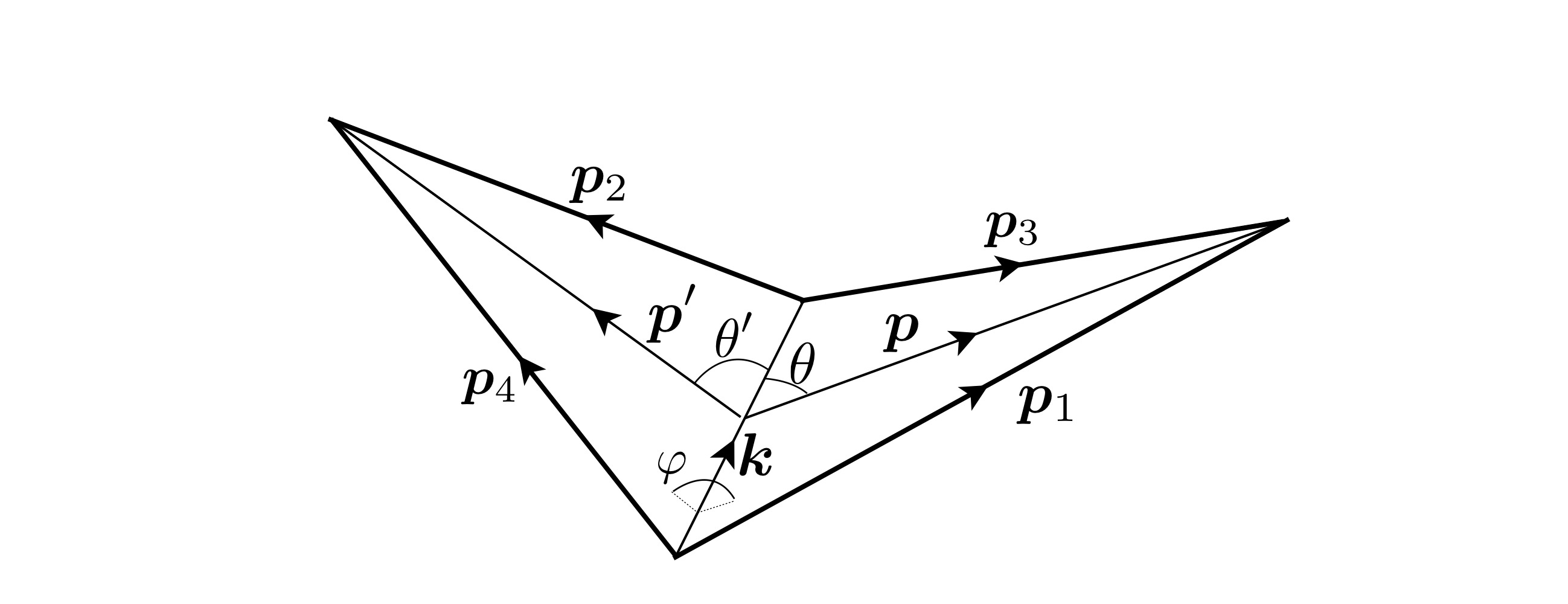
At leading order, what contributes is the scattering of two to two scattering: two incident particles, with momenta $P_{1}$ and $P_{2}$, go into fields with momenta $P_{3}$ and $P_{4}$. The particles can be either gluon or teen fields. For $2\rightarrow 2$ scattering, the Mandelstam variables are

$$s=(P_{1}+P_{2})^{2}\;,\;t=(P_{1}-P_{3})^{2}\;,\;u=(P_{1}-P_{4})^{2}\;.$$ (64)

It is convenient to parametrize these momenta as

$$P_{1}=P+\frac{K}{2}\;,\;P_{2}=P^{\prime}-\frac{K}{2}\;,P_{3}=P-\frac{K}{2}\;,P_{4}=P^{\prime}+\frac{K}{2}\;.$$ (65)

The dominant contribution to the shear and bulk viscosities is forward scattering. The momenta $P_{1}$ and $P_{2}$, and $P_{3}$ and $P_{4}$, are hard, with the components of the momenta on the order of the temperature, $T$. The exchanged momentum in the $t$-channel, $K$, is soft, on the order of $gT$. We introduce the angles $\theta$ and $\theta^{\prime}$

$$\cos\theta=\hat{\bm{k}}\cdot\hat{\bm{p}}\;,\hskip 56.9055pt\cos\theta^{\prime}=\hat{\bm{k}}\cdot\hat{\bm{p}}^{\prime}\;,$$ (66)

as illustrated in Fig. 8. We define the unit vector $\hat{\bm{k}}=\bm{k}/k$, where $k=|\bm{k}|$, and $\phi$ as the angle between two planes spanned by vectors $(\bm{p}_{1},\bm{p}_{3})$ and $(\bm{p}_{2},\bm{p}_{4})$.

For forward scattering,

$$\cos\theta\simeq x\equiv\frac{k_{0}}{k}\;,$$ (67)

and $\theta\approx\theta^{\prime}$, with

$$\cos\phi\simeq\frac{\hat{\bm{p}}\cdot{\hat{\bm{p}}^{\prime}}-x^{2}}{1-x^{2}}\;.$$ (68)

The Mandelstam variables become

$$s \simeq 2pp^{\prime}(1-x^{2})(1-\cos\phi)\;,$$

$$u \simeq -2pp^{\prime}(1-x^{2})(1-\cos\phi)\;,$$

$$t \simeq -k^{2}(1-x^{2})\;.$$ (69)

We only consider the diagrams that contribute to the leading logarithmic order for the shear and bulk viscosity. These are the $t$- and $u$-channels, where a soft field is exchanged in the $t$-channel; the $u$-channel is related to the $t$-channel by exchanging $P_{3}\leftrightarrow P_{4}$. Thus, we neglect diagrams where soft fields are exchanged in other channels, and diagrams with four-point interactions, which include those between four gluons, or two gluons and two teens.

The diagrams that contribute to leading logarithmic orders are of two types. There are those involving the exchange of a soft gluon, illustrated in Figs. 9a-c, and those involving the exchange of a soft teen field, illustrated in Figs. 10a,b.

V.1.1 Exchange of a soft, virtual gluon

Figure 9: The diagrams involving the exchange of a virtual soft gluon: gluon-gluon scattering (a), gluon-teen scattering (b), and teen-teen scattering (c).

The amplitude for two gluons scattering into two gluons, Fig. 9a, is

$$\mathcal{M}_{{\mathrm{gg}}\rightarrow{\mathrm{gg}}}=\epsilon_{1}^{\mu_{1}}(P_{1}^{a_{1}b_{1}})\,\epsilon_{3}^{*\mu_{3}}(P_{3}^{a_{3}b_{3}}) J_{{\mathrm{g}},\mu_{1}\mu_{3}}^{\mu,ab}(P_{1}^{a_{1}b_{1}},P_{3}^{a_{3}b_{3}})\,D_{\mu\nu}^{ba,dc}(K^{ba})\,$$ (70)

$$\times\ J_{\mathrm{g},\mu_{2}\mu_{4}}^{\nu,cd}(P_{2}^{a_{2}b_{2}},P_{4}^{a_{4}b_{4}})\;\epsilon_{2}^{\mu_{2}}(P_{2}^{a_{2}b_{2}})\,\epsilon_{4}^{*\mu_{4}}(P_{4}^{a_{4}b_{4}})\;.$$

Here $P_{i}^{\mu,a_{i},b_{i}}$ are the momenta for particles $i=1,\ldots,4$. The polarization tensor are $\epsilon_{1,2}^{\mu}$ for incoming particles, and $\epsilon_{3,4}^{*\mu}$ for outgoing fields. They satisfy

$$\epsilon_{i}^{\mu}(P_{i}^{a_{i}b_{i}})\,P_{\mu,i}^{a_{i}b_{i}}=\epsilon_{i}^{*\mu}(P_{i}^{a_{i}b_{i}})\,P_{\mu,i}^{a_{i}b_{i}}=0\;.$$ (71)

In these expressions, we keep the color indices because especially Eq. (70) makes it clear how the color flow works. They really are not necessary in Eq. (71), though, since the on-shell condition only applies after analytic continuation to Minkowski momenta, $p_{0}^{ab}\rightarrow-i\omega$.

In Eq. (70), $D_{\mu\nu}^{ba,dc}(K^{ba})$ is the gluon propagator of Eq. (31). Now, the color current for a gluon is

$$J_{{\mathrm{g}},\mu_{1}\mu_{3}}^{\mu,ab}(P_{1}^{a_{1}b_{1}},P_{3}^{a_{3}b_{3}})=2igP^{\mu,ab}\;\delta^{\mu_{1}\mu_{3}}\;t^{ab}_{a_{1}b_{1},a_{3}b_{3}}\;.$$ (72)

We suppress the two spin indices for a spin-one gluon since that is just an overall degeneracy. The generator in the adjoint representation is

$$t^{ab}_{cd,ef}=i\,f^{(ab,cd,ef)}=\frac{i}{\sqrt{2}}\left(\delta^{ad}\delta^{cf}\delta^{be}-\delta^{af}\delta^{bc}\delta^{de}\right)\;,$$ (73)

as defined in Eq. (24) of Ref. [27]. In the matrix element, we only consider forward scattering, where $P^{a_{1}b_{1}}_{1}\simeq P^{a_{3}b_{3}}_{3}\simeq P^{ab}$. All of the external gluon momenta are hard, $P^{a_{i}b_{i}}\sim T$.

The scattering for a teen plus gluon scattering into the same is shown in Fig. 9b. The teen field has spin-zero, and so no spin degeneracy. The scattering amplitude in the $t$-channel is

$$\mathcal{M}_{\text{\bngx 3}{\mathrm{g}}\rightarrow\text{\bngx 3}{\mathrm{g}}}=J_{\text{\bngx 3}}^{\mu,ab}(P_{1}^{a_{1}b_{1}},P_{3}^{a_{3}b_{3}})\,D_{\mu\nu}^{ba,dc}(K^{ba})\,J_{{\mathrm{g}},\mu_{2}\mu_{4}}^{\nu,cd}(P_{2}^{a_{2}b_{2}},P_{4}^{a_{4}b_{4}})\,\epsilon^{\mu_{2}}(P^{a_{2}b_{2}}_{2})\,\epsilon^{*\mu_{4}}(P^{a_{4}b_{4}}_{4})\;,$$ (74)

where $J_{\text{\bngx 3}}^{\mu;ab}$ is the color current associated with teen (3)-gluon vertex,

$$J_{\text{\bngx 3}}^{\mu,ab}(P_{1}^{a_{1}b_{1}},P_{3}^{a_{3}b_{3}})=2igP^{\mu,ab}\,t^{ab}_{a_{1}b_{1},a_{3}b_{3}}\;.$$ (75)

The color structure is identical to that of the gluon, Eq. (72), as both lie in the adjoint representation. Since the teen particle is a scalar, though, there is no factor of $\delta^{\mu_{1}\mu_{3}}$, as in the gluon current of Eq. (72).

There is another implicit difference: the perpendicular component of the teen momenta $P^{a_{1}b_{1}}_{1}$ and $P^{a_{2}b_{2}}_{2}$ are of the order of $T_{d}$. Thus, when a soft gluon is exchanged with $K\sim gT$, $k_{\perp}$ is also restricted to be $\sim T_{d}$.

The scattering amplitude for teen plus teen scattering into the same, Fig. 9c, is

$$\mathcal{M}_{\text{\bngx 3}\text{\bngx 3}\rightarrow\text{\bngx 3}\text{\bngx 3}}=J_{\text{\bngx 3}}^{\mu;ab}(P_{1}^{a_{1}b_{1}},P_{3}^{a_{3}b_{3}})\,D_{\mu\nu}^{ba,dc}(K^{ba})\,J_{\text{\bngx 3}}^{\nu;cd}(P_{2}^{a_{2}b_{2}},P_{4}^{a_{4}b_{4}})\;.$$ (76)

V.1.2 Exchange of a soft teen field

Figure 10: The diagrams involving the exchange of a soft, virtual teen particle: Compton scattering (a) and teen-teen annihilation (b).

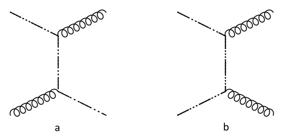
There are two diagrams involving the exchange of a teen particle. One contribution is where a teen plus a gluon scatters into a gluon plus a teen, Fig. 10a. This is analogous to Compton scattering. The amplitude is

$$\mathcal{M}_{\text{\bngx 3}{\mathrm{g}}\rightarrow{\mathrm{g}}\text{\bngx 3}}=\epsilon^{\mu}(P^{a_{1}b_{1}}_{1})\,J_{\text{\bngx 3}}^{\mu,ab}(P^{a_{1}b_{1}}_{1},P^{a_{3}b_{3}}_{3})\,D_{\text{\bngx 3}}^{ba,dc}(K^{ba})\,J_{\text{\bngx 3}}^{\nu,cd}(P^{a_{2}b_{2}}_{2},P^{a_{4}b_{4}}_{4})\,\epsilon^{*\nu}(P^{a_{4}b_{4}}_{4})\;.$$ (77)

Lastly, there is the scattering of two teens into two gluons, illustrated in Fig. 10b. The amplitude is

$$\mathcal{M}_{\text{\bngx 3}\text{\bngx 3}\rightarrow{\mathrm{gg}}}=J_{\text{\bngx 3}}^{\mu,ab}(P^{a_{1}b_{1}}_{1},P^{a_{3}b_{3}}_{3})\,D_{\text{\bngx 3}}^{ba,dc}(K^{ba})\,J_{\text{\bngx 3}}^{\nu,cd}(P^{a_{2}b_{2}}_{2},P^{a_{4}b_{4}}_{4})\epsilon^{*\mu}(P^{a_{3}b_{3}}_{3})\,\epsilon^{*\nu}(P^{a_{4}b_{4}}_{4})\;.$$ (78)

These are identical to the diagrams involving gluon exchange, with the replacement of the gluon by the teen particle.

The matrix elements for the teen particle, however, simplify significantly. Consider the factors of the polarization tensor for the scattering of two gluons into two gluons, Eq. (70). This involves

$$\mathcal{M}_{{\mathrm{gg}}\rightarrow{\mathrm{gg}}}\sim g^{2}\;\left(\epsilon^{\mu_{1}}(P^{a_{1}b_{1}}_{1})\epsilon^{*}_{\mu_{1}}(P^{a_{3}b_{3}}_{3})\right)\;\left(\epsilon^{\mu_{2}}(P^{a_{2}b_{2}}_{2})\epsilon^{*}_{\mu_{2}}(P^{a_{4}b_{4}}_{4})\right)\;\ldots\;,$$ (79)

where for simplicity, we drop the other factors. For all of the other diagrams involving gluon exchange, the polarization tensors are contracted with one another, and so give contributions to the leading order in the coupling constant, $\sim g^{2}$.

In contrast, consider the scattering of a teen plus gluon into a gluon plus teen, Fig. 10a. Including just the factors of the polarization tensor, which is

$$\mathcal{M}_{\text{\bngx 3}{\mathrm{g}}\rightarrow{\mathrm{g}}\text{\bngx 3}}\;\sim\;g^{2}\;\left(\epsilon^{\mu}(P^{a_{1}b_{1}}_{1})P^{ab}_{\mu}\right)\;\left(\epsilon^{*\nu}(P^{a_{4}b_{4}}_{4})P^{ab}_{\nu}\right)\;\sim g^{4}\;.$$ (80)

Each of the polarization vectors dotted into the momentum of that field vanishes, such as $\epsilon^{\mu}_{1}P^{a_{1}b_{1}}_{1\mu}=0$, etc., Eq. (71). Then the momentum that appears in the current, $\sim P^{ab}_{\mu}$, is approximately equal to the external momenta, such as $P^{a_{1}b_{1}}_{1\mu}$, up to soft corrections, $\sim K^{ba}_{\mu}$. These terms are, by assumption, suppressed by $\sim g$. Thus in all, the matrix elements involving the exchange of a teen particle, Fig. 10, are only $\sim g^{4}$, relative to those involving gluon exchange, Fig. 9, which are $\sim g^{2}$.

This cancellation for the scattering of the scalar field is well known. As discussed in Sec. IV.3, this is most fortunate, and these subtleties associated with constructing a complete, and gauge invariant description of the teen fields can thus be overlooked to leading, logarithmic order.

V.2 Collision integrals

To evaluate the transport coefficients, we use kinetic theory. The Boltzmann equation described the evolution of the particle distribution function $f_{ab}({\bf\it r},{\bf\it p},t)$ in phase space. The Boltzmann equation accounts for advection due to motion, external forces, and collisions among particles.

The Boltzmann equation is evaluated using the Chapman-Enskog method. The distribution function $f_{ab}({\bf\it r},{\bf\it p},t)$ is expanded in a series in powers of the Knudsen number $\epsilon$, which quantifies the ratio of the mean free path to the characteristic length scale of the system. This expansion assumes that the system is close to local equilibrium, allowing for the separation of equilibrium and non-equilibrium contributions to the distribution function.

At zeroth order $\epsilon^{0}$, the collisions among particles are neglected, and the equilibrium distribution function $f_{ab}^{0}$ is obtained. Deviations from equilibrium enter at $\epsilon^{1}$. By substituting the zeroth-order solution into the Boltzmann equation and retaining terms linear in $\epsilon$, a linearized Boltzmann equation is obtained. Solving this equation iteratively yields the first-order correction to the distribution function $f^{1}_{ab}$, capturing the effects of collisions on the distribution of particles.

The shear viscosity $\eta$ is then extracted from the correction at first order, $f^{1}_{ab}$. This involves calculating the momentum flux tensor and comparing it to the gradient of the velocity field, quantifying the resistance to shear flow in the plasma.

Finally, the obtained expression for shear viscosity undergoes various consistency checks to ensure its physical validity. These checks may involve verifying that $\eta$ is positive, and exhibits the correct behavior in the limit of a small Knudsen number.

The energy-momentum tensor for the gluon is given by

$$T^{\mu\nu}_{\mathrm{g}}(\bm{r},t)=2\int_{\mathrm{g}}d\Gamma_{ab}\;P^{\mu,ab}P^{\nu,ab}\;f_{{\mathrm{g}},ab}({\bf\it r},\bm{p},t)\;,$$ (81)

where $f_{\mathrm{g},ab}(\bm{r},\bm{p},t)$ is the statistical distribution function for the gluon. In thermal equilibrium, this is the Bose-Einstein distribution function in a background field $Q^{a}-Q^{b}$,

$$f^{0}_{{\mathrm{g}},ab}=f^{0}_{ab}(E_{p})\equiv\frac{1}{\mathrm{e}^{(E_{p}-i(Q^{a}-Q^{b}))/T}-1}\;,$$ (82)

with $E_{p}=\sqrt{\bm{p}^{\,2}}$ the energy. The phase space integral is

$$\int_{\mathrm{g}}d\Gamma_{ab}=\sum_{s}\sum_{a,b=1}^{N_{c}}\;\mathcal{P}^{ab,ba}\;\int\frac{d^{3}p}{(2\pi)^{3}2E_{p}}\;.$$ (83)

This includes a sum over the colors $a,b$, and the helicity $s$. The factor $\mathcal{P}^{ab,ba}$ ensures that the overall number of degrees of freedom is $N_{c}^{2}-1$, as appropriate for $SU(N_{c})$.

The teen field is analogous to a Faddeev-Popov ghost field and is an anti-commuting field in the adjoint representation. An anti-commuting field is normally a fermion. Fermions, however, are anti-periodic in the imaginary time, $\tau$, under the shift $\tau\rightarrow\tau+1/T$. Instead, in thermal equilibrium, the teen field should be periodic in $\tau$, like a gluons. Consequently, for the teen field, we start with the statistical distribution function for a fermion, after shifting $(Q^{a}-Q^{b})$ by $\pi T$:

$$\frac{1}{\mathrm{e}^{(E_{p}-i(Q^{a}-Q^{b}+\pi T))/T}+1}={\color[rgb]{0,0,0}(-)}f^{0}_{ab}(E)\;.$$ (84)

Thus absorption of a teen field from a thermal bath produces a relative minus sign, versus that of a gluon. This shows that the teen field is a ghost. To keep track of the signs, we introduce a sign function, which $=+1$ for gluons, and $=-1$ for teens,

$${\mathcal{S}}_{\mathrm{g}}=+1\;\;;\;\;{\mathcal{S}}_{\text{\bngx 3}}=-1\;.$$ (85)

In equilibrium, we find it useful to take the statistical distribution function for the teen equal to that for the gluon,

$$f^{0}_{\text{\bngx 3},ab}(E_{p})={\color[rgb]{0,0,0}(+)}f_{{\mathrm{g}},ab}^{0}(E_{p})\;.$$ (86)

If we take the distribution functions to be the same, then because there is a $(-)$ sign on the right hand side of Eq. (84), whenever a single factor of a statistical distribution function enters for absorption from the medium, $=f^{0}_{ab}(E)$, we have to multiply that by the sign function: ${\mathcal{S}}_{\text{\bngx 3}}=-1$ for a teen field, and ${\mathcal{S}}_{\mathrm{g}}=+1$ for a gluon.

This is not true for emission into the medium, however. For a fermion with a statistical distribution function $f^{0}_{\mathrm{ferm},ab}(E)$, emission is associated with the factor $1-f^{0}_{\mathrm{ferm},ab}(E)$. In this case, the minus sign reflects the Pauli exclusion principle. For a teen field, then, by Eq. (84) this becomes $1+f^{0}_{\mathrm{g},ab}(E)$. Thus for a teen field, there is no sign function, which arises when it is emitted into the medium. This is why we prefer to keep the signs of the teen and gluon distribution functions the same, Eq. (86), and instead introduce the sign functions ${\mathcal{S}}_{\text{\bngx b}}$, etc., for absorption.

It is useful to compare these signs to the case where gluons scatter off of physical fermions, which we do in Appendix A. Because they are physical, fermions do not have a $(-)$ sign when they are absorbed from the medium, while teen particles, which are ghosts, do.

The teen contribution to the stress-energy tensor is

$$T^{\mu\nu}_{\text{\bngx 3}}={2}\int_{\text{\bngx 3}}d\Gamma_{ab}\;P^{\mu,ab}P^{\nu,ab}\;\,{{\mathcal{S}}_{\text{\bngx 3}}}\;f_{\text{\bngx 3},ab}\;.$$ (87)

This contributes to the pressure with a negative sign, which is what is expected for a ghost field. As explained previously, we need a ghost to decrease the pressure as the temperature is lowered, and the confined phase is approached.

While the gluon and teen distribution functions are equal in equilibrium, they differ away from equilibrium. Thus, there is a Boltzmann equation describing the evolution of each distribution function.

In the absence of collisions, for a system in the background gauge fields $A_{\mu}$ and with total color charge ${\cal Q}$, the gluon statistical distribution function satisfies the Vlasov equation [19, 20, 21],

$$P^{\mu}\left(\frac{\partial}{\partial x_{\mu}}-g\,\tr\left({\cal Q}G_{\mu\nu}\right)\frac{\partial}{\partial p_{\nu}}-ig\left[{\cal Q},\frac{\partial}{\partial{\cal Q}}\right]\right)f(x,p,{\cal Q})=0\;.$$ (88)

In the semi-QGP, however, since $A_{0}^{\rm cl}$ is constant, the field strength vanishes, $G_{\mu\nu}=0$. Further, as shown by Eq. (59), the total color charge vanishes ${\cal Q}=0$. Thus, only the first term on the left hand side of Eq. (88) contributes, and we must consider the effect of collisions in the Boltzmann equation.

For collisions, we include the scattering of $2\rightarrow 2$ particles to lowest order,

$$1_{\text{\bngx b}}\;2_{\text{\bngx d}}\rightarrow 3_{{\text{\bngx b}^{\prime}}}\,\;4_{{\text{\bngx d}^{\prime}}}\;.$$ (89)

The associated momenta are $P^{\mu,a_{1}b_{1}}_{1}$, etc. We introduce the symbols b, d, $\text{\bngx b}^{\prime}$, and $\text{\bngx d}^{\prime}$ to denote that these particles can be either gluon or teen fields. The Boltzmann equation is

$${\mathcal{S}}_{\text{\bngx b}}\;2P^{\mu,a_{1}b_{1}}\partial_{\mu}f_{\text{\bngx b},a_{1}b_{1}}(\bm{x},\bm{p},t)=-{\mathcal{C}}_{\text{\bngx b},a_{1}b_{1}}[f_{\text{\bngx b}}]\;,$$ (90)

where the collisional kernel is

$${\mathcal{C}}_{\text{\bngx b},a_{1}b_{1}}[f_{\text{\bngx b}}] ={\frac{1}{2}}\,{\sum_{\text{\bngx d},\text{\bngx b}^{\prime},\text{\bngx d}^{\prime}}}{\mathcal{S}}_{\text{\bngx b}}\,{\mathcal{S}}_{\text{\bngx d}}\int_{\text{\bngx d}}d\Gamma_{a_{2}b_{2}}\,\int_{\text{\bngx b}^{\prime}}d\Gamma_{a_{3}b_{3}}\,\int_{\text{\bngx d}^{\prime}}d\Gamma_{a_{4}b_{4}}\,(2\pi)^{4}$$

$$\times\delta^{(4)}(P^{a_{1}b_{1}}_{1}+P^{a_{2}b_{2}}_{2}-P^{a_{3}b_{3}}_{3}-P^{a_{4}b_{4}}_{4})\;|\mathcal{M}_{\text{\bngx b}\text{\bngx d}\rightarrow\text{\bngx b}^{\prime}\text{\bngx d}^{\prime}}|^{2}$$

$$\hskip 0.0pt\times\left[f_{\text{\bngx b},a_{1}b_{1}}f_{\text{\bngx d},a_{2}b_{2}}\left(1+f_{\text{\bngx b}^{\prime},a_{3}b_{3}}\right)\left(1+f_{\text{\bngx d}^{\prime},a_{4}b_{4}}\right)\right.$$

$$\left.\hskip 28.45274pt-f_{\text{\bngx b}^{\prime},a_{3}b_{3}}f_{\text{\bngx d}^{\prime},a_{4}b_{4}}\left(1+f_{\text{\bngx b},a_{1}b_{1}}\right)\left(1+f_{\text{\bngx d},a_{2}b_{2}}\right)\right].$$ (91)

The only subtlety is the sign factors. The sign factor ${\mathcal{S}}_{\text{\bngx b}}$ enters on the left hand side of Eq. (90), as that describes the distribution function for the initial particle, $1_{\text{\bngx b}}$.

On the right-hand side, in the collision term of Eq. (91), there are only symmetry factors for particles absorbed from the medium. This is ${\mathcal{S}}_{\text{\bngx b}}\,{\mathcal{S}}_{\text{\bngx d}}$ for the first term, and ${\mathcal{S}}_{\text{\bngx b}^{\prime}}{\mathcal{S}}_{\text{\bngx d}^{\prime}}$ for the second. Since teen number is conserved, however, the sign factors satisfy

$${\mathcal{S}}_{\text{\bngx b}}\;{\mathcal{S}}_{\text{\bngx d}}={\mathcal{S}}_{\text{\bngx b}^{\prime}}\;{\mathcal{S}}_{\text{\bngx d}^{\prime}}\;.$$ (92)

It is easy to convince oneself by working out all of the examples, such as $\text{\bngx 3}{\mathrm{g}}\rightarrow\text{\bngx 3}{\mathrm{g}}$, etc. Because of this, in Eq. (91) we can write the sign factors of both terms as a common prefactor, $={\mathcal{S}}_{\text{\bngx b}}\,{\mathcal{S}}_{\text{\bngx d}}$.

With the Chapman-Enskog method, the time derivative is expanded in the power of $\epsilon$

$$\partial_{t}=\sum_{n=1}^{\infty}\epsilon^{n}\partial_{t}^{(n)}.$$ (93)

We expand the distribution function around the distribution function in thermal equilibrium, $f^{0}_{ab}$,

$$f_{\text{\bngx b},ab}=f^{0}_{ab}+\epsilon f^{1}_{\text{\bngx b},ab}+\epsilon^{2}f^{2}_{\text{\bngx b},ab}+\cdots\;.$$ (94)

Notice that the index b does not enter into the distribution function as lowest order, because in equilibrium the gluon and teen distribution functions are the same as given in Eq. (86). Thus we generally replace $f_{\text{\bngx b},ab}^{0}(E)$ by $f_{ab}^{0}(E)$. We parametrize $f^{n}_{\text{\bngx b},ab}$ as

$$f^{n}_{\text{\bngx b},ab}=\ f^{0}_{ab}(1+f^{0}_{ab})\phi_{\text{\bngx b},ab}^{(n)}\;.$$ (95)

Because we introduced the sign functions above, there is no need to introduce a sign function in the definition of $\phi_{\text{\bngx b},ab}^{(n)}$.

To $\epsilon^{n}$ order, the Boltzmann equation is

$${\mathcal{S}}_{\text{\bngx b}}\,2P^{\mu,{a_{1}b_{1}}}\partial_{\mu}^{(n)}f_{\text{\bngx b},a_{1}b_{1}}=-(\mathcal{L}\phi^{(n)})_{\text{\bngx b},a_{1}b_{1}}+K^{(n)}_{\text{\bngx b},a_{1}b_{1}}\;,\;K^{(n)}_{\text{\bngx b},a_{1}b_{1}}=-{\mathcal{C}}^{(n)}_{\text{\bngx b},a_{1}b_{1}}+(\mathcal{L}\phi^{(n)})_{\text{\bngx b},a_{1}b_{1}}\;.$$ (96)

The linearized operator $\mathcal{L}$ is

$$(\mathcal{L}\phi^{(n)})_{\text{\bngx b},a_{1}b_{1}} =\frac{1}{2}\sum_{\text{\bngx d},\text{\bngx b}^{\prime},\text{\bngx d}^{\prime}}{\mathcal{S}}_{\text{\bngx b}}{\mathcal{S}}_{\text{\bngx d}}\int_{\text{\bngx d}}d\Gamma_{a_{2}b_{2}}\int_{\text{\bngx b}^{\prime}}d\Gamma_{a_{3}b_{3}}\int_{\text{\bngx d}^{\prime}}d\Gamma_{a_{4}b_{4}}$$

$$\times\,(2\pi)^{4}\delta^{(4)}(P^{a_{1}b_{1}}_{1}+P^{a_{2}b_{2}}_{2}-P^{a_{3}b_{3}}_{3}-P^{a_{4}b_{4}}_{4})|\mathcal{M}_{\text{\bngx b}\text{\bngx d}\rightarrow\text{\bngx b}^{\prime}\text{\bngx d}^{\prime}}|^{2}$$

$$\hskip 4.26773pt\times\left[f_{a_{1}b_{1}}^{0}f_{a_{2}b_{2}}^{0}(1+f_{a_{3}b_{3}}^{0})(1+f_{a_{4}b_{4}}^{0})\right]\left(\phi_{\text{\bngx b},a_{1}b_{1}}^{(n)}+\phi_{\text{\bngx d},a_{2}b_{2}}^{(n)}-\phi_{\text{\bngx b}^{\prime},a_{3}b_{3}}^{(n)}-\phi_{\text{\bngx d}^{\prime},a_{4}b_{4}}^{(n)}\right).$$ (97)

The right-hand side includes a sum over both gluons and teens. To order $\epsilon^{n}$,

$$P^{\mu,a_{1}b_{1}}\partial_{\mu}^{(n)}f_{\text{\bngx b},a_{1}b_{1}}=p^{0,a_{1}b_{1}}\sum_{k=1}^{n}\partial_{t}^{(k)}f_{{\text{\bngx b},t},a_{1}b_{1}}^{n-k}+p^{i}\partial_{i}f_{{\text{\bngx b},t},a_{1}b_{1}}^{n-1}\;.$$ (98)

To leading order, the viscosities are computed from

$${\mathcal{S}}_{\text{\bngx b}}\;2P^{\mu,a_{1},b_{1}}\partial_{\mu}^{(1)}f_{\text{\bngx b},a_{1}b_{1}}=-(\mathcal{L}\phi^{(1)})_{\text{\bngx b},a_{1}b_{1}}\;,$$ (99)

with $K^{1}=0$.

We assume that near equilibrium, that the four velocity of the medium is $\beta u^{\mu}$, where $\beta=1/T$ is the temperature, and $u^{\mu}=(1,\bm{u})/\sqrt{1-\bm{u}^{2}}$ the velocity. It suffices to work to linear order in $|\bm{u}|$. Then, except for an overall factor of ${\mathcal{S}}_{\text{\bngx b}}$, the left-hand side of the Boltzmann equation is

$$2P^{\mu,a_{1}b_{1}}\partial_{\mu}^{(1)}f^{0}_{\text{\bngx b},a_{1}b_{1}} =-2P^{\mu,a_{1}b_{1}}f^{0}_{a_{1}b_{1}}(1+f^{0}_{a_{1}b_{1}})(P^{\nu,a_{1}b_{1}}\partial^{(1)}_{\mu}(\beta u_{\nu})-i\partial^{(1)}_{\mu}\nu^{a_{1}b_{1}})$$

$$=-f^{0}_{a_{1}b_{1}}(1+f^{0}_{a_{1}b_{1}})\Bigl{[}2(P^{0,a_{1}b_{1}})^{2}\partial^{(1)}_{t}\beta+2p^{i}P^{0,a_{1}b_{1}}(\partial_{i}\beta+\beta\partial^{(1)}_{t}u_{i})$$

$$\quad+p^{j}p^{i}\beta\sigma_{ij}-\frac{2}{3}p^{2}\beta\partial_{k}u^{k}-2P^{\mu,a_{1}b_{1}}i\partial^{(1)}_{\mu}\nu^{a_{1}b_{1}}\Bigr{]}\;,$$ (100)

where

$$\sigma_{ij}=\partial_{i}u_{j}+\partial_{j}u_{i}-\frac{2}{3}\,\delta^{ij}\,\partial_{k}u_{k}\;,$$ (101)

and $\nu^{ab}=\beta(Q^{a}-Q^{b})=2\pi(q_{a}-q_{b})$.

Using energy-momentum conservation or hydrodynamic equations to leading order,

$$\partial^{(1)}_{t}\beta = \beta v_{s}^{2}\partial_{i}u^{i}\;,$$ (102a)

$$\beta\partial^{(1)}_{t}u_{i} = -\partial_{i}\beta\;,$$ (102b)

where the speed of sound, squared, is

$$v_{s}^{2}=\frac{\partial\mathscr{P}}{\partial\mathscr{E}}\;,$$ (103)

we obtain

$$2P^{\mu,a_{1}b_{1}}\partial_{\mu}^{(1)}f_{\text{\bngx b},a_{1}b_{1}}=f^{0}_{a_{1}b_{1}}(1+f^{0}_{a_{1}b_{1}})\Bigl{[}2p^{2}\quantity(\frac{1}{3}-v_{s}^{2})\beta\partial_{i}u^{i}-p^{i}p^{j}\beta\sigma_{ij}\Bigr{]}\;.$$ (104)

To obtain this expression, we have analytically continued $P^{0,a_{1}b_{1}}\rightarrow E_{p}=p$.

We have also dropped a term $\sim\partial^{(1)}_{\mu}\nu^{ab}=2\pi\partial^{(1)}_{\mu}(q_{a}-q_{b})$. By Eq. (102) this term is $\sim\partial_{i}u^{i}$ times $i\partial_{T}q_{a_{1}b_{1}}f^{0}_{a_{1}b_{1}}(1+f^{0}_{a_{1}b_{1}})$. As it is proportional to $\sim\partial_{i}u_{i}$, it only contributes to the bulk viscosity. Even so, however, in the end one sums over all $a_{1}$ and $b_{1}$. Since $f^{0}_{a_{1}b_{1}}(1+f^{0}_{a_{1}b_{1}})$ is even under $a_{1}\leftrightarrow b_{1}$, as well as the other terms which contribute to however, this term will vanish, since $q_{a_{1}b_{1}}=-q_{b_{1}a_{1}}$ is odd. We also neglected the contribution of the thermal mass to the bulk viscosity. This contribution becomes non-negligible at high temperatures where $v_{s}^{2}\sim 1/3$; however, near $T_{d}$, as discussed in Sec. VI, the deviation of $v_{s}^{2}$ from $1/3$ provides the dominant contribution in our model.

For the shear viscosity, we can drop the term $\sim\partial_{i}u^{i}$, and we are left with

$$2P^{\mu,a_{1}b_{1}}\partial_{\mu}^{(1)}f_{\text{\bngx b},a_{1}b_{1}} = -\beta f^{0}_{a_{1}b_{1}}(1+f^{0}_{a_{1}b_{1}})p^{i}p^{j}\sigma_{ij}\;.$$ (105)

The term $\sim\partial_{i}u^{i}$ does contribute to the bulk viscosity, which we compute in the next section.

The Boltzmann equation becomes

$$\beta f^{0}_{a_{1}b_{1}}(1+f^{0}_{a_{1}b_{1}})p^{i}p^{j}\sigma_{ij}={\mathcal{S}}_{\text{\bngx b}}(\mathcal{L}\phi^{(1)})_{\text{\bngx b},a_{1}b_{1}}\;.$$ (106)

Now, $\phi^{(1)}_{\text{\bngx b},ab}$ can be parameterized as

$$\phi^{(1)}_{\text{\bngx b},ab}=\sigma_{ij}\bigg{(}p^{i}p^{j}-\frac{1}{3}p^{2}\delta^{ij}\bigg{)}\chi_{\text{\bngx b},ab}(p)=\sigma_{ij}\chi_{\text{\bngx b},ab}^{ij}(p)\;,$$ (107)

and so we can write

$$\beta\bigg{(}p^{i}p^{j}-\frac{1}{3}p^{2}\delta^{ij}\bigg{)}f^{0}_{a_{1}b_{1}}(1+f^{0}_{a_{1}b_{1}})={\mathcal{S}}_{\text{\bngx b}}(\mathcal{L}\chi^{ij})_{\text{\bngx b},a_{1}b_{1}}\;.$$ (108)

The dissipative part of the energy-momentum tensor becomes

$$\delta T^{ij} = \sum_{\text{\bngx b}}2{\mathcal{S}}_{\text{\bngx b}}\int_{\text{\bngx b}}d\Gamma_{ab}\;p^{i}p^{j}f^{(1)}_{\text{\bngx b},ab}=\sum_{\text{\bngx b}}2{\mathcal{S}}_{\text{\bngx b}}\int_{\text{\bngx b}}d\Gamma_{ab}\;p^{i}p^{j}f^{0}_{ab}\Big{(}1+f^{0}_{ab}\Big{)}\phi^{(1)}_{\text{\bngx b},ab}$$ (109)

$$= \sigma^{ij}\sum_{\text{\bngx b}}{\mathcal{S}}_{\text{\bngx b}}\;\frac{2}{5}\;\int_{\text{\bngx b}}d\Gamma_{ab}\;\chi^{kl}_{\text{\bngx b},ab}\bigg{(}p^{k}p^{l}-\frac{1}{3}p^{2}\delta^{kl}\bigg{)}f^{0}_{ab}(1+f^{0}_{ab})\;.$$

Using Eq. (108) in the last equation, we can write

$$\delta T^{ij} = \sigma^{ij}\frac{2T}{5}\sum_{\text{\bngx b}}\int_{\text{\bngx b}}d\Gamma_{ab}\chi_{\text{\bngx b},ab}^{kl}(\mathcal{L}\chi^{kl})_{\text{\bngx b},ab}\;.$$ (110)

The expression for the shear viscosity then reduces from $\delta T^{ij}=\eta\sigma^{ij}$ to

$$\eta=\frac{2T}{5}\sum_{\text{\bngx b}}\int_{\text{\bngx b}}d\Gamma_{ab}\,\chi_{\text{\bngx b},ab}^{ij}(\mathcal{L}\chi^{ij})_{\text{\bngx b},ab}\;.$$ (111)

Thus we need to determine the functions $\chi^{ij}_{\text{\bngx b},ab}$ for both gluons and teens. The case of gluons is familiar [64, 65]. Expanding $\chi_{\mathrm{g},ab}$ in orthogonal polynomials,

$$\chi_{\mathrm{g},ab}=\sum_{n=0}^{\infty}c^{\mathrm{g}}_{n}\;\chi^{\mathrm{g}}_{n}(p)\;.$$ (112)

We define the $d^{\mathrm{g}}_{n}$’s as

$$d^{\mathrm{g}}_{n}\;\delta_{mn}=\frac{1}{T^{6}}\sum_{ab,s}\mathcal{P}^{ab,ba}\int\frac{d^{3}p}{(2\pi)^{3}2E_{p}}f^{0}_{ab}(1+f^{0}_{ab})p^{4}\;\chi^{\mathrm{g}}_{m}(p)\;\chi^{\mathrm{g}}_{n}(p)\;.$$ (113)

Using Gram-Schmidt orthogonalization, we can then solve for the $\chi^{\mathrm{g}}_{n}$’s. We choose

$$\chi^{\mathrm{g}}_{n}=\sum_{m=0}^{n}b^{\mathrm{g}}_{nm}\left(\frac{p}{T}\right)^{m}\;,$$ (114)

with leading coefficients $b^{\mathrm{g}}_{nn}=1$. The first few terms are

$$\chi_{0}^{\mathrm{g}} = 1\;,$$ (115a)

$$\chi_{1}^{\mathrm{g}} = \frac{p}{T}+b^{\mathrm{g}}_{10}\;,$$ (115b)

$$\chi_{2}^{\mathrm{g}} = \left(\frac{p}{T}\right)^{2}+\left(\frac{p}{T}\right)\;b^{\mathrm{g}}_{21}+b^{\mathrm{g}}_{20}\;.$$ (115c)

This involves the dimensionless constants,

$$b^{\mathrm{g}}_{10} = -\frac{h_{1}}{h_{0}}\;,$$ (116a)

$$b^{\mathrm{g}}_{20} = \frac{h_{1}h_{3}-h_{2}^{2}}{h_{0}h_{2}-h_{1}^{2}}\;,$$ (116b)

$$b^{\mathrm{g}}_{21} = \frac{h_{1}h_{2}-h_{0}h_{3}}{h_{0}h_{2}-h_{1}^{2}}\;.$$ (116c)

The $h_{n}$’s are then

$$h_{n} = \frac{1}{T^{6+n}}\sum_{ab,s}\mathcal{P}^{ab,ba}\int\frac{d^{3}p}{(2\pi)^{3}2E_{p}}f^{0}_{ab}(1+f^{0}_{ab})p^{4+n}$$ (117)

$$= \frac{1}{T^{6+n}}\sum_{ab,s}\mathcal{P}^{ab,ba}\int\frac{d^{3}p}{(2\pi)^{3}2E_{p}}\frac{\text{e}^{-(E_{p}-iQ^{ab})/T}}{(1-\text{e}^{(E_{p}-iQ^{ab})/T})^{2}}p^{4+n}$$

$$= \frac{\Gamma(6+n)}{2\pi^{2}}\sum_{k=1}^{\infty}\frac{1}{k^{5+n}}\left(|\Tr L^{k}|^{2}-1\right)\;.$$

The lowest $d^{\mathrm{g}}_{n}$ can be written in terms of $h_{n}$ as

$$d^{\mathrm{g}}_{0} = h_{0}\;,$$ (118a)

$$d^{\mathrm{g}}_{1} = h_{2}+b_{10}h_{1}\;,$$ (118b)

$$d^{\mathrm{g}}_{2} = h_{4}+h_{3}b^{\mathrm{g}}_{21}+h_{2}b^{\mathrm{g}}_{20}\;.$$ (118c)

For the teen field, we proceed similarly. We expand $\chi_{\text{\bngx 3},ab}$ in orthogonal polynomials,

$$\chi_{\text{\bngx 3},ab}=\sum_{n=0}^{\infty}c^{\text{\bngx 3}}_{n}\,\chi^{\text{\bngx 3}}_{n}(p)\;,$$ (119)

and define

$$d^{\text{\bngx 3}}_{n}\;\delta_{mn}=\frac{1}{T^{4}T_{d}^{2}}\sum_{a,b}\mathcal{P}^{ab,ba}\int_{\text{\bngx 3}}\frac{d^{3}p}{(2\pi)^{3}2E_{p}}f^{0}_{ab}(1+f^{0}_{ab})\,p^{4}\;\chi^{\text{\bngx 3}}_{m}(p)\;\chi^{\text{\bngx 3}}_{n}(p)\;.$$ (120)

The momentum integral is that for a teen field, Eq. (39). Again by using Gram-Schmidt orthogonalization,

$$\chi_{0}^{\text{\bngx 3}} = 1\;,$$ (121a)

$$\chi_{1}^{\text{\bngx 3}} = \frac{p}{T}+b^{\text{\bngx 3}}_{10}\;,$$ (121b)

$$\chi_{2}^{\text{\bngx 3}} = \left(\frac{p}{T}\right)^{2}+\left(\frac{p}{T}\right)\;b^{\text{\bngx 3}}_{21}+b^{\text{\bngx 3}}_{20}\;,$$ (121c)

and

$$b^{\text{\bngx 3}}_{10} = -\frac{t_{1}}{t_{0}}\;,$$

$$b^{\text{\bngx 3}}_{20} = \frac{t_{1}t_{3}-t_{2}^{2}}{t_{0}t_{2}-t_{1}^{2}}\;,$$

$$b^{\text{\bngx 3}}_{21} = \frac{t_{1}t_{2}-t_{0}t_{3}}{t_{0}t_{2}-t_{1}^{2}}\;,$$ (122)

where

$$t_{n} = \frac{1}{T_{d}^{2}T^{4+n}}\sum_{a,b}\mathcal{P}^{ab,ba}\int_{\text{\bngx b}}\frac{d^{3}p}{(2\pi)^{3}2E_{p}}f_{ab}(1+f_{ab})p^{4+n}$$ (123)

$$= \frac{1}{T_{d}^{2}T^{4+n}}\sum_{a,b}\mathcal{P}^{ab,ba}\int\frac{p_{\perp}dp_{\perp}dp_{\parallel}}{(2\pi)^{2}2E_{p_{\parallel}}}f_{ab}(1+f_{ab})p_{\parallel}^{4+n}$$

$$\approx \frac{\Gamma(4+n)}{{8}\pi^{2}}\sum_{k=1}^{\infty}\frac{1}{k^{3+n}}\left(|\Tr L^{k}|^{2}-1\right)\;.$$

The normalization constants $d^{\text{\bngx 3}}_{n}$ are obtained similarly as Eq. (118c). We have used the approximation $p_{\parallel}(\sim T)\gg p_{\perp}(\sim T_{d})$ for the teen field.

Here one should note that for the integration over the teen field momentum we have used,

$$\int_{0}^{\infty}dp\,p^{2}=\int_{0}^{T_{d}}p_{\perp}\,dp_{\perp}\int_{0}^{\infty}dp_{\parallel}=\frac{T_{d}^{2}}{2}\int_{0}^{\infty}dp_{\parallel}\,.$$ (124)

Using the Boltzmann equation,

$$S_{n}^{\text{\bngx b}}=(\mathcal{L}\,c)^{\text{\bngx b}}_{n}\;,$$ (125)

where

$$S_{n}^{\text{\bngx b}}={\mathcal{S}}_{\text{\bngx b}}\;\beta\int_{\text{\bngx b}}d\Gamma_{ab}\;\chi_{\text{\bngx b},n}^{ij}f^{0}_{ab}\big{(}1+f^{0}_{ab}\big{)}\bigg{(}p^{i}p^{j}-\frac{1}{3}p^{2}\delta^{ij}\bigg{)}\;,$$ (126)

and

$$(\mathcal{L}\,c)^{\text{\bngx b}}_{n} = \int_{\text{\bngx b}}d\Gamma_{a_{1}b_{1}}\;\chi_{\text{\bngx b},n}^{ij}(\mathcal{L}\chi^{ij})_{\text{\bngx b},a_{1}b_{1}}$$

$$= {\frac{1}{2}}\sum_{m=0}^{\infty}{\sum_{\text{\bngx d},\text{\bngx b}^{\prime},\text{\bngx d}^{\prime}}}{\mathcal{S}}_{\text{\bngx b}}\;{\mathcal{S}}_{\text{\bngx d}}\;\int_{\text{\bngx b}}d\Gamma_{{a_{1}b_{1}}}\int_{\text{\bngx d}}d\Gamma_{a_{2}b_{2}}\,\int_{\text{\bngx b}^{\prime}}d\Gamma_{a_{3}b_{3}}\,\int_{\text{\bngx d}^{\prime}}d\Gamma_{a_{4}b_{4}}(2\pi)^{4}$$

$$\times \delta^{(4)}(P^{a_{1}b_{1}}_{1}+P^{a_{2}b_{2}}_{2}-P^{a_{3}b_{3}}_{3}-P^{a_{4}b_{4}}_{4})\;|\mathcal{M}_{\text{\bngx b}\text{\bngx d}\rightarrow\text{\bngx b}^{\prime}\text{\bngx d}^{\prime}}|^{2}\left[f_{a_{1}b_{1}}^{0}f_{a_{2}b_{2}}^{0}(1+f_{a_{3}b_{3}}^{0})(1+f_{a_{4}b_{4}}^{0})\right]$$

$$\times \chi_{{\text{\bngx b}},n}^{ij}\bigg{(}\chi_{\text{\bngx b},m}^{ij}c^{\text{\bngx b}}_{m}+\chi_{\text{\bngx d},m}^{ij}c^{\text{\bngx d}}_{m}-\chi_{\text{\bngx b}^{\prime},m}^{ij}c^{\text{\bngx b}^{\prime}}_{m}-\chi_{\text{\bngx d}^{\prime},m}^{ij}c^{\text{\bngx d}^{\prime}}_{m}\bigg{)}\,.$$ (127)

The shear viscosity is then

$$\eta=\frac{2T}{5}\sum_{\text{\bngx b}}\sum_{n=0}^{\infty}c_{n}^{\text{\bngx b}}(\mathcal{L}c)_{n}^{\text{\bngx b}}=\frac{2T}{5}\sum_{\text{\bngx b}}\sum_{n=0}^{\infty}S_{n}^{\text{\bngx b}}(\mathcal{L}^{-1}S)_{n}^{\text{\bngx b}}\;.$$ (128)

To simplify the computation, we only take the lowest elements,

$$S_{n}^{\mathrm{g}} = \frac{2T^{5}}{3}\,d^{\mathrm{g}}_{0}\,\delta_{n,0}\;,$$ (129a)

$$S_{n}^{\text{{\bngx 3}}} = -\frac{2T_{d}^{2}T^{3}}{3}\,d^{\mathrm{\text{\bngx 3}}}_{0}\,\delta_{n,0}\;.$$ (129b)

This approximation is valid to a few percent for the theory with pure glue [44, 45] and with non-zero holonomy [27]. Given the coarseness of our approximations, we assume the same here.

V.3 Kinematics

We consider the scattering of two to two particles, $\text{\bngx b}\text{\bngx d}\rightarrow\text{\bngx b}\text{\bngx d}$ processes in Fig. 9. In Eq. (128) we can symmetrize between the $c_{n}^{\text{\bngx b}}$’s, and rewrite

$$\sum_{n,\text{\bngx b}}c_{n}^{\text{\bngx b}}(\mathcal{L}c)_{n}^{\text{\bngx b}}=\sum_{n,m,\text{\bngx b},\text{\bngx d}}\Lambda_{nm}^{\text{\bngx b},\text{\bngx d}}\;,$$ (130)

where

$$\Lambda_{nm}^{\text{\bngx b},\text{\bngx d}} = \left(2\,\frac{1}{4}\right)\frac{1}{2}\;{\mathcal{S}}_{\text{\bngx b}}\;{\mathcal{S}}_{\text{\bngx d}}\;\int_{\text{\bngx b}}d\Gamma_{{a_{1}b_{1}}}\int_{\text{\bngx d}}d\Gamma_{a_{2}b_{2}}\,\int_{\text{\bngx b}}d\Gamma_{a_{3}b_{3}}\,\int_{\text{\bngx d}}d\Gamma_{a_{4}b_{4}}(2\pi)^{4}$$ (131)

$$\times\delta^{(4)}(P^{a_{1}b_{1}}_{1}+P^{a_{2}b_{2}}_{2}-P^{a_{3}b_{3}}_{3}-P^{a_{4}b_{4}}_{4})|\mathcal{M}_{\text{\bngx b}\text{\bngx d}\rightarrow\text{\bngx b}\text{\bngx d}}|^{2}f_{a_{1}b_{1}}^{0}f_{a_{2}b_{2}}^{0}\big{(}1+f_{a_{3}b_{3}}^{0}\big{)}\big{(}1+f_{a_{4}b_{4}}^{0}\big{)}$$

$$\times\left[\big{(}\chi_{\text{\bngx b},n}^{ij}(p_{1})-\chi_{\text{\bngx b},n}^{ij}(p_{3})\big{)}c_{n}^{\text{\bngx b}}+\bigl{(}\chi_{\text{\bngx d},n}^{ij}(p_{2})-\chi_{\text{\bngx d},n}^{ij}(p_{4})\bigr{)}c_{n}^{\text{\bngx d}}\right]$$

$$\times\left[\big{(}\chi_{\text{\bngx b},m}^{ij}(p_{1})-\chi_{\text{\bngx b},m}^{ij}(p_{3})\big{)}c_{m}^{\text{\bngx b}}+\bigl{(}\chi_{\text{\bngx d},m}^{ij}(p_{2})-\chi_{\text{\bngx d},m}^{ij}(p_{4})\bigr{)}c_{m}^{\text{\bngx d}}\right]\;.$$

In these expressions, the first factor of $2$ is because $\text{\bngx b}\text{\bngx d}\rightarrow\text{\bngx d}\text{\bngx b}$ gives the same contribution as $\text{\bngx b}\text{\bngx d}\rightarrow\text{\bngx b}\text{\bngx d}$ to the order of leading logarithm [44]. The factor of $1/4$ is because we have symmetrized with respect to the $c_{n}^{\text{\bngx b}}$’s.

Assuming that the dominant scattering is in the forward direction, with the momenta in the $t$-channel small,

$$\Lambda^{\text{\bngx b},\text{\bngx d}}_{nm} \simeq \frac{1}{4}{\mathcal{S}}_{\text{\bngx b}}\;{\mathcal{S}}_{\text{\bngx d}}\;\int_{\text{\bngx b}}d\Gamma_{{a_{1}b_{1}}}\int_{\text{\bngx d}}d\Gamma_{a_{2}b_{2}}\int_{\text{\bngx b}}d\Gamma_{a_{3}b_{3}}\,\int_{\text{\bngx d}}d\Gamma_{a_{4}b_{4}}$$ (132)

$$\times(2\pi)^{4}\delta^{(4)}(P^{a_{1}b_{1}}_{1}+P^{a_{2}b_{2}}_{2}-P^{a_{3}b_{3}}_{3}-P^{a_{4}b_{4}}_{4})|\mathcal{M}_{\text{\bngx b}\text{\bngx d}\rightarrow\text{\bngx b}\text{\bngx d}}|^{2}$$

$$\times f_{a_{1}b_{1}}^{0}f_{a_{2}b_{2}}^{0}\big{(}1+f_{a_{3}b_{3}}^{0}\big{)}\big{(}1+f_{a_{4}b_{4}}^{0}\big{)}k^{2}(F_{nm}^{\text{\bngx b}}(p,x)c^{\text{\bngx b}}_{n}c^{\text{\bngx b}}_{m}+F_{nm}^{\text{\bngx d}}(p^{\prime},x)c^{\text{\bngx d}}_{n}c_{m}^{\text{\bngx d}})\;,$$

with

$$F_{nm}^{\text{\bngx b}}(p,x)=2(1-x^{2})p^{2}\chi_{n}^{\text{\bngx b}}(p)\chi_{m}^{\text{\bngx b}}(p)+\frac{2x^{2}}{3}(p^{2}\chi_{n}^{\text{\bngx b}}(p))^{\prime}(p^{2}\chi_{m}^{\text{\bngx b}}(p))^{\prime}\;.$$ (133)

In the limit of $k_{0}\rightarrow 0$, we can write

$$f_{a_{1}b_{1}}^{0} f_{a_{2}b_{2}}^{0}\big{(}1+f_{a_{3}b_{3}}^{0}\big{)}\big{(}1+f_{a_{4}b_{4}}^{0}\big{)}=\sum_{n_{4}=0}^{\infty}\sum_{n_{3}=0}^{\infty}\sum_{n_{2}=1}^{\infty}\sum_{n_{1}=1}^{\infty}\exp[-\beta\sum_{j=1}^{4}n_{j}(E_{j}-iQ^{a_{j}b_{j}})\bigg{]}$$

$$\simeq\sum_{n_{3},n_{4}=0}^{\infty}\sum_{n_{1},n_{2}=1}^{\infty}\mathcal{G}(Q,n_{1},\ldots,n_{4})\exp[-\beta\{(n_{1}+n_{3})p+(n_{2}+n_{4})p^{\prime}\}\big{]}\;,$$ (134)

where

$$\mathcal{G}(Q,n_{1},\ldots,n_{4})=\exp\left[i\beta\sum_{j=1}^{4}n_{j}Q^{a_{j}b_{j}}\right]\;,$$ (135)

and we employed the expansion of the distribution function,

$$f^{0}_{ab}(E)=\sum_{n=1}^{\infty}\mathrm{e}^{-\beta n(E-iQ^{ab})}\;.$$ (136)

The form in Eq. (134) is useful, as we have factored the dependence upon the momenta from that upon the color charge.

V.3.1 Gluon-gluon scattering

At nonzero holonomy, the matrix elements for $\mathrm{g}\mathrm{g}\rightarrow\mathrm{g}\mathrm{g}$ are

$$\Lambda^{\mathrm{g}\mathrm{g}}_{nm} = 2\frac{g^{4}}{(2\pi)^{5}}\prod_{i=1}^{4}\sum_{a_{i}b_{i}}\sum_{n_{1},n_{2}=1}^{\infty}\sum_{n_{3},n_{4}=0}^{\infty}\mathcal{G}(Q,n_{1},\ldots,n_{4})\,t_{13}^{ab}\,t_{24}^{ba}\,t_{13}^{cd}\,t_{24}^{dc}\,\int_{0}^{\infty}dp\,p^{2}e^{-\beta p(n_{1}+n_{3})}$$ (137)

$$\times \int_{0}^{\infty}dp^{\prime}p^{\prime 2}e^{-\beta p^{\prime}(n_{2}+n_{4})}\int_{-1}^{1}dx\,(F_{nm}^{\mathrm{g}}(p,x)+F_{nm}^{\mathrm{g}}(p^{\prime},x))c^{\mathrm{g}}_{n}c^{\mathrm{g}}_{m}\int_{-\pi}^{\pi}\frac{d\phi}{2\pi}\int_{0}^{\infty}dk\,k^{3}$$

$$\times \bigg{\{}D_{L}^{ab}(K)+(1-x^{2})\cos\phi D_{T}^{ab}(K)\bigg{\}}\bigg{\{}D_{L}^{cd}(K)+(1-x^{2})\cos\phi D_{T}^{cd}(K)\bigg{\}}^{*}.$$

The detailed definitions of the longitudinal and transverse propagators, $D_{L}^{ab}(K)$ and $D_{T}^{ab}(K)$, are not required, since to leading logarithmic order [22],

$$\int dk\,k^{3}\,|D_{L}^{ab}(K)+(1-x^{2})\cos\phi D_{T}^{ab}(K)|^{2}\simeq\frac{1}{2}(1-\cos\phi)^{2}\ln\left(\frac{\kappa}{g^{2}N_{c}}\right)\;,$$ (138)

where $x=\cos(\theta)$ is defined in Eq. (67).

In Eq. (138), we introduce the parameter ${\color[rgb]{0,0,0}\kappa}$. This represents the uncertainty in our computation from the effects beyond leading order, at $\sim g^{4}$. It is an important parameter that we use to estimate the systematic uncertainties in our results.

The angular integration becomes

$$\int_{-1}^{1}dx\int\frac{d\phi}{2\pi} \big{[}F_{nm}^{\mathrm{g}}(p,x)+F_{nm}^{\mathrm{g}}(p^{\prime},x)\bigr{]}(1-\cos\phi)^{2}$$

$$=\frac{20}{3}\sum_{l=0}^{n{+}m}C^{\mathrm{g}}_{nm,l}\bigg{[}p^{2}\bigg{(}\frac{p}{T}\bigg{)}^{l}+p^{\prime 2}\bigg{(}\frac{p^{\prime}}{T}\bigg{)}^{l}\bigg{]}\;,$$ (139)

where

$$C^{\mathrm{g}}_{nm,l}=\sum_{r=0}^{n}\sum_{s=0}^{m}b^{\mathrm{g}}_{nr}b^{\mathrm{g}}_{ms}\bigg{(}1+\frac{1}{10}(rs+2l)\bigg{)}\delta_{r+s,l}\;.$$ (140)

Integrating over $p$ and $p^{\prime}$, we obtain

$$\int dp\,p^{2}e^{-\beta p(n_{1}+n_{3})}\int dp^{\prime}p^{\prime 4+l}\beta^{l}e^{-\beta p^{\prime}(n_{2}+n_{4})}=\frac{2T^{8}\,\Gamma(5+l)}{(n_{1}+n_{3})^{3}(n_{2}+n_{4})^{5+l}}\;.$$ (141)

The matrix element becomes

$$\Lambda^{\mathrm{g}\mathrm{g}}_{nm} = 20g^{4}\frac{T^{8}}{\pi^{5}}\ln\bigg(\frac{\kappa}{g^{2}N_{c}}\bigg{missing})\prod_{i=1}^{4}\sum_{a_{i}b_{i}}\sum_{n_{1},n_{2}=1}^{\infty}\sum_{n_{3},n_{4}=0}^{\infty}\mathcal{G}(Q,n_{1},\ldots,n_{4})\,t_{13}^{ab}\,t_{24}^{ba}\,t_{13}^{cd}\,t_{24}^{dc}$$ (142)

$$\;\;\;\;\;\;\;\;\;\;\ \times\frac{1}{(n_{1}+n_{3})^{3}}\sum_{l=0}^{m+n}\frac{C^{\mathrm{g}}_{nm,l}}{(n_{2}+n_{4})^{5+l}}\frac{\Gamma(5+l)}{24}c^{\mathrm{g}}_{n}c^{\mathrm{g}}_{m}\;.$$

At large-$N_{c}$, this simplifies to

$$\Lambda^{\mathrm{g}\mathrm{g}}_{nm} = \frac{10T^{8}(g^{2}N_{c})^{2}N_{c}^{2}}{\pi^{5}}\ln\bigg(\frac{\kappa}{g^{2}N_{c}}\bigg{missing})\mathcal{X}_{nm}^{\mathrm{g}\mathrm{g}}c^{\mathrm{g}}_{n}c^{\mathrm{g}}_{m}\;,$$ (143)

with

$$\mathcal{X}_{nm}^{\mathrm{g}\mathrm{g}} = \sum_{m_{1}=1}^{\infty}\sum_{m_{2}=1}^{\infty}\sum_{m_{3}=1}^{m_{1}}\sum_{m_{4}=1}^{m_{2}}\sum_{l=0}^{m+n}\frac{\ell_{m_{1}}}{m_{1}^{3}}\frac{\ell_{m_{2}}}{m_{2}^{5+l}}\,C^{\mathrm{g}}_{nm,l}\frac{\Gamma(5+l)}{\Gamma(5)}\ell_{m_{1},m_{2},m_{3},m_{4}}\;,$$ (144)

where we define

$$\ell_{m_{1},m_{2},m_{3},m_{4}}=\ell_{m_{4}-m_{3}}\ell_{m_{2}+m_{3}-m_{1}-m_{4}}+\ell_{m_{1}-m_{3}+m_{4}}\ell_{m_{2}+m_{3}-m_{4}}\;.$$ (145)

V.3.2 Gluon-teen scattering

For gluon-teen scattering, Fig. 9b,

$$\Lambda^{\mathrm{g}\text{\bngx 3}}_{nm} ={-\frac{1}{2}}2\frac{g^{4}}{(2\pi)^{5}}\prod_{i=1}^{4}\sum_{a_{i}b_{i}}\sum_{n_{1},n_{2}=1}^{\infty}\sum_{n_{3},n_{4}=0}^{\infty}\mathcal{G}(Q,n_{1},\ldots,n_{4})\,t_{13}^{ab}\,t_{24}^{ba}\,t_{13}^{cd}\,t_{24}^{dc}\int_{0}^{T_{d}}p_{\perp}dp_{\perp}\int_{0}^{\infty}dp_{\parallel}\hskip 85.35826pt$$

$$\times\,e^{-\beta p(n_{1}+n_{3})}\int_{0}^{\infty}dp^{\prime}p^{\prime 2}e^{-\beta p^{\prime}(n_{2}+n_{4})}\int_{-1}^{1}dx\,(F_{nm}^{\text{\bngx 3}}(p,x)c^{\text{\bngx 3}}_{n}c^{\text{\bngx 3}}_{m}+F_{nm}^{\mathrm{g}}(p^{\prime},x)c^{\mathrm{g}}_{n}c^{\mathrm{g}}_{m})\int_{-\pi}^{\pi}\frac{d\phi}{2\pi}\hskip 85.35826pt$$

$$\hskip-2.84544pt\times\int_{0}^{\infty}\!\!dk\,k^{3}\left[D_{L}^{ab}(K)+(1-x^{2})\cos\phi D_{T}^{ab}(K)\right]\left[D_{L}^{cd}(K)+(1-x^{2})\cos\phi D_{T}^{cd}(K)\right]^{*}\!.\hskip-5.69046pt$$ (146)

We put $-1/2$ factor in the above equation because the teen has the negative sign, $\mathcal{S}_{\text{\bngx 3}}=-1$, and has no spin. The $k$ integration is the same as in Eq. (138). The angular integration becomes

$$\int dx\int\frac{d\phi}{2\pi} \bigl{[}F_{nm}^{\text{\bngx 3}}(p,x)+F_{nm}^{\mathrm{g}}(p^{\prime},x)\bigr{]}(1-\cos\phi)^{2}$$

$$=\frac{20}{3}\sum_{l=0}^{n+m}\bigg{[}C^{\text{\bngx 3}}_{nm,l}\bigg{(}\frac{p}{T}\bigg{)}^{l}p^{2}+C^{\mathrm{g}}_{nm,l}\bigg{(}\frac{p^{\prime}}{T}\bigg{)}^{l}p^{\prime 2}\bigg{]}\;,$$ (147)

where $C^{\mathrm{g}}_{nm,l}$ is given in Eq. (140) and

$$C^{\text{\bngx 3}}_{nm,l}=\sum_{r=0}^{n}\sum_{s=0}^{m}b^{\text{\bngx 3}}_{nr}b^{\text{\bngx 3}}_{ms}\bigg{(}1+\frac{1}{10}(rs+2l)\bigg{)}\delta_{r+s,l}\;.$$ (148)

Integrating over $p$ and $p^{\prime}$, we get

$$\int p_{\perp}dp_{\perp}\int dp_{\parallel}e^{-\beta p_{\parallel}(n_{1}+n_{3})}\int dp^{\prime}p^{\prime 4+l}\beta^{l}e^{-\beta p^{\prime}(n_{2}+n_{4})}=\frac{T^{6}\,T_{d}^{2}\,\Gamma(5+l)}{2(n_{1}+n_{3})(n_{2}+n_{4})^{5+l}}\;.$$ (149)

In this expression we approximate $p\approx p_{\parallel}$. We also require

$$\int p_{\perp}dp_{\perp}\int dp_{\parallel}\,p_{\parallel}^{2+l}e^{-\beta p(n_{1}+n_{3})}\int dp^{\prime}p^{\prime 2}\beta^{l}e^{-\beta p^{\prime}(n_{2}+n_{4})}=\frac{T^{6}\,T_{d}^{2}\,\Gamma(3+l)}{(n_{1}+n_{3})^{3+l}(n_{2}+n_{4})^{3}}\;.$$ (150)

The matrix element becomes

$$\Lambda^{\mathrm{g}\text{\bngx 3}}_{nm} ={-\frac{1}{2}}20g^{4}\frac{T_{d}^{2}\,T^{6}}{\pi^{5}}\ln\bigg(\frac{\kappa}{g^{2}N_{c}}\bigg{missing})\prod_{i=1}^{4}\sum_{a_{i}b_{i}}\sum_{n_{1},n_{2}=1}^{\infty}\sum_{n_{3},n_{4}=0}^{\infty}\mathcal{G}(Q,n_{1},\ldots,n_{4})\,t_{13}^{ab}\,t_{24}^{ba}\,t_{13}^{cd}\,t_{24}^{dc}$$

$$\times\bigg{[}\frac{1}{n_{1}+n_{3}}\sum_{l=0}^{m+n}\frac{C^{{\mathrm{g}}}_{nm,l}c^{\mathrm{g}}_{n}c^{\mathrm{g}}_{m}}{(n_{2}+n_{4})^{5+l}}\frac{\Gamma(5+l)}{8\Gamma(5)}+\frac{1}{(n_{2}+n_{4})^{3}}\sum_{l=0}^{m+n}\frac{C^{{\text{\bngx 3}}}_{nm,l}c^{\text{\bngx 3}}_{n}c^{\text{\bngx 3}}_{m}}{(n_{1}+n_{3})^{3+l}}\frac{\Gamma(3+l)}{48\Gamma(3)}\bigg{]}\;.$$ (151)

Equation (151) further simplifies to

$$\Lambda^{\mathrm{g}\text{\bngx 3}}_{nm} = \frac{10T_{d}^{2}T^{6}(g^{2}N_{c})^{2}N_{c}^{2}}{\pi^{5}}\ln\bigg(\frac{\kappa}{g^{2}N_{c}}\bigg{missing})\left(\mathcal{X}_{nm}^{\prime\mathrm{g}\mathrm{g}}c^{\mathrm{g}}_{n}c^{\mathrm{g}}_{m}+\mathcal{X}_{nm}^{\prime\text{\bngx 3}\text{\bngx 3}}c^{\text{\bngx 3}}_{n}c^{\text{\bngx 3}}_{m}\right)\;,$$ (152)

with

$$\mathcal{X}_{nm}^{\prime\mathrm{g}\mathrm{g}} = -{\frac{1}{2}}\sum_{m_{1},m_{2}=1}^{\infty}\sum_{m_{3}=1}^{m_{1}}\sum_{m_{4}=1}^{m_{2}}\sum_{l=0}^{m+n}\frac{\ell_{m_{1}}}{m_{1}}\frac{\ell_{m_{2}}}{m_{2}^{5+l}}\,\frac{\Gamma(5+l)}{8\Gamma(5)}\,C^{\mathrm{g}}_{nm,l}\;\ell_{m_{1},m_{2},m_{3},m_{4}}\;,$$ (153a)

$$\mathcal{X}_{nm}^{\prime\text{\bngx 3}\text{\bngx 3}} = -{\frac{1}{2}}\sum_{m_{1},m_{2}=1}^{\infty}\sum_{m_{3}=1}^{m_{1}}\sum_{m_{4}=1}^{m_{2}}\sum_{l=0}^{m+n}\frac{\ell_{m_{1}}}{{m_{1}^{3+l}}}\frac{\ell_{m_{2}}}{{m_{2}^{3}}}\,\frac{\Gamma(3+l)}{48\Gamma(3)}\,C^{{\text{\bngx 3}}}_{nm,l}\;\ell_{m_{1},m_{2},m_{3},m_{4}}\;.$$ (153b)

V.3.3 Teen-teen scattering

We next turn to teen-teen scattering. The matrix elements in this case is

$$\Lambda^{{\text{\bngx 3}\text{\bngx 3}}}_{nm} = 2{\frac{1}{4}}\frac{g^{4}}{(2\pi)^{5}}\prod_{i=1}^{4}\sum_{a_{i}b_{i}}\sum_{n_{1},n_{2}=1}^{\infty}\sum_{n_{3},n_{4}=0}^{\infty}\mathcal{G}(Q,n_{1},\ldots,n_{4})\,t_{13}^{ab}\,t_{24}^{ba}\,t_{13}^{cd}\,t_{24}^{dc}\,\int_{0}^{T_{d}}p_{\perp}dp_{\perp}\int_{0}^{\infty}dp_{\parallel}\,e^{-\beta p(n_{1}+n_{3})}$$ (154)

$$\times \int_{0}^{T_{d}}p^{\prime}_{\perp}dp^{\prime}_{\perp}\int_{0}^{\infty}dp^{\prime}_{\parallel}\,e^{-\beta p^{\prime}(n_{2}+n_{4})}\int_{-1}^{1}dx\,(F_{nm}^{\text{\bngx 3}}(p,x)+F_{nm}^{\text{\bngx 3}}(p^{\prime},x))c^{\text{\bngx 3}}_{n}c^{\text{\bngx 3}}_{m}\int_{-\pi}^{\pi}\frac{d\phi}{2\pi}\int_{0}^{\infty}dk\,k^{3}$$

$$\times \bigg{\{}D_{L}^{ab}(K)+(1-x^{2})\cos\phi D_{T}^{ab}(K)\bigg{\}}\bigg{\{}D_{L}^{cd}(K)+(1-x^{2})\cos\phi D_{T}^{cd}(K)\bigg{\}}^{*}\;.$$

We put the $1/4$ factor in front of the above equation because teen ghosts have no spin. Now, integrating over $p$ and $p^{\prime}$,

$$\int p_{\perp}dp_{\perp}\,\int p^{\prime}_{\perp}dp^{\prime}_{\perp}\int dp_{\parallel}e^{-\beta p(n_{1}+n_{3})} \int dp^{\prime}p^{\prime 2+l}\beta^{l}e^{-\beta p^{\prime}(n_{2}+n_{4})}$$

$$=\frac{T^{4}\,T_{d}^{4}\,\Gamma(3+l)}{4(n_{1}+n_{3})(n_{2}+n_{4})^{3+l}}\;.$$ (155)

The matrix element becomes

$$\Lambda^{{\text{\bngx 3}\text{\bngx 3}}}_{nm}=20{\frac{1}{4}}g^{4}\frac{T^{4}\,T_{d}^{4}}{\pi^{5}}\ln\bigg(\frac{\kappa}{g^{2}N_{c}}\bigg{missing})\prod_{i=1}^{4}\sum_{a_{i}b_{i}} \sum_{n_{1},n_{2}=1}^{\infty}\sum_{n_{3},n_{4}=0}^{\infty}\mathcal{G}(Q,n_{1},\ldots,n_{4})\,t_{13}^{ab}\,t_{24}^{ba}\,t_{13}^{cd}\,t_{24}^{dc}$$

$$\times\frac{1}{(n_{1}+n_{3})}\sum_{l=0}^{m+n}\frac{C^{\text{\bngx 3}}_{nm,l}c^{\text{\bngx 3}}_{n}c^{\text{\bngx 3}}_{m}}{(n_{2}+n_{4})^{3+l}}\frac{\Gamma(3+l)}{96\,\Gamma(3)}\;.$$ (156)

Equation (156) simplifies as

$$\Lambda^{{\text{\bngx 3}\text{\bngx 3}}}_{mn} = \frac{10T^{4}\,T_{d}^{4}(g^{2}N_{c})^{2}N_{c}^{2}}{\pi^{5}}\ln\bigg(\frac{\kappa}{g^{2}N_{c}}\bigg{missing})\mathcal{X}_{nm}^{\text{\bngx 3}\text{\bngx 3}}c^{\text{\bngx 3}}_{n}c^{\text{\bngx 3}}_{m}\;,$$ (157)

with

$$\mathcal{X}_{nm}^{\text{\bngx 3}\text{\bngx 3}} = {\frac{1}{4}}\sum_{m_{1},m_{2}=1}^{\infty}\sum_{m_{3}=1}^{m_{1}}\sum_{m_{4}=1}^{m_{2}}\sum_{l=0}^{m+n}\frac{\ell_{m_{1}}}{m_{1}}\frac{\ell_{m_{2}}}{m_{2}^{3+l}}\,C^{\text{\bngx 3}}_{nm,l}\frac{\Gamma(3+l)}{96\Gamma(3)}\ell_{m_{1},m_{2},m_{3},m_{4}}\;.$$ (158)

In summary, Eq. (130) reduces to

$$\sum_{n,\text{\bngx b}}c_{n}^{\text{\bngx b}}(\mathcal{L}c)_{n}^{\text{\bngx b}} = \frac{10(g^{2}N_{c})^{2}N_{c}^{2}}{\pi^{5}}\ln\bigg(\frac{\kappa}{g^{2}N_{c}}\bigg{missing})$$ (159)

$$\hskip-28.45274pt\times\sum_{n,m}\begin{bmatrix}c^{\mathrm{g}}_{n}&c^{\text{\bngx 3}}_{n}\end{bmatrix}\begin{bmatrix}T^{8}\mathcal{X}_{nm}^{\mathrm{g}\mathrm{g}}+T^{6}T_{d}^{2}\mathcal{X}_{nm}^{{}^{\prime}\mathrm{g}\mathrm{g}}&0\\ 0&T^{4}T_{d}^{4}\mathcal{X}_{nm}^{\text{\bngx 3}\text{\bngx 3}}+T^{6}T_{d}^{2}\mathcal{X}_{nm}^{{}^{\prime}\text{\bngx 3}\text{\bngx 3}}\end{bmatrix}\begin{bmatrix}c^{\mathrm{g}}_{m}\\ c^{\text{\bngx 3}}_{m}\end{bmatrix}\;.$$

V.4 Results for the shear viscosity

Figure 11: Ratio of the shear viscosity to the entropy with the ansatzes of Eq. (28). The dash-dot line denotes the value from AdS/CFT, $1/4\pi$.

Figure 12: Ratio of the shear viscosity to the entropy for different parameter sets of $\kappa$.

Figure 13: Ratio of the shear viscosity to the entropy for different parameter sets of $w$.

We make the extreme approximation of considering only $n=0$. From Eq. (130) we write

$$\eta=\frac{2T}{5}\sum_{\text{\bngx b}}c_{0}^{\text{\bngx b}}(\mathcal{L}c)_{0}^{\text{\bngx b}}\;,$$ (160)

where the sum over b includes that over gluon and teen fields. The final expression for the shear viscosity becomes

$$\eta=\frac{4\pi^{5}T^{3}}{225(g(T)^{2}N_{c})^{2}N_{c}^{2}\ln({\kappa}/{g^{2}N_{c}})}\bigg{[}\frac{(d_{0}^{\text{\bngx 3}})^{2}}{\chi_{00}^{\text{\bngx 3}\text{\bngx 3}}+\frac{T^{2}}{T_{d}^{2}}\chi_{00}^{\prime\text{\bngx 3}\text{\bngx 3}}}+\frac{(d_{0}^{\mathrm{g}})^{2}}{\chi_{00}^{\mathrm{gg}}+\frac{T_{d}^{2}}{T^{2}}\chi_{00}^{\prime\mathrm{gg}}}\bigg{]}\;.$$ (161)

Now we estimate the shear viscous coefficient $\eta$ for the small value of the Polyakov loop. Neglecting higher moments ($\ell_{n}$ for $n\geq 2$) and power of $\ell_{1}$,

$$\eta = \frac{16\pi}{5}\frac{12800T^{4}-3248T^{2}T_{d}^{2}+3T_{d}^{2}}{64T^{4}-20T^{2}T_{d}^{2}+T^{2}_{d}}\,\frac{N_{c}^{2}\,\,T^{3}}{10(g^{2}N_{c})^{2}\ln(\kappa/g^{2}N_{c})}\;\ell_{1}^{2}\;.$$ (162)

For pure gluonic cases without teen contribution, we have the following expression,

$$\eta_{\rm{glue}} = \frac{4\pi^{5}T^{3}}{225(g(T)^{2}N_{c})^{2}N_{c}^{2}\ln({\kappa}/{g^{2}N_{c}})}\frac{(d_{0}^{\mathrm{g}})^{2}}{\chi_{00}^{\mathrm{gg}}}$$ (163)

$$= \frac{\pi^{6}}{270\zeta^{2}(5)}\;\ell_{1}^{2}\;\eta_{\rm{pert}}\simeq 3.31\;\ell_{1}^{2}\;\eta_{\rm{pert}}\;,$$

where $\eta_{\rm{pert}}$ is the shear viscosity at large $N_{c}$, in zero background field and given as [66, 26],

$$\eta_{\rm{pert}} = 540\zeta^{2}(5)\left(\frac{2}{\pi}\right)^{5}\frac{T^{3}N_{c}^{2}}{(g^{2}N_{c})^{2}\ln(\kappa/g^{2}N_{c})}\;.$$ (164)

At small $\ell_{1}$, the shear viscosity is $\eta\sim\ell_{1}^{2}$ for the gluonic medium with and without teens. This can be understood as $\eta\sim d_{0}^{2}/\chi_{00}\sim\ell_{1}^{2}$, where $d_{0}\sim\ell_{1}^{2}$ and $\chi_{00}\sim\ell_{1}$.

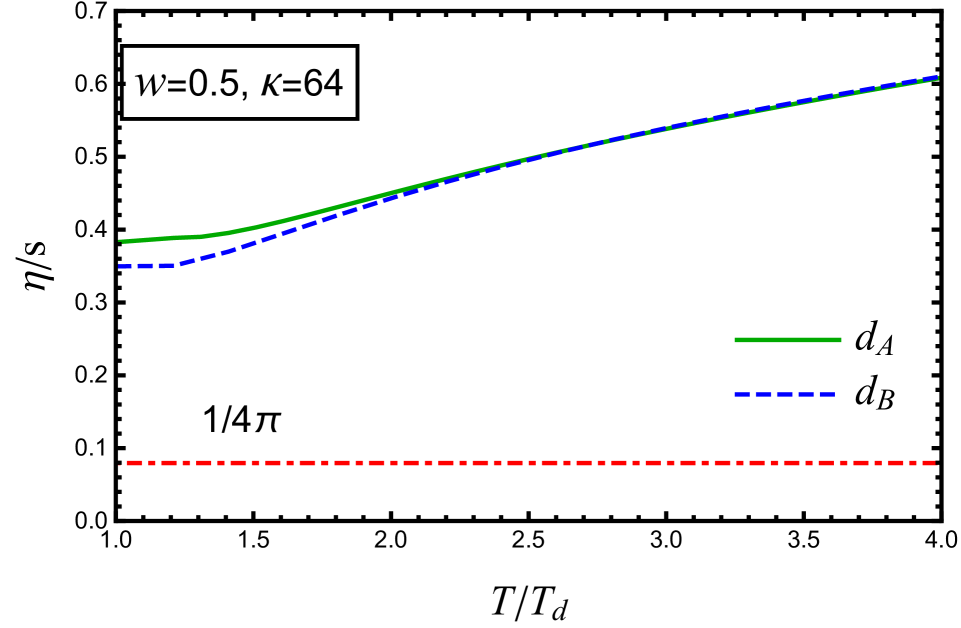
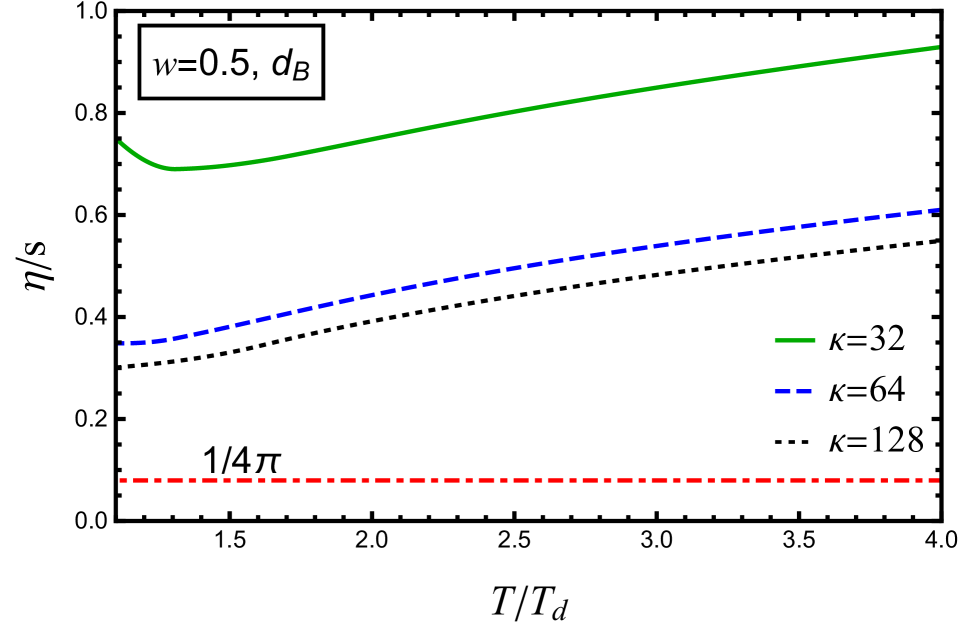
In Fig 11, we plot Eq. (161) for two ansatzes mentioned in Eq. (28). We adopt the functional form of the one-loop perturbative coupling for zero quark flavors $(N_{f}=0)$, as presented in Refs. [67, 68], to define a non-perturbative running coupling characterized by a single parameter $w$. For the running coupling, we take

$$g(T)^{2}N_{c}=4\pi\frac{6\pi}{11\log(w2\pi T/T_{d})}\;.$$ (165)

With the increasing temperature $T$, the coupling decreases, and the shear viscosity increases. With this form of the coupling constant, taking the values $w=0.5$ and $\kappa=64$, at $T_{d}$ $\eta_{\rm{pert}}/s\approx 0.55$.

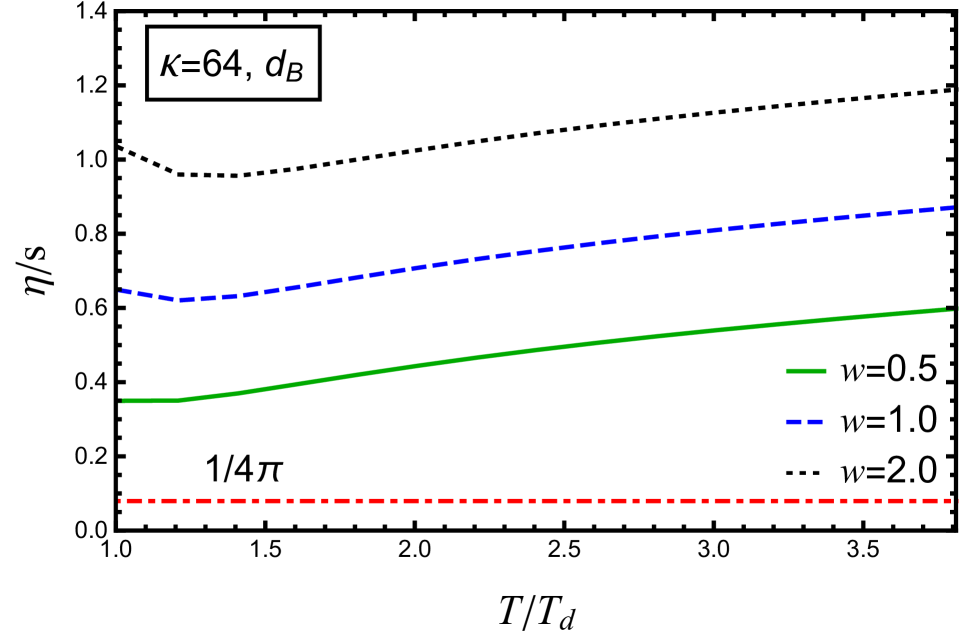
In the matrix model, how the choice of our two models is unexpectedly small, even down to $T_{d}$, and well above that in Anti-de Sitter/Conformal Field Theory, AdS/CFT [69] bound. This is illustrated in the figures with a red dash-dotted line.

The dependence of shear viscosity on the parameters $\kappa$ and $w$ are shown in Figs. 12 and 13, respectively. The former is obtained by varying $\kappa$ with a fixed value of energy scale $\pi T$ i.e., $w=0.5$. With increasing $\kappa$, the value of the viscosity reaches towards the ADS/CFT bound. These results are shown for one ansatz $d_{B}$. One will obtain a similar result for another ansatz with a marginal difference. As the QCD coupling is not well-known near the transition, we show the plots varying $w$. Figure 13 shows the results for different energy scales around $2\pi T$, i.e., for $w=0.5,1,2$.

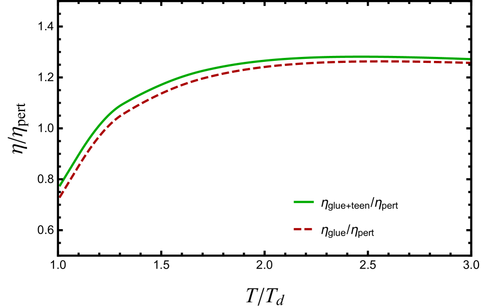
In Fig. 14, we compare our results with zero background field case. The green line represents the ratio of shear viscosity accounting for teen-teen, teen-gluon, and gluon-gluon scattering compared to gluon-gluon scattering in zero background field, whereas, the red line indicates the ratio of viscosity only including gluon-gluon scattering in presence and absence of the background fields. In the presence of background fields, these additional contributions, particularly from teens as ghost fields, lead to a rise in the overall viscosity. The inclusion of teen-teen and teen-gluon scattering contributes around $6\%$ to the viscosity near $T_{d}$.

Figure 14: The green line denotes the ratio of the shear viscosity including teen-teen, teen-gluon, and gluon-gluon scattering, to that with perturbative gluon-gluon scattering. The red-dashed line indicates the ratio of the shear viscosity including just gluon-gluon scattering, to that with perturbative. As a ghost field, the contribution with teens increases the total shear viscosity.

VI Bulk Viscosity

We next compute the bulk viscosity. While of utmost importance for phenomenology, in perturbation theory, it is more difficult to extract. The bulk viscosity vanishes for any conformal theory, so in gauge theory, it is strongly suppressed relative to the shear viscosity. As shown by Arnold, Dugan, and Moore [46], the bulk viscosity only arises because quarks and gluons develop a thermal “mass” $\sim gT$. Even then, it is necessary to include the running of the coupling constant with temperature. Consequently, the bulk viscosity is suppressed by $\sim g^{8}$ and is $\zeta\sim g^{4}$, relative to the shear viscosity, $\eta\sim 1/g^{4}$.

In contrast, in our matrix model the theory is not conformally invariant if the Polyakov loops are less than unity, since then there must be a non-trivial distribution for the eigenvalues of the thermal Wilson line. Thus while in perturbation theory it is involved to measure the deviation from conformality through the bulk viscosity, in our matrix model it is straightforward. In particular, we can compute in precisely the same way as for the shear viscosity, to leading logarithmic order in the coupling constant. As we show, the bulk viscosity is nonzero because the speed of sound squared is not equal to $1/3$; i.e., the theory is not conformal.

For the bulk viscosity, from Eq. (102),

$$2P^{\mu,a_{1}b_{1}}\partial_{\mu}^{(1)}f_{\text{\bngx b},a_{1}b_{1}}=\beta f^{0}_{a_{1}b_{1}}(1+f^{0}_{a_{1}b_{1}})\mathrm{X}q(|{\bf\it p}|)\;,$$ (166)

where

$$\mathrm{X}=\nabla\cdot\bm{u}\;,$$ (167)

and

$$q(p)=2p^{2}\quantity(\frac{1}{3}-v_{s}^{2})\equiv 2p^{2}\Delta v_{s}^{2}\;,$$ (168)

with $v_{s}^{2}$ the speed of sound, squared, Eq. (103). In a conformally invariant theory $v_{s}^{2}=1/3$ and the bulk viscosity vanishes. In our matrix model, the dominant source of conformal symmetry breaking is from $v_{s}^{2}\neq 1/3$ as discussed below.

We expand the statistical distribution functions to linear order,

$$f^{(n)}_{\text{\bngx b},ab}=\ f^{0}_{ab}\;(1+f^{0}_{ab})\psi_{\text{\bngx b},ab}^{(n)}\;.$$ (169)

Analogous to Eq. (106), then, the Boltzmann equation is written as

$$\beta f^{0}_{a_{1}b_{1}}(1+f^{0}_{a_{1}b_{1}})\mathrm{X}q(|{\bf\it p}|)=-{\mathcal{S}}_{\text{\bngx b}}(\bar{\mathcal{L}}\psi^{(1)})_{\text{\bngx b},a_{1}b_{1}}\;,$$ (170)

where $\bar{\mathcal{L}}$ is a linear operator,

$$(\bar{\mathcal{L}}\psi^{(n)})_{\text{\bngx b},a_{1}b_{1}}=\frac{1}{2}\sum_{\text{\bngx d},\text{\bngx b}^{\prime},\text{\bngx d}^{\prime}}{\mathcal{S}}_{\text{\bngx b}}{\mathcal{S}}_{\text{\bngx d}}\int_{\text{\bngx d}}d\Gamma_{a_{2}b_{2}}\,\int_{\text{\bngx b}^{\prime}}d\Gamma_{a_{3}b_{3}}\,\int_{\text{\bngx d}^{\prime}}d\Gamma_{a_{4}b_{4}}\,(2\pi)^{4}\delta^{(4)}(P^{a_{1}b_{1}}_{1}+P^{a_{2}b_{2}}_{2}-P^{a_{3}b_{3}}_{3}-P^{a_{4}b_{4}}_{4})$$

$$\;\;\;\;\;\;\;\;\;\times|\mathcal{M}_{\text{\bngx b}\text{\bngx d}\rightarrow\text{\bngx b}^{\prime}\text{\bngx d}^{\prime}}|^{2}\bigg{[}f_{a_{1}b_{1}}^{0}f_{a_{2}b_{2}}^{0}(1+f_{a_{3}b_{3}}^{0})(1+f_{a_{4}b_{4}}^{0})\bigg{]}\bigg{(}\psi_{\text{\bngx b},a_{1}b_{1}}^{(n)}+\psi_{\text{\bngx d},a_{2}b_{2}}^{(n)}-\psi_{\text{\bngx b}^{\prime},a_{3}b_{3}}^{(n)}-\psi_{\text{\bngx d}^{\prime},a_{4}b_{4}}^{(n)}\bigg{)}\;.$$ (171)

Here, the operator $\bar{\mathcal{L}}$ is the same as ${\mathcal{L}}$ in Eq. (V.2), with the bar added to emphasize its role in describing the bulk viscosity.

The bulk viscosity is defined by the change in pressure caused by the deviation from equilibrium $\psi_{\text{\bngx b}}$. The bulk viscosity, $\zeta$, is given by [46]

$$\zeta = -\sum_{\text{\bngx b}}{\mathcal{S}}_{\text{\bngx b}}\;\int_{\text{\bngx b}}d\Gamma_{a_{1}b_{1}}\,q(|{\bf\it p}|)f^{0}_{a_{1}b_{1}}(1+f^{0}_{a_{1}b_{1}})\psi_{\text{\bngx b}}(p)\;.$$ (172)

The source term, $f^{0}_{a_{1}b_{1}}(1+f^{0}_{a_{1}b_{1}})q(|{\bf\it p}|)$, in Eq. (170) can be written in terms of an expansion basis as

$$V_{\text{\bngx b},n}={\mathcal{S}}_{\text{\bngx b}}\;\int_{\text{\bngx b}}d\Gamma_{a_{1}b_{1}}\,2p^{2}\psi^{\text{\bngx b}}_{n}\beta f^{0}_{a_{1}b_{1}}(1+f^{0}_{a_{1}b_{1}})\,\Delta v_{s}^{2}\;,$$ (173)

giving us $V_{\text{\bngx b},n}=-(\bar{\mathcal{L}}\bar{c})_{n}^{\text{\bngx b}}$. Here, we expanded $\psi^{\text{\bngx b}}$ in an orthogonal basis equivalent to Eq. (112) as $\psi^{\text{\bngx d}}=\sum_{n}\bar{c}_{n}^{\text{\bngx d}}\psi^{\text{\bngx d}}_{n}$. Finally, the coefficient of bulk viscosity from Eq. (172) becomes

$$\zeta = T\sum_{\text{\bngx b}}\;\int_{\text{\bngx b}}d\Gamma_{a_{1}b_{1}}\psi_{\text{\bngx b}}(\bar{\mathcal{L}}\psi)_{\text{\bngx b}}$$ (174)

$$= T\sum_{\text{\bngx b}}\sum_{n=0}^{\infty}V_{n}^{\text{\bngx b}}\big{(}\bar{\mathcal{L}}^{-1}V\big{)}_{n}^{\text{\bngx b}}=T\sum_{\text{\bngx b}}\sum_{n=0}^{\infty}\bar{c}_{n}^{\text{\bngx b}}(\bar{\mathcal{L}}\bar{c})_{n}^{\text{\bngx b}}\;.$$

In Appendix B, we show that if one computes the pressure for a teen field from kinetic theory, then one obtains $\mathscr{P}_{\rm teen}=-T^{2}T_{d}^{2}/72$, with the energy $\mathscr{E}=-T^{2}T_{d}^{2}/24$. That is, in kinetic theory teen quasiparticles still look three-dimensional, with $\mathscr{E}=\mathscr{P}_{\rm teen}$. In Appendix B, we argue how a kinetic theory of two dimensional teen particles can arise, with $\mathscr{E}=\mathscr{P}_{\rm teen}=-T^{2}T_{d}^{2}/24$  [43], as in thermodynamics.

In practice, we define our model such that in Eq. (174), the deviation from conformality, $\Delta v_{s}^{2}$, is computed from thermodynamics. After all, in our model the teen fields are not really two-dimensional, but defined with the functions $d_{A}(T)$ and $d_{B}(T)$, which are fit to obtain $(\mathscr{E}-3\mathscr{P})/T^{4}$ from the lattice, Eq. (28). Except for the contribution to $\Delta v_{s}^{2}$, though, we compute Eq. (174) using gluon and teen quasiparticles in the semi-QGP. We believe that this ansatz yields a reasonable estimate of the bulk viscosity.

With this assumption, following Ref. [46], we use a simple ansatz for the basis functions, $\psi^{\mathrm{g}}$,

$$\psi_{m}^{\mathrm{g}}=\frac{T}{(1+p/T)^{K-2}}\;\left(\frac{p}{T}\right)^{m},\qquad m=1,2,\cdots,K\;.$$ (175)

Here, the $\psi^{\mathrm{g}}_{m}$ are not necessarily orthogonal. We take a different basis for the $\psi^{\text{\bngx 3}}_{m}$ as

$$\psi_{m}^{\text{\bngx 3}}=\frac{T}{(1+p/T)^{K-4}}\;\left(\frac{p}{T}\right)^{m}\;,\qquad m=1,2,\cdots,K\;.$$ (176)

By trial and error, we found that a different basis for the teen functions, Eq. (176), converges more quickly (at $K\sim 35$) than if we take the same basis as for gluons, Eq. (175).

For a single order basis, i.e., $K=1$, we get

$$V_{\mathrm{g},1} = 2(\Delta v_{s}^{2})\ \frac{24T^{4}}{2\pi^{2}}\sum_{k=1}^{\infty}\frac{N_{c}^{2}\ell_{k}^{2}-1}{k^{5}}(5+k)\;,$$ (177)

$$V_{\text{\bngx 3},1} = -(\Delta v_{s}^{2})\ \frac{T^{2}T_{d}^{2}}{4\pi^{2}}\sum_{k=1}^{\infty}\frac{N_{c}^{2}\ell_{k}^{2}-1}{k^{5}}(60+36k+9k^{2}+k^{3})\;.$$ (178)

Beyond $K=1$, it is also necessary to treat the zero modes in the operator for the bulk viscosity. This is discussed in Appendix C.

VI.1 Matrix Element at Leading log

Analogous to Eq. (131), the matrix element form for the b-d scattering becomes

$$\bar{\Lambda}^{\text{\bngx b},\text{\bngx d}}_{mn} =\left(2\frac{1}{4}\right)\frac{1}{2}{\mathcal{S}}_{\text{\bngx b}}{\mathcal{S}}_{\text{\bngx d}}\int_{\text{\bngx b}}d\Gamma_{{a_{1}b_{1}}}\int_{\text{\bngx d}}d\Gamma_{a_{2}b_{2}}\,\int_{\text{\bngx b}}d\Gamma_{a_{3}b_{3}}\,\int_{\text{\bngx d}}d\Gamma_{a_{4}b_{4}}$$ (179)

$$\times(2\pi)^{4}\delta^{(4)}(P^{a_{1}b_{1}}_{1}+P^{a_{2}b_{2}}_{2}-P^{a_{3}b_{3}}_{3}-P^{a_{4}b_{4}}_{4})|\mathcal{M}_{\text{\bngx b}\text{\bngx d}\rightarrow\text{\bngx b}\text{\bngx d}}|^{2}f_{a_{1}b_{1}}^{0}f_{a_{2}b_{2}}^{0}\big{(}1+f_{a_{3}b_{3}}^{0}\big{)}\big{(}1+f_{a_{4}b_{4}}^{0}\big{)}$$

$$\times\left[(\psi_{1}^{\text{\bngx b},m}-\psi_{3}^{\text{\bngx b},m})\bar{c}_{n}^{\text{\bngx b}}+(\psi_{2}^{\text{\bngx d},m}-\psi_{4}^{\text{\bngx d},m})\bar{c}_{n}^{\text{\bngx d}}\right]\left[(\psi_{1}^{\text{\bngx b},n}-\psi_{3}^{\text{\bngx b},n})\bar{c}_{m}^{\text{\bngx b}}+(\psi_{2}^{\text{\bngx d},n}-\psi_{4}^{\text{\bngx d},n})\bar{c}_{m}^{\text{\bngx d}}\right]\;.$$

If the momentum transfer in the scattering process is small, we get

$$\psi^{\text{\bngx b}}_{1}-\psi^{\text{\bngx b}}_{3}\simeq{\bf\it k}\cdot\partial_{{\bf\it p}}\psi^{\text{\bngx b}}(p)\;,\quad\psi^{\text{\bngx b}}_{2}-\psi^{\text{\bngx b}}_{4}\simeq-{\bf\it k}\cdot\partial_{{\bf\it p}^{\prime}}\psi^{\text{\bngx b}}(p^{\prime})\;,$$ (180)

where we have used ${\bf\it p}\equiv({{\bf\it p}_{1}+{\bf\it p}_{3}})/{2}$ and ${\bf\it p}^{\prime}\equiv({{\bf\it p}_{2}+{\bf\it p}_{4}})/{2}$, $x\equiv{k_{0}}/{k}\simeq\cos\theta_{\bm{pk}}\simeq\cos\theta_{\bm{p^{\prime}k}}$ from Eqs. (65)-(67). In the small momentum transfer limit, the matrix element from Eq. (179) becomes

$$\bar{\Lambda}^{\text{\bngx b},\text{\bngx d}}_{mn} = 2\frac{g^{4}}{(2\pi)^{5}}\frac{\sigma_{\text{\bngx b}}\sigma_{\text{\bngx d}}}{4}{\mathcal{S}}_{\text{\bngx b}}{\mathcal{S}}_{\text{\bngx d}}\prod_{i=1}^{4}\sum_{a_{i},b_{i}}\sum_{n_{1},n_{2}=1}^{\infty}\sum_{n_{3},n_{4}=0}^{\infty}\mathcal{G}(Q,n_{1},\cdots,n_{4})t^{ab}_{13}\,t^{ba}_{24}\,t^{cd}_{13}\,t^{dc}_{24}\,\int_{0}^{\infty}dp\,p^{2}e^{-\beta p(n_{1}+n_{3})}$$ (181)

$$\times\int_{0}^{\infty}dp^{\prime}\,p^{\prime 2}\,e^{-\beta p^{\prime}(n_{2}+n_{4})}\int_{0}^{2\pi}\frac{d\phi}{2\pi}\,\int_{-1}^{1}dx\,\int_{0}^{\infty}dk\,k^{3}\,|D_{L}^{ab}(K)+(1-x^{2})\cos\phi\,D_{T}^{ab}(K)|^{2}$$

$$\times\left[\bar{c}_{m}^{\text{\bngx b}}\,\hat{\bm{k}}\cdot\partial_{{\bf\it p}}\psi^{\text{\bngx b},m}(p)-\bar{c}_{m}^{\text{\bngx d}}\,\hat{\bm{k}}\cdot\partial_{{\bf\it p}^{\prime}}\psi^{\text{\bngx d},m}(p^{\prime})\right]\left[\bar{c}_{n}^{\text{\bngx b}}\,\hat{\bm{k}}\cdot\partial_{{\bf\it p}}\psi^{\text{\bngx b},n}(p)-\bar{c}_{n}^{\text{\bngx d}}\,\hat{\bm{k}}\cdot\partial_{{\bf\it p}^{\prime}}\psi^{\text{\bngx d},n}(p^{\prime})\right]\;.$$

Here, $\sigma_{\text{\bngx b}}$ represents the spin degeneracy; $\sigma_{\mathrm{g}}=2$ and $\sigma_{\text{\bngx 3}}=1$. We assume rotational invariance, $\psi^{\text{\bngx b},n}({\bf\it p})=\psi^{\text{\bngx b},n}(p)$, so that

$$\left[\bar{c}_{m}^{\text{\bngx b}}\,\hat{\bm{k}}\cdot\partial_{{\bf\it p}}\psi^{\text{\bngx b},m}(p)-\bar{c}_{m}^{\text{\bngx d}}\,\hat{\bm{k}}\cdot\partial_{{\bf\it p}^{\prime}}\psi^{\text{\bngx d},m}(p^{\prime})\right]=x\left[\bar{c}_{m}^{\text{\bngx b}}\,(\psi_{m}^{\text{\bngx b}})^{{}^{\prime}}(p)-\bar{c}_{m}^{\text{\bngx d}}\,(\psi_{m}^{\text{\bngx d}})^{{}^{\prime}}(p^{\prime})\right]\;.$$ (182)

Hence, using Eq. (182) we can rewrite Eq. (181) as

$$\bar{\Lambda}^{\text{\bngx b},\text{\bngx d}}_{mn} = \frac{g^{4}}{(2\pi)^{5}}\frac{\sigma_{\text{\bngx b}}\sigma_{\text{\bngx d}}}{4}\log\left(\frac{\kappa}{g^{2}N_{c}}\right){\mathcal{S}}_{\text{\bngx b}}{\mathcal{S}}_{\text{\bngx d}}\prod_{i=1}^{4}\sum_{a_{i},b_{i}}\sum_{n_{1},n_{2}=1}^{\infty}\sum_{n_{3},n_{4}=0}^{\infty}\mathcal{G}(Q,n_{1},\cdots,n_{4})t^{ab}_{13}\,t^{ba}_{24}\,t^{cd}_{13}\,t^{dc}_{24}$$ (183)

$$\times\int_{0}^{\infty}dp\,p^{2}\,e^{-\beta p(n_{1}+n_{3})}\int_{0}^{\infty}dp^{\prime}\,p^{\prime 2}\,e^{-\beta p^{\prime}(n_{2}+n_{4})}\int_{0}^{2\pi}\frac{d\phi}{2\pi}\left(1-\cos\phi\right)^{2}\int_{-1}^{1}dx\,x^{2}\,$$

$$\times\left[\bar{c}_{m}^{\text{\bngx b}}\,(\psi_{m}^{\text{\bngx b}})^{{}^{\prime}}(p)-\bar{c}_{m}^{\text{\bngx d}}\,(\psi_{m}^{\text{\bngx d}})^{{}^{\prime}}(p^{\prime})\right]\left[\bar{c}_{n}^{\text{\bngx b}}\,(\psi_{n}^{\text{\bngx b}})^{{}^{\prime}}(p)-\bar{c}_{n}^{\text{\bngx d}}\,(\psi_{n}^{\text{\bngx d}})^{{}^{\prime}}(p^{\prime})\right]$$

$$= \frac{g^{4}}{(2\pi)^{5}}\frac{\sigma_{\text{\bngx b}}\sigma_{\text{\bngx d}}}{4}\log\left(\frac{\kappa}{g^{2}N_{c}}\right){\mathcal{S}}_{\text{\bngx b}}{\mathcal{S}}_{\text{\bngx d}}\prod_{i=1}^{4}\sum_{a_{i},b_{i}}\sum_{n_{1},n_{2}=1}^{\infty}\sum_{n_{3},n_{4}=0}^{\infty}\mathcal{G}(Q,n_{1},\cdots,n_{4})t^{ab}_{13}\,t^{ba}_{24}\,t^{cd}_{13}\,t^{dc}_{24}$$

$$\times\int_{0}^{\infty}dp\,p^{2}\,e^{-\beta p(n_{1}+n_{3})}\int_{0}^{\infty}dp^{\prime}\,p^{\prime 2}\,e^{-\beta p^{\prime}(n_{2}+n_{4})}\left[\bar{c}_{m}^{\text{\bngx b}}\,(\psi_{m}^{\text{\bngx b}})^{{}^{\prime}}(p)-\bar{c}_{m}^{\text{\bngx d}}\,(\psi_{m}^{\text{\bngx d}})^{{}^{\prime}}(p^{\prime})\right]$$

$$\times\left[\bar{c}_{n}^{\text{\bngx b}}\,(\psi_{n}^{\text{\bngx b}})^{{}^{\prime}}(p)-\bar{c}_{n}^{\text{\bngx d}}\,(\psi_{n}^{\text{\bngx d}})^{{}^{\prime}}(p^{\prime})\right]$$

$$= \frac{g^{4}}{(2\pi)^{5}}\frac{\sigma_{\text{\bngx b}}\sigma_{\text{\bngx d}}}{4}\log\left(\frac{\kappa}{g^{2}N_{c}}\right){\mathcal{S}}_{\text{\bngx b}}{\mathcal{S}}_{\text{\bngx d}}\sum_{m_{1},m_{2}=1}^{\infty}\sum_{m_{3}=1}^{m_{1}}\sum_{m_{4}=1}^{m_{2}}\frac{N_{c}^{4}}{2}\ell_{m_{1}}\ell_{m_{2}}(\ell_{m_{1}-m_{2}-m_{3}+m_{4}}\ell_{m_{4}-m_{3}}$$

$$+\ell_{m_{1}-m_{3}+m_{4}}\ell_{m_{2}+m_{3}-m_{4}})\int_{0}^{\infty}dp\,p^{2}\,e^{-\beta pm_{1}}\int_{0}^{\infty}dp^{\prime}\,p^{\prime 2}\,e^{-\beta p^{\prime}m_{2}}$$

$$\times\left[\bar{c}_{m}^{\text{\bngx b}}\,(\psi_{m}^{\text{\bngx b}})^{{}^{\prime}}(p)-\bar{c}_{m}^{\text{\bngx d}}\,(\psi_{m}^{\text{\bngx d}})^{{}^{\prime}}(p^{\prime})\right]\left[\bar{c}_{n}^{\text{\bngx b}}\,(\psi_{n}^{\text{\bngx b}})^{{}^{\prime}}(p)-\bar{c}_{n}^{\text{\bngx d}}\,(\psi_{n}^{\text{\bngx d}})^{{}^{\prime}}(p^{\prime})\right].$$

Here we have used the color sum in the limit of large $N_{c}$ and it becomes

$$\prod_{i=1}^{4}\sum_{a_{i},b_{i}}t^{ab}_{13}\,t^{ba}_{24}\,t^{cd}_{13}\,t^{dc}_{24}\mathcal{G}(Q,n_{1},\cdots,n_{4})$$

$$=\frac{N_{c}^{4}}{2}\ell_{n_{1}+n_{3}}\ell_{n_{2}+n_{4}}(\ell_{n_{2}-n_{1}}\ell_{n_{4}-n_{3}}+\ell_{n_{1}+n_{4}}\ell_{n_{2}+n_{3}})\;,$$ (184)

with $m_{1}\equiv n_{1}+n_{3}$, $m_{2}\equiv n_{2}+n_{4}$, $m_{3}\equiv n_{3}$, $m_{4}\equiv n_{4}$.

VI.1.1 Gluon-gluon scattering

For the gluon-gluon scattering, at nonzero holonomy, the matrix element from Eq. (183) becomes

$$\bar{\Lambda}^{\mathrm{gg}}_{mn} = \frac{g^{4}N_{c}^{4}}{2(2\pi)^{5}}\log\left(\frac{\kappa}{g^{2}N_{c}}\right)\sum_{m_{1},m_{2}=1}^{\infty}\sum_{m_{3}=1}^{m_{1}}\sum_{m_{4}=1}^{m_{2}}\,\ell_{m_{1}}\ell_{m_{2}}\;\ell_{m_{1},m_{2},m_{3},m_{4}}\;\int_{0}^{\infty}dp\,p^{2}$$ (185)

$$\times\int_{0}^{\infty}dp^{\prime}\,p^{\prime 2}\text{e}^{-\beta(m_{1}p+m_{2}p^{\prime})}\bar{c}_{m}^{\mathrm{g}}\bar{c}_{n}^{\mathrm{g}}[(\psi^{\mathrm{g}}_{m}(p))^{\prime}-(\psi^{\mathrm{g}}_{m}(p^{\prime}))^{\prime}][(\psi^{\mathrm{g}}_{n}(p))^{\prime}-(\psi^{\mathrm{g}}_{n}(p^{\prime}))^{\prime}]$$

$$= \frac{g^{4}N_{c}^{4}}{2(2\pi)^{5}}\log\left(\frac{\kappa}{g^{2}N_{c}}\right)\bar{c}_{m}^{\mathrm{g}}\bar{c}_{n}^{\mathrm{g}}T^{6}\,Y^{\mathrm{gg}}_{mn}\;,$$

where, $\ell_{m_{1},m_{2},m_{3},m_{4}}$ is defined in Eq. (145) and we define

$$Y^{\mathrm{gg}}_{mn} = \frac{1}{T^{6}}\sum_{m_{1},m_{2}=1}^{\infty}\sum_{m_{3}=1}^{m_{1}}\sum_{m_{4}=1}^{m_{2}}\,\ell_{m_{1}}\ell_{m_{2}}\;\ell_{m_{1},m_{2},m_{3},m_{4}}\;\int_{0}^{\infty}p^{2}dp$$ (186)

$$\times \int_{0}^{\infty}(p^{\prime})^{2}dp^{\prime}\text{e}^{-\beta(m_{1}p+m_{2}p^{\prime})}[(\psi^{\mathrm{g}}_{m}(p))^{\prime}-(\psi^{\mathrm{g}}_{m}(p^{\prime}))^{\prime}][(\psi^{\mathrm{g}}_{n}(p))^{\prime}-(\psi^{\mathrm{g}}_{n}(p^{\prime}))^{\prime}]\;.$$

The factors related to temperature and the coupling constant remain consistent with those found in the perturbative Quark-Gluon Plasma (QGP) framework. The function $Y^{\mathrm{gg}}_{nm}$ encapsulates all the modifications or effects introduced by the background field in the system’s behavior or properties. The diagram that plays a role in the contributions to the calculation is shown in Fig. 9a.

VI.1.2 Gluon-teen scattering

Analogous to the gluon-gluon scattering, the matrix element for gluon-teen scattering at nonzero holonomy is

$$\bar{\Lambda}^{\mathrm{g}\text{\bngx 3}}_{mn} = -\frac{1}{2}\frac{g^{4}N_{c}^{4}}{2(2\pi)^{5}}\log\left(\frac{\kappa}{g^{2}N_{c}}\right)\sum_{m_{1},m_{2}=1}^{\infty}\sum_{m_{3}=1}^{m_{1}}\sum_{m_{4}=1}^{m_{2}}\ell_{m_{1}}\ell_{m_{2}}\;\ell_{m_{1},m_{2},m_{3},m_{4}}\frac{T_{d}^{2}}{2}\int_{0}^{\infty}dp\,$$ (187)

$$\hskip-25.6073pt\times\int_{0}^{\infty}dp^{\prime}\,p^{\prime 2}\text{e}^{-\beta(m_{1}p+m_{2}p^{\prime})}[\bar{c}_{m}^{\text{\bngx 3}}\,(\psi^{\text{\bngx 3}}_{m}(p))^{\prime}-\bar{c}_{m}^{\mathrm{g}}(\psi^{\mathrm{g}}_{m}(p^{\prime}))^{\prime}][\bar{c}_{n}^{\text{\bngx 3}}(\psi^{\text{\bngx 3}}_{n}(p))^{\prime}-\bar{c}_{n}^{\mathrm{g}}(\psi^{\mathrm{g}}_{n}(p^{\prime}))^{\prime}]$$

$$= \frac{g^{4}N_{c}^{4}}{2(2\pi)^{5}}\log\left(\frac{\kappa}{g^{2}N_{c}}\right)T^{4}T_{d}^{2}(\bar{c}_{m}^{\mathrm{g}}\bar{c}_{n}^{\mathrm{g}}\overline{Y}^{\mathrm{gg}}_{mn}+\bar{c}_{m}^{\text{\bngx 3}}\bar{c}_{n}^{\text{\bngx 3}}\overline{Y}^{\text{\bngx 3}\text{\bngx 3}}_{mn}-\bar{c}_{m}^{\mathrm{g}}\bar{c}_{n}^{\text{\bngx 3}}Y^{\mathrm{g}\text{\bngx 3}}_{mn}-\bar{c}_{m}^{\text{\bngx 3}}\bar{c}_{n}^{\mathrm{g}}Y^{\text{\bngx 3}\mathrm{g}}_{mn})\;,$$

with $\ell_{m_{1},m_{2},m_{3},m_{4}}$ given in Eq. (145) and

$$\overline{Y}^{\mathrm{gg}}_{mn} = -\frac{1}{2}\frac{1}{T^{4}}\sum_{m_{1},m_{2}=1}^{\infty}\sum_{m_{3}=1}^{m_{1}}\sum_{m_{4}=1}^{m_{2}}\,\ell_{m_{1}}\ell_{m_{2}}\;\ell_{m_{1},m_{2},m_{3},m_{4}}\;$$

$$\times \frac{1}{2}\int_{0}^{\infty}dp\int_{0}^{\infty}(p^{\prime})^{2}dp^{\prime}\text{e}^{-\beta(m_{1}p+m_{2}p^{\prime})}(\psi^{\mathrm{g}}_{m}(p^{\prime}))^{\prime}(\psi^{\mathrm{g}}_{n}(p))^{\prime}\;,$$

$$\overline{Y}^{\mathrm{g}\text{\bngx 3}}_{mn} = -\frac{1}{2}\frac{1}{T^{4}}\sum_{m_{1},m_{2}=1}^{\infty}\sum_{m_{3}=1}^{m_{1}}\sum_{m_{4}=1}^{m_{2}}\,\ell_{m_{1}}\ell_{m_{2}}\;\ell_{m_{1},m_{2},m_{3},m_{4}}\;$$

$$\times \frac{1}{2}\int_{0}^{\infty}dp\int_{0}^{\infty}(p^{\prime})^{2}dp^{\prime}\text{e}^{-\beta(m_{1}p+m_{2}p^{\prime})}(\psi^{\mathrm{g}}_{m}(p^{\prime}))^{\prime}(\psi^{\text{\bngx 3}}_{n}(p))^{\prime}\;,$$

$$\overline{Y}^{\text{\bngx 3}\mathrm{g}}_{mn} = -\frac{1}{2}\frac{1}{T^{4}}\sum_{m_{1},m_{2}=1}^{\infty}\sum_{m_{3}=1}^{m_{1}}\sum_{m_{4}=1}^{m_{2}}\,\ell_{m_{1}}\ell_{m_{2}}\;\ell_{m_{1},m_{2},m_{3},m_{4}}\;$$

$$\times \frac{1}{2}\int_{0}^{\infty}dp\int_{0}^{\infty}(p^{\prime})^{2}dp^{\prime}\text{e}^{-\beta(m_{1}p+m_{2}p^{\prime})}(\psi^{\text{\bngx 3}}_{m}(p^{\prime}))^{\prime}(\psi^{\mathrm{g}}_{n}(p))^{\prime}\;,$$

$$\overline{Y}^{\text{\bngx 3}\text{\bngx 3}}_{mn} = -\frac{1}{2}\frac{1}{T^{4}}\sum_{m_{1},m_{2}=1}^{\infty}\sum_{m_{3}=1}^{m_{1}}\sum_{m_{4}=1}^{m_{2}}\,\ell_{m_{1}}\ell_{m_{2}}\;\ell_{m_{1},m_{2},m_{3},m_{4}}\;$$ (188)

$$\times \frac{1}{2}\int_{0}^{\infty}dp\int_{0}^{\infty}(p^{\prime})^{2}dp^{\prime}\text{e}^{-\beta(m_{1}p+m_{2}p^{\prime})}(\psi^{\text{\bngx 3}}_{m}(p^{\prime}))^{\prime}(\psi^{\text{\bngx 3}}_{n}(p))^{\prime}\;.$$

The contributing diagram is presented in Fig. 9b.

VI.1.3 Teen-Teen scattering

The matrix element for teen-teen scattering is

$$\bar{\Lambda}^{\text{\bngx 3}\text{\bngx 3}}_{mn} = \frac{1}{4}\frac{g^{4}N_{c}^{4}}{2(2\pi)^{5}}\log\left(\frac{\kappa}{g^{2}N_{c}}\right)\sum_{m_{1},m_{2}=1}^{\infty}\sum_{m_{3}=1}^{m_{1}}\sum_{m_{4}=1}^{m_{2}}\ell_{m_{1}}\ell_{m_{2}}\;\ell_{m_{1},m_{2},m_{3},m_{4}}\frac{T_{d}^{2}}{2}\int_{0}^{\infty}dp\,$$ (189)

$$\times\frac{T_{d}^{2}}{2}\int_{0}^{\infty}dp^{\prime}\,\,e^{-\beta(m_{1}p+m_{2}p^{\prime})}\bar{c}_{m}^{\text{\bngx 3}}\bar{c}_{n}^{\text{\bngx 3}}[(\psi^{\text{\bngx 3}}_{m}(p))^{\prime}-(\psi^{\text{\bngx 3}}_{m}(p^{\prime}))^{\prime}][(\psi^{\text{\bngx 3}}_{n}(p))^{\prime}-(\psi^{\text{\bngx 3}}_{n}(p^{\prime}))^{\prime}]\;$$

$$= \frac{g^{4}N_{c}^{4}}{2(2\pi)^{5}}\log\left(\frac{\kappa}{g^{2}N_{c}}\right)\bar{c}_{m}^{\text{\bngx 3}}\bar{c}_{n}^{\text{\bngx 3}}T_{d}^{4}T^{2}Y^{\text{\bngx 3}\text{\bngx 3}}_{mn}\;,$$

where

$$Y^{\text{\bngx 3}\text{\bngx 3}}_{mn} = \frac{1}{4}\frac{1}{T^{2}}\sum_{m_{1},m_{2}=1}^{\infty}\sum_{m_{3}=1}^{m_{1}}\sum_{m_{4}=1}^{m_{2}}\,\ell_{m_{1}}\ell_{m_{2}}\;\ell_{m_{1},m_{2},m_{3},m_{4}}\;$$ (190)

$$\times \frac{1}{2}\int_{0}^{\infty}dp\frac{1}{2}\int_{0}^{\infty}dp^{\prime}\text{e}^{-\beta(m_{1}p+m_{2}p^{\prime})}(\psi^{\text{\bngx 3}}_{m}(p^{\prime}))^{\prime}(\psi^{\text{\bngx 3}}_{n}(p))^{\prime}\;.$$

Adding up the matrix elements from gluon-gluon, gluon-teen, and teen-teen scattering, one can rewrite the total matrix element as

$$\sum_{\text{\bngx b},n}\bar{c}_{n}^{\text{\bngx b}}(\bar{\mathcal{L}}\bar{c})_{n}^{\text{\bngx b}} \simeq \frac{g^{4}N_{c}^{4}}{2(2\pi)^{5}}\log\left(\frac{\kappa}{g^{2}N_{c}}\right)$$ (191)

$$\hskip-28.45274pt\times\sum_{m,n=1}^{K}\begin{bmatrix}\bar{c}_{m}^{\mathrm{g}}&\bar{c}_{m}^{\text{\bngx 3}}\end{bmatrix}\begin{bmatrix}T^{6}{Y}^{\mathrm{gg}}_{mn}+T^{4}\,T_{d}^{2}{\overline{Y}}^{\mathrm{gg}}_{mn}&-T^{4}\,T_{d}^{2}{Y}^{\mathrm{g}\text{\bngx 3}}_{mn}\\ -T^{4}\,T_{d}^{2}{Y}^{\text{\bngx 3}\mathrm{g}}_{mn}&T_{d}^{4}\,T^{2}{Y}^{\text{\bngx 3}\text{\bngx 3}}_{mn}+T^{4}\,T_{d}^{2}{\overline{Y}}^{\text{\bngx 3}\text{\bngx 3}}_{mn}\end{bmatrix}\begin{bmatrix}\bar{c}_{n}^{\mathrm{g}}\\ \bar{c}_{n}^{\text{\bngx 3}}\end{bmatrix}\;.$$

It is worth commenting about the terms from gluon-teen scattering in this expression. Naively, one might expect that the only contribution to the glue-glue term, $\bar{c}_{m}^{\mathrm{g}}\bar{c}_{n}^{\mathrm{g}}$, is from glue-glue scattering. This is incorrect, since Eq. (183), there are terms $\sim\bar{c}^{\text{\bngx b}}\bar{c}^{\text{\bngx d}}$, where b and d can be either a gluon or a teen field. Hence gluon-teen scattering contributes to $\bar{c}_{m}^{\mathrm{g}}\bar{c}_{n}^{\mathrm{g}}$ term, through the term ${\overline{Y}}^{\mathrm{gg}}_{mn}$. Similarly, for the $\bar{c}_{m}^{\text{\bngx 3}}\bar{c}_{n}^{\text{\bngx 3}}$ term, there are terms from gluon-teen scattering, $\sim{\overline{Y}}^{\text{\bngx 3}\text{\bngx 3}}_{mn}$.

Because the scattering kernel in Eq. (191) has zero modes, it is necessary to add an additional term to compute the bulk viscosity. We discuss these details in Appendix (C).

VI.2 Results for the Bulk Viscosity

We first compute $\zeta$ for small values of the loop. Neglecting higher powers of the first loop, $\ell_{1}$, and higher loops, $\ell_{n}$ for $n\geq 2$,

$$\zeta\approx 68.035\frac{(\Delta v_{s}^{2})^{2}\;T^{3}}{g^{4}\ln({\kappa}/{g^{2}N_{c}})}\ell_{1}^{2}\;.$$ (192)

Note, however, that in the pure glue theory the Polyakov loops are never small: near $T_{d}$, $\langle\ell_{1}\rangle\approx 0.5$ at $N_{c}=\infty$, and $\langle\ell_{1}\rangle\approx 0.4$ for $N_{c}=3$.

The entropy density $s(T)$ and $\Delta v_{s}^{2}$ are calculated using Eq. (27), i.e., lattice pressure for three colors [54].

Figure 15: Ratio of the bulk viscosity to the entropy density with the ansatz of Eq. (28), with the parameters $w=0.5$ and $\kappa=64$. The dot-dashed line corresponds to the result in a Gribov-Zwanziger model [70].

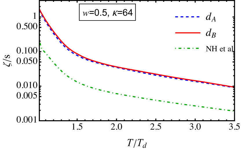
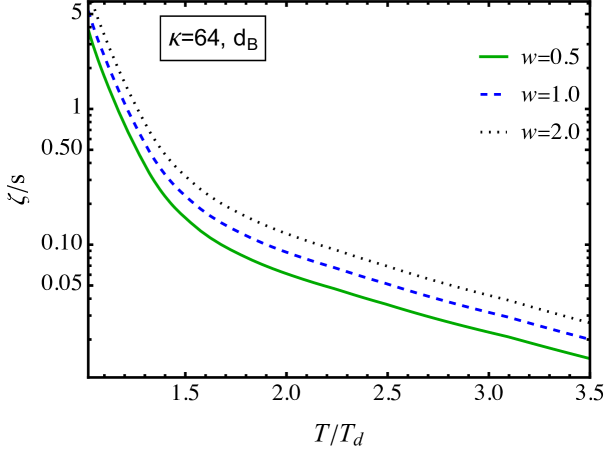
In Fig. 15, we show the ratio of the bulk viscosity to the entropy, versus temperature, for the two ansatzes, $d_{A}$ and $d_{B}$. We choose the parameters to fix the coefficients in the logarithms as $w=1$ and $\kappa=64$. We compare our result with the Gribov-Zwanziger model of Ref. [70], and find that our result for $\zeta/s$ is much larger, almost an order of magnitude. The value of $\zeta/s$ is $\sim 1.59$ and $1.71$ for $d_{A}$ and $d_{B}$.

The dependencies of the parameters $\kappa$ and $w$ on $\zeta/s$ are shown in Fig. 16. The left panel of Fig. 16 demonstrates a large sensitivity to the value of the parameter $\kappa$, which is greatest as $T\rightarrow T_{d}$. Similar to the parameter $\kappa$, there is a large uncertainty on $w$, especially as $T\rightarrow T_{d}$, although it is weaker than for $\kappa$.

Figure 16: Left: Ratio of the bulk viscosity to the entropy density for different parameter sets of $\kappa$. Right: Ratio of the bulk viscosity to the entropy density for different parameter sets of $w$.

The ratio of bulk viscosity $\zeta$ to shear viscosity $\eta$ has a thermodynamic significance as it reflects the type of dissipative response a medium exhibits in nonequilibrium conditions, particularly near phase transitions.

Figure 17: Left: Ratio of the bulk viscosity to the shear viscosity with the ansatz of Eq. (28). Right: Ratio of the bulk viscosity to the shear viscosity scaled with the square of the conformality measure ($\Delta v_{s}^{2}$).

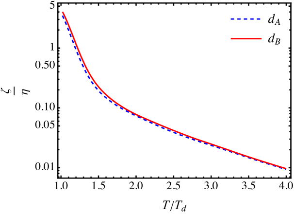
Bulk viscosity, which relates to the resistance to volume changes, tends to increase near phase transitions due to critical slowing down, where the medium struggles to equilibrate under isotropic stress. This increase is tied to the medium’s equation of state (EoS), which defines pressure and density relationships that influence the system’s relaxation toward equilibrium. Hence, the ratio $\zeta/\eta$ has an important physical significance.

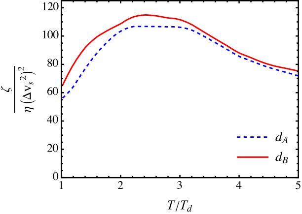
The left panel of Fig. 17  suggests a trend where the ratio decreases with increasing temperature. For $T/T_{d}$ values from around 1.5 to 3.5, $\zeta/\eta$ moves from values closer to 1 to significantly lower values. Lastly, the right panel of Fig. 17 shows the temperature dependence of the ratio of the bulk viscosity to the shear viscosity scaled with the square of the conformality measure ($\Delta v_{s}^{2}$). We comment on the relationship to other models in Eqs. (197) and (198).

VII Summary

The computation of the shear and bulk viscosities in our matrix model is admittedly involved, so we conclude by summarizing our results, and comparing to those obtained with different methods.

In heavy ion collisions at RHIC and LHC energies, experimentally it is observed that a nearly ideal hydrodynamics works amazingly well [71, 72, 73, 74, 75]. The standard paradigm for understanding this is the AdS/CFT correspondence: for a ${\cal N}=4$ $SU(N_{c})$ gauge theory at $N_{c}=\infty$ and $g^{2}N_{c}=\infty$  [76, 77, 78],

$$\left.\frac{\eta}{s}\right|^{\rm AdS/CFT}=\frac{1}{4\pi}\;\;,\;\;\left.\frac{\zeta}{s}\right|^{\rm AdS/CFT}=0\;.$$ (193)

As a conformally invariant theory, the dimensionless ratio $\eta/s$ is independent of temperature, and the bulk viscosity vanishes identically.

While our understanding of thermodynamics in equilibrium rests upon computations in lattice QCD, measuring transport coefficients is extraordinarily difficult. From the Kubo formula, they depend upon the relevant spectral densities as the frequency $\omega\rightarrow 0$. However, this requires analytic continuation from discrete, Euclidean $p_{0}$, to the continuous, Minkowski $\omega$. The most recent results from the lattice are from Ref. [79]; at $1.5\,T_{d}$,

$$\left.\frac{\eta}{s}\right|^{\text{Ref.\,\footnotesize{\cite[cite]{[\@@bibref{Number}{Altenkort:2022yhb}{}{}]}}}}_{1.5T_{d}}\approx 0.15-0.48\;\;;\;\;\left.\frac{\zeta}{s}\right|^{\text{ Ref.\,\footnotesize{\cite[cite]{[\@@bibref{Number}{Altenkort:2022yhb}{}{}]}}}}_{\rm 1.5T_{d}}\approx 0.017-0.059\;.$$ (194)

We can then compare results from AdS/CFT, Eq. (193), and the lattice, Eq. (194), to the results at leading logarithmic order in matrix models. For the shear viscosity, $\eta/s$, see Figs. 11, 12, 13, and 14; for the bulk viscosity, $\zeta/s$, see Figs. 15 and 16.

In a matrix model, the results are rather insensitive to which ansatz we use for the eigenvalue density, A or B in Eq. (28). They also depend upon the parameter $w$, which determines the running of the coupling, Eq. (165), and the constant $\kappa$, which fixes the behavior beyond leading logarithmic order in the coupling, Eq. (138). Using what we take as the optimal values of $w=0.5$ and $\kappa=64$, at $1.5\,T_{d}$ we find

$$\left.\frac{\eta}{s}\right|^{{\rm Fig.}\,\ref{fig:shear_viscosity_1}}_{1.5T_{d}}\approx 0.38-0.4\;;\;\left.\frac{\zeta}{s}\right|^{{\rm Fig.}\,\ref{fig:bulk_viscosity}}_{1.5T_{d}}\approx 0.076-0.087\;.$$ (195)

The value for $\eta/s$ at $1.5\,T_{d}$ is consistent with Ref. [79], although at the high end, while the bulk viscosity is somewhat larger than that of Ref. [79]. The matrix model, however, also provides results for the temperature dependence of each quantity.

If the coupling constant runs relatively slowly with temperature, as is true for the moderate values of the coupling constant which we use, then as the temperature $T\rightarrow T_{d}$, the principle way by which $\eta/s$ decreases is if the expectation value(s) of the Polyakov loops decrease as well. In the pure glue theory, for three colors the decrease in the expectation value of the first Polyakov loop is not very large, though: from $\langle\ell_{1}\rangle\rightarrow 1.0$ as $T\rightarrow\infty$ to $\langle\ell_{1}\rangle\approx 0.4$ at the deconfining transition $T_{d}$; for $N_{c}=\infty$, $\langle\ell_{1}\rangle\approx 0.5$ at $T_{d}$. Thus at $T_{d}$, the decrease in the shear viscosity is relatively moderate, as illustrated in Fig. 11. The precise temperature dependence is sensitive to varying $\kappa$, Fig. 12, or $w$, Fig. 13. These changes tend to bring $\eta/s$ much closer to the perturbative value.

In contrast, for the bulk viscosity, $\zeta/s$ increases sharply from $1.5T_{d}$ to $T_{d}$. From Fig. 15, with $w=0.5$ and $\kappa=64$, at the transition temperature the bulk viscosity is large,

$$\left.\frac{\zeta}{s}\right|^{{\rm Fig.}\,\footnotesize{\ref{fig:bulk_viscosity}}}_{T_{d}}\approx 1.6-1.7\;.$$ (196)

The variation with respect to $\kappa$ and $w$ are shown in Fig. 16. Varying $\kappa$, at $T_{d}$ we find that $\zeta/s\approx 1.1-4$; varying $w$, at $T_{d}$ the matrix model gives $\zeta/s\approx 4-7$. The variation in these values and the sensitivity with respect to $w$ and $\kappa$, indicate the limitations of our model and the attendant assumptions. However, what is clear is that $\zeta/s$ increases strongly as $T\rightarrow T_{d}$.

It is also useful to compare our results with those obtained in other effective models. Corrections to the perturbative results for the shear and bulk viscosity were estimated in Refs. [80, 81, 82, 83]. Higher order corrections do tend to decrease $\eta/s$.

Another approach is to use a quasiparticle model, where the gluon masses are $m_{\rm gl}\sim g(T)T$. Taking $g(T)$ to increase strongly as $T\rightarrow T_{d}$, a small pressure is obtained by letting $g(T)$ become large as $T\rightarrow T_{d}$, so the gluon quasiparticles are (very) heavy. This was done in Refs. [84, 85], with results that depend strongly on temperature. As $T$ decreases, it reaches a minimum at $T_{\rm min}\approx 1.1\,T_{d}$, and then increases sharply. The shear viscosity is very small at $T_{\rm min}$, with $\eta/s(T_{\rm min})\approx 0.1$, close to the AdS/CFT bound. For the bulk viscosity, it is extremely small until $\approx 1.2\,T_{d}$, where it then increases sharply, and is large, $\zeta/s\approx 0.25$ at $T_{\rm min}$. In contrast to our model, $\eta/s$ is much smaller at $T_{\rm min}$, while our values for $\zeta/s\approx 0.76-0.81$ at $1.1T_{d}$ (see Fig. 15) is larger than the quasiparticle model. Still, given the assumptions in both the quasiparticle model, and our matrix model, the results are not that far apart.

There are also results for the bulk viscosity from other models. For the bulk viscosity, in ${\cal N}^{*}=2$ SUSY gauge theories Buchel [86] established the bound

$$\frac{\zeta}{\eta}\times\frac{1}{(1/3-v_{s}^{2})}\geq 2\;.$$ (197)

However, this bound is not exact [87, 88, 89, 90].

Bounds on the bulk viscosity were also obtained by Dusling and Schaefer in Ref. [91]. In the relaxation time approximation to kinetic theory,

$$\frac{\zeta}{\eta}\times\frac{1}{(1/3-v_{s}^{2})^{2}}\approx 15\;.$$ (198)

This is stronger than the bound from ${\cal N}^{*}=2$ SUSY, in that, it involves the square of the difference in the speed of sound from the conformal limit, where $v_{s}^{2}=1/3$.

In the right panel of Fig. 17 we plot the same quantity as on the left-hand side of Eq. (198), $\zeta/\eta$ times $1/(1/3-v_{s}^{2})^{2}$. Unlike the relaxation time approximation, unsurprisingly, this is temperature dependent, with a value $\approx 56-65$ at $T_{d}$. The ratio then increases to a maximum of $\approx 105-114$ at $\approx 2.5T_{d}$, and then it falls off as $T$ increases further. In this ratio, there is sensitivity to which ansatz is used.

Still, the right panel of Fig. 17 shows that the relaxation time approximation gives a good rule of thumb, although the matrix model value is about five time larger, with a non-trivial dependence upon temperature.

There are other models to which we can compare. Using a Gribov-Zwanziger model, Refs. [92, 70, 93] find that $\zeta/s\approx 0.2$ at $T_{d}$. While large, ours is approximately an order of magnitude larger, $\zeta/s\approx 1.7$ at $T_{d}$.

There are also results from holographic models [94]. Anisotropic holographic models find that while the transverse shear viscosity obeys the AdS/CFT bound, that longitudinal to the direction of the anisotropy can be smaller than the bound [90]. Reference [95] also finds that in holographic models, $\eta/s$ can be below the AdS/CFT bound. Reference [96] finds $\eta/s$ has a minimum at $T_{d}$, with a model dependent value above $1/(4\pi)$. Reference [97] construct a model where $\eta/s$ is below the AdS/CFT bound, while $\zeta/s\approx 0.12$ at $T_{d}$. Reference [98] constructs a bottom-up model where $\eta/s$ is constant, equal to the AdS/CFT bound, with a small bulk viscosity, $\zeta/s\approx 0.045$ at $T_{d}$. Reference [99] found a large value for the bulk viscosity at the transition, $\zeta(T)/T^{3}\approx 0.1$ at $T_{d}$. Reference [100] finds a violation of the Buchel bound [86], in a model-dependent fashion. Reference [101] find $\zeta/s\approx 0.2$ at $T_{d}$. At $T_{d}$, Ref. [102] find a small minimum for the shear viscosity, $\eta/s\approx 0.2$, and for the bulk viscosity, $\zeta/s\approx 0.12$.

In all, at $T_{d}$ holographic models give a value of $\eta/s$ near the AdS/CFT bound, while $\zeta/s$ is larger than that from the lattice, but much smaller than in a matrix model.

Of course, what is relevant to QCD, and real experiments, is the theory with dynamical quarks. In a matrix model, the results for $\eta/s$ at the chiral phase transition, $T_{\chi}$ will certainly be much smaller than in the pure glue theory. This is because while the (first) Polyakov loop is relatively large at $T_{d}$, at the chiral phase transition, at $T_{\chi}$, the expectation value of the (first) Polyakov loop is rather small, $\langle\ell_{1}\rangle(T_{\chi})\approx 0.04$, Fig. 1 of Ref. [103]; see, also, Ref. [104]. This suggests that QCD enters a regime where, at $T_{\chi}$, chiral symmetry restoration occurs in a regime with nearly perfect confinement. In a matrix model, inexorably this will generate a much smaller value of $\eta/s$ [41]. The implications for the bulk viscosity are less clear, and can only be determined by computation, which is actively underway.

Appendix A Sign in the Boltzmann equation with teen ghosts

The sign of the Boltzmann equation with teen ghosts is a bit non-trivial. Here we explain how to obtain the sign in Eqs. (90) and (91). The point is that the teen ghost is equivalent to a fermion with periodic boundary conditions. In other words, it is equivalent to a fermion with an imaginary chemical potential $i\pi T$, which corresponds to the replacement of the fermion distribution function $f_{f}$ with $-f_{\text{\bngx 3}}$. This correspondence is more obvious in the case of equilibrium systems:

$$\frac{1}{\mathrm{e}^{(E_{p}-i(Q^{a}-Q^{b}+\pi T))/T}+1}=-\frac{1}{\mathrm{e}^{(E_{p}-i(Q^{a}-Q^{b}))/T}-1}=-f^{0}_{ab}\;.$$ (199)

From this correspondence, the sign of the left-hand side of the Boltzmann equation in Eq. (90) should be obvious. Let us see what happens to the sign of the collision term. In gluon-fermion scattering, we have a combination of distribution functions, $f_{\mathrm{g}}f_{f}(1+f_{\mathrm{g}})(1-f_{f})-(1+f_{\mathrm{g}})(1-f_{f})f_{\mathrm{g}}f_{f}$. This turns to

$$f_{\mathrm{g}}f_{f}(1+f_{\mathrm{g}})(1-f_{f})-(1+f_{\mathrm{g}})(1-f_{f})f_{\mathrm{g}}f_{f}$$

$$\to(-)\Bigl{[}f_{\mathrm{g}}f_{\text{\bngx 3}}(1+f_{\mathrm{g}})(1+f_{\text{\bngx 3}})-(1+f_{\mathrm{g}})(1+f_{\text{\bngx 3}})f_{\mathrm{g}}f_{\text{\bngx 3}}\Bigr{]}$$ (200)

in the gluon-teen scattering. We obtain the negative overall sign $(-)$. Similarly, for teen-teen scattering, we have

$$f_{f}f_{f}(1-f_{f})(1-f_{f})-(1-f_{f})(1-f_{f})f_{f}f_{f}$$

$$\to(+)\Bigl{[}f_{\text{\bngx 3}}f_{\text{\bngx 3}}(1+f_{\text{\bngx 3}})(1+f_{\text{\bngx 3}})-(1+f_{\text{\bngx 3}})(1+f_{\text{\bngx 3}})f_{\text{\bngx 3}}f_{\text{\bngx 3}}\Bigr{]}\,.$$ (201)

The sign is positive. These considerations show that the sign is determined by the evenness of the incoming ghost number, which corresponds to ${\mathcal{S}}_{\text{\bngx b}}\,{\mathcal{S}}_{\text{\bngx d}}$ in Eq. (91).

Appendix B Energy and pressure for teen particles

In kinetic theory, the energy-momentum tensor for teen ghost is given by

$$T^{\mu\nu}=-\int\frac{d\Omega}{4\pi}\int\frac{d^{3}p}{(2\pi)^{3}}\frac{p^{\mu}p^{\nu}}{E_{p}}\frac{1}{e^{\beta E_{p}}-1}\,.$$ (202)

Now,

$$T^{00} = -\int\frac{d\Omega}{4\pi}\int\frac{d^{3}p}{(2\pi)^{3}}\frac{p^{0}p^{0}}{E_{p}}\frac{1}{e^{\beta E_{p}}-1}\,,$$

$$\mathscr{E}^{\mathrm{kt}} \simeq -2\int_{0}^{\infty}\frac{dp_{\parallel}}{2\pi}\int\frac{p_{\perp}dp_{\perp}}{2\pi}|p_{\parallel}|\frac{1}{e^{\beta|p_{\parallel}|}-1}\,,$$

$$\mathscr{E}^{\mathrm{kt}} = -\frac{T^{2}T_{d}^{2}}{24}\,.$$ (203)

Take $\hat{n}\equiv\hat{z}$ and $p_{\perp}\sim T_{d}\ll p_{\parallel}$. The longitudinal pressure along the z-direction is

$$T^{33} = -\int\frac{d\Omega}{4\pi}\int\frac{d^{3}p}{(2\pi)^{3}}\frac{p^{3}p^{3}}{E_{p}}\frac{1}{e^{\beta E_{p}}-1}$$

$$\simeq -2\int_{0}^{\infty}\frac{dp_{\parallel}}{2\pi}\int\frac{p_{\perp}dp_{\perp}}{2\pi}|p_{\parallel}|\frac{1}{e^{\beta|p_{\parallel}|}-1}\,,$$

$$\mathscr{P}^{\mathrm{kt}}_{z} = -\frac{T^{2}T_{d}^{2}}{24}\,.$$ (204)

The perpendicular pressure is

$$T^{11}=T^{22} = -\int\frac{d\Omega}{4\pi}\int\frac{d^{3}p}{(2\pi)^{3}}\frac{p_{\perp}^{2}}{E_{p}}\frac{1}{e^{\beta E_{p}}-1}\,,$$

$$\mathscr{P}^{\mathrm{kt}}_{\perp} \simeq 0\,.$$ (205)

The difficulty is that in Eq. (204), one should average over the direction of the teen field, which gives $\mathscr{P}^{\mathrm{kt}}=-T^{2}T_{d}^{2}/72$, so that in kinetic theory, the teen field looks three dimensional, with $\mathscr{E}^{\mathrm{kt}}=3\mathscr{P}^{\mathrm{kt}}$. If we compute directly from thermodynamics, though, we obtain $\mathscr{P}^{\mathrm{th}}=\mathscr{E}^{\mathrm{th}}=-T^{2}T_{d}^{2}/24$, as expected for a two dimensional field.

Thus, as noted in Sec. (VI), kinetic theory gives the wrong pressure for a teen field. In computing the bulk viscosity, we avoided this by taking $\Delta v_{s}^{2}$ from thermodynamics. In turn this is fit to the lattice results, through the functions $d_{A}(T)$ and $d_{B}(T)$, Eq. 28.

We next discuss how to obtain a kinetic theory for teen particles which is consistent with a direct computation in thermodynamics. This considers the analogy to a magnetic field, where there is a difference between computing at constant magnetic field or constant flux.

We start with the energy density and pressure, defined from the partition function $\mathcal{Z}$, as

$$\mathscr{E}=-\frac{1}{V}\frac{\mathrm{~d}\log\mathcal{Z}}{\mathrm{~d}(1/T)}\,,\quad\quad\mathscr{P}_{i}=\frac{T}{V}L_{i}\frac{\mathrm{~d}\log\mathcal{Z}}{\mathrm{~d}L_{i}}\,,$$ (206)

where $L_{i}$ is the length of the system along i-th direction. The energy density in Eq. (206) becomes

$$\mathscr{E} = (2-1)T\int\frac{d\Omega_{n}}{4\pi}\int\frac{dp_{\|}}{2\pi}\int\frac{d^{2}p_{\perp}}{(2\pi)^{2}}\ln\left(1-e^{-\beta\left|p_{\|}\right|}\right)$$ (207)

$$= T\frac{1}{4\pi^{2}}\int_{0}^{T_{d}}dp_{\perp}p_{\perp}\int_{-\infty}^{\infty}dp_{\|}\ln\left(1-e^{-\beta\left|p_{\|}\right|}\right)$$

$$= -\frac{1}{24}T_{d}^{2}T^{2}\,.$$

Note that the energy density is the same, whether computed in kinetic theory, or from the partition function.

For the pressure $\mathscr{P}_{i}$, one can calculate the derivatives of the partition function in in two ways:

1. Keeping the energy density $\mathscr{E}$ constant, analogous to constant magnetic field $B$.

2. Keeping the longitudinal energy density $\mathscr{E}L_{x}L_{y}$ constant, which is analogous to constant magnetic flux $\Phi$.

In the first case, at constant $\mathscr{E}$, the pressure is

$$\mathscr{P}^{\mathrm{th}}_{i}=\frac{T}{V}\frac{\mathrm{~\partial}\log\mathcal{Z}}{\mathrm{\partial}\log L_{i}}=-\frac{1}{24}T_{d}^{2}T^{2}\,.$$ (208)

The second case, with constant longitudinal energy density, corresponds to the conventional energy momentum tensor, in which the pressure is given by Eqs. (204) and (205). To see this, note that

$$\mathscr{P}_{i}^{\mathrm{kt}} = \frac{T}{V}\frac{\partial\log\mathcal{Z}}{\partial\log L_{i}}+\left.\frac{T}{V}\frac{\partial\log\mathcal{Z}}{\partial\mathscr{E}}\cdot\frac{\partial\mathscr{E}}{\partial\log L_{i}}\right|_{\mathrm{kt}}=\mathscr{P}_{i}^{\mathrm{th}}+\left.\frac{T}{V}\frac{\partial\log\mathcal{Z}}{\partial\mathscr{E}}\cdot\frac{\partial\mathscr{E}}{\partial\log L_{i}}\right|_{\mathrm{kt}}\,.$$ (209)

Since $\mathscr{E}$ decreases with $L_{x}$ and $L_{y}$,

$$\mathscr{P}_{z}^{\mathrm{kt}} = \mathscr{P}_{z}^{\mathrm{th}}=-\frac{1}{24}T^{2}T_{d}^{2}\qquad\mbox{and}$$

$$\mathscr{P}_{\perp}^{\mathrm{kt}} = \mathscr{P}_{\perp}^{\mathrm{th}}+\frac{\partial\mathscr{P}_{\perp}^{\mathrm{th}}}{\partial\mathscr{E}}(-\mathscr{E})=\mathscr{P}_{\perp}^{\mathrm{th}}+(1)(-\mathscr{P}_{\perp}^{\mathrm{th}})=\mathscr{P}_{\perp}^{\mathrm{th}}-\mathscr{P}_{\perp}^{\mathrm{th}}=0\,.$$

Thus, the results from $T^{\mu\nu}$ and thermodynamics are consistent with each other, whether one computes at constant longitudinal energy density, or at constant energy density.

Appendix C Zero mode

The analysis of the collision kernel for the bulk viscosity, Eq. (191), involves zero modes that do not arrive for the shear viscosity. Since only $2\leftrightarrow 2$ scattering processes are considered, there are zero modes for the conservation of particle number. There are also zero modes for energy conservation. Because of this, finding the inverse of the $\bar{\mathcal{L}}$ matrix is ill-defined.

If only gluons scatter, in Eq. (191) only the term $\sim Y^{\mathrm{gg}}_{mn}$ contributes, and has zero modes. Reference [46] adds a term to lift this degeneracy and computes the inverse of $\bar{\mathcal{L}}$, proportional to a parameter $\lambda$. They then check, numerically, that the result is independent of $\lambda$.

Adding teen fields complicates the analysis, as teens contribute to a variety of processes. The scattering of gluons into themselves, $\mathrm{gg}\rightarrow\mathrm{gg}$, gives a term $\sim T^{6}Y^{\mathrm{gg}}_{mn}$; that from teens with themselves, $\text{\bngx 3}\text{\bngx 3}\rightarrow\text{\bngx 3}\text{\bngx 3}$, gives a term $T_{d}^{4}T^{2}Y^{\text{\bngx 3}\text{\bngx 3}}_{mn}$. These contributions have zero modes.

However, there are additional scattering from glue teen scattering, $\text{\bngx 3}\mathrm{g}\rightarrow\text{\bngx 3}\mathrm{g}$. For the glue-glue term in the upper left hand corner of Eq. (191), the total is $T^{6}\,{Y}^{\mathrm{gg}}_{mn}+T^{4}\,T_{d}^{2}{\overline{Y}}^{\mathrm{gg}}_{mn}$. Similarly, for the teen-teen term in the lower right hand corner, the total is $T_{d}^{4}\,T^{2}{Y}^{\text{\bngx 3}\text{\bngx 3}}_{mn}+T^{4}\,T_{d}^{2}{\overline{Y}}^{\text{\bngx 3}\text{\bngx 3}}_{mn}$. Because of the additional contributions, these terms no longer have zero modes.

However, there are also off-diagonal terms in Eq. (191). These are $T^{4}T_{d}^{2}Y^{\mathrm{g}\text{\bngx 3}}_{mn}$ and $T^{4}T_{d}^{2}Y^{\text{\bngx 3}\mathrm{g}}_{mn}$, and each has zero modes. By trial and error, we find that a term which lifts the degeneracy of the scattering kernel in Eq. (191) is

$$\bar{\Lambda}^{\text{\bngx b},\text{\bngx d}}_{mn}\rightarrow\bar{\Lambda}^{\text{\bngx b},\text{\bngx d}}_{mn}+(1-\delta^{\text{\bngx b},\text{\bngx d}})\;\frac{\lambda g^{4}N_{c}^{4}}{2(2\pi)^{5}}\;\log\left(\frac{\kappa}{g^{2}N_{c}}\right)\bigg{(}\int\frac{d^{3}p}{(2\pi)^{3}}p^{2}\frac{\partial\psi_{\text{\bngx b},m}}{\partial p}\bigg{)}\bigg{(}\int\frac{d^{3}k}{(2\pi)^{3}}k^{2}\frac{\partial\psi_{\text{\bngx d},m}}{\partial k}\bigg{)}\,.\ \ \hskip 14.22636pt$$ (210)

We checked numerically that for any positive $\lambda$, $T\sum_{\text{\bngx b}}\sum_{n=0}^{\infty}V_{n}^{\text{\bngx b}}\big{(}\bar{\mathcal{L}}^{-1}V\big{)}_{n}^{\text{\bngx b}}$ is independent of $\lambda$.

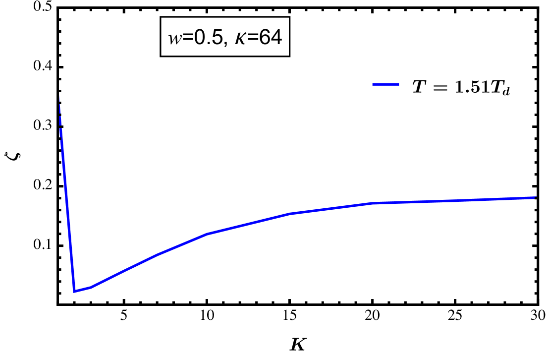
In Fig. 18 we illustrate the convergence of bulk viscosity versus $K$, the dimension of the basis functions, for one typical value of the temperature and other parameters. The convergence for other values was consistently similar. While $K$ is in principle infinite, in Ref. [46] they found good convergence for small values of $K\leq 5$. In contrast, we uniformly found convergence by values of $K\leq 20-30$.

Figure 18: Variation of bulk viscosity with increasing basis number at $T/T_{d}=1.51$, with $w=0.5$ and $\kappa=64$.

References

- Gross et al. [1981] D. J. Gross, R. D. Pisarski, and L. G. Yaffe, QCD and Instantons at Finite Temperature, Rev.Mod.Phys. 53, 43 (1981).
- Weiss [1981] N. Weiss, The Effective Potential for the Order Parameter of Gauge Theories at Finite Temperature, Phys. Rev. D 24, 475 (1981).
- Bhattacharya et al. [1991] T. Bhattacharya, A. Gocksch, C. P. Korthals Altes, and R. D. Pisarski, Interface tension in an SU(N) gauge theory at high temperature, Phys.Rev.Lett. 66, 998 (1991).
- Bhattacharya et al. [1992] T. Bhattacharya, A. Gocksch, C. Korthals Altes, and R. D. Pisarski, Z(N) interface tension in a hot SU(N) gauge theory, Nucl. Phys. B 383, 497 (1992), arXiv:hep-ph/9205231 .
- Gocksch and Pisarski [1993] A. Gocksch and R. D. Pisarski, Partition function for the eigenvalues of the Wilson line, Nucl. Phys. B 402, 657 (1993), arXiv:hep-ph/9302233 .
- Korthals Altes et al. [2000] C. P. Korthals Altes, R. D. Pisarski, and A. Sinkovics, The Potential for the phase of the Wilson line at nonzero quark density, Phys. Rev. D 61, 056007 (2000), arXiv:hep-ph/9904305 .
- Pisarski [2000] R. D. Pisarski, Quark gluon plasma as a condensate of SU(3) Wilson lines, Phys.Rev. D62, 111501 (2000), arXiv:hep-ph/0006205 [hep-ph] .
- Dumitru and Pisarski [2002] A. Dumitru and R. D. Pisarski, Two point functions for SU(3) Polyakov loops near T(c), Phys. Rev. D 66, 096003 (2002), arXiv:hep-ph/0204223 .
- Dumitru et al. [2004] A. Dumitru, Y. Hatta, J. Lenaghan, K. Orginos, and R. D. Pisarski, Deconfining phase transition as a matrix model of renormalized Polyakov loops, Phys. Rev. D 70, 034511 (2004), arXiv:hep-th/0311223 .
- Dumitru et al. [2005a] A. Dumitru, J. Lenaghan, and R. D. Pisarski, Deconfinement in matrix models about the Gross-Witten point, Phys. Rev. D 71, 074004 (2005a), arXiv:hep-ph/0410294 .
- Dumitru et al. [2005b] A. Dumitru, R. D. Pisarski, and D. Zschiesche, Dense quarks, and the fermion sign problem, in a SU(N) matrix model, Phys. Rev. D 72, 065008 (2005b), arXiv:hep-ph/0505256 .
- Oswald and Pisarski [2006] M. Oswald and R. D. Pisarski, Beta-functions for a SU(2) matrix model in 2 + epsilon dimensions, Phys. Rev. D 74, 045029 (2006), arXiv:hep-ph/0512245 .
- Pisarski [2006] R. D. Pisarski, Effective Theory of Wilson Lines and Deconfinement, Phys.Rev. D74, 121703 (2006), arXiv:hep-ph/0608242 [hep-ph] .
- Pisarski [1989] R. D. Pisarski, Scattering Amplitudes in Hot Gauge Theories, Phys. Rev. Lett. 63, 1129 (1989).
- Braaten and Pisarski [1990a] E. Braaten and R. D. Pisarski, Soft Amplitudes in Hot Gauge Theories: A General Analysis, Nucl. Phys. B 337, 569 (1990a).
- Braaten and Pisarski [1990b] E. Braaten and R. D. Pisarski, Resummation and Gauge Invariance of the Gluon Damping Rate in Hot QCD, Phys. Rev. Lett. 64, 1338 (1990b).
- Braaten and Pisarski [1990c] E. Braaten and R. D. Pisarski, Calculation of the gluon damping rate in hot QCD, Phys. Rev. D 42, 2156 (1990c).
- Braaten and Pisarski [1992] E. Braaten and R. D. Pisarski, Simple effective Lagrangian for hard thermal loops, Phys. Rev. D 45, R1827 (1992).
- Kelly et al. [1994a] P. F. Kelly, Q. Liu, C. Lucchesi, and C. Manuel, Deriving the hard thermal loops of QCD from classical transport theory, Phys. Rev. Lett. 72, 3461 (1994a), arXiv:hep-ph/9403403 .
- Kelly et al. [1994b] P. F. Kelly, Q. Liu, C. Lucchesi, and C. Manuel, Classical transport theory and hard thermal loops in the quark - gluon plasma, Phys. Rev. D 50, 4209 (1994b), arXiv:hep-ph/9406285 .
- Blaizot and Iancu [2002] J.-P. Blaizot and E. Iancu, The Quark gluon plasma: Collective dynamics and hard thermal loops, Phys. Rept. 359, 355 (2002), arXiv:hep-ph/0101103 .
- Bellac [2011] M. L. Bellac, Thermal Field Theory, Cambridge Monographs on Mathematical Physics (Cambridge University Press, 2011).
- Haque et al. [2014] N. Haque, A. Bandyopadhyay, J. O. Andersen, M. G. Mustafa, M. Strickland, and N. Su, Three-loop HTLpt thermodynamics at finite temperature and chemical potential, JHEP 05, 027, arXiv:1402.6907 [hep-ph] .
- Haque and Mustafa [2025] N. Haque and M. G. Mustafa, Hard Thermal Loop—Theory and applications, Prog. Part. Nucl. Phys. 140, 104136 (2025), arXiv:2404.08734 [hep-ph] .
- Hidaka and Pisarski [2008] Y. Hidaka and R. D. Pisarski, Suppression of the Shear Viscosity in a ”semi” Quark Gluon Plasma, Phys. Rev. D 78, 071501 (2008), arXiv:0803.0453 [hep-ph] .
- Hidaka and Pisarski [2010] Y. Hidaka and R. D. Pisarski, Small shear viscosity in the semi quark gluon plasma, Phys. Rev. D 81, 076002 (2010), arXiv:0912.0940 [hep-ph] .
- Hidaka and Pisarski [2009a] Y. Hidaka and R. D. Pisarski, Hard thermal loops, to quadratic order, in the background of a spatial ’t Hooft loop, Phys. Rev. D 80, 036004 (2009a), [Erratum: Phys.Rev.D 102, 059902 (2020)], arXiv:0906.1751 [hep-ph] .
- Hidaka and Pisarski [2009b] Y. Hidaka and R. D. Pisarski, Zero Point Energy of Renormalized Wilson Loops, Phys. Rev. D 80, 074504 (2009b), arXiv:0907.4609 [hep-ph] .
- Dumitru et al. [2011] A. Dumitru, Y. Guo, Y. Hidaka, C. P. K. Altes, and R. D. Pisarski, How Wide is the Transition to Deconfinement?, Phys. Rev. D 83, 034022 (2011), arXiv:1011.3820 [hep-ph] .
- Dumitru et al. [2012] A. Dumitru, Y. Guo, Y. Hidaka, C. P. K. Altes, and R. D. Pisarski, Effective Matrix Model for Deconfinement in Pure Gauge Theories, Phys. Rev. D 86, 105017 (2012), arXiv:1205.0137 [hep-ph] .
- Kashiwa et al. [2012] K. Kashiwa, R. D. Pisarski, and V. V. Skokov, Critical endpoint for deconfinement in matrix and other effective models, Phys.Rev. D85, 114029o (2012), arXiv:1205.0545 [hep-ph] .
- Pisarski and Skokov [2012] R. D. Pisarski and V. V. Skokov, Gross-Witten-Wadia transition in a matrix model of deconfinement, Phys. Rev. D 86, 081701 (2012), arXiv:1206.1329 [hep-th] .
- Bicudo et al. [2013] P. Bicudo, R. D. Pisarski, and E. Seel, Matrix model for deconfinement in a SU(2) gauge theory in 2+1 dimensions, Phys. Rev. D 88, 034007 (2013), arXiv:1306.2943 [hep-ph] .
- Kashiwa and Pisarski [2013] K. Kashiwa and R. D. Pisarski, Roberge-Weiss transition and ’t Hooft loops, Phys. Rev. D 87, 096009 (2013), arXiv:1301.5344 [hep-ph] .
- Lin et al. [2014] S. Lin, R. D. Pisarski, and V. V. Skokov, Collisional energy loss above the critical temperature in QCD, Phys. Lett. B 730, 236 (2014), arXiv:1312.3340 [hep-ph] .
- Lin et al. [2013] S. Lin, R. D. Pisarski, and V. V. Skokov, Zero interface tension at the deconfining phase transition for a matrix model of a gauge theory, Phys. Rev. D 87, 105002 (2013), arXiv:1301.7432 [hep-ph] .
- Smith et al. [2013] D. Smith, A. Dumitru, R. Pisarski, and L. von Smekal, Effective potential for SU(2) Polyakov loops and Wilson loop eigenvalues, Phys. Rev. D 88, 054020 (2013), arXiv:1307.6339 [hep-lat] .
- Bicudo et al. [2014] P. Bicudo, R. D. Pisarski, and E. Seel, Matrix model for deconfinement in a SU(Nc) gauge theory in 2+1 dimensions, Phys. Rev. D 89, 085020 (2014), arXiv:1402.5137 [hep-ph] .
- Gale et al. [2015] C. Gale, Y. Hidaka, S. Jeon, S. Lin, J.-F. Paquet, R. D. Pisarski, D. Satow, V. V. Skokov, and G. Vujanovic, Production and Elliptic Flow of Dileptons and Photons in a Matrix Model of the Quark-Gluon Plasma, Phys. Rev. Lett. 114, 072301 (2015), arXiv:1409.4778 [hep-ph] .
- Hidaka et al. [2015] Y. Hidaka, S. Lin, R. D. Pisarski, and D. Satow, Dilepton and photon production in the presence of a nontrivial Polyakov loop, JHEP 10, 005, arXiv:1504.01770 [hep-ph] .
- Pisarski and Skokov [2016] R. D. Pisarski and V. V. Skokov, Chiral matrix model of the semi-QGP in QCD, Phys. Rev. D 94, 034015 (2016), arXiv:1604.00022 [hep-ph] .
- Korthals Altes et al. [2020a] C. P. Korthals Altes, H. Nishimura, R. D. Pisarski, and V. V. Skokov, Free energy of a Holonomous Plasma, Phys. Rev. D 101, 094025 (2020a), arXiv:2002.00968 [hep-ph] .
- Hidaka and Pisarski [2021] Y. Hidaka and R. D. Pisarski, Effective models of a semi-quark-gluon plasma, Phys. Rev. D 104, 074036 (2021), arXiv:2009.03903 [hep-ph] .
- Arnold et al. [2000] P. B. Arnold, G. D. Moore, and L. G. Yaffe, Transport coefficients in high temperature gauge theories. 1. Leading log results, JHEP 11, 001, arXiv:hep-ph/0010177 .
- Arnold et al. [2003] P. B. Arnold, G. D. Moore, and L. G. Yaffe, Transport coefficients in high temperature gauge theories. 2. Beyond leading log, JHEP 05, 051, arXiv:hep-ph/0302165 .
- Arnold et al. [2006] P. B. Arnold, C. Dogan, and G. D. Moore, The Bulk Viscosity of High-Temperature QCD, Phys. Rev. D 74, 085021 (2006), arXiv:hep-ph/0608012 .
- Nishimura et al. [2018] H. Nishimura, R. D. Pisarski, and V. V. Skokov, Finite-temperature phase transitions of third and higher order in gauge theories at large , Phys. Rev. D97, 036014 (2018), arXiv:1712.04465 [hep-th] .
- Korthals Altes et al. [2020b] C. P. Korthals Altes, H. Nishimura, R. D. Pisarski, and V. V. Skokov, Conundrum for the free energy of a holonomous gluonic plasma at cubic order, Phys. Lett. B 803, 135336 (2020b), arXiv:1911.10209 [hep-th] .
- Gaiotto et al. [2015] D. Gaiotto, A. Kapustin, N. Seiberg, and B. Willett, Generalized Global Symmetries, JHEP 02, 172, arXiv:1412.5148 [hep-th] .
- Gupta et al. [2008] S. Gupta, K. Huebner, and O. Kaczmarek, Renormalized Polyakov loops in many representations, Phys. Rev. D 77, 034503 (2008), arXiv:0711.2251 [hep-lat] .
- Fukushima [2004] K. Fukushima, Chiral effective model with the Polyakov loop, Phys. Lett. B 591, 277 (2004), arXiv:hep-ph/0310121 .
- Korthals-Altes et al. [1999] C. Korthals-Altes, A. Kovner, and M. A. Stephanov, Spatial ’t Hooft loop, hot QCD and Z(N) domain walls, Phys. Lett. B 469, 205 (1999), arXiv:hep-ph/9909516 .
- Mykkanen et al. [2012] A. Mykkanen, M. Panero, and K. Rummukainen, Casimir scaling and renormalization of Polyakov loops in large-N gauge theories, JHEP 05, 069, arXiv:1202.2762 [hep-lat] .
- Caselle et al. [2018] M. Caselle, A. Nada, and M. Panero, QCD thermodynamics from lattice calculations with nonequilibrium methods: The SU(3) equation of state, Phys. Rev. D 98, 054513 (2018), arXiv:1801.03110 [hep-lat] .
- Datta and Gupta [2010] S. Datta and S. Gupta, Continuum Thermodynamics of the Gluo Plasma, Phys.Rev. D82, 114505 (2010), arXiv:1006.0938 [hep-lat] .
- Giusti et al. [2025] L. Giusti, M. Hirasawa, M. Pepe, and L. Virzì, A precise study of the SU(3) Yang-Mills theory across the deconfinement transition, (2025), arXiv:2501.10284 [hep-lat] .
- Moore and Saremi [2008] G. D. Moore and O. Saremi, Bulk viscosity and spectral functions in QCD, JHEP 09, 015, arXiv:0805.4201 [hep-ph] .
- Jackson and Peshier [2018] G. Jackson and A. Peshier, Re-running the QCD shear viscosity, J. Phys. G 45, 095001 (2018), arXiv:1711.02119 [hep-ph] .
- Ghiglieri et al. [2018] J. Ghiglieri, G. D. Moore, and D. Teaney, QCD Shear Viscosity at (almost) NLO, JHEP 03, 179, arXiv:1802.09535 [hep-ph] .
- Moore [2020] G. D. Moore, Shear viscosity in QCD and why it’s hard to calculate, in Criticality in QCD and the Hadron Resonance Gas (2020) arXiv:2010.15704 [hep-ph] .
- Danhoni and Moore [2023] I. Danhoni and G. D. Moore, Hot and dense QCD shear viscosity at leading log, JHEP 02, 124, arXiv:2212.02325 [hep-ph] .
- Danhoni and Moore [2024] I. Danhoni and G. D. Moore, Hot and dense QCD shear viscosity at (almost) NLO, JHEP 09, 075, arXiv:2408.00524 [hep-ph] .
- MacKay [2024] N. M. MacKay, Shear Viscosity of Collider-Produced QCD Matter I: AMY Formalism vs. A Modified Relaxation Time Approximation in 0-flavor SU(3) Theory, (2024), arXiv:2407.16856 [nucl-th] .
- Arnold and Zhai [1994] P. B. Arnold and C.-X. Zhai, The Three loop free energy for pure gauge QCD, Phys. Rev. D50, 7603 (1994), arXiv:hep-ph/9408276 [hep-ph] .
- Arnold and Yaffe [1995] P. B. Arnold and L. G. Yaffe, The NonAbelian Debye screening length beyond leading order, Phys. Rev. D 52, 7208 (1995), arXiv:hep-ph/9508280 .
- Baym et al. [1990] G. Baym, H. Monien, C. J. Pethick, and D. G. Ravenhall, Transverse Interactions and Transport in Relativistic Quark - Gluon and Electromagnetic Plasmas, Phys. Rev. Lett. 64, 1867 (1990).
- Fukushima and Su [2013] K. Fukushima and N. Su, Stabilizing perturbative Yang-Mills thermodynamics with Gribov quantization, Phys. Rev. D 88, 076008 (2013), arXiv:1304.8004 [hep-ph] .
- Madni et al. [2023] S. Madni, A. Mukherjee, A. Bandyopadhyay, and N. Haque, Estimation of the diffusion coefficient of heavy quarks in light of Gribov-Zwanziger action, Phys. Lett. B 838, 137714 (2023), arXiv:2210.03076 [hep-ph] .
- Kovtun et al. [2003] P. Kovtun, D. T. Son, and A. O. Starinets, Holography and hydrodynamics: Diffusion on stretched horizons, JHEP 10, 064, arXiv:hep-th/0309213 .
- Jaiswal and Haque [2020] A. Jaiswal and N. Haque, Covariant kinetic theory and transport coefficients for Gribov plasma, Phys. Lett. B 811, 135936 (2020), arXiv:2005.01303 [hep-ph] .
- Luzum and Romatschke [2008] M. Luzum and P. Romatschke, Conformal Relativistic Viscous Hydrodynamics: Applications to RHIC results at s(NN)**(1/2) = 200-GeV, Phys. Rev. C 78, 034915 (2008), [Erratum: Phys.Rev.C 79, 039903 (2009)], arXiv:0804.4015 [nucl-th] .
- Casalderrey-Solana et al. [2014] J. Casalderrey-Solana, H. Liu, D. Mateos, K. Rajagopal, and U. A. Wiedemann, Gauge/String Duality, Hot QCD and Heavy Ion Collisions (Cambridge University Press, 2014) arXiv:1101.0618 [hep-th] .
- Gale et al. [2013] C. Gale, S. Jeon, and B. Schenke, Hydrodynamic Modeling of Heavy-Ion Collisions, Int. J. Mod. Phys. A 28, 1340011 (2013), arXiv:1301.5893 [nucl-th] .
- Romatschke and Romatschke [2019] P. Romatschke and U. Romatschke, Relativistic Fluid Dynamics In and Out of Equilibrium, Cambridge Monographs on Mathematical Physics (Cambridge University Press, 2019) arXiv:1712.05815 [nucl-th] .
- Nagle and Zajc [2018] J. L. Nagle and W. A. Zajc, Small System Collectivity in Relativistic Hadronic and Nuclear Collisions, Ann. Rev. Nucl. Part. Sci. 68, 211 (2018), arXiv:1801.03477 [nucl-ex] .
- Policastro et al. [2001] G. Policastro, D. T. Son, and A. O. Starinets, The Shear viscosity of strongly coupled N=4 supersymmetric Yang-Mills plasma, Phys. Rev. Lett. 87, 081601 (2001), arXiv:hep-th/0104066 .
- Kovtun et al. [2005] P. Kovtun, D. T. Son, and A. O. Starinets, Viscosity in strongly interacting quantum field theories from black hole physics, Phys. Rev. Lett. 94, 111601 (2005), arXiv:hep-th/0405231 .
- Son and Starinets [2007] D. T. Son and A. O. Starinets, Viscosity, Black Holes, and Quantum Field Theory, Ann. Rev. Nucl. Part. Sci. 57, 95 (2007), arXiv:0704.0240 [hep-th] .
- Altenkort et al. [2023] L. Altenkort, A. M. Eller, A. Francis, O. Kaczmarek, L. Mazur, G. D. Moore, and H.-T. Shu, Viscosity of pure-glue QCD from the lattice, Phys. Rev. D 108, 014503 (2023), arXiv:2211.08230 [hep-lat] .
- Xu et al. [2008] Z. Xu, C. Greiner, and H. Stocker, PQCD calculations of elliptic flow and shear viscosity at RHIC, Phys. Rev. Lett. 101, 082302 (2008), arXiv:0711.0961 [nucl-th] .
- Carrington and Kovalchuk [2009] M. E. Carrington and E. Kovalchuk, Leading order QCD shear viscosity from the three-particle irreducible effective action, Phys. Rev. D 80, 085013 (2009), arXiv:0906.1140 [hep-ph] .
- Chen et al. [2010] J.-W. Chen, H. Dong, K. Ohnishi, and Q. Wang, Shear Viscosity of a Gluon Plasma in Perturbative QCD, Phys. Lett. B 685, 277 (2010), arXiv:0907.2486 [nucl-th] .
- Chen et al. [2013] J.-W. Chen, J. Deng, H. Dong, and Q. Wang, Shear and bulk viscosities of a gluon plasma in perturbative QCD: Comparison of different treatments for the ggggg process, Phys. Rev. C 87, 024910 (2013), arXiv:1107.0522 [hep-ph] .
- Bluhm et al. [2009] M. Bluhm, B. Kampfer, and K. Redlich, Viscosities in the Gluon-Plasma within a Quasiparticle Model, Nucl. Phys. A 830, 737C (2009), arXiv:0907.3841 [hep-ph] .
- Bluhm et al. [2011] M. Bluhm, B. Kampfer, and K. Redlich, Bulk and shear viscosities of the gluon plasma in a quasiparticle description, Phys. Rev. C 84, 025201 (2011), arXiv:1011.5634 [hep-ph] .
- Buchel [2008] A. Buchel, Bulk viscosity of gauge theory plasma at strong coupling, Phys. Lett. B 663, 286 (2008), arXiv:0708.3459 [hep-th] .
- Yarom [2010] A. Yarom, Notes on the bulk viscosity of holographic gauge theory plasmas, JHEP 04, 024, arXiv:0912.2100 [hep-th] .
- Buchel [2012] A. Buchel, Violation of the holographic bulk viscosity bound, Phys. Rev. D 85, 066004 (2012), arXiv:1110.0063 [hep-th] .
- Buchel et al. [2011] A. Buchel, U. Gursoy, and E. Kiritsis, Holographic bulk viscosity: GPR versus EO, JHEP 09, 095, arXiv:1104.2058 [hep-th] .
- Rebhan and Steineder [2012] A. Rebhan and D. Steineder, Violation of the Holographic Viscosity Bound in a Strongly Coupled Anisotropic Plasma, Phys. Rev. Lett. 108, 021601 (2012), arXiv:1110.6825 [hep-th] .
- Dusling and Schäfer [2012] K. Dusling and T. Schäfer, Bulk viscosity, particle spectra and flow in heavy-ion collisions, Phys. Rev. C 85, 044909 (2012), arXiv:1109.5181 [hep-ph] .
- Florkowski et al. [2016] W. Florkowski, R. Ryblewski, N. Su, and K. Tywoniuk, Bulk viscosity in a plasma of Gribov-Zwanziger gluons, Acta Phys. Polon. B 47, 1833 (2016), arXiv:1504.03176 [hep-ph] .
- Madni et al. [2024] S. Madni, A. Mukherjee, A. Jaiswal, and N. Haque, Shear and bulk viscosity of the quark-gluon plasma with Gribov gluons and quasiparticle quarks, Phys. Rev. D 110, 116035 (2024), arXiv:2401.08384 [hep-ph] .
- DeWolfe [2018] O. DeWolfe, TASI Lectures on Applications of Gauge/Gravity Duality, PoS TASI2017, 014 (2018), arXiv:1802.08267 [hep-th] .
- Mamo [2012] K. A. Mamo, Holographic RG flow of the shear viscosity to entropy density ratio in strongly coupled anisotropic plasma, JHEP 10, 070, arXiv:1205.1797 [hep-th] .
- Cremonini et al. [2012] S. Cremonini, U. Gursoy, and P. Szepietowski, On the Temperature Dependence of the Shear Viscosity and Holography, JHEP 08, 167, arXiv:1206.3581 [hep-th] .
- Li et al. [2015] D. Li, S. He, and M. Huang, Temperature dependent transport coefficients in a dynamical holographic QCD model, JHEP 06, 046, arXiv:1411.5332 [hep-ph] .
- Finazzo et al. [2015] S. I. Finazzo, R. Rougemont, H. Marrochio, and J. Noronha, Hydrodynamic transport coefficients for the non-conformal quark-gluon plasma from holography, JHEP 02, 051, arXiv:1412.2968 [hep-ph] .
- Yaresko and Kampfer [2014] R. Yaresko and B. Kampfer, Bulk viscosity of the gluon plasma in a holographic approach, Acta Phys. Polon. Supp. 7, 137 (2014), arXiv:1403.3581 [hep-ph] .
- Attems et al. [2016] M. Attems, J. Casalderrey-Solana, D. Mateos, I. Papadimitriou, D. Santos-Oliván, C. F. Sopuerta, M. Triana, and M. Zilhão, Thermodynamics, transport and relaxation in non-conformal theories, JHEP 10, 155, arXiv:1603.01254 [hep-th] .
- Mamo [2019] K. A. Mamo, Strongly coupled supersymmetric Yang-Mills plasma on the Coulomb branch. II. Transport coefficients and hard probe parameters, Phys. Rev. D 100, 066011 (2019), arXiv:1610.09793 [hep-th] .
- Ballon-Bayona et al. [2021] A. Ballon-Bayona, L. A. H. Mamani, A. S. Miranda, and V. T. Zanchin, Effective holographic models for QCD: Thermodynamics and viscosity coefficients, Phys. Rev. D 104, 046013 (2021), arXiv:2103.14188 [hep-th] .
- Petreczky and Schadler [2015] P. Petreczky and H. P. Schadler, Renormalization of the Polyakov loop with gradient flow, Phys. Rev. D 92, 094517 (2015), arXiv:1509.07874 [hep-lat] .
- Bazavov et al. [2016] A. Bazavov, N. Brambilla, H. T. Ding, P. Petreczky, H. P. Schadler, A. Vairo, and J. H. Weber, Polyakov loop in 2+1 flavor QCD from low to high temperatures, Phys. Rev. D 93, 114502 (2016), arXiv:1603.06637 [hep-lat] .