Induced Gravitational Waves as Cosmic Tracers of Leptogenesis

Abstract

We demonstrate that induced gravitational waves (IGWs) can naturally emerge within the framework of thermal leptogenesis models, thereby providing a robust probe for exploring this theory at remarkably high energy scales. To illustrate this principle, we put forth a basic leptogenesis model in which an early matter-dominated phase, tracing the leptogenesis scale, enhances the generation of gravitational waves induced by an early structure formation. Leveraging recent N-body and lattice simulation results for IGW computations in the non-linear regime, we show that it is possible to establish a direct link between the frequency and amplitude of these IGWs and the thermal leptogenesis scale.

Introduction.  Thermal leptogenesis is one of the most studied mechanisms for generating the Baryon Asymmetry of the Universe (BAU), owing to its simplicity and its direct link to low-energy neutrino physics [1, 2, 3]. While neutrino observables provide valuable insights into thermal leptogenesis given a proper treatment of the theory’s flavor structure [4, 5, 6, 7], a laboratory probe of the leptogenesis scale remains infeasible. This is because, in its simplest form, thermal leptogenesis occurs at extremely high temperatures, namely $T_{\text{lepto}}\sim M_{N}\gg\rm TeV$, where $M_{N}$ is the mass scale of the heavy right-handed neutrino (RHN), introduced on top of the Standard Model (SM) to generate light neutrino masses and facilitate BAU. Notably, we may probe such high energy scales with gravitational waves (GWs), thanks to the remarkable theoretical and experimental advancements in detecting the stochastic GW background [8, 9, 10, 11, 12, 13, 14, 15, 16, 17, 18]. As such, the LIGO-Virgo-KAGRA (LVK) collaboration has set upper bounds on the stochastic gravitational wave background at $\mathcal{O}(\text{Hz})$ frequencies [8]. Recent Pulsar Timing Array (PTA) observations indicate a nHz stochastic signal that may be of primordial origin [18]. Mid-frequency detectors like LISA, scheduled for launch in the 2030s, will feature a comprehensive physics pipeline [19].

In this Letter, we investigate the production of GWs in thermal leptogenesis models and argue that their frequency spectrum may encode information about the thermal leptogenesis scale. In particular, we focus on the induced gravitational waves (IGWs), sourced inevitably by primordial fluctuations in the very early universe due to second order gravitational interactions [20, 21, 22, 23, 24, 25, 26] (see Ref. [27] for a review). Interestingly enough, the presence of an early matter-dominated (eMD) epoch can intensify the production of IGWs [28, 26, 29, 30, 31, 32, 33, 34, 35, 36, 37, 27, 38, 39, 40, 41, 42, 43, 44, 45, 46, 47]. As we demonstrate here, simple leptogenesis models possess all the necessary prerequisites to achieve such an eMD era well-before Big Bang Nucleosynthesis (BBN), that is at $T_{\rm BBN}\gtrsim 4\,\text{MeV}$ [48, 49, 50, 51, 52], making IGWs a powerful probe of thermal leptogenesis.

Accurate estimations of the IGW spectrum generated during an eMD epoch are challenging; density fluctuations grow, and non-linear structures may emerge. Moreover, the specifics of transition to the following radiation-dominated era can impact the final IGW spectrum [33, 34]. One may restrict calculations to scales within the linear regime [32, 33, 34], where analytical or semi-analytical estimates are reliable. However, one expects a louder, more interesting GW signal in the non-linear regime [29, 30], though accurate predictions require numerical simulations [39, 44, 47]. Recently, Ref. [44] performed hybrid N-body and lattice simulations, following the formation and decay of early structures, and computed the resulting IGW spectrum.

Focusing in this work on the non-linear regime, we chart the parameter space of simple thermal leptogenesis models that yield a long enough eMD epoch with a detectable IGW signal. Furthermore, we argue that there is a concrete link between the leptogenesis scale and the IGW spectrum. Thus, a detection of an IGW background would hint at a particular leptogenesis scale. In any event, our work will serve to exclude a significant portion of our leptogenesis model parameter space.

Early matter-dominated epoch in thermal leptogenesis models.  We consider the widely studied ultraviolet realization of seesaw models based on the gauge $U(1)_{B-L}$ symmetry with coupling $g^{\prime}$, naturally embedded in many Grand Unified Theories (GUTs) [53, 54, 55]. The relevant terms of the Lagrangian read as

$$-\Delta\mathcal{L} \subset \frac{1}{2}y_{N}\overline{N_{R}}\Phi N_{R}^{C}+y_{D}\overline{N_{R}}\tilde{H}^{\dagger}L$$ (1)

$$+\frac{1}{4}\lambda_{H\Phi}H^{2}\Phi^{2}+V(\Phi,T)\,,$$

where the SM lepton doublets $L$, the SM Higgs doublet $H$, the right-handed neutrino fields $N_{R}$ and the scalar field $\Phi$ have $B-L$ charges -1, 0, -1 and 2, respectively. The first two terms are relevant for the masses of light and heavy neutrinos. After the $U(1)_{B-L}$ phase transition at a critical temperature $T_{c}$ (discussed later), $\Phi$ gets its vacuum expectation value $v_{\phi}$, and RHNs become massive. For simplicity, we assume a single RHN mass scale $M_{N}=y_{N}v_{\phi}$ with $v_{\Phi}=\mu/\sqrt{\lambda}$ determined from the zero-temperature potential $V(\Phi,0)=-\mu^{2}\Phi^{2}/2+\lambda\Phi^{4}/4$. These massive RHNs then decay CP-asymmetrically into lepton doublets and Higgs bosons, producing the lepton asymmetry around the temperature $T_{\rm lepto}\sim M_{N}$–owing to the chosen one-scale leptogenesis model, the final BAU needs to be computed within the resonant leptogenesis framework with quasi-degenerate RHNs [56]. Later on, once the SM Higgs takes its vacuum expectation value $v_{h}=174~{\rm GeV}$ at the electroweak phase transition, light neutrino masses $m_{\nu}\sim{y_{D}}^{2}v_{h}^{2}/M_{N}$ are generated via the type-I seesaw mechanism [57, 58, 59, 60]. The third term in Eq. (1) is the Higgs portal interaction, responsible for the decay $\Phi\to hh$, which may occur before or after the electroweak phase transition. Finally, the last term is the finite-temperature potential describing the $\Phi$ dynamics and the breaking of the $U(1)_{B-L}$ symmetry [61, 62, 63, 64, 65].

At very high temperatures, the $U(1)_{B-L}$ symmetry is unbroken and the potential has a minimum at $\Phi=0$. At lower temperatures, a secondary minimum is created at $\Phi\neq 0$, causing a potential barrier. The two minima become degenerate at the critical temperature $T_{c}$ and, for $T\lesssim T_{c}$, the barrier height decreases and disappears at $T_{*}$, making $\Phi=0$ into a maximum. The scalar field then transitions to $v_{\Phi}$. The transition strength is roughly characterized by the order parameter $\Phi_{c}/T_{c}$ with $\Phi_{c}=\Phi(T_{c})$ [63]. For $\Phi_{c}/T_{c}\ll 1$, the barrier vanishes quickly $(T_{c}\simeq T_{*}=2\sqrt{g^{\prime}}v_{\Phi})$, allowing for smooth rolling from $\Phi=0$ to $\Phi=v_{\Phi}$. We consider values of $\lambda$ and $g^{\prime}$ that satisfy this condition, specifically $\lambda\simeq{g^{\prime}}^{3}$ and $g^{\prime}\lesssim 10^{-1}$. This relation serves as a useful rule of thumb: increasing the power of $g^{\prime}$ raises the barrier height, hindering smooth rolling, while lowering it is disfavored by constraints discussed later. However, variations around $\lambda\sim{g^{\prime}}^{3}$ do not qualitatively alter the model, as the most sensitive parameter is the coupling $y_{N}$.

At temperatures $T<T_{*}$, the scalar field undergoes coherent oscillations around $v_{\Phi}$ with an angular frequency $m_{\Phi}=\sqrt{2\lambda}v_{\Phi}$, behaving like a non-relativistic matter component [66, 67]. If these oscillations persist due to a sufficiently long lifetime of the scalar filed, the Universe undergoes an eMD epoch which starts and ends at the temperatures $T_{\rm dom}$ and $T_{\rm dec}$, respectively. The former is given by $T_{\rm dom}=(\rho_{\Phi}(T_{c})/\rho_{R}(T_{c}))T_{c}$ with $\rho_{\Phi(R)}$ denoting the field (radiation) energy density, while the latter depends on the scalar field decay.

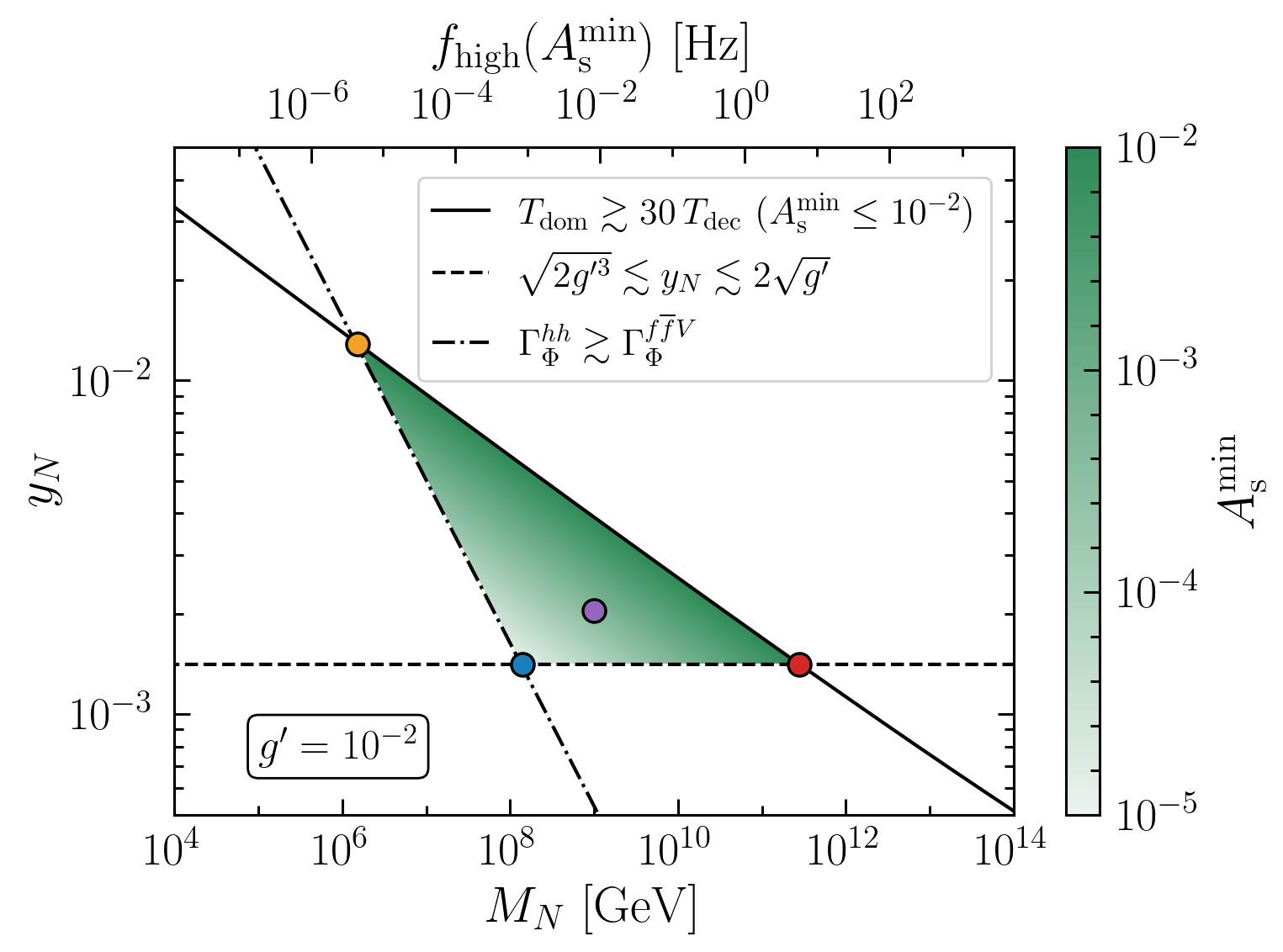
Figure 1: The green shaded region shows the parameter space linking the eMD epoch to the leptogenesis scale in the plane $M_{N}$-$y_{N}$ for $g^{\prime}=10^{-2}$. The black lines bound the allowed parameter space according to the constraints described in the main text. The color gradient displays the minimal value of the scalar amplitude required to produce IGWs (see Eq. (4)). The top x-axis reports the peak GW frequency $f_{\rm high}$ defined in Eq. (7) computed for $A_{\rm s}=A_{\rm s}^{\rm min}$. The points highlight the benchmark cases in Fig. 2.

In our scenario, the decay rate of $\Phi$ is governed by the Higgs portal coupling $\lambda_{H\Phi}\simeq\lambda_{H\Phi}^{\rm tree}+\lambda_{H\Phi}^{\text{1-loop}}$, which receives contributions from both tree-level and the inevitable one-loop effects. Note that $\lambda_{H\Phi}^{\text{1-loop}}$ is the minimal value of the Higgs portal coupling in seesaw models described by the first two terms in Eq. (1) [68, 69, 70]. Most interesting for our purposes is the case where $\lambda_{H\Phi}^{\text{1-loop}}>\lambda_{H\Phi}^{\rm tree}$ as it establishes a direct link between the leptogenesis scale (and so the neutrino parameters) and the lifetime of $\Phi$—thereby the IGW spectrum.

To ensure such a connection, we consider other decay channels negligible. The decays $\Phi\to Z^{\prime}Z^{\prime}$ and $\Phi\to NN$ are kinematically forbidden by requiring $M_{Z^{\prime}}=\sqrt{2}g^{\prime}v_{\Phi}>m_{\Phi}$ and $M_{N}\gtrsim m_{\Phi}$, respectively. The latter condition also rules out any off-shell, one-loop processes involving $N$ or $Z^{\prime}$ in the final state. Additionally, the one-loop $\Phi\Phi ZZ$ coupling, arising from the kinetic mixing [71, 72, 73, 74], is much weaker to produce any considerable effect. Another competitive channel in this model is the three-body decay to SM fermions and vector bosons, $\Phi\to f\bar{f}V$, mediated by virtual $Z^{\prime}$ at one-loop [75, 76].

In the limit $m_{\Phi}\gg m_{h}$, the one-loop $\Phi\to hh$ decay rate is given by [68, 69, 70, 77, 78]

$$\Gamma_{\Phi}^{hh}\simeq 1.8~{\rm MeV}~\frac{y_{N}^{3}}{\lambda^{1/2}}\left(\frac{M_{N}}{10^{11}~\text{GeV}}\right)^{3}~\ln^{2}\left(\frac{\Lambda_{\rm GUT}}{\Lambda}\right)\,,$$ (2)

where the logarithmic dependence accounts for the renormalization condition from the GUT scale, $\Lambda_{\rm GUT}\simeq 10^{16}~\text{GeV}$, to a lower scale $\Lambda$ [68, 69]. Note that while deriving Eq. (2), we use the seesaw relation $y_{D}=\sqrt{m_{\nu}M_{N}/v_{h}^{2}}$, with $m_{\nu}\simeq 0.01$ eV. This implies that the lifetime of $\Phi$ also depends on the light neutrino masses, making the model strongly connected to neutrino oscillation data and the upper bound $\sum m_{\nu}\lesssim 0.2~{\rm eV}$ [79, 80]. The decay temperature $T_{\text{dec}}$ can be determined by implicitly solving ${\rm H}(T_{\rm dec})\simeq\Gamma_{\Phi}^{hh}(T_{\rm dec})$, where ${\rm H}$ is the Hubble parameter and $\Lambda=T_{\rm dec}$.

In Fig. 1, we show without loss of generality the parameter space for $g^{\prime}=10^{-2}$ achieving an eMD era uniquely determined by the two remaining model parameters, i.e. the leptogenesis scale $M_{N}$ and the coupling $y_{N}$. We later discuss variations of $g^{\prime}$. Several necessary conditions tightly constrain the target parameter space.

First, the scalar field must dominate the Universe for long enough before decaying in order to develop non-linear structures. This requirement is related to the amplitude of the primordial spectrum of density fluctuations, say $A_{\rm s}$. Thus, given a duration of the eMD era, we may set a minium value for $A_{\rm s}$ (which we define as $A^{\rm min}_{\rm s}$ in Eq. (4)) and vice-versa. We take $A^{\rm min}_{\rm s}\leq 10^{-2}$ as a generous upper bound not to overproduce Primordial Black Holes (PBHs), see e.g. Refs. [81, 82, 83] and Ref. [84] for a general review.

Second, the coupling $y_{N}$ is bounded from below and above by demanding $m_{\Phi}\gtrsim M_{N}$ (prohibiting $\Phi\to NN$) and $T_{\rm lepto}\lesssim T_{c}$ (allowing the production of the lepton asymmetry), respectively. Laslty, the decay channel $\Phi\rightarrow hh$ must dominate over $\Phi\rightarrow f\bar{f}V$ ($\Gamma_{\Phi}^{hh}\gtrsim\Gamma_{\Phi}^{f\bar{f}V}$). Other constraints such as $T_{\rm dec}\gtrsim T_{\rm BBN}\sim 4~\text{MeV}$ and $v^{\rm max}_{\Phi}\simeq 5\times 10^{15}~\text{GeV}\lesssim\Lambda_{\rm GUT}$ with the scale separation justified by the seesaw-perturbativity condition [85, 86, 87], are less restrictive for $g^{\prime}=10^{-2}$. Let us now move on to the GW signal.

Induced gravitational waves.  Bulk velocities in the Universe lead to anisotropic stresses which then source GWs (since $T_{ij}\sim\rho v_{i}v_{j}$ where $v_{i}$ is the spatial velocity). During an eMD phase, density fluctuations and velocity flows grow, especially in the non-linear regime where structures form (here, $\Phi$-halos). The scale of non-linearities at a given conformal time $\tau$ is estimated by [28, 32]

$$k_{\rm NL}(\tau)\sim\alpha\,A_{\rm s}^{-1/4}{\cal H}\,,$$ (3)

where we assumed a scale-invariant spectrum of curvature fluctuations with amplitude $A_{\rm s}$ and $\alpha\approx 1.7$, though the exact value of $\alpha$ depends on whether one uses the Poisson equation [32] or spherical collapse criterion [44]. Fourier modes with $k>k_{\rm NL}$ are in the non-linear regime.

In the linear regime, the IGW spectrum produced is roughly given by $\Omega_{\rm GW}\sim A_{\rm s}^{2}$ for $k<k_{\rm NL}$, if the transition to radiation-domination takes at least one $e$-fold [34], as in our case. The observationally relevant regime then corresponds to $A_{\rm s}\sim 10^{-1}-10^{-5}$. However, Eq. (3) implies that the smallest scale that becomes non-linear at the time of $\Phi$-decay is $k_{\rm NL}(\tau_{\rm dec})/{\cal H}_{\rm dec}\sim 3-30$. Thus, modes in the linear regime with potentially observable GWs do not experience much of the eMD phase.

In the non-linear regime, as shown in Ref. [44], the IGW generation is dominated by the largest structures that form at the end of the eMD era. This results in an amplitude of the GW spectrum which is largely independent of the reheating timescale [44], provided that the eMD phase lasts long enough. Concretely, we need at least that the largest possible non-linear scale enters the Hubble radius during the eMD, namely $k_{\rm NL}(\tau_{\rm dec})<{\cal H}_{\rm dom}$. Using thus that $a\sim\tau^{2}$ in the eMD epoch, the aforementioned inequality translates into a lower bound on $A_{\rm s}$ given by [44]

$$A_{\rm s}^{\rm min}\equiv\alpha^{4}\left(\frac{a_{\mathrm{dom}}}{a_{\mathrm{dec}}}\right)^{2}\approx 9\left(\frac{T_{\mathrm{dec}}}{T_{\mathrm{dom}}}\right)^{2}\,.$$ (4)

Since the analytical treatment in the non-linear regime is challenging, we rely on the results of numerical simulations [39, 44, 47] for precise characterization of the GW spectrum. In particular, we use the results of Ref. [44], which include the state-of-the-art fit to the GW spectrum induced by a scale-invariant spectrum at the end of the eMD epoch, namely

$$\Omega_{\mathrm{GW}}(k)\simeq 0.05\,A_{\mathrm{s}}^{7/4}\left(\frac{k}{\mathcal{H}_{\mathrm{dec}}}\right)^{3/2}\,.$$ (5)

This spectrum has low- and high-$k$ cut-offs given by $k_{\rm low}\approx 15{\cal H}_{\rm dec}$ and $k_{\rm high}\approx 9k_{\rm NL}(\tau_{\rm dec})\approx 14\mathcal{H}_{\mathrm{dec}}/A_{\mathrm{s}}^{1/4}$, respectively. The former is due to numerical resolution limitations [44] while the latter is due to possible artefacts from coherent effects of non-relativistic $N$-body simulations and given by the light-crossing time of the largest halos. Generally, though, one expects a smooth decay of the GW spectrum rather than a sharp cut-off at $k_{\rm high}$. Ref.s [37, 40, 39, 44, 47] suggest a high-frequency power law decay as $\Omega_{\mathrm{GW}}\propto 1/f^{n}$ with $n\gtrsim 1$, though fully relativistic simulations are necessary to confirm this [88]. The results of linear perturbation theory are recovered at low enough frequencies. It should be noted that the $A_{\mathrm{s}}$-dependence of the GW spectrum in Eq. (5) agrees with the Press-Schechter argument of halo collapse of Ref. [47].

From Eq. (5) we see that once we know the peak amplitude of the GW spectrum, which only depends on $A_{\rm s}$, we can tell apart the value of ${\cal H}_{\rm dec}$, and so $T_{\rm dec}$, from the peak frequency. This provides a remarkable link to leptogenesis, since in our scenario $T_{\rm dec}$ is related to $\Gamma_{\Phi}^{hh}$ via Eq. (2). For the values of the leptogenesis parameters compatible with such a GW signal see Fig. 1.

For the reader’s convenience, we express the GW spectrum today and frequencies in terms of typical parameters reconstructible within our leptogenesis model, namely

$$\Omega_{\rm GW,0}h^{2}=4.2\times 10^{-5}\,A_{s}^{11/8}\left(\frac{f}{f_{\mathrm{high}}}\right)^{3/2}\,,$$ (6)

where we account for the redshifting factor assuming the SM effective degrees of freedom,

$$f_{\rm high}\simeq 6.4\times 10^{-5}\text{ Hz}\left(\frac{A_{\rm s}}{10^{-5}}\right)^{-1/4}\left(\frac{T_{\mathrm{dec}}}{10\,\text{GeV}}\right)\,,$$ (7)

$$f_{\rm low}\simeq 3.8\times 10^{-6}\text{ Hz}\left(\frac{T_{\mathrm{dec}}}{10\,\text{GeV}}\right)\,.$$ (8)

We note from Eq. (6) that the CMB normalization for primordial fluctuations, i.e. $A_{\mathrm{s}}\sim 10^{-9}$ [89], yields $\Omega_{\rm GW,0}h^{2}\sim 10^{-17}$. Thus, a detectable IGW signal indicates enhancement of fluctuations during inflation (see Ref. [90] for a review).

Results and discussion.  In our model, the minimal Higgs portal coupling predicts a link between the leptogenesis scale $M_{N}$ and the IGW spectrum, as it determines the end of the eMD epoch (cf. Eq.(2)) and the peak GW frequency. Namely, by observing the peak of the IGW spectrum, we can deduce $T_{\rm dec}$ from the peak frequency and so $M_{N}$. The duration of the eMD is jointly determined with $y_{N}$, see Fig. 1, further shrinking the target parameter space.

In Fig. 2 we show the GW spectrum predicted by our leptogenesis model for different benchmark scenarios. The solid lines display Eq. (6) between the cut-off frequencies $f_{\rm low}$ and $f_{\rm high}$, while the dashed lines show the continuation $\Omega_{\rm GW,0}(f>f_{\rm high})\propto f^{-1}$ [40, 47] (see discussion below Eq. (5)). The first four benchmark points correspond to scenarios with $g^{\prime}=10^{-2}$ and $A_{\rm s}=A_{\rm s}^{\rm min}$ (see Fig. 1). Hence, they represent the most conservative scenarios in terms of detectability, as values $A_{\rm s}>A_{\rm s}^{\rm min}$ would imply higher GW amplitudes. Specifically, BP1 represents the lowest allowed GW signature for $g^{\prime}=10^{-2}$ ($A_{\rm s}^{\rm min}\simeq 10^{-5}$), while BP2 and BP3 correspond to the highest GW signatures having $A_{\rm s}^{\rm min}\simeq 10^{-2}$. Notably, for realistic models with large gauge couplings, $A_{\rm s}\sim 10^{-5}$ serves as an absolute lower bound (see Fig. 1).

We find that well-separated leptogenesis scales lead to significantly different $T_{\rm dec}$ values and, consequently, distinct peak frequencies $f_{\rm high}$, as also highlighted by the top x-axis in Fig. 1. Moreover, the smaller the GW energy density, the wider the range of validity of Eq. (6) with scaling as $f^{3/2}$. Thus, remarkably, we demonstrate that the measurement of the whole IGW spectrum would provide clear indications of the underlying leptogenesis/seesaw model.

As a compelling example of the extensive parameter space despite our model’s constraints, see the case BP5 in Fig. 2. By allowing for a smaller gauge coupling (e.g. $g^{\prime}=10^{-3}$ [91]), our work suggests a plausible link between the GW background at the PTAs  [14, 15, 16, 17, 18] and leptogenesis models with $M_{N}\sim{\cal O}(10^{6}\,{\rm GeV})$, though a more precise estimate of the GW spectrum below the low frequency cut-off is required to draw definitive conclusions. This is possible because lower values for $g^{\prime}$ allow access to smaller decay temperatures $T_{\rm dec}$ and, consequently, a smaller frequency range, without violating the constraint from $\Phi\rightarrow f\bar{f}V$.

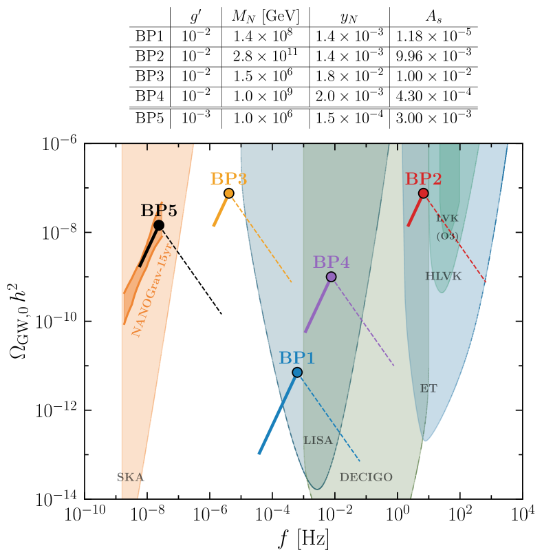
Figure 2: Benchmark IGW spectra from the eMD epoch driven by leptogenesis. The different lines corresponds to the benchmark points of the model parameter space reported in the top table. Except for BP5, they all assume $g^{\prime}=10^{-2}$ and $A_{\rm s}=A_{\rm s}^{\rm min}$ defined in Eq. (4). The full parameter space for $g^{\prime}=10^{-2}$ is provided in Fig. 1. The dashed lines display the extrapolation of the GW spectrum as $f^{-1}$. We also show the NANOGrav 15yr results [18] for the tentative nHz GW background [14, 15, 16, 17, 18]. The shaded regions represent the LVK bound [8] and the power-law integrated sensitivity curves for different experiments [92, 93].

In Fig. 3, we explore the correspondence between $M_{N}$ and $f_{\rm high}$ including $A_{\rm s}$. Specifically, the regions in different colors represent the allowed parameter space obtained by fixing the leptogenesis scale and varying the other parameters as $g^{\prime}\in[10^{-3.0},\,10^{-1.5}]$, $y_{N}\in[\sqrt{2g^{\prime 3}}\,,2\sqrt{g^{\prime}}]$ and $A_{\rm s}\in[\max(10^{-9},A_{\rm s}^{\rm min}),\,10^{-2}]$. We find that smaller $g^{\prime}$ values imply longer duration of the eMD and smaller $T_{\mathrm{dec}}$ without jeopardizing their parametric dependence on the $M_{N}$. This is evident from the enlarged regions corresponding to smaller $g^{\prime}$ values in Fig. 3. In this framework, leptogenesis scales $M_{N}\lesssim 10^{12}~\mathrm{GeV}$ have less discovery potential with IGWs owing to the constraint $v_{\phi}\leq v_{\phi}^{\rm max}$ and $A_{\rm s}\lesssim 10^{-2}$.

Let us also highlight two novel features of our leptogenesis framework. First, in this model, the leptogenesis scale $M_{N}$ is much higher than $T_{\rm dom}$. Therefore, in the computation of the BAU, one must account for the dilution factor $\Delta\simeq T_{\rm dec}/T_{\rm dom}$. The final value of the baryon-to-photon ratio in this case reads $\eta_{B}\simeq 10^{-3}\left(\frac{3m_{\nu}M_{Ni}}{8\pi v_{h}^{2}\delta}\right)\Delta$, where $\delta=(M_{Ni}-M_{Nj})/M_{Ni}$ accounts for the quasi-degeneracy among the RHNs [56, 77]. Requiring the observed value $\eta_{B}\simeq 6.3\times 10^{-10}$ and using Eq. (4), one finds $\delta\simeq 0.2\left(\frac{M_{Ni}}{10^{9}\,\mathrm{GeV}}\right)\sqrt{A_{\rm s}^{\rm min}}$. This implies that strong (weak) amplitude GWs are associated with weakly (strongly) quasi-degenerate RHNs. Second, since the GW frequency is sensitive to the leptogenesis scale, it follows that different flavor regimes, characterized by $M_{N}$ [4, 5, 6, 7], produce GWs at varying frequencies. This is significant because obtaining observable signatures through low-energy neutrino measurements typically requires imposing additional symmetries on the theory [94, 95, 96].

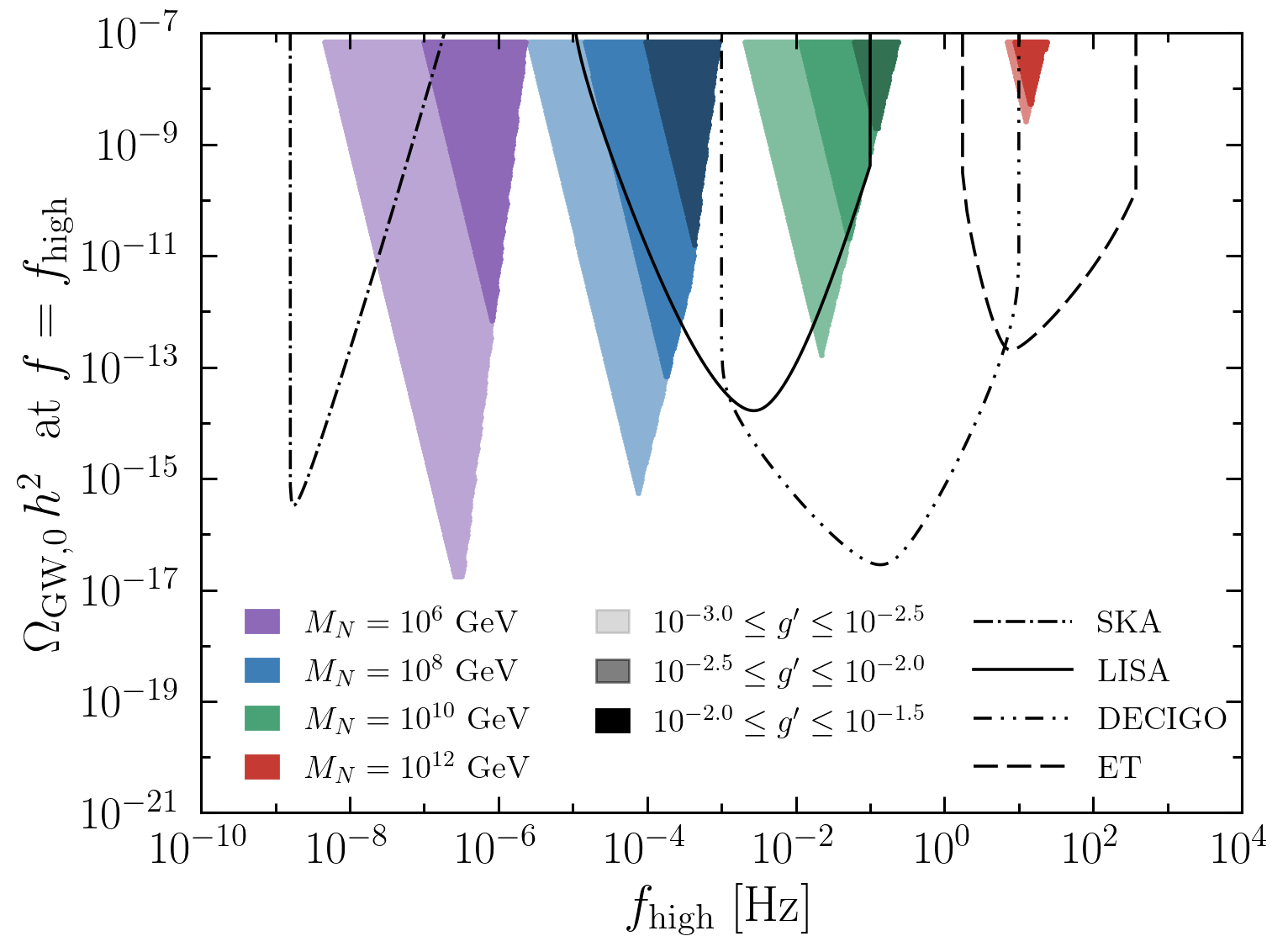
Figure 3: Allowed values for the GW amplitude in Eq. (6) computed at the peak frequency in Eq. (7), in case of different leptogenesis scales $M_{N}$ from $10^{6}~{\rm GeV}$ (left) to $10^{12}~{\rm GeV}$ (right). The color shading correspond to different intervals for the gauge coupling, with $A_{\rm s}\in[\max(10^{-9},A_{\rm s}^{\rm min}),\,10^{-2}]$. The black lines from left to right show the sensitivity of SKA, LISA, DECIGO, and ET detectors, respectively.

PBHs could be an additional signature of our scenario. Using the results of Refs. [81, 82] for the collapse of fluctuations in an eMD era, we see that amplitudes as low as $A_{\rm s}\sim 10^{-4}$ could lead to significant formation of light PBHs (see e.g. Fig. 4 and 7 of Ref. [82]), which are possible candidates for dark matter. As the PBH fraction and mass depend on the duration and end of the eMD era, we leave a detailed study for future work. We caution though that there are still several uncertainties in PBH calculations, see e.g. Refs. [83, 97, 98], and that the PBH abundance is highly sensitive to primordial non-Gaussianities [99, 100, 101, 102].

In conclusion, with this Letter, we connected two seemingly unrelated phenomena: leptogenesis and IGWs. Our results go beyond the simple leptogenesis model considered here. Indeed, various seesaw mechanisms and leptogenesis models share similar Lagrangian constructions [103], likely containing long-lived fields. Thus, any beyond-the-Standard-Model physics framework involving an eMD epoch can be readily explored through Eq.s (4) and (6). Moreover, simple leptogenesis frameworks, as the one discussed here, might also produce cosmic strings that radiate GWs [85, 77], though a detailed study will be presented elsewhere.

It is remarkable that, assuming our leptogenesis model, a detection of such IGW background selects a preferred island in the parameter space and excludes all the rest. In the worst case scenario, even the absence of a GW signal constrains a significant region of the leptogenesis parameter space, inaccessible otherwise.

Acknowledgements.  We thank Satyabrata Datta and Gennaro Miele for insightful discussions. MC, RS, and NS acknowledge the support of the project TAsP (Theoretical Astroparticle Physics) funded by the Istituto Nazionale di Fisica Nucleare (INFN). The work of NS is further supported by the research grant number 2022E2J4RK “PANTHEON: Perspectives in Astroparticle and Neutrino THEory with Old and New Messengers” under the program PRIN 2022 funded by the Italian Ministero dell’Università e della Ricerca (MUR). GD is supported by the DFG under the Emmy-Noether program, project number 496592360, and by the JSPS KAKENHI grant No. JP24K00624. TP acknowledges the contribution of the LISA Cosmology Working Group as well as support of the INFN Sezione di Napoli through the project QGSKY.

References

- Fukugita and Yanagida [1986] M. Fukugita and T. Yanagida, Baryogenesis Without Grand Unification, Phys. Lett. B 174, 45 (1986).
- Davidson et al. [2008] S. Davidson, E. Nardi, and Y. Nir, Leptogenesis, Phys. Rept. 466, 105 (2008), arXiv:0802.2962 [hep-ph] .
- Buchmuller et al. [2005] W. Buchmuller, P. Di Bari, and M. Plumacher, Leptogenesis for pedestrians, Annals Phys. 315, 305 (2005), arXiv:hep-ph/0401240 .
- Abada et al. [2006] A. Abada, S. Davidson, A. Ibarra, F. X. Josse-Michaux, M. Losada, and A. Riotto, Flavour Matters in Leptogenesis, JHEP 09, 010, arXiv:hep-ph/0605281 .
- Nardi et al. [2006] E. Nardi, Y. Nir, E. Roulet, and J. Racker, The Importance of flavor in leptogenesis, JHEP 01, 164, arXiv:hep-ph/0601084 .
- Blanchet and Di Bari [2007] S. Blanchet and P. Di Bari, Flavor effects on leptogenesis predictions, JCAP 03, 018, arXiv:hep-ph/0607330 .
- Pascoli et al. [2007a] S. Pascoli, S. T. Petcov, and A. Riotto, Leptogenesis and Low Energy CP Violation in Neutrino Physics, Nucl. Phys. B 774, 1 (2007a), arXiv:hep-ph/0611338 .
- Abbott et al. [2021] R. Abbott et al. (KAGRA, Virgo, LIGO Scientific), Upper limits on the isotropic gravitational-wave background from Advanced LIGO and Advanced Virgo’s third observing run, Phys. Rev. D 104, 022004 (2021), arXiv:2101.12130 [gr-qc] .
- Sathyaprakash et al. [2012] B. Sathyaprakash et al., Scientific Objectives of Einstein Telescope, Class. Quant. Grav. 29, 124013 (2012), [Erratum: Class.Quant.Grav. 30, 079501 (2013)], arXiv:1206.0331 [gr-qc] .
- Amaro-Seoane et al. [2017] P. Amaro-Seoane et al. (LISA), Laser Interferometer Space Antenna, (2017), arXiv:1702.00786 [astro-ph.IM] .
- Yagi and Seto [2011] K. Yagi and N. Seto, Detector configuration of DECIGO/BBO and identification of cosmological neutron-star binaries, Phys. Rev. D 83, 044011 (2011), [Erratum: Phys.Rev.D 95, 109901 (2017)], arXiv:1101.3940 [astro-ph.CO] .
- Weltman et al. [2020] A. Weltman et al., Fundamental physics with the Square Kilometre Array, Publ. Astron. Soc. Austral. 37, e002 (2020), arXiv:1810.02680 [astro-ph.CO] .
- Sesana et al. [2021] A. Sesana et al., Unveiling the gravitational universe at -Hz frequencies, Exper. Astron. 51, 1333 (2021), arXiv:1908.11391 [astro-ph.IM] .
- Antoniadis et al. [2023] J. Antoniadis et al. (EPTA, InPTA:), The second data release from the European Pulsar Timing Array - III. Search for gravitational wave signals, Astron. Astrophys. 678, A50 (2023), arXiv:2306.16214 [astro-ph.HE] .
- Reardon et al. [2023] D. J. Reardon et al., Search for an Isotropic Gravitational-wave Background with the Parkes Pulsar Timing Array, Astrophys. J. Lett. 951, L6 (2023), arXiv:2306.16215 [astro-ph.HE] .
- Xu et al. [2023] H. Xu et al., Searching for the Nano-Hertz Stochastic Gravitational Wave Background with the Chinese Pulsar Timing Array Data Release I, Res. Astron. Astrophys. 23, 075024 (2023), arXiv:2306.16216 [astro-ph.HE] .
- Antoniadis et al. [2024] J. Antoniadis et al. (EPTA, InPTA), The second data release from the European Pulsar Timing Array - IV. Implications for massive black holes, dark matter, and the early Universe, Astron. Astrophys. 685, A94 (2024), arXiv:2306.16227 [astro-ph.CO] .
- Afzal et al. [2023] A. Afzal et al. (NANOGrav), The NANOGrav 15 yr Data Set: Search for Signals from New Physics, Astrophys. J. Lett. 951, L11 (2023), arXiv:2306.16219 [astro-ph.HE] .
- Flauger et al. [2021] R. Flauger, N. Karnesis, G. Nardini, M. Pieroni, A. Ricciardone, and J. Torrado, Improved reconstruction of a stochastic gravitational wave background with LISA, JCAP 01, 059, arXiv:2009.11845 [astro-ph.CO] .
- Tomita [1967] K. Tomita, Non-Linear Theory of Gravitational Instability in the Expanding Universe, Progress of Theoretical Physics 37, 831 (1967), https://academic.oup.com/ptp/article-pdf/37/5/831/5234391/37-5-831.pdf .
- Matarrese et al. [1993] S. Matarrese, O. Pantano, and D. Saez, A General relativistic approach to the nonlinear evolution of collisionless matter, Phys. Rev. D 47, 1311 (1993).
- Matarrese et al. [1994] S. Matarrese, O. Pantano, and D. Saez, General relativistic dynamics of irrotational dust: Cosmological implications, Phys. Rev. Lett. 72, 320 (1994), arXiv:astro-ph/9310036 .
- Matarrese et al. [1998] S. Matarrese, S. Mollerach, and M. Bruni, Second order perturbations of the Einstein-de Sitter universe, Phys. Rev. D 58, 043504 (1998), arXiv:astro-ph/9707278 .
- Mollerach et al. [2004] S. Mollerach, D. Harari, and S. Matarrese, CMB polarization from secondary vector and tensor modes, Phys. Rev. D 69, 063002 (2004), arXiv:astro-ph/0310711 .
- Ananda et al. [2007] K. N. Ananda, C. Clarkson, and D. Wands, The Cosmological gravitational wave background from primordial density perturbations, Phys. Rev. D 75, 123518 (2007), arXiv:gr-qc/0612013 .
- Baumann et al. [2007] D. Baumann, P. J. Steinhardt, K. Takahashi, and K. Ichiki, Gravitational Wave Spectrum Induced by Primordial Scalar Perturbations, Phys. Rev. D 76, 084019 (2007), arXiv:hep-th/0703290 .
- Domènech [2021] G. Domènech, Scalar Induced Gravitational Waves Review, Universe 7, 398 (2021), arXiv:2109.01398 [gr-qc] .
- Assadullahi and Wands [2009] H. Assadullahi and D. Wands, Gravitational waves from an early matter era, Phys. Rev. D 79, 083511 (2009), arXiv:0901.0989 [astro-ph.CO] .
- Jedamzik et al. [2010a] K. Jedamzik, M. Lemoine, and J. Martin, Collapse of Small-Scale Density Perturbations during Preheating in Single Field Inflation, JCAP 09, 034, arXiv:1002.3039 [astro-ph.CO] .
- Jedamzik et al. [2010b] K. Jedamzik, M. Lemoine, and J. Martin, Generation of gravitational waves during early structure formation between cosmic inflation and reheating, Journal of Cosmology and Astroparticle Physics 2010 (04), 021–021.
- Alabidi et al. [2013] L. Alabidi, K. Kohri, M. Sasaki, and Y. Sendouda, Observable induced gravitational waves from an early matter phase, JCAP 05, 033, arXiv:1303.4519 [astro-ph.CO] .
- Kohri and Terada [2018] K. Kohri and T. Terada, Semianalytic calculation of gravitational wave spectrum nonlinearly induced from primordial curvature perturbations, Phys. Rev. D 97, 123532 (2018), arXiv:1804.08577 [gr-qc] .
- Inomata et al. [2019a] K. Inomata, K. Kohri, T. Nakama, and T. Terada, Enhancement of Gravitational Waves Induced by Scalar Perturbations due to a Sudden Transition from an Early Matter Era to the Radiation Era, Phys. Rev. D 100, 043532 (2019a), [Erratum: Phys.Rev.D 108, 049901 (2023)], arXiv:1904.12879 [astro-ph.CO] .
- Inomata et al. [2019b] K. Inomata, K. Kohri, T. Nakama, and T. Terada, Gravitational Waves Induced by Scalar Perturbations during a Gradual Transition from an Early Matter Era to the Radiation Era, JCAP 10, 071, [Erratum: JCAP 08, E01 (2023)], arXiv:1904.12878 [astro-ph.CO] .
- Papanikolaou et al. [2021] T. Papanikolaou, V. Vennin, and D. Langlois, Gravitational waves from a universe filled with primordial black holes, JCAP 03, 053, arXiv:2010.11573 [astro-ph.CO] .
- Domènech et al. [2021] G. Domènech, C. Lin, and M. Sasaki, Gravitational wave constraints on the primordial black hole dominated early universe, JCAP 04, 062, [Erratum: JCAP 11, E01 (2021)], arXiv:2012.08151 [gr-qc] .
- Dalianis and Kouvaris [2021] I. Dalianis and C. Kouvaris, Gravitational waves from density perturbations in an early matter domination era, JCAP 07, 046, arXiv:2012.09255 [astro-ph.CO] .
- Das et al. [2022] S. Das, A. Maharana, and F. Muia, A faster growth of perturbations in an early matter dominated epoch: primordial black holes and gravitational waves, Mon. Not. Roy. Astron. Soc. 515, 13 (2022), arXiv:2112.11486 [astro-ph.CO] .
- Eggemeier et al. [2023] B. Eggemeier, J. C. Niemeyer, K. Jedamzik, and R. Easther, Stochastic gravitational waves from postinflationary structure formation, Phys. Rev. D 107, 043503 (2023), arXiv:2212.00425 [astro-ph.CO] .
- Flores et al. [2023] M. M. Flores, A. Kusenko, and M. Sasaki, Gravitational Waves from Rapid Structure Formation on Microscopic Scales before Matter-Radiation Equality, Phys. Rev. Lett. 131, 011003 (2023), arXiv:2209.04970 [astro-ph.CO] .
- Kawasaki and Murai [2024] M. Kawasaki and K. Murai, Enhancement of gravitational waves at Q-ball decay including non-linear density perturbations, JCAP 01, 050, arXiv:2308.13134 [astro-ph.CO] .
- Basilakos et al. [2024] S. Basilakos, D. V. Nanopoulos, T. Papanikolaou, E. N. Saridakis, and C. Tzerefos, Induced gravitational waves from flipped SU(5) superstring theory at nHz, Phys. Lett. B 849, 138446 (2024), arXiv:2309.15820 [astro-ph.CO] .
- Tzerefos et al. [2025] C. Tzerefos, T. Papanikolaou, S. Basilakos, E. N. Saridakis, and N. E. Mavromatos, Gravitational wave signatures from reheating in axion-Chern-Simons running-vacuum cosmology, Phys. Rev. D 111, 043523 (2025), arXiv:2411.14223 [gr-qc] .
- Fernandez et al. [2024] N. Fernandez, J. W. Foster, B. Lillard, and J. Shelton, Stochastic Gravitational Waves from Early Structure Formation, Phys. Rev. Lett. 133, 111002 (2024), arXiv:2312.12499 [astro-ph.CO] .
- Pearce et al. [2024] M. Pearce, L. Pearce, G. White, and C. Balazs, Gravitational wave signals from early matter domination: interpolating between fast and slow transitions, JCAP 06, 021, arXiv:2311.12340 [astro-ph.CO] .
- Padilla et al. [2024] L. E. Padilla, J. C. Hidalgo, K. A. Malik, and D. Mulryne, Detecting the stochastic gravitational wave background from primordial black holes in slow-reheating scenarios, JCAP 12, 011, arXiv:2405.19271 [astro-ph.CO] .
- Dalianis and Kouvaris [2024] I. Dalianis and C. Kouvaris, Gravitational waves from collapse of pressureless matter in the early universe, JCAP 10, 006, arXiv:2403.15126 [astro-ph.CO] .
- Kawasaki et al. [1999] M. Kawasaki, K. Kohri, and N. Sugiyama, Cosmological constraints on late time entropy production, Phys. Rev. Lett. 82, 4168 (1999), arXiv:astro-ph/9811437 .
- Kawasaki et al. [2000] M. Kawasaki, K. Kohri, and N. Sugiyama, MeV scale reheating temperature and thermalization of neutrino background, Phys. Rev. D 62, 023506 (2000), arXiv:astro-ph/0002127 .
- Hannestad [2004] S. Hannestad, What is the lowest possible reheating temperature?, Phys. Rev. D 70, 043506 (2004), arXiv:astro-ph/0403291 .
- Hasegawa et al. [2019] T. Hasegawa, N. Hiroshima, K. Kohri, R. S. L. Hansen, T. Tram, and S. Hannestad, MeV-scale reheating temperature and thermalization of oscillating neutrinos by radiative and hadronic decays of massive particles, JCAP 12, 012, arXiv:1908.10189 [hep-ph] .
- Grohs and Fuller [2023] E. Grohs and G. M. Fuller, Big Bang Nucleosynthesis, in Handbook of Nuclear Physics, edited by I. Tanihata, H. Toki, and T. Kajino (2023) pp. 1–21, arXiv:2301.12299 [astro-ph.CO] .
- Davidson [1979] A. Davidson, Phys. Rev. D 20, 776 (1979).
- Marshak and Mohapatra [1980] R. E. Marshak and R. N. Mohapatra, Quark - Lepton Symmetry and B-L as the U(1) Generator of the Electroweak Symmetry Group, Phys. Lett. B 91, 222 (1980).
- Buchmüller et al. [2013] W. Buchmüller, V. Domcke, K. Kamada, and K. Schmitz, The Gravitational Wave Spectrum from Cosmological Breaking, JCAP 10, 003, arXiv:1305.3392 [hep-ph] .
- Pilaftsis and Underwood [2004] A. Pilaftsis and T. E. J. Underwood, Resonant leptogenesis, Nucl. Phys. B 692, 303 (2004), arXiv:hep-ph/0309342 .
- Minkowski [1977] P. Minkowski, at a Rate of One Out of Muon Decays?, Phys. Lett. B 67, 421 (1977).
- Gell-Mann et al. [1979] M. Gell-Mann, P. Ramond, and R. Slansky, Complex Spinors and Unified Theories, Conf. Proc. C 790927, 315 (1979), arXiv:1306.4669 [hep-th] .
- Yanagida [1980] T. Yanagida, Horizontal Symmetry and Masses of Neutrinos, Prog. Theor. Phys. 64, 1103 (1980).
- Mohapatra [1986] R. N. Mohapatra, Mechanism for Understanding Small Neutrino Mass in Superstring Theories, Phys. Rev. Lett. 56, 561 (1986).
- Linde [1979] A. D. Linde, Phase Transitions in Gauge Theories and Cosmology, Rept. Prog. Phys. 42, 389 (1979).
- Kibble [1980] T. W. B. Kibble, Some Implications of a Cosmological Phase Transition, Phys. Rept. 67, 183 (1980).
- Quiros [1999] M. Quiros, Finite temperature field theory and phase transitions, in ICTP Summer School in High-Energy Physics and Cosmology (1999) pp. 187–259, arXiv:hep-ph/9901312 .
- Caprini et al. [2016] C. Caprini et al., Science with the space-based interferometer eLISA. II: Gravitational waves from cosmological phase transitions, JCAP 04, 001, arXiv:1512.06239 [astro-ph.CO] .
- Hindmarsh et al. [2021] M. B. Hindmarsh, M. Lüben, J. Lumma, and M. Pauly, Phase transitions in the early universe, SciPost Phys. Lect. Notes 24, 1 (2021), arXiv:2008.09136 [astro-ph.CO] .
- Masso et al. [2005] E. Masso, F. Rota, and G. Zsembinszki, Scalar field oscillations contributing to dark energy, Phys. Rev. D 72, 084007 (2005), arXiv:astro-ph/0501381 .
- Datta and Samanta [2022] S. Datta and R. Samanta, Gravitational waves-tomography of Low-Scale-Leptogenesis, JHEP 11, 159, arXiv:2208.09949 [hep-ph] .
- Gross et al. [2016] C. Gross, O. Lebedev, and M. Zatta, Higgs–inflaton coupling from reheating and the metastable Universe, Phys. Lett. B 753, 178 (2016), arXiv:1506.05106 [hep-ph] .
- Enqvist et al. [2016] K. Enqvist, M. Karciauskas, O. Lebedev, S. Rusak, and M. Zatta, Postinflationary vacuum instability and Higgs-inflaton couplings, JCAP 11, 025, arXiv:1608.08848 [hep-ph] .
- Chianese et al. [2024] M. Chianese, S. Datta, R. Samanta, and N. Saviano, Tomography of flavoured leptogenesis with primordial blue gravitational waves, JCAP 11, 051, arXiv:2405.00641 [hep-ph] .
- Holdom [1986] B. Holdom, Two U(1)’s and Epsilon Charge Shifts, Phys. Lett. B 166, 196 (1986).
- Cheung et al. [2009] C. Cheung, J. T. Ruderman, L.-T. Wang, and I. Yavin, Kinetic Mixing as the Origin of Light Dark Scales, Phys. Rev. D 80, 035008 (2009), arXiv:0902.3246 [hep-ph] .
- Gherghetta et al. [2019] T. Gherghetta, J. Kersten, K. Olive, and M. Pospelov, Evaluating the price of tiny kinetic mixing, Phys. Rev. D 100, 095001 (2019), arXiv:1909.00696 [hep-ph] .
- Hook et al. [2011] A. Hook, E. Izaguirre, and J. G. Wacker, Model Independent Bounds on Kinetic Mixing, Adv. High Energy Phys. 2011, 859762 (2011), arXiv:1006.0973 [hep-ph] .
- Blasi et al. [2020] S. Blasi, V. Brdar, and K. Schmitz, Fingerprint of low-scale leptogenesis in the primordial gravitational-wave spectrum, Phys. Rev. Res. 2, 043321 (2020), arXiv:2004.02889 [hep-ph] .
- Han and Wang [2017] T. Han and X. Wang, Radiative Decays of the Higgs Boson to a Pair of Fermions, JHEP 10, 036, arXiv:1704.00790 [hep-ph] .
- Chianese et al. [2025] M. Chianese, S. Datta, G. Miele, R. Samanta, and N. Saviano, Probing flavored regimes of leptogenesis with gravitational waves from cosmic strings, Phys. Rev. D 111, L041305 (2025), arXiv:2406.01231 [hep-ph] .
- Samanta [2025] R. Samanta, Probing Leptogenesis at LISA: A Fisher analysis, (2025), arXiv:2503.09884 [hep-ph] .
- Loureiro et al. [2019] A. Loureiro et al., On The Upper Bound of Neutrino Masses from Combined Cosmological Observations and Particle Physics Experiments, Phys. Rev. Lett. 123, 081301 (2019), arXiv:1811.02578 [astro-ph.CO] .
- Aker et al. [2022] M. Aker et al. (KATRIN), Direct neutrino-mass measurement with sub-electronvolt sensitivity, Nature Phys. 18, 160 (2022), arXiv:2105.08533 [hep-ex] .
- Harada et al. [2016] T. Harada, C.-M. Yoo, K. Kohri, K.-i. Nakao, and S. Jhingan, Primordial black hole formation in the matter-dominated phase of the Universe, Astrophys. J. 833, 61 (2016), arXiv:1609.01588 [astro-ph.CO] .
- Ballesteros et al. [2020] G. Ballesteros, J. Rey, and F. Rompineve, Detuning primordial black hole dark matter with early matter domination and axion monodromy, JCAP 06, 014, arXiv:1912.01638 [astro-ph.CO] .
- De Luca et al. [2022] V. De Luca, G. Franciolini, A. Kehagias, P. Pani, and A. Riotto, Primordial black holes in matter-dominated eras: The role of accretion, Phys. Lett. B 832, 137265 (2022), arXiv:2112.02534 [astro-ph.CO] .
- Sasaki et al. [2018] M. Sasaki, T. Suyama, T. Tanaka, and S. Yokoyama, Primordial black holes—perspectives in gravitational wave astronomy, Class. Quant. Grav. 35, 063001 (2018), arXiv:1801.05235 [astro-ph.CO] .
- Dror et al. [2020] J. A. Dror, T. Hiramatsu, K. Kohri, H. Murayama, and G. White, Testing the Seesaw Mechanism and Leptogenesis with Gravitational Waves, Phys. Rev. Lett. 124, 041804 (2020), arXiv:1908.03227 [hep-ph] .
- Samanta and Datta [2021] R. Samanta and S. Datta, Gravitational wave complementarity and impact of NANOGrav data on gravitational leptogenesis, JHEP 05, 211, arXiv:2009.13452 [hep-ph] .
- Datta et al. [2021] S. Datta, A. Ghosal, and R. Samanta, Baryogenesis from ultralight primordial black holes and strong gravitational waves from cosmic strings, JCAP 08, 021, arXiv:2012.14981 [hep-ph] .
- Adamek et al. [2016] J. Adamek, D. Daverio, R. Durrer, and M. Kunz, gevolution: a cosmological N-body code based on General Relativity, JCAP 07, 053, arXiv:1604.06065 [astro-ph.CO] .
- Ade et al. [2016] P. A. R. Ade et al. (Planck), Planck 2015 results. XIII. Cosmological parameters, Astron. Astrophys. 594, A13 (2016), arXiv:1502.01589 [astro-ph.CO] .
- Özsoy and Tasinato [2023] O. Özsoy and G. Tasinato, Inflation and Primordial Black Holes, Universe 9, 203 (2023), arXiv:2301.03600 [astro-ph.CO] .
- Burgess et al. [2008] C. P. Burgess, J. P. Conlon, L.-Y. Hung, C. H. Kom, A. Maharana, and F. Quevedo, Continuous Global Symmetries and Hyperweak Interactions in String Compactifications, JHEP 07, 073, arXiv:0805.4037 [hep-th] .
- Thrane and Romano [2013] E. Thrane and J. D. Romano, Sensitivity curves for searches for gravitational-wave backgrounds, Phys. Rev. D 88, 124032 (2013), arXiv:1310.5300 [astro-ph.IM] .
- Schmitz [2021] K. Schmitz, New Sensitivity Curves for Gravitational-Wave Signals from Cosmological Phase Transitions, JHEP 01, 097, arXiv:2002.04615 [hep-ph] .
- Pascoli et al. [2007b] S. Pascoli, S. T. Petcov, and A. Riotto, Leptogenesis and Low Energy CP Violation in Neutrino Physics, Nucl. Phys. B 774, 1 (2007b), arXiv:hep-ph/0611338 .
- Akhmedov et al. [2003] E. K. Akhmedov, M. Frigerio, and A. Y. Smirnov, Probing the seesaw mechanism with neutrino data and leptogenesis, JHEP 09, 021, arXiv:hep-ph/0305322 .
- Bertuzzo et al. [2009] E. Bertuzzo, P. Di Bari, F. Feruglio, and E. Nardi, Flavor symmetries, leptogenesis and the absolute neutrino mass scale, JHEP 11, 036, arXiv:0908.0161 [hep-ph] .
- Saito et al. [2024] D. Saito, T. Harada, Y. Koga, and C.-M. Yoo, Revisiting spins of primordial black holes in a matter-dominated era based on peak theory, JCAP 11, 064, arXiv:2409.00435 [gr-qc] .
- Ianniccari et al. [2024] A. Ianniccari, A. J. Iovino, A. Kehagias, D. Perrone, and A. Riotto, Primordial black hole abundance: The importance of broadness, Phys. Rev. D 109, 123549 (2024), arXiv:2402.11033 [astro-ph.CO] .
- Young and Byrnes [2013] S. Young and C. T. Byrnes, Primordial black holes in non-Gaussian regimes, JCAP 08, 052, arXiv:1307.4995 [astro-ph.CO] .
- Franciolini et al. [2018] G. Franciolini, A. Kehagias, S. Matarrese, and A. Riotto, Primordial Black Holes from Inflation and non-Gaussianity, JCAP 03, 016, arXiv:1801.09415 [astro-ph.CO] .
- Ferrante et al. [2023] G. Ferrante, G. Franciolini, A. Iovino, Junior., and A. Urbano, Primordial non-Gaussianity up to all orders: Theoretical aspects and implications for primordial black hole models, Phys. Rev. D 107, 043520 (2023), arXiv:2211.01728 [astro-ph.CO] .
- Pi [2024] S. Pi, Non-Gaussianities in primordial black hole formation and induced gravitational waves, (2024), arXiv:2404.06151 [astro-ph.CO] .
- Hettmansperger et al. [2011] H. Hettmansperger, M. Lindner, and W. Rodejohann, Phenomenological Consequences of sub-leading Terms in See-Saw Formulas, JHEP 04, 123, arXiv:1102.3432 [hep-ph] .