Graph-based Semi-supervised and Unsupervised Methods for Local Clustering

Abstract

Local clustering aims to identify specific substructures within a large graph without requiring full knowledge of the entire graph. These substructures are typically small compared to the overall graph, enabling the problem to be approached by finding a sparse solution to a linear system associated with the graph Laplacian. In this work, we first propose a method for identifying specific local clusters when very few labeled data is given, which we term semi-supervised local clustering. We then extend this approach to the unsupervised setting when no prior information on labels is available. The proposed methods involve randomly sampling the graph, applying diffusion through local cluster extraction, then examining the overlap among the results to find each cluster. We establish the co-membership conditions for any pair of nodes and rigorously prove the correctness of our methods. Additionally, we conduct extensive experiments to demonstrate that the proposed methods achieve state-of-the-arts results in the low-label rates regime.

1 Introduction

The ability to learn from data by uncovering its underlying patterns and grouping it into distinct clusters based on latent similarities and differences is a central focus in machine learning and artificial intelligence. Over the past few decades, traditional clustering problems have been extensively studied as an unsupervised learning task, leading to the development of a wide range of foundational algorithms,, such as $k$-means clustering (MacQueen, 1967), density-based clustering (Ester et al., 1996), spectral clustering (Ng et al., 2001; Zelnik-Manor and Perona, 2004), hierarchical clustering (Nielsen, 2016) and regularized $k$-means (Kang et al., 2011). These foundational methods have, in turn, inspired numerous variants and adaptations tailored to specific data characteristics or application domains.

Researchers have also developed semi-supervised learning approach for clustering, which leverages both labeled and unlabeled data in various learning tasks. One of the most commonly used methods in graph-based semi-supervised learning is Laplace learning (Zhu et al., 2003). Note that Laplacian learning sometimes is also called Label propagation (Zhu and Ghahramani, 2002), which seeks a graph harmonic function that extends the labels. Laplacian learning and its variants have been extensively applied in semi-supervised learning tasks (Zhou et al., 2004a, b, 2005; Ando and Zhang, 2007; Kang et al., 2014). A key challenge with Laplacian learning type of algorithms is their poor performance in the low-label rates regime. To address this, recent approaches have explored $p$-Laplacian learning (El Alaoui et al., 2016; Flores et al., 2022), higher order Laplacian regularization (Zhou and Belkin, 2011), weighted nonlocal Laplacians (Shi et al., 2017), properly weighted Laplacian (Calder and Slepcev, 2019), and Poisson learning (Calder et al., 2020).

Those aforementioned clustering algorithms, no matter whether unsupervised or semi-supervised, are all global clustering algorithms in nature, recovering all cluster structures simultaneously. However, real-world applications often require identifying only specific substructures within large, complex networks. For example, in a social network, an individual may only be interested in connecting with others who share similar interests, while disregarding the rest of individuals. In such cases, global clustering methods become inefficient, as they generate excessive redundant information rather than focusing on the relevant local patterns.

In this paper, we turn our focus to a more flexible clustering method called local clustering or local cluster extraction. Eluded by its name, local clustering focus only on finding one target cluster which contains those nodes of interest to us, and disregard the non-interest or background nodes. Researchers have investigated in this direction over the recent decades such as (Lang and Rao, 2004; Andersen et al., 2006; Kloster and Gleich, 2014; Spielman and Teng, 2013; Andersen et al., 2016; Veldt et al., 2019; Fountoulakis et al., 2020). More recently, inspired by the idea of compressive sensing, the authors in (Lai and Mckenzie, 2020; Lai and Shen, 2023; Shen et al., 2023) proposed a novel perspective for local clustering by finding the target cluster via solving a sparse solution to a linear system associated with the graph Laplacian matrix. (Shen, 2024) also provides a comprehensive summary of the compressive sensing based clustering approaches. Such approaches can be applied in medical imaging as demonstrated in (Hamel et al., 2024). Intuitively speaking, as local clustering only focus on finding “one cluster at a time”, it is flexible in practice and can be more efficient and effective than global clustering algorithms.

Besides such merits that local clustering algorithms possesses, one big downside of it is the necessity of having the initial nodes (we call them seeds) of interest as prior knowledge, and it also requires a good estimate of the target cluster size. The seeds information is sometimes very limited and even unavailable, which makes local clustering algorithm less popular. We propose a clustering method which requires very few seeds (semi-supervised case) or no seeds (unsupervised case), see Figure 1 and 2 for illustration. We provide a detailed discussion of the procedure, with analysis on the correctness of the proposed method. The main contributions of our work are the following.

1. We propose a semi-supervised (with very few labeled data) and an unsupervised (no labeled data) local clustering methods which outperform the state-of-the-arts local and non-local clustering methods in most cases.

2. We establish the co-membership conditions for any pair of nodes in the unsupervised case, and then prove the correctness of our unsupervised method.

3. Our semi-supervised method can find all the clusters simultaneously which improves the “one cluster at a time” feature of local clustering algorithms in terms of efficiency. We provide extensive experiments with comparisons to show the effectiveness of our methods in the low-label rates regime.

The rest of the paper is organized as follows. In Section 2, we introduce the notation, background and preliminaries. In Section 3, we present step-by-step procedure of proposed methods in both semi-supervised and unsupervised settings, and prove their correctness under certain assumptions. In section 4, we show the experimental results of the proposed methods and compare them with the state-of-the-art semi-supervised clustering algorithms on various benchmark datasets. Finally, in Section 5, we make conclusion and discuss the limitation.

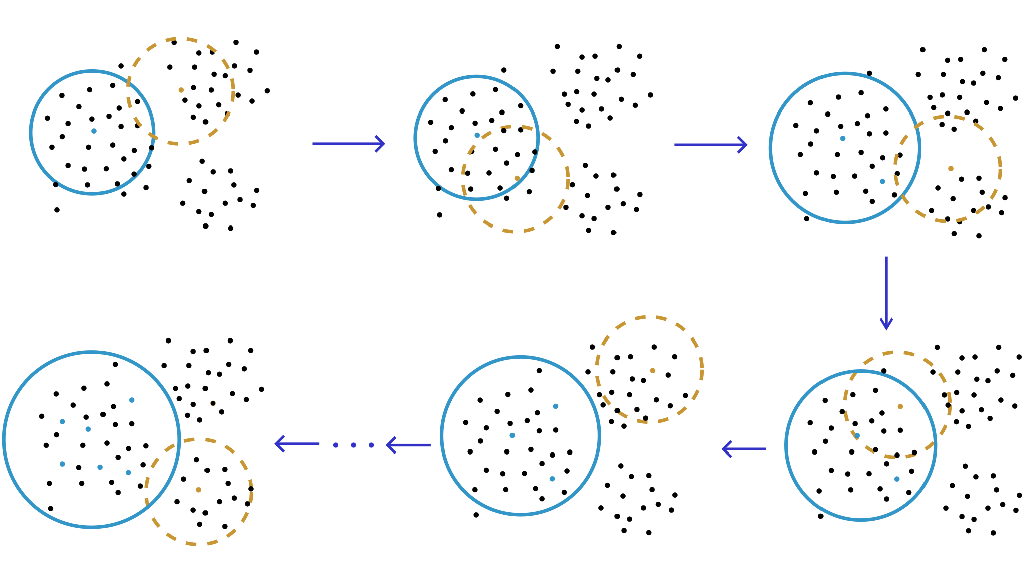
Figure 1: Illustration of semi-supervised local clustering method (SSLC) for a single cluster. Each subplot indicates one iteration (Blue points: seeds in $\Gamma_{1}$. Brown points: randomly sampled node in each iteration).

2 Background

2.1 Notations and Preliminaries

For a graph $G=(V,E)$, we use $V$ to denote the set of all nodes, and $E$ to denote the set of all edges. Suppose $G$ has $k$ non-overlapping underlying clusters $C_{1},C_{2},\cdots,C_{k}$, we use $n_{i}$ to denote the size of $C_{i}$ where $i=1,2,\cdots,k$, and use $n$ to denote the total size of graph $G$. Further, we use $A$ to denote the adjacency matrix (possibly weighted but non-negative) of graph $G$, and use $D$ to denote the diagonal matrix whose diagonal entries is the degree of the corresponding vertex. Moreover, we need the definition of graph Laplacian(s).

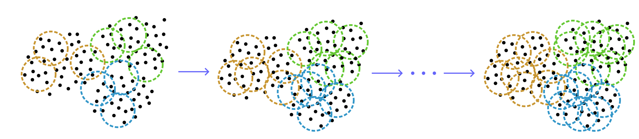
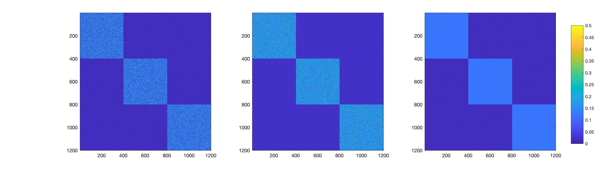
Figure 2: Illustration of unsupervised local clustering (USLC) procedure. Top row: each dashed circle represents one iteration of LCE generated from a randomly sampled node, we use different colors to indicate local clusters generated from nodes of different underlying clusters. Bottom row: Aggregated co-membership matrix.

Definition 1

The unnormalized graph Laplacian of graph G is defined as $L:=D-A$. The symmetric graph Laplacian of graph G is defined as $L_{sym}:=I-D^{-1/2}AD^{-1/2}$ and the random walk graph Laplacian is defined as $L_{rw}:=I-D^{-1}A$.

We mainly focus on $L_{rw}$ for the rest of discussion. To simplify the notation, we will use $L$ to denote $L_{rw}$. The following result is central to our proposed method for sparse-solution-based local clustering. We omit its proof by referring to (Von Luxburg, 2007).

Lemma 1

Let G be an undirected graph with non-negative weights. The multiplicity $k$ of the eigenvalue zero of $L\text{ }(L_{rw})$ equals to the number of connected components $C_{1},C_{2},\cdots,C_{k}$ in $G$, and the indicator vectors $\textbf{1}_{C_{1}},\cdots,\textbf{1}_{C_{k}}\in\mathbb{R}^{n}$ on these components span the kernel of $L\text{ }(L_{rw})$.

For the convenience of our discussion, let us introduce more notations . For a graph $G=(V,E)$ with certain underlying community structure, it is convenient to write $G=G^{in}\cup G^{out}$, where $G^{in}=(V,E^{in})$, $G^{out}=(V,E^{out})$. Here $E^{in}$ is the set of all intra-connection edges within the same community (cluster), $E^{out}$ is the remaining edges in $E$. Further, we use $A^{in}$ and $L^{in}$ to denote the adjacency matrix and Laplacian matrix associated with $G^{in}$ respectively. A summary of the notations being used throughout this paper is included in Table 5 in Appendix A.

Remark 1

We do not guarantee knowledge of the cluster to which each individual vertex belongs, meaning that $A^{in}$ and $L^{in}$ are not directly accessible. Instead, we only have access to $A$ and $L$.

2.2 Local Cluster Extraction (LCE) via Compressive Sensing

Let us first briefly introduce the idea Local Cluster Extraction (LCE), which applies the idea of compressive sensing (or sparse solution) technique to extract the target cluster in a semi-supervised manner. See also (Lai and Mckenzie, 2020; Lai and Shen, 2023; Shen et al., 2023) for references.

Suppose the graph $G$ consists of $k$ connected equal-size components $C_{1},\cdots,C_{k}$, in other words, there is no edge connection between different clusters, i.e., $L=L^{in}$. For illustration purpose, let us permute the matrix according to the membership of each node, then $L^{in}$ is in a block diagonal form i.e., all the off-diagnoal blocks equal to zero:

$$L=L^{in}=\left(\begin{array}[]{cccc}L^{in}_{C_{1}}&&&\\ &L^{in}_{C_{2}}&&\\ &&\ddots&\\ &&&L^{in}_{C_{k}}\\ \end{array}\right).$$ (1)

Suppose that the target cluster is $C_{1}$. By Lemma 1, $\{\mathbf{1}_{C_{1}},\cdots,\mathbf{1}_{C_{k}}\}$ forms a basis of the kernel $W_{0}$ of $L$. Note that all the $\mathbf{1}_{C_{i}}$ have disjoint supports, so for $\mathbf{w}\in W_{0}$ and $\mathbf{w}\neq 0$, we can write

$$\mathbf{w}=\sum_{i=1}^{k}\alpha_{i}\mathbf{1}_{C_{i}}$$ (2)

with some $\alpha_{i}\neq 0$. If we further have the prior knowledge that first node $v_{1}\in C_{1}$, then we can find the first cluster $C_{1}$ by solving

$$\min||\mathbf{w}||_{0}\quad\text{s.t.}\quad L^{in}\mathbf{w}=\mathbf{0}\quad\text{and}\quad w_{1}=1,$$ (3)

which gives the solution $\mathbf{w}=\mathbf{1}_{C_{1}}\in\mathbb{R}^{n}$ as desired. It is worthwhile to note that (3) is equivalent to

$$\min||\mathbf{w}||_{0}\quad\text{s.t.}\quad L_{-1}^{in}\mathbf{w}=-\ell_{1},$$ (4)

where $L_{-1}^{in}$ is a submatrix of $L^{in}$ with first column being removed, $\ell_{1}$ is the first column of $L^{in}$. The solution to (4) is $\mathbf{w}=\mathbf{1}_{C_{1}\setminus{v_{1}}}\in\mathbb{R}^{n-1}$ which encodes the same index information as the solution to (3). The benefit of having formulation (4) is that we can now solve it by compressive sensing algorithms. A brief introduction on compressive sensing and sparse solution technique is provided in Appendix D.

Algorithm 1 Semi-supervised Local Clustering (SSLC) for a Single Cluster

0: The adjacency matrix $A$ of an underlying graph $G$, the initial seed(s) $\Gamma_{1}$ for the target cluster $C_{1}$, the estimated size ${n}_{1}$, the number of resampling iteration $L$

0: desired output cluster $C_{1}^{\#}$

1: $\tilde{C}_{1}\leftarrow{\rm LCE}(A,{n}_{1},\Gamma_{1})$

2: for $\ell=1:L$ do

3:  $v\leftarrow$ randomly sampled seed node from $G$

4:  $C^{\#}\leftarrow{\rm LCE}(A,{n}_{1},v)$

5:  if $|\tilde{C}_{1}\cap C^{\#}|>0.5|C^{\#}|$ for some $s$ then

6:   $\Gamma_{1}\leftarrow\Gamma_{1}\cup\{v\}$

7:   $\tilde{C}_{1}\leftarrow{\rm LCE}(A,{n}_{1},\Gamma_{1})$

8:  end if

9: end for

10: $C_{1}^{\#}\leftarrow\tilde{C}_{1}$

Algorithm 2 Semi-supervised Local Clustering (SSLC) for Multiple Clusters

0: The adjacency matrix $A$ of an underlying graph $G$, the number of cluster $k$, the initial seed(s) $\Gamma_{s}$ for each cluster, the estimated size ${n}_{s}$ for each cluster, $s=1,\cdots,k$, the number of resampling iteration $L$

0: desired output clusters $C_{1}^{\#},\cdots,C_{k}^{\#}$

1: for $s=1:k$ do

2:  $\tilde{C}_{s}\leftarrow{\rm LCE}(A,{n}_{s},\Gamma_{s})$

3: end for

4: for $\ell=1:L$ do

5:  $v\leftarrow$ randomly sampled seed node from $G$

6:  $C^{\#}\leftarrow{\rm LCE}(A,\min\{n_{s}\}_{s\geq 1},v)$

7:  if $|\tilde{C}_{s}\cap C^{\#}|>0.5|C^{\#}|$ for some $s$ then

8:   $\Gamma_{s}\leftarrow\Gamma_{s}\cup\{v\}$

9:   $\tilde{C}_{s}\leftarrow{\rm LCE}(A,{n}_{s},\Gamma_{s})$

10:  end if

11: end for

12: for $s=1:k$ do

13:  $C_{s}^{\#}\leftarrow\tilde{C}_{s}$

14: end for

Remark 2

In practice, we cannot permute the matrix according to the nodes’ membership if we do not have access to the membership information. However, the sparse solution we get from solving (3) or (4) always gives the indices corresponding to the target cluster. Therefore, the permutation does not affect our analysis and clustering result.

When the graph is of large size, only knowing one node belonging to the target cluster may not be not enough. Our goal is to start from one (or a few) node(s), extract a small portion $U\subseteq C_{1}$, then remove the columns associated with $U$ from $L$ and formulate it the same way as (4). The idea for obtaining such an index set $U$ is based on a heuristic criterion coming from the random walk staring from the initial seeds. The above procedure is summarized in Algorithm 4 (CS-LCE or LCE (Shen et al., 2023)) in Appendix E. A more detailed analysis of LCE is also provided in Appendix E.

Let $\mathbf{x}^{*}$ be the solution to the unperturbed problem (8), and $\mathbf{x}^{\#}$ be the solution to the perturbed problem (7), we want to highlight the following Lemma 2, which is a crucial step in establishing the convergence result in LCE. We are able to relax the assumption from $\|\Delta L\|_{2}=O(n^{-1/2})$ (Shen et al., 2023) to $\|\Delta L\|_{2}=o(1)$. The proof of Lemma 2 is provided in Appendix F.

Lemma 2

Let $\Delta L:=L-L^{in}$. Suppose $U\subset C_{1}$ and $0.1|C_{1}|<|U|<0.9|C_{1}|$. Suppose further that $\|\Delta L\|_{2}=o(1)$ and $\left(\delta_{3(|C_{1}|-|U|)}(L)\right)^{\log(n)}=o(1)$. Then

$$\frac{\|\mathbf{x}^{\#}-\mathbf{x}^{*}\|_{2}}{\|\mathbf{x}^{*}\|_{2}}=o(1).$$ (5)

3 Proposed Methods

Let us formally state the two clustering tasks we are interested in.

1. Semi-supervised case: Given a graph $G=(V,E)$ with underlying cluster $C_{1},\cdots,C_{k}$ such that $V=\cup_{i=1}^{k}C_{i}$, $C_{i}\cap C_{j}=\emptyset$ for $1\leq i,j\leq k$, $i\neq j$.

   1. Suppose a very small portion of seeds $\Gamma_{1}\subset C_{1}$ is available, we would like to find all the nodes in the target cluster $C_{1}$.

   2. Suppose a very small portion of seeds $\Gamma_{i}\subset C_{i}$ is available for each $i=1,\cdots,k$, we would like to assign all nodes to their corresponding underlying clusters.

2. Unsupervised case: Given a graph $G=(V,E)$ with underlying cluster $C_{1},C_{2},\cdots$, where $V=\cup_{i\geq 1}C_{i}$, $C_{i}\cap C_{j}=\emptyset$ for all $i\neq j$. Assume neither the prior information about seeds nor the number of cluster $k$ is given, the goal is to assign all the nodes to their corresponding underlying clusters.

3.1 Assumptions

We make the following assumptions on the graph model.

Assumption 1

The non-zero entries in the diagonal block is much denser than the non-zero entries in the off-diagonal block (after the permutation according to the membership). More precisely, we assume the graph Laplacian of the graph $G$ satisfies $\|\Delta L\|_{2}=\|L-L^{in}\|_{2}=o(1)$.

Assumption 2

The number of cluster $k=O(1)\geq 2$. The size of each cluster is not too small or too large, i.e., there exist $n_{\min}=\Theta(n)$ and $n_{\max}=\Theta(n)$ such that $n_{\min}\leq n_{i}\leq n_{\max}$ for any $i\geq 1$.

Assumption 3

Each underlying cluster of the graph is asymptotically regular.

3.2 The Main Model

Let us explain the two models we propose, one for semi-supervised local clustering and the other for unsupervised local clustering.

3.2.1 Semi-supervised Local Clustering

Similar to the issue of Laplacian learning type of algorithms, local clustering approach such as LCE becomes less effective in the low label regime. In such case, we can extract more seeds from each cluster before applying LCE. We illustrate the idea in Figure 1. For simplicity, suppose we are only interested in finding the cluster $C_{1}$, which is the cluster in the left of those three clusters illustrated in the first subplot of Figure 1. The procedure of semi-supervised local clustering (SSLC) works as follows.

1. Given a graph $G$, and an initial set of seed(s) $\Gamma_{1}$ (indicated as the blue point in the first subplot), we first apply LCE to have a rough estimate $\tilde{C}_{1}$ (indicated by the solid blue circle) of $C_{1}$.

2. Randomly sample a node $v$ (the brown point in the first subplot) in $G$ and apply LCE to get a rough cluster around $v$ (indicated by the dashed brown circle). Then check the overlap between solid blue and dashed brown circle. If the overlap contains the majority of the nodes in the brown circle, then add $v$ into $\Gamma_{1}$, otherwise sample another node.

3. Continue this process and keep increasing the size of $\Gamma_{1}$ until a predetermined iteration number is reached (indicated in the process of from the second to the last subplots).

Algorithm 3 Unsupervised Local Clustering (USLC)

0: The adjacency matrix $A$ of an underlying graph $G$, the upper bound for the number of clusters $K$, the number of resampling iteration $L$

0: The desired clusters $C_{1}^{\#},C_{2}^{\#},\cdots$

1: initialize $s\leftarrow 1$

2: while $s<K$ or $|G|<n_{\min}$ do

3:  initialize the comembership matrix $M$ as zero matrix

4:  for $\ell=1:L$ do

5:   randomly sample a node $v$ from $G$ as seed

6:   $C^{\#}\leftarrow{\rm LCE}(A,n_{\min},v)$

7:   $M\leftarrow M+\frac{1}{L}\cdot{\rm comembership}(\mathbf{1}_{C^{\#}})$

8:  end for

9:  select a node $v$ uniformly random such that $M_{v,i}>\delta$ for some $i\neq v$, with some appropriate $\delta\in(0,1)$, then find all the $j$ such that $C_{s}^{\#}:=\{j:M_{v,j}>\delta$}

10:  Let $G^{(s)}$ be the subgraph spanned by $C_{s}^{\#}$

11:  $G\leftarrow G\setminus G^{(s)}$

12:  $s\leftarrow s+1$

13: end while

Note that the above procedure can be applied when more than one cluster is of interest without increasing the number of iterations. The procedures for the single cluster case and multiple clusters case are summarized in Algorithm 1 and 2 respectively. In this way, we are able to find more seeds based on the initial seeds, and the user can flexibly determine the number of seeds wanted by increasing or decreasing the number of iterations.

Remark 3

One notable advantage of Algorithm 2 is its ability to simultaneously identify all clusters, while previous method such as LCE can only detect one cluster at a time. This characteristic provides greater flexibility and makes Algorithm 2 significantly more efficient for practical applications, particularly when the number of clusters is large. This advantage is also reflected in the first and second columns of Figure 3.

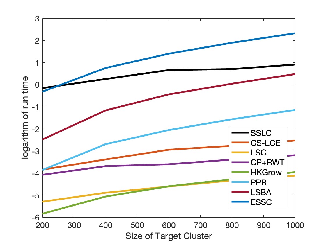
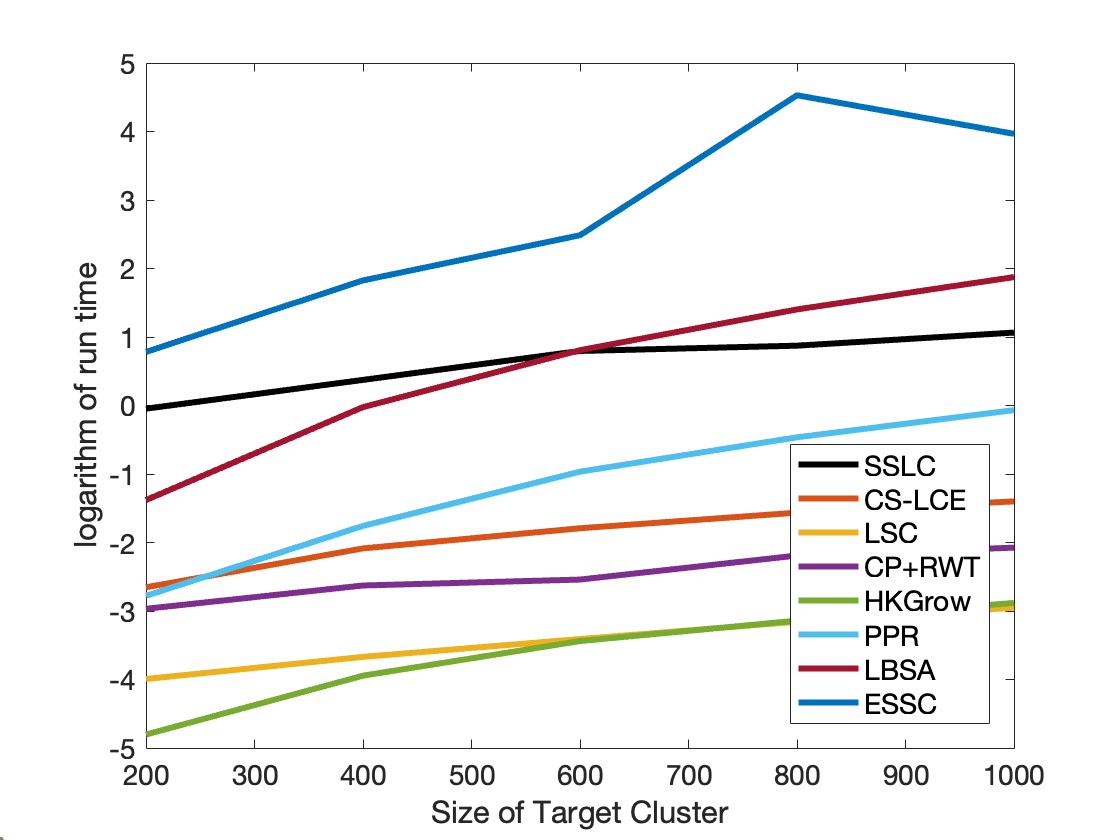
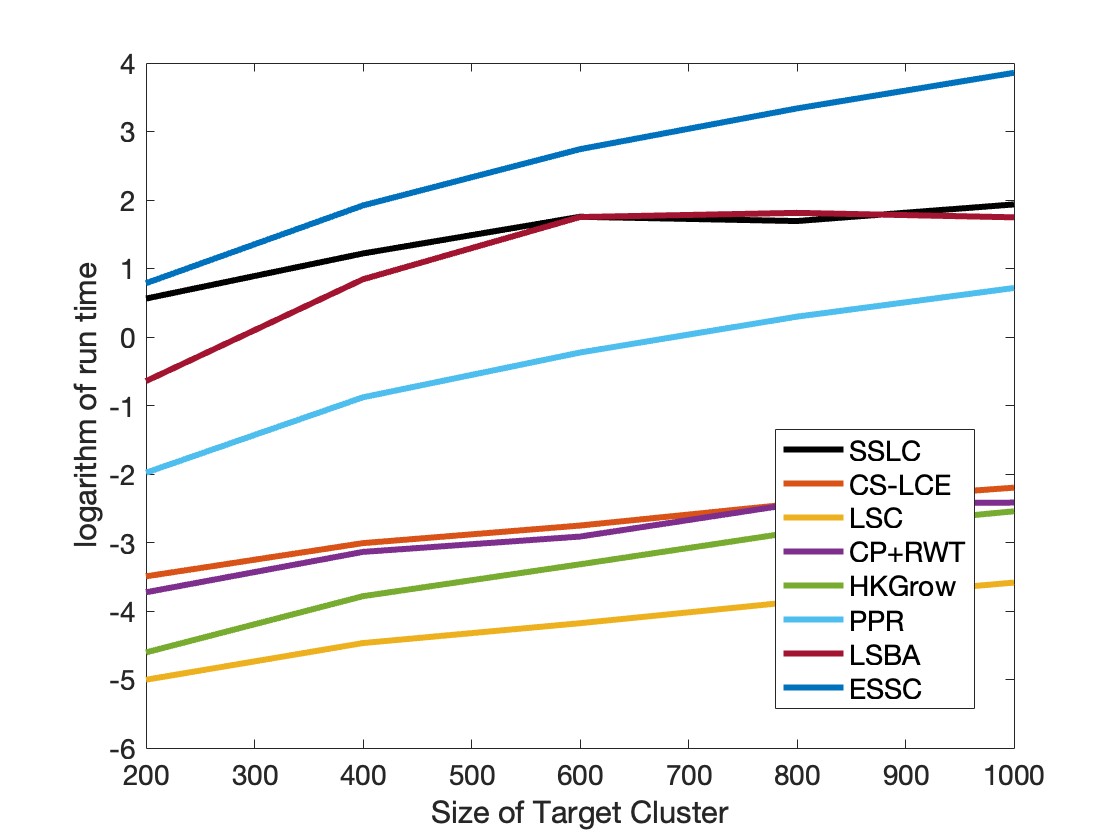
Figure 3: Jaccard Index (over 100 trials) and Logarithm of Running Time on Stochastic Block Model (First column: Jaccard index and run time of single cluster extraction for the symmetric case. Second column: Jaccard index and run time of all clusters extraction for the symmetric case. Third column: Jaccard index and run time of dominated cluster extraction for the nonsymmetric case)

To show the correctness of this procedure, the key step is to check that whenever a node $v$ being added to $\Gamma_{s}$ based on the large overlap criterion, it satisfies $v\in C_{s}$. The follow result establishes the correctness of Algorithm 1 and 2. We provide its proof in Appendix F.

Theorem 1

Suppose $G$ satisfies Assumptions 1 - 3. Then when $n$ (the size of $G$) gets large, for each $s=1,\cdots,k$, we have

$$|\tilde{C}_{s}\cap C^{\#}|=\begin{cases}>(1-o(1))|C^{\#}|&\text{if}\text{ }v\in C_{s},\\ \leq o(|C^{\#}|)&\text{otherwise}\\ \end{cases}$$

Remark 4

One may think that we can simply add more nodes into $\Gamma_{s}$ based on the probability of each node being visited in the random walk step of LCE. However, it does not work well as the nodes being picked in this way are not random in general, they are more towards the “center” of each cluster, which has high probability. Therefore, if using those more centered nodes as seeds, it has a higher chance of extracting the wrong node along the perimeter.

3.2.2 Unsupervised Local Clustering

For the unsupervised case, we do not have any seeds available nor the information about the number of clusters, therefore we do not have an “anchored” cluster (such as the blue circle in the semi-supervised case). In this case, we can check its overlap with the local cluster obtained from any newly sampled node. One can randomly sample and build a local cluster from the sampled node every time. After a certain number of iterations, the nodes from the same underlying cluster will more likely to be clustered together. Let us illustrate the idea of unsupervised local clustering in Figure 2. We summarize its procedure in Algorithm 3.

1. Given a graph $G$, in each iteration, we randomly sample a node and find its local cluster via LCE (as shown in the top row of Figure 2).

2. Based on the found local cluster, build the co-membership matrix in such a way that it outputs $1$ in the location $(i,j)$ when both $i,j$ are contained in that found cluster, and outputs $0$ otherwise.

3. Aggregate the clustering results from all iteration into a co-membership matrix $M$ (roughly speaking, each entry $M_{i,j}$ represents the probability of a pair of nodes being clustered into the same local cluster). The values in each block of matrix $M$ will asymptotically converge to the same value, as the iteration number goes up (as shown in the bottom row of Figure 2).

4. Randomly sample a node $i$, and use a prescribed cutoff number $\delta$ to select all the nodes $u$ such that $M_{i,j}>\delta$ and assign those $j$’s as one of the clusters $C^{\#}$.

5. Delete the subgraph generated by $C^{\#}$ from the original graph $G$. Then keep iterating until the prescribed maximum number of clusters is reached or the remaining size of the graph is too small.

Table 1: Average accuracy and standard deviation on FashionMNIST (over 30 trials)

# Labels per class	0	1	2	3	4	5
Laplace Learning	-	18.4 (7.3)	32.5 (8.2)	44.0 (8.6)	52.2 (6.2)	57.9 (6.7)
Nearest Neighbor	-	44.5 (4.2)	50.8 (3.5)	54.6 (3.0)	56.6 (2.5)	58.3 (2.4)
Random Walk	-	49.0 (4.4)	55.6 (3.8)	59.4 (3.0)	61.6 (2.5)	63.4 (2.5)
VolumeMBO	-	54.7 (5.2)	61.7 (4.4)	66.1 (3.3)	68.5 (2.8)	70.1 (2.8)
WNLL	-	44.6 (7.1)	59.1 (4.7)	64.7 (3.5)	67.4 (3.3)	70.0 (2.8)
$p$-Laplace	-	54.6 (4.0)	57.4 (3.8)	65.4 (2.8)	68.0 (2.9)	68.4 (0.5)
PoissonMBO	-	62.0 (5.7)	67.2 (4.8)	70.4 (2.9)	72.1 (2.5)	73.1 (2.7)
SSLC/USLC	61.6 (6.2)	65.8 (4.1)	69.1 (3.2)	74.3 (2.3)	77.2 (2.6)	78.7 (2.3)

Table 2: Average accuracy and standard deviation on CIFAR-10 (over 30 trials)

# Labels per class	0	1	2	3	4	5
Laplace Learning	-	10.4 (1.3)	11.0 (2.1)	11.6 (2.7)	12.9 (3.9)	14.1 (5.0)
Nearest Neighbor	-	31.4 (4.2)	35.3 (3.9)	37.3 (2.8)	39.0 (2.6)	40.3 (2.3)
Random Walk	-	36.4 (4.9)	42.0 (4.4)	45.1 (3.3)	47.5 (2.9)	49.0 (2.6)
VolumeMBO	-	38.0 (7.2)	46.4 (7.2)	50.1 (5.7)	53.3 (4.4)	55.3 (3.8)
WNLL	-	16.6 (5.2)	26.2 (6.8)	33.2 (7.0)	39.0 (6.2)	44.0 (5.5)
$p$-Laplace	-	26.0 (6.7)	35.0 (5.4)	42.1 (3.1)	48.1 (2.6)	49.7 (3.8)
PoissonMBO	-	41.8 (6.5)	50.2 (6.0)	53.5 (4.4)	56.5 (3.5)	57.9 (3.2)
SSLC/USLC	48.2 (6.1)	51.2 (5.2)	57.1 (4.9)	59.7 (4.7)	61.3 (3.4)	63.5 (2.7)

As it is the case for most local clustering methods, Algorithm 2 and Algorithm 3 also are applicable if there are outlier nodes, i.e., nodes which do not belong to any underlying clusters, presented in the graph. In such case, we can extract all the clusters and then the remaining parts will be the outlier nodes. We demonstrate the effectiveness for this case in the last part of experimental section.

To show the correctness of this procedure, we show that $M_{i,j}$, the probability of a pair of nodes coming from the same underlying cluster, is significantly different from the probability of a pair of nodes coming from two different underlying clusters. We establish the following results and we provide proofs in Appendix F.

Lemma 3

Suppose $G$ satisfies Assumptions 1 - 3. Let $v$ be any sampled node with $v\in C_{s}$ for some $s\geq 1$. Then, as $n$ gets large, the cardinality of the set $S:=\{i\in C_{r}:{\rm comembership}(\mathbf{1}_{C^{\#}})_{v,i}={\rm comembership}(\mathbf{1}_{C_{s}})_{v,i}\}$ satisfies

$$\begin{array}[]{rll}|S|&\geq\;(1-o(1))n_{\min},&\text{if}\text{ }\text{ }r=s,\\ |S|&\leq\;o(n_{\min}),&\text{otherwise.}\\ \end{array}$$

Lemma 4

Suppose $G$ satisfies Assumptions 1 - 3. Then, as $n$ gets large, the co-membership matrix $M$ obtained from Algorithm 3 has a clear block diagonal form (after permutation) as $L\to\infty$. More precisely, the entries in $M$ satisfy

$$\begin{cases}M_{i,j}\geq(1-o(1))\frac{n_{\min}}{n},&\text{for any}\text{ }i=j,\\ M_{i,j}\geq(1-o(1))\frac{n_{\min}^{2}}{nn_{s}},&\text{for}\text{ }i,j\in C_{s},i\neq j,s\geq 1,\\ M_{i,j}\leq o\left(\frac{4n^{2}_{\min}(1-o(1))}{n^{2}}\right),&\text{otherwise.}\end{cases}$$

Theorem 2

Suppose the assumptions in Theorem 4 hold. For any $v\in C_{s},s\geq 1$, there exists some $\delta\in(0,1)$ and $C_{s}^{\#}=\{i:M_{v,i}>\delta\}$ such that $C_{s}^{\#}=C_{s}$. Consequently, Algorithm 3 assigns all nodes into their clusters correctly.

Table 3: Average accuracy and standard deviation of SSLC/USLC by adding $10\%$ number of outliers (over 30 trials)

# Labels Per Class	0	1	2	3	4	5
FashionMNIST	55.6 (6.7)	60.4 (6.2)	65.6 (5.9)	69.9 (4.7)	73.5 (4.0)	74.8 (3.9)
CIFAR-10	45.1 (7.9)	47.3 (7.3)	51.6 (7.0)	55.3 (5.9)	58.1 (5.4)	60.1 (4.7)

4 Experiments

We evaluate the performance of SSLC and USLC on both synthetic and real datasets, with a particular focus on clustering in the low-label rates regime, which is the most challenging scenario for many semi-supervised clustering methods. Additionally, we demonstrate the robustness of our methods by manually introducing outliers into the dataset and assessing their impact. All experiments can be run on a personal laptop, with each trial taking only a few seconds to minutes. We provide supplementary material to support our experimental results.

4.1 Synthetic Data

We first conduct two experiments under semi-supervised setting on stochastic block models with different cluster sizes and different connection probabilities. The first case is symmetric stochastic block model with three equal cluster size, the second case is general stochastic block model with three unequal clusters sizes. The parameters for generating data in both cases are included in Appendix C.

For the symmetric case, we focus on both a single cluster extraction and all clusters extraction. For the nonsymmetric case, we only focus on extracting the most dominant cluster, i.e., the cluster with the largest connection probability. We compare against several other local clustering algorithms such as CS-LCE or LCE (Shen et al., 2023), LSC (Lai and Shen, 2023), CP+RWT (Lai and Mckenzie, 2020), HKGrow (Kloster and Gleich, 2014), PPR (Andersen et al., 2006), ESSC (Wilson et al., 2014), LBSA (Shi et al., 2019). In all experiments for stochastic block model, the number of initial seeds is set to be 1. The results are shown in Figure 3.

We can see that, for symmetric model, the Jaccard indices in both single cluster extraction and all clusters extraction are similar, while the running time of all clusters extraction is more advantageous towards SSLC (see also Remark 3). It is also worthwhile to note that for nonsymmetric model, the Algorithm ESSC starts to fail when the number of nodes increases.

We further compare our algorithm against other compressive sensing based local clustering methods on a geometric dataset consisting of different shapes (three lines, three circles, three moons). We use one label per class, the clustering results are shown in Table 4. The 2D projection and more details of this dataset are provided in Appendix B. Note that traditional method such as spectral clustering often fails on these three shapes of point cloud.

Table 4: Average accuracy and standard deviation on geometric data (over 100 trials)

Datasets	3 Lines	3 Circles	3 Moons
Spectral Clustering	-	-	-
CP+RWT	82.1 (9.1)	96.1 (5.1)	85.4 (1.3)
LSC	89.0 (5.5)	96.2 (3.7)	85.3 (1.9)
LCE	92.4 (8.1)	97.6 (4.7)	96.8 (0.9)
SSLC	94.8 (7.2)	98.2 (4.1)	97.3 (1.2)

4.2 Real Data

For real datasets, we focus on clustering in the low-label rates regime on FashionMNIST (Xiao et al., 2017), and CIFAR-10 (Krizhevsky et al., 2009). To apply graph-based clustering algorithms on images, we first construct an auxiliary graph, e.g., a KNN-graph. We compute the pairwise distance from Gaussian kernel based on the Euclidean distance of the latent features with some scaling factors. Similar constructions have also appeared among others (Zelnik-Manor and Perona, 2004; Jacobs et al., 2018; Calder et al., 2020). More detailed of construction is provided in Appendix C.

Figure 4: Affinity matrix of FashionMNIST after adding the outlier images (the last block consists of $10\%$ outliers compared to the size of original dataset)

We compare against other modern semi-supervised clustering algorithms such as Poisson learning and PoissonMBO (Calder et al., 2020) Laplace learning (Zhu et al., 2003), lazy random walks (Zhou and Scholkopf, 2004; Zhou et al., 2004a), weighted nonlocal laplacian (WNLL) (Shi et al., 2017), volume constrained MBO (Jacobs et al., 2018), and $p$-Laplace learning (Flores et al., 2022). We also evaluate a nearest neighbor classifier, which assigns the label of the nearest labeled vertex based on the graph geodesic distance. The results are summarized in Table 1 and 2. Note that other methods can only handle the semi-supervised case, i.e., the number of label(s) per class is at least one.

To further demonstrate the robustness of our methods against outliers in the graph, we manually add some images consisting of random noise as outliers into the datasets. Specifically, we add the number of outliers equal to $10\%$ of the original dataset size. Each outlier image is generated by setting its pixel values equal to the standard Gaussian random noise. As shown in Figure 4, the last block consists entirely of outliers, exhibiting no community structure, while other blocks do. Such case is also called tight clustering in the literature (Tseng and Wong, 2005; Deng et al., 2024). Table 3 further confirms that the performance of our proposed methods remains largely unaffected in the presence of these outliers.

5 Conclusion and Discussion

We proposed a unified framework for extracting local clusters in both semi-supervised and unsupervised settings with theoretical guarantees. The methods require minimal label information in the semi-supervised case and no label information in the unsupervised case, achieving state-of-the-art results. Notably, the methods are very effective particularly in the low-label rates regime, and remain robust when outliers are presented in the data. One limitation of this work is that when the label rates are not extremely low, the performance of proposed method in the semi-supervised case do not exhibit advantages over other methods.

Appendix A Notations

Table 5: Table of Notations

Symbols	Interpretations
$G$	general graph of interest
$E$	set of edges of graph G
$V$	set of nodes in $G$ (size denoted by $n$)
$C_{s}$	each underlying true cluster
$C_{s}^{\#}$	each extracted cluster from algorithm
$\Gamma_{s}$	set of Seeds for each cluster
$U$	removal set from $V$ in Algorithm 4
$G^{in}$	subgraph of $G$ on $V$ with edge set $E^{in}$
$G^{out}$	subgraph of $G$ on $V$ with edge set $E^{out}$
$E^{in}$	subset of $E$ which consists only intra-connection edges
$E^{out}$	the complement of $E^{in}$ within $E$
$A\text{ }(A^{in})$	adjacency matrix of $G\text{ }(G^{in})$
$L\text{ }(L^{in})$	random walk Laplacian matrix of $G\text{ }(G^{in})$
$L_{C}\text{ }(L^{in}_{C})$	submatrix of $L\text{ }(L^{in})$ with column indices $C\subset V$
$\ell_{i}\text{ }(\ell_{i}^{in})$	$i$-th column of $L\text{ }(L^{in})$
$L^{in}_{\Omega}$	submatrix of $L^{in}$ with column indices $\Omega\subset V$
$|M|$	entrywised absolute value operation on matrix $M$
$\|M\|_{2}$	$\|\cdot\|_{2}$ norm of matrix $M$
$|\mathbf{v}|$	entrywised absolute value operation on vector $\mathbf{v}$
$\|\mathbf{v}\|_{2}$	$\|\cdot\|_{2}$ norm of vector $\mathbf{v}$.
$\mathbf{1}_{C}$	indicator vector on subset $C\subset V$
$\triangle$	set symmetric difference
$\mathcal{L}_{s}(\mathbf{v})$	$\{i\in[n]:\text{$v_{i}$ among $s$ largest-in-magnitude entries in $\mathbf{v}$}\}$

Appendix B Geometric Dataset

B.1 Geometric Dataset

Three Lines

We generate three parallel lines in the $x$-$y$ plane defined by:

• Line 1: $y=0$ with $x\in[0,6]$

• Line 2: $y=1$ with $x\in[0,6]$

• Line 3: $y=2$ with $x\in[0,6]$

For each line, we sample 1,200 points uniformly at random. The embedding into $\mathbb{R}^{100}$ is performed as:

1. Zero-padding: $(x,y)\mapsto(x,y,0,\ldots,0)\in\mathbb{R}^{100}$

2. Noise addition: Each coordinate $z_{i}$ is perturbed as $z_{i}\leftarrow z_{i}+\epsilon_{i}$ where $\epsilon_{i}\sim\mathcal{N}(0,0.15)$

Three Circles

We construct three concentric circles with:

• Circle 1: Radius $r=1.0$ (500 points)

• Circle 2: Radius $r=2.4$ (1,200 points)

• Circle 3: Radius $r=3.8$ (1,900 points)

Points are sampled uniformly along each circle, totaling 3,600 points. The $\mathbb{R}^{100}$ embedding follows the same zero-padding and noise injection procedure as above.

Three Moons

Three semicircular clusters are generated with:

• Moon 1: Upper semicircle, radius $1.0$, centered at $(0,0)$ (1,200 points)

• Moon 2: Lower semicircle, radius $1.5$, centered at $(1.5,0.4)$ (1,200 points)

• Moon 3: Upper semicircle, radius $1.0$, centered at $(3,0)$ (1,200 points)

Each dataset uses identical embedding:

$$(x,y)\mapsto(x,y,0,\ldots,0)+\boldsymbol{\epsilon},\quad\boldsymbol{\epsilon}\sim\mathcal{N}(\mathbf{0},0.15^{2}\mathbf{I}_{100})$$

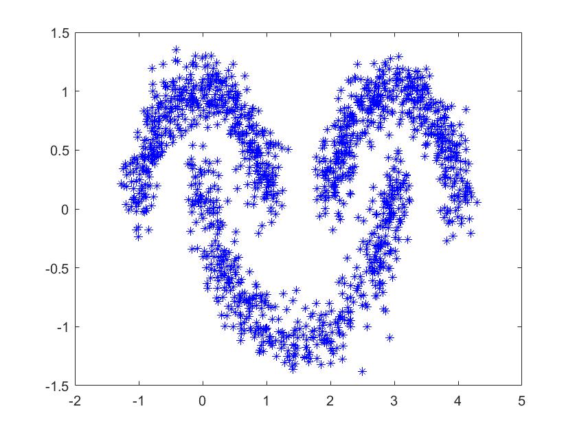
Figure 5: 2D Visulization of Geometric Dataset

Appendix C Implementation Details

C.1 Constructing KNN Graphs

Let $\mathbf{x}_{i}\in\mathbb{R}^{n}$ be the vectorization of an image or the feature extracted from an image, we define the following affinity matrix of the $K$-NN auxiliary graph based on Gaussian kernel:

$$A_{ij}=\begin{cases}e^{-\|\mathbf{x}_{i}-\mathbf{x}_{j}\|^{2}/\sigma_{i}\sigma_{j}}&\text{if}\quad\mathbf{x}_{j}\in NN(\mathbf{x}_{i},K),\\ 0&\text{otherwise}.\end{cases}$$

Note that similar construction has also appeared among others [Zelnik-Manor and Perona, 2004, Jacobs et al., 2018, Calder et al., 2020]. To construct high-quality graphs, we trained autoencoders to extract key features from the image data, we adopt the same parameters as [Calder et al., 2020] for training autoencoders to obtain these features.

The notation $NN(\mathbf{x}_{i},K)$ indicates the set of $K$-nearest neighbours of $\mathbf{x}_{i}$, and $\sigma_{i}:=\|\mathbf{x}_{i}-\mathbf{x}^{(r)}_{i}\|$ where $\mathbf{x}^{(r)}_{i}$ is the $r$-th closest point of $\mathbf{x}_{i}$. Note that the above $A_{ij}$ is not necessary symmetric, so we consider $\tilde{A}_{ij}=A^{T}A$ for symmetrization. Alternatively, one may also want to consider $\tilde{A}=\max\{A_{ij},A_{ji}\}$ or $\tilde{A}=(A_{ij}+A_{ji})/2$. We use $\tilde{A}$ as the input adjacency matrix for our algorithms. In our experiments, the local scaling parameters are chosen to be $K=15$, $r=10$ for all three real image datasets.

C.2 Parameters of Synthetic Data Generating and Algorithms

In all implementations where the LCE are applied, we sampled the seeds $\Gamma_{i}$ uniformly from each $C_{i}$ for all the implementations. We fix the rejection parameter $R=0.1$, the random walk depth $t=3$, random walk threshold parameter $\epsilon=0.8$, and the removal set parameter $\gamma=0.2$ for all experiments.

For synthetic data, the symmetric stochastic block model consists of three equal size clusters of $n_{1}=200,400,600,800,1000$ with connection probability $p=5\log(3n_{1})/(3n_{1})$ and $q=\log(3n_{1})/(3n_{1})$. The general stochastic block model consists of clusters’ sizes as $\mathbf{n}=(n_{1},2n_{1},5n_{1})$ where $n_{1}$ is chosen from $200,400,600,800,1000$, and the connection probability has the matrix form

$$P=[P_{11},P_{12},P_{13};P_{21},P_{22},P_{23};P_{31},P_{32},P_{33}]$$

with $P_{11}=\log^{2}(8n_{1})/(6n_{1})$, $P_{22}=\log^{2}(8n_{1})/(12n_{1})$, $P_{33}=\log^{2}(8n_{1})/(30n_{1})$, $P_{12}=P_{21}=P_{13}=P_{31}=P_{23}=P_{32}=\log(8n_{1})/(6n_{1})$. In the implementation of SSLC on synthetic data, we choose the iteration number $L=60$ in the symmetric case and $L=90$ in the nonsymmetric case.

In the implementation of SSLC on FashionMNIST and CIFAR-10 (both with and w/o outliers), we choose the iteration number to be $L=50k$ where $k$ is the number of seeds, i.e., $k=1,2,3,4,5$. In the implementation of USLC on FashionMNIST and CIFAR-10 (both with and w/o outliers), we choose the iteration number to be $L=1000$, and we set $\delta=0.01$ for FashionMNIST and $\delta=0.005$ for CIFAR-10.

Appendix D Background on Compressive Sensing and Sparse Solution Technique

The concept of compressive sensing (also called compressed sensing or sparse sampling) emerged from fundamental challenges in signal acquisition and efficient data compression. At its core, it addresses the inverse problem of recovering a sparse (or compressible) signal from a small number of noisy linear measurements:

$$\min_{\mathbf{x}\in\mathbb{R}^{n}}\|\mathbf{x}\|_{0}\quad s.t.\quad\|\Phi\mathbf{x}-\mathbf{y}\|_{2}\leq\epsilon,$$ (6)

where $\Phi\in\mathbb{R}^{m\times n}$ is called sensing matrix (usually underdetermined), $\mathbf{y}\in\mathbb{R}^{n}$ is called measurement vector, and the “zero quasi-norm” $\|\cdot\|_{0}$ counts the number of nonzero components in a vector. Among the key contributors, Donoho [Donoho, 2006] and Candès, Romberg and Tao [Candès et al., 2006] are widely credited with being the first to explicitly introduce this concept and make it popular. Since then, two families of approaches such as thresholding type of algorithms [Blumensath and Davies, 2009] and greedy type of algorithms [Tropp, 2004, Feng et al., 2021, Lai and Shen, 2020] have been developed based on the idea of compressive sensing. One particular type of greedy algorithms that has garnered our attention is the subspace pursuit [Dai and Milenkovic, 2009].

One of the reasons behind the remarkable usefulness of compressive sensing lies in its robustness against errors, including both additive and multiplicative types. More precisely, suppose we know $\mathbf{y}=\Phi\mathbf{x}^{*}$ where $\mathbf{y}$ is the exact measurement of the acquired signal and $\Phi$ is the exact measurement of the sensing matrix. However, we may only be able to access to the noisy version $\tilde{\mathbf{y}}=\mathbf{y}+\Delta\mathbf{y}$ and $\tilde{\Phi}=\Phi+\Delta\Phi$. In such case, we can still approximate the solution $\mathbf{x}^{*}$ well from the noisy measurements $\tilde{\mathbf{y}}$ and $\tilde{\Phi}$, as explained in the work of [Herman and Strohmer, 2010]. A unified framework of lifted $\ell_{1}$ form is explored in [Rahimi et al., 2024]. For Subspace Pursuit algorithm, we have the following result in [Li, 2016].

Lemma 5

Let $\mathbf{x}^{*}$, $\mathbf{y}$, $\tilde{y}$, $\Phi$, $\tilde{\Phi}$ be as defined above, and for any $t\in[n]$, let $\delta_{s}:=\delta_{s}(\tilde{\Phi})$. Suppose that $\|\mathbf{x}^{*}\|_{0}\leq s$. Define the following constants:

$$\epsilon_{\mathbf{y}}:=\|\mathbf{\Delta\mathbf{y}}\|_{2}/\|\mathbf{y}\|_{2}\quad\text{and}\quad\epsilon_{\Phi}^{s}:=\|\Delta\Phi\|_{2}^{(s)}/\|\Phi\|_{2}^{(s)}$$

where $\|M\|_{2}^{(s)}:=\max\{\|M_{S}\|_{2}:S\subset[n],\#(S)=s\}$ for any matrix $M$. Define further:

$$\rho:=\frac{\sqrt{2\delta_{3s}^{2}(1+\delta_{3s}^{2})}}{1-\delta_{3s}^{2}}\quad\text{and}\quad\tau:=\frac{(\sqrt{2}+2)\delta_{3s}}{\sqrt{1-\delta_{3s}^{2}}}(1-\delta_{3s})(1-\rho)+\frac{2\sqrt{2}+1}{(1-\delta_{3s})(1-\rho)}.$$

Assume that $\delta_{3s}<0.4859$ and let $\mathbf{x}^{(m)}$ be the output of Algorithm 4 after $m$ iterations. Then:

$$\frac{\|\mathbf{x}^{*}-\mathbf{x}^{(m)}\|_{2}}{\|\mathbf{x}^{*}\|_{2}}\leq\rho^{m}+\tau\frac{\sqrt{1+\delta_{s}}}{1-\epsilon^{s}_{\Phi}}(\epsilon^{s}_{\Phi}+\epsilon_{\mathbf{y}}).$$

Appendix E Local Cluster Extraction (LCE)

Algorithm 4 Compressive Sensing of Local Cluster Extraction (CS-LCE or LCE [Shen et al., 2023])

0: Adjacency matrix $A$ of an underlying graph $G$, the seed(s) set $\Gamma\subset C$ for some target cluster $C$, a fixed number of random walk depth $t$

0: the output target cluster $C^{\#}$

1: Compute $L=I-D^{-1}A$, $P=AD^{-1}$, $\mathbf{v}^{0}=D\mathbf{1}_{\Gamma}$ and $\mathbf{v}^{(t)}=P^{t}\mathbf{v}^{(0)}$

2: Define $\Omega={\mathcal{L}}_{(1-\epsilon)\hat{n}}(\mathbf{v}^{(t)})$

3: Let $U$ be the set of column indices of $\gamma\cdot|\Omega|$ smallest components of the vector $|L_{\Omega}^{\top}|\cdot|L\mathbf{1}_{\Omega}|$.

4: Set $\mathbf{y}:=-\sum_{i\in V\setminus U}\ell_{i}=L\mathbf{1}_{V\setminus U}$. Let $\mathbf{x}^{\#}$ be the solution to

$$\operatorname*{arg\,min}_{\mathbf{x}\in\mathbb{R}^{|V|-|U|}}\{\|L_{V\setminus U}\mathbf{x}-\mathbf{y}\|_{2}:\|\mathbf{x}\|_{0}\leq\hat{n}_{1}-|U|\}$$ (7)

obtained by using $O(\log n)$ iterations of Subspace Pursuit Dai and Milenkovic [2009].

5: Let $C^{\#}=\{i:\mathbf{x}_{i}^{\#}>R\}$

Let $L^{in}$ be the matrix as in (1), then the true solution $\mathbf{x}^{*}$ which encodes the local cluster information is

$$\mathbf{x}^{*}:=\operatorname*{arg\,min}_{\mathbf{x}\in\mathbb{R}^{|V|-|U|}}\{\|L^{in}_{V\setminus U}\mathbf{x}-\mathbf{y}^{in}\|_{2}:\|\mathbf{x}\|_{0}\leq\hat{n}_{1}-|U|\}$$ (8)

where $\mathbf{y}^{in}=-\sum_{i\in V\setminus U}\ell^{in}_{i}=L^{in}\mathbf{1}_{V\setminus U}$. The following results are established in [Shen et al., 2023]. We refer the proofs to [Shen et al., 2023].

Theorem 3

Suppose $U\subset C_{1}$ and $0.1|C_{1}|<|U|<0.9|C_{1}|$. Then $\mathbf{x}^{*}=\mathbf{1}_{C_{1}\setminus U}\in\mathbb{R}^{|V|-|U|}$ is the unique solution to (8).

Lemma 6

Let $\Delta L:=L-L^{in}$. Suppose $U\subset C_{1}$ and $0.1|C_{1}|<|U|<0.9|C_{1}|$. Suppose further that $\|\Delta L\|_{2}=o(n^{-\frac{1}{2}})$ and $\delta_{3(|C_{1}|-|U|)}(L)=o(1)$. Then

$$\frac{\|\mathbf{x}^{\#}-\mathbf{x}^{*}\|_{2}}{\|\mathbf{x}^{*}\|_{2}}=o(1).$$ (9)

Theorem 4

Under the same assumption as Lemma 6. Then

$$\frac{|C_{1}\triangle C_{1}^{\#}|}{|C_{1}|}\leq o(1).$$ (10)

Appendix F Other Deferred Proofs

• Proof. [Proof of Lemma 2] First, we notice that $||L-L^{in}||_{2}=o(1)$, then

  $$\frac{||\Delta\mathbf{y}||_{2}}{||\mathbf{y}||_{2}}=\frac{||\mathbf{y}-\mathbf{y}^{in}||_{2}}{||\mathbf{y}||_{2}}=\frac{||(L-L^{in})\mathbf{1}_{V\setminus U}||_{2}}{||L\mathbf{1}_{V\setminus U}||_{2}}\leq\frac{o(1)\sqrt{n}}{||L\mathbf{1}_{U}||_{2}}.$$

  By Assumption 2,, the cluster $C_{1}$ is on the same order as the size of the graph $n$, hence $U\subset C_{1}$ is also on the same order as $n$. By Assumption 3, all the nodes asymptotically have the same degree, therefore $||L\mathbf{1}_{U}||_{2}=\Theta(||\mathbf{1}_{U}||_{2})=\Theta(\sqrt{n})$. Hence

  $$\frac{||\mathbf{y}-\mathbf{y}^{in}||_{2}}{||\mathbf{y}||_{2}}\leq\frac{o(1)\sqrt{n}}{\Theta(\sqrt{n})}=o(1).$$

  Therefore, the quantity $\epsilon_{\mathbf{y}}=o(1)$ in Lemma 5.

  With the same assumption $||L-L^{in}||_{2}=o(1)$, it is not hard to see that, if the singular values of $L$ decays at a reasonable rate, then by applying the eigenvalue interlacing theorem, we have $\epsilon_{\Phi}^{s}=o(1)$ as well (by letting $\Phi=L$ in Lemma 5 in Appendix D). With these, the second term on the right-hand-side of the inequality in Lemma 5 satisfies $\tau\frac{\sqrt{1+\delta_{s}}}{1-\epsilon^{s}_{\Phi}}(\epsilon^{s}_{\Phi}+\epsilon_{\mathbf{y}})\leq o(1)$.

  Furthermore, since $\mathbf{x}^{\#}$ is the output of Algorithm 4 after $m=O(\log n)$ iteration, we have $\rho^{m}=O\left((\delta_{3(|C_{1}|-|U|)})^{\log n}\right)=o(1)$.

  Putting these together gives

  $$\frac{||\mathbf{x}^{\#}-\mathbf{x}^{*}||_{2}}{||\mathbf{x}^{*}||_{2}}=o(1).$$

  $\Box$

• Proof. [Proof of Theorem 1] For any $s\geq 1$, let us case on whether $v\in C_{s}$ or not. If $v\in C_{s}$, then by Theorem 4, we have

  $$|C^{\#}\triangle(\tilde{C}_{s}\cap C^{\#})|\leq|C^{\#}\triangle(C_{s}\cap C^{\#})|+|(C_{s}\triangle\tilde{C}_{s})\cap C^{\#}|\leq o(|C^{\#}|)+o(|C^{\#}|)=o(|C^{\#}|).$$

  Therefore, $|\tilde{C}_{s}\cap C^{\#}|\geq|C^{\#}|-o(|C^{\#}|)=(1-o(1))|C^{\#}|$.

  If $v\in C_{t},t\neq s$, then $|C_{s}\cap C^{\#}|\leq o(|C^{\#}|)$. We have

  $$|C^{\#}\triangle(\tilde{C}_{s}\cap C^{\#})|\geq|C^{\#}\triangle(C_{s}\cap C^{\#})|-|(C_{s}\triangle\tilde{C}_{s})\cap C^{\#}|\geq|C^{\#}|-o(|C^{\#}|)-o(|C^{\#}|)=|C^{\#}|-o(|C^{\#}|).$$

  Therefore, $|\tilde{C}_{s}\cap C^{\#}|\leq|C^{\#}|-(|C^{\#}|-o(|C^{\#}|))=o(|C^{\#}|)$.

  $\Box$

• Proof. [Proof of Lemma 3] By Theorem 4, we have $|C^{\#}\triangle(C_{s}\cap C^{\#})|\leq o(C^{\#})=o(n_{\min})$. Therefore,

  $$|C^{\#}\triangle C_{s}|=|C^{\#}\triangle(C_{s}\cap C^{\#})|+|C_{s}\setminus C^{\#}|\leq o(n_{\min})+n_{s}-n_{\min}.$$

  Hence

  $$\left|\{i\in C_{s}:{\rm comembership}(\mathbf{1}_{C^{\#}})_{v,i}\neq{\rm comembership}(\mathbf{1}_{C_{s}})_{v,i}\}\right| =|(C^{\#}\triangle C_{s})\cap C_{s}|\leq|C^{\#}\triangle C_{s}|$$

  $$\leq o(n_{\min})+n_{s}-n_{\min}.$$

  So we conclude

  $$\left|\{i\in C_{s}:{\rm comembership}(\mathbf{1}_{C^{\#}})_{v,i}={\rm comembership}(\mathbf{1}_{C_{s}})_{v,i}\}\right| \geq n_{s}-(o(n_{\min})+n_{s}-n_{\min})$$

  $$=n_{\min}-o(n_{\min}).$$

  As $C_{s}\cap C_{t}=\emptyset$, we have $|C^{\#}\cap C_{t}|\leq o(n_{min})$. Therefore,

  $$\left|\{i\in C_{t}:{\rm comembership}(\mathbf{1}_{C^{\#}})_{v,i}={\rm comembership}(\mathbf{1}_{C_{t}})_{v,i}\}\right|\leq o(n_{\min}).$$

  $\Box$

• Proof. [Proof of Lemma 4] By Lemma 3, we have the following estimates for the entries in the comembership matrix $M$ asymptotically.

  For any $i=j\in C_{s}$, some $s\geq 1$, the entries in $M$ satisfies

  $$M_{i,i}\geq\frac{n_{s}}{n}\cdot\frac{(1-o(1))n_{\min}}{n_{s}}=(1-o(1))\frac{n_{\min}}{n}.$$

  For any distinct $i,j\in C_{s}$, $s\geq 1$, the entries in $M$ satisfies

  $$M_{i,j}\geq\frac{n_{s}}{n}\cdot\left(\frac{(1-o(1))n_{\min}}{n_{s}}\right)^{2}=(1-o(1))\frac{n_{\min}^{2}}{nn_{s}}.$$

  For any distinct $i,j$ such that $i\in C_{s}$, $j\in C_{t}$, $s\neq t$, the entries in $M$ satisfies

  $$M_{i,j} \leq\frac{n_{s}}{n}\cdot\frac{(1-o(1))n_{\min}}{n_{s}}\cdot\frac{o(n_{\min})}{n-n_{s}}+\frac{n_{t}}{n-n_{t}}\cdot\frac{(1-o(1))n_{\min}}{n_{t}}\cdot\frac{o(n_{\min})}{n}$$

  $$\leq\frac{2n^{2}_{\min}(1-o(1))\cdot o(1)}{n^{2}}+\frac{2n^{2}_{\min}(1-o(1))\cdot o(1)}{n^{2}}$$

  $$=o\left(\frac{4n^{2}_{\min}(1-o(1))}{n^{2}}\right).$$

  $\Box$

• Proof. [Proof of Theorem 2] By direct computation, we can choose $\delta=(\frac{n_{min}}{n})^{2}$ such that

  $$\frac{n_{\min}}{n}(1-o(1))>\delta>o\left(\frac{4n^{2}_{\min}(1-o(1))}{n^{2}}\right)$$

  and

  $$\frac{n_{\min}^{2}}{nn_{s}}(1-o(1))>\delta>o\left(\frac{4n^{2}_{\min}(1-o(1))}{n^{2}}\right).$$

  Hence, for any $i\in C_{s}$ satisfies $M_{v,i}>\delta$, and any $i\in C_{t},t\neq s$, satisfies $M_{v,i}<\delta$. So we conclude $C_{s}^{\#}=C_{s}$. $\Box$

Remark 5

Note that All the statements in Theorem 1 and 2, Lemma 2, 3 and 4, are asymptotic statements, and the little $o$ notation is with respect to when $n\to\infty$.

References

- Andersen et al. [2006] Reid Andersen, Fan Chung, and Kevin Lang. Local graph partitioning using pagerank vectors. In IEEE Symposium on Foundations of Computer Science, pages 475–486. IEEE, 2006.
- Andersen et al. [2016] Reid Andersen, Shayan Oveis Gharan, Yuval Peres, and Luca Trevisan. Almost optimal local graph clustering using evolving sets. Journal of the ACM (JACM), 63(2):1–31, 2016. doi: 10.1145/2856033. Article No. 15.
- Ando and Zhang [2007] R. K. Ando and T. Zhang. Learning on graph with laplacian regularization. In Advances in Neural Information Processing Systems (NeurIPS), pages 25–32. MIT Press, 2007.
- Blumensath and Davies [2009] Thomas Blumensath and Mike E. Davies. Iterative hard thresholding for compressed sensing. Applied and Computational Harmonic Analysis, 27(3):265–274, 2009.
- Calder and Slepcev [2019] J. Calder and D. Slepcev. Properly-weighted graph laplacian for semi-supervised learning. Applied Mathematics & Optimization, Dec 2019.
- Calder et al. [2020] Jeff Calder, Brendan Cook, Matthew Thorpe, and Dejan Slepcev. Poisson learning: Graph based semi-supervised learning at very low label rates. In Proceedings of the International Conference on Machine Learning (ICML), pages 1306–1316. PMLR, 2020.
- Candès et al. [2006] Emmanuel J. Candès, Justin Romberg, and Terence Tao. Robust uncertainty principles: Exact signal reconstruction from highly incomplete frequency information. IEEE Transactions on Information Theory, 52(2):489–509, 2006.
- Dai and Milenkovic [2009] Wei Dai and Olgica Milenkovic. Subspace pursuit for compressive sensing signal reconstruction. IEEE Transactions on Information Theory, 55(5):2230–2249, May 2009.
- Deng et al. [2024] Jiayi Deng, Xiaodong Yang, Jun Yu, Jun Liu, Zhaiming Shen, Danyang Huang, and Huimin Cheng. Network tight community detection. In Forty-first International Conference on Machine Learning, 2024.
- Donoho [2006] David L. Donoho. Compressed sensing. IEEE Transactions on Information Theory, 52(4):1289–1306, 2006.
- El Alaoui et al. [2016] A. El Alaoui, X. Cheng, A. Ramdas, M. J. Wainwright, and M. I. Jordan. Asymptotic behavior of -based laplacian regularization in semi-supervised learning. In Conference on Learning Theory (COLT), pages 879–906, 2016.
- Ester et al. [1996] Martin Ester, Hans-Peter Kriegel, Jörg Sander, and Xiaowei Xu. A density-based algorithm for discovering clusters in large spatial databases with noise. In Proceedings of the 2nd International Conference on Knowledge Discovery and Data Mining (KDD), pages 226–231, 1996.
- Feng et al. [2021] Renzhong Feng, Aitong Huang, Ming-Jun Lai, and Zhaiming Shen. Reconstruction of sparse polynomials via quasi-orthogonal matching pursuit method. Journal of Computational Mathematics, 2021.
- Flores et al. [2022] Mauricio Flores, Jeff Calder, and Gilad Lerman. Analysis and algorithms for -based semi-supervised learning on graphs. Applied and Computational Harmonic Analysis, 60:77–122, 2022.
- Fountoulakis et al. [2020] Kimon Fountoulakis, Di Wang, and Shenghao Yang. -norm flow diffusion for local graph clustering. In Proceedings of the International Conference on Machine Learning (ICML), pages 3222–3232, 2020.
- Hamel et al. [2024] Jackson Hamel, Ming-Jun Lai, Zhaiming Shen, and Ye Tian. Local clustering for lung cancer image classification via sparse solution technique. arXiv preprint arXiv:2407.08800, 2024.
- Herman and Strohmer [2010] Matthew A. Herman and Thomas Strohmer. General deviants: An analysis of perturbations in compressed sensing. IEEE Journal of Selected Topics in Signal Processing, 4(2):342–349, 2010.
- Jacobs et al. [2018] M. Jacobs, E. Merkurjev, and S. Esedoglu. Auction dynamics: A volume constrained mbo scheme. Journal of Computational Physics, 354:288–310, 2018.
- Kang et al. [2011] Sung Ha Kang, Berta Sandberg, and Andy M Yip. A regularized k-means and multiphase scale segmentation. Inverse Problems and Imaging, 5(2):407–429, 2011.
- Kang et al. [2014] Sung Ha Kang, Behrang Shafei, and Gabriele Steidl. Supervised and transductive multi-class segmentation using p-laplacians and rkhs methods. Journal of Visual Communication and Image Representation, 25(5):1136–1148, 2014.
- Kloster and Gleich [2014] Kyle Kloster and David F. Gleich. Heat kernel based community detection. In Proceedings of the 20th ACM SIGKDD International Conference on Knowledge Discovery and Data Mining, pages 1386–1395. ACM, 2014.
- Krizhevsky et al. [2009] Alex Krizhevsky, Geoffrey Hinton, et al. Learning multiple layers of features from tiny images, 2009.
- Lai and Mckenzie [2020] Ming-Jun Lai and Daniel Mckenzie. Compressive sensing for cut improvement and local clustering. SIAM Journal on Mathematics of Data Science, 2(2):368–395, 2020.
- Lai and Shen [2020] Ming-Jun Lai and Zhaiming Shen. A quasi-orthogonal matching pursuit algorithm for compressive sensing. arXiv preprint arXiv:2007.09534, 2020.
- Lai and Shen [2023] Ming-Jun Lai and Zhaiming Shen. A compressed sensing based least squares approach to semi-supervised local cluster extraction. Journal of Scientific Computing, 94(3):63, 2023.
- Lang and Rao [2004] Kevin Lang and Satish Rao. A flow-based method for improving the expansion or conductance of graph cuts. In Proceedings of the International Conference on Integer Programming and Combinatorial Optimization (IPCO), pages 325–337, 2004.
- Li [2016] Haifeng Li. Improved analysis of sp and cosamp under total perturbations. EURASIP Journal on Advances in Signal Processing, 2016:1–6, 2016.
- MacQueen [1967] J. MacQueen. Classification and analysis of multivariate observations. In Proceedings of the Fifth Berkeley Symposium on Mathematical Statistics and Probability, pages 281–297, 1967.
- Ng et al. [2001] Andrew Ng, Michael Jordan, and Yair Weiss. On spectral clustering: Analysis and an algorithm. In Advances in Neural Information Processing Systems (NeurIPS), volume 14, 2001.
- Nielsen [2016] Frank Nielsen. Hierarchical clustering. In Introduction to HPC with MPI for Data Science, pages 195–211. 2016.
- Rahimi et al. [2024] Yaghoub Rahimi, Sung Ha Kang, and Yifei Lou. A lifted framework for sparse recovery. Information and Inference: A Journal of the IMA, 13(1):iaad055, 2024.
- Shen [2024] Zhaiming Shen. Sparse Solution Technique in Semi-Supervised Local Clustering and High Dimensional Function Approximation. Ph.d. dissertation, University of Georgia, 2024.
- Shen et al. [2023] Zhaiming Shen, Ming-Jun Lai, and Sheng Li. Graph-based semi-supervised local clustering with few labeled nodes. In Proceedings of the International Joint Conference on Artificial Intelligence (IJCAI), pages 4190–4198, 2023.
- Shi et al. [2019] Pan Shi, Kun He, David Bindel, and John E. Hopcroft. Locally-biased spectral approximation for community detection. Knowledge-Based Systems, 164:459–472, 2019.
- Shi et al. [2017] Z. Shi, S. Osher, and W. Zhu. Weighted nonlocal laplacian on interpolation from sparse data. Journal of Scientific Computing, 73(2-3):1164–1177, 2017.
- Spielman and Teng [2013] Daniel A. Spielman and Shang-Hua Teng. A local clustering algorithm for massive graphs and its application to nearly linear time graph partitioning. SIAM Journal on Computing, 42(1):1–26, 2013. doi: 10.1137/110853996.
- Tropp [2004] Joel A. Tropp. Greed is good: Algorithmic results for sparse approximation. IEEE Transactions on Information Theory, 50:2231–2242, 2004.
- Tseng and Wong [2005] George C Tseng and Wing H Wong. Tight clustering: a resampling-based approach for identifying stable and tight patterns in data. Biometrics, 61(1):10–16, 2005.
- Veldt et al. [2019] Nate Veldt, Christine Klymko, and David F. Gleich. Flow-based local graph clustering with better seed set inclusion. In Proceedings of the SIAM International Conference on Data Mining (SDM), pages 378–386. SIAM, 2019.
- Von Luxburg [2007] Ulrike Von Luxburg. A tutorial on spectral clustering. Statistics and Computing, 17:395–416, 2007.
- Wilson et al. [2014] James D. Wilson, Simi Wang, Peter J. Mucha, Shankar Bhamidi, and Andrew B. Nobel. A testing based extraction algorithm for identifying significant communities in networks. The Annals of Applied Statistics, 8:1853–1891, 2014.
- Xiao et al. [2017] Han Xiao, Karim Rasul, and Roland Vollgraf. Fashion-mnist: A novel image dataset for benchmarking machine learning algorithms. arXiv preprint arXiv:1708.07747, 2017.
- Zelnik-Manor and Perona [2004] Lihi Zelnik-Manor and Pietro Perona. Self-tuning spectral clustering. In Advances in Neural Information Processing Systems (NeurIPS), volume 17, 2004.
- Zhou and Scholkopf [2004] D. Zhou and B. Scholkopf. Learning from labeled and unlabeled data using random walks. In Joint Pattern Recognition Symposium, pages 237–244. Springer, 2004.
- Zhou et al. [2004a] D. Zhou, O. Bousquet, T. N. Lal, J. Weston, and B. Scholkopf. Learning with local and global consistency. In Advances in Neural Information Processing Systems, pages 321–328. MIT Press, 2004a.
- Zhou et al. [2004b] D. Zhou, J. Weston, A. Gretton, O. Bousquet, and B. Scholkopf. Ranking on data manifolds. In Advances in Neural Information Processing Systems (NeurIPS), pages 169–176. MIT Press, 2004b.
- Zhou et al. [2005] D. Zhou, J. Huang, and B. Scholkopf. Learning from labeled and unlabeled data on a directed graph. In Proceedings of the 22nd International Conference on Machine Learning, pages 1036–1043. ACM, 2005.
- Zhou and Belkin [2011] X. Zhou and M. Belkin. Semi-supervised learning by higher order regularization. In Proceedings of the Fourteenth International Conference on Artificial Intelligence and Statistics (AISTATS), pages 892–900, 2011.
- Zhu and Ghahramani [2002] Xiaojin Zhu and Zoubin Ghahramani. Learning from labeled and unlabeled data with label propagation, 2002. ProQuest number: information to all users.
- Zhu et al. [2003] Xiaojin Zhu, Zoubin Ghahramani, and John D. Lafferty. Semi-supervised learning using gaussian fields and harmonic functions. In Proceedings of the 20th International Conference on Machine Learning (ICML-03), pages 912–919, 2003.