Asymptotic expansions for Legendre functions via differential equations having coalescing turning points

Abstract

Linear second-order linear ordinary differential equations equations of the form $d^{2}w/dz^{2}=\{u^{2}f(a,z)+g(z)\}w$ are considered for large values of the real parameter $u$, $z$ being a complex variable ranging over a bounded or unbounded complex domain $Z$, and $a_{0}\leq a\leq a_{1}<\infty$. It is assumed that $f(a,z)$ and $g(z)$ are analytic in the interior of $Z$. Furthermore, $f(a,z)$ has exactly two real simple zeros in $Z$ for $a>a_{0}$ that depend continuously on $a$, and coalesce into a double zero as $a\to a_{0}$. Uniform asymptotic expansions are derived for solutions of the equation which involve parabolic cylinder functions and their derivatives, along with certain slowly varying coefficient functions. The new results involve readily computable coefficients and explicit error bounds, and are then applied to provide new asymptotic expansions for the associated Legendre functions when both the degree $\nu$ and order $\mu$ are large.

34E05, 33C05, 34M60, 34E20

1 Introduction

We consider differential equations of the form

(1) $$\frac{d^{2}w}{dz^{2}}=\left\{u^{2}f(a,z)+g(z)\right\}w.$$

For $a_{0}<a\leq a_{1}<\infty$ we assume that $f(a,z)$ has two real simple zeros at $z=z_{1}$ and $z=z_{2}$, which depend continuously on $a$, where $z_{1}<z_{2}$, and $z_{1}\to z_{2}$ as $a\to a_{0}$. We assume $f(a,z)$ and $g(z)$ are analytic in a certain domain $Z$ except possibly at the boundary of the domain. The domain $Z$ contains the two turning points, and $f(a,z)$ has no other zeros in $Z$. In addition, $f(a,z)$ is assumed to be real for real $z=x\in Z$, and $f(a,z)<0$ in $(z_{1},z_{2})$. Both $f(a,z)$ and $g(z)$ may depend on $u$ since explicit error bounds are included in the Liouville-Green (LG) expansions that we employ. Note that under the above hypotheses $f(a,z)>0$ for real $z\in Z$ such that $z<z_{1}$ and $z>z_{2}$.

These LG expansions come from the standard transformation of the equation (1) (see [19, Chap. 10]), but in the form where asymptotic expansions appear in the argument of an exponential function [4], rather than as a product with an exponential [19, Chap. 10]. Now, from [4, Eq. (1.3)], define $\xi$ by

(2) $$\xi=\int_{z_{2}}^{z}\{f(a,t)\}^{1/2}dt.$$

The branches are such that $\xi\geq 0$ for $z\geq z_{2}$ and by continuity elsewhere in $Z$ having a cut along $(-\infty,z_{2}]$. This transforms (1) into the standard LG form

(3) $$\frac{d^{2}W}{d\xi^{2}}=\left\{u^{2}+\psi(a,z)\right\}W,$$

where $W=f^{1/4}w$ and

(4) $$\psi(a,z)=\frac{4f(a,z)f^{\prime\prime}(a,z)-5f^{\prime}(a,z)^{2}}{16f(a,z)^{3}}+\frac{g(z)}{f(a,z)}.$$

It is clear that this is not analytic at the turning points $z=z_{j}$ ($j=1,2$) since $f(a,z)$ vanishes at these points, and this is why LG expansions are not valid there.

Fifty years ago, in a significant paper on the asymptotic theory of linear differential equations, Olver [17] made a change of independent variable $\zeta$ and introduced a new parameter $\alpha$, to construct asymptotic solutions that are valid at the turning points. From Olver [17, Eq. (2.8)] $\zeta$ is defined implicitly by

(5) $$\frac{d\zeta}{dz}=\left(\frac{f(a,z)}{\zeta^{2}-\alpha^{2}}\right)^{1/2},$$

With $\hat{W}=\{(\zeta^{2}-\alpha^{2})/f\}^{1/4}w$ (5) transforms (1) into the form

(6) $$\frac{d^{2}\hat{W}}{d\zeta^{2}}=\left\{u^{2}\left(\zeta^{2}-\alpha^{2}\right)+\hat{\psi}(\alpha,\zeta)\right\}\hat{W},$$

where

(7) $$\hat{\psi}(\alpha,\zeta)=\frac{3\zeta^{2}+2\alpha^{2}}{4\left(\zeta^{2}-\alpha^{2}\right)^{2}}+\left(\zeta^{2}-\alpha^{2}\right)\psi(a,z).$$

Integration of (5) and referring to (2) yields the implicit equation for $\zeta$

(8) $$\xi=\int_{\alpha}^{\zeta}\left(t^{2}-\alpha^{2}\right)^{1/2}dt=\frac{1}{2}\zeta\left(\zeta^{2}-\alpha^{2}\right)^{1/2}\\ -\frac{1}{2}\alpha^{2}\ln\left\{\zeta+\left(\zeta^{2}-\alpha^{2}\right)^{1/2}\right\}+\frac{1}{2}\alpha^{2}\ln(\alpha).$$

Note that as $\zeta\to\infty$

(9) $$\xi=\frac{1}{2}\zeta^{2}-\frac{1}{4}\alpha^{2}\left\{2\ln\left(\frac{2\zeta}{\alpha}\right)+1\right\}+\mathcal{O}\left(\frac{1}{\zeta^{2}}\right).$$

In Eqs. 2 and 8 the lower integration limits were chosen so that $\zeta=\alpha$ ($\xi=0$) corresponds to $z=z_{2}$. We also want $\zeta=-\alpha$ to correspond to $z=z_{1}$, and from (8) this is achieved by defining $\alpha$ by

(10) $$\int_{z_{1}}^{z_{2}}\{-f(a,t)\}^{1/2}dt=\int_{-\alpha}^{\alpha}\left(\alpha^{2}-t^{2}\right)^{1/2}dt=\frac{1}{2}\alpha^{2}\pi,$$

and therefore we have, on evaluating the second integral,

(11) $$\alpha=\left\{\frac{2}{\pi}\int_{z_{1}}^{z_{2}}\{-f(a,t)\}^{1/2}dt\right\}^{1/2}.$$

With this choice of $\alpha$, $\zeta$ is an analytic function of $z$ at $z=z_{j}$ ($j=1,2$). Moreover, unlike $\psi(a,z)$, one can verify that $\hat{\psi}(\alpha,\zeta)$ is also analytic at $\zeta=\pm\alpha$ (equivalently at $z=z_{1}$ and $z=z_{2}$).

Olver [17] constructed solutions of (6) of the form

(12) $$\hat{W}\left(u,\alpha,\zeta\right)=Y(u,\alpha,\zeta)+\epsilon(u,\alpha,\zeta),$$

where $Y(u,\alpha,\zeta)$ satisfies the so-called comparison equation

(13) $$\frac{d^{2}Y}{d\zeta^{2}}=u^{2}\left(\zeta^{2}-\alpha^{2}\right)Y,$$

which can be expressed in terms of parabolic cylinder functions. One such solution is $U(-\frac{1}{2}u\alpha^{2},\sqrt{2u}\,\zeta)$, where $U(b,z)$ is a parabolic cylinder function which is a solution of Weber’s equation

(14) $$\frac{d^{2}U}{dz^{2}}=\left(\frac{1}{4}z^{2}+b^{2}\right)U.$$

It is an important solution of the equation since it is the unique one that is recessive at $z=+\infty$ (see [3, Sect. 12.2]). In particular, we have

(15) $$U(b,z)\sim z^{-b-\frac{1}{2}}e^{-\frac{1}{4}z^{2}}\quad\left(z\to\infty,\,|\arg(z)|\leq\tfrac{3}{4}\pi-\delta\right),$$

and also

(16) $$U^{\prime}(b,z)\sim-\tfrac{1}{2}z^{-b+\frac{1}{2}}e^{-\frac{1}{4}z^{2}}\quad\left(z\to\infty,\,|\arg(z)|\leq\tfrac{3}{4}\pi-\delta\right).$$

Olver obtained explicit bounds for the error term $\epsilon$ which proved, assuming that $f$ and $g$ are bounded for large $u$ if dependent on that parameter, that $\epsilon=\mathcal{O}(u^{-p}\ln(u))$ as $u\to\infty$ relative to the magnitude of $y$ except near the zeros of that function. Here $p=\tfrac{2}{3}$ or $p=1$ depending on the sign of $f$ in the interval $(z_{1},z_{2})$. The bounds hold uniformly in an interval that is possibly unbounded or contains a singularity at one or both of its end points. He also obtained similar approximations and error bounds for the derivatives of these solutions. He also considered $u^{2}<0$ and $\alpha^{2}<0$. Our results can readily be extended to these cases, but we do not pursue those here.

Note that if the turning points are bounded away from one another, expansions at each turning point could be constructed in terms of Airy functions, using the well-known theory found in [19, Chap. 11]. This results in simpler expansions, but the price paid is that the parameters are more restricted. The significance of Olver’s paper is that his approximations are uniformly valid with respect to $\alpha\in[0,A]$, and thus for the turning points bounded away from one another, as well as being allowed to coalesce into a double zero when $\alpha\to 0$ (equivalently $a\to a_{0}$). The latter situation translates into a larger permissible range for the second parameter.

In a follow up paper Olver applied the theory to Legendre functions in [16], and later to Whittaker functions [18]. We too will apply the new expansions of the present paper to Legendre functions in Section 5, which extend Olver’s one-term approximations valid for real argument to full expansions, and also that are valid for complex values of the argument. In our approach we do not consider the ODE (6), rather we use the LG transformed equation Eq. 3 only. However, the variable $\zeta$ given by Eqs. 2 and 8 still plays a central role in our analysis.

We obtain expansions involving $U(-\frac{1}{2}u\hat{\alpha}^{2},\sqrt{2u}\,\zeta)$ and its derivative (along with other parabolic cylinder functions), where $\hat{\alpha}$ is a prescribed constant that is close in value to $\alpha$ for large $u$, but not necessarily exactly the same as that given by Eq. 10. The other parabolic cylinder functions that we shall use are $U(-\frac{1}{2}u\hat{\alpha}^{2},-\sqrt{2u}\,\zeta)$ and $U(\frac{1}{2}u\hat{\alpha}^{2},\pm i\sqrt{2u}\,\zeta)$. All four are solutions of (13) with $\alpha$ replaced by $\hat{\alpha}$, and are significant because they are recessive at $\zeta=\pm\infty$ and $\zeta=\mp i\infty$, respectively.

We extend Olver’s general results in several ways. Our results are valid for complex values of the argument rather than just real ones, with asymptotic expansions constructed rather than just the leading term. The coefficients in our new expansions are readily computable. We mention that Olver also showed how to obtain asymptotic expansions, but these involved very complicated expressions for the coefficients, and were only shown to be valid in finite intervals, and not valid at singularities. On the other hand, our expansions are valid in unbounded domains, as well as at certain singularities of the equation. Our results are rigorously justified with explicit and relatively simple error bounds. We also asymptotically solve the connection problem, which has applications to eigenvalue problems in quantum mechanics [1].

Earlier investigations into the problem of linear second order differential equations having two turning points include those by Kazarinoff [10], Langer [11, 12], and McKelvey [14]. For other studies, see [9, 13, 15]. The results we develop here are significantly more general, and have applications to the asymptotic evaluation of various special functions, including Whittaker functions, prolate spheroidal wave functions, Bessel polynomials, and Laguerre polynomials. Physical applications include wave scattering problems for electric cylinders and prolate spheroids [10], and the eigenfunctions of an anharmonic oscillator problem in quantum mechanics [8].

The plan of this paper is as follows. In Section 2 we construct LG solutions to Eq. 1, as well as establishing important connection formulas between them. These expansions are not themselves valid at $z=z_{1}$ and $z=z_{2}$, but will be used to construct asymptotic solutions that are valid at these turning points. In Section 3 we obtain LG expansions for the parabolic cylinder functions, and these, along with the results of Section 2, are used in Section 4 to obtain our main result, namely expansions that are valid at the turning points, uniformly for $a_{0}\leq a\leq a_{1}$. In Section 5 apply our new theory to obtain uniform asymptotic expansions for the associated Legendre functions when both the degree $\nu$ and the order $\mu$ are large. Finally in Section 6 we illustrate the accuracy of our uniform expansions with some numerical results from Section 5 for two cases, where the turning points in question are both close and not close.

2 LG expansions for the general equation

Let points $z=x_{j}$ ($j=1,2,3,4$) in the $z$ plane correspond to $\zeta=i\infty$, $+\infty$, $-i\infty$, and $-\infty$, respectively. Since $\zeta$ is unbounded at these points, the corresponding $z$ points must also be unbounded, or at a finite point that is a singularity of (1). We assume that all four are boundary points of $Z$.

From Eqs. 2 and 8, and recalling that $f(a,z)>0$ for $z<z_{1}$ and $z>z_{2}$, the points $x_{2}$ and $x_{4}$ lie on the real axis with $-\infty\leq x_{4}<z_{1}\leq z_{2}<x_{2}\leq\infty$, and $x_{1}$ and $x_{3}$ lie in the upper and lower half-planes, respectively.

At any finite point(s) $z=x_{j}$ ($j\in\{1,2,3,4\}$), which are singularities, must have the properties:

(i) $f(a,z)$ has a pole of order $m>2$, and $g(z)$ is analytic or has a pole of order less than $\frac{1}{2}m+1$, or

(ii) $f(a,z)$ and $g(z)$ have a double pole, and $\left(z-x_{j}\right)^{2}g(z)\to-\frac{1}{4}$ as $z\to x_{j}$.

On the other hand, if any of the point(s) $z=x_{j}$ ($j\in\{1,2,3,4\}$) are at infinity, then we assume that $f(a,z)$ and $g(z)$ can be expanded in convergent series in a neighborhood of $z=x_{j}$ of the forms

(17) $$f(a,z)=z^{p}\sum\limits_{s=0}^{\infty}f_{s}(a)z^{-s},\ g(z)=z^{q}\sum\limits_{s=0}^{\infty}g_{s}{z}^{-s},$$

where $f_{0}(a)\neq 0$, $g_{0}\neq 0$, and $p$ and $q$ are integers such that $p>-2$ and $q<\frac{1}{2}p-1$, or $p=q=-2$ and $g_{0}=-\frac{1}{4}$. The above requirements ensure that our LG expansions are uniformly valid as $z\to x_{j}$. For details and generalizations, see [19, Chap. 10, §§4 and 5].

Let $Z_{j}\subset Z$ ($j=1,2,3$) comprise the point set for which there exists a path $\mathcal{L}_{j}$ in $Z$ linking $z$ with $x_{j}$ having the properties:

(i) $\mathcal{L}_{j}$ consists of a finite chain of $R_{2}$ arcs (as defined in [19, Chap. 5, §3.3]); for example, a polygonal path.

(ii) $\Re(uv)$ is monotonic as $v$ passes along $\mathcal{L}_{j}$ from $x_{j}$ to $z$.

(iii) All points on the path $\mathcal{L}_{j}$ are bounded away from the turning points $z=z_{j}$ ($j=1,2$).

For $u>0$ sufficiently large, let $k_{n,j}(u,a)$ ($j=1,2,3$) be appropriately chosen continuous functions of $a$ for $a_{0}\leq a\leq a_{1}$. Then we apply [4, Thm. 1.1] to obtain the LG expansions to the solutions of (1) that are recessive at $z=x_{j}$ ($j=1,2,3$), given by

(18) $$w_{n,j}(u,a,z)=\frac{k_{n,j}(u,a)W_{n,j}(u,a,z)}{f^{1/4}(a,z)}\quad(j=1,2,3),$$

where, for an arbitrary positive integer $n$,

(19) $$W_{n,j}(u,a,z)=\exp\left\{u\xi+\sum\limits_{s=1}^{n-1}{\frac{\hat{E}_{s}(a,z)}{u^{s}}}\right\}\left\{1+\eta_{n,j}(u,a,z)\right\}\quad(j=1,3),$$

and

(20) $$W_{n,2}(u,a,z)=\exp\left\{-u\xi+\sum\limits_{s=1}^{n-1}{(-1)^{s}\frac{\hat{E}_{s}(a,z)}{u^{s}}}\right\}\left\{1+\eta_{n,2}(u,a,z)\right\}.$$

Here

(21) $$\hat{E}_{s}(a,z)=\int\hat{F}_{s}(a,z)f^{1/2}(a,z)dz\quad(s=1,2,3,\ldots),$$

where

(22) $$\hat{F}_{1}(a,z)=\frac{1}{2}\psi(a,z),\;\hat{F}_{2}(a,z)=-\frac{1}{4f^{1/2}(a,z)}\frac{d\psi(a,z)}{dz},$$

with $\psi(a,z)$ given by (4), and

(23) $$\hat{F}_{s+1}(a,z)=-\frac{1}{2f^{1/2}(a,z)}\frac{d\hat{F}_{s}(a,z)}{dz}-\frac{1}{2}\sum_{j=1}^{s-1}\hat{F}_{j}(a,z)\hat{F}_{s-j}(a,z)\\ \quad(s=2,3,4,\ldots).$$

The integration constants in (21) can be arbitrarily chosen, but for convenience, we assume that they are independent of $u$.

Remark 1.

As shown in [6] via Abel’s identity, the even coefficients $\hat{E}_{2s}(a,z)$ satisfy the formal expansion

(24) $$\sum\limits_{s=1}^{\infty}\frac{\hat{E}_{2s}(a,z)}{u^{2s}}\sim-\frac{1}{2}\ln\left\{1+\sum\limits_{s=0}^{\infty}\frac{\hat{F}_{2s+1}(a,z)}{u^{2s+2}}\right\}+\sum\limits_{s=1}^{\infty}\frac{h_{2s}(a)}{u^{2s}}\quad(u\to\infty),$$

where each $h_{2s}(a)$ can be arbitrarily chosen, and hence each $\hat{E}_{2s}(a,z)$ can be determined by expanding in inverse powers of $u^{2}$, and then equating like powers. For example, $\hat{E}_{2}(a,z)=-\frac{1}{2}\hat{F}_{1}(a,z)+h_{2}(a)$. Thus, integration via (21) is not required for these even coefficients.

From (2) and [4, Thm. 1.1] the error terms $\eta_{n,j}(u,a,z)$ ($j=1,2,3$) are $\mathcal{O}(u^{-n})$ as $u\to\infty$ uniformly for $z\in Z_{j}$, and satisfy the bounds in those regions

(25) $$\left|\eta_{n,j}(u,a,z)\right|\leq|u|^{-n}\chi_{n,j}(u,a,z)\exp\left\{|u|^{-1}T_{n,j}(u,a,z)+|u|^{-n}\chi_{n,j}(u,a,z)\right\},$$

where

(26) $$\chi_{n,j}(u,a,z)=2\int_{x_{j}}^{z}{\left|\hat{F}_{n}(a,v)\{f(a,v)\}^{1/2}dv\right|}\\ +\sum\limits_{s=1}^{n-1}\frac{1}{|u|^{s}}\sum\limits_{k=s}^{n-1}\int_{x_{j}}^{z}{\left|\hat{F}_{k}(a,v)\hat{F}_{s+n-k-1}(a,v)\{f(a,v)\}^{1/2}dv\right|},$$

and

(27) $$T_{n,j}(u,a,z)=4\sum\limits_{s=0}^{n-2}\frac{1}{|u|^{s}}\int_{x_{j}}^{z}\left|\hat{F}_{s+1}(a,v)\{f(a,v)\}^{1/2}dv\right|.$$

The paths of integration are taken along $\mathcal{L}_{j}$, as described above.

Next, consider the solution that is recessive at $z=x_{4}$. Since $\xi(z)$ has a branch cut along the real axis $(x_{4},z_{2}]$ we must consider two forms of the LG expansion, one which is valid above the cut, and the other below the cut. Now from (2), (11) and our assumptions on $f(a,z)$ we see that $\xi\to\infty\mp\frac{1}{2}\alpha^{2}\pi i$ as $z\to x_{4}\pm i0$. Now label the corresponding LG solutions by $W_{n,4}^{\pm}(u,a,z)$, respectively, and then these take the form

(28) $$W_{n,4}^{\pm}(u,a,z)=\exp\left\{-u\xi+\sum\limits_{s=1}^{n-1}{(-1)^{s}\frac{\hat{E}_{s}(a,z)}{u^{s}}}\right\}\left\{1+\eta_{n,4}^{\pm}(u,a,z)\right\}.$$

The only difference are the error terms, and these also satisfy Eqs. 25, 26, and 27, and where the integration paths $\mathcal{L}_{4}^{\pm}$, say, link $z$ to $x_{4}\pm i0$, while satisfying similar monotonicity conditions as the corresponding paths $\mathcal{L}_{j}^{\pm}$ ($j=1,2,3$) of the other three solutions. The two LG solutions given by (28) are linearly dependent, due to their unique recessive behavior at $z=x_{4}$, but their error terms are bounded in different regions, which we label $Z_{4}^{\pm}$.

Thus, we have as our fourth fundamental solution to (1), recessive at $z=x_{4}$, given by the two forms

(29) $$w_{n,4}(u,a,z)=\frac{k_{n,4}^{\pm}(u,a)W_{n,4}^{\pm}(u,a,z)}{f^{1/4}(a,z)},$$

Let us now examine the connection formulas between the four fundamental solutions. From linear second-order differential equation theory, we know any one of them can be expressed as a linear combination of two of the others. With this in mind, let the constants $k_{n,j}(u,a)$ ($j=1,2,3$) of Eqs. 18 and 29 be scaled relative to each other so that the linear relationship between $w_{n,j}(u,a,z)$ ($j=1,2,3$) is given by

(30) $$w_{n,2}(u,a,z)=w_{n,1}(u,a,z)+w_{n,3}(u,a,z).$$

Given these values, we then express the linear relation between $w_{n,j}(u,a,z)$ ($j=1,3,4$) in the form

(31) $$w_{n,4}(u,a,z)=e^{\lambda\pi i}w_{n,1}(u,a,z)+e^{-\lambda\pi i}w_{n,3}(u,a,z),$$

for some $\lambda$, which is not necessarily real. Thus, from these two relations

(32) $$2i\sin(\lambda\pi)w_{n,1}(u,a,z)=w_{n,4}(u,a,z)-e^{-\lambda\pi i}w_{n,2}(u,a,z),$$

and

(33) $$2i\sin(\lambda\pi)w_{n,3}(u,a,z)=e^{\lambda\pi i}w_{n,2}(u,a,z)-w_{n,4}(u,a,z).$$

As $z\to x_{1}$ we have $w_{n,1}(u,a,z)\to 0$ and $w_{n,j}(u,a,z)$ ($j=2,4$) unbounded. Now, the LG expansions Eqs. 19 and 28 are both asymptotically valid at $z=x_{1}$, provided that in the latter upper signs are taken. Thus, with these expansions, along with (32), we deduce that

(34) $$k_{n,4}^{+}(u,a)=e^{-\lambda\pi i}k_{n,2}(u,a)\left\{1+\mathcal{O}\left(u^{-n}\right)\right\}\quad(u\to\infty).$$

Similarly, on letting $z\to x_{3}$ in (33),

(35) $$k_{n,4}^{-}(u,a)=e^{\lambda\pi i}k_{n,2}(u,a)\left\{1+\mathcal{O}\left(u^{-n}\right)\right\}\quad(u\to\infty).$$

Next, from (30) and letting $z\to x_{2}$

(36) $$k_{n,1}(u,a)=-k_{n,3}(u,a)\left\{1+\mathcal{O}\left(u^{-n}\right)\right\}\quad(u\to\infty).$$

The following provides an important asymptotic expansion for the connection coefficient $\lambda$ that appears in Eq. 31.

Theorem 2.1.

As $u\to\infty$

(37) $$\lambda+\frac{1}{2}\sim\frac{1}{2}u\alpha^{2}+\frac{1}{2\pi i}\sum\limits_{s=0}^{\infty}{\frac{\hat{E}_{2s+1}\left(a,x_{4}-i0\right)-\hat{E}_{2s+1}\left(a,x_{4}+i0\right)}{u^{2s+1}}},$$

where $\alpha$ is given by Eq. 11.

Proof 2.2.

From (31) and letting $z\to x_{4}$

(38) $$e^{2\lambda\pi i}=-\lim_{z\to x_{4}}\frac{w_{n,3}(u,a,z)}{w_{n,1}(u,a,z)}.$$

Then in this we use the LG expansions (19) and taking $z\to x_{4}\pm i0$ ($\xi\to\infty\mp\frac{1}{2}\alpha^{2}\pi i$) for $w_{n,1}(u,a,z)$ and $w_{n,3}(u,a,z)$, respectively. Then on referring to (36), for any positive integer $n$, we arrive at

(39) $$e^{2\lambda\pi i}=-\exp\left\{u\alpha^{2}\pi i+\sum\limits_{s=1}^{n-1}{\frac{\hat{E}_{s}\left(a,x_{4}-i0\right)-\hat{E}_{s}\left(a,x_{4}+i0\right)}{u^{s}}}\right\}\\ \times\left\{1+\mathcal{O}\left(\frac{1}{u^{n}}\right)\right\}\quad(u\to\infty).$$

Now from Eqs. 4, 22, 23, and 24 one can show by induction that the even coefficients $\hat{E}_{2s}(a,z)$ ($s=1,2,3,\dots$) are meromorphic at the turning points $z=z_{j}$ ($j=1,2$), and so $\hat{E}_{2s}(a,x_{4}+i0)=\hat{E}_{2s}(a,x_{4}-i0)$. Thus (39) yields Eq. 37 (modulo an arbitrary integer, which we take to be zero)

We finish with a result that will be referred to later.

Lemma 2.3.

For arbitrary $\delta>0$ assume that $a_{0}+\delta\leq a\leq a_{1}$. Then

(40) $$\frac{k_{n,1}(u,a)}{k_{n,2}(u,a)}\sim i\exp\left\{\sum_{s=0}^{\infty}\frac{\kappa_{2s+1}(a)}{u^{2s+1}}\right\}\quad(u\to\infty),$$

for certain constants $\kappa_{2s+1}(a)$ which depend on the choice of integration constants of the odd terms in (21).

Proof 2.4.

The assumption $a_{0}+\delta\leq a\leq a_{1}$ implies that $z_{1}$ is bounded away from $z_{2}$. Then we can follow the steps of the proof of [7, Lemma 2.3], with the turning point $z_{2}$ of the present paper playing the role of $z_{0}$ of that paper, and $w_{n,j}(u,a,z)$ ($j=1,2,3$) here replacing $W_{k}(u,z)$ ($k=1,0,-1$) respectively. This establishes that (40) is true.

Remark 2.5.

The constants on the RHS of (40) are in effect zero in the result of [7, Lemma 2.3], since in that paper the integration constants for the odd LG coefficients ([7, Eq. (1.14)]) are chosen so that they are $(z-z_{0})^{1/2}$ times a meromorphic function at the turning point $z_{0}$, which is not generally the case for the odd LG coefficients given by (21) at our turning point $z_{2}$

Remark 2.6.

Under certain conditions on the LHS of Eq. 40 and on the behavior of the zeros $z_{j}$ ($j=1,2$) as functions of $a$ it is possible to extend Eq. 40 to $a_{0}\leq a\leq a_{1}$, but the proof would be quite involved, and so we do not pursue this here. Instead, in most applications, one can rely on explicit or known asymptotic representations of the constants $k_{n,j}(u,a)$ ($j=1,2$) to establish this extension if it holds.

3 LG expansions for parabolic cylinder functions

Here we present relevant results for parabolic cylinder functions, and derive LG expansions for the ones that we shall use in our uniform asymptotic expansions for solutions of (1).

Firstly, the following Wronskians hold (see [3, Eqs. 12.2.11 and 12.2.12])

(41) $$\mathscr{W}\{U(-b,z),U(-b,-z)\}=\frac{\sqrt{2\pi}}{\Gamma\left(\tfrac{1}{2}-b\right)},$$

(42) $$\mathscr{W}\{U(-b,z),U(-b,-z)\}=\frac{\sqrt{2\pi}}{\Gamma\left(\frac{1}{2}-b\right)},$$

(43) $$\mathscr{W}\{U(-b,z),U(b,\pm iz)\}=\mp ie^{\mp\frac{1}{4}(2b-1)\pi i},$$

and

(44) $$\mathscr{W}\{U(-b,-z),U(b,\pm iz)\}=\pm ie^{\pm\frac{1}{4}(2b-1)\pi i}.$$

Connection formulas are given as follows ([3, Eqs. 12.2.13, 12.2.18, 12.2.19 and 12.2.20])

(45) $$\sqrt{2\pi}U(-b,\pm z)=\Gamma\left(b+\tfrac{1}{2}\right)\left\{e^{\frac{1}{4}(2b-1)\pi i}U(b,\pm iz)+e^{-\frac{1}{4}(2b-1)\pi i}U\left(b,\mp iz\right)\right\},$$

(46) $$U(-b,-z)=\mp ie^{\pm i\pi b}U(-b,z)+\frac{\sqrt{2\pi}}{\Gamma\left(\tfrac{1}{2}-b\right)}e^{\pm\frac{1}{4}(2b+1)\pi i}U\left(b,\pm iz\right),$$

and in the special case where the $U$ function is recessive at both $z=\pm\infty$

(47) $$U\left(-n-\tfrac{1}{2},-z\right)=(-1)^{n}U\left(-n-\tfrac{1}{2},z\right)\quad(n=0,1,2,\ldots).$$

In addition, we have the solution given by

(48) $$V(-b,z)=\frac{1}{\sqrt{2\pi}}\left\{e^{\frac{1}{4}(2b+1)\pi i}U(b,iz)+e^{-\frac{1}{4}(2b+1)\pi i}U(b,-iz)\right\}.$$

We note that $U(-b,\pm z)$ and $V(-b,\pm z)$ are real-valued numerically satisfactory solutions of (14) for $z\geq 0$ and $z\leq 0$, respectively.

Now consider the differential equation (13), with $\alpha$ replaced by $\hat{\alpha}$, at this stage regarded as an arbitrary non-negative bounded parameter. As we mentioned in Section 1, this has solutions $U(-\frac{1}{2}u\hat{\alpha}^{2},\pm\sqrt{2u}\,\zeta)$ and $U(\frac{1}{2}u\hat{\alpha}^{2},\pm i\sqrt{2u}\,\zeta)$. Then, similarly to (2), using [4, Eq. (1.3)] with $z=\zeta$ and $f=\zeta^{2}-\hat{\alpha}^{2}$, we introduce the LG variable given by

(49) $$\hat{\xi}=\int_{\hat{\alpha}}^{\zeta}\left(t^{2}-\hat{\alpha}^{2}\right)^{1/2}dt=\frac{1}{2}\zeta\left(\zeta^{2}-\hat{\alpha}^{2}\right)^{1/2}\\ -\frac{1}{2}\hat{\alpha}^{2}\ln\left\{\zeta+\left(\zeta^{2}-\hat{\alpha}^{2}\right)^{1/2}\right\}+\frac{1}{2}\hat{\alpha}^{2}\ln(\hat{\alpha}).$$

As $\zeta\to\infty$ we find that $\hat{\xi}\to\infty$, such that

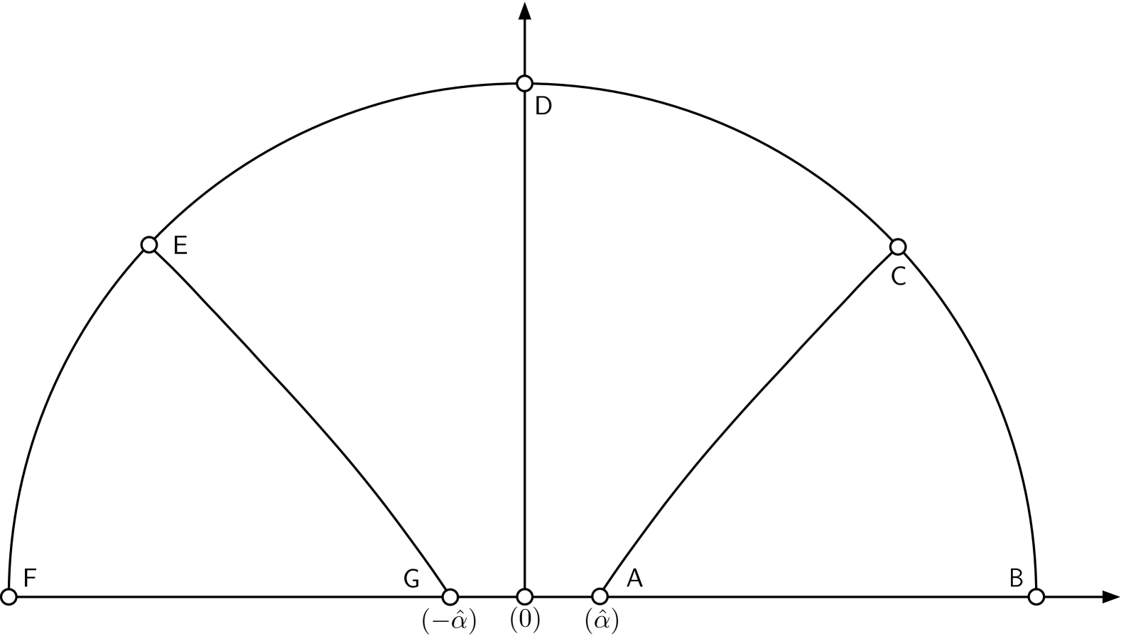
Figure 1: $\zeta$ plane.

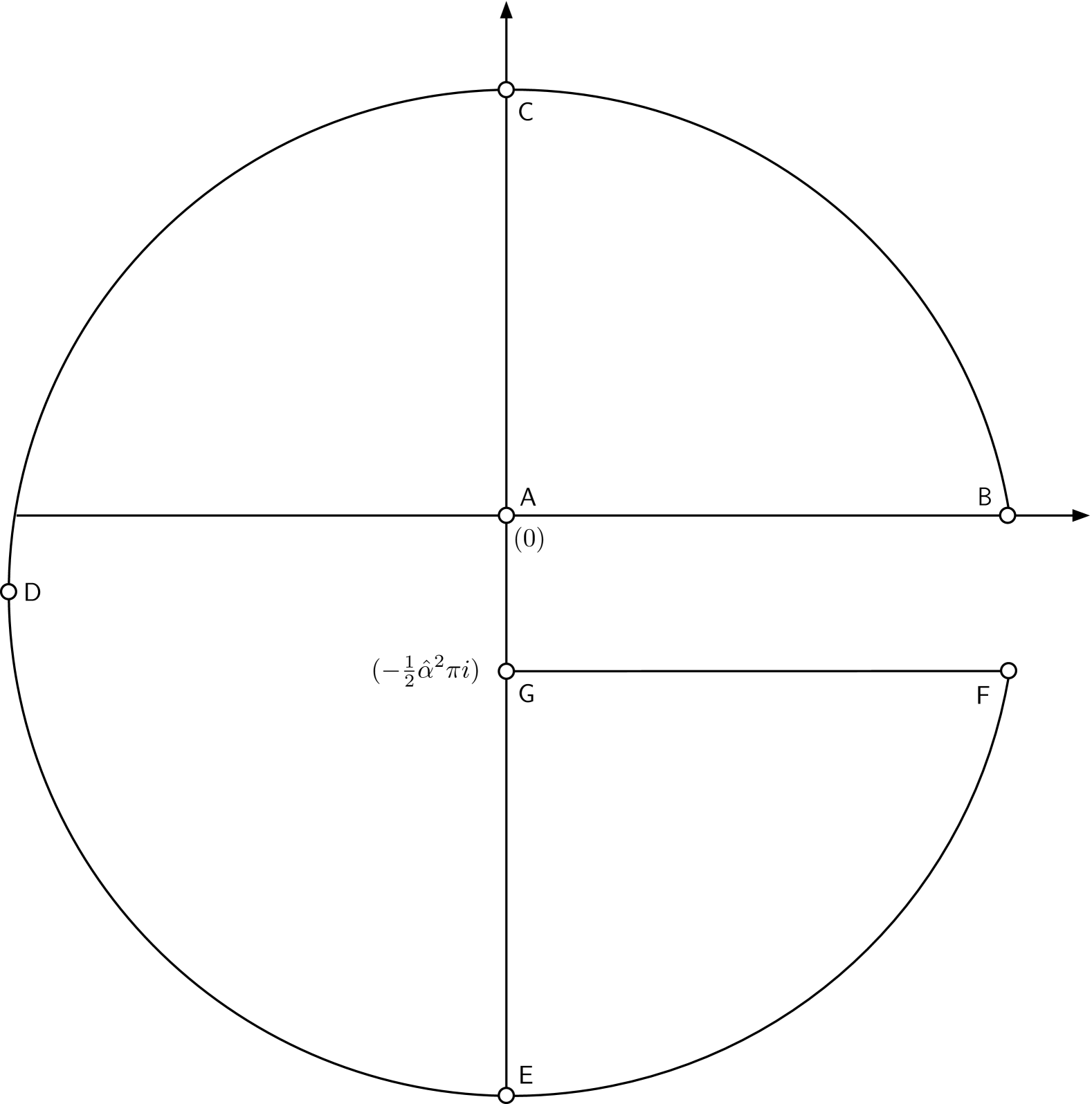
Figure 2: $\hat{\xi}$ plane.

(50) $$\hat{\xi}=\frac{1}{2}\zeta^{2}-\frac{1}{4}\hat{\alpha}^{2}\left\{2\ln\left(\frac{2\zeta}{\hat{\alpha}}\right)+1\right\}+\mathcal{O}\left(\frac{1}{\zeta^{2}}\right).$$

The map of the upper $\zeta$ half plane to the $\hat{\xi}$ plane is shown in Figs. 1 and 2 with certain corresponding points labeled. The map of the lower half-plane is the conjugate of this. Thus, for example, at the points labeled $\mathsf{F}$, we observe $\hat{\xi}\to\infty-\frac{1}{2}\hat{\alpha}^{2}\pi i$ as $\zeta\to-\infty+i0$ (see also (50)). Similarly $\hat{\xi}\to\infty+\frac{1}{2}\hat{\alpha}^{2}\pi i$ as $\zeta\to-\infty-i0$ in the conjugate regions.

In Section 4, our subsequent application to solutions of (1) at the turning points of that equation, we shall take $\zeta$ to be defined by (8), which will depend on $z$ and $\alpha$ (as given by Eq. 11). However, in what follows in this section, we consider it to be a general independent variable.

Now, let $\Theta_{1}$ be the upper half of the $\zeta$ plane ($\Im(\zeta)\geq 0$) with small neighborhoods of the turning points $\zeta=\pm\hat{\alpha}$ excluded, and $\Theta_{3}$ the conjugate region. Let $\Theta_{2}$ be the region in the $\zeta$ plane where $|\arg(\zeta)|\leq\frac{3}{4}\pi$ with a small neighborhood of the interval $[0,\hat{\alpha}]$ excluded. Let $\Theta_{4}^{+}$ be the region in the $\zeta$ plane where $\frac{1}{4}\pi\leq\arg(\zeta)\leq\pi$ with a small neighborhood of the interval $[-\hat{\alpha},0]$ excluded, and finally let $\Theta_{4}^{-}$ be the conjugate of this. These are regions in which our respective LG expansions will be valid, and they all exclude the turning points as required. They are not maximal regions of asymptotic validity, but rather ones that are sufficiently large for our purposes.

On examination of Figs. 1 and 2 we see that the $\hat{\xi}$ region corresponding to $\Theta_{1}$ consists of all points shown in the illustrated part of the $\hat{\xi}$ plane, except for points at or near $\hat{\xi}=0$ and $\hat{\xi}=-\frac{1}{2}\hat{\alpha}^{2}\pi i$ (corresponding to the turning points $\zeta=\hat{\alpha}$ and $\zeta=-\hat{\alpha}+i0$). All points in this region can be accessed by a polygonal path linking them to $\hat{\xi}=-\infty$ (corresponding to $\zeta=i\infty$) in which $\Re(u\hat{\xi})$ is monotonic. Similarly, the $\hat{\xi}$ map of $\Theta_{3}$ consists of all points that can be accessed by a polygonal path linking them to $\hat{\xi}=-\infty$ (corresponding to $\zeta=-i\infty$) in which $\Re(u\hat{\xi})$ is again monotonic.

Likewise, the $\hat{\xi}$ region corresponding to $\Theta_{2}$ consists of points that can be accessed by a polygonal path linking them to $\hat{\xi}=+\infty$ (corresponding to $\zeta=+\infty$) in which $\Re(u\hat{\xi})$ is monotonic. Finally, $\hat{\xi}$ regions corresponding to $\Theta_{4}^{\pm}$ consist of points that can be accessed by a polygonal path that links them to $\hat{\xi}=\infty\mp\frac{1}{2}\hat{\alpha}^{2}\pi i$ (corresponding to $\zeta=-\infty\pm i0$) in which $\Re(u\hat{\xi})$ is monotonic.

Now, from [4, Eq. (1.6)] with $z=\zeta$, $f=\zeta^{2}-\hat{\alpha}^{2}$ and $g=0$, one obtains

(51) $$\hat{\psi}(\hat{\alpha},\zeta)=-\frac{3\zeta^{2}+2\hat{\alpha}^{2}}{4\left(\zeta^{2}-\hat{\alpha}^{2}\right)^{3}}.$$

Next, in order to evaluate the coefficients given by [4, Eqs. (1.9) - (1.12)], we find it helpful to introduce the variable

(52) $$\hat{\beta}=\frac{\zeta}{\hat{\alpha}^{2}\left(\zeta^{2}-\hat{\alpha}^{2}\right)^{1/2}}-\frac{1}{\hat{\alpha}^{2}}\quad(\hat{\alpha}>0),$$

where the branch of the square root is positive for $\zeta>\hat{\alpha}$ and is continuous in the plane having a cut along $[-\hat{\alpha},\hat{\alpha}]$. In the limit $\hat{\alpha}\to 0$

(53) $$\hat{\beta}=\frac{1}{2\zeta^{2}}\quad(\hat{\alpha}=0).$$

We have from Eq. 52

(54) $$\zeta=\frac{\hat{\alpha}^{2}\hat{\beta}+1}{\left\{\hat{\beta}\left(\hat{\alpha}^{2}\hat{\beta}+2\right)\right\}^{1/2}}.$$

Now from (49) it follows that $d\hat{\xi}/d\zeta=(\zeta^{2}-\hat{\alpha}^{2})^{1/2}$, and hence

(55) $$\frac{d\hat{\beta}}{d\hat{\xi}}=\frac{d\hat{\beta}}{d\zeta}\left(\frac{d\hat{\xi}}{d\zeta}\right)^{-1}=-\hat{\beta}^{2}\left(\hat{\alpha}^{2}\hat{\beta}+2\right)^{2}.$$

Thus, for the coefficients [4, Eq. (1.9)], let us denote $E_{s}(\xi)=e_{s}(\hat{\alpha},\hat{\beta})$. Then we find, using Eqs. 51, 52, 54, and 55, and [4, Eqs. (1.10) - (1.12)], that

(56) $$e_{1}(\hat{\alpha},\hat{\beta})=\tfrac{1}{24}\hat{\beta}\left(5\hat{\alpha}^{4}\hat{\beta}^{2}+15\hat{\alpha}^{2}\hat{\beta}+9\right),$$

(57) $$e_{2}(\hat{\alpha},\hat{\beta})=\tfrac{1}{16}\hat{\beta}^{2}\left(\hat{\alpha}^{2}\hat{\beta}+2\right)^{2}\left(5\hat{\alpha}^{4}\hat{\beta}^{2}+10\hat{\alpha}^{2}\hat{\beta}+3\right),$$

and for $s=2,3,4\ldots$

(58) $$e_{s+1}(\hat{\alpha},\hat{\beta})=\frac{1}{2}\hat{\beta}^{2}\left(\hat{\alpha}^{2}\hat{\beta}+2\right)^{2}\frac{\partial e_{s}(\hat{\alpha},\hat{\beta})}{\partial\hat{\beta}}\\ +\frac{1}{2}\int_{0}^{\hat{\beta}}p^{2}\left(\hat{\alpha}^{2}p+2\right)^{2}\sum\limits_{j=1}^{s-1}\frac{\partial e_{j}(\hat{\alpha},p)}{\partial p}\frac{\partial e_{s-j}(\hat{\alpha},p)}{\partial p}dp.$$

Note that $e_{s}(\hat{\alpha},0)=0$ ($s=1,2,3,\ldots$). Furthermore, using a similar argument to (24), the even coefficients $e_{2s}(\hat{\alpha},\hat{\beta})$ are meromorphic at $\zeta=\pm\hat{\alpha}$ when regarded as functions of $\zeta$, and the odd ones $e_{2s+1}(\hat{\alpha},\hat{\beta})$ when regarded as functions of $\zeta$ have a branch cut along $[-\hat{\alpha},\hat{\alpha}]$, and are analytic at all points away from this interval.

We can now apply [4, Thm. 1.1] to obtain the solutions

(59) $$\hat{W}_{n,j}(u,\hat{\alpha},\zeta)=\exp\left\{u\hat{\xi}+\sum\limits_{s=1}^{n-1}{\frac{e_{s}(\hat{\alpha},\hat{\beta})}{u^{s}}}\right\}\left\{1+\hat{\eta}_{n,j}(u,\hat{\alpha},\zeta)\right\}\quad(j=1,3),$$

(60) $$\hat{W}_{n,2}(u,\hat{\alpha},\zeta)=\exp\left\{-u\hat{\xi}+\sum\limits_{s=1}^{n-1}{(-1)^{s}\frac{e_{s}(\hat{\alpha},\hat{\beta})}{u^{s}}}\right\}\left\{1+\hat{\eta}_{n,2}(u,\hat{\alpha},\zeta)\right\},$$

and

(61) $$\hat{W}_{n,4}^{\pm}(u,\hat{\alpha},\zeta)=\exp\left\{-u\hat{\xi}+\sum\limits_{s=1}^{n-1}{(-1)^{s}\frac{e_{s}(\hat{\alpha},\hat{\beta})}{u^{s}}}\right\}\left\{1+\hat{\eta}_{n,4}^{\pm}(u,\hat{\alpha},\zeta)\right\}.$$

Similarly to (28), the LG solutions $\hat{W}_{n,4}^{\pm}(u,\hat{\alpha},\zeta)$ only differ by a multiplicative constant, and their $\zeta$ regions of validity $\Theta_{4}^{\pm}$ (where $\hat{\eta}_{n,4}^{\pm}(u,\hat{\alpha},\zeta)=\mathcal{O}(u^{-n})$ as $u\to\infty$) differ.

For $\zeta\in\Theta_{j}$ ($j=1,2,3$) we again apply [4, Thm. 1.1], and consequently bounds on the error terms are given by

(62) $$\left|\hat{\eta}_{n,j}(u,\zeta)\right|\leq|u|^{-n}\omega_{n,j}(u,\hat{\beta})\exp\left\{|u|^{-1}\varpi_{n,j}(u,\hat{\beta})+|u|^{-n}\omega_{n,j}(u,\hat{\beta})\right\},$$

where

(63) $$\omega_{n,j}(u,a,\hat{\beta})=2\int_{0}^{\hat{\beta}}{\left|\frac{\partial e_{n}(\hat{\alpha},p)}{\partial p}dp\right|}\\ +\sum\limits_{s=1}^{n-1}\frac{1}{|u|^{s}}\sum\limits_{k=s}^{n-1}\int_{0}^{\hat{\beta}}{\left|p^{2}\left(\hat{\alpha}^{2}p+2\right)^{2}\frac{\partial e_{k}(\hat{\alpha},p)}{\partial p}\frac{\partial e_{s+n-k-1}(\hat{\alpha},p)}{\partial p}dp\right|},$$

and

(64) $$\varpi_{n,j}(u,\hat{\beta})=4\sum\limits_{s=0}^{n-2}\frac{1}{|u|^{s}}\int_{0}^{\hat{\beta}}\left|\frac{\partial e_{s+1}(\hat{\alpha},p)}{\partial p}dp\right|.$$

These bounds also hold for $\hat{\eta}_{n,4}^{\pm}(u,\zeta)$ for $\zeta\in\Theta_{4}^{\pm}$ .

Integration is taken along paths that correspond to paths in the $\hat{\xi}$ plane as described above in the definitions of the regions of validity. The lower integration limits $\hat{\beta}=0$ are chosen to correspond to $\zeta=\pm i\infty$ for $j=1,3$, respectively, $\zeta=+\infty$ for $j=2$, and $\zeta=-\infty\pm i0$ for the bounds for $\hat{\eta}_{n,4}^{\pm}(u,\zeta)$.

Matching solutions recessive at $\zeta=\pm\infty$ and $\zeta=\pm i\infty$, and using Eqs. 15 and 50, provides the following:

(65) $$U\left(\tfrac{1}{2}u\hat{\alpha}^{2},-i\sqrt{2u}\,\zeta\right)=\left(\frac{2e}{u\hat{\alpha}^{2}}\right)^{\frac{1}{4}u\hat{\alpha}^{2}}\frac{e^{\frac{1}{4}(u\hat{\alpha}^{2}+1)\pi i}}{\left\{2u\left(\zeta^{2}-\hat{\alpha}^{2}\right)\right\}^{1/4}}\hat{W}_{n,1}(u,\hat{\alpha},\zeta),$$

(66) $$U\left(\tfrac{1}{2}u\hat{\alpha}^{2},i\sqrt{2u}\,\zeta\right)=\left(\frac{2e}{u\hat{\alpha}^{2}}\right)^{\frac{1}{4}u\hat{\alpha}^{2}}\frac{e^{-\frac{1}{4}(u\hat{\alpha}^{2}+1)\pi i}}{\left\{2u\left(\zeta^{2}-\hat{\alpha}^{2}\right)\right\}^{1/4}}\hat{W}_{n,3}(u,\hat{\alpha},\zeta),$$

(67) $$U\left(-\tfrac{1}{2}u\hat{\alpha}^{2},\sqrt{2u}\,\zeta\right)=\left(\frac{u\hat{\alpha}^{2}}{2e}\right)^{\frac{1}{4}u\hat{\alpha}^{2}}\frac{1}{\left\{2u\left(\zeta^{2}-\hat{\alpha}^{2}\right)\right\}^{1/4}}\hat{W}_{n,2}(u,\hat{\alpha},\zeta),$$

and

(68) $$U\left(-\tfrac{1}{2}u\hat{\alpha}^{2},-\sqrt{2u}\,\zeta\right)=\pm ie^{\mp\frac{1}{2}u\hat{\alpha}^{2}\pi i}\left(\frac{u\hat{\alpha}^{2}}{2e}\right)^{\frac{1}{4}u\hat{\alpha}^{2}}\\ \times\frac{1}{\left\{2u\left(\zeta^{2}-\hat{\alpha}^{2}\right)\right\}^{1/4}}\hat{W}_{n,4}^{\pm}(u,\hat{\alpha},\zeta),$$

where we recall that the coefficients $e_{s}(\hat{\alpha},\hat{\beta})$ vanish at $|\zeta|=\infty$ ($\hat{\beta}=0$).

Next, for derivatives from (13), we arrive at

(69) $$\frac{d^{2}\tilde{w}}{d\zeta^{2}}=\left\{u^{2}\left(\zeta^{2}-\hat{\alpha}^{2}\right)+\frac{2\zeta^{2}+\hat{\alpha}^{2}}{\left(\zeta^{2}-\hat{\alpha}^{2}\right)^{2}}\right\}\tilde{w},$$

whose solutions are given by

(70) $$\tilde{w}=(\zeta^{2}-\hat{\alpha}^{2})^{-1/2}\partial w/\partial\zeta,$$

where $w=U(-\frac{1}{2}u\hat{\alpha}^{2},\sqrt{2u}\,\zeta)$ or any other solution of (13). Now, again with $f=\zeta^{2}-\hat{\alpha}^{2}$, but instead of $g=0$ now with $g=(2\zeta^{2}+\hat{\alpha}^{2})/(\zeta^{2}-\hat{\alpha}^{2})^{2}$, we have in place of (51)

(71) $$\tilde{\psi}(\hat{\alpha},\zeta)=\frac{5\zeta^{2}+2\hat{\alpha}^{2}}{4\left(\zeta^{2}-\hat{\alpha}^{2}\right)^{3}}.$$

Then, similarly to Eqs. 56, 57, and 58, we obtain

(72) $$\tilde{e}_{1}(\hat{\alpha},\hat{\beta})=-\tfrac{1}{24}\hat{\beta}\left(7\hat{\alpha}^{4}\hat{\beta}^{2}+21\hat{\alpha}^{2}\hat{\beta}+15\right),$$

and

(73) $$\tilde{e}_{2}(\hat{\alpha},\hat{\beta})=-\tfrac{1}{16}\hat{\beta}^{2}\left(\hat{\alpha}^{2}\hat{\beta}+2\right)^{2}\left(7\hat{\alpha}^{4}\hat{\beta}^{2}+14\hat{\alpha}^{2}\hat{\beta}+5\right),$$

with $\hat{\beta}$ also given by (52) and subsequent coefficients by (58). Again, $\tilde{e}_{2s}(\hat{\alpha},\hat{\beta})$ are meromorphic at $\zeta=\pm\hat{\alpha}$ when regarded as functions of $\zeta$, and $\tilde{e}_{2s+1}(\hat{\alpha},\hat{\beta})$ when regarded as functions of $\zeta$ are analytic at all points away from the interval $[-\hat{\alpha},\hat{\alpha}]$.

The LG solutions to (69) are given by $\tilde{w}_{n,j}(u,\hat{\alpha},\zeta)=(\zeta^{2}-\hat{\alpha}^{2})^{-1/4}\tilde{W}_{n,j}(u,\hat{\alpha},\zeta)$ where

(74) $$\tilde{W}_{n,j}(u,\hat{\alpha},\zeta)=\exp\left\{u\hat{\xi}+\sum\limits_{s=1}^{n-1}{\frac{\tilde{e}_{s}(\hat{\alpha},\hat{\beta})}{u^{s}}}\right\}\left\{1+\tilde{\eta}_{n,j}(u,\hat{\alpha},\zeta)\right\}\quad(j=1,3),$$

(75) $$\tilde{W}_{n,2}(u,\hat{\alpha},\zeta)=\exp\left\{-u\hat{\xi}+\sum\limits_{s=1}^{n-1}{(-1)^{s}\frac{\tilde{e}_{s}(\hat{\alpha},\hat{\beta})}{u^{s}}}\right\}\left\{1+\tilde{\eta}_{n,2}(u,\hat{\alpha},\zeta)\right\},$$

and

(76) $$\tilde{W}_{n,4}^{\pm}(u,\hat{\alpha},\zeta)=\exp\left\{-u\hat{\xi}+\sum\limits_{s=1}^{n-1}{(-1)^{s}\frac{\tilde{e}_{s}(\hat{\alpha},\hat{\beta})}{u^{s}}}\right\}\left\{1+\tilde{\eta}_{n,4}^{\pm}(u,\hat{\alpha},\zeta)\right\}.$$

Error bounds and regions of validity are the same as those for the corresponding non-derivative functions, except of course with the different coefficients.

Now, using Eqs. 16 and 50, we can match solutions recessive at $\zeta=\pm\infty$ and $\zeta=\pm i\infty$, and as a result we have

(77) $$U^{\prime}\left(\tfrac{1}{2}u\hat{\alpha}^{2},-i\sqrt{2u}\,\zeta\right)=-e^{\frac{1}{4}(u\hat{\alpha}^{2}-1)\pi i}\left(\frac{2e}{u\hat{\alpha}^{2}}\right)^{\frac{1}{4}u\hat{\alpha}^{2}}\left\{\frac{1}{8}u\left(\zeta^{2}-\hat{\alpha}^{2}\right)\right\}^{1/4}\tilde{W}_{n,1}(u,\hat{\alpha},\zeta),$$

(78) $$U^{\prime}\left(\tfrac{1}{2}u\hat{\alpha}^{2},i\sqrt{2u}\,\zeta\right)=-e^{-\frac{1}{4}(u\hat{\alpha}^{2}-1)\pi i}\left(\frac{2e}{u\hat{\alpha}^{2}}\right)^{\frac{1}{4}u\hat{\alpha}^{2}}\left\{\frac{1}{8}u\left(\zeta^{2}-\hat{\alpha}^{2}\right)\right\}^{1/4}\tilde{W}_{n,3}(u,\hat{\alpha},\zeta),$$

(79) $$U^{\prime}\left(-\tfrac{1}{2}u\hat{\alpha}^{2},\sqrt{2u}\,\zeta\right)=-\left(\frac{u\hat{\alpha}^{2}}{2e}\right)^{\frac{1}{4}u\hat{\alpha}^{2}}\left\{\frac{1}{8}u\left(\zeta^{2}-\hat{\alpha}^{2}\right)\right\}^{1/4}\tilde{W}_{n,2}(u,\hat{\alpha},\zeta),$$

and

(80) $$U^{\prime}\left(-\tfrac{1}{2}u\hat{\alpha}^{2},-\sqrt{2u}\,\zeta\right)=\pm ie^{\mp\frac{1}{2}u\hat{\alpha}^{2}\pi i}\left(\frac{u\hat{\alpha}^{2}}{2e}\right)^{\frac{1}{4}u\hat{\alpha}^{2}}\\ \times\left\{\frac{1}{8}u\left(\zeta^{2}-\hat{\alpha}^{2}\right)\right\}^{1/4}\tilde{W}_{n,4}^{\pm}(u,\hat{\alpha},\zeta).$$

4 Expansions valid at the turning points

Here we use the results of the previous two sections to construct asymptotic expansions for solutions of (1) that are valid at the two turning points. To this end, we first define two slowly varying functions, which we denote by $\mathcal{A}(u,a,z)$ and $\mathcal{B}(u,a,z)$, by the pair of equations

(81) $$w_{n,1}(u,a,z)=e^{-\frac{1}{4}(u\hat{\alpha}^{2}-1)\pi i}\Biggl{\{}U\left(\tfrac{1}{2}u\hat{\alpha}^{2},-i\sqrt{2u}\,\zeta\right)\mathcal{A}(u,a,z)\Biggr{.}\\ \left.+\frac{\partial U\left(\tfrac{1}{2}u\hat{\alpha}^{2},-i\sqrt{2u}\,\zeta\right)}{\partial\zeta}\mathcal{B}(u,a,z)\right\},$$

and

(82) $$w_{n,3}(u,a,z)=e^{\frac{1}{4}(u\hat{\alpha}^{2}-1)\pi i}\Biggl{\{}U\left(\tfrac{1}{2}u\hat{\alpha}^{2},i\sqrt{2u}\,\zeta\right)\mathcal{A}(u,a,z)\Biggr{.}\\ \left.+\frac{\partial U\left(\tfrac{1}{2}u\hat{\alpha}^{2},i\sqrt{2u}\,\zeta\right)}{\partial\zeta}\mathcal{B}(u,a,z)\right\},$$

where $w_{n,1}(u,a,z)$ and $w_{n,3}(u,a,z)$ are the solutions defined by Eqs. 18 and 19, which are recessive at the singularities $z=x_{1}$ and $z=x_{3}$, respectively. Note that $U(\tfrac{1}{2}u\hat{\alpha}^{2},-i\sqrt{2u}\,\zeta)$ is recessive at $\zeta=i\infty$, which corresponds to $z=x_{1}$, and thus the RHS of (81) matches the recessive behavior of the function on the LHS of the equation. Likewise, both sides of (82) have a matching recessive behavior at $z=x_{3}$ ($\zeta=-i\infty$).

The multiplicative constants on the RHS of Eqs. 81 and 82 were chosen to produce, on referring to Eqs. 45 and 30,

(83) $$w_{n,2}(u,a,z)=\frac{\sqrt{2\pi}}{\Gamma\left(\tfrac{1}{2}u\hat{\alpha}^{2}+\tfrac{1}{2}\right)}\Biggl{\{}U\left(-\tfrac{1}{2}u\hat{\alpha}^{2},\sqrt{2u}\,\zeta\right)\mathcal{A}(u,a,z)\Biggr{.}\\ \left.+\frac{\partial U\left(-\tfrac{1}{2}u\hat{\alpha}^{2},\sqrt{2u}\,\zeta\right)}{\partial\zeta}\mathcal{B}(u,a,z)\right\}.$$

Again we see that both sides have the same recessive behavior at a singularity, in this case at $z=x_{2}$ ($\zeta=+\infty$).

We need a similar representation for $w_{n,4}(u,a,z)$ that involves $U(-\tfrac{1}{2}u\hat{\alpha}^{2},-\sqrt{2u}\,\zeta)$ and its derivative, both of which are recessive at $z=x_{4}$ ($\zeta=-\infty$). This is achieved by defining $\hat{\alpha}$ by

(84) $$\tfrac{1}{2}u\hat{\alpha}^{2}=\lambda+\tfrac{1}{2},$$

where $\lambda$ is the connection coefficient that is defined via (31). Then from Eqs. 31, 45, 81, 82, and 84 we arrive at our desired representation

(85) $$w_{n,4}(u,a,z)=\frac{\sqrt{2\pi}}{\Gamma\left(\tfrac{1}{2}u\hat{\alpha}^{2}+\tfrac{1}{2}\right)}\Biggl{\{}U\left(-\tfrac{1}{2}u\hat{\alpha}^{2},-\sqrt{2u}\,\zeta\right)\mathcal{A}(u,a,z)\Biggr{.}\\ \left.+\frac{\partial U\left(-\tfrac{1}{2}u\hat{\alpha}^{2},-\sqrt{2u}\,\zeta\right)}{\partial\zeta}\mathcal{B}(u,a,z)\right\}.$$

Solving Eqs. 81 and 83, and using the Wronskian (43), yields the explicit formulas

(86) $$\mathcal{A}(u,a,z)=\frac{e^{-\frac{1}{4}(u\hat{\alpha}^{2}+1)\pi i}\Gamma\left(\tfrac{1}{2}u\hat{\alpha}^{2}+\tfrac{1}{2}\right)}{2\sqrt{u\pi}}\left\{w_{n,2}(u,a,z)\frac{\partial U\left(\tfrac{1}{2}u\hat{\alpha}^{2},-i\sqrt{2u}\,\zeta\right)}{\partial\zeta}\right.\\ \left.+\frac{i}{\sqrt{2u}}w_{n,1}(u,a,z)\frac{\partial U\left(-\tfrac{1}{2}u\hat{\alpha}^{2},\sqrt{2u}\,\zeta\right)}{\partial\zeta}\right\},$$

and

(87) $$\mathcal{B}(u,a,z)=-\frac{e^{-\frac{1}{4}(u\hat{\alpha}^{2}+1)\pi i}\Gamma\left(\tfrac{1}{2}u\hat{\alpha}^{2}+\tfrac{1}{2}\right)}{2\sqrt{u\pi}}\left\{w_{n,2}(u,a,z)U\left(\tfrac{1}{2}u\hat{\alpha}^{2},-i\sqrt{2u}\,\zeta\right)\right.\\ \left.-\frac{i}{\sqrt{2u}}w_{n,1}(u,a,z)U\left(-\tfrac{1}{2}u\hat{\alpha}^{2},\sqrt{2u}\,\zeta\right)\right\}.$$

Similar representations can be obtained by choosing any pair of Eqs. 81, 82, 83, and 85.

The plan is to replace the six functions $w_{n,j}(u,a,z)$ ($j=1,2$), $U(-\tfrac{1}{2}u\hat{\alpha}^{2},\sqrt{2u}\,\zeta)$, $\partial U(-\tfrac{1}{2}u\hat{\alpha}^{2},\sqrt{2u}\,\zeta)/\partial\zeta$, $U(\tfrac{1}{2}u\hat{\alpha}^{2},-i\sqrt{2u}\,\zeta)$ and $\partial U(\tfrac{1}{2}u\hat{\alpha}^{2},-i\sqrt{2u}\,\zeta)/\partial\zeta$ in Eqs. 86 and 87 by their LG expansions, and likewise in other sectors containing numerically satisfactory sets of functions. This provides a method of asymptotically evaluating the two coefficient functions in certain regions described next, since each product pair in the expression involves one recessive and one dominant solution in the region under consideration.

Let us then examine the regions of asymptotic validity in this method. To this end, define

(88) $$D=\left\{Z_{1}\cap Z_{2}\right\}\cup\left\{Z_{1}\cap Z_{4}^{+}\right\}\cup\left\{Z_{3}\cap Z_{2}\right\}\cup\left\{Z_{3}\cap Z_{4}^{-}\right\}.$$

This surrounds, but does not contain, the interval $[z_{1},z_{2}]$. The significance of $D$ is that any numerically satisfactory pair of LG expansions is asymptotically valid in this domain. We also need to utilize LG expansions for parabolic cylinder functions, and as such we also need to exclude the points where they are not all valid, namely those corresponding to the $\zeta$ interval $[-\hat{\alpha},\hat{\alpha}]$. Now, we know that $\zeta(z_{1})=-\alpha$ and $\zeta(z_{2})=\alpha$. This leads to the following.

Definition 4.1.

Let $z=\hat{z}_{1}$ and $z=\hat{z}_{2}$ correspond to $\zeta=\pm\hat{\alpha}$, so that $\zeta(\hat{z}_{1})=-\hat{\alpha}$ and $\zeta(\hat{z}_{2})=\hat{\alpha}$. Let $J$ be the curve in the $z$ plane with end points $\hat{z}_{1}$ and $\hat{z}_{2}$, corresponding to the $\zeta$ interval $[-\hat{\alpha},\hat{\alpha}]$. Then for any $\delta>0$ we define $I(\delta)=\{z:|z-v|<\delta,\forall v\in[z_{1},z_{2}]\cup J\}$; in other words, $I(\delta)$ consists of all points within a distance $\delta$ of $[z_{1},z_{2}]\cup J$.

Note that $J$ would be the interval $[\hat{z}_{1},\hat{z}_{2}]$ if $\hat{\alpha}$ were real. We also observe that, for large $u$, the point sets $[z_{1},z_{2}]$ and $J$ are close to each other, since from Eqs. 37 and 84 $\hat{\alpha}=\alpha+\mathcal{O}(u^{-2})$ as $u\to\infty$.

For $z\in D\setminus I(\delta)$ we can then use both the LG expansions of the general equation given in Section 2, as well as those for parabolic cylinder functions given in Section 3. Thus, we can use the appropriate LG expansions from Eqs. 18, 19, 20, 28, 29, 59, 60, 61, 65, 66, 67, 68, 74, 75, 76, 77, 78, 79, and 80 in Eqs. 86 and 87, and as a result we find that the same expansions are obtained regardless of which pair is chosen, namely

(89) $$\mathcal{A}(u,a,z)\sim\frac{(2u)^{1/4}}{2}\left(\frac{\zeta^{2}-\hat{\alpha}^{2}}{f(a,z)}\right)^{1/4}\left[K_{n,2}(u,a)\exp\left\{u(\hat{\xi}-\xi)+\sum_{s=1}^{\infty}(-1)^{s}\frac{\tilde{\mathcal{E}}_{s}(a,z)}{u^{s}}\right\}\right.\\ \left.-K_{n,1}(u,a)\exp\left\{-u(\hat{\xi}-\xi)+\sum_{s=1}^{\infty}\frac{\tilde{\mathcal{E}}_{s}(a,z)}{u^{s}}\right\}\right],$$

and

(90) $$\mathcal{B}(u,a,z)\sim-\frac{1}{(2u)^{3/4}}\frac{1}{\left\{f(a,z)\left(\zeta^{2}-\hat{\alpha}^{2}\right)\right\}^{1/4}}\\ \times\left[K_{n,2}(u,a)\exp\left\{u(\hat{\xi}-\xi)+\sum_{s=1}^{\infty}(-1)^{s}\frac{\mathcal{E}_{s}(a,z)}{u^{s}}\right\}\right.\\ \left.+K_{n,1}(u,a)\exp\left\{-u(\hat{\xi}-\xi)+\sum_{s=1}^{\infty}\frac{\mathcal{E}_{s}(a,z)}{u^{s}}\right\}\right],$$

as $u\to\infty$, both of which hold uniformly for $z\in D\setminus I(\delta)$. Here

(91) $$K_{n,1}(u,a)=i\left(\frac{2e}{u\hat{\alpha}^{2}}\right)^{-\frac{1}{4}u\hat{\alpha}^{2}}k_{n,1}(u,a),$$

(92) $$K_{n,2}(u,a)=\frac{1}{\sqrt{2\pi}}\left(\frac{2e}{u\hat{\alpha}^{2}}\right)^{\frac{1}{4}u\hat{\alpha}^{2}}\Gamma\left(\tfrac{1}{2}u\hat{\alpha}^{2}+\tfrac{1}{2}\right)k_{n,2}(u,a),$$

(93) $$\tilde{\mathcal{E}}_{s}(a,z)=\hat{E}_{s}(a,z)+(-1)^{s}\tilde{e}_{s}(\hat{\alpha},\hat{\beta}),$$

and

(94) $$\mathcal{E}_{s}(a,z)=\hat{E}_{s}(a,z)+(-1)^{s}e_{s}(\hat{\alpha},\hat{\beta}).$$

Now, as we observed above, $\hat{\alpha}^{2}=\alpha^{2}+\mathcal{O}(u^{-2})$ as $u\to\infty$. Thus, from Eqs. 49 and 8

(95) $$\hat{\xi}-\xi=\frac{1}{2}\zeta\left\{\left(\zeta^{2}-\hat{\alpha}^{2}\right)^{1/2}-\left(\zeta^{2}-\alpha^{2}\right)^{1/2}\right\}-\frac{1}{2}\hat{\alpha}^{2}\ln\left\{\zeta+\left(\zeta^{2}-\hat{\alpha}^{2}\right)^{1/2}\right\}\\ +\frac{1}{2}\alpha^{2}\ln\left\{\zeta+\left(\zeta^{2}-\alpha^{2}\right)^{1/2}\right\}+\frac{1}{2}\hat{\alpha}^{2}\ln(\hat{\alpha})-\frac{1}{2}\alpha^{2}\ln(\alpha)=\mathcal{O}\left(\frac{1}{u^{2}}\right),$$

for $\alpha\in[0,\alpha_{1}]$ and bounded $\zeta$. It can also be confirmed that $\hat{\xi}-\xi=u^{-2}\mathcal{O}\{\ln(\zeta)\}+\mathcal{O}(u^{-1})$ as $\zeta\to\infty$. Therefore, the terms $\pm u(\hat{\xi}-\xi)$ appearing in the exponents in Eqs. 89 and 90 are bounded for fixed $\zeta$ as $u\to\infty$, and contribute at worst (on exponentiation) to a slowly growing algebraic term as $\zeta\to\infty$ with $u$ large. This confirms that $\mathcal{A}(u,a,z)$ and $\mathcal{B}(u,a,z)$ are slowly varying as $u\to\infty$ and $z\in D\setminus I(\delta)$.

The above expansions break down near the turning points, and indeed are not valid in $I(\delta)$. Following [6] we can instead use Cauchy’s integral formula to obtain expansions that are valid at these points. Thus, because the functions are analytic at these turning points, we have

(96) $$\mathcal{A}(u,a,z)=\frac{1}{2\pi i}\oint_{\mathcal{C}}\frac{\mathcal{A}(u,a,t)}{t-z}dt,\,\mathcal{B}(u,a,z)=\frac{1}{2\pi i}\oint_{\mathcal{C}}\frac{\mathcal{B}(u,a,t)}{t-z}dt.$$

The contour $\mathcal{C}$ is a suitably chosen positively orientated simple loop lying in $D$ that encloses $z$ and the set $I(\delta)$. In the integrands we can then insert the expansions Eqs. 89 and 90, since they are valid on the contour. This enables an accurate evaluation of $\mathcal{A}(u,a,z)$ and $\mathcal{B}(u,a,z)$ for points inside the contour, particularly those in $I(\delta)$.

Note that Eqs. 81, 82, 83, and 84, being exact, can be differentiated with respect to $z$ to produce expansions for the derivatives of the solutions. In doing so, one uses the chain rule in conjunction with (5), as well as 13). For example, from (81)

(97) $$\frac{\partial w_{n,1}(u,a,z)}{\partial z}=e^{-\frac{1}{4}(u\hat{\alpha}^{2}-1)\pi i}\Biggl{\{}U\left(\tfrac{1}{2}u\hat{\alpha}^{2},-i\sqrt{2u}\,\zeta\right)\tilde{\mathcal{A}}(u,a,z)\Biggr{.}\\ \left.+\frac{\partial U\left(\tfrac{1}{2}u\hat{\alpha}^{2},-i\sqrt{2u}\,\zeta\right)}{\partial\zeta}\tilde{\mathcal{B}}(u,a,z)\right\},$$

where

(98) $$\tilde{\mathcal{A}}(u,a,z)=\frac{\partial\mathcal{A}(u,a,z)}{\partial z}+u^{2}\left\{\left(\zeta^{2}-\alpha^{2}\right)f(u,a,z)\right\}^{1/2}\mathcal{B}(u,a,z),$$

and

(99) $$\tilde{\mathcal{B}}(u,a,z)=\frac{\partial\mathcal{B}(u,a,z)}{\partial z}+\left\{\frac{f(u,a,z)}{\zeta^{2}-\alpha^{2}}\right\}^{1/2}\mathcal{A}(u,a,z).$$

Similarly for the other solutions. Then, for $z$ on or close to the set $I(\delta)$ we can use, in conjunction with (96),

(100) $$\frac{\partial\mathcal{A}(u,a,z)}{\partial z}=\frac{1}{2\pi i}\oint_{\mathcal{C}}\frac{\mathcal{A}(u,a,t)}{(t-z)^{2}}dt,\,\frac{\partial\mathcal{B}(u,a,z)}{\partial z}=\frac{1}{2\pi i}\oint_{\mathcal{C}}\frac{\mathcal{B}(u,a,t)}{(t-z)^{2}}dt.$$

We shall use the following, the proof of which is a straightforward modification of the one given for a closely related theorem [5, Thm. 3.1] that holds for isolated singularities.

Theorem 4.2.

Let $0<\rho_{0}<\rho_{1}$, $u>0$, $z_{0}\in\mathbb{C}$, $H(u,z)$ be an analytic function of $z$ in the open disk $D_{1}=\{z:\,|z-z_{0}|<\rho_{1}\}$, and $h_{s}(z)$ ($s=0,1,2,\ldots$) be a sequence of functions that are analytic in the annulus $R=\{z:\,\rho_{0}<|z-z_{0}|<\rho_{1}\}$. If $H(u,z)$ is known to possess the asymptotic expansion

(101) $$H(u,z)\sim\sum\limits_{s=0}^{\infty}\frac{h_{s}(z)}{u^{s}}\quad(u\rightarrow\infty),$$

in $R$, then each $h_{s}(z)$ is analytic in $D_{1}$ (except possibly having removable singularities there), and the expansion (101) actually holds for all $z\in D_{1}$.

The following provides traditional asymptotic expansions under certain conditions, and we shall illustrate this in the next section.

Theorem 4.3.

Suppose that the odd coefficients $\hat{E}_{2s+1}(a,z)$ are analytic in $D$, for example, being rational functions of $z$ and $\sigma(z):=\{(z-z_{1})(z-z_{2})\}^{1/2}$. Also suppose for $a_{0}\leq a\leq a_{1}$ that

(102) $$\frac{k_{n,1}(u,a)}{k_{n,2}(u,a)}\sim\sum_{s=0}^{\infty}\frac{\kappa_{s}(a)}{u^{s}}\quad(u\to\infty),$$

for certain constants $\kappa_{s}(a)$ with $\kappa_{0}(a)\neq 0$ (cf. Lemma 2.3). Next, assume for some fixed $z_{0}\in\mathbb{C}$, positive $\rho_{0}$, and sufficiently small $\delta>0$, that the disk $D_{0}=\{z:\,|z-z_{0}|<\rho_{0}\}$ contains $I(\delta)$ and lies inside $D\cup I(\delta)$. Then as $u\to\infty$, $\mathcal{A}(u,a,z)$ and $\mathcal{B}(u,a,z)$ possess the asymptotic expansions

(103) $$\mathcal{A}(u,a,z)\sim\Lambda_{1}(u,a)\left(\frac{\zeta^{2}-\hat{\alpha}^{2}}{f(a,z)}\right)^{1/4}\left\{1+\sum_{s=1}^{\infty}\frac{\mathrm{A}_{s}(a,z)}{u^{2s}}\right\},$$

and

(104) $$\mathcal{B}(u,a,z)\sim\Lambda_{2}(u,a)\left(\frac{\zeta^{2}-\hat{\alpha}^{2}}{f(a,z)}\right)^{1/4}\sum_{s=0}^{\infty}\frac{\mathrm{B}_{s}(a,z)}{u^{2s+2}},$$

for certain assignable constants $\Lambda_{j}(u,a)$ ($j=1,2$), uniformly for $a_{0}\leq a\leq a_{1}$ and $z\in D\cup I(\delta)$. The coefficients $\mathrm{A}_{s+1}(a,z)$ and $\mathrm{B}_{s}(a,z)$ ($s=0,1,2,\ldots$) can be evaluated by expanding Eqs. 89 and 90 into the forms Eqs. 103 and 104, and are analytic in $D\cup I(\delta)$.

Proof 4.4.

We know that the even coefficients $\hat{E}_{2s}(a,z)$ are always meromorphic at $z_{1}$ and $z_{2}$, and therefore are analytic in $D$. Now, by hypothesis, the odd coefficients $\hat{E}_{2s+1}(a,z)$ are also analytic in $D$. Hence from Theorems 2.1 and 84 it follows that $\alpha=\hat{\alpha}+\mathcal{O}(u^{-n})$ for any positive integer $n$, and therefore, similarly to the derivation of (95), $\xi-\hat{\xi}=\mathcal{O}(u^{-n})$ for $\zeta$ bounded, again for any positive integer $n$.

Consider now an annulus $R=\{z:\,\rho_{0}<|z-z_{0}|<\rho_{1}\}$ that lies within $D$, with $\rho_{0}$ defined by the hypothesis of the theorem. From this definition $I(\delta)$ lies inside $D_{0}$ for sufficiently small positive $\delta$, and therefore does not lie inside $R$. It follows from Eqs. 93 and 94 that $\tilde{\mathcal{E}}_{s}(a,z)$ and $\mathcal{E}_{s}(a,z)$ are analytic in $R$ (see also the comments after Eqs. 58 and 73.

Now for $z\in R$ we have by hypothesis, as noted above, $\xi-\hat{\xi}=\mathcal{O}(u^{-n})$ for any positive integer $n$, and consequently one can show, using Eqs. 40 and 102 and [3, Eq. 5.11.1], that Eqs. 89 and 90 can indeed be expanded into formal asymptotic series of the forms Eqs. 103 and 104. Furthermore, each $\mathrm{A}_{s}(a,z)$ and $\mathrm{B}_{s}(a,z)$ must be analytic in the annulus $R$, since, as we have shown, the same is true of all the coefficients appearing in Eqs. 89 and 90.

To extend this to $D_{0}$, and in particular $I(\delta)$, we appeal to Theorem 4.2. From this it follows under the above assumptions that the coefficients $\mathrm{A}_{s}(a,z)$ and $\mathrm{B}_{s}(a,z)$ are actually analytic in $D_{1}=\{z:\,|z-z_{0}|<\rho_{1}\}$, and in particular at both turning points (whether separated or not), and moreover the asymptotic expansions Eqs. 103 and 104 hold in this disk, and by extension to all points in $D\cup I(\delta)$.

Let us summarize the main results of this section. Consider the differential equation Eq. 1 with the assumptions on $f(a,z)$ and $g(z)$ stated in the paragraph following that equation, and in particular, for $a_{0}\leq a\leq a_{1}$ $f(a,z)$ has simple zeros at $z=z_{1}$ and $z=z_{2}$, which coalesce as $a\to a_{0}$. Define $\xi$, $\zeta$, and $\alpha$ by Eqs. 2, 8, and 11. Let coefficients $\hat{E}_{s}(a,z)$ be given by Eqs. 21, 22, and 23. For each positive integer $n$ let $w_{n,j}(u,a,z)$ ($j=1,2,3,4$) be solutions of Eq. 1 given by Eqs. 18, 19, 20, 28, and 29, which are recessive at the singularities $z=x_{j}$ ($j=1,2,3,4$) of Eq. 1 which correspond to $\zeta=i\infty$, $\zeta=+\infty$, $\zeta=-i\infty$, and $\zeta=-\infty$, respectively. Next $k_{n,j}(u,a)$ ($j=1,2,3$) and $k_{n,4}^{\pm}(u,a)$ are constants, continuous for $a_{0}\leq a\leq a_{1}$, chosen such that the connection formulas Eqs. 30 and 31 hold for some $\lambda$. Define $\hat{\xi}$ and $\hat{\beta}$ by Eqs. 49, 52, and 53, where $\hat{\alpha}$ is given by Eq. 84, and let coefficients $e_{s}(\hat{\alpha},\hat{\beta})$ and $\tilde{e}_{s}(\hat{\alpha},\hat{\beta})$ be given by Eqs. 56, 57, 72, and 73, with subsequent ones recursively given by Eq. 58. Let $D$ be a domain that surrounds, but does not contain, the set $I(\delta)$ that contains the turning points (defined by Definition 4.1), and is given by Eq. 88 along with certain LG regions of validity described at the beginning of Section 2.

Then $w_{n,j}(u,a,z)$ can be expressed in the forms Eqs. 81, 82, 83, and 85, where, for $a_{0}\leq a\leq a_{1}$ and $z\in D$, $\mathcal{A}(u,a,z)$ and $\mathcal{B}(u,a,z)$ possess the asymptotic expansions Eqs. 89 and 90. In these $K_{n,1}(u,a)$, $K_{n,2}(u,a)$, $\tilde{\mathcal{E}}_{s}(a,z)$ and $\mathcal{E}_{s}(a,z)$ are given by Eqs. 91, 92, 93, and 94.

For points in $I(\delta)$, which contains the two turning points, the coefficient functions $\mathcal{A}(u,a,z)$ and $\mathcal{B}(u,a,z)$ can be evaluated via the Cauchy integrals Eq. 96, with the expansions Eqs. 89 and 90 used on the contour, which is a simple positively orientated loop in $D$ which surrounds $z$ and both turning points.

The expansions Eqs. 89 and 90 can be expanded in the forms Eqs. 103 and 104, under conditions given in Theorem 4.3. If applicable, this gives an alternative way to asymptotically evaluate $\mathcal{A}(u,a,z)$ and $\mathcal{B}(u,a,z)$ in $I(\delta)$.

5 Associated Legendre functions

The associated Legendre function of the first and second kinds $P^{-\mu}_{\nu}(z)$ and $\boldsymbol{Q}^{\mu}_{\nu}(z)$ have the explicit representations given in [3, Eqs. 14.3.6, 14.3.7, 14.3.10]. These functions are solutions of the associated Legendre differential equation

(105) $$(z^{2}-1)\frac{d^{2}y}{dz^{2}}+2z\frac{dy}{dz}-\left\{\nu(\nu+1)+\frac{\mu^{2}}{z^{2}-1}\right\}y=0,$$

which has regular singularities at $z=\pm 1$ and $z=\infty$.

The behavior of these functions a the singularities is as follows, and throughout we assume $\mu,\nu\geq 0$. We have (see, for example, [3, Eqs. 14.8.7 and 14.8.15])

(106) $$P^{-\mu}_{\nu}(z)=\frac{1}{\Gamma(\mu+1)}\left(\frac{z-1}{2}\right)^{\mu/2}\left\{1+\mathcal{O}(z-1)\right\}\quad(z\rightarrow 1),$$

(107) $$P^{-\mu}_{\nu}(z)=\frac{\Gamma\left(\nu+\tfrac{1}{2}\right)(2z)^{\nu}}{\sqrt{\pi}\,\Gamma(\nu+\mu+1)}\left\{1+\mathcal{O}\left(\frac{1}{z}\right)\right\}\quad(z\rightarrow\infty),$$

and

(108) $$\boldsymbol{Q}^{\mu}_{\nu}(z)=\frac{\sqrt{\pi}}{\Gamma\left(\nu+\frac{3}{2}\right)(2z)^{\nu+1}}\left\{1+\mathcal{O}\left(\frac{1}{z}\right)\right\}\quad\left(z\rightarrow\infty\right).$$

These two functions are recessive at the respective singularities, and they form a numerically satisfactory pair of solutions of (105) in the half-plane $|\arg(z)|\leq\frac{1}{2}\pi$ (see [19, Chap. 5, Thm. 12.1]).

Connection formulas relating the functions are required and read as follows (see [3, Eq. 14.24.1]):

(109) $$P^{-\mu}_{\nu}\left(ze^{\pm\pi i}\right)=e^{\pm\nu\pi i}P^{-\mu}_{\nu}(z)+\frac{2}{\Gamma(\mu-\nu)}\boldsymbol{Q}^{\mu}_{\nu}(z),$$

from which

(110) $$2i\sin(\nu\pi)P^{-\mu}_{\nu}(z)=P^{-\mu}_{\nu}\left(ze^{\pi i}\right)-P^{-\mu}_{\nu}\left(ze^{-\pi i}\right).$$

Also,

(111) $$\boldsymbol{Q}^{\mu}_{\nu,\pm 1}(z)=e^{\mp\mu\pi i}\boldsymbol{Q}^{\mu}_{\nu}(z)\mp\frac{\pi i}{\Gamma(\nu-\mu+1)}P^{-\mu}_{\nu}(z).$$

Next, Ferrers functions are real-valued solutions of (105), and for $z=x\in(-1,1)$ which are given by (see [3, Eqs. 14.23.4 and 14.23.5])

(112) $$\mathsf{P}_{\nu}^{-\mu}(x)=e^{\mp\frac{1}{2}\mu\pi i}P_{\nu}^{-\mu}(x\pm i0),$$

and

(113) $$\mathsf{Q}_{\nu}^{-\mu}(x)=\tfrac{1}{2}\Gamma(\nu-\mu+1)\left\{e^{\frac{1}{2}\mu\pi i}\boldsymbol{Q}_{\nu}^{\mu}(x+i0)+e^{-\frac{1}{2}\mu\pi i}\boldsymbol{Q}_{\nu}^{\mu}(x-i0)\right\},$$

where $f(x\pm i0)=\lim_{\epsilon\to 0+}f(x\pm i\epsilon)$. From Eqs. 107 and 112 we have

(114) $$\mathsf{P}^{-\mu}_{\nu}(x)=\frac{1}{\Gamma(\mu+1)}\left(\frac{1-x}{2}\right)^{\mu/2}\left\{1+\mathcal{O}(x-1)\right\}\quad(x\rightarrow 1^{-}).$$

Thus, $\mathsf{P}_{\nu}^{-\mu}(\pm x)$ form a numerically satisfactory pair of solutions in $(-1,1)$ for $\mu\geq 0$ since $\mathsf{P}_{\nu}^{-\mu}(\pm x)$ is recessive at $x=\pm 1$. In addition, $\mathsf{P}_{\nu}^{-\mu}(x)$ and $\mathsf{Q}_{\nu}^{-\mu}(x)$ form a numerically satisfactory pair of solutions in $[0,1)$ for $\mu\geq 0$.

We require four solutions of Eq. 105 that are recessive at $z=\pm 1$ and $z=\pm i\infty$. In terms of the general equation of Section 2 these singularities are identified with $z=x_{2}$, $z=x_{4}$, $z=x_{1}$ and $z=x_{3}$, respectively. We also require all four to be continuous across the cut $[-1,1]$. The first of these is $\mathsf{P}^{-\mu}_{\nu}(z)$ as defined by the hypergeometric series [3, Eq. 14.3.1] for complex $x=z$ with $|z|<1$, and by analytic continuation elsewhere. This is analytic in the plane that has cuts along $(-\infty,-1]$ and $[1,\infty)$, and is, of course, equal to the real-valued Ferrers function $\mathsf{P}^{-\mu}_{\nu}(x)$ when $x\in(-1,1)$. The second fundamental solution is simply $\mathsf{P}^{-\mu}_{\nu}(-z)$, which is recessive at $z=-1$.

Next, we look for a solution that is recessive at $z=i\infty$ and continuous across the cut $[-1,1]$. The function $\boldsymbol{Q}^{\mu}_{\nu}(z)$ is indeed recessive at $z=i\infty$, but not continuous across the cut. So we define our desired function, labeled $\mathsf{Q}^{\mu}_{\nu,1}(z)$, to be equal to $\boldsymbol{Q}^{\mu}_{\nu}(z)$ in the upper half-plane and equal to the analytic continuation of that function across the cut $[-1,1]$. Consequently,

(115) $$\mathsf{Q}^{\mu}_{\nu,1}(z)=\begin{cases}\boldsymbol{Q}^{\mu}_{\nu}(z)&\Im(z)\geq 0\\ \boldsymbol{Q}^{\mu}_{\nu,1}(z)&\Im(z)<0\end{cases}\,.$$

This fulfills the requirement of being continuous, in fact analytic, in the $z$ plane having cuts along $(-\infty,-1]$ and $[1,\infty)$, and is recessive at $z=i\infty$ (or more precisely as $z\to\infty$ for $0\leq\arg(z)\leq\pi$).

Finally, for the fourth fundamental solution, define $\mathsf{Q}^{\mu}_{\nu,-1}(z)$ as the conjugate of $\mathsf{Q}^{\mu}_{\nu,1}(z)$, namely,

(116) $$\mathsf{Q}^{\mu}_{\nu,-1}(z)=\begin{cases}\boldsymbol{Q}^{\mu}_{\nu,-1}(z)&\Im(z)>0\\ \boldsymbol{Q}^{\mu}_{\nu}(z)&\Im(z)\leq 0\end{cases}\,,$$

this being recessive as $z\to\infty$ for $-\pi\leq\arg(z)\leq 0$. Note that $\mathsf{Q}^{\mu}_{\nu,\pm 1}(z)$ are generally not real for $z\in(-1,1)$.

Now, from [3, Eq. 14.23.2] one can show that

(117) $$\mathsf{P}^{-\mu}_{\nu}(z)=\frac{i\Gamma(\nu-\mu+1)}{\pi}\left\{e^{\frac{1}{2}\mu\pi i}\mathsf{Q}^{\mu}_{\nu,1}(z)-e^{-\frac{1}{2}\mu\pi i}\mathsf{Q}^{\mu}_{\nu,-1}(z)\right\}.$$

Similarly, from Eqs. 113, 115, and 116, we have

(118) $$\mathsf{Q}_{\nu}^{-\mu}(z)=\tfrac{1}{2}\Gamma(\nu-\mu+1)\left\{e^{\frac{1}{2}\mu\pi i}\mathsf{Q}^{\mu}_{\nu,1}(z)+e^{-\frac{1}{2}\mu\pi i}\mathsf{Q}^{\mu}_{\nu,-1}(z)\right\}.$$

Thus from Eqs. 117 and 118, and [3, Eq. 14.9.10]

(119) $$\mathsf{P}^{-\mu}_{\nu}(-z)=\frac{i\Gamma(\nu-\mu+1)}{\pi}\left\{e^{\frac{1}{2}(2\nu-\mu)\pi i}\mathsf{Q}^{\mu}_{\nu,1}(z)-e^{-\frac{1}{2}(2\nu-\mu)\pi i}\mathsf{Q}^{\mu}_{\nu,-1}(z)\right\}.$$

From Eqs. 119, 107, 111, 115, 116, and 117 we then find that

(120) $$\mathsf{P}^{-\mu}_{\nu}(z)=\frac{e^{\mp\mu\pi i/2}\Gamma\left(\nu+\tfrac{1}{2}\right)(2z)^{\nu}}{\sqrt{\pi}\,\Gamma(\nu+\mu+1)}\left\{1+\mathcal{O}\left(\frac{1}{z}\right)\right\}\quad(z\rightarrow\pm i\infty),$$

and

(121) $$\mathsf{P}^{-\mu}_{\nu}(-z)=\frac{e^{\mp(2\nu-\mu)\pi i/2}\Gamma\left(\nu+\tfrac{1}{2}\right)(2z)^{\nu}}{\sqrt{\pi}\,\Gamma(\nu+\mu+1)}\left\{1+\mathcal{O}\left(\frac{1}{z}\right)\right\}\quad(z\rightarrow\pm i\infty).$$

Next, let

(122) $$u=\nu+\frac{1}{2},\;1-a^{2}=\frac{\mu^{2}}{u^{2}}.$$

Then from Eq. 105 we have $(1-z^{2})^{1/2}\mathsf{P}^{-\mu}_{\nu}(\pm z)$ and $(1-z^{2})^{1/2}\mathsf{Q}^{\mu}_{\nu,\pm 1}(z)$ as solutions of Eq. 1, where

(123) $$f(a,z)=\frac{z^{2}-a^{2}}{\left(1-z^{2}\right)^{2}},\;g(z)=-\frac{3+z^{2}}{4\left(1-z^{2}\right)^{2}}.$$

We assume for arbitrary fixed $\delta>0$ that

(124) $$0\leq a\leq 1-\delta<1,$$

which is equivalent to $\delta^{\prime}u\leq\mu\leq u$ for arbitrary fixed $\delta^{\prime}>0$. Thus, we can identify the turning points $z=z_{j}$ ($j=1,2$) of Section 1 with $z=\pm a$, and from Eq. 124 $a_{0}=0$ and $a_{1}=1-\delta<1$. Note that the turning points coalesce as $a\to 0$, which from Eq. 122 is equivalent to $\mu=u=\nu+\frac{1}{2}$. Also, the upper bound in Eq. 124 ensures that the turning points are bounded away from the singularities $z=\pm 1$. This situation was studied in [2].

Now, from Eqs. 2 and 123

(125) $$\xi=\int_{a}^{z}f^{1/2}(a,t)dt=\int_{a}^{z}\frac{\left(t^{2}-a^{2}\right)^{1/2}}{1-t^{2}}dt\\ =\frac{\mu}{2u}\ln\left\{\frac{\left(uz+\mu X+ua^{2}\right)\left(uz+\mu X-ua^{2}\right)}{\left(1-z^{2}\right)}\right\}-\ln\left\{u(z+X)\right\}-\frac{(u-\mu)\ln(ua)}{u},$$

where

(126) $$X=\left(z^{2}-a^{2}\right)^{1/2}.$$

The branch is such that $\xi$ is positive for $a<z<1$ and continuous in the $z$ plane having cuts along $(-\infty,a]$ and $[1,\infty)$. An equivalent representation, which is useful for $a\leq z<1$, is given by

(127) $$\xi=\left(1-a^{2}\right)^{1/2}\mathrm{arctanh}\left\{\frac{1}{z}\left(\frac{z^{2}-a^{2}}{1-a^{2}}\right)^{1/2}\right\}-\mathrm{arccosh}\left(\frac{z}{a}\right).$$

Note in the limit $a\to 0$

(128) $$\xi=-\tfrac{1}{2}\ln\left(1-z^{2}\right).$$

We next record the following limiting forms:

(129) $$\xi=\frac{2\sqrt{2a}}{3\left(1-a^{2}\right)}(z-a)^{3/2}+\mathcal{O}\left\{(z-a)^{2}\right\}\quad(z\to a),$$

and

(130) $$\xi=-\frac{1}{2}\left(1-a^{2}\right)^{1/2}\ln\left\{\frac{1-z}{2\left(1-a^{2}\right)}\right\}-\ln\left\{1+\left(1-a^{2}\right)^{1/2}\right\}\\ +\left\{1-\left(1-a^{2}\right)^{1/2}\right\}\ln(a)+\mathcal{O}(z-1)\quad(z\to 1),$$

which has the following limit when $a=0$

(131) $$\xi=-\tfrac{1}{2}\ln\left\{2(1-z)\right\}+\mathcal{O}(1-z)\quad(z\to 1,\,a=0).$$

In addition,

(132) $$\xi=-\ln(2z)+\left\{1-\left(1-a^{2}\right)^{1/2}\right\}\ln(a)+\left(1-a^{2}\right)^{1/2}\ln\left\{1+\left(1-a^{2}\right)^{1/2}\right\}\\ \pm\frac{1}{2}\left(1-a^{2}\right)^{1/2}\pi i+\mathcal{O}\left(\frac{1}{z}\right)\quad\left(z\to\infty,\,\Im(z)\gtrless 0\right),$$

again with the limit applying when $a=0$, that is, $\xi=-\ln(z)\pm\frac{1}{2}\pi i+\mathcal{O}(z^{-1})$.

Consider now the LG expansions Eqs. 18, 29, 19, 20, and 28. We do not require to determine the full regions of validity $Z_{j}$ of the error term bounds Eqs. 25, 26, and 27. All we need are the following, which are straightforward to verify from the integral representation Eq. 125 of $\xi$. Firstly, $Z_{1}\cap Z_{2}$ contains all points in the first quadrant $0\leq\arg(z)\leq\frac{1}{2}\pi$, except for a small neighborhood of the interval $[0,a]$. Next, $Z_{1}\cap Z_{4}^{+}$ contains all points in the second quadrant $\frac{1}{2}\pi\leq\arg(z)\leq\pi$, except for a small neighborhood of the interval $[-a,0]$. Finally, $Z_{3}\cap Z_{2}$ and $Z_{3}\cap Z_{4}^{-}$ are conjugates of $Z_{1}\cap Z_{2}$ and $Z_{1}\cap Z_{4}^{+}$, respectively. Thus, from Eq. 88 we see that the region $D$, which we shall use for our parabolic cylinder function approximations, consists of all points in the $z$ plane having cuts along $(-\infty,-1]$ and $[1,\infty)$ and with a small neighborhood of the interval $[-a,a]$ removed.

Next, to evaluate the coefficients in the LG expansions, we first find from Eqs. 4 and 123 that

(133) $$\psi(a,z)=\frac{\left(1-z^{2}\right)\left\{(4a^{2}-3)z^{2}-a^{2}(2-a^{2})\right\}}{4\left(z^{2}-a^{2}\right)^{3}}.$$

Note that $\psi(a,z)=\mathcal{O}(1-z)$ as $z\to 1$, and also

(134) $$\psi(a,z)=\frac{3-4a^{2}}{4z^{2}}+\mathcal{O}\left(\frac{1}{z^{4}}\right)\quad(z\to\infty),$$

both of which are consequences of $f(a,z)$ and $g(z)$ defined by Eq. 123 satisfying the conditions at the beginning of Section 2 at the singularities $z=\pm 1$ and $z=\infty$.

Now let us evaluate the coefficients given by Eqs. 21, 22, and 23. In order to do so, similarly to (52), let

(135) $$\beta=\frac{z}{a^{2}\left(z^{2}-a^{2}\right)^{1/2}}-\frac{1}{a^{2}}\quad(a>0),$$

and

(136) $$\beta=\frac{1}{2z^{2}}\quad(a=0).$$

Then we denote $\hat{E}_{s}(a,z)=E_{s}(a,\beta)$ ($s=1,2,3,\ldots$), and so from Eqs. 21, 22, 23, 133, and 135, after some calculation, we obtain

(137) $$E_{1}(a,\beta)=\tfrac{1}{24}\beta\left\{5a^{4}\left(1-a^{2}\right)\beta^{2}+15a^{2}\left(1-a^{2}\right)\beta-12a^{2}+9\right\},$$

(138) $$E_{2}(a,\beta)=\tfrac{1}{16}\beta\left(a^{2}\beta+2\right)\left\{a^{2}\left(1-a^{2}\right)\beta^{2}+2\left(1-a^{2}\right)\beta-1\right\}\\ \times\left\{5a^{2}\left(1-a^{2}\right)\beta^{2}+10a^{2}\left(1-a^{2}\right)\beta-4a^{2}+3\right\},$$

and for $s=2,3,4\ldots$

(139) $$E_{s+1}(a,\beta)=\frac{1}{2}G(a,\beta)\frac{\partial E_{s}(a,\beta)}{\partial\beta}+\frac{1}{2}\int_{0}^{\beta}G(a,p)\sum\limits_{j=1}^{s-1}\frac{\partial E_{j}(a,p)}{\partial p}\frac{\partial E_{s-j}(a,p)}{\partial p}dp,$$

where

(140) $$G(a,\beta)=-d\beta/d\xi=\beta\left(a^{2}\beta+2\right)\left\{a^{2}\left(1-a^{2}\right)\beta^{2}+2\left(1-a^{2}\right)\beta-1\right\}.$$

Note that our choice of integration constants imply that $E_{s}(a,0)=0$ ($s=1,2,3,\ldots$). In addition, the odd coefficients $E_{2s+1}(a,\beta)$ ($s=0,1,2,\ldots$), considered as functions of $z$, are analytic for all points bounded away from the interval $[-a,a]$, since $\beta=\beta(z)$ is analytic in this region and each $E_{s}(a,\beta)$ is a polynomial in $\beta$. Thus $\hat{\alpha}=\alpha+\mathcal{O}(u^{-n})$ as $u\to\infty$ for any positive integer $n$. In fact, we shall show that $\hat{\alpha}=\alpha$ exactly.

Next, we identify solutions of (105) recessive at $z=\pm i\infty$ and $z=1$, with the corresponding LG expansions Eqs. 18, 29, 19, 20, and 28, which yields

(141) $$\mathsf{Q}^{\mu}_{\nu,1}(z)=\sqrt{\frac{\pi}{2}}\frac{e^{-\frac{1}{2}\mu\pi i}u^{u}}{\left(u^{2}-\mu^{2}\right)^{\frac{1}{2}u}\Gamma(u+1)}\left(\frac{u-\mu}{u+\mu}\right)^{\frac{1}{2}\mu}\frac{W_{n,1}(u,a,z)}{\left(z^{2}-a^{2}\right)^{1/4}},$$

(142) $$\mathsf{Q}^{\mu}_{\nu,-1}(z)=\sqrt{\frac{\pi}{2}}\frac{e^{\frac{1}{2}\mu\pi i}u^{u}}{\left(u^{2}-\mu^{2}\right)^{\frac{1}{2}u}\Gamma(u+1)}\left(\frac{u-\mu}{u+\mu}\right)^{\frac{1}{2}\mu}\frac{W_{n,3}(u,a,z)}{\left(z^{2}-a^{2}\right)^{1/4}},$$

and

(143) $$\mathsf{P}^{-\mu}_{\nu}(z)=\frac{\left(u^{2}-\mu^{2}\right)^{\frac{1}{2}u}\,\Gamma(u)}{\sqrt{2\pi}\,u^{u}\Gamma\left(u+\mu+\tfrac{1}{2}\right)}\left(\frac{u+\mu}{u-\mu}\right)^{\frac{1}{2}\mu}\frac{W_{n,2}(u,a,z)}{\left(z^{2}-a^{2}\right)^{1/4}}\\ \times\left\{1+\eta_{n,2}(u,a,\infty)\right\}.$$

In these, we determined the proportionality constants from Eqs. 108, 115, 116, 120, 122, and 132.

Alternatively, for (143) we can find the constant as $z\to 1$ using Eqs. 114 and 130 in place of Eqs. 120 and 132 to get

(144) $$\mathsf{P}^{-\mu}_{\nu}(z)=\left(\frac{\mu}{u}\right)^{1/4}\frac{\mu^{\mu}}{\left(u^{2}-\mu^{2}\right)^{\frac{1}{2}\mu}\Gamma(\mu+1)}\left(\frac{u-\mu}{u+\mu}\right)^{\frac{1}{2}u}\frac{W_{n,2}(u,a,z)}{\left(z^{2}-a^{2}\right)^{1/4}}\\ \times\exp\left\{\sum\limits_{s=1}^{n-1}{(-1)^{s-1}\frac{E_{s}(a,\beta_{1})}{u^{s}}}\right\},$$

where from Eqs. 122 and 135

(145) $$\beta_{1}=\beta(\pm 1)=\frac{u^{2}}{\mu(u+\mu)}.$$

Similarly,

(146) $$\mathsf{P}^{-\mu}_{\nu}(-z)=\frac{e^{\mp(\nu-\mu)\pi i}\left(u^{2}-\mu^{2}\right)^{\frac{1}{2}u}\,\Gamma(u)}{\sqrt{2\pi}\,u^{u}\Gamma\left(u+\mu+\tfrac{1}{2}\right)}\left(\frac{u+\mu}{u-\mu}\right)^{\frac{1}{2}\mu}\frac{W_{n,4}^{\pm}(u,a,z)}{\left(z^{2}-a^{2}\right)^{1/4}}\\ \times\left\{1+\eta_{n,4}^{\pm}(u,a,\pm i\infty)\right\},$$

or, alternatively,

(147) $$\mathsf{P}^{-\mu}_{\nu}(-z)=e^{\mp\frac{1}{2}(u\alpha^{2}-1)\pi i}\left(\frac{\mu}{u}\right)^{1/4}\frac{\mu^{\mu}}{\left(u^{2}-\mu^{2}\right)^{\frac{1}{2}\mu}\Gamma(\mu+1)}\left(\frac{u-\mu}{u+\mu}\right)^{\frac{1}{2}u}\\ \times\frac{W_{n,4}^{\pm}(u,a,z)}{\left(z^{2}-a^{2}\right)^{1/4}}\exp\left\{\sum\limits_{s=1}^{n-1}{(-1)^{s}\frac{E_{s}(a,\beta_{1})}{u^{s}}}\right\},$$

noting that $(z^{2}-a^{2})^{1/4}\to e^{\pm\pi i/2}(1-a^{2})^{1/4}$ as $z\to-1\pm i0$ with our choice of branches.

By comparing Eqs. 18, 29, 19, 20, and 28 with Eqs. 141, 142, 143, and 146 we can then identify

(148) $$w_{n,j}(u,a,z)=\left(1-z^{2}\right)^{1/2}e^{\pm\frac{1}{2}(\mu+1)\pi i}\mathsf{Q}^{\mu}_{\nu,\pm 1}(z),$$

for $j=1,3$, respectively, and

(149) $$w_{n,j}(u,a,z)=\frac{\pi}{\Gamma(\nu-\mu+1)}\left(1-z^{2}\right)^{1/2}\mathsf{P}^{-\mu}_{\nu}(\pm z),$$

for $j=2,4$, respectively. Furthermore, from Eqs. 141, 142, 148, and 149

(150) $$k_{n,j}(u,a)=\pm i\sqrt{\frac{\pi}{2}}\frac{u^{u}}{\left(u^{2}-\mu^{2}\right)^{\frac{1}{2}u}\Gamma(u+1)}\left(\frac{u-\mu}{u+\mu}\right)^{\frac{1}{2}\mu},$$

for $j=1,3$, respectively, and from Eqs. 143, 146, 148, and 149

(151) $$k_{n,2}(u,a)=\sqrt{\frac{\pi}{2}}\frac{\left(u^{2}-\mu^{2}\right)^{\frac{1}{2}u}\,\Gamma(u)}{u^{u}\Gamma\left(u+\mu+\tfrac{1}{2}\right)\Gamma\left(u-\mu+\tfrac{1}{2}\right)}\left(\frac{u+\mu}{u-\mu}\right)^{\frac{1}{2}\mu}\\ \times\left\{1+\eta_{n,2}(u,a,\infty)\right\},$$

and

(152) $$k_{n,4}^{\pm}(u,a)=e^{\mp(u-\mu-\frac{1}{2})\pi i}k_{n,2}(u,a)\left\{\frac{1+\eta_{n,4}^{\pm}(u,a,\pm i\infty)}{1+\eta_{n,2}(u,a,\infty)}\right\}.$$

Now let us construct our main results, namely asymptotic expansions for the Legendre functions which are valid in a domain containing the turning points. Firstly, from (11), we have

(153) $$\alpha=\left\{\frac{2}{\pi}\int_{-a}^{a}\frac{\left(a^{2}-t^{2}\right)^{1/2}}{1-t^{2}}dt\right\}^{1/2}=\left[2\left\{1-\left(1-a^{2}\right)^{1/2}\right\}\right]^{1/2},$$

i.e.

(154) $$\tfrac{1}{2}\alpha^{2}=1-\left(1-a^{2}\right)^{1/2},$$

which from (122) yields

(155) $$\tfrac{1}{2}u\alpha^{2}=\nu-\mu+\tfrac{1}{2}.$$

With this value, $\zeta=\zeta(z)$ is defined by (8), where $\xi=\xi(z)$ is given by (125) and $\alpha$ by Eq. 155. Note that when $z=x\in(-a,a)$ we have $\zeta\in(-\alpha,\alpha)$ such that

(156) $$\arcsin\left(\frac{x}{a}\right)-\left(1-a^{2}\right)^{1/2}\arctan\left\{x\left(\frac{1-a^{2}}{a^{2}-x^{2}}\right)^{1/2}\right\}\\ =\frac{1}{2}\zeta\left(\alpha^{2}-\zeta^{2}\right)^{1/2}+\frac{1}{2}\alpha^{2}\arcsin\left(\frac{\zeta}{\alpha}\right),$$

on using (154).

For $z=x\in[a,1)$ we have $\zeta\in[\alpha,\infty)$, such that

(157) $$\left(1-a^{2}\right)^{1/2}\mathrm{arctanh}\left\{\frac{1}{x}\left(\frac{x^{2}-a^{2}}{1-a^{2}}\right)^{1/2}\right\}-\mathrm{arccosh}\left(\frac{x}{a}\right)\\ =\frac{1}{2}\zeta\left(\zeta^{2}-\alpha^{2}\right)^{1/2}-\frac{1}{2}\alpha^{2}\mathrm{arccosh}\left(\frac{\zeta}{\alpha}\right).$$

If we compare Eq. 152 to Eqs. 34 and 35 we infer that $\lambda\approx u-\mu-\frac{1}{2}=\nu-\mu$ as $u\to\infty$. In fact, from Eqs. 31, 119, 148, and 149 we see that $\lambda=\nu-\mu$ exactly, and hence from Eqs. 84 and 155

(158) $$\tfrac{1}{2}u\hat{\alpha}^{2}=\nu-\mu+\tfrac{1}{2}=\tfrac{1}{2}u\alpha^{2}\implies\hat{\alpha}=\alpha.$$

Next, following Eqs. 81, 82, 155, and 148, define $\mathcal{A}(u,a,z)$ and $\mathcal{B}(u,a,z)$ by the pair of equations

(159) $$\mathsf{Q}^{\mu}_{\nu,\pm 1}(z)=e^{\mp\frac{1}{2}(\nu+1)\pi i}\Biggl{\{}U\left(\nu-\mu+\tfrac{1}{2},\mp i\sqrt{2u}\,\zeta\right)\mathcal{A}(u,a,z)\Biggr{.}\\ \left.+\frac{\partial U\left(\nu-\mu+\tfrac{1}{2},\mp i\sqrt{2u}\,\zeta\right)}{\partial\zeta}\mathcal{B}(u,a,z)\right\}.$$

Then from Eqs. 45, 117, 119, and 158

(160) $$\mathsf{P}^{-\mu}_{\nu}(\pm z)=\sqrt{\frac{2}{\pi}}\Biggl{\{}U\left(\mu-\nu-\tfrac{1}{2},\pm\sqrt{2u}\,\zeta\right)\mathcal{A}(u,a,z)\Biggr{.}\\ \left.+\frac{\partial U\left(\mu-\nu-\tfrac{1}{2},\pm\sqrt{2u}\,\zeta\right)}{\partial\zeta}\mathcal{B}(u,a,z)\right\}.$$

Also from Eqs. 48, 118, and 159

(161) $$\mathsf{Q}^{-\mu}_{\nu}(z)=\sqrt{\frac{\pi}{2}}\,\Gamma(\nu-\mu+1)\Biggl{\{}V\left(\mu-\nu-\tfrac{1}{2},\sqrt{2u}\,\zeta\right)\mathcal{A}(u,a,z)\Biggr{.}\\ \left.+\frac{\partial V\left(\mu-\nu-\tfrac{1}{2},\sqrt{2u}\,\zeta\right)}{\partial\zeta}\mathcal{B}(u,a,z)\right\}.$$

On employing the parabolic cylinder function Wronskian relations (43) we obtain, from solving the pair of equations Eqs. 159 and 160, our desired explicit formulas

(162) $$\mathcal{A}(u,a,z)=-\frac{e^{\frac{1}{2}\mu\pi i}}{2\sqrt{u}}\left\{e^{-\frac{1}{2}(\nu-1)\pi i}\sqrt{\pi}\,\mathsf{P}^{-\mu}_{\nu}(\pm z)\frac{\partial U\left(\nu-\mu+\tfrac{1}{2},-i\sqrt{2u}\,\zeta\right)}{\partial\zeta}\right.\\ \left.+\sqrt{2}\,\mathsf{Q}^{\mu}_{\nu,1}(z)\frac{\partial U\left(\mu-\nu-\tfrac{1}{2},\pm\sqrt{2u}\,\zeta\right)}{\partial\zeta}\right\},$$

and

(163) $$\mathcal{B}(u,a,z)=\frac{e^{\frac{1}{2}\mu\pi i}}{2\sqrt{u}}\left\{e^{-\frac{1}{2}(\nu-1)\pi i}\sqrt{\pi}\,\mathsf{P}^{-\mu}_{\nu}(\pm z)U\left(\nu-\mu+\tfrac{1}{2},-i\sqrt{2u}\,\zeta\right)\right.\\ \left.+\sqrt{2}\,\mathsf{Q}^{\mu}_{\nu,1}(z)U\left(\mu-\nu-\tfrac{1}{2},\pm\sqrt{2u}\,\zeta\right)\right\}.$$

Alternatively, on solving both of (160),

(164) $$\mathcal{A}(u,a,z)=\frac{\sqrt{2}\,\Gamma(\mu-\nu)}{4\sqrt{u}}\left\{\mathsf{P}^{-\mu}_{\nu}(z)\frac{\partial U\left(\mu-\nu-\tfrac{1}{2},-\sqrt{2u}\,\zeta\right)}{\partial\zeta}\right.\\ \left.-\mathsf{P}^{-\mu}_{\nu}(-z)\frac{\partial U\left(\mu-\nu-\tfrac{1}{2},\sqrt{2u}\,\zeta\right)}{\partial\zeta}\right\},$$

and

(165) $$\mathcal{B}(u,a,z)=-\frac{\sqrt{2}\,\Gamma(\mu-\nu)}{4\sqrt{u}}\left\{\mathsf{P}^{-\mu}_{\nu}(z)U\left(\mu-\nu-\tfrac{1}{2},-\sqrt{2u}\,\zeta\right)\right.\\ \left.-\mathsf{P}^{-\mu}_{\nu}(-z)U\left(\mu-\nu-\tfrac{1}{2},\sqrt{2u}\,\zeta\right)\right\},$$

which demonstrates that $\mathcal{A}(u,a,z)$ and $\mathcal{B}(u,a,z)$ are real for $z=x\in(-1,1)$, and analytic in the principal $z$ plane having cuts along $(-\infty,-1]$ and $[1,\infty)$.

Next, in a general setting, the asymptotic expansions for $\mathcal{A}(u,a,z)$ and $\mathcal{B}(u,a,z)$ come from Eqs. 89 and 90. In this specific case, we can insert Eqs. 59, 60, 65, 67, 77, 79, 74, 75, 141, and 143 into Eqs. 162 and 163 (with upper signs taken), to arrive at

(166) $$\mathcal{A}(u,a,z)=\left(\frac{\zeta^{2}-\alpha^{2}}{z^{2}-a^{2}}\right)^{1/4}\left[C_{1}(u,\alpha)\exp\left\{\sum\limits_{s=1}^{n-1}\frac{\tilde{\mathcal{E}}_{s}(a,z)}{u^{s}}\right\}\left\{1+\tilde{\delta}_{n,1}(u,a,z)\right\}\right.\\ \left.+C_{2}(u,\alpha)\exp\left\{\sum\limits_{s=1}^{n-1}(-1)^{s}\frac{\tilde{\mathcal{E}}_{s}(a,z)}{u^{s}}\right\}\left\{1+\tilde{\delta}_{n,2}(u,a,z)\right\}\right],$$

and

(167) $$\mathcal{B}(u,a,z)=\frac{1}{u\left\{\left(z^{2}-a^{2}\right)\left(\zeta^{2}-\alpha^{2}\right)\right\}^{1/4}}\left[C_{1}(u,\alpha)\exp\left\{\sum\limits_{s=1}^{n-1}\frac{\mathcal{E}_{s}(a,z)}{u^{s}}\right\}\right.\\ \left.\times\left\{1+\delta_{n,1}(u,a,z)\right\}-C_{2}(u,\alpha)\exp\left\{\sum\limits_{s=1}^{n-1}(-1)^{s}\frac{\mathcal{E}_{s}(a,z)}{u^{s}}\right\}\left\{1+\delta_{n,2}(u,a,z)\right\}\right],$$

where

(168) $$C_{1}(u,\alpha)=\frac{2^{\frac{3}{4}}\sqrt{\pi}\,e^{\frac{1}{2}(\mu-u)}u^{u-\frac{3}{4}}(u+\mu)^{-\frac{1}{2}(u+\mu)}}{4\,\Gamma(u)},$$

(169) $$C_{2}(u,\alpha)=\frac{2^{\frac{1}{4}}e^{\frac{1}{2}(u-\mu)}u^{\frac{1}{4}-u}(u+\mu)^{\frac{1}{2}(u+\mu)}\Gamma(u)}{4\,\Gamma\left(u+\mu+\tfrac{1}{2}\right)},$$

(170) $$\tilde{\mathcal{E}}_{s}(a,z)=E_{s}(a,\beta)+(-1)^{s}\tilde{e}_{s}(\alpha,\hat{\beta}),$$

(171) $$\mathcal{E}_{s}(a,z)=E_{s}(a,\beta)+(-1)^{s}e_{s}(\alpha,\hat{\beta}),$$

(172) $$\tilde{\delta}_{n,1}(u,a,z)=\left\{1+\eta_{n,1}(u,a,z)\right\}\left\{1+\tilde{\eta}_{n,2}(u,\alpha,\zeta)\right\}-1,$$

(173) $$\tilde{\delta}_{n,2}(u,a,z)=\left\{1+\tilde{\eta}_{n,1}(u,\alpha,\zeta)\right\}\left\{1+\eta_{n,2}(u,a,z)\right\}\left\{1+\eta_{n,2}(u,a,\infty)\right\}-1,$$

(174) $$\delta_{n,1}(u,a,z)=\left\{1+\eta_{n,1}(u,a,z)\right\}\left\{1+\hat{\eta}_{n,2}(u,\alpha,\zeta)\right\}-1,$$

and

(175) $$\delta_{n,2}(u,a,z)=\left\{1+\hat{\eta}_{n,1}(u,\alpha,\zeta)\right\}\left\{1+\eta_{n,2}(u,a,z)\right\}\left\{1+\eta_{n,2}(u,a,\infty)\right\}-1,$$

on recalling that $\hat{\alpha}=\alpha$ (see Eq. 158), and $\mu=(1-a^{2})^{1/2}u=(1-\frac{1}{2}\alpha^{2})u$ (see Eqs. 122 and 154).

As we showed in the more general setting, by using other pairs of Eqs. 162, 163, 164, and 165, these expansions remain valid in the full domain $D$ which includes the singularities $z=\pm 1$ and $z=\pm i\infty$, and surrounds, but does not include, the turning points $z=\pm a$. The only difference are the error terms in the four quadrants, but they are all $\mathcal{O}(u^{-n})$ as $u\to\infty$ uniformly in the respective subdomains.

Next, we express Eqs. 166 and 167 in neater forms and now drop the error terms (which all have simple explicit error bounds). To this end, we have from Eqs. 168 and 169

(176) $$\sqrt{C_{1}(u,\alpha)C_{2}(u,\alpha)}=\left(\frac{\pi}{u}\right)^{1/4}\frac{\sqrt{2}}{4\,\sqrt{\Gamma(u+\mu+\tfrac{1}{2})}}.$$

Now, from [3, Eqs. 5.5.5 and 5.11.1]

(177) $$\frac{1}{2}\ln\left\{\frac{C_{1}(u,\alpha)}{C_{2}(u,\alpha)}\right\}\sim\sum_{s=0}^{\infty}\frac{d_{2s+1}(\alpha)}{u^{2s+1}}\quad(u\to\infty),$$

noting only odd powers of $u$ appear here. The first three terms are found to be

(178) $$d_{1}(\alpha)=-\frac{9-2\alpha^{2}}{24\left(4-\alpha^{2}\right)},$$

(179) $$d_{3}(\alpha)=\frac{135-96\alpha^{2}+24\alpha^{4}-2\alpha^{6}}{720\left(4-\alpha^{2}\right)^{3}},$$

and

(180) $$d_{5}(\alpha)=-\frac{2079-2560\alpha^{2}+1280\alpha^{4}-320\alpha^{6}+40\alpha^{8}-2\alpha^{10}}{2520\left(4-\alpha^{2}\right)^{5}}.$$

Thus, using the elementary identity

(181) $$c_{1}w_{1}+c_{2}w_{2}=\sqrt{c_{1}c_{2}}\left[\exp\left\{\tfrac{1}{2}\ln\left(c_{1}/c_{2}\right)\right\}w_{1}+\exp\left\{-\tfrac{1}{2}\ln\left(c_{1}/c_{2}\right)\right\}w_{2}\right],$$

we derive from Eqs. 166, 167, 176, and 177

(182) $$\mathcal{A}(u,a,z)=\frac{\pi^{1/4}}{u^{1/4}\sqrt{2\Gamma(u+\mu+\tfrac{1}{2})}}\left(\frac{\zeta^{2}-\alpha^{2}}{z^{2}-a^{2}}\right)^{1/4}A(u,a,z),$$

where

(183) $$A(u,a,z)\sim\exp\left\{\sum\limits_{s=1}^{\infty}\frac{\tilde{\mathcal{E}}_{2s}(a,z)}{u^{2s}}\right\}\cosh\left\{\sum\limits_{s=0}^{\infty}\frac{\tilde{\mathcal{E}}_{2s+1}(a,z)+d_{2s+1}(\alpha)}{u^{2s+1}}\right\},$$

and

(184) $$\mathcal{B}(u,a,z)=\frac{\pi^{1/4}}{u^{1/4}\sqrt{2\Gamma(u+\mu+\tfrac{1}{2})}}\left(\frac{\zeta^{2}-\alpha^{2}}{z^{2}-a^{2}}\right)^{1/4}B(u,a,z),$$

where

(185) $$B(u,a,z)\sim\frac{1}{u\left(\zeta^{2}-\alpha^{2}\right)^{1/2}}\exp\left\{\sum\limits_{s=1}^{\infty}\frac{\mathcal{E}_{2s}(a,z)}{u^{2s}}\right\}\\ \times\sinh\left\{\sum\limits_{s=0}^{\infty}\frac{\mathcal{E}_{2s+1}(a,z)+d_{2s+1}(\alpha)}{u^{2s+1}}\right\}.$$

These expansions are uniformly valid as $u\to\infty$ for $z$ lying in the principal complex plane, with points on and close to $[-a,a]$ removed. For these excluded points, we can either use the Cauchy integral method Eq. 96, or in this case a re-expansion in inverse powers of $u^{2}$, as described next.

It is readily verified that the conditions of Theorem 4.3 are met here. Thus, the following expansions hold:

(186) $$A(u,a,z)\sim 1+\sum_{s=1}^{\infty}\frac{\mathrm{A}_{s}(a,z)}{u^{2s}},\quad B(u,a,z)\sim\frac{1}{u^{2}}\sum_{s=0}^{\infty}\frac{\mathrm{B}_{s}(a,z)}{u^{2s}},$$

where $\mathrm{A}_{s}(a,z)$ ($s=1,2,3,\ldots$) and $\mathrm{B}_{s}(a,z)$ ($s=0,1,2,\ldots$) are analytic at $z=\pm a$, uniformly for $0\leq a\leq 1-\delta<1$. These coefficients can be explictly determined by formally expanding Eqs. 183 and 185 in inverse powers of $u$. For example, the first of both are given in Eqs. 188 and 189. They are also analytic at $z=0$, and using (156) we have

(187) $$\zeta=\frac{a}{\alpha}z-\frac{\alpha\left(7\alpha^{2}-24\right)}{96\,a}z^{3}+\frac{\alpha^{3}\left(317\alpha^{4}-2320\alpha^{2}+4160\right)}{30720\,a^{3}}z^{5}\\ -\frac{\alpha^{5}\left(36683\alpha^{6}-413224\alpha^{4}+1537088\alpha^{2}-1881600\right)}{20643840\,a^{5}}z^{7}+\mathcal{O}\left(z^{9}\right),$$

and hence from Eqs. 183 and 185

(188) $$\mathrm{A}_{1}(a,z)=\frac{1}{2}\left\{\tilde{\mathcal{E}}_{1}(a,z)+d_{1}(\alpha)\right\}^{2}+\tilde{\mathcal{E}}_{2}(a,z)\\ =-\frac{1}{8\left(4-\alpha^{2}\right)^{2}}-\frac{19\alpha^{2}}{128\left(4-\alpha^{2}\right)^{3}}z^{2}-\frac{\alpha^{4}+608\alpha^{2}-304}{1536\left(4-\alpha^{2}\right)^{4}}z^{4}+\ldots,$$

and

(189) $$\mathrm{B}_{0}(a,z)=\frac{\mathcal{E}_{1}(a,z)+d_{1}(\alpha)}{\left(\zeta^{2}-\alpha^{2}\right)^{1/2}}\\ =\frac{\alpha^{3}}{64a^{3}}z+\frac{\alpha^{5}\left(\alpha^{2}+12\right)}{3072a^{5}}z^{3}-\frac{\alpha^{7}\left(19\alpha^{4}-32\alpha^{2}-1216\right)}{655360a^{7}}z^{5}+\ldots.$$

Now, again from (156) (or (157)), we obtain for $|z-a|<1-a$

(190) $$\zeta=\alpha+\varpi(z-a)-\frac{\varpi}{10}\left\{\frac{\varpi}{\alpha}-\frac{7a^{2}+1}{a\left(1-a^{2}\right)}\right\}(z-a)^{2}\\ +\frac{\varpi}{25}\left\{\frac{11\varpi^{2}}{14\alpha^{2}}-\frac{\left(7a^{2}+1\right)\varpi}{2a\left(1-a^{2}\right)\alpha}+\frac{2\left(51a^{4}+36a^{2}-1\right)}{7a^{2}\left(1-a^{2}\right)^{2}}\right\}(z-a)^{3}\\ -\frac{\varpi}{1750}\left\{\frac{823\varpi^{3}}{36\alpha^{3}}-\frac{33\left(7a^{2}+1\right)\varpi^{2}}{2a\left(1-a^{2}\right)\alpha^{2}}+\frac{\left(1159a^{4}+674a^{2}-9\right)\varpi}{4a^{2}\left(1-a^{2}\right)^{2}\alpha}\right.\\ \left.-\frac{8141a^{6}+13639a^{4}+327a^{2}+37}{9a^{3}\left(1-a^{2}\right)^{3}}\right\}(z-a)^{4}+\ldots,$$

where

(191) $$\varpi=\varpi(a)=\left\{\frac{a}{\left(1-a^{2}\right)^{2}\alpha}\right\}^{1/3}.$$

The construction of the corresponding Taylor series at $z=a$ for $\mathrm{A}_{s}(a,z)$ ($s=1,2,3,\ldots$) and $\mathrm{B}_{s}(a,z)$ ($s=0,1,2,\ldots$) becomes extremely unwieldy for even a small number of terms if $a$ is kept as a general parameter. Instead, for each prescribed value of $a$, it is more practical to numerically compute the series and then discard singular terms (fractional and negative powers of $(z-a$)), since we know that they vanish, even though numerically they are not identically zero due to rounding errors.

For example, for $a=0.5$ we find numerically in Maple (with Digits set to 40) that the Taylor series for $\mathrm{A}_{1}(0.5,z)$ is given by

(192) $$\frac{8.8\times 10^{-41}}{(z-0.5)^{3}}+\frac{1.4\times 10^{-40}}{(z-0.5)^{5/2}}-\frac{1.2\times 10^{-39}}{(z-0.5)^{2}}+\frac{4.8\times 10^{-40}}{(z-0.5)^{3/2}}\\ -\frac{2.2\times 10^{-39}}{z-0.1}-\frac{2.3\times 10^{-39}}{(z-0.5)^{1/2}}-0.0091223906+1.1\times 10^{-38}(z-0.5)^{1/2}\\ -0.00034392390(z-0.5)+2.7\times 10^{-38}(z-0.5)^{3/2}+0.0010293232(z-0.5)^{2}+\ldots,$$

where here we have recorded the singular terms to two significant figures, and the non-singular ones to 8 digits. Throwing out the superfluous terms yields the approximation that is appropriate for $z$ close to the turning point

(193) $$\mathrm{A}_{1}(0.5,z)\approx-0.0091223906-0.00034392390(z-0.5)\\ +0.0010293232(z-0.5)^{2}+\ldots.$$

Subsequently, we actually shall employ more digits for these coefficients.

We summarize the main results of this section. The Legendre functions have representations Eqs. 159, 160, and 161, where $\zeta=\zeta(z)$ is defined by (8), $\xi=\xi(z)$ is given by Eqs. 125 and 126, and $\alpha$ by Eq. 155. Here, the Legendre functions $\mathsf{Q}^{\mu}_{\nu,\pm 1}(z)$ are defined by Eqs. 115 and 116, and $\mathsf{P}^{-\mu}_{\nu}(z)$ and $\mathsf{Q}^{-\mu}_{\nu}(z)$ are the analytic continuations into the complex plane of the standard Ferrers functions, and are expressible in the forms Eqs. 117 and 118.

For $z$ lying in the principal complex plane having cuts along $(-\infty,-1]$ and $[1,\infty)$, with points on and close to the interval $[-a,a]$ removed, the coefficient functions $\mathcal{A}(u,a,z)$ and $\mathcal{B}(u,a,z)$ possess the expansions Eqs. 182, 183, 184, and 185 as $u=\nu+\frac{1}{2}\to\infty$, uniformly for $\delta u\leq\mu\leq u$. In these, the coefficients $\tilde{\mathcal{E}}_{s}(a,z)$ and $\mathcal{E}_{s}(a,z)$ are polynomials in $\beta$ and $\hat{\beta}$, as given by Eqs. 52, 53, 56, 57, 58, 72, 73, 135, 136, 137, 138, 139, 140, 170, and 171, in which $\hat{\alpha}=\alpha$. The constants $d_{2s+1}(\alpha)$ can be determined via Eqs. 168, 169, and 177 and the asymptotic expansion of the gamma function [3, Eq. 5.11.1].

For points near or in the interval $[-a,a]$ the expansions Eqs. 182, 184, and 186 are valid, where $\mathrm{A}_{s}(a,z)$ and $\mathrm{B}_{s}(a,z)$ are analytic at $z=\pm a$, and can be evaluated by expanding Eqs. 183 and 185 in inverse powers of $u$.

6 Numerical results

If $\mathsf{P}^{-\mu}_{\nu}(x)$ has one or more zeros in $[0,1)$ we define an envelope function for it by

(194) $$M(\nu,\mu,x)=\begin{cases}\left[\left\{\mathsf{P}^{-\mu}_{\nu}(x)\right\}^{2}+\left\{2\mathsf{Q}^{-\mu}_{\nu}(x)/\pi\right\}^{2}\right]^{1/2}&(0<x\leq q^{-\mu}_{\nu,1})\\ \mathsf{P}^{-\mu}_{\nu}(x)&(q^{-\mu}_{\nu,1}<x<1)\end{cases},$$

where $q^{-\mu}_{\nu,1}$ is the largest positive zero of $\mathsf{Q}^{-\mu}_{\nu}(x)$. In the oscillatory interval $(0,q^{-\mu}_{\nu,1})$ this positive function is close to the amplitude of $\mathsf{P}^{-\mu}_{\nu}(x)$, while coinciding with the function in the non-oscillatory interval. For example, in Fig. 3 the function $\mathsf{P}^{-\mu}_{\nu}(x)$ (solid curve) and its envelope $M(\nu,\mu,x)$ (dotted curve), together with the reflection $-M(\nu,\mu,x)$ (dash-dotted curve) and $\mathsf{Q}^{-\mu}_{\nu}(x)$ (dashed curve), are shown for $\nu=50$ ($u=101/2$) and $\mu=(1-a^{2})^{1/2}u$ ($u=\nu+\frac{1}{2}$) with $a=0.5$ and $x\in[0,1)$. In the use of (194) we found numerically for these parameter values that $q^{-\mu}_{\nu,1}=0.42542\cdots$.

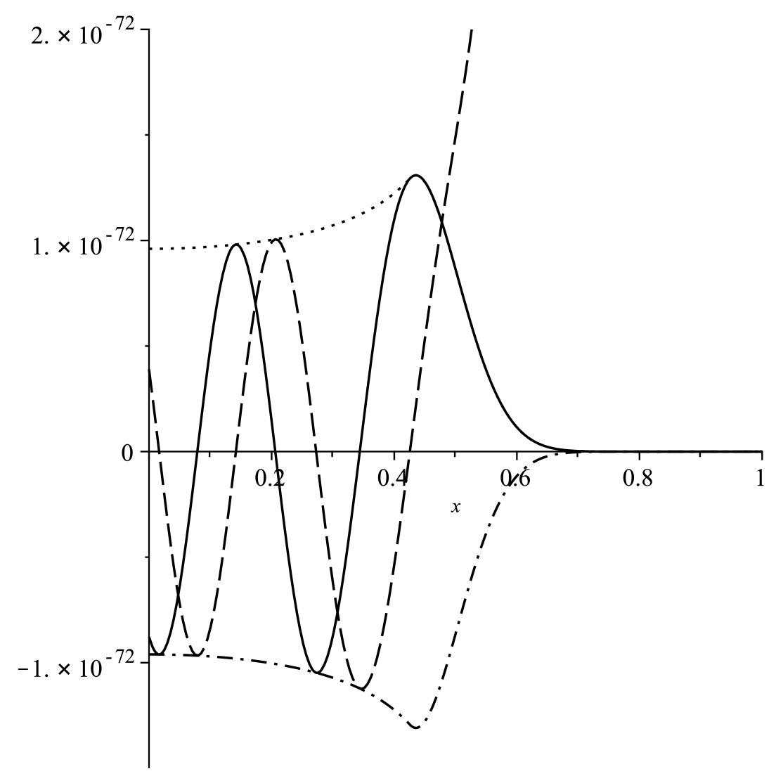
Figure 3: Graphs of $\mathsf{P}^{-\mu}_{\nu}(x)$ (solid curve), $2\mathsf{Q}^{-\mu}_{\nu}(x)/\pi$ (dashed curve), $M(\nu,\mu,x)$ (dotted curve) and $-M(\nu,\mu,x)$ (dash-dotted curve) for $\nu=50$ and $\mu=(1-a^{2})^{1/2}u$ ($u=\nu+\frac{1}{2}$) with $a=0.5$.

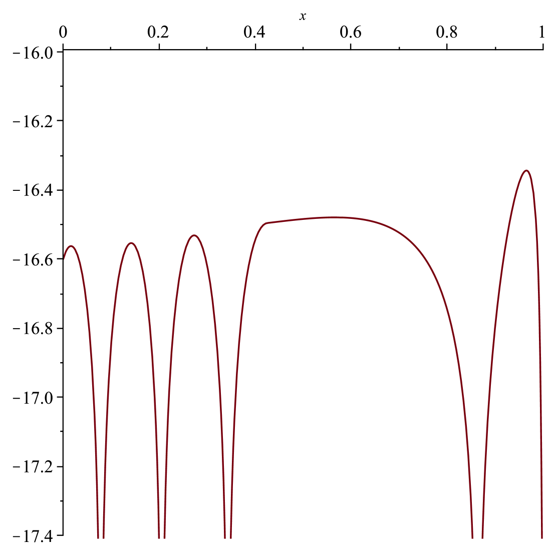
Figure 4: Graph of $\Omega_{4}(\nu,\mu,x)$ for $\nu=50$ and $\mu=(1-a^{2})^{1/2}u$ ($u=\nu+\frac{1}{2}$), with $a=0.5$.

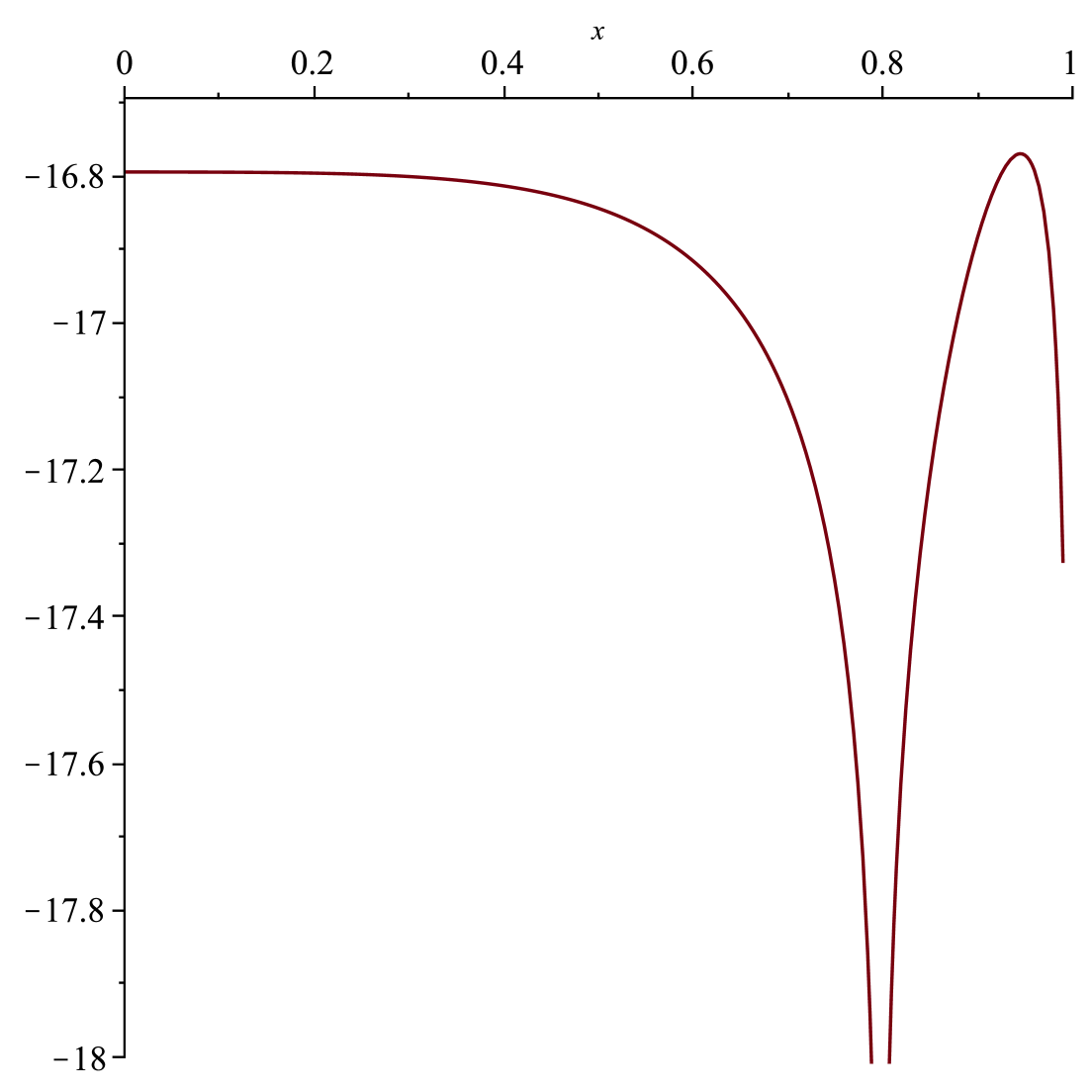
Figure 5: Graph of $\Omega_{4}(\nu,\mu,x)$ for $\nu=50$ and $\mu=(1-a^{2})^{1/2}u$ ($u=\nu+\frac{1}{2}$), with $a=0.1$.

Next, for $z=x\in[0,1)$, on taking the first four terms in Eqs. 182, 183, 184, and 185 define the approximations

(195) $$\mathcal{A}_{4}(u,a,x)=\frac{\pi^{1/4}}{u^{1/4}\sqrt{2\Gamma(u+\mu+\tfrac{1}{2})}}\left(\frac{\zeta^{2}-\alpha^{2}}{x^{2}-a^{2}}\right)^{1/4}\left\{1+\sum_{s=1}^{3}\frac{\mathrm{A}_{s}(a,x)}{u^{2s}}\right\},$$

and

(196) $$\mathcal{B}_{4}(u,a,x)=\frac{\pi^{1/4}}{u^{1/4}\sqrt{2\Gamma(u+\mu+\tfrac{1}{2})}}\left(\frac{\zeta^{2}-\alpha^{2}}{x^{2}-a^{2}}\right)^{1/4}\sum_{s=0}^{3}\frac{\mathrm{B}_{s}(a,x)}{u^{2s+2}},$$

where $\zeta=\zeta(x)\in[0,\infty)$ is given by Eqs. 156 and 157. Then from Eqs. 160, 195, and 196 consider the following error for $z=x\in[0,1)$ in the approximation

(197) $$\Delta_{4}(\nu,\mu,x)=\mathsf{P}^{-\mu}_{\nu}(x)-\sqrt{\frac{2}{\pi}}\Biggl{\{}U\left(\mu-\nu-\tfrac{1}{2},\sqrt{2u}\,\zeta\right)\mathcal{A}_{4}(u,a,x)\Biggr{.}\\ \left.+\frac{\partial U\left(\mu-\nu-\tfrac{1}{2},\sqrt{2u}\,\zeta\right)}{\partial\zeta}\mathcal{B}_{4}(u,a,x)\right\}.$$

To assess the relative accuracy of this, we computed

(198) $$\Omega_{4}(\nu,\mu,x)=\log_{10}\left\{\frac{\left|\Delta_{4}(\nu,\mu,x)\right|}{M(\nu,\mu,x)}\right\}\quad(0\leq x<1).$$

A plot of $\Omega_{4}(\nu,\mu,x)$ with $\nu=50$ ($u=101/2$) and $\mu=(1-a^{2})^{1/2}u$ is given in Fig. 4 for $a=0.5$, and in Fig. 5 for $a=0.1$. In the latter case $\mathsf{P}^{-\mu}_{\nu}(z)$ does not have zeros in $[0,1)$ and so we took $M(\nu,\mu,x)=\mathsf{P}^{-\mu}_{\nu}(z)$ in (198).

In both cases, we used the Taylor series about $x=a$ for $|x-a|<0.08$ as described above (see Eq. 193), and computed the coefficients in Eqs. 195 and 196 directly for all other values of $x$. The plots demonstrate about 16 digits, or better, of accuracy for both values of $a$, uniformly throughout the interval.

Conflict of interest

The author has no conflict of interest to declare that is relevant to the content of this article.

References

[1]T. Barakat, The asymptotic iteration method for the eigenenergies of the anharmonic oscillator potential , Phys. Lett. A., 344 (2005), pp. 411–417, https://doi.org/10.1016/j.physleta.2005.06.081.
[2]W. G. C. Boyd and T. M. Dunster, Uniform asymptotic solutions of a class of second-order linear differential equations having a turning point and a regular singularity, with an application to Legendre functions, SIAM J. Math. Anal., 17 (1986), pp. 422–450, https://doi.org/10.1137/0517033.
[3]NIST Digital Library of Mathematical Functions.
Release 1.1.6 of 2022-06-30, http://dlmf.nist.gov/.
F. W. J. Olver, A. B. Olde Daalhuis, D. W. Lozier, B. I. Schneider, R. F. Boisvert, C. W. Clark, B. R. Miller, B. V. Saunders, H. S. Cohl, and M. A. McClain, eds.
[4]T. M. Dunster, Liouville-Green expansions of exponential form, with an application to modified Bessel functions, Proc. Roy. Soc. Edinburgh Sec. A, 150 (2020), pp. 1289–1311, https://doi.org/10.1017/prm.2018.117.
[5]T. M. Dunster, Nield-Kuznetsov functions and Laplace transforms of parabolic cylinder functions, SIAM J. Math. Anal., 53 (2021), pp. 5915–5947, https://doi.org/10.1137/21M1401590.
[6]T. M. Dunster, A. Gil, and J. Segura, Computation of asymptotic expansions of turning point problems via Cauchy’s integral formula: Bessel functions, Constr. Approx., 46 (2017), pp. 645–675, https://doi.org/10.1007/s00365-017-9372-8.
[7]T. M. Dunster, A. Gil, and J. Segura, Simplified error bounds for turning point expansions, Anal. Appl., 19 (2021), pp. 647–678, https://doi.org/10.1142/S0219530520500104.
[8]H. Ezawa, T. Nakamura, K. Watanabe, and T. Irisawa, Convergent iteration method for the anharmonic oscillator Schrödinger eigenvalue problem, J. Phys. Soc. Jpn., 81 (2012), https://doi.org/10.1143/JPSJ.81.034003.
[10]N. D. Kazarinoff, Asymptotic theory of second order differential equations with two simple turning points, Arch. Rational Mech. Anal., 2 (1958), pp. 129–150, https://doi.org/10.1007/BF00277924.
[11]R. E. Langer, The asymptotic solutions of certain linear ordinary differential equations of the second order, Trans. Amer. Math. Soc., 36 (1934), p. 90–106, https://doi.org/10.1090/S0002-9947-1934-1501736-5.
[12]R. E. Langer, The asymptotic solutions of a linear differential equation of the second order with two turning points, Trans. Amer. Math. Soc., 90 (1959), pp. 113–142, https://doi.org/10.1090/S0002-9947-1959-0105530-9.
[13]R. Y. S. Lynn and J. B. Keller, Uniform asymptotic solutions of second order linear ordinary differential equations with turning points, Commun. Pure Appl. Math., 23 (1970), pp. 379–408, https://doi.org/10.1002/cpa.3160230310.
[14]R. W. McKelvey, The solutions of second order linear ordinary differential equations about a turning point of order two, Trans. Amer. Math. Soc., 79 (1955), pp. 103–123, https://doi.org/10.1090/S0002-9947-1955-0069344-7.
[15]H. Moriguchi, An improvement of the WKB method in the presence of turning points and the asymptotic solutions of a class of Hill equations, J. Phys. Soc. Jpn., 14 (1959), pp. 1771–1796, https://doi.org/doi:10.1143/JPSJ.14.1771.
[16]F. W. J. Olver, Legendre functions with both parameters large, Philos. Trans. Roy. Soc. London Ser. A, 278 (1975), pp. 175–185, https://doi.org/10.1098/rsta.1975.0024.
[17]F. W. J. Olver, Second-order linear differential equations with two turning points, Philos. Trans. Roy. Soc. London Ser. A, 278 (1975), pp. 137–174, https://doi.org/10.1098/rsta.1975.0023.
[19]F. W. J. Olver, Asymptotics and special functions, AKP Classics, A K Peters Ltd., Wellesley, MA, 1997.
Reprint of the 1974 original [Academic Press, New York].