Ridge partial correlation screening for ultrahigh-dimensional data

Abstract

Variable selection in ultrahigh-dimensional linear regression is challenging due to its high computational cost. Therefore, a screening step is usually conducted before variable selection to significantly reduce the dimension. Here we propose a novel and simple screening method based on ordering the absolute sample ridge partial correlations. The proposed method takes into account not only the ridge regularized estimates of the regression coefficients but also the ridge regularized partial variances of the predictor variables providing sure screening property without strong assumptions on the marginal correlations. Simulation study and a real data analysis show that the proposed method has a competitive performance compared with the existing screening procedures. A publicly available software implementing the proposed screening accompanies the article.

Key words: Feature selection; High dimensional ordinary least squares projection (HOLP); Large $p$ small $n$; $q$-exponential tail; Screening consistency; Sure independent screening

1 Introduction

In recent years, data sets with hundreds of thousands of variables are more and more common in diverse disciplines– agronomy, biology, engineering, genomics, medicine, and the list goes on and on. Nevertheless, the number of variables which cause significant impact on the response are relatively small. For example, only a handful of genes are known to directly associate with Type 1 diabetes among a host of genes. Thus, variable selection methods have been attracting researchers’ attention and in the past several years, we have witnessed a lot of research results appearing in this area. A widely used approach to perform variable selection and coefficient estimation simultaneously is by penalizing a loss function to get a shrinkage estimator of the coefficient. This class of methods include the popular lasso [Tibshirani, 1996], the elastic net [Zou and Hastie, 2005], the SCAD [Fan and Li, 2001], the adaptive lasso [Zou, 2006], the ridge regression [Hoerl and Kennard, 1970] , and the bridge regression [Huang et al., 2008].

In ultrahigh-dimensional settings, the number of variables $p$ far exceeds the number of observations $n$. In such $p\gg n$ settings, the shrinkage methods may fail and the computational cost for the corresponding large-scale optimization problem is not ignorable. Thus, the feature screening methods, which aim to reduce the large dimensionality rapidly and efficiently, are performed in this setting before conducting a refined model selection analysis. Motivated by these, Fan and Lv [2008] introduced the sure independence screening (SIS) method in which the $n$ variables with the largest marginal (Pearson) correlations with the response survive after screening. The SIS method is then extended to generalized linear models [Fan and Song, 2010], additive models [Fan et al., 2011], and the proportional hazards model [Zhao and Li, 2012, Gorst-Rasmussen and Scheike, 2013]. Although SIS method can reduce the dimension rapidly to a manageable size, it is showed in Wang et al. [2021] that SIS may fail in the presence of correlated predictors. Based on Fan and Lv’s [2008] work, several other correlation measures such as general correlation [Hall and Miller, 2009], distance correlation [Li et al., 2012b], rank correlation [Li et al., 2012a], tilted correlation [Cho and Fryzlewicz, 2012, Lin and Pang, 2014] and quantile partial correlation [Ma et al., 2017] have also been proposed as variable screening tools. Other variable screening methods include the traditional forward regression (FR) method [Wang, 2009] [see also Hao and Zhang, 2014] and high dimensional ordinary least squares projection (HOLP) [Wang and Leng, 2016].

In this paper, we propose a novel variable screening method based on the ridge partial correlation (RPC). This method is motivated by the Bayesian iterated screening (BITS) of Wang et al. [2025] who introduced the ridge partial correlation to demonstrate contrasts of BITS with FR. The proposed RPC screening method makes use of the partial correlation information as well as the shrinkage effect due to the ridge penalty. Given the response $y$ and the predictors $(x_{1},x_{2},\dots,x_{p})$, the partial correlation of $x_{i}$ and $y$ is the correlation between $x_{i}$ and $y$ controlling the effect of all other predictors $(x_{1},\dots,x_{i-1},x_{i+1},x_{p})$. This property is inherited by RPC. Thus, the RPC screening will not likely select the unimportant variables that are correlated with the important variables, which is not the case with the SIS. The implementation of the RPC screening is straightforward and efficient by a parallel computing algorithm proposed here. We prove that, asymptotically, RPC screening has the same path as the HOLP and thus RPC has the sure screening property. We show that, like the HOLP method, RPC has screening consistency under the general $q$-exponential tail condition on the errors and it does not require the marginal correlations for the important variables to be bounded away from zero—an impractical assumption used for showing screening consistency of SIS. Thus, RPC satisfies the two important aspects of a successful screening method mentioned in Wang and Leng [2016], namely the computational efficiency and the screening consistency property under flexible conditions. Moreover, although RPC has similarities with the HOLP, unlike HOLP, RPC takes into account (ridge) partial variances of the variables, and numerical examples show that RPC can lead to better performance than the HOLP and other variable screening methods.

The rest of the paper is organized as follows. We describe the RPC screening method in Section 2. The screening consistency property is discussed and established in Section 2.3. In Section 3, we propose a fast statistical computation algorithm for RPC screening. Section 4 includes results from an extensive simulation study. A real data set involving a mammalian eye disease study is analyzed in Section 5. Section 6 contains a short discussion. Several theoretical results, proofs of the theorems and additional simulation results are given in the supplement. The methodology proposed here is implemented in an accompanying R package rpc [Dutta and Nguyen, 2025].

2 Ridge partial correlation screening method

2.1 Linear regression model

Consider the familiar linear regression model

$$y=\beta_{0}+\beta_{1}x_{1}+\beta_{2}x_{2}+\ldots+\beta_{p}x_{p}+\epsilon$$ (1)

where $y$ is the response, $x=(x_{1},\dots,x_{p})^{\top}$ is the random vector of predictors, $\beta_{0}\in\mathcal{R}$ is the intercept, $\beta=(\beta_{1},\dots,\beta_{p})\in\mathcal{R}^{p}$ is the vector of regression coefficients, and $\epsilon$ is the random error. We also write the model (1) corresponding to $n$ realizations of $(x,y)$ as

$$Y=\beta_{0}1_{n}+X\beta+\varepsilon,$$ (2)

where $Y$ is the $n\times 1$ vector of response values, $1_{n}$ is the $n\times 1$ vector with all entries equal to 1, $X$ is the $n\times p$ design matrix, and $\varepsilon\in\mathcal{R}^{n}$ is the vector consisting of identically and independently distributed residual errors with mean zero and variance $\sigma^{2}$.

2.2 The ridge partial correlation screening method

Partial correlation measures the correlation between two variables when conditioned on other variables. The marginal correlation based screening methods like SIS [Fan and Lv, 2008] suffer from the problem that unimportant variables those are marginally correlated with important variables may get selected [Wang et al., 2021]. Replacing marginal correlation with partial correlation a screening method helps to solve this problem as partial correlation removes the effects of conditioned variables. The (population) partial correlation between the $i$th predictor variable $x_{i}$ and the response $y$ given the remaining predictor variables is the negative of the $(1,i)$th entry of the correlation matrix corresponding to $\tilde{\Sigma}^{-1}$ where $\tilde{\Sigma}$ is the covariance matrix of the random vector $(y,x)$. We assume that the $p$ columns of the matrix $X$ are centered and scaled. If $p/n\to 0$, a consistent estimator of $\tilde{\Sigma}^{-1}$ is given by

$$n\begin{pmatrix}\tilde{Y}^{\top}\tilde{Y}&\tilde{Y}^{\top}X\\ X^{\top}\tilde{Y}&X^{\top}X\end{pmatrix}^{-1},$$ (3)

where $\tilde{Y}=Y-\bar{Y}1_{n},$ and $\bar{Y}=1_{n}^{\top}Y/n$ is the average of the responses. However, if $p>n$, the inverse of the matrix in (3) is not defined. This motivated us to consider the ridge regularized estimator of $\tilde{\Sigma}^{-1}$ given by $\bm{R}$, where

$$\bm{R}:=n\begin{pmatrix}\tilde{Y}^{\top}\tilde{Y}&\tilde{Y}^{\top}X\\ X^{\top}\tilde{Y}&X^{\top}X+\lambda I\end{pmatrix}^{-1},$$ (4)

and $I$ is the identity matrix. Note that, in (4), the predictor variables have been penalized while the response variable is not. We now describe our proposed screening method. This method uses the sample ridge partial correlation between $x_{i}$ and $y$ as defined below.

Definition 1.

For any $i$, the sample ridge partial correlation between $y$ and $x_{i}$ with ridge penalty $\lambda$ is given by

$$R_{i,\lambda}=-v_{iy,\lambda}/\{v_{i,\lambda}\times v_{y,\lambda}\}^{1/2},$$ (5)

where $v_{iy,\lambda}$ is the $(1,i+1)$th element of $\bm{R}$, $v_{i,\lambda}$ is the $(i+1,i+1)$th diagonal element of $\bm{R}$, and $v_{y,\lambda}$ is the $(1,1)th$ element of $\bm{R}$.

For variable screening, we rank the absolute sample ridge partial correlations and select the $K$ variables with the largest (absolute) ridge partial correlations. More specifically, let $K$ be the number of variables survived after screening. Then, given the ridge penalty $\lambda$, we choose the submodel $\gamma^{K}\subseteq\{1,2,\ldots,p\}$ as

$$\gamma^{K}=\{i:|R_{i,\lambda}|\text{ is among the largest $K$ of all $|R_{i,\lambda}|$'s}\}.$$

Note that, Wang and Leng’s [2016] HOLP procedure chooses the variables based on the ridge estimator of $\beta_{i}$’s, that is, based on $|v_{iy,\lambda}|$ values. Whereas, the ridge partial correlation also takes into account the (ridge) partial variances $v_{i,\lambda}$’s of the $i$th variable given the rest of the predictor variables and the response. Thus, between two candidates with the same (absolute ridge) regression coefficient estimate, the one with the smaller partial variance is preferred. In different simulation examples in Section 4, we demonstrate that RPC can perform better than HOLP.

2.3 Screening consistency

In order to state the assumptions and the theoretical results, we use the following notations. For two real sequences $\{a_{n}\}$ and $\{b_{n}\}$, $a_{n}\sim b_{n}$ means ${a_{n}}/{b_{n}}\rightarrow c$ for some constant $c>0$; $a_{n}\succeq b_{n}$ (or $b_{n}\preceq a_{n}$) means $b_{n}=O(a_{n})$; $a_{n}\succ b_{n}$ (or $b_{n}\prec a_{n}$) means $b_{n}=o(a_{n})$. Also, for any matrix $A$, let $\alpha_{min}(A)$ and $\alpha_{max}(A)$ denote its minimum and maximum eigenvalues, respectively, and let $\alpha_{min}^{*}(A)$ be its minimum nonzero eigenvalue. Finally, for a positive definite matrix $A$, let $\text{cond}(A)=\alpha_{max}(A)/\alpha_{min}(A)$ denotes the condition number of $A$.

Recall that $X$ denotes the design matrix. Assume that the rows of $X$ are identically and independently distributed with zero mean vector and covariance matrix $\Sigma$. That is, $\Sigma=$ cov $(x)$ is the covariance matrix of the predictors. Define $Z=X\Sigma^{-1/2}$ and $z=\Sigma^{-1/2}x$. For simplicity, as in Wang and Leng [2016], we assume that all diagonal entries of $\Sigma$ are equal to one, that is, $\Sigma$ is the correlation matrix.

Performance of a screening method crucially depends on the tail behavior of the errors $\varepsilon$. Screening consistency of HOLP and BITS has been established in Wang and Leng [2016] and Wang et al. [2025], respectively under the below mentioned general $q-$exponential tail condition of the errors.

Definition 2 ($q$-exponential tail condition).

A zero-mean distribution $F$ is said to have $q$-exponential tail, if there exists a function $q:[0,\infty)\to\mathbb{R}$ such that for any $N\geq 1,$ $\eta_{1},\ldots,\eta_{N}\stackrel{{\scriptstyle iid}}{{\sim}}F$, $\ell\in{\cal R}^{N}$ with $\|\ell\|=1$, and $\zeta>0$ we have $P\left(\left|\ell^{\top}\eta\right|>\zeta\right)\leq\exp\{1-q(\zeta)\}$ where $\eta=(\eta_{1},\ldots,\eta_{N})^{\top}.$

As shown in Vershynin [2012], for the standard normal distribution, $q(\zeta)=\zeta^{2}/2,$ when $F$ is sub-Gaussian $q(\zeta)=c_{F}\zeta^{2}$ for some constant $c_{F}>0$ depending on $F,$ and when $F$ is sub-exponential distribution $q(\zeta)=c^{\prime}_{F}\zeta$ for some constant $c^{\prime}_{F}>0$ depending on $F.$ Finally, if only first $2k$ moments of $F$ are finite, then $q(\zeta)-2k\log(\zeta)=O(1).$

For a subset $\gamma\subset\{1,2,\dots,p\}$, let $|\gamma|$ be the cardinality of $\gamma$ and $X_{\gamma}$ be the $n\times|\gamma|$ submatrix of $X$ consisting of the columns of $X$ corresponding $\gamma$. We make the following set of assumptions:

• $Y=\beta_{0}1_{n}+X_{t}\beta_{t}+\varepsilon$ where $t$ is the true model for some subset $t\subset\{1,2,\dots,p\}$, $\varepsilon=(\varepsilon_{1},\dots,\varepsilon_{n}),$ $\varepsilon_{i}/\sigma\stackrel{{\scriptstyle iid}}{{\sim}}F_{0}$ which has $q$-exponential tail with unit standard deviation.

• $z$ has a spherically symmetric distribution and there are some constants $c_{1}>1$ and $C_{1}>0$ such that

  $$P\{\alpha_{\max}(p^{-1}ZZ^{\top})>c_{1}\text{ or }\alpha_{\min}(p^{-1}ZZ^{\top})<c_{1}^{-1})\}\leq\exp(-C_{1}n).$$

• We assume that $\text{var}(y)=O(1)$ and that, for some $\kappa\geq 0,\nu\geq 0,\tau\geq 0$ and $c_{2},c_{3},c_{4}>0$ independent of $n,p$,

  $$\min_{j\in t}|\beta_{j}|\geq\dfrac{c_{2}}{n^{\kappa}},\qquad|t|\leq c_{3}n^{\nu}\quad\text{and}\quad\text{cond}(\Sigma)\leq c_{4}n^{\tau}.$$

• Finally, we assume

  $$p\succ n^{1+\tau},\quad\log(p)\prec\min\left\{\dfrac{n^{1-2\kappa-5\tau}}{2\log(n)},q\left(\dfrac{\sqrt{C_{1}}n^{1/2-2\tau-\kappa}}{\sqrt{\log(n)}}\right)\right\}$$

  and $\lambda\prec n^{1-(5/2)\tau-\kappa}$.

The conditions A1–A3 as well as the second condition on $p$ in the assumption A4 are also assumed in Wang and Leng [2016] for proving screening consistency of the HOLP. Let $S_{\lambda}=\tilde{Y}^{\top}\tilde{Y}-\tilde{Y}^{\top}X(X^{\top}X+\lambda I)^{-1}X^{\top}\tilde{Y}=n/v_{y,\lambda}$ be the ridge residual sum of squares. The screening consistency result for the RPC method is stated in the following theorem.

Theorem 1.

Under the assumptions A1–A4, there exists $\rho_{n}$ (defined in Appendix S3) such that

$$\begin{split}P\bigg{(}\min_{i\in t}R_{i,\lambda}^{2}>\dfrac{\rho_{n}^{2}}{S_{\lambda}+\rho_{n}^{2}}>\max_{i\notin t}R_{i,\lambda}^{2}\bigg{)}&=1-O\bigg{(}\exp\bigg{\{}-C_{1}\dfrac{n^{1-5\tau-2\kappa-\nu}}{2\log(n)}\bigg{\}}\\ &+\exp\bigg{[}1-\dfrac{1}{2}q\bigg{\{}\dfrac{\sqrt{C_{1}}n^{1/2-2\tau-\kappa}}{\sqrt{\log(n)}}\bigg{\}}\bigg{]}\bigg{)}.\end{split}$$

Alternatively, there exist $K_{n}\sim n^{\iota}$ for some $\iota\in(\nu,1]$ such that

$$P(t\subset\gamma^{K_{n}})=1-O\left(\exp\left\{-C_{1}\dfrac{n^{1-2\kappa-5\tau-\nu}}{2\log(n)}\right\}+\exp\left[1-\dfrac{1}{2}q\left(\dfrac{\sqrt{C_{1}}n^{1/2-2\tau-\kappa}}{\sqrt{\log(n)}}\right)\right]\right)$$

Proof.

The proof of the theorem is given in Section S3 of the supplement. ∎

The second result, which directly follows from the first result, reveals that, if a submodel of size larger than the true model is selected, then the submodel contains the true model with probability tending to one.

3 Fast statistical computation

In this section we describe how the ridge partial correlation coefficients are computed at the same order of computing cost as HOLP. To that end, let $W=XX^{\top}+\lambda I.$ Then, using Woodbury matrix identity,

$$\begin{split}v_{y,\lambda}/n&=(\tilde{y}^{\top}\tilde{y}-\tilde{y}^{\top}X(X^{\top}X+\lambda I)^{-1}X^{\top}\tilde{y})^{-1}\\ &=(\tilde{y}^{\top}\tilde{y}-\tilde{y}^{\top}X\left\{\dfrac{1}{\lambda}I-\dfrac{1}{\lambda}X^{\top}(XX^{\top}+\lambda I)^{-1}X\right\}X^{\top}\tilde{y})^{-1}\\ &=(\tilde{y}^{\top}\tilde{y}-\dfrac{1}{\lambda}\tilde{y}^{\top}XX^{\top}\tilde{y}+\dfrac{1}{\lambda}\tilde{y}^{\top}XX^{\top}(XX^{\top}+\lambda I)^{-1}XX^{\top}\tilde{y})^{-1}\\ &=(\tilde{y}^{\top}\tilde{y}-\dfrac{1}{\lambda}\tilde{y}^{\top}XX^{\top}\tilde{y}+\dfrac{1}{\lambda}\tilde{y}^{\top}XX^{\top}\tilde{y}-\tilde{y}^{\top}(XX^{\top}+\lambda I)^{-1}XX^{\top}\tilde{y})^{-1}\\ &=(\tilde{y}^{\top}\tilde{y}-\tilde{y}^{\top}\tilde{y}+\lambda\tilde{y}^{\top}(XX^{\top}+\lambda I)^{-1}\tilde{y})^{-1}\\ &=1/\left[\lambda\tilde{y}^{\top}W^{-1}\tilde{y}\right].\end{split}$$ (6)

Similarly, if $e_{i}$ denotes the $i$th canonical basis vector of $\mathbb{R}^{p},$ then,

$$\begin{split}v_{iy,\lambda}/n&=-e_{i}^{\top}(X^{\top}X+\lambda I)^{-1}X^{\top}\tilde{y}~/~\left[\tilde{y}^{\top}\tilde{y}-\tilde{y}^{\top}X(X^{\top}X+\lambda I)^{-1}X^{\top}\tilde{y}\right]\\ &=-X^{\top}_{i}W^{-1}\tilde{y}/\left[\lambda\tilde{y}^{\top}W^{-1}\tilde{y}\right],\end{split}$$ (7)

and finally,

$$\begin{split}v_{i,\lambda}/n&=e_{i}^{\top}\left\{(X^{\top}X+\lambda I)^{-1}+\dfrac{(X^{\top}X+\lambda I)^{-1}X^{\top}\tilde{y}\tilde{y}^{\top}X(X^{\top}X+\lambda I)^{-1}}{\tilde{y}^{\top}\tilde{y}-\tilde{y}^{\top}X(X^{\top}X+\lambda I)^{-1}X^{\top}\tilde{y}}\right\}e_{i}\\ &=e_{i}^{\top}\left\{\dfrac{1}{\lambda}I-\dfrac{1}{\lambda}X^{\top}(XX^{\top}+\lambda I)^{-1}X\right\}e_{i}+\dfrac{(X^{\top}_{i}W^{-1}\tilde{y})^{2}}{\lambda\tilde{y}^{\top}W^{-1}\tilde{y}}\\ &=\dfrac{1}{\lambda}+\dfrac{(X^{\top}_{i}W^{-1}\tilde{y})^{2}}{\lambda\tilde{y}^{\top}W^{-1}\tilde{y}}-\dfrac{1}{\lambda}X^{\top}_{i}W^{-1}X_{i}\end{split}$$ (8)

3.1 Algorithm for computing ridge partial correlations

In practice, these quantities can be efficiently computed using the Cholesky factor of $W$: Let $S$ be an upper triangular matrix such that $W=S^{\top}S$. Let $\theta=S^{-\top}\tilde{y},u_{i}=S^{-\top}X_{i}$. Then $\tilde{y}^{\top}W^{-1}\tilde{y}=\theta^{\top}\theta,X^{\top}_{i}W^{-1}\tilde{y}=u^{\top}_{i}\theta$ and $X^{\top}_{i}W^{-1}X_{i}=u^{\top}_{i}u_{i}$. Substitute these equations into (6), (7) and (8), we get the following algorithm for computing ridge partial correlations:

1. Given $X,\tilde{y}$ and $\lambda$, compute $W=XX^{\top}+\lambda I$.

2. Compute the Cholesky factor of $W$, denoted by $S$, which is upper triangular satisfying $W=S^{\top}S$.

3. Compute $\theta=S^{-\top}\tilde{y}$ and $v_{y,\lambda}=n/(\lambda\theta^{\top}\theta).$

4. For each $i=1,2,\ldots,p$,

   • compute $u_{i}=S^{-\top}X_{i}$, $v_{iy,\lambda}=-v_{y,\lambda}\cdot u_{i}^{\top}\theta$ and $v_{i,\lambda}=n\lambda^{-1}+v_{y,\lambda}(u_{i}^{\top}\theta)^{2}-n\lambda^{-1}u^{\top}_{i}u_{i}.$

   • Compute $R_{i,\lambda}=-v_{iy,\lambda}/\{v_{i,\lambda}\times v_{y,\lambda}\}^{1/2}$

In the above algorithm, the third step can be parallelized over $i$ as implemented in the R package rpc [Dutta and Nguyen, 2025]. Overall, the computational complexity of the above algorithm is $O(n^{3})+O(n^{2}p)$ where the $O(n^{3})$ term correspond to computing the Cholesky factorization of $XX^{\top}+\lambda I_{n}$ and the $O(n^{2}p)$ term arises due to computing $XX^{\top}$ and for computing $u_{i}$s. This is encouragingly the same as the computational complexity of HOLP.

4 Simulation study

In this section, we compare the performance of the proposed ridge partial correlation screening with SIS (Fan and Lv [2008]), forward regression (Wang [2009]), BITS (Wang et al. [2025]) and HOLP (Wang and Leng [2016]) by extensive simulation studies.

4.1 Simulation settings

We consider seven data generating models in our numerical studies. For these settings E.1–E.7, the rows of $X$ are generated from multivariate normal distributions with mean zero and different covariance structures. We consider $n=300$ and $p=5000$ in all simulation settings. The response variable $y$ is generated by model (1) with error term $\epsilon$ following three separate distributions with different tail behaviors. In the first case, we consider $\epsilon$ to be normally distributed with mean 0 and variance 1. Next, we take $\epsilon$ to be shifted exponentially distributed with mean 0 and variance 1 and support $[-1,\infty)$, that is, $\epsilon\stackrel{{\scriptstyle d}}{{=}}\zeta-1$ where $\zeta\sim\text{Exp}(1)$. Finally, we consider $\epsilon$ to be scaled student $t$ distributed with degrees of freedom 20, mean 0 and variance 1, that is, $\epsilon\stackrel{{\scriptstyle d}}{{=}}\eta/\sqrt{20/18}$ where $\eta\sim t_{20}$. Four values of theoretical $R^{2}(=$ Var $(x^{\top}\beta)/$ Var $(y))$, namely $R^{2}=0.1,0.2,0.3,$ and $0.4$ are assumed. In E.1 - E.6, $\beta_{j}=1$ for $j\leq 9$ and $\beta_{j}=0$ for $j>9$. In E.7, $\beta_{j}=1$ for $j\leq 25$ and $\beta_{j}=0$ for $j>25$.

1. Independent predictors    In this example, $\Sigma=I_{p},$ the identity matrix of dimension $p$.

2. Compound symmetry    Here, $\Sigma=\rho 1_{p}1_{p}^{\top}+(1-\rho)I_{p}.$ We set $\rho=0.5$ in our study.

3. Autoregressive correlation    This correlation structure is appropriate if there is an ordering (say, based on time) in the covariates, and variables further apart are less correlated. We use the AR(1) structure where the $(i,j)$th entry of $\Sigma$ is $\rho^{|i-j|}.$ We set $\rho=0.5$ in our study.

4. Factor models    This example is from Wang and Leng [2016]. Fix $k=10.$ Let $F$ be a $p\times k$ random matrix with entries iid $\mathcal{N}(0,1).$ The $\Sigma$ is then given by $FF^{\top}+I_{p}.$

5. Group structure    In this example, the true variables in the same group are highly correlated. This is a modification of example 4 of Zou and Hastie [2005]. The predictors are generated by $X_{m}=z_{1}+\zeta_{1,m}$, $X_{3+m}=z_{2}+\zeta_{2,m}$, $X_{6+m}=z_{3}+\zeta_{3,m}$ where $z_{i}\overset{iid}{\sim}{\cal N}_{n}(0,I_{n})$, $\zeta_{i,m}\overset{iid}{\sim}{\cal N}_{n}(0,0.01I_{n})$ and $z_{i}$’s and $\zeta_{i,m}$’s are independent for $1\leq i\leq 3$ and for $m=1,2,3$.

6. Extreme correlation    This example is a modification of the challenging example 4 of Wang [2009], making it more complex. Generate $Z_{i}\stackrel{{\scriptstyle iid}}{{\sim}}{\cal N}_{n}(0,I),i=1,\dots,p$, and $W_{i}\stackrel{{\scriptstyle iid}}{{\sim}}{\cal N}_{n}(0,I),i=1,\dots,9$. Set $X_{i}=(Z_{i}+W_{i})/\sqrt{2},i=1,\dots,9$ and $X_{i}=(Z_{i}+\sum_{i=1}^{9}W_{i})/2$ for $i=10,\dots,p$. The marginal correlation between $y$ and $X_{i},i\geq 10$ (unimportant variables) is $2.5/\sqrt{3}$ times larger than the same between $y$ and $X_{j},j\leq 9$ (important variables).

7. Sparse factor models    This is the sparse version of E.4. For each $1\leq j\leq 5,$ generate $f_{ij}\sim{\cal N}(0,1)$ if $5(j-1)+1\leq i\leq 5j,$ and $f_{ij}=0$ otherwise. Also, $\Sigma=FF^{\top}+0.01I_{p}.$

For each simulation setup, a total of 100 data sets are generated and we evaluate the performance of each method by the coverage probability (CP) and true positive rate (TPR). The CP and TPR are defined as follows. Let $\hat{\gamma}^{(i)}$ denote the chosen model in the $i$th replication for $i=1,2,\ldots,100.$ The coverage probability is calculated by CP = $\sum_{i=1}^{100}\mathbb{I}(\widehat{\gamma}^{(i)}\supseteq t)/100$. The true positive rate is calculated by TPR = $(1/100)\sum_{i=1}^{100}\big{|}\widehat{\gamma}^{(i)}\cap t\big{|}/|t|.$ The CP measures whether all the important variables are survived after screening while TPR measures how many important variables are survived after screening.

4.2 Summary of simulation results

The simulation results for $R^{2}=0.2$ and normally distributed errors are shown in Table 1. Three distinct values of $\lambda$, namely $p/n$ (RPC1), $n\log n/p$ (RPC2) and $n/p$ (RPC3) are considered in our study. All these three methods select a submodel of size $n$. The URPC selects the union of submodels given by RPC1, RPC2 and RPC3. The UBITS selects the union of submodels of size $n$ given by BITS with the same three choices of $\lambda$ as RPC1, RPC2, and RPC3, respectively.

In general, the RPC method is not sensitive to the value of $\lambda$. In most cases, the RPC method leads to similar performance as the HOLP and is competitive with the other methods. However, in the most difficult case of extreme correlation E.6, RPC beats all other methods, including the HOLP. Surprisingly, the RPC methods have almost twice coverage probability than the HOLP in the setup E.6. Therefore, despite having some similarities with the HOLP, RPC provides better performance than the HOLP.

Results from the other simulation settings corresponding to different $R^{2}$ values, and other error distributions are provided in Section S4 of the supplement.

Table 1: Simulation results (in %) for $R^{2}=0.2$ and error normally distributed.

Method	Correlation Structure
	IID		Compound		Group		AR		Factor		ExtrCor		SpFactor
	TPR	CP	TPR	CP	TPR	CP	TPR	CP	TPR	CP	TPR	CP	TPR	CP
RPC1	75.6	9	16.8	0	98.3	92	95.6	69	14.8	0	82.8	17	55.9	0
RPC2	75.6	9	16.8	0	98.3	92	95.6	69	15.1	0	82.8	19	56.0	0
RPC3	75.6	9	16.8	0	98.3	92	95.6	69	14.8	0	82.8	17	55.9	0
URPC	75.6	9	16.8	0	98.3	92	95.6	69	15.1	0	83.0	19	56.0	0
UBITS	74.3	9	22.8	0	98.3	94	91.7	44	23.0	0	35.7	0	70.0	1
HOLP	75.6	9	16.9	0	98.3	92	95.6	69	14.9	0	77.4	10	56.0	0
FR	32.1	0	7.7	0	34.2	0	34.1	0	7.3	0	12.2	0	13.6	0
SIS	77.4	11	23.8	0	99.6	98	97.3	80	20.1	0	0.4	0	62.5	1

5 Real data application

Bai et al. [2022] analyzed a mammalian eye disease data set where gene expression measurements on the eye tissues from 120 female rats were recorded. This data set was originally analyzed by Scheetz et al. [2006]. In this data set, the gene TRIM32 is considered to be responsible for causing Bardet-Biedl syndrome and the goal is to find out genes which are correlated with TRIM32. The original data set consists of 31,099 probe sets. Following Bai et al. [2022], we chose the top 25000 probe sets with the highest sample variance (in logarithm scale).

In this study, a cross validation was applied. Specifically, in each replication, we randomly split the whole data set into a training set of size $n=100$ and a testing set of size 20. Submodels of size $n$ were selected by RPC with different $\lambda$ values: $p/n$ (RPC1), $n\log n/p$ (RPC2) and $n/p$ (RPC3). We also considered the union of these submodels. We compared these methods with BITS, HOLP, FR, and SIS. For BITS, we used the union of submodels given by BITS with the same $\lambda$ values as the RPC. After the screening, two model selection methods, SCAD and Lasso, were applied to the submodels to get the final selected models.

From the box plots in Figure 1, we see that the RPC screening followed by the Lasso model selection method yields more accurate predictions than other methods. Results from the union of the RPC methods do not show too much difference with the results from the individual RPC methods, both in terms of prediction accuracy and the final model size. The reason might be that the RPC screening is insensitive to the choice of the hyperparameter $\lambda$ and RPC1, RPC2 and RPC3 produce similar models.

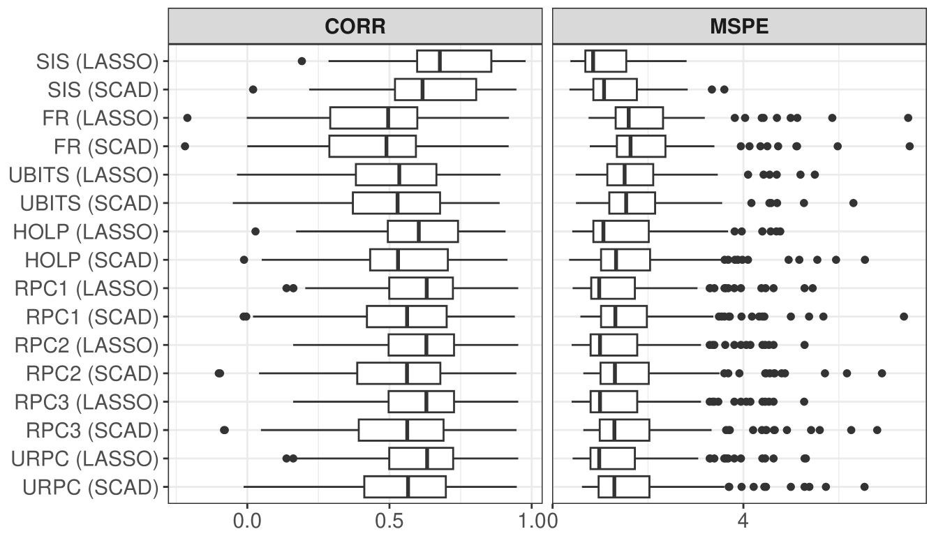
	SCAD		LASSO
	Mean	SE	Mean	SE
SIS	7.91	3.54	16.60	2.22
FR	50.66	1.66	62.34	4.70
UBITS	32.42	13.60	37.33	15.55
HOLP	23.33	4.73	38.23	5.24
RPC1	26.65	3.48	43.45	5.93
RPC2	26.80	3.70	43.39	5.76
RPC3	26.46	3.88	43.41	5.86
URPC	26.75	4.17	43.73	6.10

Figure 1: Prediction accuracy on the test sets: correlation (top left), MSPE ($\times 10^{-4}$, top right). The mean model sizes and their standard errors are shown in the table.

6 Discussion

In this paper, we develop a ridge partial correlation (RPC) method for screening variables in an ultrahigh-dimensional regression model. RPC screening does not require strong assumptions on marginal correlations, which means that it can be applied to more data sets with complex correlation structures than the SIS. Theoretically, as $n,p\to\infty$, the RPC screening will produce the same model as the HOLP, which ensures that the performance of the RPC screening is not worse than the HOLP. We show that the RPC screening leads to better performance in the extreme correlation cases where the marginal correlations between the response and unimportant variables are larger than the same between the response and the true predictors. Finally, we show that the RPC screening can be fast implemented by using Cholesky decomposition and parallel computing.

The definition of ridge partial correlation does not require the linear regression assumption. RPC screening can also be extended to larger classes of regression models, for example the generalized linear regression models. Potential future works include developing RPC screening methods for generalized additive models.

Supplement to
“Ridge partial correlation screening for ultrahigh-dimensional data”
Run Wang, An Nguyen, Somak Dutta, and Vivekananda Roy

S1 Some notations

The following notations will be used in the proof of Theorem 1:

• $\mathcal{O}(n)$ denotes the $n$th order orthogonal group.

• The Stiefel manifold $V_{n,p}$ is the set of $p\times n$ matrices $A$ such that $A^{\top}A=I_{n}$ [Chikuse, 2003].

For any $\lambda>0$,

• $\hat{\beta}(\lambda)=(X^{\top}X+\lambda I)^{-1}X^{\top}\tilde{Y}=X^{\top}(XX^{\top}+\lambda I)^{-1}\tilde{Y}$ is the ridge regression estimator of $\beta$.

• $Z=VDU^{\top}$ is the singular value decomposition of $Z$, where $V\in\mathcal{O}(n)$, $U\in V_{n,p}$, and $D$ is an $n\times n$ diagonal matrix. Thus, $X=VDU^{\top}\Sigma^{1/2}$.

• $A=(U^{\top}\Sigma U)^{1/2}$ satisfies $A^{\top}A=AA^{\top}=A^{2}$.

• $H=\Sigma^{1/2}U(U^{\top}\Sigma U)^{-1/2}$ satisfies $H^{\top}H=I_{n}$.

• $M=\sum_{k=1}^{\infty}\lambda^{k}\Sigma^{1/2}UA^{-1}(A^{-\top}D^{-2}A^{-1})^{k}A^{-\top}U^{\top}\Sigma^{1/2}$.

• $\xi_{i}$ is the $i$th diagonal element of $(X^{\top}X+\lambda I)^{-1},i=1,\dots,p$.

S2 Some useful lemmas

In this Section, we present some useful lemmas which will be used in the proof of Theorem 1.

Lemma 1.

In Definition 1, $v_{iy,\lambda}$ is the same as the $i$th element of

$$\dfrac{-(X^{\top}X+\lambda I)^{-1}X^{\top}\tilde{Y}}{S_{\lambda}},$$

$v_{i,\lambda}$ is the same as $i$th diagonal element of

$$(X^{\top}X+\lambda I)^{-1}+\dfrac{(X^{\top}X+\lambda I)^{-1}X^{\top}\tilde{Y}\tilde{Y}^{\top}X(X^{\top}X+\lambda I)^{-1}}{S_{\lambda}},$$

and

$$v_{y,\lambda}=\dfrac{1}{S_{\lambda}}.$$

Proof.

By block matrix inverse formula,

$$\bm{R} =n\begin{pmatrix}\tilde{Y}^{\top}\tilde{Y}&\tilde{Y}^{\top}X\\ X^{\top}\tilde{Y}&X^{\top}X+\lambda I\end{pmatrix}^{-1}$$

$$=n\begin{pmatrix}\bm{A_{\lambda}}&\bm{B_{\lambda}}\\ \bm{C_{\lambda}}&\bm{D_{\lambda}}\end{pmatrix}$$

where

$$\begin{split}&\bm{A_{\lambda}}=\dfrac{1}{S_{\lambda}},\\ &\bm{B_{\lambda}}=-\dfrac{\tilde{Y}^{\top}X(X^{\top}X+\lambda I)^{-1}}{S_{\lambda}},\\ &\bm{C_{\lambda}}=-\dfrac{(X^{\top}X+\lambda I)^{-1}X^{\top}\tilde{Y}}{S_{\lambda}},\;\mbox{and}\\ &\bm{D_{\lambda}}=(X^{\top}X+\lambda I)^{-1}+\dfrac{(X^{\top}X+\lambda I)^{-1}X^{\top}\tilde{Y}\tilde{Y}^{\top}X(X^{\top}X+\lambda I)^{-1}}{S_{\lambda}}.\end{split}$$

Then the proof follows from Definition 1 and an application of the standard block matrix inversion formula. ∎

The following lemma is a well known result in linear algebra.

Lemma 2.

For any $n\times n$ positive semidefinite matrices $A$ and $B$, we have $\alpha_{max}(A+B)\leq\alpha_{max}(A)+\alpha_{max}(B),\alpha_{max}(AB)\leq\alpha_{max}(A)\alpha_{max}(B),\alpha_{min}(AB)\geq\alpha_{min}(A)\alpha_{min}(B).$

Proof.

A proof can be found in Horn and Johnson [1985]. ∎

The following lemma is the Lemma 4 in Wang and Leng [2016].

Lemma 3 (Wang and Leng [2016]).

Under assumptions A1 - A3, for any $C>0$ and any fixed vector $v$ with $\|v\|=1$, there exist $c_{1}^{\prime},c_{2}^{\prime}$ only related to $C$ with $0<c_{1}^{\prime}<1<c_{2}^{\prime}$ such that

$$P\left(v^{\top}HH^{\top}v<c_{1}^{\prime}\dfrac{n^{1-\tau}}{p}\quad\text{or}\quad v^{\top}HH^{\top}v>c_{2}^{\prime}\dfrac{n^{1+\tau}}{p}\right)<4e^{-Cn},$$

for $H$ defined in Section S1. In particular, for $v=\beta$, a similar inequality holds for one side with a new $c_{2}^{\prime}$ as

$$P\left(\beta^{\top}HH^{\top}\beta>c_{2}^{\prime}\dfrac{n^{1+\tau}}{p}\right)<2e^{-Cn}.$$

S3 Proof of Theorem 1

We first provide a sketch of the proof. By (5) in Definition 1 and Lemma 1, the ridge partial correlation can be rewritten as

$$R_{i,\lambda}=-\dfrac{\hat{\beta}_{i}(\lambda)}{\left\{S_{\lambda}\xi_{i}+\hat{\beta}_{i}(\lambda)^{2}\right\}^{1/2}},$$ (S1)

where $\hat{\beta}_{i}(\lambda)$ is the $i$th element of the ridge regression estimator $\hat{\beta}(\lambda)$ and $\xi_{i}$ is the $i$th diagonal element of $(X^{\top}X+\lambda I)^{-1}$ as defined in Section S1. Thus, it follows that

$$\dfrac{S_{\lambda}R_{i,\lambda}^{2}}{1-R_{i,\lambda}^{2}}=\dfrac{\hat{\beta}_{i}^{2}(\lambda)}{\xi_{i}}.$$

By Theorem 3 in Wang and Leng [2016], we have a separation on $|\hat{\beta}_{i}(\lambda)|$ for $i\in t$ and $i\notin t$. Therefore if we can show that $\lambda\xi_{i}\stackrel{{\scriptstyle p}}{{\to}}1$ uniformly, then we will have a separation on $S_{\lambda}R_{i,\lambda}^{2}/(1-R_{i,\lambda}^{2})$ as stated in Theorem 1. Next, we provide a proof of Theorem 1.

Proof.

From Section S1, since $X=VDU^{\top}\Sigma^{1/2}$, we have

$$\begin{split}X^{\top}(XX^{\top}+\lambda I)^{-1}X&=\Sigma^{1/2}UDV^{\top}(VDU^{\top}\Sigma UDV^{\top}+\lambda I)^{-1}VDU^{\top}\Sigma^{1/2}\\ &=\Sigma^{1/2}U(U^{\top}\Sigma U+\lambda D^{-2})^{-1}U^{\top}\Sigma^{1/2}\\ &=\Sigma^{1/2}UA^{-1}(I+\lambda A^{-\top}D^{-2}A^{-1})^{-1}A^{-\top}U^{\top}\Sigma^{1/2}.\end{split}$$ (S2)

In order to use Taylor expansion on the inverse matrix in (S2), we need to consider the maximum eigenvalue of $A^{-\top}D^{-2}A^{-1}$. By Lemma 2,

$$\alpha_{\max}(A^{-\top}D^{-2}A^{-1})\leq\alpha_{\max}(D^{-2})\alpha_{\max}((AA^{\top})^{-1})=\alpha_{\min}(D^{2})^{-1}\alpha_{\min}(U^{\top}\Sigma U)^{-1}.$$

From the assumption A2, we have

$$P(p^{-1}\alpha_{\min}(D^{2})<c_{1}^{-1})<e^{-C_{1}n}$$

for some $c_{1}>1$ and $C_{1}>0$. Also, by Lemma 2 and the assumption A3, we have

$$\alpha_{\min}(U^{\top}\Sigma U)\geq\alpha_{\min}(\Sigma)\alpha_{\min}(U^{\top}U)\geq c_{4}^{-1}n^{-\tau}.$$

Therefore, with probability greater than $1-e^{-C_{1}n}$, we have

$$\alpha_{\max}(\lambda A^{-\top}D^{-2}A^{-1})\leq\dfrac{c_{1}c_{4}\lambda n^{\tau}}{p}<1$$ (S3)

since by the assumption A4, $p\succ n^{1+\tau}$ and $\lambda\prec n^{1-(5/2)\tau-\kappa}$.

Thus, the Taylor expansion gives that

$$\begin{split}&\Sigma^{1/2}UA^{-1}(I+\lambda A^{-\top}D^{-2}A^{-1})^{-1}A^{-\top}U^{\top}\Sigma^{1/2}\\ &=\Sigma^{1/2}UA^{-1}\Bigg{(}I+\sum_{k=1}^{\infty}\lambda^{k}(A^{-\top}D^{-2}A^{-1})^{k}\Bigg{)}A^{-\top}U^{\top}\Sigma^{1/2}\\ &=HH^{\top}+M,\end{split}$$ (S4)

where $H$ and $M$ are as defined in Appendix S1.

By Lemma 2, we have

$$\begin{split}&\alpha_{\max}(\Sigma^{1/2}UA^{-1}(A^{-\top}D^{-2}A^{-1})^{k}A^{-\top}U^{\top}\Sigma^{1/2})\\ &\leq\alpha_{\max}(\Sigma^{1/2}UA^{-1}A^{-\top}U^{\top}\Sigma^{1/2})\alpha_{\max}(A^{-\top}D^{-2}A^{-1})^{k}\\ &=\alpha_{\max}(HH^{\top})\alpha_{\max}(A^{-\top}D^{-2}A^{-1})^{k}\\ &\leq\alpha_{\max}(A^{-\top}D^{-2}A^{-1})^{k}.\end{split}$$ (S5)

Combining (S3), (S5) and Lemma 2, we have an upper bound for the largest eigenvalue of $M$ given by

$$\alpha_{\max}(M)\leq\sum_{k=1}^{\infty}\lambda^{k}\alpha_{\max}(A^{-\top}D^{-2}A^{-1})^{k}\leq\dfrac{\lambda\alpha_{\max}(A^{-\top}D^{-2}A^{-1})}{1-\lambda\alpha_{\max}(A^{-\top}D^{-2}A^{-1})}.$$ (S6)

Since $g/(1-g)$ is an increasing function of $g$, from (S3), (S6) and the assumption A4, we have

$$\begin{split}P\left(\alpha_{\max}(M)>\dfrac{c_{1}c_{4}\lambda n^{\tau}}{p-c_{1}c_{4}\lambda n^{\tau}}\right)&<P\left(\dfrac{\lambda\alpha_{\max}(A^{-\top}D^{-2}A^{-1})}{1-\lambda\alpha_{\max}(A^{-\top}D^{-2}A^{-1})}>\dfrac{c_{1}c_{4}\lambda n^{\tau}}{p-c_{1}c_{4}\lambda n^{\tau}}\right)\\ &=P\left(\alpha_{\max}(A^{-\top}D^{-2}A^{-1})>\dfrac{c_{1}c_{4}n^{\tau}}{p}\right)<e^{-C_{1}n}.\end{split}$$ (S7)

By the Woodbury identity, (S2), and (S4), we have

$$(X^{\top}X+\lambda I)^{-1}=\dfrac{1}{\lambda}I-\dfrac{1}{\lambda}X^{\top}(XX^{\top}+\lambda I)^{-1}X=\dfrac{1}{\lambda}I-\dfrac{1}{\lambda}(HH^{\top}+M),$$ (S8)

and hence

$$\xi_{i}=\dfrac{1}{\lambda}-\dfrac{1}{\lambda}e_{i}^{\top}HH^{\top}e_{i}-\dfrac{1}{\lambda}e_{i}^{\top}Me_{i},$$ (S9)

where $e_{i}=(0,\dots,0,1,0,\dots,0)^{\top}$ is the $i$th vector in the standard basis for $\mathcal{R}^{p}$. By Lemma 3, we have

$$P\left(e_{i}^{\top}HH^{\top}e_{i}<c_{2}^{\prime}\dfrac{n^{1+\tau}}{p}\right)>1-4e^{-Cn}$$ (S10)

uniformly for all $i$. Also, by (S7), we have

$$P\left(e_{i}^{\top}Me_{i}>\dfrac{c_{1}c_{4}\lambda n^{\tau}}{p-c_{1}c_{4}\lambda n^{\tau}}\right)\leq P\left(\alpha_{\max}(M)>\dfrac{c_{1}c_{4}\lambda n^{\tau}}{p-c_{1}c_{4}\lambda n^{\tau}}\right)<e^{-C_{1}n}$$ (S11)

uniformly for all $i$.

Combining (S10) and (S11) and using Bonferroni’s inequality, we have

$$P\left(\max_{i}(e_{i}^{\top}HH^{\top}e_{i}+e_{i}^{\top}Me_{i})>c_{2}^{\prime}\dfrac{n^{1+\tau}}{p}+\dfrac{c_{1}c_{4}\lambda n^{\tau}}{p-c_{1}c_{4}\lambda n^{\tau}}\right)\leq p(4e^{-Cn}+e^{-C_{1}n})\to 0$$ (S12)

as $n\to\infty$. From (S9), we have $\xi_{i}<1/\lambda$. Thus, by (S9) and (S12), we have

$$P\left(\max_{i}(|\lambda\xi_{i}-1|)>c_{2}^{\prime}\dfrac{n^{1+\tau}}{p}+\dfrac{c_{1}c_{4}\lambda n^{\tau}}{p-c_{1}c_{4}\lambda n^{\tau}}\right)\leq p(4e^{-Cn}+e^{-C_{1}n}).$$ (S13)

By the assumption A4,

$$\dfrac{n^{1+\tau}}{p}\to 0,\quad\text{and}\quad\dfrac{c_{1}c_{4}\lambda n^{\tau}}{p-c_{1}c_{4}\lambda n^{\tau}}\to 0$$

as $n\to\infty$, which means that $\lambda\xi_{i}\stackrel{{\scriptstyle p}}{{\to}}1$ uniformly.

We denote $c_{2}^{\prime}n^{1+\tau}/p+c_{1}c_{4}\lambda n^{\tau}/(p-c_{1}c_{4}\lambda n^{\tau})$ by $\eta_{n}$ which is an infinitesimal. Let $\{\rho_{n}\}_{n\geq 1}$ be a sequence satisfying

$$\dfrac{1}{\sqrt{1-\eta_{n}}}\left(\dfrac{\tilde{c}+\sigma\sqrt{2C_{1}c_{1}c_{2}^{\prime}c_{4}}}{\sqrt{\log n}}+\dfrac{c_{1}c_{4}\sqrt{c^{\prime}c_{4}}\lambda n^{5/2\tau+\kappa-1}}{1-c_{1}c_{4}\lambda n^{\tau}/p}\right)\dfrac{n^{1-\tau-\kappa}}{p}<\sqrt{\dfrac{\rho_{n}^{2}}{\lambda}}<\dfrac{c}{4}\dfrac{n^{1-\tau-\kappa}}{p},$$ (S14)

where $c$ and $\tilde{c}$ are constants as in the proof of Theorem 3 in Wang and Leng [2016]. Since

$$\lim\limits_{n\to 0}\dfrac{1}{\sqrt{1-\eta_{n}}}\left(\dfrac{\tilde{c}+\sigma\sqrt{2C_{1}c_{1}c_{2}^{\prime}c_{4}}}{\sqrt{\log n}}+\dfrac{c_{1}c_{4}\sqrt{c^{\prime}c_{4}}\lambda n^{5/2\tau+\kappa-1}}{1-c_{1}c_{4}\lambda n^{\tau}/p}\right)=0,$$

the $\rho_{n}$ in (S14) always exists.

Note that $1/R^{2}_{i,\lambda}=1+\xi_{i}\times S_{\lambda}/\hat{\beta}_{i}(\lambda)^{2}$. By the proof of Theorem 3 in Wang and Leng [2016] (see Supplementary of Wang and Leng [2016]), (S13), and the assumption A4, we have

$$\begin{split}P\left(\max_{i\notin t}\dfrac{S_{\lambda}R_{i,\lambda}^{2}}{1-R_{i,\lambda}^{2}}>\rho^{2}_{n}\right)&=P\left(\max_{i\notin t}\dfrac{\hat{\beta}_{i}^{2}(\lambda)}{\xi_{i}}>\rho_{n}^{2}\right)\\ &\leq P\left(\dfrac{\max_{i\notin t}\hat{\beta}_{i}^{2}(\lambda)}{\min_{i\notin t}\xi_{i}}>\rho_{n}^{2}\right)\\ &=P\left(\max_{i\notin t}\hat{\beta}^{2}_{i}(\lambda)>\rho_{n}^{2}\min_{i\notin t}\xi_{i}\right)\\ &\leq P\left(\max_{i\notin t}\hat{\beta}^{2}_{i}(\lambda)>\dfrac{\rho^{2}(1-\eta_{n})}{\lambda},\min_{i\notin t}\lambda\xi_{i}>1-\eta_{n}\right)+P\left(\min_{i\notin t}\lambda\xi_{i}<1-\eta_{n}\right)\\ &\leq P\left(\max_{i\notin t}\hat{\beta}^{2}_{i}(\lambda)>(1-\eta_{n})\dfrac{\rho^{2}_{n}}{\lambda}\right)+P\left(\max_{i\notin t}(1-\lambda\xi_{i})>\eta_{n}\right)\\ &\leq P\left(\max_{i\notin t}\hat{\beta}^{2}_{i}(\lambda)>\left[\left(\dfrac{\tilde{c}+\sigma\sqrt{2C_{1}c_{1}c_{2}^{\prime}c_{4}}}{\sqrt{\log n}}+\dfrac{c_{1}c_{4}\sqrt{c^{\prime}c_{4}}\lambda n^{5/2\tau+\kappa-1}}{1-c_{1}c_{4}\lambda n^{\tau}/p}\right)\dfrac{n^{1-\tau-\kappa}}{p}\right]^{2}\right)\\ &+P\left(\max_{i\notin t}(1-\lambda\xi_{i})>\eta_{n}\right)\\ &\leq O\bigg{(}\exp\bigg{\{}-C_{1}\dfrac{n^{1-5\tau-2\kappa-\nu}}{2\log(n)}\bigg{\}}\\ &+\exp\bigg{[}1-\dfrac{1}{2}q\bigg{(}\dfrac{\sqrt{C_{1}}n^{1/2-2\tau-\kappa}}{\sqrt{\log(n)}}\bigg{)}\bigg{]}\bigg{)}+p(4e^{-Cn}+e^{-C_{1}n}).\end{split}$$ (S15)

Similarly, since $\xi_{i}<1/\lambda$, we have

$$\begin{split}P\left(\min_{i\in t}\dfrac{S_{\lambda}R_{i,\lambda}^{2}}{1-R_{i,\lambda}^{2}}<\rho^{2}_{n}\right)&=P\left(\min_{i\in t}\dfrac{\hat{\beta}_{i}^{2}(\lambda)}{\xi_{i}}<\rho_{n}^{2}\right)\\ &=P\left(\dfrac{\min_{i\in t}\hat{\beta}_{i}^{2}(\lambda)}{\max_{i\in t}\xi_{i}}<\rho_{n}^{2}\right)\\ &\leq P\left(\min_{i\in t}\hat{\beta}^{2}_{i}(\lambda)<\dfrac{\rho^{2}_{n}}{\lambda}\right)\\ &<P\left(\min_{i\in t}\hat{\beta}^{2}_{i}(\lambda)<\left[\dfrac{c}{4}\dfrac{n^{1-\tau-\kappa}}{p}\right]^{2}\right)\\ &<O\bigg{(}\exp\bigg{\{}-C_{1}\dfrac{n^{1-5\tau-2\kappa-\nu}}{2\log(n)}\bigg{\}}+\exp\bigg{[}1-\dfrac{1}{2}q\bigg{(}\dfrac{\sqrt{C_{1}}n^{1/2-2\tau-\kappa}}{\sqrt{\log(n)}}\bigg{)}\bigg{]}\bigg{)},\end{split}$$ (S16)

where the last inequality follows from the proof of Theorem 3 in Wang and Leng [2016].

By the assumption A4, $\log(p)\prec n^{1-2\kappa-5\tau}/[2\log(n)]$ and hence,

$$p(4e^{-Cn}+e^{-C_{1}n})\prec\exp\bigg{\{}-C_{1}\dfrac{n^{1-5\tau-2\kappa-\nu}}{2\log(n)}\bigg{\}}.$$

This result combined with (S15) and (S16) gives

$$\begin{split}P\bigg{(}\min_{i\in t}\dfrac{S_{\lambda}R_{i,\lambda}^{2}}{1-R_{i,\lambda}^{2}}&>\rho^{2}_{n}>\max_{i\notin t}\dfrac{S_{\lambda}R_{i,\lambda}^{2}}{1-R_{i,\lambda}^{2}}\bigg{)}\\ &=1-O\bigg{(}\exp\bigg{\{}-C_{1}\dfrac{n^{1-5\tau-2\kappa-\nu}}{2\log(n)}\bigg{\}}+\exp\bigg{[}1-\dfrac{1}{2}q\bigg{(}\dfrac{\sqrt{C_{1}}n^{1/2-2\tau-\kappa}}{\sqrt{\log(n)}}\bigg{)}\bigg{]}\bigg{)}.\end{split}$$

Since $g/(1-g)$ is an increasing function of $g$, if we choose a submodel with size $K_{n}\geq|t|$, we will have

$$P(t\subset\gamma^{K_{n}})=1-O\left[\exp\left\{-C_{1}\dfrac{n^{1-2\kappa-5\tau-\nu}}{2\log(n)}\right\}+\exp\left\{1-\dfrac{1}{2}q\left(\dfrac{\sqrt{C_{1}}n^{1/2-2\tau-\kappa}}{\sqrt{\log(n)}}\right)\right\}\right]$$

which completes the whole proof. ∎

S4 Additional simulation results

In this section, we present results from simulation settings corresponding to different $R^{2}$ values and error distributions. The results are reported as percentages.

Table S1: Additional simulation results for normally distributed errors

Method	Correlation Structure
	Theoretical $R^{2}=0.1$
	IID		Compound		Group		AR		Factor		ExtrCor		SpFactor
	TPR	CP	TPR	CP	TPR	CP	TPR	CP	TPR	CP	TPR	CP	TPR	CP
RPC1	43.4	0	9.9	0	82.2	46	75.4	18	12.1	0	66.2	3	38.8	0
RPC2	43.6	0	9.9	0	82.3	46	75.6	18	12.1	0	66.4	3	38.9	0
RPC3	43.4	0	9.9	0	82.2	46	75.3	18	12.1	0	66.6	3	38.7	0
URPC	43.6	0	9.9	0	82.3	46	75.6	18	12.2	0	67.0	3	38.9	0
UBITS	45.6	0	17.3	0	87.8	64	69.4	5	20.1	0	16.3	0	55.3	1
HOLP	43.4	0	9.9	0	82.4	47	75.3	18	12.1	0	59.2	1	39.1	0
FR	15.4	0	6.2	0	21.0	0	21.0	0	7.9	0	9.1	0	9.3	0
SIS	46.2	0	14.2	0	88.4	63	83.2	29	20.0	0	1.9	0	48.3	0
	Theoretical $R^{2}=0.3$
	IID		Compound		Group		AR		Factor		ExtrCor		SparseFactor
	TPR	CP	TPR	CP	TPR	CP	TPR	CP	TPR	CP	TPR	CP	TPR	CP
RPC1	89	33	24	0	100	100	100	98	18	0	92	46	63	2
RPC2	89	33	24	0	100	100	100	98	18	0	92	45	64	2
RPC3	89	33	24	0	100	100	100	98	18	0	92	46	63	2
URPC	89	33	24	0	100	100	100	98	18	0	92	47	64	2
UBITS	90	35	29	0	100	100	98	85	29	0	62	6	74	6
HOLP	89	33	24	0	100	100	100	98	18	0	90	37	64	2
FR	57	0	10	0	37	0	42	0	8	0	19	0	16	0
SIS	90	39	35	0	100	100	100	99	21	0	0	0	68	2
	Theoretical $R^{2}=0.4$
	IID		Compound		Group		AR		Factor		ExtrCor		SpFactor
	TPR	CP	TPR	CP	TPR	CP	TPR	CP	TPR	CP	TPR	CP	TPR	CP
RPC1	96	69	32.4	0	100	100	99.9	99	36	0	97.4	80	69.0	1
RPC2	96	69	32.4	0	100	100	99.9	99	36.2	0	97.6	81	69.0	1
RPC3	96	69	32.3	0	100	100	99.9	99	36	0	97.3	79	69.0	1
URPC	96	69	32.6	0	100	100	99.9	99	36.2	0	97.6	81	69.0	1
UBITS	96.8	75	35.7	0	100	100	99.6	96	45.3	2	89.8	57	78.7	7
HOLP	96	69	32.4	0	100	100	99.9	99	36.4	0	95.6	67	69.1	1
FR	82.8	30	11.7	0	36.8	0	50.6	0	13.6	0	38.6	4	17.4	0
SIS	96.4	71	41.7	0	100.0	100	100.0	100	20.2	0	0.0	0	72.8	3

Table S2: Simulation results for $t$ distributed errors

Method	Correlation Structure
	Theoretical $R^{2}=0.1$
	IID		Compound		Group		AR		Factor		ExtrmCor		SparseFactor
	TPR	CP	TPR	CP	TPR	CP	TPR	CP	TPR	CP	TPR	CP	TPR	CP
RPC1	43.6	0	10.6	0	80.6	40	78.7	19	10.7	0	67.1	2	41.1	0
RPC2	43.6	0	10.6	0	80.6	40	78.7	19	10.7	0	67.2	2	41.1	0
RPC3	43.6	0	10.4	0	80.4	40	78.6	19	10.7	0	67.0	2	41.1	0
URPC	43.6	0	10.6	0	80.6	40	78.7	19	10.8	0	67.3	2	41.1	0
UBITS	46.1	0	17.8	0	87.3	62	71.9	7	17.8	0	16.8	0	57.2	2
HOLP	43.6	0	10.6	0	80.9	42	78.6	19	10.9	0	59.4	0	41.2	0
FR	16.2	0	6.3	0	21.9	0	22.7	0	7.1	0	8.9	0	9.0	0
SIS	45.6	0	16.1	0	87.7	68	82.6	26	19.0	0	4.2	0	50.3	1
	Theoretical $R^{2}=0.2$
	IID		Compound		Group		AR		Factor		ExtrmCor		SparseFactor
	TPR	CP	TPR	CP	TPR	CP	TPR	CP	TPR	CP	TPR	CP	TPR	CP
RPC1	74.3	6	17.7	0	99.1	96	96.1	70	14.2	0	82.3	20	54.4	0
RPC2	74.3	6	17.7	0	99.1	96	96.1	70	14.7	0	82.4	20	54.5	0
RPC3	74.3	6	17.7	0	99.1	96	96.1	70	14.1	0	82.3	20	54.4	0
URPC	74.3	6	17.7	0	99.1	96	96.1	70	14.8	0	82.6	20	54.5	0
UBITS	75.1	6	24.3	0	99.9	99	92.3	45	22.3	0	41.8	1	68.8	1
HOLP	74.3	6	17.7	0	99.1	96	96.1	70	14.4	0	78.2	8	54.5	0
FR	34.7	0	8.0	0	34.1	0	33.1	0	7.9	0	12.8	0	13.0	0
SIS	76.3	8	24.9	0	99.6	97	98.2	84	20.9	0	0.3	0	61.4	0
	Theoretical $R^{2}=0.3$
	IID		Compound		Group		AR		Factor		ExtrmCor		SparseFactor
	TPR	CP	TPR	CP	TPR	CP	TPR	CP	TPR	CP	TPR	CP	TPR	CP
RPC1	88.8	30	22.7	0	100.0	100	98.8	89	23.7	0	91.2	44	63.2	1
RPC2	88.8	30	22.7	0	100.0	100	98.8	89	23.8	0	91.1	45	63.2	1
RPC3	88.8	30	22.7	0	100.0	100	98.8	89	23.7	0	91.3	45	63.2	1
URPC	88.8	30	22.7	0	100.0	100	98.8	89	23.8	0	91.6	47	63.2	1
UBITS	89.2	35	28.4	0	100.0	100	98.1	85	31.6	0	62.6	5	74.8	5
HOLP	88.8	30	22.7	0	100.0	100	98.8	89	24.0	0	88.8	35	63.2	1
FR	57.3	3	7.6	0	36.3	0	42.9	0	10.3	0	17.9	0	15.8	0
SIS	89.2	33	30.8	0	100.0	100	98.9	90	18.8	0	0.0	0	68.4	3
	Theoretical $R^{2}=0.4$
	IID		Compound		Group		AR		Factor		ExtrmCor		SparseFactor
	TPR	CP	TPR	CP	TPR	CP	TPR	CP	TPR	CP	TPR	CP	TPR	CP
RPC1	95.6	65	35.2	0	100.0	100	100.0	100	29.3	0	96.8	74	62.9	2
RPC2	95.6	65	35.3	0	100.0	100	100.0	100	29.1	0	96.8	74	63.0	2
RPC3	95.6	65	35.2	0	100.0	100	100.0	100	28.9	0	96.9	75	62.9	2
URPC	95.6	65	35.4	0	100.0	100	100.0	100	29.4	0	96.9	75	63.0	2
UBITS	95.6	68	38.9	0	100.0	100	99.8	98	37.8	1	88.2	52	74.1	5
HOLP	95.6	65	35.1	0	100.0	100	100.0	100	29.7	0	94.7	61	63.2	2
FR	83.1	33	12.7	0	37.4	0	51.1	0	12.9	0	37.0	4	16.4	0
SIS	95.6	65	41.1	0	100.0	100	100.0	100	22.1	0	0.0	0	66.1	4

Table S3: Simulation results for exponentially distributed errors

Method	Correlation Structure
	Theoretical $R^{2}=0.1$
	IID		Compound		Group		AR		Factor		ExtrmCor		SparseFactor
	TPR	CP	TPR	CP	TPR	CP	TPR	CP	TPR	CP	TPR	CP	TPR	CP
RPC1	45.6	0	10.7	0	82.3	44	77.2	18	9.3	0	67.1	2	41.4	0
RPC2	45.6	0	10.7	0	82.3	44	77.2	18	9.3	0	67.2	2	41.4	0
RPC3	45.6	0	10.7	0	82.2	44	77.2	18	9.3	0	66.9	2	41.3	0
URPC	45.6	0	10.7	0	82.3	44	77.2	18	9.4	0	67.4	2	41.4	0
UBITS	48.3	1	18.0	0	86.7	66	73.3	12	17.2	0	18.8	0	58.1	1
HOLP	45.7	0	10.7	0	82.3	44	77.2	18	9.4	0	61.0	0	41.6	0
FR	15.1	0	6.3	0	22.4	0	23.0	0	6.9	0	8.7	0	8.9	0
SIS	47.0	0	17.4	0	88.8	60	82.8	25	17.6	0	1.3	0	51.0	0

References

- Bai et al. [2022] Ray Bai, Gemma E. Moran, Joseph Antonelli, Yong Chen, and Mary Regina Boland. Spike-and-slab group lassos for grouped regression and sparse generalized additive models. Journal of the American Statistical Association, 117(537):184–197, 2022.
- Chikuse [2003] Yasuko Chikuse. Statistics on special manifolds. Springer New York, 2003. doi: 10.1007/978-0-387-21540-2.
- Cho and Fryzlewicz [2012] Haeran Cho and Piotr Fryzlewicz. High dimensional variable selection via tilting. Journal of the Royal Statistical Society, Series B, 74(3):593–622, 2012.
- Dutta and Nguyen [2025] Somak Dutta and An Nguyen. rpc: Ridge Partial Correlation, 2025. URL https://CRAN.R-project.org/package=rpc. R package version 2.0.3.
- Fan and Li [2001] J. Fan and R. Li. Variable selection via nonconcave penalized likelihood and its oracle property. Journal of the American Statistical Association, 96:1348–1360, 2001.
- Fan and Lv [2008] Jianqing Fan and Jinchi Lv. Sure independence screening for ultrahigh dimensional feature space. Journal of Royal Statistical Society, Series B, 70(5):849–911, 2008.
- Fan and Song [2010] Jianqing Fan and Rui Song. Sure independence screening in generalized linear models with NP-dimensionality. The Annals of Statistics, 38(6):3567–3604, 2010.
- Fan et al. [2011] Jianqing Fan, Yang Feng, and Rui Song. Nonparametric independence screening in sparse ultra-high-dimensional additive models. Journal of the American Statistical Association, 106(494):544–557, 2011.
- Gorst-Rasmussen and Scheike [2013] Anders Gorst-Rasmussen and Thomas Scheike. Independent screening for single-index hazard rate models with ultrahigh dimensional features. Journal of the Royal Statistical Society Series B: Statistical Methodology, 75(2):217–245, 2013.
- Hall and Miller [2009] Peter Hall and Hugh Miller. Using generalized correlation to effect variable selection in very high dimensional problems. Journal of Computational and Graphical Statistics, 18(3):533–550, 2009.
- Hao and Zhang [2014] Ning Hao and Hao Helen Zhang. Interaction screening for ultrahigh-dimensional data. Journal of the American Statistical Association, 109(507):1285–1301, 2014.
- Hoerl and Kennard [1970] A. E. Hoerl and R. W. Kennard. Ridge regression: Biased estimation for nonorthogonal problems. Technometrics, 12:55–67, 1970.
- Horn and Johnson [1985] Roger A. Horn and Charles R. Johnson. Matrix Analysis. Cambridge University Press, 1985. doi: 10.1017/CBO9780511810817.
- Huang et al. [2008] Jian Huang, Joel L Horowitz, and Shuangge Ma. Asymptotic properties of bridge estimators in sparse high-dimensional regression models. The Annals of Statistics, 36(2):587–613, 2008.
- Li et al. [2012a] Gaorong Li, Heng Peng, Jun Zhang, and Lixing Zhu. Robust rank correlation based screening. The Annals of Statistics, 40(3):1846–1877, 2012a.
- Li et al. [2012b] Runze Li, Wei Zhong, and Liping Zhu. Feature screening via distance correlation learning. Journal of the American Statistical Association, 107(499):1129–1139, 2012b.
- Lin and Pang [2014] Bingqing Lin and Zhen Pang. Tilted correlation screening learning in high-dimensional data analysis. Journal of Computational and Graphical Statistics, 23(2):478–496, 2014.
- Ma et al. [2017] Shujie Ma, Runze Li, and Chih-Ling Tsai. Variable screening via quantile partial correlation. Journal of the American Statistical Association, 112(518):650–663, 2017.
- Scheetz et al. [2006] Todd E. Scheetz, Kwang-Youn A. Kim, Ruth E. Swiderski, Alisdair R. Philp, Terry A. Braun, Kevin L. Knudtson, Anne M. Dorrance, Gerald F. DiBona, Jian Huang, Thomas L. Casavant, Val C. Sheffield, and Edwin M. Stone. Regulation of gene expression in the mammalian eye and its relevance to eye disease. Proceedings of the National Academy of Sciences, 103(39):14429–14434, 2006. ISSN 0027-8424. doi: 10.1073/pnas.0602562103. URL https://www.pnas.org/content/103/39/14429.
- Tibshirani [1996] R. Tibshirani. Regression shrinkage and selection via the lasso. Journal of the Royal Statistical Society, Series B, 58:267–288, 1996.
- Vershynin [2012] Roman Vershynin. Introduction to the non-asymptotic analysis of random matrices. In Yonina C. Eldar and GittaEditors Kutyniok, editors, Compressed Sensing: Theory and Applications, page 210–268. Cambridge University Press, 2012. doi: 10.1017/CBO9780511794308.006.
- Wang [2009] Hansheng Wang. Forward regression for ultra-high dimensional variable screening. Journal of the American Statistical Association, 104(488):1512–1524, 2009.
- Wang et al. [2021] Run Wang, Somak Dutta, and Vivekananda Roy. A note on marginal correlation based screening. Statistical Analysis and Data Mining: The ASA Data Science Journal, 14(1):88–92, 2021.
- Wang et al. [2025] Run Wang, Somak Dutta, and Vivekananda Roy. Bayesian iterative screening in ultra-high dimensional linear regressions. Bayesian Analysis, 2025. Advance Publication 1-26, https://doi.org/10.1214/25-BA1517.
- Wang and Leng [2016] Xiangyu Wang and Chenlei Leng. High dimensional ordinary least squares projection for screening variables. Journal of the Royal Statistical Society: Series B (Statistical Methodology), 78(3):589–611, 2016.
- Zhao and Li [2012] Sihai Dave Zhao and Yi Li. Principled sure independence screening for cox models with ultra-high-dimensional covariates. Journal of multivariate analysis, 105(1):397–411, 2012.
- Zou [2006] H. Zou. The adaptive lasso and its oracle properties. Journal of the American Statistical Association, 101:1418–1429, 2006.
- Zou and Hastie [2005] H. Zou and T. Hastie. Regularization and variable selection via the Elastic Net. Journal of the Royal Statistical Society, Series B, 67:301–320, 2005.