Electron Wave-Spin Qubit

Abstract

This work proposes a wave-entity perspective of the electron spin qubit, treating the electron as a continuous physical wave rather than a point-like particle. In this theoretical framework, each spin qubit corresponds to a distinct current density configuration, offering a resolution to the paradox of a particle appearing to spin both up and down simultaneously. We further predict the existence of a persistent, azimuthally asymmetric magnetic field associated with the wave-spin qubit, an effect not anticipated by the conventional particle-spin model. Notably, the qubit’s relative phase governs the orientation of both the current and the magnetic field, suggesting a mechanism for direct, local interactions between qubits. This phase-dependent coupling could form the basis for inherently parallel quantum computing architectures, in contrast to the sequential operations of gate-based logic. While this framework is grounded in theoretical analysis, it yields testable predictions—particularly regarding the magnetic field structure—that invite experimental verification. By treating the electron wave as the fundamental physical entity, rather than a probabilistic abstraction, we explore the possibility of a quantum model that is deterministic, local, causal, and fully consistent with special relativity.

I Introduction

The electron, a cornerstone of modern physics and technology, remains an enigmatic entity. Conventionally modeled as a point-like particle carrying charge $e=1.602\times 10^{-19}~\text{C}$, its electromagnetic behavior is fully described by the Lorentz-covariant four-current $j=(cq,\boldsymbol{j})$, where $q=q(\boldsymbol{r},t)$ and $\boldsymbol{j}=\boldsymbol{j}(\boldsymbol{r},t)$ denote the charge and current densities [1]. This four-current governs both the generation of, and interaction with, the electromagnetic field $A=(\frac{\phi}{c},\boldsymbol{A})$, where $\phi$ and $\boldsymbol{A}$ are the scaler and vector potentials, respectively:

$$\square A=\mu_{0}j;\quad\mathcal{L}_{\text{int}}=-jA.$$ (1)

where $\square$ is the d’Alembertian operator and $\mathcal{L}$ is the interaction Lagrangian.

However, electrons also exhibit wave-like behavior, as demonstrated by double-slit interference [2, 3, 4] and electron diffraction phenomena [5, 6]. This necessitates a quantum mechanical description, wherein the four-current is expressed in terms of the wavefunction $\Psi(\boldsymbol{r},t)$:

$$q(\boldsymbol{r},t)=e\Psi^{\dagger}(\boldsymbol{r},t)\Psi(\boldsymbol{r},t);\quad\boldsymbol{j}(\boldsymbol{r},t)=ec\Psi^{\dagger}(\boldsymbol{r},t)\boldsymbol{\alpha}\Psi(\boldsymbol{r},t).$$ (2)

The wavefunction evolves according to the Dirac equation [7, 8]:

$$i\hbar\frac{\partial}{\partial t}\Psi(\boldsymbol{r},t)=\left[-i\hbar c\boldsymbol{\alpha}\cdot\boldsymbol{\nabla}+\gamma^{0}m_{e}c^{2}\right]\Psi(\boldsymbol{r},t),$$ (3)

where $m_{e}$ is the electron mass, $c$ is the speed of light, and $\hbar$ is the reduced Planck constant. $\boldsymbol{\alpha}$ and $\gamma^{0}$ are Dirac-matrices. As a relativistic wave equation, the Dirac formalism allows the quantum four-current to encompass both wave dynamics and spin characteristics in a Lorentz-covariant manner.

For an energy eigenstate satisfying $i\hbar\frac{\partial}{\partial t}\Psi=\mathcal{E}\Psi$, we can derive from the Dirac equation:

$$\boldsymbol{j}(\boldsymbol{r})=\frac{ec^{2}}{\mathcal{E}}\left\{\boldsymbol{\nabla}\times\left(\Psi^{\dagger}(\boldsymbol{r})\frac{\hbar}{2}\boldsymbol{\Sigma}\Psi(\boldsymbol{r})\right)+i\frac{\hbar}{2}\left[\left(\boldsymbol{\nabla}\Psi^{\dagger}(\boldsymbol{r})\right)\Psi(\boldsymbol{r})-\Psi^{\dagger}(\boldsymbol{r})\left(\boldsymbol{\nabla}\Psi(\boldsymbol{r})\right)\right]\right\},$$ (4)

where $\boldsymbol{\Sigma}=\frac{1}{2i}\boldsymbol{\alpha}\times\boldsymbol{\alpha}$ is the spin operator. The first term represents a circulating spin-associated component, while the second corresponds to translational motion via the momentum operator $-i\hbar\boldsymbol{\nabla}$. This expression shows that the electron wave inherently carries spin, even in the absence of an external magnetic field.

The observed spin value $\frac{\hbar}{2}$ arises from interactions with external fields [9, 10], confirming that spin is a spatially structured, intrinsic property of the wave—termed wave-spin—rather than an abstract attribute of a point-like particle. Clearly, the wave here represents more than just a probability distribution.

We therefore propose that the electron wave be treated as the sole physical entity, inherently carrying both charge and spin in a Lorentz-covariant manner. This stands in contrast to the conventional quantum mechanical interpretation [11], characterized by wave-particle duality, in which the wave is viewed as a probabilistic abstraction governing the behavior of a point-like particle.

In our framework, the particle with a defined size and shape does not exist. Apparent particle-like behaviors, such as those observed in cathode ray tubes or electron beam lithography, are instead attributed to the small collision cross-section of the electron wave, analogous to that of electromagnetic waves.

Importantly, the wave-entity is proposed as a real, physical object, distinct from the wavefunction, which is a mathematical vector in Hilbert space that calculates observable quantities and evolves deterministically according to the Dirac equation. In this interpretation, the apparent collapse of the wavefunction reflects a natural physical transition of the wave-entity from one state to another, rather than the disappearance of a real object. This view departs from the probabilistic framework of quantum mechanics: well-defined quantum objects behave deterministically, and computational machines based on quantum processes produce definite outcomes.

Identifying the fundamental nature of a physical entity is essential for accurate interpretation of physical phenomena. By treating the wave as the sole physical entity, we propose a framework that may help resolve some paradoxes inherent in particle-based and probabilistic framework of quantum mechanics. In this view, the electron does not transition instantaneously or randomly between locations—a concept incompatible with special relativity and causality. In Einstein-Podolsky-Rosen (EPR)–type entanglement, the electron wave distributes spin spatially and can diffuse rapidly in free space [10]. This extended attribute of the wave-entity enables broader connectivity than a point-like particle, eliminating the need for nonlocality or faster-than-light communication. A full discussion of entanglement within this wave-based framework is reserved for future work.

In this paper, we focus on the superposition of spin states forming a spin qubit, which is a foundational element in quantum computing [12]. Much like a Schrödinger’s cat [13], the qubit invites conceptual paradox: how can an electron simultaneously be both spin-up and spin-down? We resolve this by explicitly deriving the four-current for an electron confined in a three-dimensional cavity. Our results show that the qubit corresponds to a well-defined current density configuration, thereby removing the paradox. Furthermore, the relative phase between qubit states that is essential for quantum computation [12]manifests as a real-space orientation of the current density, providing a concrete physical interpretation.

Finally, we investigate the magnetic fields generated by the qubit via $\square A=\mu_{0}j$, leading to testable predictions that distinguish the wave-entity interpretation from the traditional wave-particle paradigm. This theoretical and exploratory work is intended to stimulate scientific discussion, invite peer feedback, and encourage experimental efforts that could help clarify foundational entities, resolve conceptual paradoxes, and ultimately advance our understanding of quantum phenomena.

II Electron Wave-Spin in a Cavity

In this section, we derive the analytical wavefunctions and current densities of an electron confined in a finite cylindrical quantum dot, modeled as a three-dimensional cavity with partial radial confinement and complete axial confinement. Our analysis reveals that the confined Dirac electron exhibits a toroidal wave-spin topology, which fundamentally differs from the conventional particle-based interpretation of spin. This provides a concrete demonstration of spin as an extended spatial structure rather than an intrinsic point-like attribute.

We begin with the Dirac equation in the presence of a cylindrically symmetric potential:

$$i\hbar\frac{\partial}{\partial t}\Psi(\boldsymbol{r},t)=\left[-i\hbar c\boldsymbol{\alpha}\cdot\boldsymbol{\nabla}+\gamma^{0}m_{e}c^{2}+U(\boldsymbol{r})\right]\Psi(\boldsymbol{r},t),$$ (5)

where $U(\boldsymbol{r})$ models the quantum dot confinement [14, 15]:

$$U(\boldsymbol{r})=\Biggl{\{}\begin{array}[]{ccc}0,&0<\rho<R;-d<z<d&\text{Region I}\\ U,&\rho>R;-d<z<d&\text{Region II}\\ \infty,&z<-d;z>d&\text{Region III}\\ \end{array}$$ (6)

The Dirac momentum operator in cylindrical coordinates $(\rho,\phi,z)$ is expressed as:

$$\boldsymbol{\alpha}\cdot\boldsymbol{\nabla}=\alpha_{\rho}\frac{\partial}{\partial\rho}+\alpha_{\phi}\frac{1}{\rho}\frac{\partial}{\partial\phi}+\alpha_{z}\frac{\partial}{\partial z},$$ (7)

with the cylindrical-coordinate commutation and anticommutation relations:

$$\alpha_{\rho}^{2}=\alpha_{\phi}^{2}=\alpha_{z}^{2}=1,[\alpha_{\rho},\alpha_{\phi}]=2i\Sigma_{z},\{\alpha_{\rho},\alpha_{\phi}\}=0.$$ (8)

The electron is fully confined along the $z$-axis but only partially confined radially, giving rise to an evanescent wave outside the cavity previously discussed [16]. While the Schrödinger solution for this geometry has been discussed for planar systems [17], we solve here the full Dirac equation to expose the relativistic wave-spin structure.

We assume a stationary solution of the form:

$$\Psi(\boldsymbol{r},t)=e^{-i\mathcal{E}t/\hbar}\psi(\rho,\phi,z),$$ (9)

where $\mathcal{E}$ is the eigenenergy. We solve for the wavefunction $\psi(\rho,\phi,z)$ in Regions I and II, with the wavefunction vanishing in Region III due to the infinite potential. As established in [16], the simplified treatment inside the cavity remains valid, despite the presence of evanescent components near the boundary.

By separation of variables, we obtain eigenfunctions for spin-up $\psi_{nlm\uparrow}(\rho,\phi,z)$ and spin-down $\psi_{nlm\downarrow}(\rho,\phi,z)$ states labeled by quantum numbers:

$$\psi_{nlm\uparrow}(\rho,\phi,z)=\bBigg@{4.5}\{\begin{array}[]{cc}N\left(\begin{array}[]{c}J_{l}(\zeta_{nlm}\rho)e^{il\phi}\cos(k_{m}z)\\ 0\\ -i\eta_{\text{I}}k_{m}J_{l}(\zeta_{nlm}\rho)e^{il\phi}\sin(k_{m}z)\\ \eta_{\text{I}}e^{i\phi}\{i\frac{1}{2}\zeta_{nlm}\left[J_{l-1}(\zeta_{nlm}\rho)-J_{l+1}(\zeta_{nlm}\rho)\right]-i\frac{l}{\rho}J_{l}(\zeta_{nlm}\rho)\}e^{il\phi}\cos(k_{m}z)\\ \end{array}\right),&\text{I}\\ \\ \kappa_{nlm}N\left(\begin{array}[]{c}K_{l}(\xi_{nlm}\rho)e^{il\phi}\cos(k_{m}z)\\ 0\\ -i\eta_{\text{II}}k_{m}K_{l}(\xi_{nlm}\rho)e^{il\phi}\sin(k_{m}z)\\ \eta_{\text{II}}e^{i\phi}\{i\frac{1}{2}\xi_{nlm}\left[-K_{l-1}(\xi_{nlm}\rho)-K_{l+1}(\xi_{nlm}\rho)\right]-i\frac{l}{\rho}K_{l}(\xi_{nlm}\rho)\}e^{il\phi}\cos(k_{m}z)\\ \end{array}\right),&\text{II}\end{array}$$ (10)

;

$$\psi_{nlm\downarrow}(\rho,\phi,z)=\bBigg@{4.5}\{\begin{array}[]{cc}N\left(\begin{array}[]{c}0\\ J_{l}(\zeta_{nlm}\rho)e^{il\phi}\cos(k_{m}z)\\ \eta_{\text{I}}e^{-i\phi}\{i\frac{1}{2}\zeta_{nlm}\left[J_{l-1}(\zeta_{nlm}\rho)-J_{l+1}(\zeta_{nlm}\rho)\right]+i\frac{l}{\rho}J_{l}(\zeta_{nlm}\rho)\}e^{il\phi}\cos(k_{m}z)\\ i\eta_{\text{I}}k_{m}J_{l}(\zeta_{nlm}\rho)e^{il\phi}\sin(k_{m}z)\\ \end{array}\right),&\text{I}\\ \\ \kappa_{nlm}N\left(\begin{array}[]{c}0\\ K_{l}(\xi_{nlm}\rho)e^{il\phi}\cos(k_{m}z)\\ \eta_{\text{II}}e^{-i\phi}\{i\frac{1}{2}\xi_{nlm}\left[-K_{l-1}(\xi_{nlm}\rho)-K_{l+1}(\xi_{nlm}\rho)\right]+i\frac{l}{\rho}K_{l}(\xi_{nlm}\rho)\}e^{il\phi}\cos(k_{m}z)\\ i\eta_{\text{II}}k_{m}K_{l}(\xi_{nlm}\rho)e^{il\phi}\sin(k_{m}z)\\ \end{array}\right),&\text{II}\end{array}$$ (11)

where $e^{il\phi}$ represents the azimuthal wavefunction with quantum number $l=0,1,2...$. $\cos(k_{m}z)$ represents the $z$-axis standing wave, where $k_{m}=\frac{m\pi}{2d}$ for quantum number $m=1,3,5...$. $J_{l}(\zeta_{nlm}\rho)$ and $K_{l}(\xi_{nlm}\rho)$ are the radial wavefunctions in terms of Bessel functions of the first and second kinds, where $\zeta_{nlm}$ and $\xi_{nlm}$ are the radial wave vectors defined in relationship to the eigenenergy $\mathcal{E}_{nlm}$ by:

$$\zeta_{nlm}^{2} = \frac{\mathcal{E}_{nlm}^{2}-m_{e}^{2}c^{4}-\hbar^{2}c^{2}k_{m}^{2}}{\hbar^{2}c^{2}};$$

$$\xi_{nlm}^{2} = \frac{(\mathcal{E}_{nlm}-U)^{2}-m_{e}^{2}c^{4}-\hbar^{2}c^{2}k_{m}^{2}}{\hbar^{2}c^{2}}.$$

The eigenenergy $\mathcal{E}_{nlm}$ and matching coefficient $\kappa_{nlm}$ are determined via boundary conditions at $\rho=R$:

$$J_{l}(\zeta_{nlm}R) = \kappa_{nlm}K_{l}(\xi_{nlm}R);$$

$$\eta_{\text{I}}\{i\frac{1}{2}\zeta_{nlm}\left[J_{l-1}(\zeta_{nlm}R)-J_{l+1}(\zeta_{nlm}R)\right]-i\frac{l}{R}J_{l}(\zeta_{nlm}R)\} = \kappa_{nlm}\eta_{\text{II}}\{i\frac{1}{2}\xi_{nlm}\left[-K_{l-1}(\xi_{nlm}R)-K_{l+1}(\xi_{nlm}R)\right]-i\frac{l}{R}K_{l}(\xi_{nlm}R)\},$$

where the quantum number $n=1,2,3...$ is implicitly contained in the boundary conditions.

The geometric factors $\eta_{\text{I}}$ and $\eta_{\text{II}}$ are:

$$\eta_{\text{I}} = \frac{\hbar c}{\mathcal{E}_{nlm}+m_{e}c^{2}};$$

$$\eta_{\text{II}} = \frac{\hbar c}{\mathcal{E}_{nlm}-U+m_{e}c^{2}},$$ (14)

which are also quantum state specific, converging in the non-relativistic limit to:

$$\eta_{\text{I}}\approx\eta_{\text{II}}\approx\eta=\frac{\hbar}{2m_{e}c}.$$ (15)

For the ground state ($n=1$, $l=0$, $m=1$), we simplify notation by writing $k_{1}=k=\frac{\pi}{2d}$, $\zeta_{101}=\zeta$, $\xi_{101}=\xi$, and $\kappa_{101}=\kappa$. The spin-up and spin-down wavefunctions become:

$$\psi_{\uparrow}=\psi_{101\uparrow}(\rho,\phi,z)=\bBigg@{4.5}\{\begin{array}[]{cc}N\left(\begin{array}[]{c}J_{0}(\zeta\rho)\cos(kz)\\ 0\\ -i\eta kJ_{0}(\zeta\rho)\sin(kz)\\ -i\eta e^{i\phi}\zeta J_{1}(\zeta\rho)\cos(kz)\\ \end{array}\right),&\text{I}\\ \\ \kappa N\left(\begin{array}[]{c}K_{0}(\xi\rho)\cos(kz)\\ 0\\ -i\eta kK_{0}(\xi\rho)\sin(kz)\\ -i\eta e^{i\phi}\xi K_{1}(\xi\rho)\cos(kz)\\ \end{array}\right),&\text{II}\end{array}$$ (16)

;

$$\psi_{\downarrow}=\psi_{101\downarrow}(\rho,\phi,z)=\bBigg@{4.5}\{\begin{array}[]{cc}N\left(\begin{array}[]{c}0\\ J_{0}(\zeta\rho)\cos(kz)\\ -i\eta e^{-i\phi}\zeta J_{1}(\zeta\rho)\cos(kz)\\ i\eta kJ_{0}(\zeta\rho)\sin(kz)\\ \end{array}\right),&\text{I}\\ \\ \kappa N\left(\begin{array}[]{c}0\\ K_{0}(\xi\rho)\cos(kz)\\ -i\eta e^{-i\phi}\xi K_{1}(\xi\rho)\cos(kz)\\ i\eta kK_{0}(\xi\rho)\sin(kz)\\ \end{array}\right),&\text{II}\end{array}$$ (17)

These states are degenerate and can be superposed without energy splitting, enabling qubit constructions without oscillatory interference.

The eigenenergy $\mathcal{E}$ and matching coefficient $\kappa$ satisfy the boundary conditions:

$$J_{0}(\zeta R) = \kappa K_{0}(\xi R);$$

$$\zeta J_{1}(\zeta R) = \kappa\xi K_{1}(\xi R),$$ (18)

and the wavefunction is normalized such that the total charge equals that of a single electron:

$$N^{2}=\frac{1}{2\pi d\left[\int_{0}^{R}J_{0}(\zeta_{n01}\rho)^{2}\rho d\rho+\kappa^{2}\int_{R}^{\infty}K_{0}(\xi_{n01}\rho)^{2}\rho d\rho\right]}.$$ (19)

Finally, we derive the explicit form of the current density in the spin-up ground state:

$$j_{\phi}(\rho,z) = \Biggl{\{}\begin{array}[]{cc}-2N^{2}ec\eta\zeta_{n01}J_{0}(\zeta_{n01}\rho)J_{1}(\zeta_{n01}\rho)\cos^{2}(kz),\text{Region I}\\ \\ -2N^{2}\kappa^{2}ec\eta\xi_{n01}K_{0}(\xi_{n01}\rho)K_{1}(\xi_{n01}\rho)\cos^{2}(kz),\text{Region II}\\ \end{array}$$ (23)

$$j_{\rho}(\rho,z) = 0,\,\text{everywhere}$$

$$j_{z}(\rho,z) = 0,\,\text{everywhere}$$ (24)

The azimuthal current density underscores the wave-spin nature of the electron, revealing a toroidal topology that is absent in the particle-spin model. The current density extends beyond the cavity confinement, confirming the presence of an evanescent wave-spin.

For a cavity characterized by $R=8\text{nm}$, $d=4\text{nm}$ and $U=10\text{meV}$, we begin by calculating the eigenenergies and corresponding wave vectors using Eq. II. These serve as the base for determining all wave-spin parameters via Eqs. II,II, and 19. This procedure enables us to compute and visualize the current density topology in a three-dimensional contour plot, as shown in Fig. 1. For contrast, the conventional spinning-ball model of the electron is also depicted, highlighting the differences between the two models.

These findings reinforce the view that the electron wave is a spatially extended physical entity that cannot be reduced to a mathematical point without disrupting continuity and losing information, as seen in discussions such as those involving black holes [18]. Its topological structure encodes intrinsic information that is persistent and irreducible, resisting loss through mathematical abstraction or simplifying assumptions.

The resilience of these topological features to environmental disturbances opens new possibilities for more stable and fault-tolerant qubit designs in quantum information technologies. The fundamental toroidal structure of the ground state, along with the emergence of multi-toroidal configurations in excited states, lays the groundwork for a new class of quantum computing architectures rooted in the tangible, topological nature of the electron wave-spin.

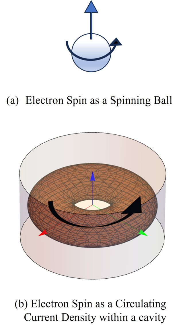
Figure 1: Figure (a) illustrates the conventional particle-spin model, depicting the electron as a rotating corpuscular ball. In contrast, Figure (b) presents a three-dimensional contour plot of the current density for the ground state $(101)$ electron, confined in a cylindrical cavity with radius $R=8~\text{nm}$, height $d=4~\text{nm}$, and potential energy $U=10~\text{meV}$. The contour is drawn at two-thirds of the peak current density, revealing a toroidal topology circulating around the $z$-axis. The corresponding eigenenergy is $\mathcal{E}_{101}-m_{e}c^{2}=8.06~\text{meV}$.

III Electron wave-spin qubit

The electron spin qubit is represented as a superposition of the spin-up and spin-down states, expressed by Eq. 16 and 17:

$$\psi=\cos\frac{\Theta}{2}\psi_{\uparrow}+\sin\frac{\Theta}{2}e^{i\Phi}\psi_{\downarrow},$$ (25)

where $0\leq\Theta\leq\pi$ and $0\leq\Phi\leq 2\pi$ uniquely define the qubit’s state. The parameter $\Theta$ controls the amplitude distribution between the spin-up and spin-down components, satisfying the normalization condition $\cos^{2}\frac{\Theta}{2}+\sin^{2}\frac{\Theta}{2}=1$. The relative phase $\Phi$ governs the quantum interference between the two states. Together, $\Theta$ and $\Phi$ determine the qubit’s position on the Bloch sphere[19], with logical operations represented as rotations on this sphere [12].

The relative phase $\Phi$ plays a central role in quantum computing. In the Quantum Fourier Transform (QFT)[20, 21], relative phases accumulate and encode periodicity in the amplitudes, enabling efficient solutions to problems like factoring in Shor’s algorithm[22]. In Grover’s search algorithm [23], constructive and destructive interference driven by phase inversion amplifies the correct solution. More generally, quantum phase manipulation is central to algorithms in quantum information science [24] such as Deutsch–Jozsa [25]. In our framework, this significance is made manifest through the current density and its corresponding magnetic field, both of which directly link to the relative phase $\Phi$ of the spin qubit.

The full wavefunction of the spin qubit follows directly from combining Eqs. 16,17, and Eq. 25:

$$\psi=\bBigg@{4.5}\{\begin{array}[]{cc}N\left(\begin{array}[]{c}\cos\frac{\Theta}{2}J_{0}(\zeta\rho)\cos(kz)\\ \sin\frac{\Theta}{2}e^{i\Phi}J_{0}(\zeta\rho)\cos(kz)\\ -i\cos\frac{\Theta}{2}\eta kJ_{0}(\zeta\rho)\sin(kz)-i\sin\frac{\Theta}{2}e^{i\Phi}\eta e^{-i\phi}\zeta J_{1}(\zeta\rho)\cos(kz)\\ -i\cos\frac{\Theta}{2}\eta e^{i\phi}\zeta J_{1}(\zeta\rho)\cos(kz)+i\sin\frac{\Theta}{2}e^{i\Phi}\eta kJ_{0}(\zeta\rho)\sin(kz)\\ \end{array}\right)&\text{Region I}\\ \\ \kappa N\left(\begin{array}[]{c}\cos\frac{\Theta}{2}K_{0}(\xi\rho)\cos(kz)\\ \sin\frac{\Theta}{2}e^{i\Phi}K_{0}(\xi\rho)\cos(kz)\\ -i\cos\frac{\Theta}{2}\eta kK_{0}(\xi\rho)\sin(kz)-i\sin\frac{\Theta}{2}e^{i\Phi}\eta e^{-i\phi}\xi K_{1}(\xi\rho)\cos(kz)\\ -i\cos\frac{\Theta}{2}\eta e^{i\phi}\xi K_{1}(\xi\rho)\cos(kz)+i\sin\frac{\Theta}{2}e^{i\Phi}\eta kK_{0}(\xi\rho)\sin(kz)\\ \end{array}\right)&\text{Region 1I}\end{array},$$ (26)

from which we can compute the current densities in each coordinate:

$$j_{\rho}=\Big{\{}\begin{array}[]{cc}-N^{2}ec\eta\sin\Theta\sin(\Phi-\phi)kJ_{0}(\zeta\rho)^{2}\sin(2kz),&\text{I}\\ -\kappa^{2}N^{2}ec\eta\sin\Theta\sin(\Phi-\phi)kK_{0}(\xi\rho)^{2}\sin(2kz),&\text{II}\end{array};$$ (29)

$$j_{\phi}=\Big{\{}\begin{array}[]{cc}-2N^{2}ec\eta\cos\Theta\zeta J_{0}(\zeta\rho)J_{1}(\zeta\rho)\cos^{2}(kz)+N^{2}ec\eta\sin\Theta\cos(\Phi-\phi)kJ_{0}(\zeta\rho)^{2}\sin(2kz),&\text{I}\\ -\kappa^{2}2N^{2}ec\eta\cos\Theta\xi K_{0}(\xi\rho)K_{1}(\xi\rho)\cos^{2}(kz)+\kappa^{2}N^{2}ec\eta\sin\Theta\cos(\Phi-\phi)kK_{0}(\xi\rho)^{2}\sin(2kz),&\text{II}\end{array};$$ (32)

$$j_{z}=\Big{\{}\begin{array}[]{cc}2N^{2}ec\eta\sin\Theta\sin(\Phi-\phi)\zeta J_{0}(\zeta\rho)J_{1}(\zeta\rho)\cos^{2}(kz),&\text{I}\\ \kappa^{2}2N^{2}ec\eta\sin\Theta\sin(\Phi-\phi)\xi K_{0}(\xi\rho)K_{1}(\xi\rho)\cos^{2}(kz),&\text{II}\end{array}.$$ (35)

In the special case where $\Theta=\frac{\pi}{2}$, corresponding to an equal superposition of spin-up and spin-down states, the current density simplifies to:

$$j_{\rho}=\Big{\{}\begin{array}[]{cc}-N^{2}ec\eta\sin(\Phi-\phi)kJ_{0}(\zeta\rho)^{2}\sin(2kz),&\text{I}\\ -\kappa^{2}N^{2}ec\eta\sin(\Phi-\phi)kK_{0}(\xi\rho)^{2}\sin(2kz),&\text{II}\end{array};$$ (39)

$$j_{\phi}=\Big{\{}\begin{array}[]{cc}N^{2}ec\eta\cos(\Phi-\phi)kJ_{0}(\zeta\rho)^{2}\sin(2kz),&\text{I}\\ \kappa^{2}N^{2}ec\eta\cos(\Phi-\phi)kK_{0}(\xi\rho)^{2}\sin(2kz),&\text{II}\end{array};$$ (42)

$$j_{z}=\Big{\{}\begin{array}[]{cc}2N^{2}ec\eta\sin(\Phi-\phi)\zeta J_{0}(\zeta\rho)J_{1}(\zeta\rho)\cos^{2}(kz),&\text{I}\\ \kappa^{2}2N^{2}ec\eta\sin(\Phi-\phi)\xi K_{0}(\xi\rho)K_{1}(\xi\rho)\cos^{2}(kz),&\text{II}\end{array}.$$ (45)

Notably, the current density depends on the difference between the relative phase $\Phi$ and the azimuthal angle. This means that the relative phase, an abstract parameter on the Bloch sphere, manifests physically in real space through the observable current densities. Specifically, the components of the current density, $j_{\rho}$ and $j_{\phi}$, are proportional to the vector $(\sin(\Phi-\phi),\cos(\Phi-\phi))$ in cylindrical coordinate. As a result, the current density in the $x-y$ plane points in the direction perpendicular to $\phi=\Phi$. Thus, the relative phase $\Phi$ directly determines the orientation of the current density, and together with the parameter $\Theta$, determines the overall configuration of the current density.

This real-space manifestation of the qubit is visualized through a three-dimensional contour plot of the current density, shown in Fig.2(b). The current circulates around an axis aligned with the direction $\phi=\Phi$, making the physical influence of the relative phase explicit. From the wave-entity perspective, the superposition of the spin states does not produce a ”Schrödinger’s cat”-like paradox, as illustrated in Fig.2(a), but instead results in a coherent and well-defined configuration of current density.

The wave-spin model further reveals that the qubit extends beyond the cavity as an evanescent wave, indicating that quantum information is not entirely confined within the physical boundary. In the following section, we show that the magnetic field generated by the qubit also penetrates into the surrounding space. This spatial extension of both the electron wave and its associated fields highlights the inherent connectivity among quantum systems. Crucially, this interdependence arises naturally from the wave dynamics, without requiring ”nonlocal” phenomena to explain quantum correlations or information transfer.

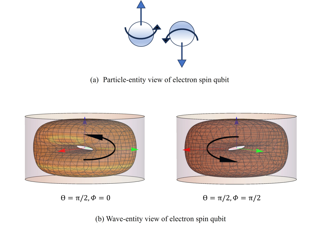
Figure 2: Figure (a) illustrates the particle-spin interpretation of a qubit, represented as a corpuscular ball spinning simultaneously up and down. In contrast, Figure (b) shows three-dimensional contour plots of the current density for the wave-spin qubit, $\psi=\cos\frac{\Theta}{2}\psi_{\uparrow}+\sin\frac{\Theta}{2}e^{i\Phi}\psi_{\downarrow}$, with $\Theta=\frac{\pi}{2}$. The contours are drawn at two-thirds of the peak current density, revealing toroidal topologies circulating around $\phi=\Phi=0$ ($x$-axis,red) and $\phi=\Phi=\frac{\pi}{2}$ ($y$-axis, green). These configurations demonstrate distinct phase-dependent nature of the wave-spin qubit. The electron is confined within a cylindrical cavity of radius $R=8~\text{nm}$, height $d=4~\text{nm}$, and potential energy $U=10~\text{meV}$. The spin-up and spin-down components are degenerate at the ground state $(nlm=101)$, with eigenenergy $\mathcal{E}_{101}-m_{e}c^{2}=8.06~\text{meV}$.

IV Magnetic field generated by wave-spin qubit

We demonstrate that a spin qubit can be characterized directly in physical space through its associated current density, rather than merely as a point on the abstract Bloch sphere. Each spin state corresponds to a unique, spatially extended current distribution, which, in principle, can be probed electromagnetically via interactions of the form $\boldsymbol{j}\cdot\boldsymbol{A}$. With appropriately engineered vector potentials ($\boldsymbol{A}$), these current profiles can be interrogated without collapsing the qubit into a particular quantum state, in a manner analogous to perturbative light–matter interactions.

More significantly, this current density generates a real magnetic field, deterministically and in accordance with Ampère’s law. While a full quantum-field treatment falls under the scope of Quantum Electrodynamics (QED), it is well justified, especially in mesoscopic systems, to calculate electromagnetic fields using Eq.1 or the Biot–Savart law[26], treating the quantum current as the source [27, 28, 29]. In this framework, quantum mechanics and classical electrodynamics intersect directly: electromagnetic fields emerge from the quantum current just as they do from classical sources. This is grounded in our interpretation of the electron wave as a spatially extended, real entity that intrinsically carries charge and current.

The resulting vector potential is given by:

$$\boldsymbol{A}(\boldsymbol{r})=\frac{\mu_{0}}{4\pi}\int\frac{\boldsymbol{j}(\boldsymbol{r^{\prime}})}{\left|\boldsymbol{r}-\boldsymbol{r^{\prime}}\right|}d^{3}\boldsymbol{r^{\prime}},$$ (47)

and the associated magnetic field follows from the Biot-Savart law:

$$\boldsymbol{B}(\boldsymbol{r})=\boldsymbol{\nabla}\times\boldsymbol{A}(\boldsymbol{r})=\frac{\mu_{0}}{4\pi}\int\boldsymbol{j}(\boldsymbol{r^{\prime}})\times\frac{\boldsymbol{r}-\boldsymbol{r^{\prime}}}{\left|\boldsymbol{r}-\boldsymbol{r^{\prime}}\right|^{3}}d^{3}\boldsymbol{r^{\prime}}.$$ (48)

Crucially, this formulation leads to a testable prediction: the magnetic field produced by a spin qubit is spatially asymmetric and explicitly dependent on the quantum state’s relative phase $\Phi$—a behavior absent in the particle-based model. We numerically evaluate this field for a qubit in the state $\Theta=\frac{\pi}{2}$ and $\Phi=\frac{\pi}{2}$, confined within the cylindrical geometry previously described. As shown in Fig.3, the magnetic field is oriented along $\phi=\Phi$ and extends beyond the confinement region into free space. Its magnitude, on the order of microtesla, falls within the sensitivity range of modern nanoscale magnetometers, such as nitrogen-vacancy (NV) centers in diamond[30, 31] and high-sensitivity Hall probes [32, 33].

This magnetic field serves not only as a direct experimental signature of the wave-entity interpretation but also as a medium for long-range, phased-mediated interactions between qubits. For example, a spatially arranged qubit array can exhibit global correlations: adjusting the relative phase of a single qubit may induce collective responses across the network. This mechanism provides a natural foundation for parallel quantum computing architectures, such as quantum cellular automata (QCA)[34, 35] and neuromorphic quantum computing[36, 37].

In contrast, the particle-based quantum mechanical framework treats the electron as a structureless point entity, endowed with angular momentum $\boldsymbol{S}$ and an associated magnetic dipole moment:

$$\boldsymbol{\mu}=-g\mu_{B}\frac{\boldsymbol{S}}{\hbar},$$ (49)

where $g\approx 2$ is the spin $g$-factor and $\mu_{B}$ is the Bohr magneton. The resulting magnetic field is:

$$\boldsymbol{B}(\boldsymbol{r})=\frac{\mu_{0}}{4\pi}\frac{3(\boldsymbol{\mu}\cdot\hat{\boldsymbol{r}})\hat{\boldsymbol{r}}-\boldsymbol{\mu}}{r^{3}},$$ (50)

which is azimuthally symmetric and independent of the phase parameter of the qubit. Significantly, a qubit in an equatorial state ($\Theta=\frac{\pi}{2}$) generates a negligible net magnetic field, as the dipole moment contributions cancel each other out.

Thus, the difference in the magnetic fields predicted by the wave-based and particle-based models offers a concrete test for distinguishing between competing interpretations of quantum mechanics.

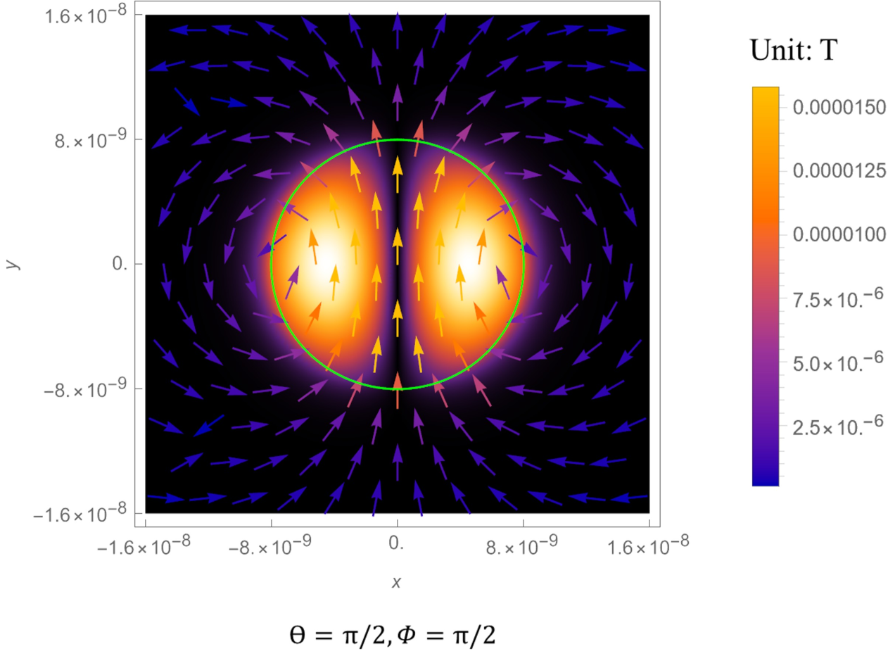
Figure 3: Vector plot of the magnetic field generated by the wave-spin qubit in the $z=0$ plane, overlaid on the corresponding current density. The qubit is in the state $\psi=\cos\frac{\Theta}{2}\psi_{\uparrow}+\sin\frac{\Theta}{2}e^{i\Phi}\psi_{\downarrow}$ with $\Theta=\frac{\pi}{2}$ and $\Phi=\frac{\pi}{2}$. The electron is confined within a cylindrical cavity of radius $R=8~\text{nm}$ (outlined in green), height $d=4~\text{nm}$, and potential energy $U=10~\text{meV}$. The spin-up and spin-down components are degenerate at the ground state $(nlm=101)$, with eigenenergy $\mathcal{E}_{101}-m_{e}c^{2}=8.06~\text{meV}$. The magnetic field is concentrated around the azimuthal direction $\phi=\Phi=\frac{\pi}{2}$ ($y$-axis), with the magnitude represented by the color scale.

V Conclusions and Limitations

In the framework where the electron is treated as a fundamental wave-entity, we propose that a spin qubit corresponds to a specific, physically real configuration of current density. This interpretation addresses Schrödinger’s cat-like paradoxes of superposition, avoiding the conceptual paradox of a particle spinning both up and down simultaneously.

We show that the relative phase between qubit basis states determines the orientation of the current density, thereby translating what is traditionally considered an abstract quantum parameter into a concrete, physically meaningful quantity.

The magnetic field predicted to emerge from such a wave-spin qubit differs markedly from the dipole fields associated with particle-based or probabilistic-wave interpretations. It is spatially asymmetric, strongly phase-dependent, and its field strength is predicted to reach the microtesla range, which places it within the detection capabilities of current magnetometry and qubit–qubit coupling techniques. These distinctive features provide clear avenues for experimental testing of the wave-entity model.

This phase-sensitive magnetic structure further suggests a mechanism for inherently parallel, phase-driven quantum computing architectures, offering an alternative to conventional, sequential gate-based logic. Intriguingly, such dynamics may share structural parallels with those observed in biological neural systems.

By treating the electron wave as the sole physical entity, we outline a quantum mechanical framework that is deterministic, local, and causal—reconciling the conceptual divide between quantum and classical physics.

As this model is theoretical and exploratory in nature, its conclusions remain provisional pending experimental validation. We encourage experimental efforts to investigate the predictions presented here and to explore the broader implications of the wave-entity perspective. This work is intended to initiate constructive scientific dialogue, attract critical peer feedback, and contribute to a deeper and more coherent understanding of the quantum world.

VI Acknowledgement

The authors gratefully acknowledge the insightful comments and constructive feedback provided by the reviewers on the Qeios platform in response to our previous work.

References

- Jackson [1999] J. D. Jackson, Classical Electrodynamics (Third edition. New York : Wiley, 1999, 1999).
- Jönsson [1961] C. Jönsson, Elektroneninterferenzen an mehreren künstlich hergestellten feinspalten, Zeitschrift für Physik 161, 454 (1961).
- Jönsson [1974] C. Jönsson, Electron diffraction at multiple slits, American Journal of Physics 42, 4 (1974), english translation of the 1961 German paper.
- Tonomura et al. [1989] A. Tonomura, J. Endo, T. Matsuda, T. Kawasaki, and H. Ezawa, Demonstration of single-electron buildup of an interference pattern, American Journal of Physics 57, 117 (1989).
- Davisson and Germer [1927] C. Davisson and L. H. Germer, Diffraction of electrons by a crystal of nickel, Physical Review 30, 705 (1927).
- Thomson and Reid [1927] G. P. Thomson and A. Reid, Diffraction of cathode rays by a thin film, Nature 119, 890 (1927).
- Dirac [1928] P. A. M. Dirac, Proceedings of the Royal Society A: Mathematical,Physical and Engineering Sciences 117, 610 (1928).
- Dirac [1930] P. A. M. Dirac, The Principles of Quantum Mechanics (Oxford University Press, 1930).
- Ohanian [1986] H. C. Ohanian, Am. J. Phys. 54, 6 (1986).
- Gao [2022] J. Gao, J. Phys. Commun. 6, 081001 (2022).
- Bohr [1928] N. Bohr, The quantum postulate and the recent development of atomic theory, Nature 121, 580 (1928).
- Nielsen and Chuang [2010] M. A. Nielsen and I. L. Chuang, Quantum Computation and Quantum Information, 10th ed. (Cambridge University Press, 2010).
- Schrödinger [1935] E. Schrödinger, Die gegenwärtige situation in der quantenmechanik, Naturwissenschaften 23, 807 (1935).
- Loss and DiVincenzo [1998] D. Loss and D. P. DiVincenzo, Quantum computation with quantum dots, Physical Review A 57, 120 (1998).
- Hanson et al. [2007] R. Hanson, L. P. Kouwenhoven, J. R. Petta, S. Tarucha, and L. M. K. Vandersypen, Spins in few-electron quantum dots, Reviews of Modern Physics 79, 1217 (2007).
- Gao and Shen [2024] J. Gao and F. Shen, Evanescent electron wave-spin, Entropy 26, 10.3390/e26090789 (2024).
- Lobanova and Ivanov [2004] O. R. Lobanova and A. I. Ivanov, (2004), arXiv:quant-ph/0411150 [quant-ph] .
- Unruh and Wald [2017] W. G. Unruh and R. M. Wald, Information loss, arXiv preprint arXiv:1703.02140 (2017).
- Bloch [1946] F. Bloch, Nuclear induction, Physical Review 70, 460 (1946).
- Cleve et al. [1998] R. Cleve, A. Ekert, C. Macchiavello, and M. Mosca, Quantum algorithms revisited, Proceedings of the Royal Society of London. Series A: Mathematical, Physical and Engineering Sciences 454, 339 (1998).
- Coppersmith [2002] D. Coppersmith, An approximate fourier transform useful in quantum factoring, arXiv preprint quant-ph/0201067 (2002).
- Shor [1999] P. W. Shor, Polynomial-time algorithms for prime factorization and discrete logarithms on a quantum computer, SIAM review 41, 303 (1999).
- Grover [1997] L. K. Grover, Quantum mechanics helps in searching for a needle in a haystack, Physical review letters 79, 325 (1997).
- Nielsen and Chuang [2002] M. A. Nielsen and I. L. Chuang, Quantum computation and quantum information, American Journal of Physics 70, 558 (2002), book review.
- Deutsch and Jozsa [1992] D. Deutsch and R. Jozsa, Rapid solution of problems by quantum computation, Proceedings of the Royal Society of London. Series A: Mathematical and Physical Sciences 439, 553 (1992).
- Biot and Savart [1820] J.-B. Biot and F. Savart, Loi relative au magnétisme produit par le courant électrique, Annales de Chimie et de Physique 20, 211 (1820).
- Imry [2002] Y. Imry, Introduction to Mesoscopic Physics, 2nd ed. (Oxford University Press, Oxford, 2002).
- Schwinger et al. [1998] J. Schwinger, K. A. Milton, L. L. J. DeRaad, W.-y. Tsai, and D. A. Sinha, Classical Electrodynamics (Westview Press, Boulder, CO, 1998).
- Datta [1995] S. Datta, Electronic Transport in Mesoscopic Systems (Cambridge University Press, Cambridge, 1995).
- Balasubramanian et al. [2008] G. Balasubramanian, I. Y. Chan, R. Kolesov, M. Al-Hmoud, W. Tittel, M. Reuter, F. Jelezko, and J. Wrachtrup, Nanoscale imaging magnetometry with diamond spins under ambient conditions, Nature 455, 648 (2008).
- Dreau et al. [2010] A. Dreau, Y. Kato, J. Dreau, T. Nishida, and H. Kosaka, Quantum sensing with nitrogen-vacancy centers in diamond, Physical Review B 81, 065303 (2010).
- Yousefi et al. [2012] H. Yousefi, M. Abdullah, C. Kueh, and M. Othman, Low-field magnetic sensing using a hall effect sensor for weak magnetic field detection, Journal of Magnetism and Magnetic Materials 324, 3461 (2012).
- Takemura et al. [2019] Y. Takemura, R. Asahi, Y. Hasegawa, and K. Furuya, Quantum hall sensors for ultra-sensitive magnetic field detection, Nature Communications 10, 4125 (2019).
- Watrous [1995] J. Watrous, On one-dimensional quantum cellular automata, Complex Systems 5, 19 (1995).
- Schumacher and Werner [2004] B. Schumacher and R. F. Werner, Reversible quantum cellular automata, arXiv preprint quant-ph/0405174 (2004).
- Marković et al. [2020] D. Marković, A. Mizrahi, D. Querlioz, and J. Grollier, Physics for neuromorphic computing, Nature Reviews Physics 2, 499 (2020).
- Behrman et al. [2000] E. C. Behrman, L. Nash, J. E. Steck, V. Chandrashekar, and S. R. Skinner, Quantum algorithm design using dynamic learning, Information Sciences 128, 257 (2000).