Real hyperelliptic solutions of gauged modified KdV equation of genus $g$

Abstract.

The real part of the focusing modified Korteweg-de Vries (MKdV) equation defined over the complex field ${\mathbb{C}}$ gives rise to the focusing gauged MKdV (FGMKdV) equation. In this paper, we construct the real hyperelliptic solutions of FGMKdV equation in terms of data of the hyperelliptic curves of genus $g$ by extending the previous results of genus three (Matsutani, Math. Phys. Ana. Geom. 27 (2024) 19).

Keywords: modified KdV equation, gauged modified KdV equation, real hyperelliptic solutions, hyperelliptic curves, focusing MKdV equation

1. Introduction

The modified Korteweg-de Vries (MKdV) equation is given by

$$\partial_{t}q\pm 6q^{2}\partial_{s}q+\partial_{s}^{3}q=0,$$ (1.1)

where $\partial_{t}:=\partial/\partial t$ and $\partial_{s}:=\partial/\partial s$ for the real axes $t$ and $s$. The “$+$”case in (1.1) is referred to as the focusing MKdV equation and the “$-$”case is referred to as the defocusing MKdV equation due to the [27]. The focusing MKdV equation appeared as an integrable system in geometry: By investigating an integrable system, Konno, Ichikawa and Wadati [9, 10], and Ishimori [11, 12] found plane curves that a half of their curvature $k/2$, ($k=\partial_{s}\phi$) obeys the focusing MKdV equation (1.1), i.e.,

$$\partial_{t}\phi+\frac{1}{2}(\partial_{s}\phi)^{3}+\partial_{s}^{3}\phi=0,$$ (1.2)

where $\phi$ is the tangential angle of the plane curve, which is known as the loop soliton. In this paper, we also call (1.2) the focusing modified KdV (FMKdV) equation, although we referred to (1.2) as the focusing modified pre-KdV equation in [17]. They showed that (1.2) can be regarded as a generalization of Euler’s elastica [9, 10, 11, 12].

Independently, Goldstein and Petrich showed that the isometric deformation of a real curve on a plane is connected with the recursion relations of the focusing MKdV hierarchy [7]. Following it, Previato and the author of this paper found that the Goldstein-Petrich scheme and the FMKdV equation [7] play an essential role in the isometric flows of the plane curves and in the statistical mechanics of the elasticae [25, 13, 23]. The excited states of the elasticae are described by the solutions of (1.2).

The paper [18] showed that finding the hyperelliptic solutions of the focusing MKdV equation of genus three based on the previous results [17] is critical to reproduce the shapes of supercoiled DNA in observed in laboratories. It provides a fascinating relationship between modern mathematics and life sciences. Thus, it is crucial to find the real hyperelliptic solutions of the FMKdV equation.

For a hyperelliptic curve $X$ of genus $g$ given by $y^{2}-(-1)^{g}(x-b_{0})(x-b_{1})\cdots(x-b_{2g})=0$ for $b_{i}\in{\mathbb{C}}$, due to Baker [1, 3, 6, 4, 21], we find the hyperelliptic solutions of the KdV equation as $\wp_{gg}(u)=x_{1}+\cdots+x_{g}$ for $((x_{1},y_{1}),\ldots,(x_{g},y_{g}))\in S^{g}X_{g}$ ($g$-th symmetric product of $X_{g}$) as a function of $u\in{\mathbb{C}}^{g}$ through the Abel-Jacobi map $v:S^{g}X_{g}\to J_{X}$ for the Jacobi variety $J_{X}$, $u=v((x_{1},y_{1}),\ldots,(x_{g},y_{g}))$. With the help of the Miura map it is not difficult to find the hyperelliptic solutions of the focusing MKdV equation over ${\mathbb{C}}$ [14], i.e.,

$$\partial_{u_{g-1}}\psi-\frac{1}{2}(\lambda_{2g}+3b_{0})\partial_{u_{g}}\psi+\frac{1}{8}\left(\partial_{u_{g}}\psi\right)^{3}+\frac{1}{4}\partial_{u_{g}}^{3}\psi=0,$$ (1.3)

where $\psi:=\log((b_{0}-x_{1})\cdots(b_{0}-x_{g}))/{\sqrt{-1}}$.

Let $a$-th component $u_{a}$ of $u\in{\mathbb{C}}^{g}$ be decomposed to its real and imaginary parts, $u_{a}=u_{a\,{\mathrm{r}}}+{\sqrt{-1}}u_{a\,{\mathrm{i}}}$, $\partial_{u_{a}}=\frac{1}{2}(\partial_{u_{a}\,{\mathrm{r}}}-{\sqrt{-1}}\partial_{u_{a}\,{\mathrm{i}}})$, $(a=1,\ldots,g)$, and let $\psi=\psi_{\mathrm{r}}+{\sqrt{-1}}\psi_{\mathrm{i}}$ of the real valued functions $\psi_{\mathrm{r}}$ and $\psi_{\mathrm{i}}$. The Cauchy-Riemann relations mean $\partial_{u_{a}\,{\mathrm{r}}}\psi_{{\mathrm{r}}}=\partial_{u_{a}\,{\mathrm{i}}}\psi_{{\mathrm{i}}}$ and $\partial_{u_{a}\,{\mathrm{r}}}\psi_{{\mathrm{i}}}=-\partial_{u_{a}\,{\mathrm{i}}}\psi_{{\mathrm{r}}}$, and thus $\partial_{u_{a}}\psi=\partial_{u_{a}\,{\mathrm{r}}}\psi_{{\mathrm{r}}}-{\sqrt{-1}}\partial_{u_{a}\,{\mathrm{i}}}\psi_{{\mathrm{r}}}$ or $\partial_{u_{a}}\psi=\partial_{u_{a}\,{\mathrm{r}}}(\psi_{{\mathrm{r}}}+{\sqrt{-1}}\psi_{{\mathrm{i}}})$ $(a=1,\ldots,g)$. Since (1.3) contains the cubic term $(\partial_{u_{g}}\psi)^{3}=(\partial_{u_{g}\,{\mathrm{r}}}\psi)^{3}$, it generates the term $-3(\partial_{u_{g}\,{\mathrm{r}}}\psi_{\mathrm{i}})^{2}\partial_{u_{g}\,{\mathrm{r}}}\psi_{\mathrm{r}}$, which behaves like a gauge potential. Thus we encounter coupled differential relations from the focusing MKdV equation over ${\mathbb{C}}$ (1.3) as

$$\begin{split}&(\partial_{u_{g-1}\,{\mathrm{r}}}-A^{+}(u)\partial_{u_{g}\,{\mathrm{r}}})\psi_{\mathrm{r}}+\frac{1}{8}\left(\partial_{u_{g}\,{\mathrm{r}}}\psi_{\mathrm{r}}\right)^{3}+\frac{1}{4}\partial_{u_{g}\,{\mathrm{r}}}^{3}\psi_{\mathrm{r}}=0,\\ &(\partial_{u_{g-1}\,{\mathrm{i}}}-A^{-}(u)\partial_{u_{g}\,{\mathrm{i}}})\psi_{\mathrm{r}}+\frac{1}{8}\left(\partial_{u_{g}\,{\mathrm{i}}}\psi_{\mathrm{r}}\right)^{3}+\frac{1}{4}\partial_{u_{g}\,{\mathrm{i}}}^{3}\psi_{\mathrm{r}}=0,\end{split}$$ (1.4)

where $A^{+}(u)=(\lambda_{2g}+3b_{a}+\frac{3}{4}(\partial_{u_{g}\,{\mathrm{r}}}\psi_{\mathrm{i}})^{2})/2$ and $A^{-}(u)=(\lambda_{2g}+3b_{a}-\frac{3}{4}(\partial_{u_{g}\,{\mathrm{r}}}\psi_{\mathrm{r}})^{2})/2$. We refer to (1.4) as the focusing gauged MKdV (FGMKdV) equations. Here we take both cases $(u_{g\,{\mathrm{r}}},u_{g-1\,{\mathrm{r}}})\in{\mathbb{R}}^{2}$ and ${\sqrt{-1}}(u_{g\,{\mathrm{i}}},u_{g-1\,{\mathrm{i}}})$ in ${\sqrt{-1}}{\mathbb{R}}^{2}$ in (1.4).

[24] gave that to obtain the real solution of focusing MKdV equation (1.2) is to find the situation that the following conditions are satisfied for the solutions of (1.4):

1. $\prod_{i=1}^{g}|x_{i}-b_{a}|=$ a constant $(>0)$,

2. $du_{g\,{\mathrm{i}}}=du_{g-1\,{\mathrm{i}}}=0$ or $du_{g\,{\mathrm{r}}}=du_{g-1\,{\mathrm{r}}}=0$, and

3. $A^{\pm}(u)$ is a real constant: if $A^{\pm}(u)=$ constant, (1.4) is reduced to (1.2), i.e., $\psi_{\mathrm{r}}=\phi$.

However, it is quite difficult to find the real plane $\{(u_{g},u_{g-1})\}$ in the Jacobi variety $J_{X}$ which corresponds to the preimage $((x_{1},y_{1}),\ldots,(x_{g},y_{g}))\in S^{g}X$ of $v$ with the unit circle valued ${\mathrm{e}}^{{\sqrt{-1}}\psi}=(b_{0}-x_{1})\cdots(b_{0}-x_{g})\in\mathrm{U}(1):=\{\zeta\in{\mathbb{C}}\ |\ |\zeta|=1\}$.

In the previous papers [17, 20], we showed the real hyperelliptic solutions of the FGMKdV equation for the case of the genus three only by considering the conditions CI and CII.

This paper aims to extend the results for genus three in [17, 20] to the general genera $g$. We will show that the extension is naturally achieved by investigating the angle expressions of the hyperelliptic integrals in [16] as in Section 3, and a modification of the elementary symmetric polynomials. We refer to the modification of the elementary symmetric polynomials as shifted elementary symmetric polynomials in this paper, which are mentioned in Appendix.

The symmetric polynomials determine a fundamental property of the Jacobi matrices between the cotangent spaces $T^{*}S^{g}X$ and $T^{*}J_{X}$ of $S^{g}X$ and $J_{X}$, respectively. Weierstrass and Baker essentially studied the correspondence between $T^{*}S^{g}X$ and $T^{*}J_{X}$ to obtain the differential identities on hyperelliptic curves of genus $g$, which are related to the sine-Gordon equation and the KdV hierarchy. They implicitly and explicitly used the elementary symmetric polynomials. (Recently, such a picture is sophisticated from a modern point of view and extended by Buchstaber and Mikhailov [5, 6].)

In this paper, we apply their method to the configurations satisfying the condition CI or $(b_{0}-x_{1})\cdots(b_{0}-x_{g})\in\mathrm{U}(1)$ to obtain the real FGMKdV equation as a real differential identities of genus $g$, although we implicitly employed this approach in [17, 20] for the genus three case. On the extension from genus three to the general genus $g$, the properties of the shifted elementary symmetric polynomials are essential. We show them in Appendix.

The content is following: Section 2 reviews the hyperelliptic solutions of the focusing MKdV equation over ${\mathbb{C}}$ of genus $g$ in Theorem 2.3 following [15, 22, 24] for the hyperelliptic curve $X$ of genus $g$. Since the real solutions are related to the covering ${\widehat{X}}$ of $X$ and the angle expression, Section 3 is devoted to the double covering ${\widehat{X}}$ of $X$ and the angle expression of the hyperelliptic curves of genus $g$. Section 4 provides local properties of the solutions of the FGMKdV equation (1.4) as in Theorem 4.7. To obtain the real hyperelliptic solutions of the FGMKdV equation, we employ the Assumptions 3.1 and 3.9. Based on these, we also show the global behavior of the hyperelliptic solutions of genus $g$ of the gauged MKdV equation in Theorem 4.8. Theorems 4.7 and 4.8 are our main theorems, showing that we have the real solutions of the FGMKdV equation of genus $g>2$. Section 5 gives the conclusion of this paper. Since Lemmas 3.7, 4.1 and 4.5 are key lemmas in this paper but their proofs are very complicated, we prepare Appendix to show their proofs. In Appendix, the proofs are associated with shifted elementary symmetric polynomials.

2. Hyperelliptic solutions of the focusing MKdV equation$/{\mathbb{C}}$ of genus $g$

To obtain the relation (1.3), we handle a hyperelliptic curve $X$ of genus $g\geq 3$ over ${\mathbb{C}}$,

$$X=\left\{(x,y)\in{\mathbb{C}}^{2}\ |\ y^{2}-(-1)^{g}f(x)=0\right\}\cup\{\infty\},$$ (2.1)

where $f(x):=(x-b_{0})(x-b_{1})(x-b_{2})\cdots(x-b_{2g})$, and $b_{i}$’s are mutually distinct complex numbers. Let $\lambda_{2g}=\displaystyle{-\sum_{i=0}^{2g}b_{i}}$ and $S^{k}X$ be the $k$-th symmetric product of the curve $X$. Further, we introduce the Abelian covering ${\widetilde{X}}$ of $X$ by abelianization of the path-space of $X$ divided by the homotopy equivalence, $\kappa_{X}:{\widetilde{X}}\to X$, ($\gamma_{P,\infty}\mapsto P$) [2, 26, 22, 21]. Here $\gamma_{P,\infty}$ means a path from $\infty$ to $P$. We also consider an embedding $\iota_{X}:X\to{\widetilde{X}}$ and will fix it. $S^{k}{\widetilde{X}}$ also means the $k$-th symmetric product of the space ${\widetilde{X}}$. The Abelian integral ${\widetilde{v}}:=\displaystyle{\begin{pmatrix}v_{1}\\ \vdots\\ v_{g}\end{pmatrix}}:S^{g}{\widetilde{X}}\to{\mathbb{C}}^{g}$ is defined by

$${\widetilde{v}}_{i}(\gamma_{1},\ldots,\gamma_{g})=\sum_{j=1}^{g}{\widetilde{v}}_{i}(\gamma_{j}),\quad{\widetilde{v}}_{i}(\gamma_{(x,y),\infty})=\int_{\gamma_{(x,y),\infty}}{\nu_{i}},\quad{\nu_{i}}=\frac{x^{i-1}dx}{2y}.$$ (2.2)

Then we have the Jacobian $J_{X}$, $\kappa_{J}:{\mathbb{C}}^{g}\to J_{X}={\mathbb{C}}^{g}/\Gamma_{X}$, where $\Gamma_{X}$ is the lattice generated by the period matrix for the standard homology basis of $X$. Due to the Abel-Jacobi theorem [8], we also have the bi-rational map $v$ from $S^{3}X$ to $J_{X}$ by letting $v:={\widetilde{v}}$ modulo $\Gamma_{X}$. We refer to $v$ as the Abel-Jacobi map.

[15] shows the hyperelliptic solutions of the MKdV equation over ${\mathbb{C}}$, derived by a natural extension of the investigations of Weierstrass [26] and Baker [3]. Recently these methods [26] and [3] are refined by Buchstaber and Mikhailov [5, 6].

Definition 2.1.

Let $\{(x_{i},y_{i})\}_{i=1,\ldots,g}\in S^{g}X$.

1. We define the polynomials associated with $F(x)=(x-x_{1})\cdots(x-x_{g})$ by

   $$\pi_{i}(x):=\frac{F(x)}{x-x_{i}}=\chi_{i,g-1}x^{g-1}+\chi_{i,g-2}x^{g-2}+\cdots+\chi_{i,1}x+\chi_{i,0}.$$ (2.3)

2. We define $g\times g$ matrices as follows.

   $${\mathcal{X}}:={\small{\left(\begin{array}[]{cccc}\chi_{1,0}&\chi_{1,1}&\cdots&\chi_{1,g-1}\\ \chi_{2,0}&\chi_{2,1}&\cdots&\chi_{2,g-1}\\ \vdots&\vdots&\ddots&\vdots\\ \chi_{g,0}&\chi_{g,1}&\cdots&\chi_{g,g-1}\end{array}\right)}},\quad{\mathcal{Y}}:={\small{\left(\begin{array}[]{cccc}y_{1}&&&\\ &y_{2}&&\\ &&\ddots&\\ &&&y_{g}\end{array}\right)}},$$

   $${\mathcal{F}}^{\prime}:={\small{\left(\begin{array}[]{cccc}F^{\prime}(x_{1})&&&\\ &F^{\prime}(x_{2})&&\\ &&\ddots&\\ &&&F^{\prime}(x_{g})\end{array}\right)}},\quad{\mathcal{U}}:={\small{\left(\begin{array}[]{cccc}1&1&\cdots&1\\ x_{1}&x_{2}&\cdots&x_{g}\\ x_{1}^{2}&x_{2}^{2}&\cdots&x_{g}^{2}\\ \vdots&\vdots&\ddots&\vdots\\ x_{1}^{g-1}&x_{2}^{g-1}&\cdots&x_{g}^{g-1}\end{array}\right)}},$$

   where $F^{\prime}(x):=dF(x)/dx$.

Using them, we have the following [3, 14]:

Lemma 2.2.

Let $u={\widetilde{v}}(\iota_{X}((x_{1},y_{1}),\ldots,(x_{g},y_{g})))$.

1. $$\left[\begin{array}[]{c}du_{1}\\ du_{2}\\ \vdots\\ d{u_{g}}\end{array}\right]=\frac{1}{2}{\mathcal{U}}{\mathcal{Y}}^{-1}\left[\begin{array}[]{c}d{x_{1}}\\ d{x_{2}}\\ \vdots\\ d{x_{g}}\end{array}\right].$$

2. The inverse matrix of ${\mathcal{U}}$ is given as ${\mathcal{X}}$, i.e, ${\mathcal{X}}{\mathcal{U}}={\mathcal{F}}^{\prime}$.

3. For $\partial_{u_{i}}:=\partial/\partial{u_{i}}$ and $\partial_{x_{i}}:=\partial/\partial{x_{i}}$, we have

   $$\left[\begin{array}[]{c}\partial_{u_{1}}\\ \partial_{u_{2}}\\ \vdots\\ \partial_{u_{g}}\end{array}\right]=2{\mathcal{Y}}{\mathcal{F}}^{\prime-1}{\,{}^{t}\negthinspace}{\mathcal{X}}\left[\begin{array}[]{c}\partial_{x_{1}}\\ \partial_{x_{2}}\\ \vdots\\ \partial_{x_{g}}\end{array}\right],\quad\frac{\partial x_{i}}{\partial u_{r}}=\frac{2y_{i}}{F^{\prime}(x_{i})}\chi_{i,r-1},$$

   $$\frac{\partial}{\partial u_{g}}=\sum_{i=1}^{g}\frac{2y_{i}}{F^{\prime}(x_{i})}\frac{\partial}{\partial x_{i}},\quad\frac{\partial}{\partial u_{g-1}}=\sum_{i=1}^{g}\frac{2y_{i}\chi_{i,g-1}}{F^{\prime}(x_{i})}\frac{\partial}{\partial x_{i}}.$$ (2.4)

By applying these differential operator $\displaystyle{\frac{\partial}{\partial u_{g}}}$ and $\displaystyle{\frac{\partial}{\partial u_{g-1}}}$ to $\log F(b_{0})$, we obtain the following theorem.

Theorem 2.3.

[15] For $((x_{1},y_{1}),\cdots,(x_{g},y_{g}))\in S^{g}X$, the fixed branch point $(b_{0},0)$, and $u:=v((x_{1},y_{1}),$ $\cdots,(x_{g},y_{g}))$,

$${\psi(u):=-{\sqrt{-1}}\log(b_{0}-x_{1})(b_{0}-x_{2})\cdots(b_{0}-x_{g})}$$

satisfies the MKdV equation over ${\mathbb{C}}$,

$$(\partial_{u_{g-1}}-\frac{1}{2}(\lambda_{2g}+3b_{0})\partial_{u_{g}})\psi+\frac{1}{8}\left(\partial_{u_{g}}\psi\right)^{3}+\frac{1}{4}\partial_{u_{g}}^{3}\psi=0,$$ (2.5)

where $\partial_{u_{i}}:=\partial/\partial u_{i}$ as an differential identity in $S^{g}X$ and ${\mathbb{C}}^{g}$.

We, here, emphasize the difference between the focusing MKdV equations (1.2) over ${\mathbb{R}}$ and (2.5) over ${\mathbb{C}}$. In (1.2), $\phi$ is a real valued function over ${\mathbb{R}}^{2}$ but $\psi$ in (2.5) is a complex valued function over ${\mathbb{C}}^{2}\subset{\mathbb{C}}^{g}$. The difference is crucial since our ultimate goal is to obtain solutions of (1.2), not (2.5). However, the latter is expressed well in terms of the hyperelliptic function theory.

As mentioned in [24, (11)], we describe the difference. By introducing real and imaginary parts, $u_{a}=u_{a\,{\mathrm{r}}}+{\sqrt{-1}}u_{a\,{\mathrm{i}}}$, $(a=1,2,3)$, and $\psi=\psi_{{\mathrm{r}}}+{\sqrt{-1}}\psi_{{\mathrm{i}}}$, the real and imaginary part of (2.5) are reduced to the gauged MKdV equations with the gauge fields $A^{+}(u)=(\lambda_{2g}+3b_{a}+\frac{3}{4}(\partial_{u_{g}\,{\mathrm{i}}}\psi_{\mathrm{r}})^{2})/2$, $A^{-}(u)=(\lambda_{2g}+3b_{a}-\frac{3}{4}(\partial_{u_{g}\,{\mathrm{r}}}\psi_{\mathrm{r}})^{2})/2$,

$$(\partial_{u_{g-1}\,{\mathrm{r}}}-A^{+}(u)\partial_{u_{g}\,{\mathrm{r}}})\psi_{\mathrm{r}}+\frac{1}{8}\left(\partial_{u_{g}\,{\mathrm{r}}}\psi_{\mathrm{r}}\right)^{3}+\frac{1}{4}\partial_{u_{g}\,{\mathrm{r}}}^{3}\psi_{\mathrm{r}}=0,$$

$$(\partial_{u_{g-1}\,{\mathrm{i}}}-A^{-}(u)\partial_{u_{g}\,{\mathrm{i}}})\psi_{\mathrm{r}}+\frac{1}{8}\left(\partial_{u_{g}\,{\mathrm{i}}}\psi_{\mathrm{r}}\right)^{3}+\frac{1}{4}\partial_{u_{g}\,{\mathrm{i}}}^{3}\psi_{\mathrm{r}}=0$$ (2.6)

by the Cauchy-Riemann relations $\partial_{u_{a}\,{\mathrm{r}}}\psi_{{\mathrm{r}}}=\partial_{u_{a}\,{\mathrm{i}}}\psi_{{\mathrm{i}}}$ and $\partial_{u_{a}\,{\mathrm{r}}}\psi_{{\mathrm{i}}}=-\partial_{u_{a}\,{\mathrm{i}}}\psi_{{\mathrm{r}}}$ as mentioned in [24, (11)] and (1.4). We note that $\partial_{u_{a}}\psi=\partial_{u_{a}\,{\mathrm{i}}}(\psi_{{\mathrm{r}}}+{\sqrt{-1}}\psi_{{\mathrm{i}}})$ because $\partial_{u_{a}}=(\partial_{u_{a}\,{\mathrm{r}}}-{\sqrt{-1}}\partial_{u_{a}\,{\mathrm{i}}})/2$, and thus $(\partial_{u_{g}}\psi)^{3}$ contains the term $-3(\partial_{u_{g}\,{\mathrm{r}}}\psi_{{\mathrm{i}}})^{2}\partial_{u_{g}\,{\mathrm{r}}}\psi_{{\mathrm{r}}}$. We also note that the latter one has an alternative expression as defocusing gauged MKdV equation,

$$(\partial_{u_{g-1}\,{\mathrm{r}}}-A^{-}(u)\partial_{u_{g}\,{\mathrm{r}}})\psi_{\mathrm{i}}-\frac{1}{8}\left(\partial_{u_{g}\,{\mathrm{r}}}\psi_{\mathrm{i}}\right)^{3}+\frac{1}{4}\partial_{u_{g}\,{\mathrm{r}}}^{3}\psi_{\mathrm{i}}=0,$$ (2.7)

even though we will not touch this expression.

A solution of (1.2) in terms of the data in Theorem 2.3 must satisfy the following conditions [24]:

Condition 2.4.

1. $\prod_{i=1}^{g}|x_{i}-b_{a}|=$ a constant $(>0)$ in Theorem 2.3,

2. $du_{g\,{\mathrm{i}}}=du_{g-1\,{\mathrm{i}}}=0$ or $du_{g\,{\mathrm{r}}}=du_{g-1\,{\mathrm{r}}}=0$ in Theorem 2.3, and

3. $A(u)$ is a real constant: if $A(u)=$ constant (or $\partial_{u_{g}\,{\mathrm{r}}}\psi_{\mathrm{i}}=$ constant), (2.6) is reduced to (1.2), i.e., $\psi_{\mathrm{r}}=\phi$.

It is obvious that if we have the solutions $\psi_{\mathrm{r}}$ of (2.6) satisfying the conditions CI–CIII, $\partial_{u_{g},{\mathrm{r}}}\psi_{{\mathrm{r}}}/2$ obeys the focusing MKdV equation (1.1).

However, in this paper we focus on the conditions CI and CII and the real hyperelliptic solutions of the FGMKdV equation (2.6) of genus $g$ instead of (1.2).

3. Hyperelliptic curves of genus $g$ in angle expression

To find real solutions of the FGMKdV equation (2.6) under Condition 2.4 CI and CII, we introduce the angle expression [16, 24, 17, 20] for $X\setminus\{(b_{0},0)\}$ as mentioned in Introduction.

Since the angle expression is connected with a double covering ${\widehat{X}}$ of $X$, we introduce the double covering ${\widehat{X}}$ as in Figure 1. We consider the ${\mathrm{al}}_{a}(u)$ function $\sqrt{\prod_{i=1}^{g}(b_{a}-x_{i})}$ for a branch point $B_{a}:=(b_{a},0)\in X$ ($\varpi_{x}:X\to{\mathbb{P}}^{1}$) and $((x_{i},y_{i}))_{i}\in S^{g}X$. It means that we consider a line bundle on $X$ and its local section on an open set $U\subset X$. Here $u$ is given by $u:={\widetilde{v}}_{i}(\gamma_{1},\ldots,\gamma_{g})\in{\mathbb{C}}^{g}$ such that $\kappa_{X}(\gamma_{i})=(x_{i},y_{i})$. Fix $a=0$. The square root leads the transformation of $w^{2}=(x-b_{0})$, i.e., the double covering ${\widehat{X}}$ of the curve $X$, $\varpi_{\widehat{X}}:{\widehat{X}}\to X$, although the precise arguments are left to the Appendix in [22]. Since ${\widetilde{X}}$ is also a covering of ${\widehat{X}}$, we have a natural commutative diagram,

(3.1)

The ${\mathrm{al}}_{a}(u)$ function is a generalization of the Jacobi ${\mathrm{sn}},{\mathrm{cn}},{\mathrm{dn}}$ functions because the Jacobi function consists of $\sqrt{x-e_{i}}$, ($i=1,2,3$) of genus one for a curve $y^{2}=\prod_{i=1}^{3}(x-e_{i})$.

The curve ${\widehat{X}}$ is given by $f_{\widehat{X}}(w,z)=z^{2}-(-)^{g}(w^{2}-e_{1})\cdots(w^{2}-e_{2g})=0$, where $z:=y/w$ (due to normalization), and $e_{j}:=b_{j}-b_{0}$, $j=1,\ldots,2g$. Its affine ring is $R_{\widehat{X}}:={\mathbb{C}}[w,z]/(f_{\widehat{X}}(w,z))$, and the ring of its $g$-th symmetric polynomials is denoted by $S^{g}R_{\widehat{X}}$.

Since the genus of ${\widehat{X}}$ is $2g-1$, we have $2g-1$ holomorphic one-forms,

$${\widehat{\nu}}_{j}:=\frac{w^{j}dw}{z},\quad(j=1,2,3,\ldots,2g-1),$$

and the Jacobi variety, $J_{{\widehat{X}}}$ of ${\widehat{X}}$ is given by the complex torus $J_{{\widehat{X}}}={\mathbb{C}}^{2g-1}/\Gamma_{{\widehat{X}}}$ for the lattice $\Gamma_{{\widehat{X}}}$ generated by the period matrix. As in [22, Appendix, Proposition 11.9], we have the correspondence $\varpi_{X}^{*}{\nu_{i}}={\widehat{\nu}}_{2i-2}$, $(i=1,\ldots,g)$ and thus the Jacobian $J_{{\widehat{X}}}$ contains a subvariety ${\widehat{J}}_{X}\subset J_{{\widehat{X}}}$ which is a double covering of the Jacobian $J_{X}$ of $X$, ${\widehat{\varpi}}_{J}:{\widehat{J}}_{X}\to J_{X}$, and ${\widehat{\kappa}}_{J}:{\mathbb{C}}^{g}\to{\widehat{J}}_{X}:={\mathbb{C}}^{g}/(\Gamma_{\widehat{X}}\cap{\mathbb{C}}^{g})$.

Since for each branch point $B_{j}:=(b_{j},0)\in X$ $(j=1,\ldots,2g)$, we have double branch points ${\widehat{B}}^{\pm}_{j}:=(\pm\sqrt{e_{j}},0)\in{\widehat{X}}$ as illustrated in Figure 1.

Similar to the Jacobi elliptic functions, ${\widehat{J}}_{X}={\mathbb{C}}^{g}/{\widehat{\Gamma}}_{X}$ is determined by the same Abelian integral ${\widetilde{v}}$, and thus we use the same symbol ${\widetilde{v}}$ as ${\widetilde{v}}:S^{g}{\widetilde{X}}\to{\mathbb{C}}^{g}$ for ${\widehat{X}}$ [22].

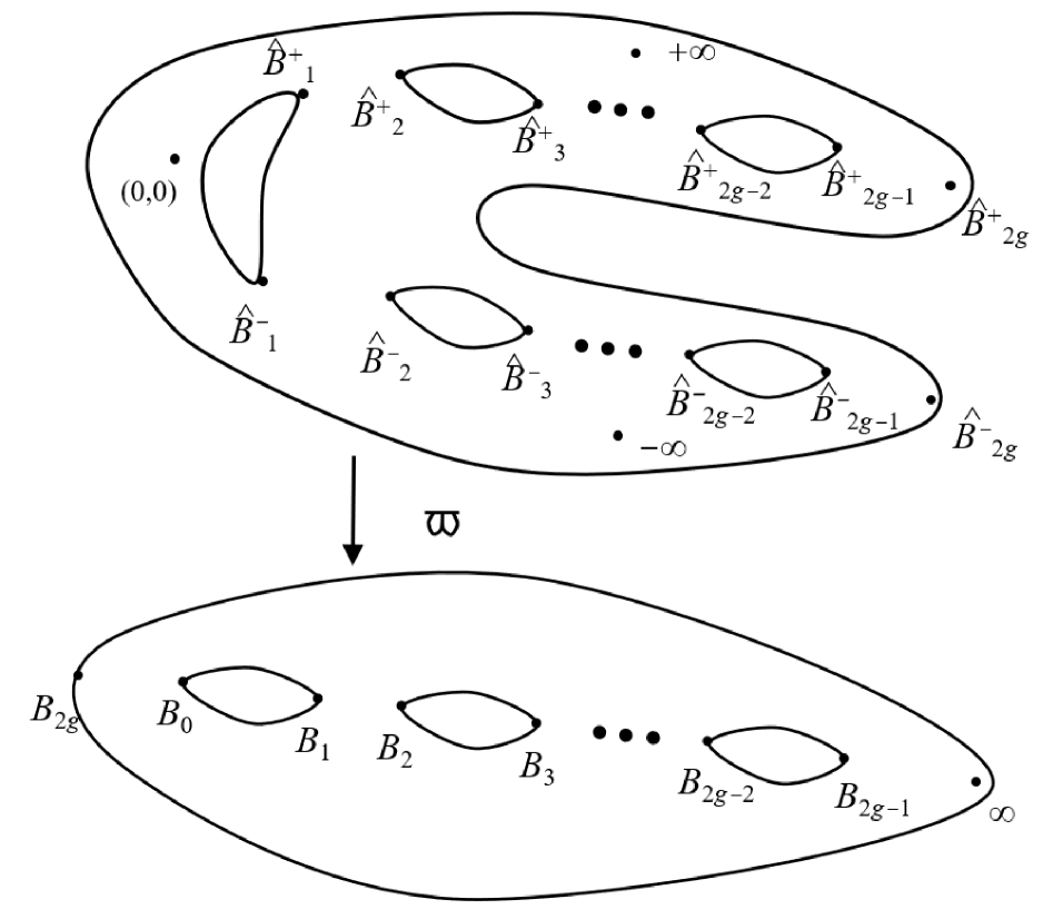
Figure 1. The double covering $\varpi_{\widehat{X}}:{\widehat{X}}\to X$, $\varpi_{X}:(w,z)\mapsto(w^{2}+b_{0},zw)=(x,y)$.

We restrict the moduli (rather, parameter) space of the curve $X$ by the following. We choose coordinates $u={}^{t}(u_{1},\ldots,u_{g})$ in ${\mathbb{C}}^{g}$; $u_{i}=u_{i}^{(1)}+u_{i}^{(2)}+\cdots+u_{i}^{(g)}$, where $u_{i}^{(j)}=v_{i}((x_{j},y_{j}))$ for $(x_{j},y_{j})\in X$. There are the projection $\varpi_{x}:X\to{\mathbb{P}}^{1}$, $((x,y)\mapsto x)$, and similarly ${\widehat{\varpi}}_{x}:{\widehat{X}}\to{\mathbb{P}}^{1}$, $((w,z)\mapsto w)$; ${\widehat{\varpi}}_{x}=\varpi_{x}\circ\varpi_{\widehat{X}}$.

Assumption 3.1.

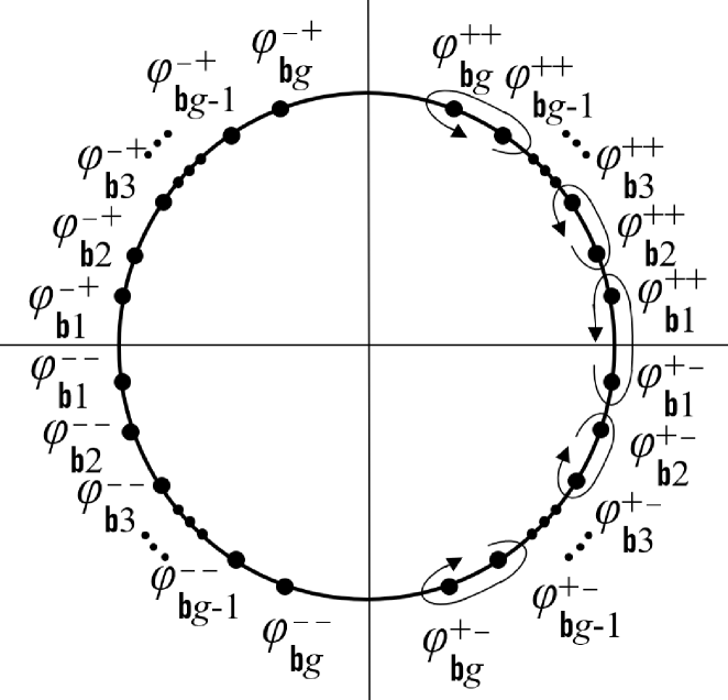
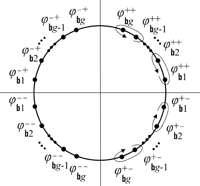
(a)                 (b)

Figure 2. ${\mathcal{A}}_{X}\subset S^{1}$: $k_{1}>k_{2}>\cdots>k_{g}>1.0$ for the odd $g$ (a) and the even $g$ (b).

As in Figure 2, we let $e_{j}:=b_{j}-b_{0}$, $(j=1,2,\ldots,2g)$ be on a unit circle $\mathrm{U}(1)=S^{1}$ whose center is the origin $b_{0}$ such that $e_{2i-1}=\overline{e_{2i}}$, $(i=1,2,\ldots,g)$; there are $\varphi_{{\mathfrak{b}},i}^{++}$, $(i=1,2,\ldots,g)$ such that

$$e_{2i-1}=e^{2{\sqrt{-1}}\varphi_{{\mathfrak{b}},i}^{++}},\quad e_{2i}=e^{-2{\sqrt{-1}}\varphi_{{\mathfrak{b}},i}^{++}},\quad(i=1,2,\ldots,g).$$

We let $\varphi_{{\mathfrak{b}},i}^{+-}:=-\varphi_{{\mathfrak{b}},i}^{++}$, and $\varphi_{{\mathfrak{b}},i}^{-\pm}:=\pi\mp\varphi_{{\mathfrak{b}},i}^{++}$. Further, we rename them as

1. $g$ odd case: $\varphi_{{\mathfrak{b}}}^{[1\pm]}:=\varphi_{{\mathfrak{b}},1}^{+\pm}$

   $$\varphi_{{\mathfrak{b}}}^{[\ell+]}:=\varphi_{{\mathfrak{b}},2\ell-1}^{++},\ \varphi_{{\mathfrak{b}}}^{[\ell-]}:=\varphi_{{\mathfrak{b}},2\ell-2}^{++},\ (\ell=2,3,\cdots,(g+1)/2),$$

   $$\varphi_{{\mathfrak{b}}}^{[(\ell+(g-1)/2+)]}:=\varphi_{{\mathfrak{b}},2\ell-2}^{+-},\ \varphi_{{\mathfrak{b}}}^{[(\ell+(g-1)/2-)]}:=\varphi_{{\mathfrak{b}},2\ell-1}^{+-},\ (\ell=2,3,\cdots,(g+1)/2),$$

   $${\mathcal{A}}_{X}:=\{{\mathrm{e}}^{{\sqrt{-1}}\varphi}\ |\ \varphi\in{\mathcal{A}}_{X}^{\varphi}\},\qquad{\mathcal{A}}_{X}^{\varphi}:=\bigcup_{\ell=1}^{2g}[\varphi_{{\mathfrak{b}}}^{[\ell-]},\varphi_{{\mathfrak{b}}}^{[\ell+]}].$$ (3.2)

2. $g$ even case:

   $$\varphi_{{\mathfrak{b}}}^{[\ell+]}:=\varphi_{{\mathfrak{b}},2\ell}^{++},\ \varphi_{{\mathfrak{b}}}^{[\ell-]}:=\varphi_{{\mathfrak{b}},2\ell-1}^{++},\ (\ell=1,2,\cdots,g/2),$$

   $$\varphi_{{\mathfrak{b}}}^{[(\ell+g/2)+]}:=\varphi_{{\mathfrak{b}},2\ell-1}^{+-},\ \varphi_{{\mathfrak{b}}}^{[(\ell+g/2)-]}:=\varphi_{{\mathfrak{b}},2\ell}^{+-},\ (\ell=1,2,\cdots,g/2),$$

   $${\mathcal{A}}_{X}:=\{{\mathrm{e}}^{{\sqrt{-1}}\varphi}\ |\ \varphi\in{\mathcal{A}}_{X}^{\varphi}\},\qquad{\mathcal{A}}_{X}^{\varphi}:=\bigcup_{\ell=1}^{2g}[\varphi_{{\mathfrak{b}}}^{\ell-},\varphi_{{\mathfrak{b}}}^{\ell+}].$$ (3.3)

We recall $w^{2}=(x-b_{0})$ and $w={\mathrm{e}}^{{\sqrt{-1}}\varphi}\in{\widehat{X}}\setminus\{(0,0)\}$. For a ‘real’ expression of (2.1), we use the following transformation, which is a generalization of ‘the angle expression’ of the elliptic integral as mentioned in [24].

Lemma 3.2.

$(w^{2}-e_{1})(w^{2}-e_{2})=4\frac{1}{k_{1}^{2}}{\mathrm{e}}^{2{\sqrt{-1}}\varphi}(1-k^{2}\sin^{2}\varphi)$, where

$$w={\mathrm{e}}^{{\sqrt{-1}}\varphi},\quad k_{1}=\frac{2{\sqrt{-1}}\sqrt[4]{e_{1}e_{2}}}{\sqrt{e_{1}}-\sqrt{e_{2}}}=\frac{1}{\sin\varphi_{{\mathfrak{b}}1}^{++}},\quad e_{1}e_{2}=1.$$

Proof.

Let $e_{1}e_{2}=1$. We recall the double angle formula $\cos 2\varphi=1-2\sin^{2}\varphi$.

$$\begin{split}(w^{2}-e_{1})(w^{2}-e_{2})&=w^{2}(w^{2}-(e_{1}+e_{2})+e_{1}e_{2}w^{-2})\\ &=2w^{2}\left(\cos(2\varphi)-\frac{e_{1}+e_{2}}{2}\right)\\ &=-w^{2}\left(e_{1}+e_{2}-2\sqrt{e_{1}e_{2}}+4\sin^{2}\varphi\right)\\ &=4w^{2}\frac{1}{k_{1}^{2}}\left(1-k_{1}^{2}\sin^{2}\varphi\right),\\ \end{split}$$

where $(e_{1}+e_{2}-2\sqrt{e_{1}e_{2}})=(\sqrt{e_{1}}-\sqrt{e_{2}})^{2}=e_{1}^{-1}(e_{1}+1)^{2}=-4/k_{1}^{2}$.   

Under these assumptions, we have the ‘real’ extension of the hyperelliptic curve $X$ by $({\mathrm{e}}^{{\sqrt{-1}}\varphi},$ $y/{\mathrm{e}}^{{\sqrt{-1}}\varphi})\in{\widehat{X}}$. The direct computation shows the following:

Lemma 3.3.

Let ${\mathrm{e}}^{2{\sqrt{-1}}\varphi}:=(x-b_{0})\in X\setminus\{(0,1)\}$. (2.1) is written by

$$\begin{split}y^{2}&=(-4)^{g}\frac{{\mathrm{e}}^{(2g+2){\sqrt{-1}}\varphi}}{\prod_{i}(k_{i}^{2})}(1-k_{1}^{2}\sin^{2}\varphi)(1-k_{2}^{2}\sin^{2}\varphi)\cdots(1-k_{g}^{2}\sin^{2}\varphi)\\ &=((2{\sqrt{-1}})^{g}{\mathrm{e}}^{(g+1){\sqrt{-1}}\varphi}K)^{2},\end{split}$$ (3.4)

where $\displaystyle{k_{a}=\frac{2{\sqrt{-1}}\sqrt[4]{e_{2a-1}e_{2a}}}{\sqrt{e_{2a-1}}-\sqrt{e_{2a}}}=\frac{1}{\sin(\varphi_{{\mathfrak{b}},a}^{++})}}$, $(a=1,2,\ldots,g)$, $K={\widetilde{\gamma}}{\widetilde{K}}(\varphi)$, ${\widetilde{\gamma}}=\pm 1$ and

$${{\widetilde{K}}(\varphi):=\frac{\sqrt{(1-k_{1}^{2}\sin^{2}\varphi)(1-k_{2}^{2}\sin^{2}\varphi)\cdots(1-k_{g}^{2}\sin^{2}\varphi)}}{k_{1}k_{2}\cdots k_{g}}}.$$

Hereafter, we assume that $\varphi\in[-\pi,\pi)={\mathbb{R}}/(2\pi{\mathbb{Z}})-\pi$ as a local parameter of the covering ${\mathbb{R}}$ of $S^{1}:=\{{\mathrm{e}}^{{\sqrt{-1}}\varphi}\}$ and consider $Z:={\widehat{\varpi}}_{x}^{-1}S^{1}$. $Z$ is parameterized by $({\mathrm{e}}^{{\sqrt{-1}}\varphi},K)$ and $(\varphi,K)$. Let $Z_{\mathbb{R}}:=\{({\mathrm{e}}^{2{\sqrt{-1}}\varphi},K)\in Z\ |\ K\in{\mathbb{R}}\}$, $Z_{\mathbb{R}}^{\varphi}:=\{(\varphi,K)\ |\ \varphi\in[-\pi,\pi),({\mathrm{e}}^{{\sqrt{-1}}\varphi},K)\in Z_{\mathbb{R}}\}$, $Z_{{\sqrt{-1}}{\mathbb{R}}}:=\{({\mathrm{e}}^{{\sqrt{-1}}\varphi},K)\in Z\ |\ K\in{\sqrt{-1}}{\mathbb{R}}\}$, $Z_{{\sqrt{-1}}{\mathbb{R}}}^{\varphi}:=\{(\varphi,K)\ |\ \varphi\in[-\pi,\pi),({\mathrm{e}}^{{\sqrt{-1}}\varphi},K)\in Z_{{\sqrt{-1}}{\mathbb{R}}}\}$. Figure 3 displays an example of $Z_{\mathbb{R}}$ with ${\mathcal{A}}_{X}$ in (3.2) and (3.3).

We will loosely identify $Z_{\mathbb{R}}$ with $Z_{\mathbb{R}}^{\varphi}$ and also $Z_{{\sqrt{-1}}{\mathbb{R}}}$ with $Z_{{\sqrt{-1}}{\mathbb{R}}}^{\varphi}$ from here on.

Lemma 3.4.

We have natural immersion $\iota_{Z}$ and projection $\kappa_{Z}$:

(3.5)

Further, $Z_{\mathbb{R}}$ consists of $2g$ loops.

We note that $Z_{\mathbb{R}}$ consists of $2g$ loops; $Z_{\mathbb{R}}$ is homeomorphic to $(S^{1})^{2g}$ in Figure 3. Let ${\widetilde{Z}}:=\kappa_{{\widehat{X}}}^{-1}Z$, ${\widetilde{Z}}_{\mathbb{R}}:=\kappa_{{\widehat{X}}}^{-1}Z_{\mathbb{R}}$, and ${\widetilde{Z}}_{{\sqrt{-1}}{\mathbb{R}}}:=\kappa_{{\widehat{X}}}^{-1}Z_{{\sqrt{-1}}{\mathbb{R}}}$. Further, by using (3.5) we may introduce a transcendent map,

$$\Phi:{\widetilde{X}}\supset{\widetilde{Z}}\to[-\pi,\pi),\quad\left(\gamma\mapsto\varphi_{\gamma}=\frac{1}{{\sqrt{-1}}}\log({\widehat{\varpi}}_{x}{\widehat{\kappa}}_{\widehat{X}}\gamma-b_{0})\right)$$ (3.6)

under Assumption 3.1. The multiplicity of the logarithm function is avoid.

Lemma 3.5.

For $x-b_{0}={\mathrm{e}}^{2{\sqrt{-1}}\varphi}\in\varpi_{x}(Z)$ and $b_{0}=1$, ${\nu_{\ell}}$ is equal to

$${\nu_{\ell}}=\frac{(2{\sqrt{-1}}){\mathrm{e}}^{-(g-\ell){\sqrt{-1}}\varphi}(2{\sqrt{-1}}\sin(\varphi))^{\ell-1}d\varphi}{(2{\sqrt{-1}})^{g}K},\quad(\ell=1,2,\ldots,g).$$

Proof.

Since we have $x={\mathrm{e}}^{{\sqrt{-1}}\varphi}({\mathrm{e}}^{{\sqrt{-1}}\varphi}-{\mathrm{e}}^{-{\sqrt{-1}}\varphi})$ $=2{\sqrt{-1}}{\mathrm{e}}^{{\sqrt{-1}}\varphi}\sin\varphi$ and $dx=2{\sqrt{-1}}{\mathrm{e}}^{2{\sqrt{-1}}\varphi_{j}}d\varphi$, we have

$$x^{\ell-1}dx=(2{\sqrt{-1}})^{\ell}{\mathrm{e}}^{(\ell+1){\sqrt{-1}}\varphi}\sin^{\ell-1}\varphi\ d\varphi.$$

 

Note that $\displaystyle{{\nu_{g}}=\frac{(\sin(\varphi))^{g-1}d\varphi}{K}}$ is real if $d\varphi$ and $\varphi$ are real valued.

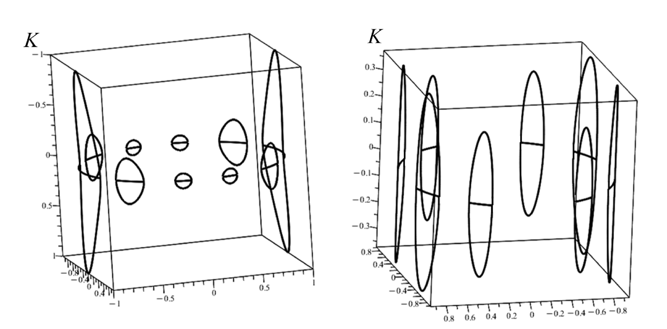
(a)                 (b)

Figure 3. ${\mathcal{A}}_{X}\cup Z_{\mathbb{R}}\subset{\mathbb{C}}\times{\mathbb{R}}$ for the odd $g$ (a) and the even $g$ (b).

Then we obviously have the following lemmas:

Lemma 3.6.

For $({\mathrm{e}}^{{\sqrt{-1}}\varphi_{j}},K_{j})_{j=1,2,\ldots,g}\in S^{g}Z$, the following holds:

$$\left[\begin{matrix}du_{1}\\ du_{2}\\ \vdots\\ du_{\ell}\\ \vdots\\ du_{g}\end{matrix}\right]=-\left[\frac{{\mathrm{e}}^{-(g-\ell){\sqrt{-1}}\varphi_{k}}(2{\sqrt{-1}}\sin\varphi_{k})^{\ell-1}}{(2{\sqrt{-1}})^{g-1}K_{k}}\right]\left[\begin{matrix}d\varphi_{1}\\ d\varphi_{2}\\ \vdots\\ d\varphi_{k}\\ \vdots\\ d\varphi_{g}\end{matrix}\right].$$

Let the matrix be denoted by ${\mathcal{L}}=({\mathcal{L}}_{ij})$, ${\mathcal{L}}_{ij}=\displaystyle{\left[\frac{(\cos\varphi_{j}-{\sqrt{-1}}\sin\varphi_{j})^{(g-i)}(2{\sqrt{-1}}\sin\varphi_{j})^{i-1}}{(2{\sqrt{-1}})^{g-1}K_{j}}\right]_{ij}}$. Then the determinant of ${\mathcal{L}}$,

$$\det({\mathcal{L}})=\displaystyle{\frac{\prod_{i<j}\sin(\varphi_{i}-\varphi_{j})}{(2{\sqrt{-1}})^{g(g-1)/2}K_{1}K_{2}\cdots K_{g}}}.$$

As in Appendix, by letting ${\mathfrak{s}}_{i}:={\sqrt{-1}}\sin\varphi_{i}$ and ${\mathfrak{c}}_{i}:=\cos\varphi_{i}$, we have

$${\mathcal{L}}_{ij}=\displaystyle{\left[\frac{({\mathfrak{c}}_{j}-{\mathfrak{s}}_{j})^{g-i}(2{\mathfrak{s}}_{j})^{i-1}}{(2{\sqrt{-1}})^{g-1}K_{j}}\right]}.$$

We also have the inverse of Lemma 3.6 at a regular locus, and let $\displaystyle{\prod_{i=1,\neq j}^{g}({\mathrm{e}}^{-{\sqrt{-1}}\varphi_{i}}\zeta-2{\sqrt{-1}}\sin(\varphi_{i}))}$ $=\varepsilon_{j,g-1}\zeta^{g-1}+\varepsilon_{j,g-2}\zeta^{g-2}+\cdots+\varepsilon_{j,1}\zeta+\varepsilon_{j,0}$. Then we obviously have $\varepsilon_{j,0}=\displaystyle{\prod_{i=1,\neq j}^{g}(-2{\sqrt{-1}}\sin(\varphi_{i}))}$. We introduce matrices

$${\mathcal{M}}:=\left[\varepsilon_{i,j-1}\right]=\left[\begin{matrix}\varepsilon_{1,0}&\varepsilon_{1,1}&\cdots&\varepsilon_{1,g-1}\\ \varepsilon_{2,0}&\varepsilon_{2,1}&\cdots&\varepsilon_{2,g-1}\\ \vdots&\vdots&\ddots&\vdots\\ \varepsilon_{g,0}&\varepsilon_{g,1}&\cdots&\varepsilon_{g,g-1}\end{matrix}\right],$$

$${\mathcal{K}}:=\left[\begin{matrix}\frac{[(2{\sqrt{-1}})^{-(g-1)(g-2)/2}K_{1}}{\prod_{i\neq 1}\sin(\varphi_{i}-\varphi_{1})}&&&\\ &\frac{(2{\sqrt{-1}})^{-(g-1)(g-2)/2}K_{2}}{\prod_{i\neq 2}\sin(\varphi_{i}-\varphi_{2})}&&\\ &&\ddots&\\ &&&\frac{(2{\sqrt{-1}})^{-(g-1)(g-2)/2}K_{1}}{\prod_{i\neq g}\sin(\varphi_{i}-\varphi_{g})}\end{matrix}\right].$$

For $g=3$ case, we have

$${\mathcal{M}}=-\begin{pmatrix}4\sin\varphi_{2}\sin\varphi_{3}&-2{\sqrt{-1}}(2{\sqrt{-1}}\sin\varphi_{2}\sin\varphi_{3}-\sin(\varphi_{2}+\varphi_{3}))&-{\mathrm{e}}^{-{\sqrt{-1}}(\varphi_{2}+\varphi_{3})}\\ 4\sin\varphi_{1}\sin\varphi_{3}&-2{\sqrt{-1}}(2{\sqrt{-1}}\sin\varphi_{1}\sin\varphi_{3}-\sin(\varphi_{3}+\varphi_{1}))&-{\mathrm{e}}^{-{\sqrt{-1}}(\varphi_{1}+\varphi_{3})}\\ 4\sin\varphi_{1}\sin\varphi_{2}&-2{\sqrt{-1}}(2{\sqrt{-1}}\sin\varphi_{1}\sin\varphi_{2}-\sin(\varphi_{1}+\varphi_{2}))&-{\mathrm{e}}^{-{\sqrt{-1}}(\varphi_{1}+\varphi_{2})}\\ \end{pmatrix}.$$

Lemma 3.7.

For $\varphi_{a}\in[\varphi_{\mathfrak{b}}^{[a-]},\varphi_{\mathfrak{b}}^{[a+]}]$, $(a=1,2,\ldots,g)$ such that $\varphi_{a}\neq\varphi_{b}$ $(a\neq b)$, we have

$${\begin{pmatrix}d\varphi_{1}\\ d\varphi_{2}\\ \vdots\\ d\varphi_{g}\end{pmatrix}={\mathcal{K}}{\mathcal{M}}\begin{pmatrix}du_{1}\\ du_{2}\\ \vdots\\ du_{g}\end{pmatrix}},\qquad{\mathcal{L}}^{-1}={\mathcal{K}}{\mathcal{M}}.$$ (3.7)

Proof.

The straightforward computations show it for $(\varphi_{\mathfrak{b}}^{[a-]},\varphi_{\mathfrak{b}}^{[a+]})$. Even at the branch point, this expression works since $\nu_{i}$ is a holomorphic one-form.   

We remark that (3.7) in Lemma 3.7 means that even if $\varphi_{j}$, $(j=1,2,\ldots,g)$ is real, $d\varphi_{j}$ is complex valued one-form. We let it decomposed to $d\varphi_{j}=d\varphi_{j,{\mathrm{r}}}+{\sqrt{-1}}d\varphi_{j,{\mathrm{i}}}$, $(j=1,2,\ldots,g)$. Further, we introduce $\varphi:=\varphi_{1}+\cdots+\varphi_{g}\in{\mathbb{R}}$ and $d\varphi=d\varphi_{{\mathrm{r}}}+{\sqrt{-1}}d\varphi_{{\mathrm{i}}}$; $\psi_{\mathrm{r}}=2\varphi$, $d\psi_{\mathrm{r}}=2d\varphi_{\mathrm{r}}$ and $d\psi_{\mathrm{i}}=2d\varphi_{\mathrm{i}}$ for $\psi$ in (2.5) and (2.6). We sometimes write $\varphi_{a,{\mathrm{r}}}:=\varphi_{a}$.

Remark 3.8.

For a point $\gamma^{\prime}\in{\widetilde{X}}$, the holomorphic one form $\nu(\gamma^{\prime})$ is regarded as $\nu(\gamma^{\prime})=\nu({\widehat{\kappa}}_{X}\gamma^{\prime})$. Lemma 3.6 means that for $u={\widetilde{v}}(\gamma=(\gamma_{1},\gamma_{2},\ldots,\gamma_{g}))=\displaystyle{\sum\int_{\gamma_{i}}\nu}$, $du=d{\widetilde{v}}(\gamma)$ is equal to $\sum\nu(\gamma_{i})$.

We regard this as a linear transformation of $d\gamma_{i}$, i.e.,

$$du={\mathcal{L}}\displaystyle{\begin{pmatrix}d\varphi_{1}(\gamma_{1})\\ \vdots\\ d\varphi_{g}(\gamma_{g})\end{pmatrix}}.$$

The matrix ${\mathcal{L}}$ is the matrix representation of the linear transformation ${\mathcal{L}}$ $:T^{*}S^{g}{\widetilde{Z}}\to T^{*}_{u}{\mathbb{C}}^{g}$. Since ${\mathcal{L}}$ is invertible due to the Abel-Jacobi theorem for the regular locus, we have

$${\begin{pmatrix}d\varphi_{1}\\ \vdots\\ d\varphi_{g}\end{pmatrix}}={\mathcal{L}}^{-1}\displaystyle{\begin{pmatrix}du_{1}\\ \vdots\\ du_{g}\end{pmatrix}}={\mathcal{K}}{\mathcal{M}}\displaystyle{\begin{pmatrix}du_{1}\\ \vdots\\ du_{g}\end{pmatrix}}.$$

Then the transformation ${\mathcal{L}}^{-1}$ (or the matrix ${\mathcal{K}}{\mathcal{M}}$) can be also interpreted as the pullback ${\widetilde{v}}^{*}:T^{*}_{u}{\widetilde{v}}(S^{g}{\widetilde{Z}})\to T^{*}_{\gamma}S^{g}{\widetilde{X}}$ for points ${\widetilde{v}}(\gamma)=u\in{\mathbb{C}}^{g}$ and $\gamma\in S^{g}{\widetilde{Z}}$.

Assumption 3.9.

For simplicity, in this paper, we restrict $S^{g}{\widetilde{Z}}_{\mathbb{R}}\subset S^{g}{\widetilde{X}}$ to $[S^{g}{\widetilde{Z}}_{\mathbb{R}}]^{0}:=$ $\kappa_{\widehat{X}}^{-1}\prod_{a=1}^{g}[\varphi_{\mathfrak{b}}^{[a-]},\varphi_{\mathfrak{b}}^{[a+]}]$, where $\prod_{a=1}^{g}[\varphi_{\mathfrak{b}}^{[a-]},\varphi_{\mathfrak{b}}^{[a+]}]\subset S^{g}{\mathcal{A}}_{X}^{\varphi}$. In other words, for $(\gamma_{1},\ldots,\gamma_{g})\in S^{g}{\widetilde{Z}}_{\mathbb{R}}$, we can set $\gamma_{i}$ into $[\varphi_{\mathfrak{b}}^{[i-]},\varphi_{\mathfrak{b}}^{[i+]}]$ respectively so that we can avoid the intersection between $\gamma_{i}$ and $\gamma_{j}$ for $i\neq j$.

Remark 3.10.

We consider the transformation ${\mathcal{L}}^{-1}$ (or the matrix ${\mathcal{K}}{\mathcal{M}}$) as the pullback ${\widetilde{v}}^{*}:T^{*}_{u}{\widetilde{v}}([S^{g}{\widetilde{Z}}_{\mathbb{R}}]^{0})\to T^{*}_{\gamma}S^{g}{\widetilde{X}}$ for points ${\widetilde{v}}(\gamma)=u\in{\mathbb{C}}^{g}$ and $\gamma\in[S^{g}{\widetilde{Z}}_{\mathbb{R}}]^{0}$ in this paper..

We should note that Weierstrass basically considered these maps to find his sigma function, Al-function in [26] by implicitly studying the sine-Gordon equation, and Baker also essentially used this matrix to find the so-called KdV hierarchy in [3]. They expressed $\partial_{u_{i}}$ in terms of $\partial_{x_{i}}$ by using such a matrix, and realized the inversion problem of ${\widetilde{v}}$ or $v$ as the Jacobi inversion formula.

4. Real hyperelliptic solutions of the gauged MKdV equation over ${\mathbb{R}}$

We will go on to assume $[S^{g}{\widetilde{Z}}_{\mathbb{R}}]^{0}$ as the non-singular locus of ${\widetilde{v}}^{*}$ and ${\widetilde{v}}^{-1*}$. As we show its proof and background in Appendix, this angle expression provides the following lemma, which is the key lemma in this paper:

Lemma 4.1.

We define a $g\times g$ matrix:

For the odd $g$ case, let

$${\mathcal{V}}:=\left[\begin{matrix}\mathfrak{Re}\varepsilon_{1,0}&\mathfrak{Im}\varepsilon_{1,2}&\cdots&\mathfrak{Im}\varepsilon_{1,2\ell}&\mathfrak{Re}\varepsilon_{1,2\ell}&\cdots&\mathfrak{Im}\varepsilon_{1,g-1}&\mathfrak{Re}\varepsilon_{1,g-1}\\ \mathfrak{Re}\varepsilon_{2,0}&\mathfrak{Im}\varepsilon_{2,2}&\cdots&\mathfrak{Im}\varepsilon_{2,2\ell}&\mathfrak{Re}\varepsilon_{2,2\ell}&\cdots&\mathfrak{Im}\varepsilon_{2,g-1}&\mathfrak{Re}\varepsilon_{2,g-1}\\ \vdots&\vdots&\ddots&\vdots&\vdots&\ddots&\vdots&\vdots&\\ \mathfrak{Re}\varepsilon_{g-1,0}&\mathfrak{Im}\varepsilon_{g-1,2}&\cdots&\mathfrak{Im}\varepsilon_{g-1,2\ell}&\mathfrak{Re}\varepsilon_{g-1,2\ell}&\cdots&\mathfrak{Im}\varepsilon_{g-1,g-1}&\mathfrak{Re}\varepsilon_{g-1,g-1}\\ \mathfrak{Re}\varepsilon_{g,0}&\mathfrak{Im}\varepsilon_{g,2}&\cdots&\mathfrak{Im}\varepsilon_{g,2\ell}&\mathfrak{Re}\varepsilon_{g-1,2\ell}&\cdots&\mathfrak{Im}\varepsilon_{g,g-1}&\mathfrak{Re}\varepsilon_{g,g-1}\end{matrix}\right].$$

For the even $g$ case, let

$${\mathcal{V}}:=\left[\begin{matrix}\mathfrak{Im}\varepsilon_{1,1}&\mathfrak{Re}\varepsilon_{1,1}&\cdots&\mathfrak{Im}\varepsilon_{1,2\ell-1}&\mathfrak{Re}\varepsilon_{1,2\ell-1}&\cdots&\mathfrak{Im}\varepsilon_{1,g-1}&\mathfrak{Re}\varepsilon_{1,g-1}\\ \mathfrak{Im}\varepsilon_{2,1}&\mathfrak{Re}\varepsilon_{2,1}&\cdots&\mathfrak{Im}\varepsilon_{2,2\ell-1}&\mathfrak{Re}\varepsilon_{2,2\ell-1}&\cdots&\mathfrak{Im}\varepsilon_{2,g-1}&\mathfrak{Re}\varepsilon_{2,g-1}\\ \vdots&\vdots&\ddots&\vdots&\vdots&\ddots&\vdots&\vdots&\\ \mathfrak{Im}\varepsilon_{g-1,1}&\mathfrak{Re}\varepsilon_{g-1,1}&\cdots&\mathfrak{Im}\varepsilon_{g-1,2\ell-1}&\mathfrak{Re}\varepsilon_{g-1,2\ell-1}&\cdots&\mathfrak{Im}\varepsilon_{g-1,g-1}&\mathfrak{Re}\varepsilon_{g-1,g-1}\\ \mathfrak{Im}\varepsilon_{g,1}&\mathfrak{Re}\varepsilon_{g-1,1}&\cdots&\mathfrak{Im}\varepsilon_{g,2\ell-1}&\mathfrak{Re}\varepsilon_{g,2\ell-1}&\cdots&\mathfrak{Im}\varepsilon_{g,g-1}&\mathfrak{Re}\varepsilon_{g,g-1}\\ \end{matrix}\right].$$

Then ${\mathcal{K}}{\mathcal{M}}$ is expressed as

$${\mathcal{K}}{\mathcal{M}}={\mathcal{V}}{\mathcal{B}},\qquad{\mathcal{B}}=\begin{pmatrix}{\mathcal{B}}^{[g-3,g-3]}&{\mathcal{B}}^{[g-3],1}&{\mathcal{B}}^{[g-3],2}&0\\ 0&1&-1&0\\ 0&0&-2{\sqrt{-1}}&{\sqrt{-1}}\\ 0&0&0&1\end{pmatrix}\in\mathrm{GL}({\mathbb{Q}}[{\sqrt{-1}}],g),$$

where ${\mathcal{B}}^{[g-3,g-3]}\in\mathrm{Mat}_{\mathbb{C}}((g-3)\times(g-3))$, ${\mathcal{B}}^{[g-3],1},{\mathcal{B}}^{[g-3],2}\in\mathrm{Mat}_{\mathbb{C}}((g-3)\times 1)$, and $0$ denotes a zero $\ell\times k$ matrix, although $(0)=0$. Further, ${\mathcal{B}}^{[g-3],2}={\,{}^{t}\negthinspace}({\mathfrak{b}}_{1},{\sqrt{-1}}{\mathfrak{b}}_{2},\ldots,{\mathfrak{b}}_{g-4},{\sqrt{-1}}{\mathfrak{b}}_{g-3})$ for an odd $g$ and ${\mathcal{B}}^{[g-3],2}={\,{}^{t}\negthinspace}({\sqrt{-1}}{\mathfrak{b}}_{1},{\mathfrak{b}}_{2},\ldots,{\mathfrak{b}}_{g-4},{\sqrt{-1}}{\mathfrak{b}}_{g-3})$ for an even $g$.

Proof.

See Appendix, i.e., Corollary A.9.  

In other words, we will decompose the image of the Abelian integral or the Abel-Jacobi map from a real analytic viewpoint or consider the linear transformation in $T^{*}{\mathbb{C}}^{g}$ to $T^{*}{\mathbb{C}}^{g}$:

$$\begin{pmatrix}du_{1}\\ \vdots\\ du_{g}\end{pmatrix}={\mathcal{B}}^{-1}\begin{pmatrix}dt_{1}\\ \vdots\\ dt_{g}\end{pmatrix},\quad\begin{pmatrix}dt_{1}\\ \vdots\\ dt_{g}\end{pmatrix}={\mathcal{B}}\begin{pmatrix}du_{1}\\ \vdots\\ du_{g}\end{pmatrix}.$$ (4.1)

We let the former matrix denoted by ${\mathcal{D}}$, and also define $dt:=dt_{g-2}$ and $ds:=dt_{g}$.

Lemma 4.2.

Let the basis $\displaystyle{\left\{{\mathcal{B}}^{-1}=[{\mathbf{e}}_{1},{\mathbf{e}}_{2},\ldots,{\mathbf{e}}_{g}]\right\}}$ of ${\mathbb{C}}^{g}$, i.e.,

$${\mathbb{C}}^{g}=\langle{\mathbf{e}}_{1},{\mathbf{e}}_{2},\ldots,{\mathbf{e}}_{g}\rangle_{\mathbb{C}},\quad{\mathbb{R}}^{2}=\langle{\mathbf{e}}_{g-1},{\mathbf{e}}_{g}\rangle_{\mathbb{R}}\subset{\mathbb{C}}^{g}.$$ (4.2)

Then we have

$$({\mathbf{e}}_{1},{\mathbf{e}}_{2},\ldots,{\mathbf{e}}_{g})={\mathcal{L}}({\mathcal{V}}_{1},{\mathcal{V}}_{2},\ldots,{\mathcal{V}}_{g}).$$

Since (4.1) also shows

$$({\mathcal{V}}_{1},{\mathcal{V}}_{2},\ldots,{\mathcal{V}}_{g})=\begin{pmatrix}\partial_{t_{1}}\varphi_{1}&\partial_{t_{2}}\varphi_{1}&\cdots&\partial_{t_{g}}\varphi_{1}\\ \partial_{t_{1}}\varphi_{2}&\partial_{t_{2}}\varphi_{2}&\cdots&\partial_{t_{g}}\varphi_{2}\\ \vdots&\vdots&\ddots&\vdots\\ \partial_{t_{1}}\varphi_{g}&\partial_{t_{2}}\varphi_{g}&\cdots&\partial_{t_{g}}\varphi_{g}\end{pmatrix},\quad\begin{pmatrix}d\varphi_{1}\\ d\varphi_{2}\\ \vdots\\ d\varphi_{g}\end{pmatrix}=({\mathcal{V}}_{1},{\mathcal{V}}_{2},\ldots,{\mathcal{V}}_{g})\begin{pmatrix}dt_{1}\\ dt_{2}\\ \vdots\\ dt_{g}\end{pmatrix},$$

the relations between differential operators are given by

$$\begin{pmatrix}\partial_{t_{1}}\\ \partial_{t_{2}}\\ \vdots\\ \partial_{t_{g}}\end{pmatrix}={\,{}^{t}\negthinspace}{\mathcal{B}}^{-1}\begin{pmatrix}\partial_{u_{1}}\\ \partial_{u_{2}}\\ \vdots\\ \partial_{u_{g}}\end{pmatrix},\quad\begin{pmatrix}\partial_{u_{1}}\\ \partial_{u_{2}}\\ \vdots\\ \partial_{u_{g}}\end{pmatrix}={\,{}^{t}\negthinspace}{\mathcal{B}}\begin{pmatrix}\partial_{t_{1}}\\ \partial_{t_{2}}\\ \vdots\\ \partial_{t_{g}}\end{pmatrix},{\,{}^{t}\negthinspace}{\mathcal{B}}=\begin{pmatrix}{\,{}^{t}\negthinspace}{\mathcal{B}}^{[g-3,g-3]}&0&0&0\\ {\,{}^{t}\negthinspace}{\mathcal{B}}^{[g-3],1}&1&0&0\\ {\,{}^{t}\negthinspace}{\mathcal{B}}^{[g-3],2}&-1&-2{\sqrt{-1}}&0\\ 0&0&{\sqrt{-1}}&1\end{pmatrix}.$$ (4.3)

Thus we have the relations,

$$\partial_{u_{g}}=\partial_{t_{g}}+{\sqrt{-1}}\partial_{t_{g-1}},\quad\partial_{u_{g-1}}=-\partial_{t_{g-2}}-2{\sqrt{-1}}\partial_{t_{g-1}}+\sum_{j=1}^{g-3}\sqrt{(-1)^{j}}{\mathfrak{b}}_{g-2-j}\partial_{t_{g-2-j}}.$$ (4.4)

Using them, we have the following lemma:

Lemma 4.3.

$$\partial_{t_{a}}\psi=(1,1,\ldots,1,1){\mathcal{V}}_{a}={\mathcal{V}}_{a,1}+{\mathcal{V}}_{a,2}+\cdots+{\mathcal{V}}_{a,g},\quad(a=1,2,\ldots,g),$$

$$\partial_{u_{g-1}}\psi=(1,1,\ldots,1,1)({\mathcal{V}}_{g-2}+2{\sqrt{-1}}{\mathcal{V}}_{g-1}+\sum_{j=1}^{g-3}\sqrt{(-1)^{j}}{\mathfrak{b}}_{g-2-j}{\mathcal{V}}_{g-2-j}),$$

$$\partial_{u_{g}}\psi=(1,1,\ldots,1,1)({\mathcal{V}}_{g}+{\sqrt{-1}}{\mathcal{V}}_{g-1}).$$

Here we recall the Cauchy-Riemann relations of these parameters:

Proposition 4.4.

Recall $u_{a}=u_{a{\mathrm{r}}}+{\sqrt{-1}}u_{a{\mathrm{i}}}$ and let $t_{a}:=t_{a{\mathrm{r}}}+{\sqrt{-1}}t_{a{\mathrm{i}}}$ for $a=1,2,\ldots,g$. For a complex analytic function $\psi=\psi_{\mathrm{r}}+{\sqrt{-1}}\psi_{\mathrm{i}}$, (4.3) shows

$$\partial_{u_{a}{\mathrm{r}}}\psi_{\mathrm{r}}=\partial_{u_{a}{\mathrm{i}}}\psi_{\mathrm{i}},\qquad\partial_{u_{a}{\mathrm{r}}}\psi_{\mathrm{i}}=-\partial_{u_{a}{\mathrm{i}}}\psi_{\mathrm{r}}.\qquad(a=1,2,\ldots,g),$$

$$\partial_{t_{a}{\mathrm{r}}}\psi_{\mathrm{r}}=\partial_{t_{a}{\mathrm{i}}}\psi_{\mathrm{i}},\qquad\partial_{t_{a}{\mathrm{r}}}\psi_{\mathrm{i}}=-\partial_{t_{a}{\mathrm{i}}}\psi_{\mathrm{r}}.\qquad(a=1,2,\ldots,g).$$

Proof.

Since the Cauchy-Riemann relations are given by $\overline{\partial_{u_{a}}}\psi=\overline{\partial_{t_{a}}}\psi=0$, we obtain them.  

Since we are concerned with the case that $\varphi_{a}\in{\mathbb{R}}$, i.e., $\varphi_{a,{\mathrm{i}}}=0$, $(a=1,2,\ldots,g)$, we may assume that $t_{a}\in{\mathbb{R}}$ belongs to ${\mathbb{C}}^{g}$. Equation (4.4), Lemma 4.3 and Proposition 4.4 show the following lemma:

Lemma 4.5.

For $\varphi_{a}\in{\mathbb{R}}$, i.e., $\varphi_{a,{\mathrm{i}}}=0$, $(a=1,2,\ldots,g)$, the following relations hold:

1. $\partial_{u_{g-1}}\psi=\partial_{u_{g-1},{\mathrm{r}}}\psi_{\mathrm{r}}-{\sqrt{-1}}\partial_{u_{g-1},{\mathrm{i}}}\psi_{\mathrm{r}}=\partial_{u_{g-1},{\mathrm{r}}}\psi_{\mathrm{r}}+{\sqrt{-1}}\partial_{u_{g-1},{\mathrm{r}}}\psi_{\mathrm{i}}=-\partial_{t_{g-2},{\mathrm{r}}}\psi_{\mathrm{r}}-2{\sqrt{-1}}\partial_{t_{g-1},{\mathrm{r}}}\psi_{\mathrm{r}}$ $\displaystyle{+\sum_{j=1}^{g-3}\sqrt{(-1)^{j}}{\mathfrak{b}}_{g-2-j}\partial_{t_{g-2-j}}\psi_{\mathrm{r}}}$. $=(1,\ldots,1)(-{\mathcal{V}}_{g-1}-2{\sqrt{-1}}{\mathcal{V}}_{g-1}$ $\displaystyle{+\sum_{j=1}^{g-3}\sqrt{(-1)^{j}}{\mathfrak{b}}_{g-2-j}{\mathcal{V}}_{g-2-j})}$.

2. $\partial_{u_{g}}\psi=\partial_{u_{g},{\mathrm{r}}}\psi_{\mathrm{r}}-{\sqrt{-1}}\partial_{u_{g},{\mathrm{i}}}\psi_{\mathrm{r}}=\partial_{u_{g},{\mathrm{r}}}\psi_{\mathrm{r}}+{\sqrt{-1}}\partial_{u_{g},{\mathrm{r}}}\psi_{\mathrm{i}}=\partial_{t_{g},{\mathrm{r}}}\psi_{\mathrm{r}}+{\sqrt{-1}}\partial_{t_{g-1},{\mathrm{r}}}\psi_{\mathrm{r}}$ $=(1,\ldots,1)({\mathcal{V}}_{g}+{\sqrt{-1}}{\mathcal{V}}_{g-1})$.

3. Particularly we have

   $$\partial_{u_{g-1},{\mathrm{r}}}\psi_{\mathrm{r}}=(-\partial_{t_{g-2},{\mathrm{r}}}+\sum_{j=1}^{\lfloor(g-3)/2\rfloor}{\mathfrak{b}}_{g-2-2j}\partial_{t_{g-2-2j}})\psi_{\mathrm{r}}$$

   $$=(1,\ldots,1)(-{\mathcal{V}}_{g-2}+\sum_{j=1}^{\lfloor(g-3)/2\rfloor}{\mathfrak{b}}_{g-2-2j}{\mathcal{V}}_{g-2-2j})$$

   $$\partial_{u_{g-1},{\mathrm{r}}}\psi_{\mathrm{i}}=(2\partial_{t_{g-1},{\mathrm{r}}},+\sum_{j=1}^{\lfloor(g-3)/2\rfloor}{\mathfrak{b}}_{g-1-2j}\partial_{t_{g-1-2j}})\psi_{\mathrm{i}}$$

   $$=(1,\ldots,1)({\mathcal{V}}_{g-1}+\sum_{j=1}^{\lfloor(g-3)/2\rfloor}{\mathfrak{b}}_{g-1-2j}{\mathcal{V}}_{g-1-2j},$$

   $$\partial_{u_{g},{\mathrm{r}}}\psi_{\mathrm{r}}=\partial_{t_{g},{\mathrm{r}}}\psi_{\mathrm{r}}=(1,\ldots,1){\mathcal{V}}_{g},\quad\partial_{u_{g},{\mathrm{i}}}\psi_{\mathrm{r}}=-\partial_{t_{g-1},{\mathrm{r}}}\psi_{\mathrm{r}}=-(1,\ldots,1){\mathcal{V}}_{g-1}.$$ (4.5)

Proof.

We obviously obtain them.  

Remark 4.6.

Lemma 4.5 does not claim that there is a different complex structure in $J_{X}$ and the image of ${\widetilde{v}}$. These parameterizations are consistent only for the local regions related to the arcs of $S^{1}$ in ${\widehat{\kappa}}_{X}{\widehat{X}}$, or $\varphi_{a}\in{\mathbb{R}}$ and $\varphi_{a,{\mathrm{i}}}=0$ ($a=1,2,\ldots,g$). This means that we simply embed the real vector space ${\mathbb{R}}^{g}$ in ${\mathbb{C}}^{g}$ via the matrix ${\mathcal{B}}$ and ${\mathcal{B}}^{-1}$.

The FGMKdV equations (2.6) with Lemma 4.5 can be expressed in terms of the parameterizations of $t$s. Since these $dt_{a}$ are linearly independent, we can set $dt_{i}=0$ $i<g-2$. We give the first theorem in this paper.

Theorem 4.7.

Assume $\varphi_{i}\in{\mathbb{R}}$, $(i=1,2,\ldots,g)$, i.e., $\psi\in{\mathbb{R}}$ or $\psi_{{\mathrm{i}}}=0$. Let $t:=t_{g-2{\mathrm{r}}}$, ${\mathfrak{t}}:=t_{g-1{\mathrm{i}}}$, and $s:=t_{g{\mathrm{r}}}$ belonging to ${\mathbb{R}}$, and let us consider

$$\begin{pmatrix}d\varphi_{1}\\ d\varphi_{2}\\ \vdots\\ d\varphi_{g}\end{pmatrix}=({\mathcal{V}}_{g-2},{\sqrt{-1}}{\mathcal{V}}_{g-1},{\mathcal{V}}_{g})\begin{pmatrix}dt\\ d{\mathfrak{t}}\\ ds\end{pmatrix}.$$ (4.6)

Then (2.5) is reduced to the coupled FGMKdV equations,

$$(\partial_{u_{g-1},{\mathrm{r}}}-\frac{1}{2}(\lambda_{6}+3b_{0}+\frac{3}{4}(\partial_{\mathfrak{t}}\psi_{\mathrm{r}})^{2})\partial_{s})\psi_{\mathrm{r}}+\frac{1}{8}\left(\partial_{s}\psi_{\mathrm{r}}\right)^{3}+\frac{1}{4}\partial_{s}^{3}\psi_{\mathrm{r}} = 0,$$ (4.7)

$$(\partial_{u_{g-1},{\mathrm{i}}}-\frac{1}{2}(\lambda_{6}+3b_{0}-\frac{3}{4}(\partial_{s}\psi_{\mathrm{r}})^{2})\partial_{{\mathfrak{t}}})\psi_{\mathrm{r}}+\frac{1}{8}\left(\partial_{{\mathfrak{t}}}\psi_{\mathrm{r}}\right)^{3}+\frac{1}{4}\partial_{{\mathfrak{t}}}^{3}\psi_{\mathrm{r}} = 0.$$ (4.8)

If $\partial_{s}\psi_{\mathrm{i}}=\partial_{\mathfrak{t}}\psi_{\mathrm{r}}=0$ for a region, (4.7) is further reduced to the focusing MKdV equation over ${\mathbb{R}}$. Note that $\partial_{\mathfrak{t}}\psi_{{\mathrm{i}}}=\partial_{u_{g},{\mathrm{r}}}\psi_{{\mathrm{i}}}$.

We recall that ${\widetilde{\gamma}}_{i}$ of $(\gamma_{1},\ldots,\gamma_{g})\in[S^{g}{\widetilde{Z}}_{\mathbb{R}}]^{0}$ forms a loop illustrated in Figure 3.

Theorem 4.7 leads to the nice property that the conditions CI and CII in Condition 2.4 are satisfied. We explicitly describe the property following [17].

Theorem 4.8.

Let $(P_{a,0}=({\mathrm{e}}^{{\sqrt{-1}}\varphi_{a,0}},$ $K_{a,0})_{a=1,\ldots,g}$ be a point in $\kappa_{\widehat{X}}[S^{g}{\widetilde{Z}}_{\mathbb{R}}]^{0}$ where $\varphi_{a,0}\in[\varphi_{\mathfrak{b}}^{[a-]},\varphi_{\mathfrak{b}}^{[a+]}]$, and set $\gamma_{0}\in S^{g}{\widetilde{X}}$ such that $\kappa_{X}\gamma_{0}=(P_{1,0},P_{2,0},\ldots,P_{g,0})$. For $(t,s)\in{\mathbb{R}}^{2}$,

$$\begin{pmatrix}\varphi_{1}(t,s)\\ \varphi_{2}(t,s)\\ \vdots\\ \varphi_{g}(t,s)\end{pmatrix}:=\left(\int^{t}_{0}{\mathcal{V}}_{1}dt+\int^{s}_{0}{\mathcal{V}}_{g}ds\right)+\begin{pmatrix}\varphi_{1,0}\\ \varphi_{2,0}\\ \vdots\\ \varphi_{g,0}\end{pmatrix}$$ (4.9)

forms $\gamma(t,s)\in S^{g}{\widetilde{Z}}_{\mathbb{R}}\subset S^{g}{\widetilde{X}}$ i.e., $\gamma:{\mathbb{R}}^{2}\to S^{g}{\widetilde{X}}$, by setting $K_{i}>0$ for $d\varphi_{i}>0$ and $K_{i}\leq 0$ otherwise. Then the image of $\gamma$,

$${{\widetilde{\mathbb{S}}}}_{\gamma_{0}}:=\{\gamma(t,s)\ |\ (t,s)\in{\mathbb{R}}^{2}\}\subset S^{g}{\widetilde{Z}}_{\mathbb{R}},$$ (4.10)

provides a global solution of the FGMKdV equation in Theorem 4.7.

Proof.

Essentially the same as the proof in Proposition 5.4 in [17]. Note that $[\varphi_{\mathfrak{b}}^{[a-]},\varphi_{\mathfrak{b}}^{[a+]}]$ are disjoint, i.e., $[\varphi_{\mathfrak{b}}^{[a-]},\varphi_{\mathfrak{b}}^{[a+]}]\cap[\varphi_{\mathfrak{b}}^{[b-]},\varphi_{\mathfrak{b}}^{[b+]}]=\emptyset$ for $a\neq b$. Thus for a given $(\varphi_{a,0})\in[\varphi_{\mathfrak{b}}^{[a-]},\varphi_{\mathfrak{b}}^{[a+]}]$, $\gamma(t,s)$ belongs to $[S^{g}Z_{\mathbb{R}}]^{0}$ whose $i$-th component belongs to $\kappa_{Z}^{-1}[\varphi_{\mathfrak{b}}^{[a-]},\varphi_{\mathfrak{b}}^{[a+]}]$. Since the integrals are contours integrals on the disjoint loops in $S^{g}Z_{\mathbb{R}}$ and thus there is no intersection, we can simply integrate the orbits and find $\gamma\in S^{g}{\widetilde{Z}}_{\mathbb{R}}$ for every $(t,s)\in{\mathbb{R}}^{2}$.  

Remark 4.9.

In this paper we restrict ourselves to $[S^{g}{\widetilde{Z}}_{\mathbb{R}}]^{0}$. However, there are other possibilities; we can directly extend our arguments for the cases $S^{g}{\widetilde{Z}}_{{\sqrt{-1}}{\mathbb{R}}}$ which correspond to $u_{a,{\mathrm{i}}}$ as in (2.6). Furthermore, we avoid the intersection of the paths $\gamma_{i}$ and $\gamma_{j}$, $(i\neq j)$, but we could consider the intersection as argued in the previous paper [17]. Moreover, there are further possibilities as the real hyperelliptic solutions of the FGMKdV equations; for example, some of $e_{j}$ and $e_{j+1}=1/e_{j}$ can be real.

Remark 4.10.

Here we give some comments on condition III $\partial_{u_{g},{\mathrm{r}}}\psi=$ constant. The condition is now given by $(1,1,\ldots,1){\mathcal{V}}_{g-1}=$ constant. This is realized as the vanishing of the meromorphic functions on $S^{g}{\widehat{X}}$ and thus on ${\widehat{J}}_{X}$. It might be obtained by the ratio of the sigma functions. Thus, it should be written down more concretely and studied from an algebraic geometric point of view in the future.

Remark 4.11.

In our investigation, we have considered the differential relations given by the symmetric functions on $S^{g}{\widehat{X}}$. There we deal with the derivatives of the quotient ring ${\mathbb{C}}[{\mathfrak{c}}_{1},{\mathfrak{s}}_{1},K_{1},\ldots,{\mathfrak{c}}_{g},{\mathfrak{s}}_{g},K_{g}]$ divided by ${\mathfrak{c}}_{i}^{2}-{\mathfrak{s}}_{i}^{2}=1$, and (3.4). Recently, Buchstaber and Mikhailov investigated such systems as the Lie algebras of vector fields on universal bundles of symmetric product of curves, and as an integrable Hamiltonian system there [5, 6]. These visions give a sophisticated interpretation from a modern mathematical point of view of the methods of Weierstrass [26] and Baker [3] on which we are based. If so, the rewrite may reveal the mathematical essence of our approach and provide a foundation between biophysics and modern mathematics, since this system is closely related to the shapes of supercoiled DNA via the excited states of Euler’s elastica.

5. Discussion and Conclusion

By extending the constructions in [17, 20], in this paper, we showed a novel real algebro-geometric method to obtain the hyperelliptic solutions of general genera $g$ of the FGMKdV equation (2.6) as in Theorems 4.7 and 4.8. As we introduced the real parameters $t$ in the Jacobian $J_{X}$ in (4.1), we showed that these new parameters $t_{g}$ and $t_{g-2}$ provide the correspondence between the real data in $J_{X}$ and real $\varphi$’s in $S^{g}{\widehat{X}}$. Since the FGMKdV equation (2.6) is a differential identity on $S^{g}{\widehat{X}}$, the correspondence means the construction of the real hyperelliptic solutions of the FGMKdV equation. In the correspondence, the shifted elementary symmetric polynomial plays the essential role, since even on the angle expression, the correspondence basically comes from the properties of the Vandermonde matrices. (We describe the properties of the shifted elementary symmetric polynomials in Appendix.)

In the construction we have used the data of the hyperelliptic curves $X$ directly instead of the Jacobian $J_{X}$. We note that our algebraic study of the algebraic curves on two decades [4, 24, 21] based on studies by Weierstrass [26] and Baker [3] allows the such treatment.

The ultimate purpose of this study is to find the real solution of the focusing MKdV equation of higher genus explicitly for the fascinating relation between shapes of supercoiled DNA and the integrable system as mentioned in Introduction and in [18]. Since the condition of the gauge field $\partial_{s}\psi_{{\mathrm{i}}}$ requires more higher genus, our results may step to reveal the properties of the conditions as mentioned in Remark 4.10; our approach could be rewritten in the framework of the modern investigation by Buchstaber and Mikhailov [5, 6] as in Remark 4.11, and then the rewrite might have a new insight into the condition.

Although we studied the case of $[S^{g}{\widetilde{Z}}_{\mathbb{R}}]^{0}$ of $S^{g}{\widetilde{Z}}_{\mathbb{R}}$ and the branch points $(b_{i},0)$ in $S^{1}$, there are many other configurations of $\gamma_{i}$ and branch points that generate real $K$ as in [16] as mentioned in Remark 4.9. In the future we should classify the moduli of the hyperelliptic solutions of the FGMKdV equation of genus $g$.

Furthermore, when we extend the statistical mechanics of plane curves to that of space curves, we require the similar construction of the hyperelliptic solutions of the nonlinear Schrödinger equation of genus $g$, although we partially obtained them in [19]. The results in this paper will have strong implications for such a generalization.

A. Appendix

Lemmas 3.7, 4.1 and 4.5 are key lemmas in this paper but their proofs are very complicated. In this appendix, we show their background and proofs. Here, we consider the shifted elementary symmetry polynomials.

Let us consider the polynomial ring $R:={\mathbb{C}}[{\mathfrak{s}}_{1},\ldots,{\mathfrak{s}}_{n},{\mathfrak{c}}_{1},\ldots,{\mathfrak{c}}_{n}]$ and its permutation $\tau\in{\mathfrak{S}}_{n}$ on their indices, ${\mathbb{C}}[{\mathfrak{s}}_{\tau(1)},$ $\ldots,{\mathfrak{s}}_{\tau(n)},{\mathfrak{c}}_{\tau(1)},\ldots,{\mathfrak{c}}_{\tau(n)}]$. We have a symmetric ring $SR:=R/{\mathfrak{S}}_{n}$, and its homogeneous part $SR_{\ell}$ of degree $\ell$. Further, for its subring $R^{(j)}:={\mathbb{C}}[{\mathfrak{s}}_{1},\ldots,\check{{\mathfrak{s}}}_{j},\ldots,{\mathfrak{s}}_{n},{\mathfrak{c}}_{1},\ldots,\check{{\mathfrak{c}}}_{j},\ldots,{\mathfrak{c}}_{n}]$ and its permutation $\tau^{(j)}\in{\mathfrak{S}}_{n-1}$ on their indices ${\mathbb{C}}[{\mathfrak{s}}_{\tau^{(j)}(1)},$ $\ldots,\check{{\mathfrak{s}}}_{j},\ldots,{\mathfrak{s}}_{\tau^{(j)}(n)},{\mathfrak{c}}_{\tau^{(j)}(1)},\ldots,\check{{\mathfrak{c}}}_{j},\ldots,{\mathfrak{c}}_{\tau^{(j)}(n)}]$, we consider the symmetric ring $SR^{(j)}:=R^{(j)}/{\mathfrak{S}}_{n-1}$ whose elements are invariant by $\tau^{(j)}\in{\mathfrak{S}}_{n-1}$, and its homogeneous part $SR_{\ell}^{(j)}$ of degree $\ell$. Here check on top of a letter signifies deletion.

Let $\displaystyle{\prod_{i=1,\neq j}^{n}(({\mathfrak{c}}_{i}-{\mathfrak{s}}_{i})x-2{\mathfrak{s}}_{i})}$ $=\varepsilon_{j,n-1}x^{n-1}+\varepsilon_{j,n-2}x^{n-2}+\cdots+\varepsilon_{j,1}x+\varepsilon_{j,0}$. Then we obviously have the relations, $\varepsilon_{j,k}\in SR^{(j)}$, $\varepsilon_{j,0}=\displaystyle{\prod_{i=1,\neq j}^{n}2{\mathfrak{s}}_{i}}$, and $\varepsilon_{j,n-1}=\displaystyle{\prod_{i=1,\neq j}^{n}({\mathfrak{c}}_{i}-{\mathfrak{s}}_{i})}$.

We will show the following first proposition.

Proposition A.1.

For a matrix ${\mathcal{W}}\in\mathrm{Mat}_{R}(n)$ given by

$$\left[\begin{matrix}({\mathfrak{c}}_{1}-{\mathfrak{s}}_{1})^{n-1}&({\mathfrak{c}}_{2}-{\mathfrak{s}}_{2})^{n-1}&\cdots&({\mathfrak{c}}_{\ell}-{\mathfrak{s}}_{\ell})^{n-1}&\cdots&({\mathfrak{c}}_{n}-{\mathfrak{s}}_{n})^{n-1}\\ 2{\mathfrak{s}}_{1}({\mathfrak{c}}_{1}-{\mathfrak{s}}_{1})^{n-2}&2{\mathfrak{s}}_{2}({\mathfrak{c}}_{2}-{\mathfrak{s}}_{2})^{n-2}&\cdots&2{\mathfrak{s}}_{\ell}({\mathfrak{c}}_{\ell}-{\mathfrak{s}}_{\ell})^{n-2}&\cdots&2{\mathfrak{s}}_{n}({\mathfrak{c}}_{\ell}-{\mathfrak{s}}_{\ell})^{n-2}\\ \vdots&\vdots&\ddots&\vdots&\ddots&\vdots\\ (2{\mathfrak{s}}_{1})^{\ell}({\mathfrak{c}}_{1}-{\mathfrak{s}}_{1})^{n-\ell-1}&(2{\mathfrak{s}}_{2})^{\ell}({\mathfrak{c}}_{2}-{\mathfrak{s}}_{2})^{n-\ell-1}&\cdots&(2{\mathfrak{s}}_{\ell})^{\ell}({\mathfrak{c}}_{\ell}-{\mathfrak{s}}_{\ell})^{n-\ell-1}&\cdots&(2{\mathfrak{s}}_{n})^{\ell}({\mathfrak{c}}_{\ell}-{\mathfrak{s}}_{\ell})^{n-\ell-1}\\ \vdots&\vdots&\ddots&\vdots&\ddots&\vdots\\ (2{\mathfrak{s}}_{1})^{n-2}({\mathfrak{c}}_{1}-{\mathfrak{s}}_{1})&(2{\mathfrak{s}}_{2})^{n-2}({\mathfrak{c}}_{2}-{\mathfrak{s}}_{2})&\cdots&(2{\mathfrak{s}}_{\ell})^{n-2}({\mathfrak{c}}_{\ell}-{\mathfrak{s}}_{\ell})&\cdots&(2{\mathfrak{s}}_{n})^{n-2}({\mathfrak{c}}_{n}-{\mathfrak{s}}_{n})\\ (2{\mathfrak{s}}_{1})^{n-1}&(2{\mathfrak{s}}_{2})^{n-1}&\cdots&(2{\mathfrak{s}}_{\ell})^{n-1}&\cdots&(2{\mathfrak{s}}_{n})^{n-1}\end{matrix}\right],$$

and for

$${\widetilde{\mathcal{M}}}:=\left[\begin{matrix}\varepsilon_{1,0}&\varepsilon_{1,1}&\cdots&\varepsilon_{1,\ell}&\cdots&\varepsilon_{1,n-2}&\varepsilon_{1,n-1}\\ \varepsilon_{2,0}&\varepsilon_{2,1}&\cdots&\varepsilon_{2,\ell}&\cdots&\varepsilon_{2,n-2}&\varepsilon_{2,n-1}\\ \vdots&\vdots&\ddots&\vdots&\ddots&\vdots&\vdots\\ \varepsilon_{\ell,0}&\varepsilon_{\ell,1}&\cdots&\varepsilon_{\ell,\ell}&\cdots&\varepsilon_{\ell,n-2}&\varepsilon_{\ell,n-1}\\ \vdots&\vdots&\ddots&\vdots&\ddots&\vdots&\vdots\\ \varepsilon_{n-1,0}&\varepsilon_{n-1,1}&\cdots&\varepsilon_{n-1,\ell}&\cdots&\varepsilon_{n-1,n-2}&\varepsilon_{n-1,n-1}\\ \varepsilon_{n,0}&\varepsilon_{n,1}&\cdots&\varepsilon_{n,\ell}&\cdots&\varepsilon_{n,n-2}&\varepsilon_{n,n-1}\\ \end{matrix}\right]\in\mathrm{Mat}_{SR_{n-1}}(n),$$

we have the determinant $\displaystyle{|{\mathcal{W}}|=2^{n(n-1)/2}\prod_{i<j}({\mathfrak{s}}_{i}{\mathfrak{c}}_{j}-{\mathfrak{s}}_{j}{\mathfrak{c}}_{i})}$, and the fact that ${\widetilde{\mathcal{M}}}{\mathcal{W}}$ generates a diagonal matrix,

$${\widetilde{\mathcal{M}}}{\mathcal{W}}=2^{n(n-1)/2}\left[\begin{matrix}\prod_{i\neq 1}({\mathfrak{s}}_{i}{\mathfrak{c}}_{1}-{\mathfrak{s}}_{1}{\mathfrak{c}}_{i})&&&\\ &\prod_{i\neq 2}({\mathfrak{s}}_{i}{\mathfrak{c}}_{2}-{\mathfrak{s}}_{2}{\mathfrak{c}}_{i})&&\\ &&\ddots&\\ &&&\prod_{i\neq n}({\mathfrak{s}}_{i}{\mathfrak{c}}_{n}-{\mathfrak{s}}_{n}{\mathfrak{c}}_{i})\end{matrix}\right].$$

Proof.

By letting

$${\mathcal{W}}_{0}:=\left[\begin{matrix}1&1&\cdots&1\\ 2{\mathfrak{s}}_{1}/({\mathfrak{c}}_{1}-{\mathfrak{s}}_{1})&2{\mathfrak{s}}_{2}/({\mathfrak{c}}_{2}-{\mathfrak{s}}_{2})&\cdots&2{\mathfrak{s}}_{n}/({\mathfrak{c}}_{n}-{\mathfrak{s}}_{n})\\ \vdots&\vdots&\ddots&\vdots\\ (2{\mathfrak{s}}_{1}/({\mathfrak{c}}_{1}-{\mathfrak{s}}_{1}))^{n-2}&(2{\mathfrak{s}}_{2}/({\mathfrak{c}}_{2}-{\mathfrak{s}}_{2}))^{n-2}&\cdots&(2{\mathfrak{s}}_{n}/({\mathfrak{c}}_{n}-{\mathfrak{s}}_{n}))^{n-2}\\ (2{\mathfrak{s}}_{1}/({\mathfrak{c}}_{1}-{\mathfrak{s}}_{1}))^{n-1}&(2{\mathfrak{s}}_{2}/({\mathfrak{c}}_{2}-{\mathfrak{s}}_{2}))^{n-1}&\cdots&(2{\mathfrak{s}}_{n}/({\mathfrak{c}}_{n}-{\mathfrak{s}}_{n}))^{n-1}\\ \end{matrix}\right],$$

$${\mathcal{W}}_{1}:=\left[\begin{matrix}({\mathfrak{c}}_{1}-{\mathfrak{s}}_{1})^{n-1}&&&&\\ &({\mathfrak{c}}_{2}-{\mathfrak{s}}_{2})^{n-1}&&&\\ &&\ddots&&\\ &&&({\mathfrak{c}}_{n-1}-{\mathfrak{s}}_{n-1})^{n-1}&\\ &&&&({\mathfrak{c}}_{n}-{\mathfrak{s}}_{n})^{n-1}\\ \end{matrix}\right],$$

we have ${\mathcal{W}}={\mathcal{W}}_{0}{\mathcal{W}}_{1}$. Here ${\mathcal{W}}_{0}$ is just the Vandermonde matrix and thus, we can compute its determine and inverse matrix as in Lemma 2.2. Since $\displaystyle{\frac{2{\mathfrak{s}}_{1}}{{\mathfrak{c}}_{1}-{\mathfrak{s}}_{1}}-\frac{2{\mathfrak{s}}_{2}}{{\mathfrak{c}}_{2}-{\mathfrak{s}}_{2}}}$ $=\displaystyle{\frac{2({\mathfrak{s}}_{1}{\mathfrak{c}}_{2}-{\mathfrak{s}}_{2}{\mathfrak{c}}_{1})}{({\mathfrak{c}}_{1}-{\mathfrak{s}}_{1})({\mathfrak{c}}_{2}-{\mathfrak{s}}_{2})}}$, the determinant of ${\mathcal{W}}$ is evaluated as above.

Let $\displaystyle{\prod_{i=1,i\neq j}^{n-1}(x-2{\mathfrak{s}}_{i}/({\mathfrak{c}}_{i}-{\mathfrak{s}}_{i}))}$ $={\widetilde{\varepsilon}}_{j,n-1}x^{n-1}+{\widetilde{\varepsilon}}_{j,n-2}x^{n-2}+\cdots+{\widetilde{\varepsilon}}_{j,1}x+{\widetilde{\varepsilon}}_{j,0}$, (${\widetilde{\varepsilon}}_{j,n-1}=1$). Recalling $\varepsilon_{j,n-1}=\displaystyle{\prod_{i=1,\neq j}^{n}({\mathfrak{c}}_{i}-{\mathfrak{s}}_{i})}$, we have $\varepsilon_{j,n-1}{\widetilde{\varepsilon}}_{j,\ell}=\varepsilon_{j,\ell}$. By letting

$${\widetilde{\mathcal{M}}}_{0}:=\left[\begin{matrix}\varepsilon_{1,n-1}&&&&\\ &\varepsilon_{2,n-1}&&&\\ &&\ddots&&\\ &&&\varepsilon_{n-1,n-1}&\\ &&&&\varepsilon_{n,n-1}\\ \end{matrix}\right],\ \ {\widetilde{\mathcal{M}}}_{1}:=\left[\begin{matrix}{\widetilde{\varepsilon}}_{1,0}&{\widetilde{\varepsilon}}_{1,1}&\cdots&{\widetilde{\varepsilon}}_{1,n-2}&{\widetilde{\varepsilon}}_{1,n-1}\\ {\widetilde{\varepsilon}}_{2,0}&{\widetilde{\varepsilon}}_{2,1}&\cdots&{\widetilde{\varepsilon}}_{2,n-2}&{\widetilde{\varepsilon}}_{2,n-1}\\ \vdots&\vdots&\ddots&\vdots&\vdots\\ {\widetilde{\varepsilon}}_{n-1,0}&{\widetilde{\varepsilon}}_{n-1,1}&\cdots&{\widetilde{\varepsilon}}_{n-1,n-2}&{\widetilde{\varepsilon}}_{n-1,n-1}\\ {\widetilde{\varepsilon}}_{n,0}&{\widetilde{\varepsilon}}_{n,1}&\cdots&{\widetilde{\varepsilon}}_{n,n-2}&{\widetilde{\varepsilon}}_{n,n-1}\\ \end{matrix}\right],$$

we have ${\widetilde{\mathcal{M}}}={\widetilde{\mathcal{M}}}_{0}{\widetilde{\mathcal{M}}}_{1}$. Since ${\widetilde{\mathcal{M}}}_{1}{\mathcal{W}}_{0}$ provides the diagonal matrix whose $j$-th diagonal part is given by $\displaystyle{\prod_{i\neq j}\left(\frac{2({\mathfrak{s}}_{j}{\mathfrak{c}}_{i}-{\mathfrak{s}}_{i}{\mathfrak{c}}_{j})}{({\mathfrak{c}}_{j}-{\mathfrak{s}}_{j})({\mathfrak{c}}_{i}-{\mathfrak{s}}_{i})}\right)}$, we prove the equality in the proposition.  

We assume that ${\mathfrak{c}}_{i}\in{\mathbb{R}}$ and ${\mathfrak{s}}_{i}\in{\sqrt{-1}}{\mathbb{R}}$. We can decompose the basis of ${\mathbb{C}}^{n}$ whose elements are real part and pure-imaginary part. We denote the even and odd degree parts with respect to ${\mathfrak{s}}$’ of $\varepsilon_{j,\ell}$ by $\varepsilon_{j,\ell,\mathrm{even}}$ and $\varepsilon_{j,\ell,\mathrm{odd}}$; $\varepsilon_{j,\ell,\mathrm{even}}$ belongs to ${\mathbb{R}}$, and $\varepsilon_{j,\ell,\mathrm{odd}}$ belongs to ${\sqrt{-1}}{\mathbb{R}}$, and thus we can alternatively refer to them as $\mathfrak{Re}\varepsilon_{i,j}=\varepsilon_{j,\ell,\mathrm{even}}$ and ${\sqrt{-1}}\mathfrak{Im}\varepsilon_{i,j}=\varepsilon_{j,\ell,\mathrm{odd}}$. The following is a model of Lemma 4.1. We consider odd $n$ and even $n$ cases respectively.

Proposition A.2.

For the odd $n$ case, let

$${\widetilde{\mathcal{V}}}:=\left[\begin{matrix}\varepsilon_{1,0,\mathrm{even}}&\varepsilon_{1,2,\mathrm{odd}}&\cdots&\varepsilon_{1,2\ell,\mathrm{odd}}&\varepsilon_{1,2\ell,\mathrm{even}}&\cdots&\varepsilon_{1,n-1,\mathrm{odd}}&\varepsilon_{1,n-1,\mathrm{even}}\\ \varepsilon_{2,0,\mathrm{even}}&\varepsilon_{2,2,\mathrm{odd}}&\cdots&\varepsilon_{2,2\ell,\mathrm{odd}}&\varepsilon_{2,2\ell,\mathrm{even}}&\cdots&\varepsilon_{2,n-1,\mathrm{odd}}&\varepsilon_{2,n-1,\mathrm{even}}\\ \vdots&\vdots&\ddots&\vdots&\vdots&\ddots&\vdots&\vdots&\\ \varepsilon_{n-1,0,\mathrm{even}}&\varepsilon_{n-1,2,\mathrm{odd}}&\cdots&\varepsilon_{n-1,2\ell,\mathrm{odd}}&\varepsilon_{n-1,2\ell,\mathrm{even}}&\cdots&\varepsilon_{n-1,n-1,\mathrm{odd}}&\varepsilon_{n-1,n-1,\mathrm{even}}\\ \varepsilon_{n,0,\mathrm{even}}&\varepsilon_{n,2,\mathrm{odd}}&\cdots&\varepsilon_{n,2\ell,\mathrm{odd}}&\varepsilon_{n,2\ell,\mathrm{even}}&\cdots&\varepsilon_{n,n-1,\mathrm{odd}}&\varepsilon_{n,n-1,\mathrm{even}}\\ \end{matrix}\right].$$

For the even $n$ case, let

$${\widetilde{\mathcal{V}}}:=\left[\begin{matrix}\varepsilon_{1,1,\mathrm{odd}}&\varepsilon_{1,1,\mathrm{even}}&\cdots&\varepsilon_{1,2\ell-1,\mathrm{odd}}&\varepsilon_{1,2\ell-1,\mathrm{even}}&\cdots&\varepsilon_{1,n-1,\mathrm{odd}}&\varepsilon_{1,n-1,\mathrm{even}}\\ \varepsilon_{2,1,\mathrm{odd}}&\varepsilon_{2,1,\mathrm{even}}&\cdots&\varepsilon_{2,2\ell-1,\mathrm{odd}}&\varepsilon_{2,2\ell-1,\mathrm{even}}&\cdots&\varepsilon_{2,n-1,\mathrm{odd}}&\varepsilon_{2,n-1,\mathrm{even}}\\ \vdots&\vdots&\ddots&\vdots&\vdots&\ddots&\vdots&\vdots&\\ \varepsilon_{n-1,1,\mathrm{odd}}&\varepsilon_{n-1,1,\mathrm{even}}&\cdots&\varepsilon_{n-1,2\ell-1,\mathrm{odd}}&\varepsilon_{n-1,2\ell-1,\mathrm{even}}&\cdots&\varepsilon_{n-1,n-1,\mathrm{odd}}&\varepsilon_{n-1,n-1,\mathrm{even}}\\ \varepsilon_{n,1,\mathrm{odd}}&\varepsilon_{n,1,\mathrm{even}}&\cdots&\varepsilon_{n,2\ell-1,\mathrm{odd}}&\varepsilon_{n,2\ell-1,\mathrm{even}}&\cdots&\varepsilon_{n,n-1,\mathrm{odd}}&\varepsilon_{n,n-1,\mathrm{even}}\\ \end{matrix}\right].$$

Then there exists an element ${\mathcal{B}}\in\mathrm{GL}(n,{\mathbb{Q}})$ such that

$${\widetilde{\mathcal{M}}}={\widetilde{\mathcal{V}}}{\mathcal{B}},\qquad{\widetilde{\mathcal{B}}}=\begin{pmatrix}{\widetilde{\mathcal{B}}}^{[n-3,n-3]}&{\widetilde{\mathcal{B}}}^{[n-3],1}&{\widetilde{\mathcal{B}}}^{[n-3],2}&0\\ 0&1&-1&0\\ 0&0&-2&1\\ 0&0&0&1\end{pmatrix},$$ (A.1)

where ${\widetilde{\mathcal{B}}}^{[n-3,n-3]}\in\mathrm{Mat}_{\mathbb{C}}((n-3)\times(n-3))$,and ${\widetilde{\mathcal{B}}}^{[n-3],1},{\widetilde{\mathcal{B}}}^{[n-3],2}\in\mathrm{Mat}_{\mathbb{C}}((n-3)\times 1)$. Particularly, ${\widetilde{\mathcal{B}}}_{n,i}=0$ for $i<n$, ${\widetilde{\mathcal{B}}}_{i,n}=0$ for $i<n-1$, ${\widetilde{\mathcal{B}}}_{n-2,i}=0$ for $i<n-2$, ${\widetilde{\mathcal{B}}}_{n-1,i}=0$ for $i<n-1$, ${\widetilde{\mathcal{B}}}_{n-2,n-2}={\widetilde{\mathcal{B}}}_{n-2,n-1}$ $={\widetilde{\mathcal{B}}}_{n-1,n}={\widetilde{\mathcal{B}}}_{n,n}=1$, and ${\widetilde{\mathcal{B}}}_{n-1,n-1}=-2$.

Proof.

Let $c_{n,m}:=\begin{pmatrix}n\\ m\end{pmatrix}$ and ${\widehat{c}}_{n,m}:=(-1/2)^{m}c_{n,m}$ for $n\geq m$ $:=0$ otherwise. We introduce the symmetric polynomials ${\mathfrak{e}}_{j,i}$ as follows:

$${\mathfrak{e}}_{j,0} := \varepsilon_{j,0},$$

$${\mathfrak{e}}_{j,1} := \varepsilon_{j,1}+{\widehat{c}}_{n-1,1}{\mathfrak{e}}_{j,0},$$

$${\mathfrak{e}}_{j,2} := \varepsilon_{j,2}+{\widehat{c}}_{n-1,2}{\mathfrak{e}}_{j,0}+{\widehat{c}}_{n-2,1}{\mathfrak{e}}_{j,1},$$

$$\vdots$$

$${\mathfrak{e}}_{j,\ell} := \varepsilon_{j,\ell}+{\widehat{c}}_{n-1,n-\ell-1}{\mathfrak{e}}_{j,0}+{\widehat{c}}_{n-2,n-\ell-2}{\mathfrak{e}}_{j,1}+\cdots+{\widehat{c}}_{n-\ell,1}{\mathfrak{e}}_{\ell-1},$$

$$\vdots$$

$${\mathfrak{e}}_{j,n-3} := \varepsilon_{j,n-3}+{\widehat{c}}_{n-1,n-3}{\mathfrak{e}}_{j,0}+{\widehat{c}}_{n-2,n-4}{\mathfrak{e}}_{j,1}+\cdots+{\widehat{c}}_{3,1}{\mathfrak{e}}_{j,n-4},$$

$${\mathfrak{e}}_{j,n-2} := \varepsilon_{j,n-2}+{\widehat{c}}_{n-1,n-2}{\mathfrak{e}}_{j,0}+{\widehat{c}}_{n-2,n-3}{\mathfrak{e}}_{j,1}+\cdots+{\widehat{c}}_{2,1}{\mathfrak{e}}_{j,n-3},$$

$${\mathfrak{e}}_{j,n-1} := \varepsilon_{j,n-1}+\left(\frac{-1}{2}\right)^{n-1}{\mathfrak{e}}_{j,0}+\left(\frac{-1}{2}\right)^{n-2}{\mathfrak{e}}_{j,1}+\cdots-\frac{1}{2}{\mathfrak{e}}_{n-2}.$$ (A.2)

$\{{\mathfrak{e}}_{j,\ell}\}$ is a modified elementary symmetric polynomial of degree $n-1$ such that its degree of ${\mathfrak{c}}$ is $\ell$ as in Lemma A.3. Due to the following lemmas, we have the complete proof of this proposition, i.e., Lemma A.8 shows (A.1).  

We will refer to ${\mathfrak{e}}_{j,i}$ as a shifted elementary symmetric polynomial.

Lemma A.3.

$\{{\mathfrak{e}}_{j,0},\ldots,{\mathfrak{e}}_{0,n-1}\}$ is the basis of the $(n-1)$-th degree homogeneous part of $SR_{n-1}^{(j)}$ as a ${\mathbb{C}}$-vector space and the degree of ${\mathfrak{e}}_{j,\ell}$ with respect to ${\mathfrak{c}}$ is $\ell$.

Proof.

As in (2.3), $\chi_{i,j}$ is the elementary symmetric polynomial. Further, it is equal to ${\widetilde{\varepsilon}}_{i,j}$, so bipolynomial expansion yields ${\mathfrak{e}}$.  

For example, $n=6$ case,

$${\mathfrak{e}}_{6,0}/2^{5} = {\mathfrak{s}}_{1}{\mathfrak{s}}_{2}{\mathfrak{s}}_{3}{\mathfrak{s}}_{4}{\mathfrak{s}}_{5}$$

$${\mathfrak{e}}_{6,1}/2^{4} = {\mathfrak{s}}_{2}{\mathfrak{s}}_{3}{\mathfrak{s}}_{4}{\mathfrak{s}}_{5}{\mathfrak{c}}_{1}+{\mathfrak{s}}_{1}{\mathfrak{s}}_{3}{\mathfrak{s}}_{4}{\mathfrak{s}}_{5}{\mathfrak{c}}_{2}+{\mathfrak{s}}_{1}{\mathfrak{s}}_{2}{\mathfrak{s}}_{4}{\mathfrak{s}}_{5}{\mathfrak{c}}_{3}+{\mathfrak{s}}_{1}{\mathfrak{s}}_{2}{\mathfrak{s}}_{3}{\mathfrak{s}}_{5}{\mathfrak{c}}_{4}+{\mathfrak{s}}_{1}{\mathfrak{s}}_{2}{\mathfrak{s}}_{3}{\mathfrak{s}}_{4}{\mathfrak{c}}_{5}$$

$${\mathfrak{e}}_{6,2}/2^{3} = {\mathfrak{s}}_{3}{\mathfrak{s}}_{4}{\mathfrak{s}}_{5}{\mathfrak{c}}_{1}{\mathfrak{c}}_{2}+{\mathfrak{s}}_{2}{\mathfrak{s}}_{4}{\mathfrak{s}}_{5}{\mathfrak{c}}_{1}{\mathfrak{c}}_{3}+{\mathfrak{s}}_{2}{\mathfrak{s}}_{3}{\mathfrak{s}}_{5}{\mathfrak{c}}_{1}{\mathfrak{c}}_{4}+{\mathfrak{s}}_{2}{\mathfrak{s}}_{3}{\mathfrak{s}}_{4}{\mathfrak{c}}_{1}{\mathfrak{c}}_{5}+{\mathfrak{s}}_{1}{\mathfrak{s}}_{4}{\mathfrak{s}}_{5}{\mathfrak{c}}_{2}{\mathfrak{c}}_{3}+{\mathfrak{s}}_{1}{\mathfrak{s}}_{3}{\mathfrak{s}}_{5}{\mathfrak{c}}_{2}{\mathfrak{c}}_{4}$$

$$+{\mathfrak{s}}_{1}{\mathfrak{s}}_{3}{\mathfrak{s}}_{4}{\mathfrak{c}}_{2}{\mathfrak{c}}_{5}+{\mathfrak{s}}_{1}{\mathfrak{s}}_{2}{\mathfrak{s}}_{5}{\mathfrak{c}}_{3}{\mathfrak{c}}_{4}+{\mathfrak{s}}_{1}{\mathfrak{s}}_{2}{\mathfrak{s}}_{4}{\mathfrak{c}}_{3}{\mathfrak{c}}_{5}+{\mathfrak{s}}_{1}{\mathfrak{s}}_{2}{\mathfrak{s}}_{3}{\mathfrak{c}}_{4}{\mathfrak{c}}_{5}$$

$${\mathfrak{e}}_{6,3}/2^{2} = {\mathfrak{s}}_{4}{\mathfrak{s}}_{5}{\mathfrak{c}}_{1}{\mathfrak{c}}_{2}{\mathfrak{c}}_{3}+{\mathfrak{s}}_{3}{\mathfrak{s}}_{5}{\mathfrak{c}}_{1}{\mathfrak{c}}_{2}{\mathfrak{c}}_{4}+{\mathfrak{s}}_{3}{\mathfrak{s}}_{4}{\mathfrak{c}}_{1}{\mathfrak{c}}_{2}{\mathfrak{c}}_{5}++{\mathfrak{s}}_{2}{\mathfrak{s}}_{5}{\mathfrak{c}}_{1}{\mathfrak{c}}_{3}{\mathfrak{c}}_{4}+{\mathfrak{s}}_{2}{\mathfrak{s}}_{4}{\mathfrak{c}}_{1}{\mathfrak{c}}_{3}{\mathfrak{c}}_{5}+{\mathfrak{s}}_{2}{\mathfrak{s}}_{3}{\mathfrak{s}}_{4}{\mathfrak{c}}_{1}{\mathfrak{c}}_{5}$$

$$+{\mathfrak{s}}_{1}{\mathfrak{s}}_{5}{\mathfrak{c}}_{2}{\mathfrak{c}}_{3}{\mathfrak{c}}_{4}+{\mathfrak{s}}_{1}{\mathfrak{s}}_{4}{\mathfrak{c}}_{2}{\mathfrak{c}}_{3}{\mathfrak{c}}_{5}+{\mathfrak{s}}_{1}{\mathfrak{s}}_{3}{\mathfrak{c}}_{2}{\mathfrak{c}}_{4}{\mathfrak{c}}_{4}+{\mathfrak{s}}_{1}{\mathfrak{s}}_{2}{\mathfrak{c}}_{3}{\mathfrak{c}}_{4}{\mathfrak{c}}_{5}$$

$${\mathfrak{e}}_{6,4}/2 = {\mathfrak{s}}_{5}{\mathfrak{c}}_{1}{\mathfrak{c}}_{2}{\mathfrak{c}}_{3}{\mathfrak{c}}_{4}+{\mathfrak{s}}_{4}{\mathfrak{c}}_{1}{\mathfrak{c}}_{2}{\mathfrak{c}}_{3}{\mathfrak{c}}_{4}+{\mathfrak{s}}_{3}{\mathfrak{c}}_{1}{\mathfrak{c}}_{2}{\mathfrak{c}}_{4}{\mathfrak{c}}_{5}+{\mathfrak{s}}_{2}{\mathfrak{c}}_{1}{\mathfrak{c}}_{3}{\mathfrak{c}}_{4}{\mathfrak{c}}_{5}+{\mathfrak{s}}_{1}{\mathfrak{c}}_{2}{\mathfrak{c}}_{3}{\mathfrak{c}}_{4}{\mathfrak{c}}_{5}$$

$${\mathfrak{e}}_{6,5} = {\mathfrak{c}}_{1}{\mathfrak{c}}_{2}{\mathfrak{c}}_{3}{\mathfrak{c}}_{4}{\mathfrak{c}}_{5}$$

Lemma A.4.

In terms of the shifted elementary symmetric polynomials ${\mathfrak{e}}_{j,i}$, we have

$$\left[\begin{matrix}\varepsilon_{j,0}\\ \varepsilon_{j,1}\\ \vdots\\ \varepsilon_{j,\ell}\\ \vdots\\ \varepsilon_{j,n-2}\\ \varepsilon_{j,n-1}\end{matrix}\right]={\,{}^{t}\negthinspace}{\mathcal{E}}\left[\begin{matrix}{\mathfrak{e}}_{j,0}\\ {\mathfrak{e}}_{j,1}\\ \vdots\\ {\mathfrak{e}}_{j,\ell}\\ \vdots\\ {\mathfrak{e}}_{j,n-2}\\ {\mathfrak{e}}_{j,n-1}\end{matrix}\right],$$

$${\,{}^{t}\negthinspace}{\mathcal{E}}:=\left[\begin{matrix}1&&&&&&&\\ -{\widehat{c}}_{n-1,1}&1&&&&&&\\ \vdots&\vdots&\ddots&&&&&\\ (-)^{\ell}{\widehat{c}}_{n-1,\ell}&-(-)^{\ell}{\widehat{c}}_{n-2,\ell-1}&\cdots&1&&&&\\ \vdots&\vdots&\ddots&\vdots&\ddots&&&\\ (-)^{n-1}{\widehat{c}}_{n-1,n-3}&(-)^{n}{\widehat{c}}_{n-2,n-4}&\cdots&(-)^{n-\ell}{\widehat{c}}_{\ell,\ell-2}&\cdots&1&&\\ (-)^{n}{\widehat{c}}_{n-1,n-2}&(-)^{n-1}{\widehat{c}}_{n-2,n-3}&\cdots&(-)^{n-\ell-1}{\widehat{c}}_{\ell,\ell-1}&\cdots&\frac{-2}{2}&1&\\ (\frac{-1}{2})^{n-1}&(\frac{-1}{2})^{n-2}&\cdots&(\frac{-1}{2})^{n-\ell}&\cdots&\frac{1}{4}&\frac{-1}{2}&1\\ \end{matrix}\right].$$ (A.3)

Proof.

From the definition, it is obvious.  

Since the matrix ${\mathcal{E}}$ is a upper triangular matrix with unit determinant $|{\mathcal{E}}|=1$, its inverse is simply obtained.

Lemma A.5.

$${\,{}^{t}\negthinspace}({\mathcal{E}}^{-1}):=\left[\begin{matrix}1&&&&&&&\\ {\widehat{c}}_{n-1,1}&1&&&&&&\\ \vdots&\vdots&\ddots&&&&&\\ {\widehat{c}}_{n-1,\ell}&{\widehat{c}}_{n-2,\ell-1}&\cdots&1&&&&\\ \vdots&\vdots&\ddots&\vdots&\ddots&&&\\ {\widehat{c}}_{n-1,n-3}&{\widehat{c}}_{n-2,n-4}&\cdots&{\widehat{c}}_{\ell,\ell-2}&\cdots&1&&\\ {\widehat{c}}_{n-1,n-2}&{\widehat{c}}_{n-2,n-3}&\cdots&{\widehat{c}}_{\ell,\ell-1}&\cdots&\frac{2}{2}&1&\\ (\frac{1}{2})^{n-1}&(\frac{1}{2})^{n-2}&\cdots&(\frac{1}{2})^{n-\ell}&\cdots&\frac{1}{4}&\frac{1}{2}&1\\ \end{matrix}\right].$$ (A.4)

Lemma A.4 obviously allows us to decompose these $\varepsilon$’s into even and odd degree parts with respect to ${\mathfrak{s}}$.

Lemma A.6.

The even and odd degree parts with respect to ${\mathfrak{s}}$’ of $\varepsilon_{\ell}$, $\varepsilon_{j,\ell,\mathrm{even}}$ and $\varepsilon_{j,\ell,\mathrm{odd}}$ are represented by ${\mathfrak{e}}$’s:

1. The case of odd $n$:

   $$\varepsilon_{j,0,\mathrm{even}} = {\mathfrak{e}}_{j,0},$$

   $$\varepsilon_{j,1,\mathrm{even}} = -{\widehat{c}}_{n-1,1}{\mathfrak{e}}_{j,0},$$

   $$\varepsilon_{j,2,\mathrm{even}} = {\widehat{c}}_{n-1,2}{\mathfrak{e}}_{j,0}+{\mathfrak{e}}_{2},$$

   $$\varepsilon_{j,3,\mathrm{even}} = -{\widehat{c}}_{n-1,3}{\mathfrak{e}}_{j,0}-{\widehat{c}}_{n-3,1}{\mathfrak{e}}_{j,2},$$

   $$\vdots$$

   $$\varepsilon_{j,2\ell,\mathrm{even}} = {\widehat{c}}_{n-1,2\ell}{\mathfrak{e}}_{j,0}+{\widehat{c}}_{n-3,2\ell-2}{\mathfrak{e}}_{j,2}+\cdots+{\widehat{c}}_{n-2\ell+1,2}{\mathfrak{e}}_{j,2\ell-2}+{\mathfrak{e}}_{j,2\ell},$$

   $$\varepsilon_{j,2\ell+1,\mathrm{even}} = -{\widehat{c}}_{n-1,2\ell+1}{\mathfrak{e}}_{j,0}-{\widehat{c}}_{n-3,2\ell-1}{\mathfrak{e}}_{j,2}-\cdots-{\widehat{c}}_{n-2\ell+1,3}{\mathfrak{e}}_{j,2\ell-2}-{\widehat{c}}_{n-2\ell-1,1}{\mathfrak{e}}_{j,2\ell},$$

   $$\vdots$$

   $$\varepsilon_{j,n-3,\mathrm{even}} = {\widehat{c}}_{n-1,n-3}{\mathfrak{e}}_{j,0}+{\widehat{c}}_{n-3,n-5}{\mathfrak{e}}_{j,2}+\cdots+{\widehat{c}}_{4,2}{\mathfrak{e}}_{j,n-5}+{\mathfrak{e}}_{j,n-3},$$

   $$\varepsilon_{j,n-2,\mathrm{even}} = -{\widehat{c}}_{n-1,n-2}{\mathfrak{e}}_{j,0}-{\widehat{c}}_{n-3,n-4}{\mathfrak{e}}_{j,2}-\cdots-{\widehat{c}}_{4,3}{\mathfrak{e}}_{j,n-5}-{\widehat{c}}_{2,1}{\mathfrak{e}}_{j,n-3}$$

   $$\varepsilon_{j,n-1,\mathrm{even}} = {\mathfrak{e}}_{j,0}/2^{n-1}+{\mathfrak{e}}_{j,2}/2^{n-3}+\cdots+{\mathfrak{e}}_{j,n-5}/16+{\mathfrak{e}}_{j,n-3}/4+{\mathfrak{e}}_{j,n-1},$$

   $$\varepsilon_{j,0,\mathrm{odd}} = 0,$$

   $$\varepsilon_{j,1,\mathrm{odd}} = {\mathfrak{e}}_{j,1},$$

   $$\varepsilon_{j,2,\mathrm{odd}} = -{\widehat{c}}_{n-2,1}{\mathfrak{e}}_{j,1},$$

   $$\varepsilon_{j,3,\mathrm{odd}} = {\mathfrak{e}}_{j,3}-{\widehat{c}}_{n-2,2}{\mathfrak{e}}_{j,1},$$

   $$\vdots$$

   $$\varepsilon_{j,2\ell,\mathrm{odd}} = -{\widehat{c}}_{n-2,2\ell-1}{\mathfrak{e}}_{j,1}-{\widehat{c}}_{n-4,2\ell-3}{\mathfrak{e}}_{j,3}+\cdots-{\widehat{c}}_{n-2\ell,1}{\mathfrak{e}}_{j,2\ell-1},$$

   $$\varepsilon_{j,2\ell+1,\mathrm{odd}} = {\widehat{c}}_{n-2,2\ell}{\mathfrak{e}}_{j,1}+{\widehat{c}}_{n-4,\ell-4}{\mathfrak{e}}_{j,3}+\cdots+{\widehat{c}}_{n-2\ell,3}{\mathfrak{e}}_{2\ell-1}+{\mathfrak{e}}_{j,2\ell+1},$$

   $$\vdots$$

   $$\varepsilon_{j,n-3,\mathrm{odd}} = -{\widehat{c}}_{n-2,n-4}{\mathfrak{e}}_{j,1}-{\widehat{c}}_{n-4,n-6}{\mathfrak{e}}_{j,3}-\cdots-{\widehat{c}}_{5,3}{\mathfrak{e}}_{j,n-6}-{\widehat{c}}_{3,1}{\mathfrak{e}}_{j,n-4},$$

   $$\varepsilon_{j,n-2,\mathrm{odd}} = {\widehat{c}}_{n-2,n-3}{\mathfrak{e}}_{j,1}+{\widehat{c}}_{n-4,n-5}{\mathfrak{e}}_{j,3}+\cdots+{\widehat{c}}_{5,4}{\mathfrak{e}}_{j,n-6}+{\widehat{c}}_{3,2}{\mathfrak{e}}_{j,n-4}+{\mathfrak{e}}_{j,n-2}$$

   $$\varepsilon_{j,n-1,\mathrm{odd}} = -{\mathfrak{e}}_{j,1}/2^{n-2}-{\mathfrak{e}}_{j,3}/2^{n-4}-\cdots-{\mathfrak{e}}_{j,n-6}/32-{\mathfrak{e}}_{j,n-4}/8-{\mathfrak{e}}_{j,n-2}/2.$$

2. The case of even $n$:

   $$\varepsilon_{j,0,\mathrm{even}} = 0,$$

   $$\varepsilon_{j,1,\mathrm{even}} = {\mathfrak{e}}_{j,1},$$

   $$\varepsilon_{j,2,\mathrm{even}} = -{\widehat{c}}_{n-2,1}{\mathfrak{e}}_{j,1},$$

   $$\varepsilon_{j,3,\mathrm{even}} = {\mathfrak{e}}_{j,3}+{\widehat{c}}_{n-2,2}{\mathfrak{e}}_{j,1},$$

   $$\vdots$$

   $$\varepsilon_{j,2\ell,\mathrm{even}} = -{\widehat{c}}_{n-2,2\ell}{\mathfrak{e}}_{j,1}-{\widehat{c}}_{n-4,2\ell-2}{\mathfrak{e}}_{j,3}-\cdots-{\widehat{c}}_{n-2\ell+1,1}{\mathfrak{e}}_{j,2\ell-2},$$

   $$\varepsilon_{j,2\ell+1,\mathrm{even}} = {\widehat{c}}_{n-2,2\ell+1}{\mathfrak{e}}_{j,1}+{\widehat{c}}_{n-3,2\ell-4}{\mathfrak{e}}_{j,2\ell-2}+\cdots+{\widehat{c}}_{n-2\ell+1,2}{\mathfrak{e}}_{j,2\ell-2}+{\mathfrak{e}}_{j,2\ell},$$

   $$\vdots$$

   $$\varepsilon_{j,n-3,\mathrm{even}} = {\widehat{c}}_{n-2,n-4}{\mathfrak{e}}_{j,1}+{\widehat{c}}_{n-4,n-6}{\mathfrak{e}}_{j,3}+\cdots+{\widehat{c}}_{4,2}{\mathfrak{e}}_{j,n-5}+{\mathfrak{e}}_{j,n-3},$$

   $$\varepsilon_{j,n-2,\mathrm{even}} = -{\widehat{c}}_{n-2,n-3}{\mathfrak{e}}_{j,1}-{\widehat{c}}_{n-4,n-5}{\mathfrak{e}}_{j,3}-\cdots-{\widehat{c}}_{4,3}{\mathfrak{e}}_{j,n-5}-{\widehat{c}}_{2,1}{\mathfrak{e}}_{j,n-3},$$

   $$\varepsilon_{j,n-1,\mathrm{even}} = {\mathfrak{e}}_{j,1}/2^{n-2}+{\mathfrak{e}}_{j,3}/2^{n-4}+\cdots+{\mathfrak{e}}_{j,n-5}/16+{\mathfrak{e}}_{j,n-3}/4+{\mathfrak{e}}_{j,n-1},$$

   $$\varepsilon_{j,0,\mathrm{odd}} = {\mathfrak{e}}_{j,0},$$

   $$\varepsilon_{j,1,\mathrm{odd}} = -{\widehat{c}}_{n-1,1}{\mathfrak{e}}_{j,0},$$

   $$\varepsilon_{j,2,\mathrm{odd}} = {\widehat{c}}_{n-1,2}{\mathfrak{e}}_{j,0}+{\mathfrak{e}}_{j,2},$$

   $$\varepsilon_{j,3,\mathrm{odd}} = -{\widehat{c}}_{n-1,3}{\mathfrak{e}}_{j,0}-{\widehat{c}}_{n-3,1}{\mathfrak{e}}_{j,2},$$

   $$\vdots$$

   $$\varepsilon_{j,2\ell,\mathrm{odd}} = {\widehat{c}}_{n-1,2\ell}{\mathfrak{e}}_{j,0}+{\widehat{c}}_{n-3,2\ell-2}{\mathfrak{e}}_{j,2}+\cdots+{\widehat{c}}_{n-2\ell+2,2}{\mathfrak{e}}_{j,2\ell-2}+{\mathfrak{e}}_{j,2\ell},$$

   $$\varepsilon_{j,2\ell+1,\mathrm{odd}} = -{\widehat{c}}_{n-1,2\ell+1}{\mathfrak{e}}_{j,0}-{\widehat{c}}_{n-3,2\ell-1}{\mathfrak{e}}_{j,2}-\cdots-{\widehat{c}}_{n-2\ell+2,3}{\mathfrak{e}}_{j,2\ell-2}-{\widehat{c}}_{n-2\ell,1}{\mathfrak{e}}_{j,2\ell},$$

   $$\vdots$$

   $$\varepsilon_{j,n-3,\mathrm{odd}} = -{\widehat{c}}_{n-1,n-3}{\mathfrak{e}}_{j,0}-{\widehat{c}}_{n-3,n-5}{\mathfrak{e}}_{j,2}-\cdots-{\widehat{c}}_{5,3}{\mathfrak{e}}_{j,n-6}-{\widehat{c}}_{3,1}{\mathfrak{e}}_{j,n-4},$$

   $$\varepsilon_{j,n-2,\mathrm{odd}} = {\widehat{c}}_{n-1,n-2}{\mathfrak{e}}_{j,0}+{\widehat{c}}_{n-3,n-4}{\mathfrak{e}}_{j,2}+\cdots+{\widehat{c}}_{5,4}{\mathfrak{e}}_{j,n-6}+{\widehat{c}}_{3,2}{\mathfrak{e}}_{j,n-4}+{\mathfrak{e}}_{j,n-2},$$

   $$\varepsilon_{j,n-1,\mathrm{odd}} = -{\mathfrak{e}}_{j,0}/2^{n-1}-{\mathfrak{e}}_{j,2}/2^{n-3}-\cdots-{\mathfrak{e}}_{j,n-6}/32-{\mathfrak{e}}_{j,n-4}/8-{\mathfrak{e}}_{j,n-2}/2.$$

The following lemma is obvious:

Lemma A.7.

For the odd $n$ case

$$\left[\begin{matrix}\varepsilon_{j,0,\mathrm{even}}\\ \varepsilon_{j,2,\mathrm{odd}}\\ \varepsilon_{j,2,\mathrm{even}}\\ \vdots\\ \varepsilon_{j,2m,\mathrm{odd}}\\ \varepsilon_{j,2m,\mathrm{even}}\\ \vdots\\ \varepsilon_{j,n-3,\mathrm{even}}\\ \varepsilon_{j,n-1,\mathrm{odd}}\\ \varepsilon_{j,n-1,\mathrm{even}}\end{matrix}\right]={\,{}^{t}\negthinspace}{\widetilde{\mathcal{E}}}\left[\begin{matrix}{\mathfrak{e}}_{j,0}\\ {\mathfrak{e}}_{j,1}\\ \vdots\\ {\mathfrak{e}}_{j,2\ell}\\ {\mathfrak{e}}_{j,2\ell+1}\\ \vdots\\ {\mathfrak{e}}_{j,n-2}\\ {\mathfrak{e}}_{j,n-1}\end{matrix}\right],$$ (A.5)

where

$${\,{}^{t}\negthinspace}{\widetilde{\mathcal{E}}}:=\left[\begin{matrix}1&&&&&&&&\\ &-{\widehat{c}}_{n-2,1}&&&&&&&\\ \vdots&\vdots&&\ddots&&&&&\\ &{\widehat{c}}_{n-2,n-2m-2}&\cdots&&-{\widehat{c}}_{2\ell-1,2(\ell-m)-1}&&&&\\ -{\widehat{c}}_{n-1,n-2m-1}&&\cdots&-{\widehat{c}}_{2\ell,2(\ell-m)}&&&&\\ \vdots&\vdots&\ddots&\vdots&\vdots&\ddots&&&\\ {\widehat{c}}_{n-1,n-3}&&\cdots&&{\widehat{c}}_{n-2\ell-1,n-2\ell-3}&\cdots&1&&\\ &-1/2^{n-2}&\cdots&&(-1/2)^{n-2\ell-1}&\cdots&&-1/2&\\ 1/2^{n-1}&&\cdots&1/2^{n-2\ell}&&\cdots&1/4&&1\\ \end{matrix}\right].$$ (A.6)

For even $n$ case

$$\left[\begin{matrix}\varepsilon_{j,1,\mathrm{even}}\\ \varepsilon_{j,1,\mathrm{odd}}\\ \vdots\\ \varepsilon_{j,2m+1,\mathrm{even}}\\ \varepsilon_{j,2m+1,\mathrm{odd}}\\ \vdots\\ \varepsilon_{j,n-3,\mathrm{odd}}\\ \varepsilon_{j,n-1,\mathrm{even}}\\ \varepsilon_{j,n-1,\mathrm{odd}}\end{matrix}\right]={\,{}^{t}\negthinspace}{\widetilde{\mathcal{E}}}\left[\begin{matrix}{\mathfrak{e}}_{j,0}\\ {\mathfrak{e}}_{j,1}\\ \vdots\\ {\mathfrak{e}}_{j,2\ell}\\ {\mathfrak{e}}_{j,2\ell+1}\\ \vdots\\ {\mathfrak{e}}_{j,n-2}\\ {\mathfrak{e}}_{j,n-1}\end{matrix}\right],$$ (A.7)

where

$${\,{}^{t}\negthinspace}{\widetilde{\mathcal{E}}}:=\left[\begin{matrix}-{\widehat{c}}_{n-1,1}&&&&&&&&\\ &1&&&&&&&\\ \vdots&\vdots&&&&&&&\\ -{\widehat{c}}_{n-1,n-2m-1}&&\cdots&&-{\widehat{c}}_{2\ell-1,2(\ell-m)-1}&&&&\\ &{\widehat{c}}_{n-2,n-2m-2}&\cdots&-{\widehat{c}}_{2\ell,2(\ell-m)}&&&&&\\ \vdots&\vdots&\ddots&\vdots&\vdots&\ddots&&\\ {\widehat{c}}_{n-1,n-3}&&\cdots&&{\widehat{c}}_{n-2\ell-1,n-2\ell-3}&\cdots&1&&\\ &-1/2^{n-2}&\cdots&&(-1/2)^{n-2\ell+1}&\cdots&&-1/2&\\ 1/2^{n-1}&&\cdots&1/2^{n-2\ell}&&\cdots&1/4&&1\\ \end{matrix}\right].$$ (A.8)

Then $|{\widetilde{\mathcal{E}}}|\neq 0$ and the coefficients in ${\widetilde{\mathcal{E}}}$ are rational numbers.

We introduce the following column vectors:

$${\boldsymbol{\varepsilon}}_{\ell}:=\left[\begin{matrix}\varepsilon_{1,\ell}\\ \varepsilon_{2,\ell}\\ \vdots\\ \varepsilon_{n-1,\ell}\\ \varepsilon_{n,\ell}\end{matrix}\right],\quad{\boldsymbol{\varepsilon}}_{\ell,\mathrm{even}}:=\left[\begin{matrix}\varepsilon_{1,\ell,\mathrm{even}}\\ \varepsilon_{2,\ell,\mathrm{even}}\\ \vdots\\ \varepsilon_{n-1,\ell,\mathrm{even}}\\ \varepsilon_{n,\ell,\mathrm{even}}\end{matrix}\right],\quad{\boldsymbol{\varepsilon}}_{\ell,\mathrm{odd}}:=\left[\begin{matrix}\varepsilon_{1,\ell,\mathrm{odd}}\\ \varepsilon_{2,\ell,\mathrm{odd}}\\ \vdots\\ \varepsilon_{n-1,\ell,\mathrm{odd}}\\ \varepsilon_{n,\ell,\mathrm{odd}}\end{matrix}\right],\quad{\mathfrak{e}}_{\bullet,\ell}:=\left[\begin{matrix}{\mathfrak{e}}_{1,\ell}\\ {\mathfrak{e}}_{2,\ell}\\ \vdots\\ {\mathfrak{e}}_{n-1,\ell}\\ {\mathfrak{e}}_{n,\ell}\end{matrix}\right],\quad$$

and a matrix ${\mathfrak{e}}:=({\mathfrak{e}}_{\bullet,0},{\mathfrak{e}}_{\bullet,1},\ldots,{\mathfrak{e}}_{\bullet,n-1})$.

We recall ${\widetilde{\mathcal{V}}}$ for the odd $n$ case,

$${\widetilde{\mathcal{V}}}=({\boldsymbol{\varepsilon}}_{0,\mathrm{even}},{\boldsymbol{\varepsilon}}_{2,\mathrm{odd}},{\boldsymbol{\varepsilon}}_{2,\mathrm{even}},\ldots,{\boldsymbol{\varepsilon}}_{n-3,\mathrm{odd}},{\boldsymbol{\varepsilon}}_{n-3,\mathrm{even}},,{\boldsymbol{\varepsilon}}_{n-1,\mathrm{odd}},{\boldsymbol{\varepsilon}}_{n-1,\mathrm{even}}),$$

and ${\widetilde{\mathcal{V}}}$ for the even $n$

$${\widetilde{\mathcal{V}}}=({\boldsymbol{\varepsilon}}_{1,\mathrm{even}},{\boldsymbol{\varepsilon}}_{1,\mathrm{odd}},{\boldsymbol{\varepsilon}}_{3,\mathrm{even}},{\boldsymbol{\varepsilon}}_{1,\mathrm{odd}},\ldots,{\boldsymbol{\varepsilon}}_{n-3,\mathrm{odd}},{\boldsymbol{\varepsilon}}_{n-3,\mathrm{even}},,{\boldsymbol{\varepsilon}}_{n-1,\mathrm{odd}},{\boldsymbol{\varepsilon}}_{n-1,\mathrm{even}}).$$

Lemma A.8.

By recalling ${\widetilde{\mathcal{M}}}:=({\boldsymbol{\varepsilon}}_{0},{\boldsymbol{\varepsilon}}_{1},\ldots,{\boldsymbol{\varepsilon}}_{n-1})$, we have

$${\widetilde{\mathcal{M}}}={\mathfrak{e}}{\mathcal{E}},\quad{\mathcal{V}}={\mathfrak{e}}{\widetilde{\mathcal{E}}},\quad{\widetilde{\mathcal{M}}}={\widetilde{\mathcal{V}}}{\widetilde{\mathcal{E}}}^{-1}{\mathcal{E}}.$$

${\widetilde{\mathcal{B}}}={\widetilde{\mathcal{E}}}^{-1}{\mathcal{E}}$ has the form (A.1) in Proposition A.2.

Proof.

Direct computations provide the following lemma: ${\widetilde{\mathcal{E}}}^{-1}$ has the form,

$${\,{}^{t}\negthinspace}({\widetilde{\mathcal{E}}})^{-1}:=\left[\begin{matrix}*&&&&&&&&\\ *&*&&&&&&&\\ \vdots&\vdots&\ddots&&&&&&\\ *&*&\cdots&*&&&&&\\ *&*&\cdots&*&*&&&&\\ \vdots&\vdots&\ddots&\vdots&\vdots&\ddots&&\\ *&*&\cdots&*&*&\cdots&1&&\\ *&*&\cdots&*&*&\cdots*&&-2&\\ *&*&\cdots&*&*&\cdots&-1/4&&1\\ \end{matrix}\right],$$ (A.9)

where $*$ means a rational number or zero. Further from the definition, ${\widetilde{\mathcal{B}}}_{i,g}=0$ for $i<g-1$, and ${\widetilde{\mathcal{B}}}_{g-1,g}={\widetilde{\mathcal{B}}}_{g,g}=1$. Thus, we have the form ${\widetilde{\mathcal{B}}}$.  

Then the following is obvious:

Corollary A.9.

By letting ${\widetilde{\mathcal{I}}}:=\displaystyle{\left[\begin{matrix}\ddots&\\ &{\sqrt{-1}}&&&\\ &&1&&\\ &&&{\sqrt{-1}}&\\ &&&&1\end{matrix}\right]}$, we have ${\mathcal{V}}={\widetilde{\mathcal{V}}}{\widetilde{\mathcal{I}}}^{-1}$, and ${\mathcal{B}}={\widetilde{\mathcal{I}}}^{-1}{\widetilde{\mathcal{B}}}$ in Lemma 4.1.

References

[1]
H. F. Baker,
Abelian functions,
Cambridge Univ. Press, Cambridge, 1995,
Reprint of the 1897 original.
[2]
H. F. Baker,
On the hyperelliptic sigma functions,
Amer. J. Math.,
20 (1898) 301–384.
[3]
H. F. Baker,
On a system of differential equations
leading to periodic functions,
Acta Math.,
27
(1903)
135–156
[5]
V. M. Buchstaber and A. V. Mikhailov,
Infinite-dimensional Lie algebras determined by the space
of symmetric squares of hyperelliptic curves,
Func. Ana. Appl., 51 (2017) 2–21.
[6]
V. M. Buchstaber and A. V. Mikhailov,
Integrable polynomial Hamiltonian systems and
symmetric powers of plane algebraic curves,
Russian Math. Surveys, 76 (2021) 587–652.
[7]
R. E. Goldstein and D. M. Petrich,
The Korteweg-de Vries
hierarchy as dynamics of closed curves in the plane,
Phys. Rev. Lett.,
67
(1991)
3203–3206.
[8]
H. M. Farkas and I. Kra,
Riemann Surfaces (GTM 71),
Springer-Verlag, New York, 1991.
[9]
K. Konno, Y. Ichikawa, M. Wadati,
New integrable nonlinear evolution equations,
J. Phys. Soc. Jpn,
47 (1979) 1025-1026,
[10]
K. Konno, Y. Ichikawa, M. Wadati,
A loop soliton propagating along a stretched rope
J. Phys. Soc. Jpn,
50 (1981) 1025-1026.
[11]
Y. Ishimori,
On the modified Korteweg-de Vries soliton and the loop soliton,
J. Phys. Soc. Jpn,
50 (1981) 2471-2472.
[12]
Y. Ishimori,
A relationship between the Ablowitz-Kaup-Newell-Segur and
Wadati-Konno-Ichikawa schemes of the inverse scattering method,
J. Phys. Soc. Jpn,
51 (1982) 3036-3041.
[13]
S. Matsutani,
Statistical mechanics of elastica on a plane,
J. Phys. A: Math. & Gen.,
31 (1998) 2705.
[14]
S. Matsutani,
Hyperelliptic solutions of modified Korteweg-de Vries equation
of genus g: essentials of Miura transformation,
J. Phys. A: Math. & Gen., 35
(2002) 4321–4333,
[15]
S. Matsutani,
Hyperelliptic loop solitons with genus :
investigation of a quantized elastica, ,
J. Geom. Phys., 43 (2002) 146.
[16]
S. Matsutani,
Reality conditions of loop solitons genus g
Elec. J. Diff. Eqns.,
2007
(2007)
1–12.
[17]
S. Matsutani,
On real hyperelliptic solutions of focusing modified KdV equation, Math. Phys. Ana. Geom., 27 (2024) 19 (30pp).
[18]
S. Matsutani,
Statistical mechanics of elastica for the shape of supercoiled DNA:
hyperelliptic elastica of genus three,
Physica A, 643 (2024) 129799 (11pages)
[19]
S. Matsutani,
Nonlinear Schrödinger equation in terms of elliptic and hyperelliptic functions, J. Phys. A: Math. Theor. 57 (2024) 415701 (16pp).
[20]
S. Matsutani,
Closed real plane curves of hyperelliptic solutions of focusing gauged modified KdV equation of genus three,
arXiv.2410.18496,
[21]
S. Matsutani,
The Weierstrass sigma function in higher genus and applications to integrable equations, to appear as ‘Monographs in Mathematics’ Springer 2025.
[22]
S. Matsutani and E. Previato,
The al function of a cyclic trigonal curve of genus three,
Collectanea Mathematica,
66 3, (2015)
311–349.
[23]
S. Matsutani and E. Previato,
From Euler’s elastica to the mKdV hierarchy, through the Faber
polynomials,
J. Math. Phys., 57 (2016) 081519.
[24]
S. Matsutani and E. Previato,
An algebro-geometric model for the shape of supercoiled DNA,
Physica D, 430 (2022) 133073.
[25]
E. Previato,
Geometry of the modified KdV equation,
in
LNP 424: Geometric and quantum aspects of
integrable systems
Ed. by G. F. Helminck, Springer 1993, 43-65.
[26]
K. Weierstrass,
Zur Theorie der Abelschen Functionen,
J. Reine Angew. Math., 47 (1854) 289–306.
[27]
V. E. Zakharov and A. B. Shabat,
Exact theory of two-dimensional self-focusing and one-dimensional self-modulation of waves in nonlinear media,
Sov. Phys. JETP,
84, 62 (1972) 62-69