Investigation of Gamow Teller Transition Properties in ^56-64Ni Isotopes Using QRPA Methods

Abstract

Weak rates in nickel isotopes play an integral role in the dynamics of supernovae. Electron capture and $\beta$-decay of nickel isotopes, dictated by Gamow-Teller transitions, significantly alter the lepton fraction of the stellar matter. In this paper we calculate Gamow-Teller (GT) transitions for isotopes of nickel, ^56-64Ni, using QRPA methods. The GT strength distributions were calculated using four different QRPA models. Our results are also compared with previous theoretical calculations and measured strength distributions wherever available. Our investigation concluded that amongst all RPA models, the pn-QRPA(C) model best described the measured GT distributions (including total GT strength and centroid placement). It is hoped that the current investigation of GT properties would prove handy and may lead to a better understanding of the presupernova evolution of massive stars.

1 Introduction

Weak interaction reactions, including electron capture and $\beta$-decay, have a significant role in finding out the working mechanism of key astrophysical events. These include, but are not limited to, presupernova evolution of massive stars, dynamics of supernovae, nucleosynthesis problem (e.g. [1, 2]). Electron capture and $\beta$-decay directly affect the lepton to baryon ratio, Y_e, and entropy at presupernova stages. Charge-changing transitions usually termed as Gamow-Teller (GT) transitions convert a proton (neutron) into a neutron (proton). Weak rates of iron-regime nuclei are mostly required to understand these key astrophysical processes (see for example [3, 4, 5, 6, 7, 8]). Studies of presupernova evolution of massive stars are available where electron capture and $\beta$-decay rates of nickel isotopes in stellar matter are thought to lead these stars to supernova explosion (e.g. [4, 9]). The $\beta$-decay and electron capture of nuclei along the $s$- and $r$- processes determine the paths and abundances of the elements synthesized in nucleosynthesis.

Early half-life studies of nickel isotopes were performed in 1990 [10] and 1998 [11]. In these papers, the authors determined the half life of nickel isotopes with mass number $A>69$. Franchoo et al. [12] used laser ions enabled sources, for the first time, and performed sensitive measurements of $\beta$ and $\gamma$ decays of ^68-74Ni isotopes. In 2000, a study by Brachwitz et al. [13] claimed that the complete duration of electron capture on Ni isotopes, in the area near ⁵⁶Ni, assisted in a better understanding of the thermo-nuclear supernovae (type 1a). Heger and collaborators [9] investigated the presupernova evolution of massive stars and found out that electron capture rates on Ni isotopes have a major part to play in time evolution of electron to baryon ratio in the 25-40 solar mass star explosions. Sasano et al. [14] used ⁵⁶Ni (p,n) reactions to determine the intensity of GT for the Ni isotope in the direction $\Delta T_{z}=-1$. In Fermi transitions, a parent state is connected to a single daughter state (isobaric analog state) whereas the total GT strength is fragmented and connected to many daughter states. This feature makes both the measurement and calculation of GT strength a challenging task.

There has been various experimental studies of GT strength distributions via (n,p)[15], (p,n)[14], (d,²He) [16], (t,³He) [16] and (³He,t) [17, 18] charge-exchange reactions. The findings hint toward the fact that the measured total GT strength is quenched (when compared with theoretical predictions) and fragmented over many final states in daughter nucleus. The data also shows a misplacement in the GT centroid used in the parameterizations of [3]. On the theoretical front, shell model/RPA calculations (using various interactions e.g. KB3G [19], FPD6 [20], GXPF1 [21], GXPF1a [2]), large scale shell model calculation (with KB3G [16, 22], GXPF1 [16] interactions), pn-QRPA (proton-neutron quasi random phase approximation) calculations [2, 5, 7, 23], HF+BCS (Hartree-Fock+Bardeen-Cooper-Schrieffer) and HF+BCS+QRPA [2] are the key calculations that are also microscopic in nature. In a recent study by Rahman and Nabi [24] proton-rich nuclei in mass range $46\leq A\leq 56$ were focused and the GT strength distribution function and the electron capture rates were calculated.

There exists a fair amount of measured data and theoretical studies on GT transition of Ni isotopes in the mass region of 56–64 in literature. We focused on the investigation of GT transition properties for Ni isotopes in this mass region. In this work we calculate GT strength distributions for isotopes of nickel (56$\leq$A$\leq$64) by using different QRPA formalisms namely pn-QRPA model [25, 26], Pyatov Method (PM) and Schematic Model (SM) [27, 28, 29]. Schematic model is a special case of PM and will be discussed later in the next section. These models were explained and further classified into eight sub-models in [30]. Findings of [30] were that PM(B) (separable GT forces in both particle-particle and particle-hole channels in spherical basis), SM(B) (separable GT forces in both particle-particle and particle-hole channels in spherical basis), SM(C) (separable GT forces in both particle-particle and particle-hole channels in deformed basis) and pn-QRPA(C)(separable GT forces in both particle-particle and particle-hole channels in deformed basis performed in a multi-shell single-particle space) were the four better models out of the eight studied for a better description of the GT strength functions. Here we use these four QRPA approaches (namely PM (B), SM (B), SM (C) and pn-QRPA (C)) to calculate GT strength distributions of nickel isotopes in mass range 56-64.

Brief and necessary theoretical formalism is presented in the next section. During the early phases of presupernova evolution, the electron chemical potential is of the same order of magnitude as the nuclear $Q$ value and the weak rates are sensitive to the details of the low-lying GT_± strength functions in daughter nuclei. With proceeding collapse the stellar density increases by orders of magnitude and the resulting electron chemical potential is significantly higher than the nuclear $Q$ value and then the stellar rates are largely determined by the centroid and the total strength of the GT$\pm$ strength functions. As such reliable theoretical estimate of both low-lying GT distributions (at low stellar temperatures and densities) and total GT strength/centroid (at relatively high temperatures and densities) are required for an accurate calculation of stellar weak rates. In the third section, we compare our GT_± strength distributions results of nickel isotopes with previous theoretical and measured results. We also calculate and compare centroid (and width) of calculated GT distributions in this section. In the last section, we summarize our investigation and present important conclusions.

2 Theoretical Formalism

In this section we present a brief summary of the necessary formalism for the three models used in this work. For further details we refer to [30].

2.1 The Schematic Model (SM) and the Pyatov Method (PM)

The Hamiltonian of schematic model (SM) is given by

$$H_{SM}=H_{SQP}+h_{ph}+h_{pp},$$ (1)

where, $H_{SQP}$ is the single quasiparticle Hamiltonian, $h_{ph}^{GT}$ and $h_{pp}^{GT}$ are the GT effective interactions in the particle-hole and particle-particle channels, respectively [30, 31]. The effective interaction constants in the two channels were fixed from experimental value of the GT resonance energy. Terms not commuting with GT operator were removed from the total Hamiltonian. The mean field approximation was renewed by adding an effective interaction term $h_{0}$ [30] given as

$$h_{0}=\sum_{\rho=\pm}\frac{1}{2\gamma_{\rho}}\sum_{\mu=0,\pm 1}[H_{sqp}-V_{c}-V_{ls}-V_{1},G_{1\mu}^{\rho}]^{\dagger}\cdot$$

$$[H_{sqp}-V_{c}-V_{ls}-V_{1},G_{1\mu}^{\rho}].$$ (2)

The strength parameter $\gamma_{\rho}$ of the effective interaction was found from necessitating the commutation conditions (for details see [30, 32])

$$\gamma_{\rho}=\frac{\rho}{2}\langle 0|[[H_{sqp}-V_{c}-V_{ls}-V_{1},G_{1\mu}^{\rho}],G_{1\mu}^{\rho}]|0\rangle.$$

The GT operator $G_{1\mu}^{\pm}$, which commutes with the Hamiltonian, is given as

$$G_{1\mu}^{\pm}=\frac{1}{2}\sum_{k=1}^{A}[\sigma_{1\mu}(k)t_{+}(k)+\rho(-1)^{\mu}\sigma_{1-\mu}(k)t_{-}(k)](\rho=\pm 1),$$ (3)

where $\sigma_{1\mu}(k)=2s_{1\mu}(k)$ are the spherical components of the Pauli operators, $t_{\pm}=t_{x}(k)\pm it_{y}(k)$ are the isospin raising/lowering operators.

The total Hamiltonian of Pyatov Method is

$$H_{PM}=H_{SQP}+h_{0}+h_{ph}+h_{pp}.$$ (4)

The GT transition strengths were calculated by summing the nuclear matrix elements

$$B_{GT}^{(\pm)}(\omega_{i})=\sum_{\mu}|M_{\beta^{\pm}}^{i}(0^{+}\longrightarrow 1^{+}_{i}|^{2},$$ (5)

where $\omega_{i}$ are the excitation energies in the daughter nucleus. The $\beta^{\pm}$ transition strengths were finally calculated using

$$B(GT)_{\pm}=\sum_{i}B_{GT}^{(\pm)}(\omega_{i}).$$ (6)

The calculated GT strengths should fulfill the Ikeda sum rule (ISR) [33]

$$ISR=B(GT)_{-}-B(GT)_{+}\cong 3(N-Z).$$ (7)

In our PM(B) and SM(B) models, the mean field Hamiltonians were defined only in particle space. Pairing interaction potential (in both $pp$ and $ph$ channels) was added as a perturbation term. However in our SM(C) model, mean field Hamiltonian was identified in quasiparticle space by introducing special Bogoliubov transformation. In PM(B), symmetry deteriorations, because of mean field approach, were restored by the introduction of efficient interaction term $h_{0}$, In SM(B) and SM(C) models, beta decay interactions were added without restoring symmetry deteriorations. Calculated GT strength values from PM and SM can have differences because of the effective interaction term ($h_{0}$) (for further details, see [31, 28, 29, 34, 35]).

2.2 The proton-neutron quasi particle random phase approximation (pn-QRPA) Model

For the pn-QRPA model,the Hamiltonian is given by

$$H^{QRPA}=H^{sp}+V^{pair}+V^{ph}_{GT}+V^{pp}_{GT}.$$ (8)

Wave functions and single particle energies were calculated in deformed Nilsson basis. BCS approximation was used to take care of the pairing interaction in nuclei. The GT strength distribution calculation was performed in a multi-shell single-particle space with a schematic interaction [36].

In the pn-QRPA formalism, GT transitions are expressed in terms of phonon creation operators defined as

$$A^{+}_{\omega}(\mu)=\sum_{pn}(X^{pn}_{\omega}(\mu)a^{+}_{p}a^{+}_{\overline{n}}-Y^{pn}_{\omega}(\mu)a_{n}a_{\overline{p}}).$$ (9)

The sum in Eq. (9) runs over all proton-neutron pairs with $\mu=m_{p}-m_{n}=-1,0,1,$ where $m_{p/n}$ denotes the third component of the angular momentum.

The proton-neutron residual interaction occurs through $pp$ and $ph$ channels. Both the interaction terms can be given a separable form. Both the $ph$ force given by

$$V^{ph}_{GT}=2\chi\sum_{\mu}(-1)^{\mu}Y_{\mu}Y^{+}_{-\mu},$$

with

$$Y_{\mu}=\sum_{j_{n}j_{p}}\langle j_{p}m_{p}|t_{-}\sigma_{\mu}|j_{n}m_{n}\rangle c^{+}_{j_{p}}m_{p}c_{j_{n}m_{n}},$$ (10)

and the $pp$ interaction given by the separable force

$$V^{pp}_{GT}=2\kappa\sum_{\mu}(-1)^{\mu}P_{\mu}P^{+}_{-\mu},$$

with

$$P_{\mu}^{+}=\sum_{j_{n}j_{p}}\langle j_{n}m_{n}|(t_{-}\sigma_{\mu})^{+}|j_{p}m_{p}\rangle$$

$$\times(-1)^{l_{n}+j_{n}-m_{n}}C^{+}_{j_{p}m_{p}}C^{+}_{j_{n}-m_{n}},$$ (11)

are taken into account in pn-QRPA(C) and SM(C) models.

The reduced GT transition probabilities in the pn-QRPA(C) model was finally given by

$$B_{GT}^{\pm}(\omega)=|\langle\omega,\mu\|t_{\pm}\sigma_{\mu}\|QRPA\rangle|^{2},$$ (12)

where the symbols have their usual meanings and daughter excitation energy is denoted by $\omega$. Eq. (12) gives the measured values of $\beta^{\pm}$ transition strengths and also satisfy the ISR (Eq. (7)). For details of the pn-QRPA model see [36, 37].

The pn-QRPA(C) calculation was performed in a deformed basis. Measured values of the deformation parameter ($\beta_{2}$) for even-even isotopes of nickel, determined by relating the measured energy of the first $2^{+}$ excited state with the quadrupole deformation, were taken from [38]. For remaining cases the deformation of the nucleus was calculated using

$$\beta=\frac{125(Q_{2})}{1.44(Z)(A)^{2/3}},$$ (13)

where $Z$ and $A$ are the atomic and mass numbers, respectively. $Q_{2}$ is the electric quadrupole moment and the values were taken from [39]. The Q-values of the charge-changing reactions were taken from the recent mass compilation [40, 41].

3 GT_± Strength Distributions

The GT transitions play an integral role in the presupernova evolution of massive stars, during core-collapse and finally when the stars go supernova. Consequently GT strength distributions in nickel isotopes can be very important from astrophysical viewpoint. At high stellar densities, of the order of 10¹¹ gcm^-3, the nuclear Q value and electron chemical potential are roughly same order of magnitude. Under such physical conditions the $\beta$-decay rates are sensitive to the details of GT strength distributions. As the stellar cores stiffens to order of magnitude larger densities, the chemical potential becomes much larger than the Q-values and then the stellar weak rates may well be dictated by total GT strength. Hence a microscopic calculation of GT strength distributions is a prerequisite to understand the working mechanism of these complex astrophysical phenomena.

In this section, we calculate and investigate the GT transition properties of ^56-64Ni isotopes. We present our calculations for both GT strength distributions and total strength. Further we also compare with previous calculations and measurements wherever possible. We perform our calculations using the four QRPA models, namely SM (B), PM (B), SM (C) and pn-QRPA (C) models, as discussed in the Introduction.

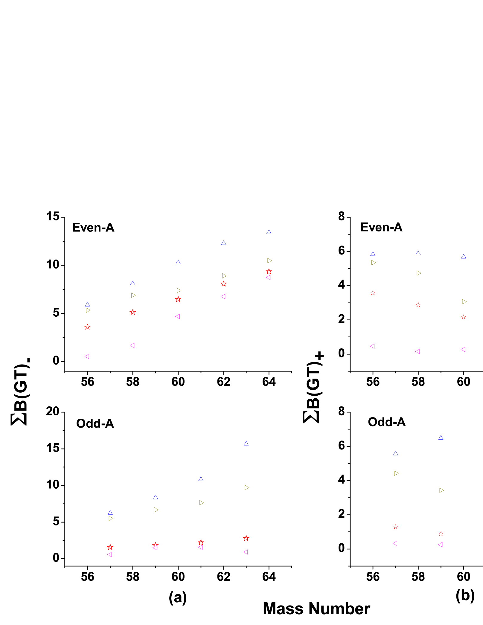
Figure 1: Total GT strength calculated in all four QRPA models. Even mass nuclei are shown in the upper panel. Lower panels depict the calculated strength for odd mass nuclei.

We present our calculated total GT strength distributions along with calculated centroids and widths in Figs. 1 - 3. Fig. 1 displays the calculated total GT strength for the four chosen QRPA models. The left panels show calculated strength along $\beta$-decay direction whereas the left panels show the same along electron capture direction. In order to highlight the effect of deformation we have divided our calculation into even mass (where the deformation parameter approaches zero) and odd mass isotopes of nickel as shown in Fig. 1. The spherical calculations lead to smaller strength functions. It can be seen that the highest strength is calculated by SM (C) model and lowest by PM (B). It is also to be noted that for odd mass nuclei the deformed calculations are significantly bigger than the spherical calculations (specially along $\beta$-decay direction). Our calculation indicates that incorporation of deformation into QRPA calculation lead to bigger GT strength values.

We calculated centroids and widths of calculated GT strength distributions (discrete in nature) in all our four QRPA models. Mathematically the centroid of the calculated GT strength distribution was calculated as

$$Centroid(BGT)_{\pm}=\frac{\sum_{j}E_{j}\times B_{j}(GT_{\pm})}{\sum_{j}B_{j}(GT)_{\pm}}.$$ (14)

where $E_{j}$ are the daughter excitation energies in units of MeV and $B_{j}(GT)_{\pm}$ are the calculated GT strength along electron capture and $\beta^{-}$ directions, respectively (in arbitrary units).

The width of ($GT_{\pm}$) strength distribution function was calculated using the formula

$$Width(BGT)_{\pm}=\sqrt{\frac{\sum(E_{j}-\overline{E}_{\pm})^{2}\times B_{j}(GT_{\pm})}{\sum B_{j}(GT)_{\pm}}}.$$ (15)

where the $\overline{E}_{\pm}$ are the centroids calculated as discussed above.

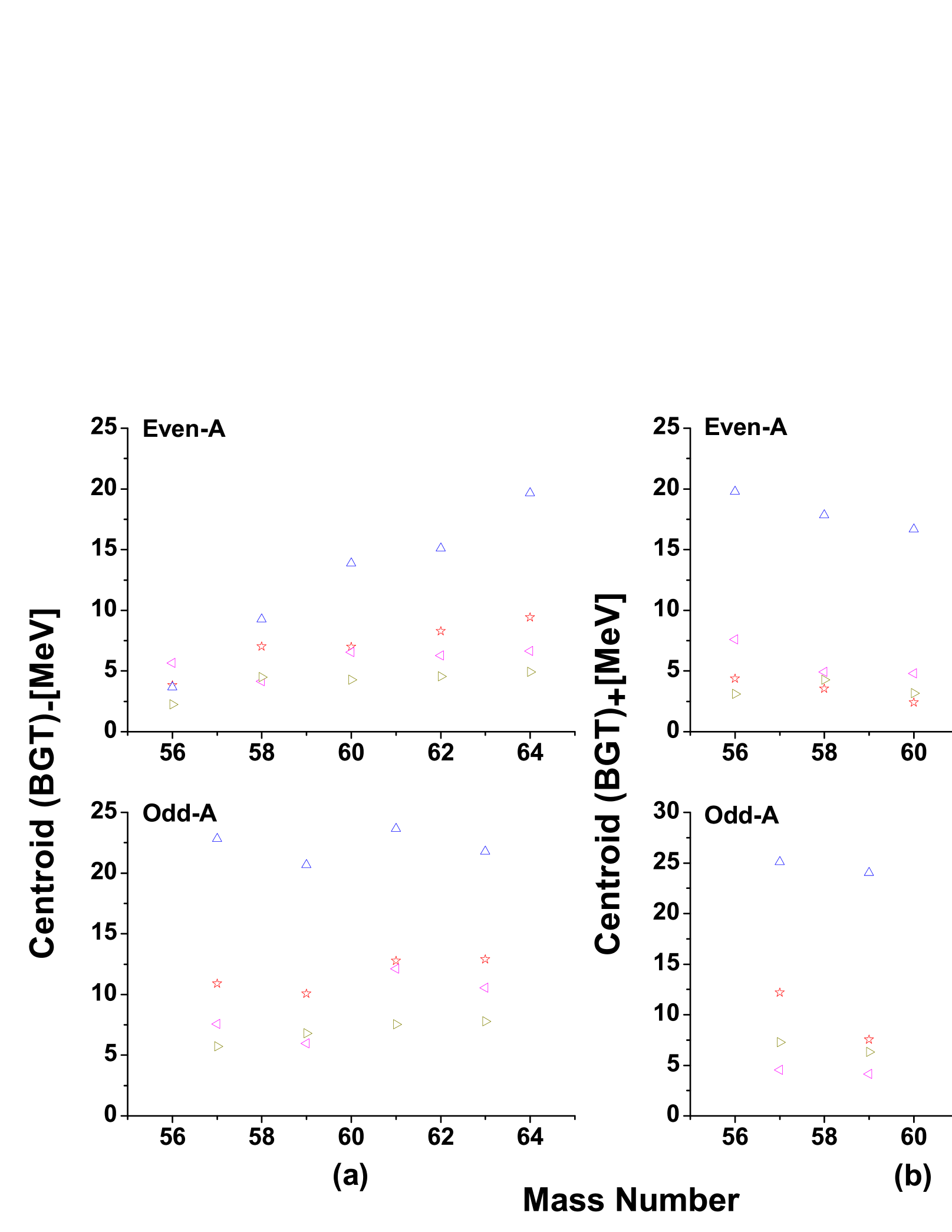
Figure 2: Comparison of centroid of calculated GT distributions, along $\beta$-decay and electron capture directions, in all four QRPA models.

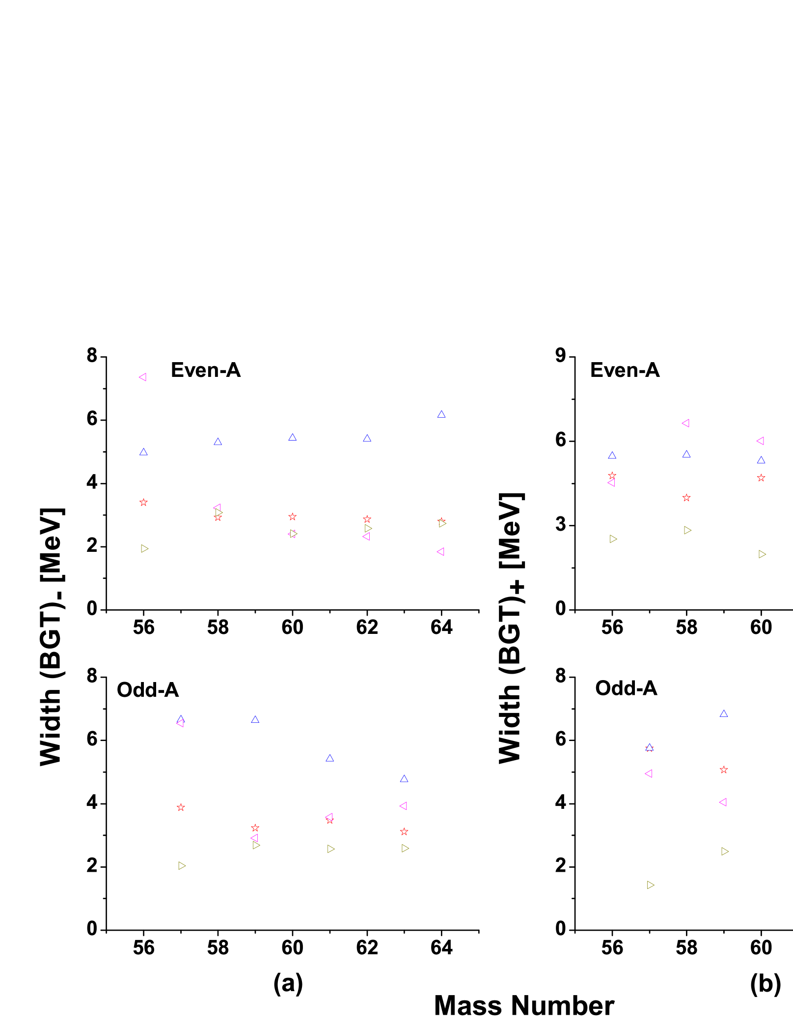
Figure 3: Comparison of width of calculated GT distributions, along $\beta$-decay and electron capture directions, in all four QRPA models.

Comparison of centroids is shown in Fig. 2. Here one notes that whereas both SM(C) and pn-QRPA(C) models calculated bigger GT strength, it is only the pn-QRPA(C) model in which the centroid of GT distributions resides at low excitation energy in daughter nucleus. This may transform to bigger weak-interaction rates once the phase space functions are incorporated in the calculations. SM(C) model in fact calculates biggest value of centroids of all the four models. The pn-QRPA(C) model also calculates smallest widths for the calculated GT strength distributions (Fig. 3).

The deviation of our calculated (re-normalized) Ikeda sum rule values from theoretically value is presented for both even and odd isotopes. In all our calculations, a quenching factor of $f_{q}^{2}$ = (0.6)² was used (as used normally in $fp$-shell calculations). The (re-normalized) Ikeda sum rule in all four models then transforms as

$$Re-ISR=B(GT)_{-}-B(GT)_{+}\cong 3f_{q}^{2}(N-Z).$$ (16)

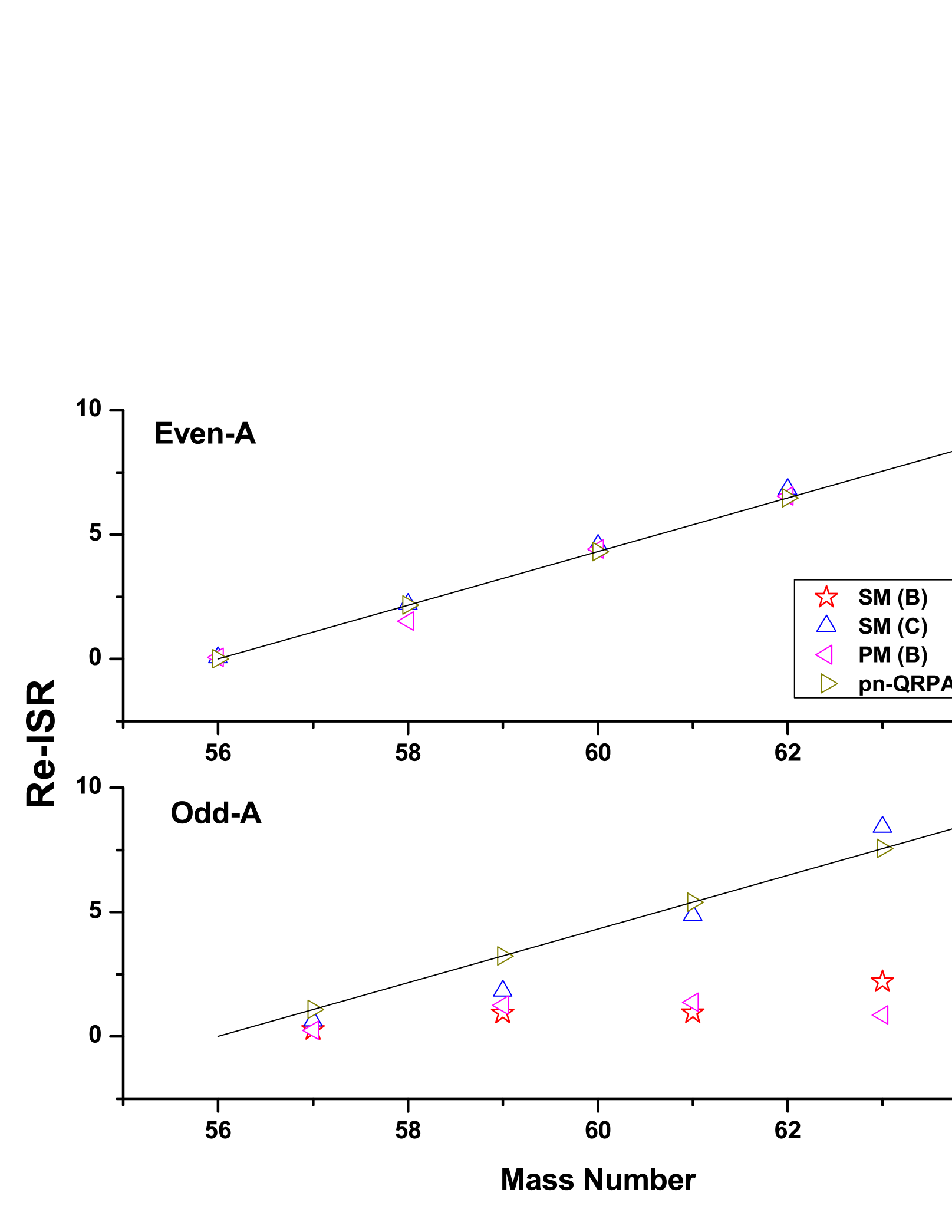
Figure 4: Comparison of calculated re-normalized Ikeda sum rule in all four QRPA models. Theoretically allowed sum rule is shown as a straight line to guide the eye.

In Fig. 4 the solid line shows the theoretical Ikeda sum rule value. If we treat nucleons as point particles and ignore two-body currents, the model independent Ikeda sum rule should be satisfied by all calculations. For even-A isotopes we get a decent agreement whereas for odd-A isotopes the spherical models fail. The pn-QRPA(C) model satisfies well the sum rule. The remaining three QRPA models struggle hard to satisfy the rule for odd-A cases. The deviations increase with increasing mass number for SM(B), PM(B) and SM(C) models. The $2p-2h$ configuration mixing can account for the missing strength in the PM and SM models (for further discussion see [30, 42]).

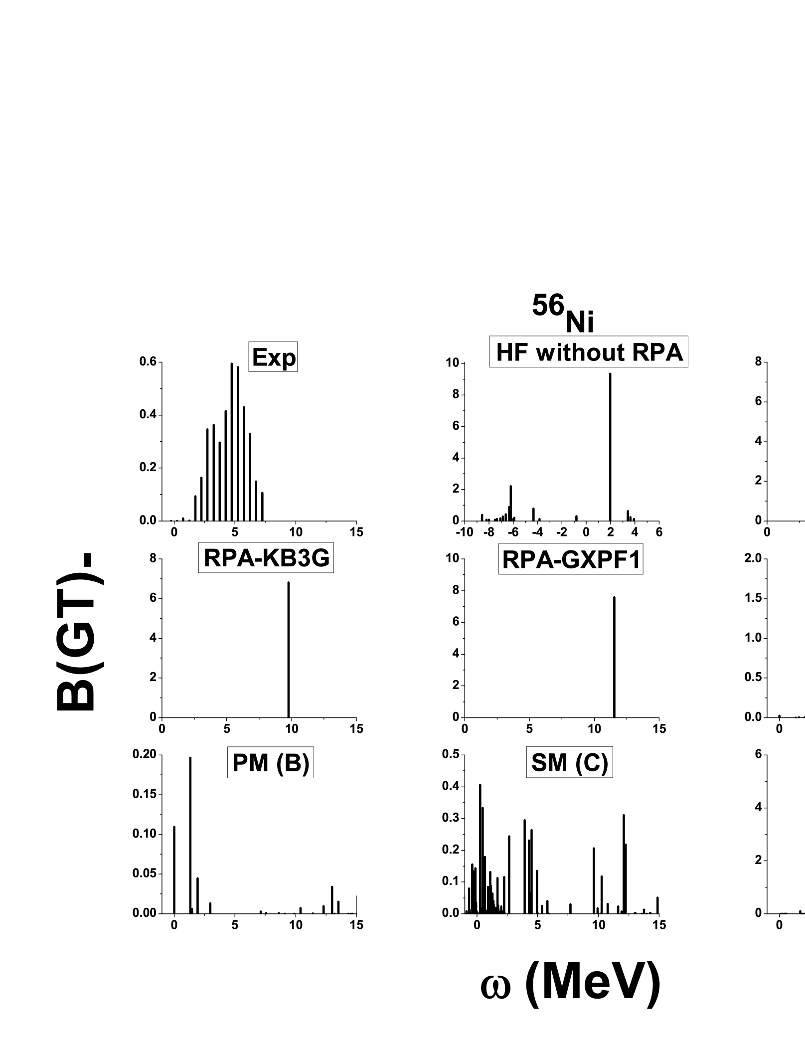
Figure 5: GT strength distributions in ⁵⁶Ni along $\beta$-decay direction. Exp shows measured distribution by [43]. Second panel on top shows the calculated unperturbed GT strength without RPA correlations by [44]. RPA calculations using shell model interactions – FDP6, KB3G and GXPF1 were taken from [8]. Last four panels depict calculated strength distributions using our four QRPA models. The abscissa represents energy in the daughter nucleus.

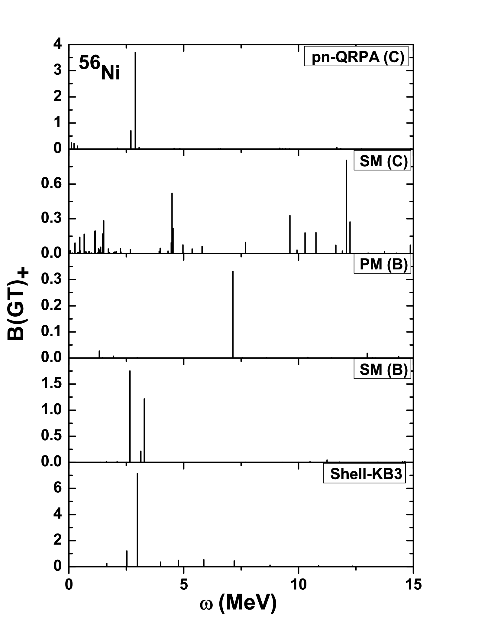
Figure 6: Calculated B(GT)₊ strength distributions in ⁵⁶Ni compared with shell model calculation [46]. The abscissa represents energy in the daughter nucleus.

After presenting a mutual comparison of the four QRPA models we next discuss how our calculated GT distributions compare with the previous calculations and measurements. Fig. 5 shows the B(GT)_- strength distributions in ⁵⁶Ni isotopes. On the experimental side we show the results of ⁵⁶Ni$(p,n)$ charge-exchange reaction [43] labeled Exp. We show the Hartree-Fock (HF) (unperturbed strength calculation) [44] and RPA calculation using shell model interactions- FDP6 [20], KB3G [19] and GXPF1 [45] performed by [8] in the next four panels of Fig. 5. The experimental data is not reproduced well by theoretical calculations for this doubly magic nucleus. Whereas RPA calculations put all strength in one transition, the other models do show a fragmented distribution. The centroids for the GT distribution calculated by SM (B), PM (B), SM (C) and pn-QRPA (C) models are 3.86 MeV, 5.65 MeV, 3.66 MeV and 2.26 MeV, respectively. These values are close to the experimental value of 4.1 MeV [43]. The RPA model calculates centroid values of 10.62 MeV, 9.77 MeV and 11.54 MeV with the FPD6, KB3G and GXPF1 interactions, respectively [8]. Calculated GT strength along the electron capture direction for ⁵⁶Ni is shown in Fig. 6. Here we compare our calculated GT distributions against the shell model (with KB3 interaction) calculation [46]. We note that shell model result is in very good agreement with the pn-QRPA (C) model calculation. SM (C) strength is well fragmented. Suzuki and collaborators [47] performed a shell model calculation of GT strength distributions and stellar electron capture rates of nickel isotopes. They used the KB3G and GXPF1J [48] interactions for their calculation. It was argued in their calculation that the GXPF1J interaction best reproduced the observed measured GT strength, specially for neutron-rich nickel isotopes. The cumulative GT strength distribution using the KB3G and GXPF1J interactions may be seen from Fig. 5 of [47]. The total GT strength calculated using the GXPF1J (KB3G) interaction was 6.2 (5.4). These strength values compare well with the total GT strength value of 5.34 calculated using the pn-QRPA(C) model.

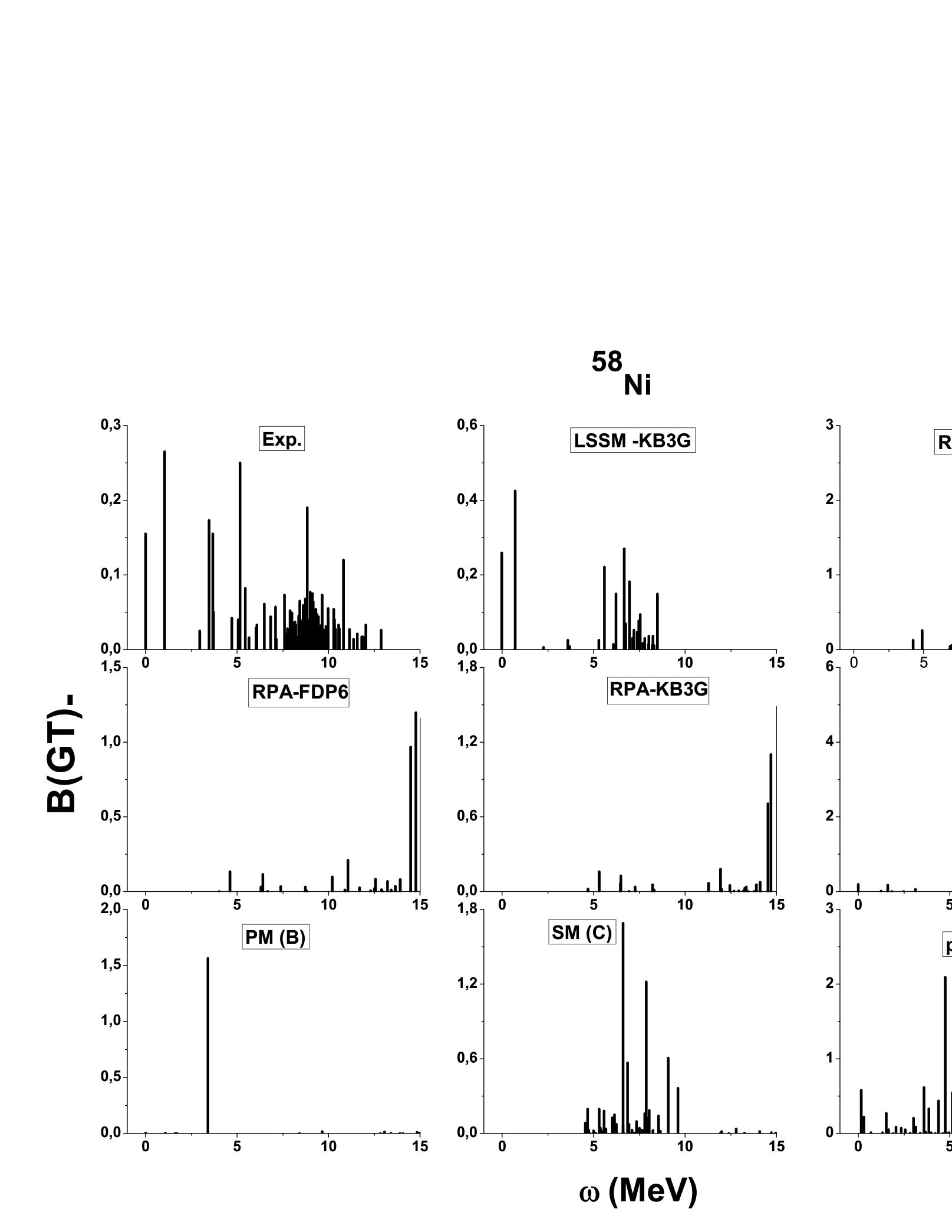
Figure 7: GT strength distributions in ⁵⁸Ni along $\beta$-decay direction. Exp. shows measured distribution by [17, 18]. Second panel on top shows the large scale shell model calculation by [22]. RPA calculations using shell model interactions – GXPF1, FPD6 and KB3G were taken from [8]. Last four panels depict calculated strength distributions using our four QRPA models. The abscissa represents energy in the daughter nucleus.

The B(GT)_- strength distributions in ⁵⁸Ni is presented in Fig. 7. The measured data was taken from the ⁵⁸Ni$(^{3}He,t)$ charge-exchange reaction [17, 18]. Here we also show the results of Large Scale Shell Model calculation (LSSM) with KB3G interaction [22] and RPA calculation with KB3G, FDP6 and GXPF1 interactions [8]. The comparison shows that the best agreement with experiment is seen in LSSM model. The pn-QRPA(C) model also fairly describe the low-lying measured data. The RPA calculation exhibits peaks at higher energies (around 14-16 MeV). In SM(B) and PM(B) models, only one main peak is seen.

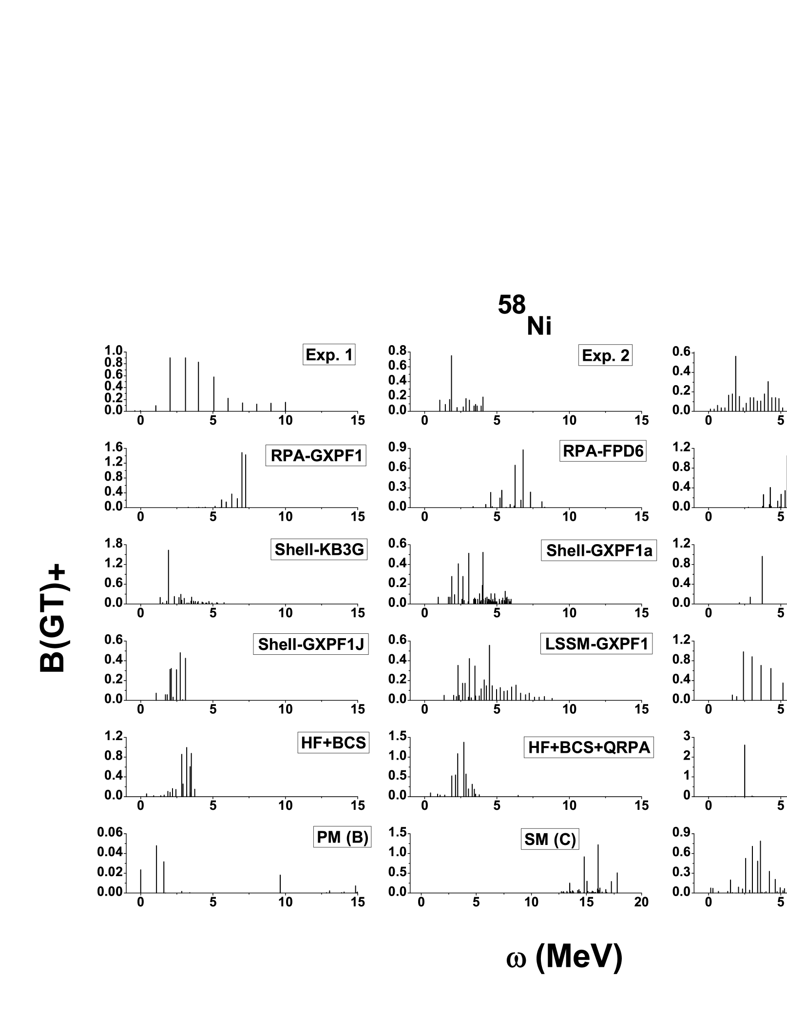
Figure 8: GT strength distributions in ⁵⁸Ni along electron capture direction. First row shows measured distributions by [15, 49, 16], respectively. Second row depicts RPA calculations using shell model interactions – FDP6, KB3G and GXPF1 taken from [8]. Third row presents shell model (employing KB3G and GXPF1a interactions) and QRPA calculations done by [52]. Fourth row shows shell model calculation using GXPF1J interaction by [47] and large scale shell model calculation using GXPF1 interaction by [16] and KB3 interaction by [22]. HF+BCS and HF+BCS+QRPA calculations were taken from [2]. Last four panels depict calculated strength distributions using our four QRPA models. The abscissa represents energy in the daughter nucleus.

We found a wealth of data for GT strength distribution of ⁵⁸Ni along the electron capture direction. We found three different measurement results displaying rather varying strength distributions. These are shown in top three panels of Fig. 8. The ⁵⁸Ni$(n,p)$ data at incident energy of 198 MeV is presented as Exp. 1 [15]. Exp. 2 shows the $(d,^{2}He)$ charge-exchange reactions performed by Hagemann et al. [49]. Exp. 3 depicts the ⁵⁸Ni$(t,^{3}He)$ charge-exchange reaction performed by Cole and collaborators [16] whereas Besides we present theoretical calculations of GT strength for ⁵⁸Ni using 15 different microscopic models. For references see caption of Fig. 8. Here we note that LSSM and pn-QRPA (C) are in reasonable agreement with the low-lying measured data. This very good comparison with experimental data can lead to very reliable estimate of stellar weak rates using the pn-QRPA(C) model.

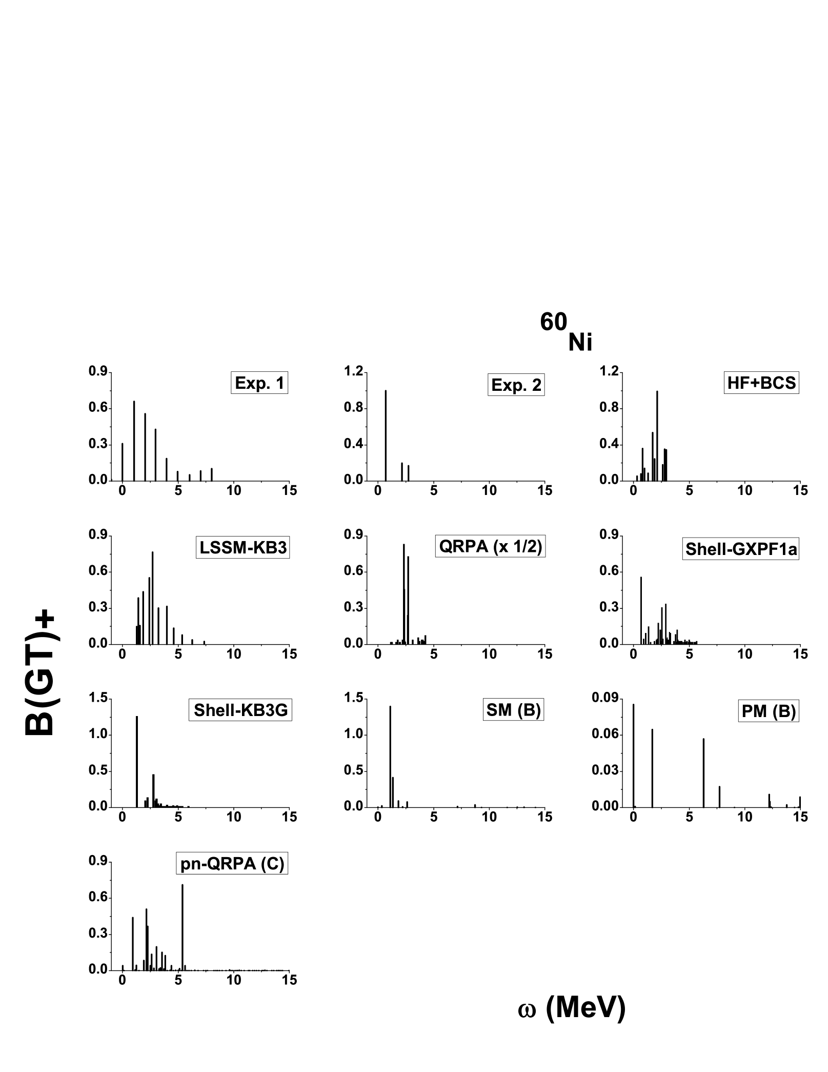
Figure 9: GT strength distributions in ⁶⁰Ni along electron capture direction. Exp. 1 shows measured distribution by [50] and Exp. 2 by [51]. HF+BCS and HF+BCS+QRPA calculations were taken from [2]. Large scale shell model calculation using KB3 interaction was taken from [22]. QRPA and shell model (employing KB3G and GXPF1a interactions) calculations were taken from [52] while those using GXPF1J interaction was taken from [47]. Last four panels depict calculated strength distributions using our four QRPA models. The abscissa represents energy in the daughter nucleus.

The B(GT)₊ distribution for ⁶⁰Ni was measured using $(n,p)$ reaction at 198 MeV by Williams and collaborators [50]. The result is shown as Exp. 1 in Fig. 9. Later Anantaraman et al. [51] studied the electron capture strength for ^60,62Ni using $(p,n)$ reactions at 134.3 MeV in inverse kinematics at a higher resolution. The authors reported differences in the two measurement results. Their findings are marked as Exp. 2 in Fig. 9. The next two panels show the HF approximation and HF+QRPA calculation built on a deformed selfconsistent mean field basis employing pairing correlations in BCS approximation [2]. The basis were obtained from two-body density-dependent Skyrme forces. This is followed by the large scale shell model calculation of [22]. The QRPA and shell model calculations (performed in a truncated $pf$ model space comprising of 5 holes in the $f_{7/2}$ shell using the GXPF1a and KB3G interactions) were taken from [52]. Shell model calculation [47] using the GXPF1J interaction is also shown. The last four panels show our QRPA results. It is noted that LSSM-KB3 calculation is in decent agreement with Exp. 1 whereas SM (B) is in good agreement with Exp. 2. The pn-QRPA(C) distribution is in good agreement with Exp. 1 till 5 MeV.

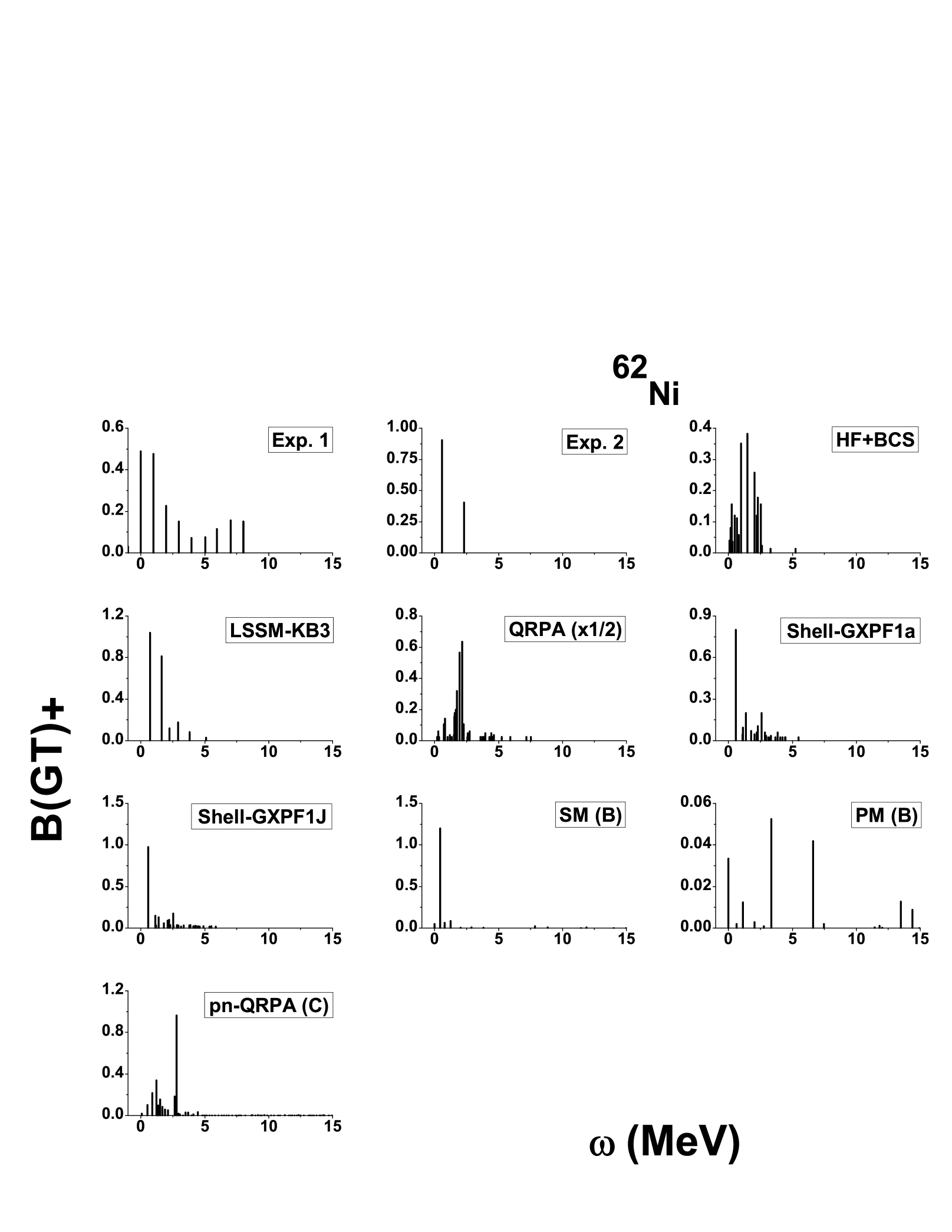
Figure 10: GT strength distributions in ⁶²Ni along electron capture direction. Exp. 1 shows measured distribution by [50] and Exp. 2 by [51]. HF+BCS and HF+BCS+QRPA calculations were taken from [2]. Large scale shell model calculation using KB3 interaction was taken from [22]. QRPA and shell model (employing KB3G and GXPF1a interactions) calculations were taken from [52]. Shell model calculation using GXPF1J interaction was taken from [47]. Last four panels depict calculated strength distributions using our four QRPA models. The abscissa represents energy in the daughter nucleus.

For ⁶²Ni isotope, measured and calculated B(GT)₊ distributions were taken from same sources as in Fig. 9. All the strength distributions are labeled same and presented in Fig. 10. The LSSM-KB3 data compares fairly good with Exp. 2 data. Among our four modes, it is the pn-QRPA (C) model which best describes the experimental data.

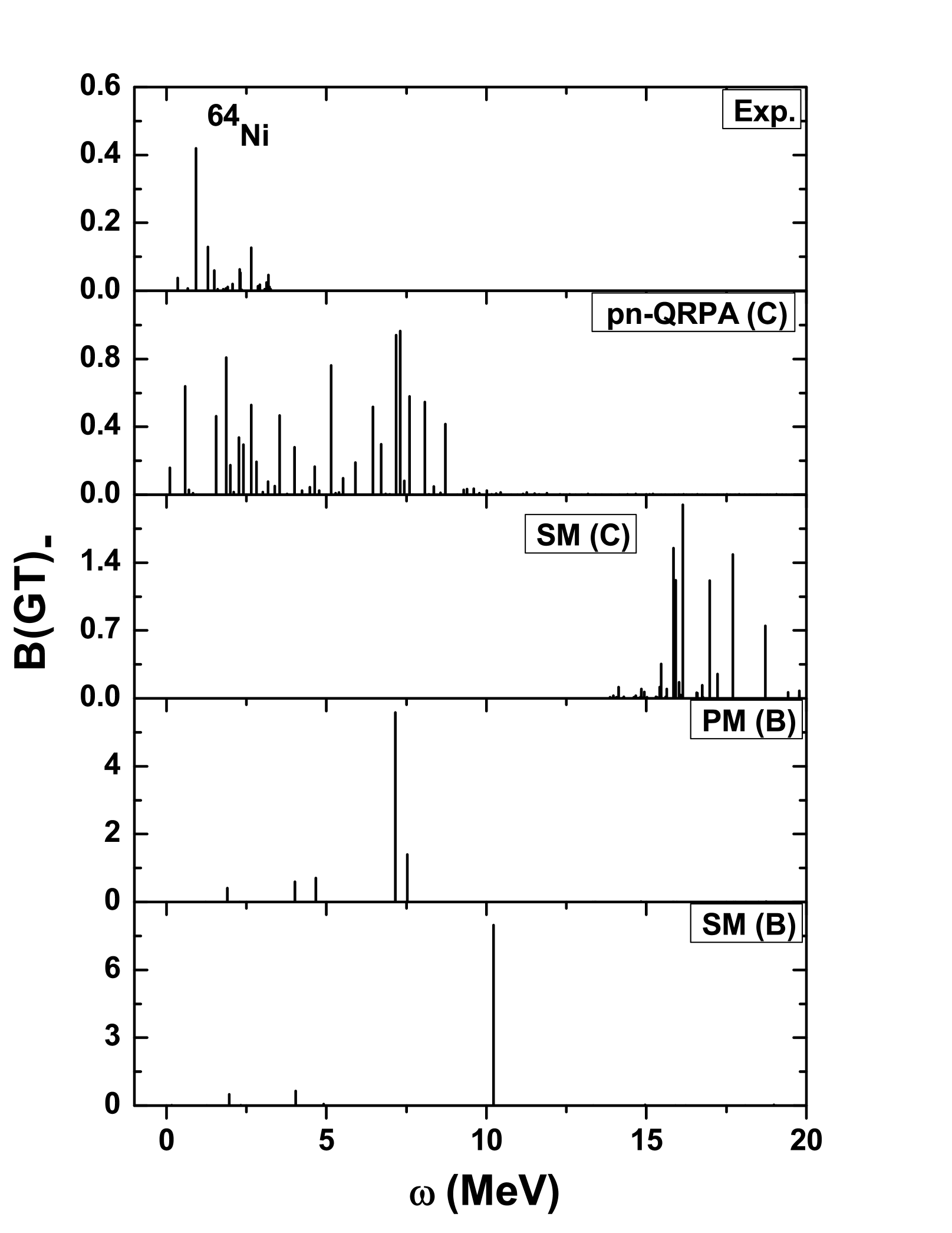
Figure 11: Calculated B(GT)_- strength distributions in ⁶⁴Ni compared with measured data [53]. The abscissa represents energy in the daughter nucleus.

In Fig. 11, our model calculations for B(GT)_- strength distributions in ⁶⁴Ni have been compared with the ⁶⁴Ni$(^{3}He,t)$ charge-exchange reaction at 140 MeV/nucleon [53]. Here we note that the pn-QRPA (C) model is in decent agreement with measured data in low-energy region. Remaining QRPA models calculate bulk of strength at high excitation energies in daughter.

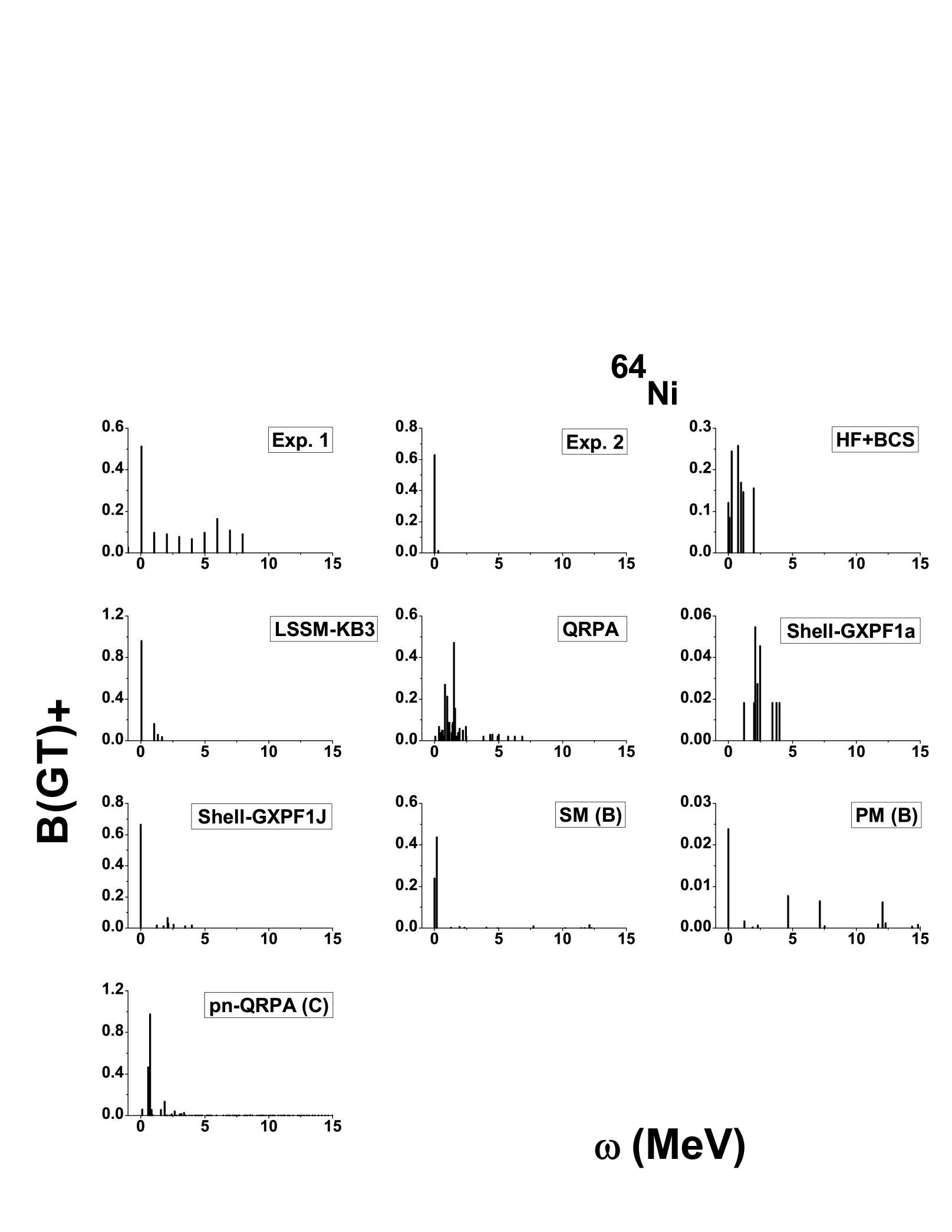
Figure 12: GT strength distributions in ⁶⁴Ni along electron capture direction. Exp. 1 shows measured distribution by [50] and Exp. 2 by [54]. HF+BCS and HF+BCS+QRPA calculations were taken from [2]. Large scale shell model calculation using KB3 interaction was taken from [22]. QRPA and shell model (employing KB3G and GXPF1a interactions) calculations were taken from [52]. Shell model calculation using GXPF1J interaction was taken from [47]. Last four panels depict calculated strength distributions using our four QRPA models. The abscissa represents energy in the daughter nucleus.

We present the ⁶⁴Ni$(n,p)$ [50] and ⁶⁴Ni$(d,^{2}He)$ data [54] in first two panels of Fig. 12. The remaining panels show theoretical calculations and are in same order as depicted in Fig. 10. Here one notes that LSSM-KB3 and pn-QRPA (C) model calculations are in good agreement with data of Exp. 1. The pn-QRPA (C) model calculates low-lying centroid as compared to PM (B), PM (C) and SM (C) models.

As mentioned earlier, with proceeding collapse the stellar density increases by orders of magnitude and the resulting electron chemical potential is significantly higher than the nuclear $Q$ value. Under prevailing conditions the stellar rates are largely determined by the total strength and centroid of the GT_± strength distributions. In Tables. 1 - 5 we present the total B(GT) strength, along $\beta^{-}$ and $\beta^{+}$ directions, and compare our calculated cumulative strength with previous calculations and measurements wherever possible. It is noted that in majority of the cases the total GT strength calculated by our pn-QRPA(C) model is in very good agreement with measured data.

It can be seen from Tab. 1 and Tab. 2 that the pn-QRPA(C) model calculates a bigger B(GT)_- strength of 5.34 for ⁵⁶Ni as compared to the measured ⁵⁶Ni$(p,n)$ data [43] of 3.8 units. Shell model and RPA calculations estimate even bigger values of total strength for ⁵⁶Ni. For ⁵⁸Ni and ⁶⁰Ni, the pn-QRPA(C) calculated total B(GT)_- strength is in excellent agreement with measured data. Our model calculates total strength of 6.89 units for the case of ⁵⁸Ni to be compared with the measured value of 7.4 [58]. In case of ⁶⁰Ni the calculated total strength value of 7.38 units is even closer to the measured value of 7.2 units [58]. For ⁶⁴Ni the measured total strength is 1.9 units in the $(^{3}He,t)$ experiment [53] up to 3.5 MeV excitation energy in daughter. The pn-QRPA(C) model calculated strength up to 3.5 MeV in ⁶⁴Cu is 3.7 units (in Tab. 2 the calculated value of 10.5 is up to 20 MeV in daughter nucleus).

The calculated and measured total B(GT)₊ strength values are shown in Tables. 3 - 5. Total strength for ⁵⁸Ni is shown in Tab. 3 and Tab. 4. The ⁵⁸Ni$(t,^{3}He,)$⁵⁸Co data [16] of 4.1 units is in very good agreement with our pn-QRPA (C) value of 4.73 units. Likewise for ⁶⁰Ni the measured total strength of 3.11 [50] compares excellent with the pn-QRPA(C) value of 3.06 units. For ⁶²Ni (⁶⁴Ni) the $(n,p)$ data gives a total strength of 2.5 (1.72) [50]. This is to be compared with the pn-QRPA(C) calculated value of 2.43 (1.86) units, respectively. It is noted that the spectral distribution [59] and shell model calculations (using vector method code, FPC8 and FPVH interactions) [50, 60] tend to overestimate the calculated strength. Remaining shell model calculations are, in general, very good agreement with measured data.

We finally present comparison of calculated and measured centroid values in Tab. 6 and Tab. 7. It is noted that the pn-QRPA(C) model places centroid at relatively low energies in daughter compared with other calculations. The centroid placement is also decent when compared with experimental data.

4 Summary and Conclusions

GT transitions for $fp$-shell nuclei play a leading role in the presupernova and supernova phases of massive stars. In this work, we calculated GT strength distribution functions for isotopes of nickel using microscopic QRPA methods (namely pn-QRPA, Schematic Model and Pyatov Method). Within this framework, we studied the role of deformed basis in QRPA methods. We did our calculations for 56$\leq$A$\leq$64.

Our calculations showed that the models with deformation of the nucleus incorporated gave better results for total GT strength and fulfillment of Ikeda sum rule as against those models performed in spherical basis. The pn-QRPA (C) model was found the best amongst the four models used. Not only were the model results in good agreement with measured data but it also resulted in placement of centroid at low excitation energies as compared to SM (C) model. Tab. 6 and Tab. 7 confirm the fact reported in [8] that the pn-QRPA (C) model places the centroid at much lower energies in daughter nuclei as compared to other RPA interactions. It was also concluded in [8] that GT centroid placement by the pn-QRPA (C) model is, in general, in very good agreement with the centroids of measured data. It was shown in the current work that not only the low-lying measured GT distribution was reproduced well by the pn-QRPA(C) model but also the calculated total GT strength and centroid placement were in decent agreement with measured data. Amongst all the RPA models the pn-QRPA(C) model is the clear choice and should be used for a reliable estimate of weak-interaction mediated rates in stellar environment.

Likewise, LSSM model results in very good agrement of calculated GT strength distributions with measured data. However the pn-QRPA (C) model has the additional feature that the model can be used for any arbitrary heavy nucleus. This advantage comes handy when GT strength distributions for hundreds of nuclei are required (including heavy ones) for modeling of various astrophysical phenomena.

Acknowledgments: J.-U. Nabi wishes to acknowledge the support provided by Tübitak (Turkey) under Program No. 1059B211402772, Higher Education Commission Pakistan through project number 5557/KPK/NRPU/R$\&$D/HEC/2016 and Pakistan Science Foundation through project number PSF-TUBITAK/KP-GIKI (02).

References:

Table 1: Total B(GT${}_{-})$ strength for nickel isotopes.

56Ni	$\sum B(GT)_{-}$
Exp. [43]	3.8
HFB with RPA [44]	18.28
RPA-GXPF1 [8]	7.58
RPA-FPD6 [8]	6.34
RPA-KB3G [8]	6.81
HF+RPA [57]	13.5
LSSM-KB [55]	11.4
Shell-GXPF1 [47]	6.2
Shell-GXPF1A [47]	6.2
Shell-GXPF1J [47]	6.2
Shell-KBF [47]	5.3
Shell-KB3G [47]	5.4
SM (B)	3.58
PM (B)	0.53
SM (C)	5.86
pn-QRPA (C)	5.34
57Ni
LSSM-KB [55]	14.0
SM (B)	1.56
PM (B)	0.57
SM (C)	6.2
pn-QRPA (C)	5.5
58Ni
Exp.1 [58]	7.4
Exp.2 [17, 18]	3.67
RPA-GXPF1 [8]	9.7
RPA-FPD6 [8]	7.96
RPA-KB3G [8]	8.51
Shell-GXP1J [21]	8.0
LSSM-KB [55]	15.8
Spect.Dist.(configuration) [59]	19.33
Spect.Dist.(scalar) [59]	18.03
Shell Model [60]	16.6
LSSM-KB3 [22]	7.7
pn-QRPA [2]	16.46

Table 2: Same as Table 1.

58Ni	$\sum B(GT)_{-}$
SM (B)	5.12
PM (B)	1.67
SM (C)	8.09
pn-QRPA (C)	6.89
60Ni
Exp. [58]	7.2
Shell-GXP1J [21]	9.9
LSSM-KB3 [22]	10
pn-QRPA [2]	19.71
Spect.Dist.(configuration) [59]	23.51
Spect.Dist.(scalar) [59]	21.62
Shell Model [60]	24.6
SM (B)	6.45
PM (B)	4.69
SM (C)	10.27
pn-QRPA (C)	7.38
62Ni
pn-QRPA [2]	22.77
SM (B)	8.07
PM (B)	6.75
SM (C)	12.29
pn-QRPA (C)	8.9
64Ni
Exp. [53]	1.9
pn-QRPA [2]	27.24
SM (B)	9.35
PM (B)	8.75
SM (C)	13.4
pn-QRPA (C)	10.5

Table 3: Total B(GT${}_{+})$ strength for nickel isotopes.

56Ni	$\sum B(GT)_{+}$
RPA-GXPF1 [8]	7.58
RPA-FPD6 [8]	6.34
RPA-KB3G [8]	6.81
LSSM-KB [55]	11.4
Shell-GXPF1[47]	6.2
Shell-GXPF1A[47]	6.2
Shell-GXPF1J[47]	6.2
Shell-KBF[47]	5.3
Shell-KB3G[47]	5.4
SMMC [56]	9.86
SM (B)	3.57
PM (B)	0.46
SM (C)	5.83
pn-QRPA (C)	5.34
57Ni
LSSM-KB [55]	10.9
SM (B)	1.29
PM (B)	0.33
SM (C)	5.56
pn-QRPA (C)	4.42
58Ni
Exp.1 [15]	3.8
Exp.2 [49]	2.04
Exp.3 [16]	4.1
RPA-GXPF1 [8]	6.09
RPA-FPD6 [8]	4.36
RPA-KB3G [8]	4.91
Shell-GXP1J [21]	4.7
LSSM-KB[55]	9.5
LSSM-KB3[22]	4.4
SMMC [56]	6.72
Shell-FPC8 [50]	12.17
Shell-FPVH [50]	12.28
Spect.Dist.(configuration) [59]	13.33
Spect.Dist.(scalar) [59]	12.03
Shell Model [60]	10.6

Table 4: Same as Table 3.

58Ni	$\sum B(GT)_{+}$
HF+BCS [2]	6.19
pn-QRPA [2]	5.00
Shell-GXPF1[47]	4.7
Shell-GXPF1A[47]	4.7
Shell-GXPF1J[47]	4.7
Shell-KBF[47]	4.2
Shell-KB3G[47]	4.0
GXPF1 [16]	4.1
SM (B)	2.87
PM (B)	0.15
SM (C)	5.88
pn-QRPA (C)	4.73
60Ni
Exp. [50]	3.11
Shell-GXP1J [21]	3.4
Spect.Dist.(configuration) [59]	11.51
Spect.Dist.(scalar) [59]	9.62
Shell Model [60]	12.6
SMMC [56]	5.18
Shell-FPC8 [50]	9.79
Shell-FPVH [50]	9.86
LSSM-KB3 [22]	3.4
HF+BCS [2]	4.97
pn-QRPA [2]	3.72
Shell-GXPF1[47]	3.4
Shell-GXPF1A[47]	3.4
Shell-GXPF1J[47]	3.4
Shell-KBF[47]	3.1
Shell-KB3G[47]	2.8
SM (B)	2.17
PM (B)	0.27
SM (C)	5.68
pn-QRPA (C)	3.06

Table 5: Same as Table 3.

62Ni	$\sum B(GT)_{+}$
Exp. [50]	2.5
Shell-FPC8 [50]	7.67
Shell-FPVH [50]	7.29
Shell-GXPF1[47]	2.0
Shell-GXPF1A[47]	1.9
Shell-GXPF1J[47]	1.9
Shell-KBF[47]	2.0
Shell-KB3G[47]	2.0
LSSM-KB3 [22]	2.1
HF+BCS [2]	3.40
pn-QRPA [2]	2.36
SMMC [56]	3.43
SM (B)	1.53
PM (B)	0.2
SM (C)	5.46
pn-QRPA (C)	2.43
64Ni
Exp. 1 [50]	1.72
Exp. 2 [54]	1.18
Shell-FPC8 [50]	5.1
Shell-FPVH [50]	4.57
Shell-GXPF1[47]	1.0
Shell-GXPF1A[47]	0.9
Shell-GXPF1J[47]	0.9
Shell-KBF[47]	1.2
Shell-KB3G[47]	1.1
LSSM-KB3 [22]	1.3
HF+BCS [2]	2.65
pn-QRPA [2]	1.65
SMMC [56]	1.73
SM (B)	0.73
PM (B)	0.06
SM (C)	4.76
pn-QRPA (C)	1.86

Table 6: Centroid values of GT strength distributions in even-even nickel isotopes.

56Ni	$\bar{E}_{m}$ [MeV]	$\bar{E}_{p}$ [MeV]
Exp. [43]	4.1	-
RPA-GXPF1 [8]	11.54	11.54
RPA-FPD6 [8]	10.62	10.62
RPA-KB3G [8]	9.77	9.77
Shell-KB3G [46]	6.0	-
SMMC [61]	-	2.6
FFN [3]	-	3.78
Shell-GXPF1 [47]	-	5.2
Shell-GXPF1A [47]	-	5.2
Shell-GXPF1J [47]	-	5.0
Shell-KBF [47]	-	4.4
Shell-KB3G [47]	-	3.7
SM (B)	3.86	4.36
PM (B)	5.65	7.58
SM (C)	3.66	19.76
pn-QRPA (C)	2.26	3.11
58Ni
Exp.1 [15]	-	4.0
Exp.2 [16]	-	4.4
Exp.3 [58]	9.4	-
RPA-GXPF1 [8]	14.6	6.79
RPA-FPD6 [8]	13.94	6.15
RPA-KB3G [8]	13.97	5.02
SMMC [61]	-	2.0
LSSM-KB3 [22]	-	3.75
FFN [3]	6.5	3.76
Shell-GXPF1 [47]	-	4.2
Shell-GXPF1A [47]	-	4.3
Shell-GXPF1J [47]	-	4.1
Shell-KBF [47]	-	3.7
Shell-KB3G [47]	-	2.9
SM (B)	7.01	3.54
PM (B)	4.15	4.93
SM (C)	9.27	17.82
pn-QRPA (C)	4.48	4.27

Table 7: Same as Table 6.

60Ni	$\bar{E}_{m}$ [MeV]	$\bar{E}_{p}$ [MeV]
Exp. [58]	9.0	-
SMMC [61]	-	1.0
FFN [3]	4.9	2.0
LSSM-KB3 [22]	-	2.88
Shell-GXPF1 [47]	-	3.0
Shell-GXPF1A [47]	-	3.1
Shell-GXPF1J [47]	-	2.8
Shell-KBF [47]	-	2.7
Shell-KB3G [47]	-	2.4
SM (B)	6.97	2.39
PM (B)	6.54	4.8
SM (C)	13.87	16.67
pn-QRPA (C)	4.27	3.18
62Ni
LSSM-KB3 [22]	-	1.78
FFN [3]	-	2.0
Shell-GXPF1 [47]	-	1.8
Shell-GXPF1A [47]	-	2.0
Shell-GXPF1J [47]	-	1.8
Shell-KBF [47]	-	1.7
Shell-KB3G [47]	-	1.5
SM (B)	8.27	1.76
PM (B)	6.28	5.77
SM (C)	15.09	13.39
pn-QRPA (C)	4.55	2.28
64Ni
LSSM-KB3 [22]	-	0.5
FFN [3]	-	2.0
Shell-GXPF1 [47]	-	0.8
Shell-GXPF1A [47]	-	0.9
Shell-GXPF1J [47]	-	0.8
Shell-KBF [47]	-	0.5
Shell-KB3G [47]	-	0.5
SM (B)	9.41	1.29
PM (B)	6.63	6.68
SM (C)	19.66	13.68
pn-QRPA (C)	4.93	1.0

References

- [1] D. Arnett, Supernovae and Nucleosynthesis, Princeton Univ. Press, 1996.
- [2] P. Sarriguren, E. Moya de Guerra, R. Alvarez-Rodriguez, Nucl. Phys. A, 716, 230, 2003.
- [3] G. M. Fuller et al., Astrophys. J., 42, 447, 1980.
- [4] M. B. Aufderheide, I. Fushiki, S. E. Woosley, E. Stanford, D. H. Hartmann, Astrophys. J. Suppl. Ser., 91, 389, 1994.
- [5] J.-U. Nabi, H. V. Klapdor-Kleingrothaus, Eur. Phys. J. A, 5, 337, 1999.
- [6] K. Langanke, G. Martínez-Pinedo,Nucl. Phys. A, 673, 481, 2000.
- [7] J.-U. Nabi, H. V. Klapdor-Kleingrothaus, At. Data Nucl. Data Tables, 88, 237, 2004.
- [8] J.-U. Nabi, C. W. Johnson, J. Phys. G: Nucl. Part. Phys.,40, 065202, 2013.
- [9] A. Heger, S. E. Woosley, G. Martínez-Pinedo, K. Langanke, Astrophys. J., 560, 307, 2001.
- [10] M. Bernas et al., Z. Phys. A, 336, 41, 1990.
- [11] F. Ameil et al., Eur. Phys. J. A, 1, 275, 1998.
- [12] S. Franchoo et al., Phys. Rev. Lett., 81, 3100, 1998.
- [13] F. Brachwitz, Astrophys. J., 536, 934, 2000.
- [14] M. Sasano, Phys. Rev. Lett., 107, 202501-1, 2011.
- [15] S. El-Kateb et al., Phys. Rev. C, 49, 3128, 1994.
- [16] A. L. Cole et al., Phys. Rev. C, 74, 034333, 2006.
- [17] Y. Fujita et al., Eur. Phys. J. A, 13, 411, 2002.
- [18] Y. Fujita et al., Phys. Rev. C, 75, 034310, 2007.
- [19] A. Poves, J. Sánchez-Solano, E. Caurier, F. Nowacki, Nucl. Phys A, 694, 157, 2001.
- [20] W. A. Richter, M. G. Van der Merwe, R. E. Julies, B. A. Brown, Nucl. Phys A, 523, 325, 1991.
- [21] T. Suzuki, M. Honma, K. Higashiyama, T. Yoshida, T. Kajino, T. Otsuka, H. Umeda, K. Nomoto, Phys. Rev. C, 79, 061603, 2009.
- [22] C. Caurier, K. Langanke, G. Martínez-Pinedo and F. Nowacki, Nucl. Phys. A, 653, 439, 1999.
- [23] J.-U. Nabi, H. V. Klapdor-Kleingrothaus, At. Data Nucl. Data Tables, 71, 149, 1999.
- [24] M-Ur Rahman, Astro. Space Sci., 355, 123, 2014.
- [25] J. A. Halbleib, R. A. Sorensen, Nucl. Phys. A, 98, 542, 1967.
- [26] J. Krumlinde, P. Möller, Nucl. Phys. A, 417, 419, 1984.
- [27] N. I. Pyatov, D. Salamov D, Nucleonica, 22, 127, 1977.
- [28] T. Babacan , D. I. Salamov, A. Kucukbursa, Phys. Rev. C, 71, 037303, 2005.
- [29] T. Babacan , D. I. Salamov, A. Kucukbursa, Math. Comp. Application, 10, 359, 2005.
- [30] S. Cakmak, J.-U. Nabi, T. Babacan, C. Selam, Astro. Space Sci., 352, 645, 2014.
- [31] N. Cakmak, S. Unlu, C. Selam, Ind. Acad. Sci., 75, 649, 2010.
- [32] D. I. Salamov et al., Proceedings of 5th Conference on Nuclear and Particle Physics (NUPPAC 05) (Cairo, August 2006), 361, 2006.
- [33] I. Ikeda, Prog. Theor. Phys., 31, 434, 1964.
- [34] D. I. Salamov, A. Kucukbursa, I. Maras, H. A. Aygor, T. Babacan, H. Bircan, Acta Phys. Slov., 53, 307, 2003.
- [35] C. Selam, T. Babacan, H. Bircan, H. A. Aygor, A. Kucukbursa, I. Maras, Math. Comput. Appl., 9, 79, 2004.
- [36] K. Muto, E. Bender, T. Oda and H. V. Klapdor-Kleingrothaus, Z. Phys. A, 341, 407, 1992.
- [37] M. Hirsch, A. Staudt, K. Muto, H. V. Klapdor-Kleingrothaus, At. Data Nucl. Data Tables, 53, 165, 1993.
- [38] S. Raman et al., At. Data Nucl. Data Tables, 36, 1, 1987.
- [39] P. Möller, J. R. Nix, At. Data Nucl. Data Tables, 26, 165, 1981.
- [40] G. Audi et al., Chin. Phys. C, 36, 1287, 2012.
- [41] M. Wang et al., Chin.Phys. C, 36, 1603, 2012.
- [42] S. Cakmak, J.-U. Nabi, T. Babacan, I. Maras, Adv. Space Res., 55, 440, 2015.
- [43] M. Sasano et al., Phys. Rev. C, 86, 034324, 2012.
- [44] C. L. Bai et al., Phy. Let. B, 719, 121, 2013.
- [45] M. Honma, T. Otsuka, B. A. Brown, T. Mizusaki, Phys. Rev. C, 65, 061301(R); 69, 034335, 2004.
- [46] K. Langanke, G. Martínez-Pinedo, Phys. Lett. B, 436, 19, 1998.
- [47] T. Suzuki et al., Phys. Rev. C, 83, 044619, 2011.
- [48] M. Honma et al., J. Phys. Conf. Ser. 20, 7, 2005.
- [49] M. Hagemann et al., Phys. Lett. B, 579, 251, 2004.
- [50] A. L. Williams et al., Phys. Rev. C, 51, 1144, 1995.
- [51] N. Anantaraman et al., Phys. Rev. C, 78, 065803, 2008.
- [52] A. L. Cole et al., Phys. Rev. C, 86, 015809, 2012.
- [53] L. Popescu et al., J. Phys. G: Nucl. Part. Phys., 31, (2005) S1945, 2005.
- [54] L. Popescu et al., Phys. Rev. C, 75, 054312, 2007.
- [55] H. Nakada, T. Sebe, J. Phys. G: Nucl. Part. Phys., 22, 1349, 1996.
- [56] K. Langanke et al., Phys. Rev. C, 52, 718, 1995.
- [57] I. Hamamoto, H. Sagawa, Phys. Rev. C, 48, R960, 1993.
- [58] J. Rapaport et al., Nucl. Phys. A, 410, 371, 1983.
- [59] S. Sarkar and K. Kar, J. Phys. G, 14, L123, 1988.
- [60] S. D. Bloom, G. M. Fuller, Nucl. Phys. A, 440, 511, 1985.
- [61] D. J. Dean et al., Phys. Rev. C, 58, 536, 1998.