A Canonical Construction of the Extended
Hilbert Space for Causal Fermion Systems

Abstract.

It is shown that second variations of the causal action can be decomposed into a sum of three terms, two of which being positive and one being small. This gives rise to an approximate decoupling of the linearized field equations into the dynamical wave equation and bosonic field equations. A concrete construction of homogeneous and inhomogeneous solutions of the dynamical wave equation in time strips is presented. In addition, it is show that the solution space admits a positive definite inner product which is preserved under the time evolution. Based on these findings, a canonical construction of the extended Hilbert space containing these solutions is given.

1. Introduction

The theory of causal fermion systems is a recent approach to fundamental physics (see the basics in Section 2, the textbooks [10, 21] or the website [1]). In this approach, all spacetime structures are encoded in a family of one-particle wave functions, referred to as the physical wave functions. The physical equations are formulated via the so-called causal action principle, a nonlinear variational principle where an action ${\mathcal{S}}$ is minimized under variations of all physical wave functions. If one describes the Minkowski vacuum, the physical wave functions can be identified with all the negative-energy solutions of the Dirac equation. In this way, Dirac’s original concept of the Dirac sea is incorporated. Likewise, a non-interacting system involving particles and/or anti-particles is described by including Dirac solutions of positive frequency (giving rise to additional one-particle states describing particles) and/or by removing Dirac solutions of negative energy (giving rise to “holes in the Dirac sea” describing anti-particles). If the interaction as described by the causal action principle is taken into account, the system is no longer composed of Dirac solutions, making it necessary to describe the whole family of physical wave functions in the realm of many-particle quantum theory (we refer the interested reader to the recent papers [19] and [5]). Nevertheless, even in the interacting situation, the physical wave functions still give a sensible notion of “one-particle wave functions.”

The problem to be addressed in this paper can be understood already in the non-interacting situation. Namely, in this case, the physical wave functions forming the causal fermion system span only a proper subspace of the Dirac solution space. More precisely, in the Minkowski vacuum, the physical wave functions are only the negative-frequency solutions, but the solutions of positive frequency are not part of the causal fermion system. While this minimalistic description is fully satisfying from the conceptual point of view, it is not sufficient for getting the connection to the description of the dynamics in terms of the standard physical equations. In the simplest case, in order to develop the perturbation theory for Dirac wave functions, one needs Green’s operators, whose construction makes it necessary to know the whole solution space (both positive and negative frequencies). With this in mind, one would like to extend the Hilbert space of physical wave functions of a causal fermion system to a larger Hilbert space, which for systems in Minkowski space also includes all solutions of positive frequency. Indeed, this extended Hilbert space was first constructed in [18], and it was used in subsequent papers [16, 19, 14].

The construction of the extended Hilbert space in [18] has the shortcoming that it is not manifestly canonical. This can be understood from the fact that it is based on linear perturbations of the system, parametrized by so-called compatible generators (see [18, Definition 5.2]). The resulting compatibility conditions are shown to be solvable (see [18, Section 5.2]), but it is not clear in general if the solutions are unique. This means that, depending on which generators are chosen, one might get different extended Hilbert spaces with potentially different dynamics. Clearly, this situation is not satisfying from the conceptual point of view. Therefore, it is an important task to improve the construction of the extended Hilbert space in such a way that it becomes independent of the choices of compatible generators. It is the main objective of the present paper to provide such a canonical construction.

Compared to the state of knowledge when the paper [18] was written, there is one new result on the structure of the causal action principle which inspired and will be crucial for our constructions: an approximate decoupling of the linearized field equations into the dynamical wave equation and a bosonic field equation. This approximate decoupling is based on the observation that second variations of the causal action principle can be written as a sum of three terms, the first two being non-negative, and the third being small. Linearized fields lie in the kernel of the second variations. Since the first two terms have the same sign, this means that they must both be zero, except for the coupling described by the third term. This is what we mean by “approximate decoupling” of the linearized field equations. Clearly, this statement needs to be made precise and formulated in mathematical terms. This will be worked out in detail in this paper (Sections 3–5). Although being a quite remarkable result of independent interest, the approximate decoupling will serve for us as a preparation for the construction of the extended Hilbert space (Sections 6 and 7).

We now explain a few constructions and ideas in more detail. The approximate decoupling of the linearized field equations can be understood in non-technical terms as follows. We first note that, assuming that the vacuum measure $\rho$ is a minimizer of the causal action principle, second variations of the causal action are always non-negative (for details and consequences see [11]). Solutions of the linearized field equations correspond to first variations which preserve criticality, meaning that the corresponding second variations $\delta^{2}{\mathcal{S}}$ of the causal action vanish. With this in mind, in this paper we always restrict attention to the kernel of $\delta^{2}{\mathcal{S}}$. This also implies that the positivity statements in [11] will not be of use. Instead, our argument is based on the observation that the second variations $\delta^{2}{\mathcal{S}}$ can be written as a sum of three terms,

$$\delta^{2}{\mathcal{S}}=\delta^{2}{\mathcal{S}}^{\text{\rm{lfe}}}+\delta^{2}{\mathcal{S}}^{Q}+{\mathcal{R}}\>.$$ (1.1)

the first two of which are non-negative, whereas the third summand (the “remainder”) is very small. The positivity of the first summand follows directly from the structure of the causal Lagrangian, being composed of sums of positive terms squared,

$$\frac{1}{4n}\sum_{i,j=1}^{2n}\Big{(}\big{|}\lambda^{xy}_{i}\big{|}-\big{|}\lambda^{xy}_{j}\big{|}\Big{)}^{2}$$

(basics on causal fermion systems and the causal action principle will be provided in Section 2.1 below). If each of the two factors of the square is varied linearly, we obtain the non-negative term

$$\delta^{2}{\mathcal{L}}^{\text{\rm{lfe}}}(x,y):=\frac{1}{4n}\sum_{i,j=1}^{2n}\delta\Big{(}\big{|}\lambda^{xy}_{i}\big{|}-\big{|}\lambda^{xy}_{j}\big{|}\Big{)}\>\delta\Big{(}\big{|}\lambda^{xy}_{i}\big{|}-\big{|}\lambda^{xy}_{j}\big{|}\Big{)}\geq 0\>,$$ (1.2)

and integrating $x$ and $y$ over spacetime gives a positive functional $\delta^{2}{\mathcal{S}}^{\text{\rm{lfe}}}\geq 0$.

The positivity of $\delta^{2}{\mathcal{S}}^{Q}$ is less obvious. This structural property of the causal action was observed only recently, based on the constructions in [12]. It provides the main new insight compared to the earlier constructions in [18]. Presenting this positivity property and working out some of its consequences is one of the main objectives of the present paper. The starting point is to consider the first variation $\delta\psi$ of one physical wave function $\psi$. The corresponding first variation of the causal Lagrangian can be written as

$$\delta{\mathcal{L}}(x,y)=-2\operatorname{Re}\Big{(}\mbox{$\prec\!\!$ \nolinebreak}\delta\psi(x)\>Q(x,y)\,\psi(y)\mbox{\nolinebreak$\succ$}+\mbox{$\prec\!\!$ \nolinebreak}\psi(x)\>Q(x,y)\,\delta\psi(y)\mbox{\nolinebreak$\succ$}\Big{)}$$ (1.3)

(see [12, eq. (3.8)] or (2.15) in Section 2.3; for details we refer again to Section 2). This formula can be understood immediately from the fact that $\delta{\mathcal{L}}(x,y)$ is real and that it is real-linear in both $\psi$ and $\delta\psi$. The main point is that the kernel $Q(x,y)$ is zero unless $x$ and $y$ are close together. Therefore, the first variation $\delta L(x,y)$ vanishes if the supports of $\psi$ and its variation $\delta\psi$ are vary far apart. We refer to such variations as variations with separated supports. They will be introduced systematically in Section 3, where we also clarify the notions of “close together” and “far apart” by discussing the relevant length scales. Varying once again, we again get zero, unless the second variation changes the factors $\psi$ in (1.3) to $\delta\psi$. We conclude that, for second variations with separated supports,

$$\delta^{2}{\mathcal{L}}(x,y)=-4\operatorname{Re}\mbox{$\prec\!\!$ \nolinebreak}\delta\psi(x)\>Q(x,y)\,\delta\psi(y)\mbox{\nolinebreak$\succ$}\>.$$ (1.4)

Integrating over $x$ and $y$ and using that second variations of the causal action are always non-negative (following the arguments in [11]), we conclude that

$$0\leq\delta^{2}{\mathcal{S}}^{Q}:=-4\int_{M}d\rho(x)\int_{M}d\rho(y)\>\mbox{$\prec\!\!$ \nolinebreak}\delta\psi(x)\>Q(x,y)\,\delta\psi(y)\mbox{\nolinebreak$\succ$}$$ (1.5)

(here the real part could be omitted because taking the complex conjugate corresponds to interchanging the integration variables $x\leftrightarrow y$). This positivity statement holds for any choice of $\delta\psi$, showing that the corresponding summand in (1.1) is also non-negative for general variations.

All contributions to the second variation which are neither of the form (1.2) nor of the form (1.4) are subsumed in the remainder term ${\mathcal{R}}$ in (1.1). These contributions are small as a consequence of the fact that they contain either an unvaried factors $(|\lambda^{xy}_{i}|-|\lambda^{xy}_{j}|)$ or else a factor $\kappa$ (coming from the second summand of the causal Lagrangian (2.1)). Here “small” means that, for systems describing Minkowski space, the resulting contributions to the EL equations will be of higher order in the Planck length (this will be worked out in detail in Section 8).

Using that, for a minimizer, first variations of the form (1.3) must vanish gives rise to the restricted EL equations

$$\int_{M}Q(x,y)\>\psi(y)\>d\rho(y)=\mathfrak{r}\,\psi(x)$$ (1.6)

(for details see [12, Section 3.1] and Section 2.3; here the parameter $\mathfrak{r}$ is the Lagrange parameter of the so-called trace constraint). This is a linear equation in $\psi$, which can be regarded as generalizing the Dirac equation to the setting of causal fermion systems. Our goal is to extend this equation to more general wave functions which are not necessarily realized in our system. Also extending the scalar product, this will give the desired extended Hilbert space $(\mathscr{H}^{\mathrm{{f}}}_{\rho},\langle.|.\rangle_{\rho})$.

In [18] the extended Hilbert space was constructed by linearly perturbing the kernel $Q(x,y)$ in (1.6) and analyzing how the solutions change. A-priori, there is a lot of freedom to choose the linear perturbations. On the other hand, the additional solutions generated by the perturbations must be compatible with the conservation laws. This leads to the compatibility conditions which, as already mentioned above, are not canonical. A subtle point of this construction, which was not taken into account in the analysis in [18], is that the considered linear perturbations might come from the summand $\delta^{2}{\mathcal{S}}^{\text{\rm{lfe}}}$ in (1.1). In other words, the EL equations might hold only because contributions from the first and second summands (1.6) cancel each other. However, such cancellations cannot occur in view of our approximate decoupling, because both contributions necessarily have the same sign. In order to avoid this contradiction, one must only consider perturbations which do not change the summand $\delta^{2}{\mathcal{S}}^{\text{\rm{lfe}}}$. Unfortunately, it seems difficult to determine this class of allowed perturbations. With this in mind, the constructions in [18] are not wrong, but incomplete and not satisfying in their present form.

The general lesson from the approximate decoupling is that the EL equations have a much more rigid structure than previously thought. As will be worked out in the present paper, using these additional structural properties of the minimizing measure and the EL equations, it becomes even easier to construct solutions of the dynamical wave equation. Our main conclusion is that it is no longer necessary to perturb the kernel $Q(x,y)$ in order to obtain the extended solutions. Instead, the extended Hilbert space is obtained already by solving the corresponding inhomogeneous solutions in a time strip, with the inhomogeneity being supported near the boundaries of the time strip in the future and past. More precisely, we consider a causal fermion system which admits a global time function $T:M\rightarrow\mathbb{R}$ (for details see Section 5.1). Given a compact interval $I$, by the corresponding time strip we mean the spacetime region $\Omega_{I}:=T^{-1}(I)\subset M$. The dynamical wave equation is the integral equation (1.6), now considered as a linear equation for a general wave function $\psi$ in spacetime. We construct solutions of the inhomogeneous dynamical wave equation by inverting the integral operator (Section 6.1). We show that every homogeneous solution in a slightly smaller time strip can be obtained with this procedure by a suitable choice of the inhomogeneity support outside the smaller time strip (Section 6.2). In order to gain further insight into the obtained solutions, we evaluate their commutator inner product defined by

$$\langle\psi|\phi\rangle^{t}:=-2i\,\bigg{(}\int_{\Omega^{t}}\!d\rho(x)\int_{M\setminus\Omega^{t}}\!\!\!\!\!\!\!\!d\rho(y)-\int_{M\setminus\Omega^{t}}\!\!\!\!\!\!\!\!d\rho(x)\int_{\Omega^{t}}\!d\rho(y)\bigg{)}\>\mbox{$\prec\!\!$ \nolinebreak}\psi(x)\>|\>Q(x,y)\,\phi(y)\mbox{\nolinebreak$\succ$}_{x}\>,$$

where $\Omega^{t}:=T^{-1}(-\infty,t)$ is the past of the time $T=t$ (for basics see Section 2.5 of the preliminaries). This inner product is conserved (i.e. time independent) for homogeneous solutions. However, it is not conserved for our inhomogeneous solutions, and one can express the commutator inner product in terms of the inhomogeneity. We thus conclude that the commutator inner product is in general not positive definite, but positivity can be arranged by restricting attention to specific inhomogeneities in the past (Section 6.3). Thinking of the cosmological situation, this can be understood that the positivity of quantum mechanical scalar product is a consequence of boundary conditions near the big bang.

Having constructed a space of solutions endowed with a scalar product, the extended Hilbert space can be introduce as its completion (Section 7). Moreover, the conservation of the commutator inner product gives rise to a unitary time evolution in the extended Hilbert space.

In order to get from the conclusions of the present paper to a coherent overall picture, it was necessary to revisit and clarify a few constructions and assumptions made in earlier papers. We present these results in the appendices which, from our point of view, complete the structural analysis of the causal action principle. We first explain why, consistent with earlier assumptions (for example in [18, 16, 21]), the commutator inner product can coincide with the Hilbert space scalar product $\langle.|.\rangle_{\mathscr{H}}$ only on a proper subspace of $\mathscr{H}$ (Appendix A). Moreover, we explain in Appendix B why the assumption of a distributional ${\mathcal{M}}P$-product as first introduced in [7, §5.6] and used in [8, 13] cannot hold. From today’s perspective, this assumption, which looks appealing and reasonable at first sight, is too simple and naive. Instead, it seems that one can evaluate this product only using the EL equations, which give additional information on how the regularization looks like and how the product is to be taken. We plan to work out the consequences for the stability analysis of the vacuum separately. Next, in Appendix C it is shown that, in Minkowski space, the Fourier transform $\hat{Q}(k)$ of above the kernel $Q$ is indeed differentiable. This result shows that the computation in [22, Section 5] which relates the commutator product to a discontinuity of the semi-derivatives of $\hat{Q}$ on the mass shell is incomplete. This analysis superseded by the present result in Section 6.3 which relates the positivity of the commutator inner product not to the form of $\hat{Q}(k)$ at present, but instead to boundary conditions near the big bang. In Appendix D we analyze what finite propagation speed tells us about the form of $\hat{Q}(k)$. Finally, in Appendix E we work out the example of a regularized Dirac dynamics. This has the purpose of illustrating the solution space, the conservation law of the commutator inner product and its positivity properties in a way similar as found in the general construction.

The paper is organized as follows. After providing the necessary background on causal fermion systems, the causal action principle, the EL equations and the linearized field equations (Section 2), in Section 3 second variations with separated supports are considered. The positivity statement (1.5) is proven in Proposition 3.2. In Section 4 general second variations are considered, and the decomposition (1.1) into two positive terms and a remainder is derived (Proposition 4.1). In Section 5 it is worked out that the approximate decoupling gives rise to estimates for solutions of the linearized field equations in time strips. These estimates justify the procedure of constructing solutions of the dynamical wave equations in time strips worked out in Section 6. The commutator inner product and its positivity properties are studied in Section 6.3. Combining these results we can construct the extended Hilbert space as well as its unitary time evolution (Section 7). We finally explain how the coupling of the dynamical wave equation to the first and last summand in (1.1) can be treated perturbatively, again in a given time strip (Section 8). The appendices provide the above-mentioned supplementary material.

2. Preliminaries

We now give the necessary background on causal fermion systems and the causal action principle. We also introduce the main objects to be used later on. Our presentation is brief; more details can be found for example in the textbooks [10, 21].

2.1. Causal Fermion Systems and the Reduced Causal Action Principle

We begin with the basic definitions.

Definition 2.1.

(causal fermion system) Given a separable complex Hilbert space $\mathscr{H}$ with scalar product $\langle.|.\rangle_{\mathscr{H}}$ and a parameter $n\in\mathbb{N}$ (the “spin dimension”), we let ${\mathscr{F}}\subset\text{\rm{L}}(\mathscr{H})$ be the set of all symmetric operators on $\mathscr{H}$ of finite rank, which (counting multiplicities) have at most $n$ positive and at most $n$ negative eigenvalues. On ${\mathscr{F}}$ we are given a positive measure $\rho$ (defined on a $\sigma$-algebra of subsets of ${\mathscr{F}}$). We refer to $(\mathscr{H},{\mathscr{F}},\rho)$ as a causal fermion system.

A causal fermion system describes a spacetime together with all structures and objects therein. In order to single out the physically admissible causal fermion systems, one must formulate physical equations. To this end, we impose that the measure $\rho$ should be a minimizer of the causal action principle, which we now introduce. For brevity of the presentation, we only consider the reduced causal action principle where the so-called boundedness constraint has been built incorporated by a Lagrange multiplier term. This simplification is no loss of generality, because the resulting EL equations are the same as for the non-reduced action principle as introduced for example in [10, Section §1.1.1].

For any $x,y\in{\mathscr{F}}$, the product $xy$ is an operator of rank at most $2n$. However, in general it is no longer a symmetric operator because $(xy)^{*}=yx$, and this is different from $xy$ unless $x$ and $y$ commute. As a consequence, the eigenvalues of the operator $xy$ are in general complex. We denote these eigenvalues counting algebraic multiplicities by $\lambda^{xy}_{1},\ldots,\lambda^{xy}_{2n}\in\mathbb{C}$ (more specifically, denoting the rank of $xy$ by $k\leq 2n$, we choose $\lambda^{xy}_{1},\ldots,\lambda^{xy}_{k}$ as all the non-zero eigenvalues and set $\lambda^{xy}_{k+1},\ldots,\lambda^{xy}_{2n}=0$). Given a parameter $\kappa>0$ (which will be kept fixed throughout this paper), we introduce the $\kappa$-Lagrangian and the causal action by

$$\kappa {\mathcal{L}}(x,y) =\frac{1}{4n}\sum_{i,j=1}^{2n}\Big{(}\big{|}\lambda^{xy}_{i}\big{|}-\big{|}\lambda^{xy}_{j}\big{|}\Big{)}^{2}+\kappa\>\bigg{(}\sum_{j=1}^{2n}\big{|}\lambda^{xy}_{j}\big{|}\bigg{)}^{2}$$-Lagrangian: (2.1)

causal action: $${\mathcal{S}}(\rho) =\iint_{{\mathscr{F}}\times{\mathscr{F}}}{\mathcal{L}}(x,y)\>d\rho(x)\,d\rho(y)\>.$$ (2.2)

The reduced causal action principle is to minimize ${\mathcal{S}}$ by varying the measure $\rho$ under the following constraints,

volume constraint: $$\rho({\mathscr{F}})=1\quad\;\;$$ (2.3)

trace constraint: $$\int_{\mathscr{F}}\operatorname{tr}(x)\>d\rho(x)=1\>.$$ (2.4)

This variational principle is mathematically well-posed if $\mathscr{H}$ is finite-dimensional. For the existence theory and the analysis of general properties of minimizing measures we refer to [9, 2] or [21, Chapter 12]. In the existence theory one varies in the class of regular Borel measures (with respect to the topology on $\text{\rm{L}}(\mathscr{H})$ induced by the operator norm), and the minimizing measure is again in this class. With this in mind, we always assume that $\rho$ is a regular Borel measure.

2.2. The Physical Wave Functions and the Wave Evaluation Operator

In the next sections we introduce those inherent structures of a causal fermion system needed for our analysis. Let $\rho$ be a minimizing measure. Defining spacetime $M$ as the support of this measure,

$$M:=\operatorname{supp}\rho\subset{\mathscr{F}}\>.$$

the spacetimes points are symmetric linear operators on $\mathscr{H}$. These operators contain a lot of information which, if interpreted correctly, gives rise to spacetime structures like causal and metric structures, spinors and interacting fields (for details see [10, Chapter 1]). Here we restrict attention to those structures needed in what follows. We begin with a basic notion of causality.

Definition 2.2.

(causal structure) For any $x,y\in{\mathscr{F}}$, the product $xy$ is an operator of rank at most $2n$. We denote its non-trivial eigenvalues (counting algebraic multiplicities) by $\lambda^{xy}_{1},\ldots,\lambda^{xy}_{2n}$. The points $x$ and $y$ are called spacelike separated if all the $\lambda^{xy}_{j}$ have the same absolute value. They are said to be timelike separated if the $\lambda^{xy}_{j}$ are all real and do not all have the same absolute value. In all other cases (i.e. if the $\lambda^{xy}_{j}$ are not all real and do not all have the same absolute value), the points $x$ and $y$ are said to be lightlike separated.

Restricting the causal structure of ${\mathscr{F}}$ to $M$, we get causal relations in spacetime.

Next, for every $x\in M$ we define the spin space $S_{x}M:=x(\mathscr{H})$ as the image of the operator $x$; it is a subspace of $\mathscr{H}$ of dimension at most $2n$. It is endowed with the spin inner product $\mbox{$\prec\!\!$ \nolinebreak}.|.\mbox{\nolinebreak$\succ$}_{x}$ defined by

$$\mbox{$\prec\!\!$ \nolinebreak}u|v\mbox{\nolinebreak$\succ$}_{x}=-\langle u|xv\rangle_{\mathscr{H}}\qquad\text{(for all $u,v\in S_{x}M$)}\>.$$

A wave function $\psi$ is defined as a function which to every $x\in M$ associates a vector of the corresponding spin space,

$$\psi\>:\>M\rightarrow\mathscr{H}\qquad\text{with}\qquad\psi(x)\in S_{x}M\quad\text{for all~$x\in M$}\>.$$ (2.5)

We remark that a wave function $\psi$ is said to be continuous if for every $x\in M$ and $\varepsilon>0$ there is $\delta>0$ such that

$$\big{\|}\sqrt{|y|}\,\psi(y)-\sqrt{|x|}\,\psi(x)\big{\|}_{\mathscr{H}}<\varepsilon\qquad\text{for all~$y\in M$ with~$\|y-x\|\leq\delta$}$$ (2.6)

(where $|x|$ is the absolute value of the symmetric operator $x$ on $\mathscr{H}$, and $\sqrt{|x|}$ is the square root thereof). We denote the set of continuous wave functions by $C^{0}(M,SM)$.

It is an important observation that every vector $u\in\mathscr{H}$ of the Hilbert space gives rise to a distinguished wave function. In order to obtain this wave function, denoted by $\psi^{u}$, we simply project the vector $u$ to the corresponding spin spaces,

$$\psi^{u}\>:\>M\rightarrow\mathscr{H}\>,\qquad\psi^{u}(x)=\pi_{x}u\in S_{x}M\>.$$ (2.7)

We refer to $\psi^{u}$ as the physical wave function of $u\in\mathscr{H}$. A direct computation shows that the physical wave functions are continuous (in the sense (2.6)). Associating to every vector $u\in\mathscr{H}$ the corresponding physical wave function gives rise to the wave evaluation operator

$$\Psi\>:\>\mathscr{H}\rightarrow C^{0}(M,SM)\>,\qquad u\mapsto\psi^{u}\>.$$

Every $x\in M$ can be written as (for the derivation see [10, Lemma 1.1.3])

$$x=-\Psi(x)^{*}\,\Psi(x)\>.$$ (2.8)

In words, every spacetime point operator is the local correlation operator of the wave evaluation operator at this point (for details see [10, §1.1.4 and Section 1.2]).

2.3. The Restricted Euler-Lagrange Equations

We now state the Euler-Lagrange equations.

Proposition 2.3.

Let $\rho$ be a minimizer of the reduced causal action principle. Then the local trace is constant in spacetime, meaning that

$$\operatorname{tr}(x)=1\qquad\text{for all~$x\in M$}\>.$$

Moreover, there are parameters $\mathfrak{r},\mathfrak{s}>0$ such that the function $\ell$ defined by

$$\ell\>:\>{\mathscr{F}}\rightarrow\mathbb{R}\>,\qquad\ell(x):=\int_{M}{\mathcal{L}}(x,y)\>d\rho(y)-\mathfrak{r}\,\big{(}\operatorname{tr}(x)-1\big{)}-\mathfrak{s}$$ (2.9)

is minimal and vanishes in spacetime, i.e.

$$\ell|_{M}\equiv\inf_{\mathscr{F}}\ell=0\>.$$ (2.10)

For the proof of the EL equations and more details we refer for example to [12]. The parameter $\mathfrak{r}$ can be viewed as the Lagrange parameter corresponding to the trace constraint. Likewise, $\mathfrak{s}$ is the Lagrange parameter of the volume constraint.

We now work out what the EL equations mean for first variations of the spacetime points. The starting point of our consideration is the formula (2.8), which expresses the spacetime point operator as a local correlation operator. Using this formula, first variations of the wave evaluation operator $\Psi(x)$ at a given spacetime point $x\in M$ give rise to corresponding variations of the spacetime point operator, i.e.

$${\mathbf{u}}:=\delta x=-\delta\Psi(x)^{*}\,\Psi(x)-\Psi(x)^{*}\,\delta\Psi(x)\>.$$ (2.11)

The operator ${\mathbf{u}}$ can be regarded geometrically as a tangent vector to ${\mathscr{F}}$ at $x$. The minimality of $\ell$ on $M$ as expressed by (2.10) implies that the derivative of $\ell$ in the direction of ${\mathbf{u}}$ vanishes, i.e.

$$D_{\mathbf{u}}\ell(x)=0$$ (2.12)

for all variations of the form (2.11) for which the directional derivative in (2.12) exists. The resulting equations are also referred to as the restricted EL equations.

For the computations, is more convenient to reformulate the restricted EL equations in terms of variations of the kernel of the fermionic projector, as we now explain. In preparation, we use (2.9) in order to write (2.12) as

$$\int_{M}D_{1,{\mathbf{u}}}{\mathcal{L}}(x,y)\>d\rho(y)=\mathfrak{r}\,D_{\mathbf{u}}\operatorname{tr}(x)\>,$$ (2.13)

where the index one means that the directional derivative acts on the first argument of the Lagrangian. For the computation of the first variation of the Lagrangian, one can make use of the fact that for any $p\times q$-matrix $A$ and any $q\times p$-matrix $B$, the matrix products $AB$ and $BA$ have the same non-zero eigenvalues, with the same algebraic multiplicities. As a consequence, applying again (2.8), we have

$$xy=\Psi(x)^{*}\,\big{(}\Psi(x)\,\Psi(y)^{*}\Psi(y)\big{)}\simeq\big{(}\Psi(x)\,\Psi(y)^{*}\Psi(y)\big{)}\,\Psi(x)^{*}\>,$$ (2.14)

where $\simeq$ means that the operators are isospectral (in the sense that they have the same non-trivial eigenvalues with the same algebraic multiplicities). Thus, introducing the kernel of the fermionic projector $P(x,y)$ by

$$P(x,y):=-\Psi(x)\,\Psi(y)^{*}\>:\>S_{y}M\rightarrow S_{x}M\>,$$

we can write (2.14) as

$$xy\simeq P(x,y)\,P(y,x)\>:\>S_{x}M\rightarrow S_{x}M\>.$$

In this way, the eigenvalues of the operator product $xy$ as needed for the computation of the Lagrangian (2.1) are recovered as the eigenvalues of a $2n\times 2n$-matrix. Since $P(y,x)=P(x,y)^{*}$, the Lagrangian ${\mathcal{L}}(x,y)$ in (2.1) can be expressed in terms of the kernel $P(x,y)$. Consequently, the first variation of the Lagrangian can be expressed in terms of the first variation of this kernel. Being real-valued and real-linear in $\delta P(x,y)$, it can be written as

$$\delta{\mathcal{L}}(x,y)=2\operatorname{Re}\text{\rm{Tr}}_{S_{x}M}\!\big{(}Q(x,y)\,\delta P(x,y)^{*}\big{)}$$ (2.15)

(where $\text{\rm{Tr}}_{S_{x}M}$ denotes the trace on the spin space $S_{x}M$) with a kernel $Q(x,y)$ which is again symmetric (with respect to the spin inner product), i.e.

$$Q(x,y)\>:\>S_{y}M\rightarrow S_{x}M\qquad\text{and}\qquad Q(x,y)^{*}=Q(y,x)\>.$$ (2.16)

More details on this method and many computations can be found in [10, Sections 1.4 and 2.6 as well as Chapters 3-5]. Expressing the variation of $P(x,y)$ in terms of $\delta\Psi$, the first variations of the Lagrangian can be written as

$$D_{1,{\mathbf{u}}}{\mathcal{L}}(x,y)=2\,\operatorname{Re}\operatorname{tr}\big{(}\delta\Psi(x)^{*}\,Q(x,y)\,\Psi(y)\big{)}$$

$$D_{2,{\mathbf{u}}}{\mathcal{L}}(x,y)=2\,\operatorname{Re}\operatorname{tr}\big{(}\Psi(x)^{*}\,Q(x,y)\,\delta\Psi(y)\big{)}$$

(where $\operatorname{tr}$ denotes the trace of a finite-rank operator on $\mathscr{H}$). Using these formulas, the restricted EL equation (2.13) becomes

$$\operatorname{Re}\int_{M}\operatorname{tr}\big{(}\delta\Psi(x)^{*}\,Q(x,y)\,\Psi(y)\big{)}\>d\rho(y)=\mathfrak{r}\,\operatorname{Re}\operatorname{tr}\big{(}\delta\Psi(x)^{*}\,\Psi(x)\big{)}\>.$$

Using that the variation can be arbitrary at every spacetime point, we obtain

$$\int_{M}Q(x,y)\,\Psi(y)\>d\rho(y)=\mathfrak{r}\,\Psi(x)\qquad\text{for all~$x\in M$}\>,$$

where $\mathfrak{r}\in\mathbb{R}$ is the Lagrange parameter of the trace constraint. Denoting the integral operator with kernel $Q(x,y)$ by $Q$, the restricted EL equations can be written in the shorter form

$$Q\Psi=\mathfrak{r}\,\Psi\>.$$ (2.17)

2.4. The Linearized Field Equations in Wave Charts

Following the procedure in [12, Section 3], we describe the linearized field equations exclusively in wave charts. This has the main advantage that the bosonic and fermionic equations are described in a unified way. We now briefly explain the resulting formalism and refer for the detailed derivation to [12, Section 3.2].

The linearized field equations describe variations of the measure $\rho$ which preserve the EL equations. More precisely, we vary the spacetime point operators again according to (2.11) by varying the wave evaluation operator in (2.8). Then preserving the restricted EL equations (2.17) means that

$$(DQ|_{\Psi}(\delta\Psi))\,\Psi+Q\,\delta\Psi-\mathfrak{r}\,\delta\Psi=0\>,$$ (2.18)

where $DQ|_{\Psi}(\delta\Psi)$ is the variational derivative of the kernel $Q(x,y)$ under the first variation of the wave evaluation operator $\delta\Psi$. The equations (2.18) are the homogeneous linearized field equations. It is useful to allow for an inhomogeneity on the right side of the equations. Thus we write the inhomogeneous linearized field equations as

$$(DQ|_{\Psi}(\delta\Psi))\,\Psi+Q\,\delta\Psi-\mathfrak{r}\,\delta\Psi=\Xi\>,$$ (2.19)

where the inhomogeneity is a given mapping

$$\Xi\>:\>\mathscr{H}\rightarrow C^{0}(M,SM)\>.$$

These equations were formulated and analyzed computationally in [7, 10]. In [12] they are derived in detail in wave charts, based on [20, 25]. We refer to the resulting equations (2.18) and (2.19) as the linearized field equations in wave charts. They take the form

$$\int_{M}\Big{(}\delta Q^{\alpha}|_{\beta}(x,y)\,\Psi^{\beta}(y)+Q^{\alpha}|_{\beta}(x,y)\,\delta\Psi^{\beta}(y)\Big{)}\,d\rho(y)=\mathfrak{r}\,\delta\Psi^{\alpha}(x)\>,$$

with kernels given by

$$\delta Q^{\alpha}|_{\beta}(x,y) =K^{\alpha\gamma}|_{\beta\delta}(x,y)\,\delta P^{\delta}|_{\gamma}(y,x)+K^{\alpha}_{\;\;\,\gamma}|_{\beta}^{\;\;\,\delta}(x,y)\,\delta P^{\gamma}|_{\delta}(x,y)$$

$$\delta P^{\alpha}|_{\beta}(x,y) =-\big{(}\delta\Psi\big{)}^{\alpha}(x)\,\Psi^{*}_{\beta}(y)-\Psi^{\alpha}(x)\,\big{(}\delta\Psi\big{)}^{*}_{\beta}(y)\>.$$

2.5. The Conserved Commutator Inner Product

The connection between symmetries and conservation laws made by Noether’s theorem extends to causal fermion systems [22]. However, the conserved quantities of a causal fermion system have a rather different structure, being formulated in terms of so-called surface layer integrals. A surface layer integral is a double integral of the form

$$\int_{\Omega}\bigg{(}\int_{M\setminus\Omega}(\cdots)\>{\mathcal{L}}(x,y)\>d\rho(y)\bigg{)}\,d\rho(x)$$

where the two variables $x$ and $y$ are integrated over $\Omega$ and its complement, and $(\cdots)$ stands for variational derivatives acting on the Lagrangian. Since in typical applications, the Lagrangian is small if $x$ and $y$ are far apart, the main contribution to the surface layer integral is attained when both $x$ and $y$ are near the boundary $\partial\Omega$. With this in mind, a surface layer integral can be thought of as a “thickened” surface integral, where we integrate over a spacetime strip of a certain width. For systems in Minkowski space, the length scale of this strip is the Compton scale $m^{-1}$. For more details on the concept of a surface layer integral we refer to [21, Section 9.1].

There are various Noether-like theorems for causal fermion systems, which relate symmetries to conservation laws (for an overview see [23] or [21, Chapter 9]). The conserved quantity of relevance here is the commutator inner product (for more details see [21, Section 9.4] or [22, Section 5] and [18, Section 3]): The causal action principle is invariant under unitary transformations of the measure $\rho$, i.e. under transformations

$$\rho\rightarrow{\mathscr{U}}\rho\qquad\text{with}\qquad({\mathscr{U}}\rho)(\Omega):=\rho\big{(}{\mathscr{U}}^{-1}\,\Omega\,{\mathscr{U}}\big{)}\>,$$

where ${\mathscr{U}}$ is a unitary operator on $\mathscr{H}$ and $\Omega\subset{\mathscr{F}}$ is any measurable subset. The conserved quantity corresponding to this symmetry is the so-called commutator inner product

$$\langle\psi|\phi\rangle^{\Omega}:=-2i\,\bigg{(}\int_{\Omega}\!d\rho(x)\int_{M\setminus\Omega}\!\!\!\!\!\!\!\!d\rho(y)-\int_{M\setminus\Omega}\!\!\!\!\!\!\!\!d\rho(x)\int_{\Omega}\!d\rho(y)\bigg{)}\>\mbox{$\prec\!\!$ \nolinebreak}\psi(x)\>|\>Q(x,y)\,\phi(y)\mbox{\nolinebreak$\succ$}_{x}\>,$$ (2.20)

where $\psi,\phi$ are wave functions (2.5), and $\Omega\subset M$ describes a spacetime region (and the kernel $Q(x,y)$ as in (2.16)). The set $\Omega$ should be thought of as the past of a Cauchy surface at time $t$, so that the surface layer integral describes a “thickened” integral over the Cauchy surface. Then the conservation law states that the commutator inner product of any two physical wave functions $\psi$ and $\phi$ (as defined by (2.7)) does not depend on the choice of the Cauchy surface.

We note for clarity that talking of the “past of a Cauchy surface” makes it necessary that spacetime is time-orientable. This and related notions have been made precise in [18, Section 3.2]. Here we do not need to enter the details but assume for simplicity that our spacetime admits a global time function (as was mentioned in the introduction and will be defined in Section 5.1).

One of the questions to be analyzed in what follows is if and under which assumptions the commutator inner product coincides (up to an irrelevant prefactor) with the Hilbert space scalar product. The next notion first introduced in [18] makes it possible to relate the two inner products.

Definition 2.4.

Let $\mathscr{H}^{\mathrm{{f}}}$ be a subspace of the Hilbert space $(\mathscr{H},\langle.|.\rangle_{\mathscr{H}})$. The commutator inner product is said to represent the scalar product on $\mathscr{H}^{\mathrm{{f}}}$ if

$$\langle u|v\rangle^{\Omega}_{\rho}=c\,\langle u|v\rangle_{\mathscr{H}}\qquad\text{for all~$u,v\in\mathscr{H}^{\mathrm{{f}}}$}$$ (2.21)

with a suitable positive constant $c$.

We point out that not all causal fermion systems have this property. Concrete counter examples are spacetimes with a non-zero fermionic von Neumann entropy or with thermal states; see [15, 6]. Moreover, it is shown in Appendix A that this property cannot hold on the whole Hilbert space (i.e. for $\mathscr{H}^{\mathrm{{f}}}=\mathscr{H}$).

3. Second Variations with Separated Supports

Before entering the general analysis of second variations, in this section we shall consider a special class of variations whose treatment is particularly simple. In order to describe these variations, we choose $u\in\mathscr{H}$ and denote the corresponding physical wave function by $\psi^{u}$ (see (2.7)). We vary this physical wave function according to

$$\tilde{\psi}^{u}_{\tau}:=\psi^{u}+\tau\phi\>,$$ (3.1)

where $\phi\in C^{0}_{0}(M,SM)$ is a compactly supported wave function. The general idea is to choose $\phi$ in such a way that the supports of $\phi$ and $\psi^{u}$ are far apart. One specific scenario, where $\psi^{u}$ is assumed to have spatially compact support, is shown in Figure 1.

Figure 1. A variation with separated supports.

The assumption of spatially compact support is too strong in view of Hegerfeldt’s theorem for negative-energy wave packets (see for example [26]). Therefore, it is preferable to merely assume that $\psi^{u}$ is very small in a neighborhood of the support of $\phi$. We implement this assumption by the approximation that the first variation of the kernel of the fermionic projector vanishes in all composite expressions obtained by varying the Lagrangian. We write this assumption simply as

$$\delta P(x,y)=-|\phi(x)\mbox{\nolinebreak$\succ$}\mbox{$\prec\!\!$ \nolinebreak}\psi^{u}(y)|-|\psi^{u}(x)\mbox{\nolinebreak$\succ$}\mbox{$\prec\!\!$ \nolinebreak}\phi^{u}(y)|\approx 0\>,$$ (3.2)

and understand implicitly that this should hold for all $x$ and $y$ for which the Lagrangian ${\mathcal{L}}(x,y)$ and its variations are non-zero. We refer to variations satisfying this condition as variations with separated supports. However, second variations of $P(x,y)$ do not vanish, because

$$\delta^{2}P(x,y)=-2\,|\phi(x)\mbox{\nolinebreak$\succ$}\mbox{$\prec\!\!$ \nolinebreak}\phi(y)|\>.$$ (3.3)

Lemma 3.1.

For variations (3.1) satisfying (3.2), the first and second variations of the Lagrangian and the local trace are given by

$$\delta{\mathcal{L}}(x,y) \approx 0\approx\delta\operatorname{tr}(x)$$ (3.4)

$$\delta^{2}{\mathcal{L}}(x,y) \approx-2\operatorname{Re}\big{(}\mbox{$\prec\!\!$ \nolinebreak}\phi(x)\>|\>Q(x,y)\,\phi(y)\mbox{\nolinebreak$\succ$}_{x}\big{)}$$ (3.5)

$$\delta^{2}\operatorname{tr}(x) =-2\,\mbox{$\prec\!\!$ \nolinebreak}\phi(x)|\phi(x)\mbox{\nolinebreak$\succ$}_{x}\>,$$ (3.6)

where $Q(x,y)$ is the kernel describing first variations of the Lagrangian (2.15).

Proof.

Combining the formulas for the first variations (2.15) and

$$\delta\operatorname{tr}(x)=\text{\rm{Tr}}_{S_{x}M}\!\big{(}\delta P(x,x)\big{)}$$

with (3.2), one sees that the first variations vanish. When computing second variations, it suffices to vary the kernels $\delta P(x,y)$ and $\delta P(x,x)$. Using (3.3) gives the result. ∎

Before going on, we comment on the error term of the approximation (3.2). In a laboratory, the physical wave function $\psi^{u}$ can be chosen to be localized in space on the Compton scale, up to rapidly decaying errors (for details see [26]). The spatial distance to the support of $\phi$ can be chosen as large as the size of the known Universe. Therefore, the relative error in (3.2) can be made as small as

$${\mathscr{O}}\Big{(}\big{(}m\times\text{(size of the Universe)}\big{)}^{-p}\Big{)}\approx{\mathscr{O}}\big{(}10^{-39\,p}\big{)}\qquad\text{with}\qquad p\in\mathbb{N}\>,$$ (3.7)

where the parameter $p$ can be chosen arbitrarily large (here we chose the size of the Universe as $93$ billion light years and $m$ as the Compton wave length of the electron). One sees that the error terms are even much smaller than higher order Planck scale corrections. Therefore, we may disregard the error terms in what follows.

We now work out corresponding second variations of the causal action. As observed in [2, 12], minimizers of the causal action principle are also obtained by minimizing the effective action ${\mathcal{S}}^{\text{\rm{eff}}}$ defined by

$${\mathcal{S}}^{\text{\rm{eff}}}(\rho):=\int_{\mathscr{F}}d\rho(x)\int_{\mathscr{F}}d\rho(y)\>{\mathcal{L}}(x,y)-2\int_{\mathscr{F}}\Big{(}\mathfrak{r}\,\big{(}\operatorname{tr}(x)-1\big{)}+\mathfrak{s}\Big{)}\,d\rho(x)\>.$$

Indeed, considering first variations of the measure $\rho$, one immediately verifies that stationarity of the effective action gives the EL equations with $\ell$ according to (2.9), including the Lagrange multiplier terms. In this sense, both the volume and the trace constraints can be treated with Lagrange multipliers. Moreover, since the considered variations (3.1) clearly respect the volume constraint, we may simplify the effective action to

$${\mathcal{S}}^{\text{\rm{eff}}}(\rho):=\int_{\mathscr{F}}d\rho(x)\int_{\mathscr{F}}d\rho(y)\>{\mathcal{L}}(x,y)-2\mathfrak{r}\int_{\mathscr{F}}\operatorname{tr}(x)\,d\rho(x)\>.$$ (3.8)

Since $\rho$ is a minimizer, second variations are non-negative (for details see [11]). A direct computation using Lemma 3.1 yields the following result.

Proposition 3.2.

For any wave function $\phi\in C^{0}_{0}(M,SM)$,

$$-4\int_{M}\mbox{$\prec\!\!$ \nolinebreak}\phi(x)\>|\>\big{(}(Q-\mathfrak{r})\phi\big{)}(x)\mbox{\nolinebreak$\succ$}_{x}\>d\rho(x)\geq 0\>,$$

up to errors of the order (3.7).

4. General Second Variations

In the previous section, we considered variations of an individual physical wave functions (3.1). Now we generalize this procedure by varying all physical wave functions at the same time. To this end, we consider general variations of the wave evaluation operator of the form

$$\tilde{\Psi}_{\tau}=\Psi+\tau\Phi\qquad\text{with}\qquad\Phi\in\text{\rm{L}}(\mathscr{H},C^{0}_{0}(M,SM))\>.$$ (4.1)

Clearly, these variations comprise the variations with separated supports (3.1) and (3.2) analyzed in the previous section. We again denote variations in the parameter $\tau$ by $\delta$, $\delta^{2}$, and so on. In particular,

$$\delta\Psi:=\frac{d}{d\tau}\tilde{\Psi}_{\tau}\Big{|}_{\tau=0}=\Phi\qquad\text{and}\qquad\delta^{2}\Psi:=\frac{d^{2}}{d\tau^{2}}\tilde{\Psi}_{\tau}\Big{|}_{\tau=0}=0$$

and

$$\delta P(x,y)=-\delta\Psi(x)\,\Psi(y)^{*}-\Psi(x)\,\delta\Psi(y)^{*}\>,\qquad\delta^{2}P(x,y)=-\delta\Psi(x)\,\delta\Psi(y)^{*}\>.$$

In order to ensure that the following computations are mathematically well-defined, one needs to make suitable assumptions on the mapping $\Phi$. One possibility is to restrict attention to smooth and compact variations (see [10, Def. 1.4.2]).

4.1. Perturbation Expansion of the Eigenvalues

The causal action principle is formulated in terms of the eigenvalues $(\lambda^{xy}_{i})_{i=1,\ldots,4n}$ of the closed chain

$$A_{xy}:=P(x,y)\,P(y,x)\>.$$ (4.2)

These eigenvalues can be computed perturbatively (for details see [7, Chapter 5 and Appendix G] or [10, Section 2.6 and Appendix B]). We now write a few general structural results of this analysis using a convenient symbolic notation. For our purposes, it suffices to compute the eigenvalues of the closed chain to second order in perturbation theory. Decomposing the closed chain as

$$A_{xy}=A_{xy}^{\text{vac}}+\Delta A$$

(where $A_{xy}^{\text{vac}}$ is the closed chain in the vacuum), we denote the orders in $\Delta A$ with a superscript in round brackets, i.e.

$$\lambda^{xy}_{i}=\lambda^{(0)}_{i}+\lambda^{(1)}_{i}+\lambda^{(2)}_{i}+\cdots\>.$$

The first order in $\Delta A$ can be written as

$$\lambda^{(1)}_{i}=\text{\rm{Tr}}_{S_{x}}\big{(}\Lambda^{xy}_{i}\>\Delta A_{xy}\big{)}\>,$$

where $\Lambda^{xy}_{i}$ denotes the spectral projection operators in the vacuum. Using (4.2) together with symmetry property $P(y,x)=P(x,y)^{*}$, we have

$$\delta\lambda_{i} =\lambda^{(1)}_{i}+{\mathscr{O}}\big{(}(\delta P)^{2}\big{)}$$

$$=\text{\rm{Tr}}_{S_{x}}\big{(}\Lambda^{xy}_{i}\>\delta P(x,y)\,P(y,x)\big{)}+\text{\rm{Tr}}_{S_{x}}\big{(}\Lambda^{xy}_{i}\>P(x,y)\,\delta P(y,x)\big{)}$$

$$=\text{\rm{Tr}}_{S_{y}}\big{(}\Lambda^{yx}_{i}\>P(y,x)\,\delta P(x,y)\big{)}+\text{\rm{Tr}}_{S_{x}}\big{(}\Lambda^{xy}_{i}\>P(x,y)\,\delta P(y,x)\big{)}$$ (4.3)

(where ${\mathscr{O}}((\delta P)^{2})$ means that we disregard all terms being quadratic in $\delta P(x,y)$ and/or $\delta P(y,x)$). Considering second variations, also the first order perturbation of the eigenvalues comes into play, involving a second variation of the perturbation operator. More precisely,

$$\delta^{2}\lambda_{i} =\text{\rm{Tr}}_{S_{y}}\big{(}\Lambda^{yx}_{i}\>P(y,x)\,\delta^{2}P(x,y)\big{)}+\text{\rm{Tr}}_{S_{x}}\big{(}\Lambda^{xy}_{i}\>P(x,y)\,\delta^{2}P(y,x)\big{)}$$

$$\quad\>+2\,\text{\rm{Tr}}_{S_{x}}\big{(}\Lambda^{xy}_{i}\>\delta P(x,y)\,\delta P(y,x)\big{)}+\lambda^{(2)}_{i}+{\mathscr{O}}\big{(}(\delta P)^{3}\big{)}\>.$$ (4.4)

Using this formula, the absolute values of the eigenvalues can be perturbed with the help of the chain rule,

$$\delta^{2}\big{|}\lambda^{xy}_{i}\big{|} =\delta^{2}\sqrt{\overline{\lambda^{xy}_{i}}\lambda^{xy}_{i}}$$

$$=\frac{1}{2\,|\lambda^{xy}_{i}|}\>\Big{(}\overline{\delta^{2}\lambda^{xy}_{i}}\,\lambda^{xy}_{i}+\overline{\lambda^{xy}_{i}}\,\delta^{2}\lambda^{xy}_{i}+2\,\overline{\delta\lambda^{xy}_{i}}\,\delta\lambda^{xy}_{i}\Big{)}$$

$$\quad\>-\frac{1}{4\,|\lambda^{xy}_{i}|^{3}}\>\big{(}\overline{\delta\lambda^{xy}_{i}}\,\lambda^{xy}_{i}+\overline{\lambda^{xy}_{i}}\,\delta\lambda^{xy}_{i}\big{)}^{2}$$

$$=\frac{1}{|\lambda^{xy}_{i}|}\>\operatorname{Re}\big{(}\overline{\lambda^{xy}_{i}}\,\delta^{2}\lambda^{xy}_{i}\big{)}+\frac{1}{|\lambda^{xy}_{i}|}\>\bigg{(}\Big{|}\delta\lambda^{xy}_{i}\big{|}^{2}-\Big{\{}\operatorname{Re}\Big{(}\frac{\overline{\lambda^{xy}_{i}}}{|\lambda^{xy}_{i}|}\,\delta\lambda^{xy}_{i}\Big{)}\Big{\}}^{2}\bigg{)}\>.$$ (4.5)

Note that the last summand is non-negative; this corresponds to the fact that the absolute value is a weakly convex function.

For a short compact notation, it is best to view the eigenvalues as functions of the kernel $P(x,y)$ and its adjoint. Thus we write

$$\lambda^{xy}_{i}=\lambda^{xy}_{i}[P(x,y)]\>.$$ (4.6)

Moreover, we will often omit the arguments $x$ and $y$. Then the variations of the eigenvalues can be written in the short form

$$\delta\lambda_{i} =D\lambda_{i}\big{(}\delta P\big{)}$$ (4.7)

$$\delta^{2}\lambda_{i} =D^{2}\lambda_{i}\big{(}\delta P,\delta P\big{)}+D\lambda_{i}\big{(}\delta^{2}P\big{)}\>,$$ (4.8)

where $D$ and $D^{2}$ denote the total derivatives (being real linear or multilinear in its arguments, but not complex linear or multilinear). More specifically,

$$D^{2}\lambda_{i}\big{(}\delta P,\delta P\big{)} :=\lambda^{(2)}_{i}+2\,\text{\rm{Tr}}_{S_{x}}\big{(}\Lambda^{xy}_{i}\>\delta P(x,y)\,\delta P(y,x)\big{)}$$

$$D\lambda_{i}\big{(}\delta^{2}P\big{)} :=\text{\rm{Tr}}_{S_{y}}\big{(}\Lambda^{yx}_{i}\>P(y,x)\,\delta^{2}P(x,y)\big{)}+\text{\rm{Tr}}_{S_{x}}\big{(}\Lambda^{xy}_{i}\>P(x,y)\,\delta^{2}P(y,x)\big{)}\>.$$

We use the same notation also for the absolute values of the eigenvalues and other composite expressions. For example, the formula (4.5) can be written more compactly as

$$\delta^{2}\big{|}\lambda_{i}\big{|} =D^{2}\big{|}\lambda_{i}\big{|}(\delta P,\delta P)+D\big{|}\lambda_{i}\big{|}(\delta^{2}P)$$

with

$$D^{2}\big{|}\lambda_{i}\big{|}(\delta P,\delta P) =\frac{1}{|\lambda_{i}|}\>\operatorname{Re}\big{(}\overline{\lambda_{i}}\,D^{2}\lambda_{i}(\delta P,\delta P)\big{)}$$

$$\quad\>+\frac{1}{|\lambda_{i}|}\>\bigg{(}\Big{|}D\lambda_{i}(\delta P)\big{|}^{2}-\Big{\{}\operatorname{Re}\Big{(}\frac{\overline{\lambda_{i}}}{|\lambda_{i}|}\,D\lambda_{i}(\delta P)\Big{)}\Big{\}}^{2}\bigg{)}$$

$$D\big{|}\lambda_{i}\big{|}(\delta^{2}P) =\frac{1}{|\lambda_{i}|}\>\operatorname{Re}\big{(}\overline{\lambda_{i}}\,D\lambda_{i}(\delta^{2}P)\big{)}\>.$$

4.2. Second Variations of the Effective Action

We now proceed by computing second variations of the causal action and the causal Lagrangian. Since the considered variations (4.1) do not change the total volume, the volume constraint may be disregarded. Therefore, it suffices to vary the effective action of the form (3.8). A direct computation yields

$$\delta^{2}{\mathcal{L}}(x,y) =\frac{1}{2n}\sum_{i,j=1}^{2n}\delta\Big{(}\big{|}\lambda^{xy}_{i}\big{|}-\big{|}\lambda^{xy}_{j}\big{|}\Big{)}\;\delta\Big{(}\big{|}\lambda^{xy}_{i}\big{|}-\big{|}\lambda^{xy}_{j}\big{|}\Big{)}$$ (4.9)

$$\quad\>+2\kappa\>\delta\bigg{(}\sum_{j=1}^{2n}\big{|}\lambda^{xy}_{j}\big{|}\bigg{)}\;\delta\bigg{(}\sum_{k=1}^{2n}\big{|}\lambda^{xy}_{k}\big{|}\bigg{)}$$ (4.10)

$$\quad\>+\frac{1}{2n}\sum_{i,j=1}^{2n}\Big{(}\big{|}\lambda^{xy}_{i}\big{|}-\big{|}\lambda^{xy}_{j}\big{|}\Big{)}\;\delta^{2}\Big{(}\big{|}\lambda^{xy}_{i}\big{|}-\big{|}\lambda^{xy}_{j}\big{|}\Big{)}$$ (4.11)

$$\quad\>+2\kappa\>\bigg{(}\sum_{j=1}^{2n}\big{|}\lambda^{xy}_{j}\big{|}\bigg{)}\;\delta^{2}\bigg{(}\sum_{j=1}^{2n}\big{|}\lambda^{xy}_{j}\big{|}\bigg{)}\>.$$ (4.12)

We now want to group these terms in a way where the underlying structure becomes clear. First, we collect all the terms involving first variations squared, i.e. the terms (4.9) and (4.10), and denote them by

$$\delta^{2}{\mathcal{L}}^{\text{\rm{lfe}}}(x,y) :=\frac{1}{2n}\sum_{i,j=1}^{2n}\delta\Big{(}\big{|}\lambda^{xy}_{i}\big{|}-\big{|}\lambda^{xy}_{j}\big{|}\Big{)}\;\delta\Big{(}\big{|}\lambda^{xy}_{i}\big{|}-\big{|}\lambda^{xy}_{j}\big{|}\Big{)}$$ (4.13)

$$\quad\>+2\kappa\>\delta\bigg{(}\sum_{j=1}^{2n}\big{|}\lambda^{xy}_{j}\big{|}\bigg{)}\;\delta\bigg{(}\sum_{k=1}^{2n}\big{|}\lambda^{xy}_{k}\big{|}\bigg{)}\>.$$ (4.14)

This contribution is obviously non-negative. The remaining terms (4.11) and (4.12) can be computed further with the help of (4.5) as well as (4.3) and (4.4). They contain the contribution (3.5) already considered in Section 3. In order to separate this contribution, it is useful to use the notation (4.6)–(4.8), making it possible to decompose the remaining terms as

$$\eqref{t3}+\eqref{t4}=D{\mathcal{L}}(x,y)\big{(}\delta^{2}P(x,y)\big{)}+R(x,y)\>,$$

where, according to (2.15) and similar to (3.5),

$$D{\mathcal{L}}(x,y)\big{(}\delta^{2}P(x,y)\big{)}=2\operatorname{Re}\text{\rm{Tr}}_{S_{x}M}\!\big{(}Q(x,y)\,\delta^{2}P(x,y)^{*}\big{)}\>,$$

whereas $R(x,y)$ contains all the second derivatives,

$$R(x,y) :=\frac{1}{2n}\sum_{i,j=1}^{2n}\Big{(}\big{|}\lambda^{xy}_{i}\big{|}-\big{|}\lambda^{xy}_{j}\big{|}\Big{)}\;D^{2}\Big{(}\big{|}\lambda^{xy}_{i}\big{|}-\big{|}\lambda^{xy}_{j}\big{|}\Big{)}(\delta P,\delta P)$$ (4.15)

$$\quad\>+2\kappa\>\bigg{(}\sum_{j=1}^{2n}\big{|}\lambda^{xy}_{j}\big{|}\bigg{)}\;D^{2}\bigg{(}\sum_{j=1}^{2n}\big{|}\lambda^{xy}_{j}\big{|}\bigg{)}(\delta P,\delta P)\>.$$ (4.16)

We thus end up with the decomposition

$$\delta^{2}{\mathcal{L}}(x,y)=\delta^{2}{\mathcal{L}}^{\text{\rm{lfe}}}(x,y)-2\>\text{\rm{Tr}}_{S_{x}}\big{(}Q(x,y)\>\delta\Psi(x)^{*}\delta\Psi(y)\big{)}+R(x,y)\>.$$ (4.17)

Using this formula for the second variations of the Lagrangian, we can compute the variation of the causal action (3.8). We thus obtain the following result.

Proposition 4.1.

The second variation of the effective causal action under variations of the wave evaluation operator of the form (4.1) can be written as

$$\delta^{2}{\mathcal{S}} =\int_{M}d\rho(x)\int_{M}d\rho(y)\>\delta^{2}{\mathcal{L}}^{\text{\rm{lfe}}}(x,y)$$ (4.18)

$$\quad\>-4\int_{M}\operatorname{tr}\big{(}(\delta\Psi)(x)^{*}\,\big{(}(Q-\mathfrak{r})(\delta\Psi)\big{)}(x)\big{)}\>d\rho(x)$$ (4.19)

$$\quad\>+\int_{M}d\rho(x)\int_{M}d\rho(y)\>R(x,y)$$ (4.20)

with ${\mathcal{L}}^{\text{\rm{lfe}}}(x,y)$ according to (4.13), (4.14) and $R(x,y)$ as in (4.15), (4.16).

The main point of this decomposition is that (4.18) and (4.19) are both positive, whereas (4.20) is small. The positivity of (4.18) is obvious from the fact that both summands (4.13) and (4.14) are non-negative. For (4.19) positivity was shown in Proposition 3.2. The smallness of (4.20) can be seen in various ways. On a qualitative level, the smallness of the kernel $R(x,y)$ can be seen already from the its structure as given in (4.15) and (4.16): The summand (4.15) is small because the term $|\lambda^{xy}_{i}|-|\lambda^{xy}_{j}|$ vanishes whenever $x$ and $y$ are spacelike separated, which includes the region where the function $|\lambda^{xy}_{i}|$ is largest. The summand (4.16), on the other hand, is small because of the smallness of the parameter $\kappa$.

These smallness statements can be made more quantitative by considering specific causal fermion systems describing Minkowski space (see [3, Appendix A] and Appendix B). In this setting, we have the following result.

Proposition 4.2.

The second variation of the effective causal action can be written as

$$\delta^{2}{\mathcal{S}} =\int_{M}d\rho(x)\int_{M}d\rho(y)\>\delta^{2}{\mathcal{L}}^{\text{\rm{lfe}}}(x,y)$$ (4.21)

$$\quad-4\int_{M}\operatorname{tr}\big{(}(\delta\Psi)(x)^{*}\,\big{(}(Q-\mathfrak{r})(\delta\Psi)\big{)}(x)\big{)}\>d\rho(x)+(\deg\leq 2)\>.$$ (4.22)

Proof.

Let us consider the terms (4.15) and (4.16) in more detail. The second variation of the absolute values can be computed with the help of (4.5). Each of the resulting summands involves either the second variation of the eigenvalues or the first variation of the eigenvalues squared, i.e.

$$\sim\delta^{2}\lambda^{xy}_{i}\qquad\text{or}\qquad\sim\big{(}\delta\lambda^{xy}_{i}\big{)}\>\big{(}\delta\lambda^{xy}_{j}\big{)}$$

(or their complex conjugates). The first and second variations of the eigenvalues can be computed with the help of (4.3) and (4.4), respectively. The contributions involving $\delta^{2}P$ in (4.4) can be written as

$$\delta^{2}{\mathcal{S}} \asymp-4\int_{M}\operatorname{tr}\big{(}(\delta\Psi)(x)^{*}\,\big{(}(Q-\mathfrak{r})(\delta\Psi)\big{)}(x)\big{)}\>d\rho(x)$$

$$\quad\>-4\int_{M}\operatorname{Re}\operatorname{tr}\big{(}(\delta^{2}\Psi)(x)^{*}\,\big{(}(Q-\mathfrak{r})\Psi\big{)}(x)\big{)}\>d\rho(x)\>.$$

The last line vanishes in view of the EL equations (2.17). We thus obtain the first summand in (4.22).

The remaining task is to show that all the remaining contributions to the second variation are of degree at most two on the lightcone. We first note that all the remaining contributions involve two factors $\delta P(x,y)$ or $\delta P(y,x)$. We write this finding symbolically as follows,

$$\delta^{2}{\mathcal{S}} =\int_{M}d\rho(x)\int_{M}d\rho(y)\>\delta^{2}{\mathcal{L}}^{\text{\rm{lfe}}}(x,y)$$ (4.23)

$$\quad\>-4\int_{M}\operatorname{tr}\big{(}(\delta\Psi)(x)^{*}\,\big{(}(Q-\mathfrak{r})(\delta\Psi)\big{)}(x)\big{)}\>d\rho(x)$$ (4.24)

$$\quad\>+\int_{M}d\rho(x)\int_{M}d\rho(y)\sum_{i,j=1}^{2n}\Big{(}\big{|}\lambda^{xy}_{i}\big{|}-\big{|}\lambda^{xy}_{j}\big{|}\Big{)}\>{\mathscr{O}}\big{(}(\delta P)^{2}\big{)}+\kappa\>{\mathscr{O}}\big{(}(\delta P)^{2}\big{)}\>.$$ (4.25)

Finally, the prefactors in (4.25) involve the scaling factors

$$\Big{(}\big{|}\lambda^{xy}_{i}\big{|}-\big{|}\lambda^{xy}_{j}\big{|}\Big{)}\sim m^{3}\qquad\text{and}\qquad\kappa\lesssim(\varepsilon m)^{p}+\Big{(}\frac{\varepsilon}{\delta}\Big{)}^{8-\hat{s}}$$

(for details see [3, eq. (A.16)]) with parameters $p>4$ and $\hat{s}\in\{0,2\}$. Therefore, working out these contributions in the formalism of the continuum limit, one finds that they can also be absorbed into the error term. This gives the result. ∎

5. Approximate Decoupling of the Linearized Field Equations

As explained after Proposition 4.1, the second variation of the causal action involves two positive terms (4.18) and (4.19), but the third term (4.20) is not necessarily positive. If this third term were absent, the linearized field equations would decouple, as can be understood non-technically as follows. The solutions of the linearized field equations describe variations which preserve the minimality of the causal action. This also means that second variations “in direction of the linearized field equations” must vanish (at least if they are well-defined, as will be analyzed in detail below). Using positivity of both summands, we could conclude that both (4.18) and (4.19) must vanish. Therefore, the linearized field would satisfy separate equations, one coming from the second variations (4.18) (the so-called bosonic equations) and one from (4.19) (the dynamical wave equation).

Clearly, this argument does not apply because (4.20) is non-zero and can have an arbitrary sign. But, by assuming that (4.20) is very small (as has been shown in the continuum limit formalism in Proposition 4.2 and will be analyzed and discussed in larger generality below), we can still conclude that the linearized field equations decouple approximately. Therefore, it makes mathematical sense to formulate two separate equations (the bosonic equation and the dynamical wave equation), which are “weakly coupled” by the term (4.20).

In this section, we shall make this consideration mathematically precise. One difficulty is that second variations “in direction of the linearized field equations” in general do not exist because the resulting spacetime integrals diverge. This makes it necessary to consider the situation in finite time strips and consider the limiting case that the time interval tends to infinity. The basic construction will be carried out in Section 5.1. The consequences of this approximate decoupling will be discussed in Section 5.2 and Appendix B.

5.1. An Estimate in Time Strips

We let $\delta\Psi$ be a solution of the homogeneous linearized field equations in wave charts (2.18). By definition, this solution is defined globally in spacetime, and it does not need to decay for large times. For this reason, $\delta\Psi$ cannot be used directly for varying the measure $\rho$. Instead, we need to localize in time strips, as we now explain. First, we need to assume that we are given a function $T:M\rightarrow\mathbb{R}$, referred to as a global time function. Given a compact time interval $I\subset\mathbb{R}$, the corresponding time strip $\Omega_{I}$ is defined by

$$\Omega_{I}:=T^{-1}(I)\subset M\>.$$ (5.1)

Definition 5.1.

The linearized solution $\delta\Psi$ is uniformly bounded in time strips if the following conditions hold:

• The second variation is bounded in every time strip, meaning that for every $t_{0},t_{1}\in\mathbb{R}$,

  $$\int_{\Omega_{[t_{0},t_{1}]}}\!\!\!\!\!\!\!\!d\rho(x)\int_{\Omega_{[t_{0},t_{1}]}}\!\!\!\!\!\!\!\!d\rho(y)\>\big{|}\delta^{2}{\mathcal{L}}(x,y)\big{|}<\infty\>.$$

• The corresponding boundary contribution defined by

  $$\int_{\Omega_{[t_{0},t_{1}]}}\!\!\!\!\!\!\!\!d\rho(x)\int_{M\setminus\Omega_{[t_{0},t_{1}]}}\!\!\!\!\!\!\!\!d\rho(y)\>\big{|}\delta^{2}{\mathcal{L}}(x,y)\big{|}$$

  is bounded uniformly as $t_{0}\rightarrow-\infty$ and $t_{1}\rightarrow\infty$.

Under these assumptions, the following computation steps are well-defined. We choose the time interval as $I=[-t,t]$ with $t>0$. Since $\delta\Psi$ satisfies the linearized field equations, we know that

$$\int_{\Omega_{[-t,t]}}\!\!\!\!\!\!\!\!d\rho(x)\int_{M}d\rho(y)\>\delta^{2}{\mathcal{L}}(x,y)=0\>.$$

We now rewrite the integrals as

$$0 =\int_{\Omega_{[-t,t]}}\!\!\!\!\!\!\!\!d\rho(x)\int_{\Omega_{[-t,t]}}\!\!\!\!\!\!\!\!d\rho(y)\>\delta^{2}{\mathcal{L}}(x,y)+\int_{M\setminus\Omega_{[-t,t]}}\!\!\!\!\!\!\!\!d\rho(x)\int_{\Omega_{[-t,t]}}\!\!\!\!\!\!\!\!d\rho(y)\>\delta^{2}{\mathcal{L}}(x,y)\>.$$

Using condition (ii) in the above definition, we conclude that

$$\limsup_{t\rightarrow\infty}\int_{\Omega_{[-t,t]}}\!\!\!\!\!\!\!\!d\rho(x)\int_{\Omega_{[-t,t]}}\!\!\!\!\!\!\!\!d\rho(y)\>\delta^{2}{\mathcal{L}}(x,y)<\infty\>.$$

Now we can apply Proposition 4.1 and use the positivity of both (4.18) and (4.19) to obtain the following estimates.

Proposition 5.2.

Under the above assumptions, for second variations by the linearized solution $\delta\Psi$, the following inequalities hold,

$$\limsup_{t\rightarrow\infty}\bigg{\{}\bigg{|}\int_{\Omega_{[-t,t]}}\!\!\!\!\!\!\!\!d\rho(x)\int_{\Omega_{[-t,t]}}\!\!\!\!\!\!\!\!d\rho(y)\>\delta^{2}{\mathcal{L}}^{\text{\rm{lfe}}}(x,y)\bigg{|}-R(t)\bigg{\}} <\infty$$

$$\limsup_{t\rightarrow\infty}\bigg{\{}\bigg{|}\int_{\Omega_{[-t,t]}}\!\!\!\!\!\!\!\!d\rho(x)\int_{\Omega_{[-t,t]}}\!\!\!\!\!\!\!\!d\rho(y)\>\operatorname{tr}\big{(}\delta\Psi)(x)^{*}\,(Q-\mathfrak{r})(x,y)\,\delta\Psi(y)\big{)}\bigg{|}-\frac{R(t)}{4}\bigg{\}} <\infty\>,$$

where

$$R(t):=\bigg{|}\int_{\Omega_{[-t,t]}}\!\!\!\!\!\!\!\!d\rho(x)\int_{\Omega_{[-t,t]}}\!\!\!\!\!\!\!\!d\rho(y)\>R(x,y)\bigg{|}$$ (5.2)

and $R(x,y)$ as in (4.15) and (4.16).

In simple terms, these inequalities mean that contributions to

$$\delta^{2}{\mathcal{L}}^{\text{\rm{lfe}}}(x,y)\qquad\text{and}\qquad\operatorname{tr}\big{(}\delta\Psi)(x)^{*}\,(Q-\mathfrak{r})(x,y)\,\delta\Psi(y)\big{)}$$ (5.3)

cannot cancel each other in the linearized field equations. Such cancellations can occur only between each contribution in (5.3) and $R(x,y)$. The importance of this result lies in the fact that the contribution $R(x,y)$ is very small. Taking this into account, the above Proposition gives us an approximate decoupling of the linearized field equations into a bosonic equation and the dynamical wave equation. In view of (4.13) and (4.14), the decoupled equations can be written as

$$\int_{M}\frac{1}{2n}\bigg{\{}\sum_{i,j=1}^{2n}\delta_{x}\Big{(}\big{|}\lambda^{xy}_{i}\big{|}-\big{|}\lambda^{xy}_{j}\big{|}\Big{)}\;D\Big{(}\big{|}\lambda^{xy}_{i}\big{|}-\big{|}\lambda^{xy}_{j}\big{|}\Big{)}(\delta\Psi)$$

$$\qquad\qquad+2\kappa\>\delta_{x}\bigg{(}\sum_{j=1}^{2n}\big{|}\lambda^{xy}_{j}\big{|}\bigg{)}\;D\bigg{(}\sum_{k=1}^{2n}\big{|}\lambda^{xy}_{k}\big{|}\bigg{)}(\delta\Psi)\bigg{\}}\>d\rho(y)=0$$

$$\int_{M}(Q-\mathfrak{r})(x,y)\,\delta\Psi(y)\>d\rho(y)=0\>.$$

5.2. Evaluation in the Static Setting

In order to clarify what Proposition 5.2 means, we now consider the static situation. Thus we assume that our causal fermion system as well as the linearized solution are static. Here we do not need to define these notions in detail (for a formal definition of a static causal fermion system see [27, Definition 3.1]). Instead, it suffices to state the precise assumptions needed for our analysis. First, we assume that our spacetime has the product structure $M=\mathbb{R}\times N$ with the first factor being the time coordinate. Thus we represent the spacetime points as $x=(t,\mathbf{x})$ and $y=(t^{\prime},\mathbf{y})$ with $t,t^{\prime}\in\mathbb{R}$ and $\mathbf{x},\mathbf{y}\in N$. For convenience, we choose the time function $T$ to coincide with the coordinate, i.e. $T(t,\mathbf{x})=t$. Next, we assume that the measure $\rho$ is time independent in the sense that it can be written as

$$d\rho(t,\mathbf{x})=dt\,d\mu(\mathbf{x})$$

with $\mu$ a measure on $N$. Finally, we assume that all the kernels in Proposition 5.2 depend only on the time differences, i.e.

$$\delta^{2}{\mathcal{L}}^{\text{\rm{lfe}}}\big{(}(t,\mathbf{x}),(t^{\prime},\mathbf{y})\big{)}=A(t-t^{\prime},\mathbf{x},\mathbf{y})\;,\qquad R\big{(}(t,\mathbf{x}),(t^{\prime},\mathbf{y})\big{)}=B(t-t^{\prime},\mathbf{x},\mathbf{y})$$

$$\operatorname{tr}\Big{(}\delta\Psi)(t,\mathbf{x})^{*}\,(Q-\mathfrak{r})\big{(}(t,\mathbf{x}),(t^{\prime},\mathbf{y})\big{)}\,\delta\Psi(t^{\prime},\mathbf{y})\Big{)}=C(t-t^{\prime},\mathbf{x},\mathbf{y})$$

with suitable functions $A,B,C:\mathbb{R}\times N\times N\rightarrow\mathbb{R}$. A typical example which fits into this setting is a plane wave solution in a causal fermion system describing Minkowski space (as will be considered in more detail in Appendix B).

Under these assumptions, the leading contributions in (5.2) on the left side of the inequalities in Proposition 5.2 are linear in $t$. For example,

$$\int_{\Omega_{[-t,t]}}\!\!\!\!\!\!\!\!d\rho(x)\int_{\Omega_{[-t,t]}}\!\!\!\!\!\!\!\!d\rho(y)\>\delta^{2}{\mathcal{L}}^{\text{\rm{lfe}}}(x,y)=2t\int_{N}d\mu(\mathbf{x})\int_{M}d\rho(t^{\prime},\mathbf{y})\;\delta^{2}{\mathcal{L}}^{\text{\rm{lfe}}}\big{(}(0,\mathbf{x}),(t,\mathbf{y})\big{)}+{\mathscr{O}}\big{(}t^{0}\big{)}$$

and similarly for the other integrals. Taking the limit $t\rightarrow\infty$ immediately gives the following result.

Proposition 5.3.

In the above static setting,

$$\bigg{|}\int_{N}d\mu(\mathbf{x})\int_{M}d\rho(t^{\prime},\mathbf{y})\>\delta^{2}{\mathcal{L}}^{\text{\rm{lfe}}}\big{(}(0,\mathbf{x}),(t^{\prime},\mathbf{y})\big{)}\bigg{|} \leq R$$ (5.4)

$$\bigg{|}\int_{N}d\mu(\mathbf{x})\int_{M}d\rho(t^{\prime},\mathbf{y})\>\operatorname{tr}\big{(}\delta\Psi)(t,\mathbf{x})^{*}\,(Q-\mathfrak{r})\big{(}(t,\mathbf{x}),(t^{\prime},\mathbf{y})\big{)}\,\delta\Psi(t^{\prime},\mathbf{y})\big{)}\bigg{|} \leq\frac{R}{4}$$ (5.5)

with

$$R:=\bigg{|}\int_{N}d\mu(\mathbf{x})\int_{M}d\rho(t^{\prime},\mathbf{y})\>R\big{(}(0,\mathbf{x}),(t^{\prime},\mathbf{y})\big{)}\bigg{|}\>.$$ (5.6)

In Appendix B the consequences of this statement are worked out more concretely for the Dirac vacuum in Minkowski space.

6. Construction of Solutions of the Dynamical Wave Equation

In view of the approximate decoupling, we now focus on the dynamical wave equation. Thus, starting from the decomposition of the second variation of the causal action in Proposition 4.1, we restrict attention to the contribution (4.10) and set it equal to zero. Likewise, setting the contribution (4.9) to zero gives the bosonic equations, which have already been studied in detail in [12]. Clearly, this procedure is only an approximation, because we disregard the contribution (4.25) which describes a coupling of the dynamical wave equation and the bosonic equations. This procedure will be justified in Section 8, where it will be shown that the coupling term $R$ can be treated perturbatively.

Inserting an orthonormal basis $(e_{i})$ of $\mathscr{H}$, the trace in (4.19) can be written as

$$\operatorname{tr}\big{(}(\delta\Psi)(x)^{*}\,\big{(}(Q-\mathfrak{r})(\delta\Psi)\big{)}(x)\big{)}=\sum_{i}\mbox{$\prec\!\!$ \nolinebreak}(\delta\psi^{e_{i}})(x)\>|\>\big{(}(Q-\mathfrak{r})(\delta\psi^{e_{i}})\big{)}(x)\mbox{\nolinebreak$\succ$}_{x}$$

(where $\psi^{e_{i}}$ is the physical wave function corresponding to $e_{i}$ as defined by (2.7)). In this way, the contribution (4.19) decomposes into a sum of non-negative terms. Therefore, we may restrict attention to one of the summands. Thus we consider a single wave function $\psi\in C^{0}(M,SM)$ and the effective action

$${\mathcal{S}}^{\text{eff}}=\int_{M}d\rho(x)\int_{M}d\rho(y)\>\mbox{$\prec\!\!$ \nolinebreak}\psi(x)\,|\,Q(x,y)\,\psi(y)\mbox{\nolinebreak$\succ$}-\mathfrak{r}\int_{M}\mbox{$\prec\!\!$ \nolinebreak}\psi(x)\,|\,\psi(x)\mbox{\nolinebreak$\succ$}\>d\rho(x)\>.$$ (6.1)

We now specify the regularity and decay assumptions on the kernel $Q(x,y)$ as needed for the subsequent analysis. As in Section 5.1 we assume a global time function $T:M\rightarrow\mathbb{R}$ and consider time strips $\Omega_{I}$ (5.1). In typical examples, the kernel $Q(x,y)$ is smooth (in view of the ultraviolet regularization) and decays if $x$ and $y$ are far apart. Therefore, it is sensible to make the following assumptions.

Similar to the construction of the Krein space structures in [10, §1.1.5], on the spin spaces we introduce the scalar product

$$\langle\!\langle.|.\rangle\!\rangle_{x}\>:\>S_{x}M\times S_{x}M\rightarrow\mathbb{C}\>,\qquad\langle\!\langle\psi|\phi\rangle\!\rangle_{x}:=\langle\psi\,|\,|x|\,\phi\rangle_{\mathscr{H}}$$ (6.2)

(where we make use of the fact that $S_{x}M\subset\mathscr{H}$). The corresponding norm is denoted by $\|.\|_{x}$. These norms also induce a corresponding sup-norm on the linear operators $\text{\rm{L}}(S_{y}M,S_{x}M)$ mapping from the spin space $S_{y}M$ to $S_{x}M$; for notational simplicity we denote it by

$$\|A\|:=\sup_{\phi\in S_{y}M\text{ with }\|\phi\|_{y}=1}\|A\phi\|_{x}\>,\qquad A\in\text{\rm{L}}(S_{y}M,S_{x}M)\>.$$

Definition 6.1.

We assume that the kernel $Q(x,y)$ is uniformly bounded in $L^{1}$ in the sense that there is a constant $c>0$ such that

$$\int_{M}\|Q(x,y)\|\>d\rho(y)<c\qquad\text{for all~$x\in M$}\>.$$

Definition 6.2.

The kernel $Q(x,y)$ has finite time range if there is a parameter $\delta>0$ such that

$$Q\big{(}(t,\mathbf{x}),(t^{\prime},\mathbf{y})\big{)}=0\qquad\text{if~$|t-t^{\prime}|>\delta$}\>.$$

This assumption can be understood in physical terms from the fact that the kernel $Q(x,y)$ decays on the Compton scale. Therefore, the assumption of finite time range is satisfied approximately, with an error which can be made arbitrarily small by choosing $\delta$ sufficiently large. This decay property has been used in various mathematical formulations in the literature (like compact range in [24, 21] or decays on the scale $\delta$ in [17]). For our purposes, the notion of finite time range seems most suitable.

6.1. Construction of Inhomogeneous Solutions

We now give a method for constructing solutions of the dynamical wave equation. This method was proposed abstractly for the linearized field equations in [12, Section 5]. We now work it out in more detail. We point out that the following constructions do not rely on energy methods (as used previously for the dynamical wave equation in [18]). Instead, the method given here works exclusively with the positivity of second variations.

We choose a time interval $I=[t_{0},t_{1}]$ and let $\Omega:=\Omega_{I}$ be the corresponding time strip. We restrict our effective action to this time strip,

$${\mathcal{S}}^{\text{eff}}_{\Omega} :C^{0}_{0}(\Omega,S\Omega)\times C^{0}_{0}(\Omega,S\Omega)\rightarrow\mathbb{C}\>,$$

$${\mathcal{S}}^{\text{eff}}_{\Omega}(\psi,\phi) :=\int_{\Omega}d\rho(x)\int_{\Omega}d\rho(y)\>\mbox{$\prec\!\!$ \nolinebreak}\psi(x)\,|\,Q(x,y)\,\phi(y)\mbox{\nolinebreak$\succ$}-\mathfrak{r}\int_{\Omega}\mbox{$\prec\!\!$ \nolinebreak}\psi(x)\,|\,\psi(x)\mbox{\nolinebreak$\succ$}\>d\rho(x)\>.$$

Thus ${\mathcal{S}}^{\text{\text{\rm{eff}}}}_{\Omega}$ is a sesquilinear form on $C^{0}(\Omega,S\Omega)$. It is positive semi-definite according to Proposition 3.2. We point out for clarity that the time strip will be fixed throughout our construction. This is an important point, because we do not expect our method to be uniform in the size of $I$.

On $C^{0}_{0}(\Omega,S\Omega)$ we introduce the $L^{2}$-scalar product

$$\langle\psi|\phi\rangle_{\Omega}:=\int_{\Omega}\langle\!\langle\psi(x)\,|\,\phi(x)\rangle\!\rangle_{x}\>d\rho(x)\>,$$ (6.3)

where in the integrand we work with the scalar product (6.2) on the spin spaces. Taking the completion, we obtain a Hilbert space denoted by $(\mathscr{H}_{\Omega},\langle.|.\rangle_{\Omega})$. The norm on this Hilbert space is denoted by $\|.\|_{\Omega}$.

Lemma 6.3.

The effective action ${\mathcal{S}}^{\text{eff}}_{\Omega}$, (3.8), is bounded with respect to the scalar product (6.3), i.e. there is a constant $c>0$ with

$$\big{|}{\mathcal{S}}^{\text{eff}}_{\Omega}(\psi,\phi)\big{|}\leq c\>\|\psi\|_{\Omega}\>\|\psi\|_{\Omega}\qquad\text{for all~$\psi,\phi\in\mathscr{H}_{\Omega}$}\>.$$

Proof.

Using the Schwarz inequality on $L^{2}(M,SM)$, we obtain

$$\big{|}\delta^{2}{\mathcal{S}}^{\text{eff}}_{\Omega}(\psi,\phi)\big{|}\leq\int_{M}d\rho(x)\int_{M}d\rho(y)\>\|\psi(x)\|_{x}\>\|Q(x,y)\|\>\|\phi(y)\|_{y}$$

$$=\int_{M}d\rho(x)\int_{M}d\rho(y)\>\Big{(}\|\psi(x)\|_{x}\>\sqrt{\|Q(x,y)\|}\Big{)}\>\Big{(}\sqrt{\|Q(x,y)\|}\>\|\phi(y)\|_{y}\Big{)}$$

$$\leq\int_{M}d\rho(x)\int_{M}d\rho(y)\>\sup_{\tilde{y}\in M}\Big{(}\|\psi(x)\|_{x}\>\sqrt{\|Q(x,\tilde{y})\|}\Big{)}\>\sup_{\tilde{x}\in M}\Big{(}\sqrt{\|Q(\tilde{x},y)\|}\>\|\phi(y)\|_{y}\Big{)}$$

$$\leq\|\psi\|_{L^{2}(\Omega)}\>\sup_{\tilde{y}\in M}\sqrt{\|Q(.,\tilde{y})\|_{L^{2}(\Omega)}}\;\|\phi\|_{L^{2}(\Omega)}\>\sup_{\tilde{x}\in M}\sqrt{\|Q(\tilde{x},.)\|_{L^{2}(\Omega)}}$$

$$\leq c\>\|\psi\|_{L^{2}(\Omega)}\>\|\phi\|_{L^{2}(\Omega)}\>,$$

where $c$ is the constant in Definition 6.1. ∎

Using this lemma, the second variations can be represented relative to the $L^{2}$-scalar product by

$${\mathcal{S}}^{\text{eff}}_{\Omega}(\phi,\psi)=\langle\phi\,|\,\mathcal{Q}\>\psi\rangle_{\Omega}\qquad\text{for all~$\phi,\psi\in\mathscr{H}_{\Omega}$}\>,$$

with a linear operator $\mathcal{Q}$ which is bounded and symmetric (note that, for convenience, the Lagrange multiplier term $\mathfrak{r}$ was absorbed into $\mathcal{Q}$).

In this setting, one can construct solutions of the inhomogeneous equations abstractly as follows. Let $\phi\in\mathscr{H}_{\Omega}$. Assuming that $\phi$ lies in the image of the operator $\mathcal{Q}$, there is a vector $\psi\in\mathscr{H}_{\Omega}$ with

$$\mathcal{Q}\psi=\phi\>.$$ (6.4)

This vector is a solution of the dynamical wave equation. Clearly, this procedure raises the questions under which conditions $\phi$ lies in the image of $\mathcal{Q}$ and whether the solution is unique. These questions can be answered as follows. Since ${\mathcal{S}}^{\text{eff}}_{\Omega}$ is positive semi-definite, we know that $\mathcal{Q}\geq 0$. But this operator could have a kernel. In this case, the solution is unique only up to vectors in this kernel. If the operator $\mathcal{Q}$ is strictly positive (i.e. $\mathcal{Q}\geq\nu$ with $\nu>0$), then it is surjective, giving existence of a unique solution for every $\phi\in\mathscr{H}_{\Omega}$. We expect that, in typical applications, strict positivity should hold in every time strip. But there is no general proof of this conjecture.

For the following construction, it suffices to choose let $\psi$ be any solution of the equation (6.4). As we shall see, different solutions will differ only by vectors in the kernel of the inner product $\langle.|.\rangle^{t}$, implying that they will give rise to the same vector in the extended Hilbert space (see Lemma 7.1). In order to ensure existence of solutions, we must be careful to only consider inhomogeneities of the following form.

Definition 6.4.

An inhomogeneity $\phi\in\mathscr{H}_{\Omega}$ is called admissible if it lies in the image of the operator $\mathcal{Q}$.

6.2. Construction of Homogeneous Solutions

Our method for constructing homogeneous solutions is to localize the inhomogeneity in a small time strip in the future. Thus we choose a time $t_{\max}\in[t_{0},t_{1}]$ close to the final time $t_{1}$ (see Figure 2) and consider an admissible function $\phi\in\mathscr{H}_{\Omega}$ which is supported in the time strip between $t_{\max}$ and $t_{1}$, i.e.

Figure 2. Construction of homogeneous solutions in a time strip.

$$\operatorname{supp}\phi\subset\Omega_{[t_{\max},t_{1}]}\>.$$ (6.5)

Then the resulting solution $\psi$ of the inhomogeneous equation (6.4) is homogeneous up to time $t_{\max}$, i.e.

$$(\mathcal{Q}\psi)(t,\mathbf{x})=0\qquad\text{for all~$t\in[t_{0},t_{\max}]$}\>.$$ (6.6)

6.3. Arranging Positivity of the Commutator Inner Product

We now consider the solution $\psi\in\mathscr{H}_{\Omega}$ in (6.6) and extend it by zero to all of $M$. Then $\psi$ satisfies the dynamical wave equation

$$Q\psi=\mathfrak{r}\,\psi\qquad\text{in~$\Omega$}\>.$$ (6.7)

We now compute the corresponding commutator inner product (2.20) for $\Omega$ as the past at time $t$, i.e.

$$\langle.|.\rangle^{t}:=\langle.|.\rangle^{\Omega_{(-\infty,t]}}\>.$$ (6.8)

A direct computation using (6.7) yields that the commutator inner product is independent of $t\in[t_{0},t_{\max}]$. Noting that it vanishes trivially at time $t_{0}$ (simply because in (2.20) both integrals over the past of $t_{0}$ are zero), we conclude that

$$\langle\psi|\psi\rangle^{t}=0\qquad\text{for all~$t\in[t_{0},t_{\max}]$}\>.$$ (6.9)

Therefore, all the homogeneous solutions constructed so far suffer from the shortcoming that their commutator inner product is trivial. In order to cure this problem, we now proceed by modifying the solutions with an additional inhomogeneity near the initial time $t_{0}$.

In order to improve the situation, we now consider more general homogeneous solutions. To this end, we choose the inhomogeneity $\phi$ in (6.4) as

$$\begin{split}&\phi=\lambda\phi_{0}+\phi_{1}\qquad\text{with}\qquad\text{$\phi_{0\!/\!1}\in\mathscr{H}_{\Omega}$ admissible and}\\ &\operatorname{supp}\phi_{0}\subset\Omega_{[t_{0},t_{\min}]},\;\operatorname{supp}\phi_{1}\subset\Omega_{[t_{\max},t_{1}]}\>,\end{split}$$ (6.10)

where $t_{\min}$ and $t_{\max}$ are chosen as in Figure 2. The resulting inhomogeneous solution $\psi$ of (6.4) is homogeneous away from the boundaries,

$$(\mathcal{Q}\psi)(t,\mathbf{x})=0\qquad\text{for all~$t\in[t_{\min},t_{\max}]$}\>.$$ (6.11)

If $\lambda=0$, we are back in the setting of the previous section, and the commutator inner product is trivial. However, linearly in $\lambda$, the situation changes, because for any $t\in[t_{\min}+\delta,t_{\max}-\delta]$,

$$\langle\psi|\psi\rangle^{t} =\langle\psi|\psi\rangle^{t}-\langle\psi|\psi\rangle^{t_{0}}=\int_{t_{0}}^{t}\>\frac{d}{d\tau}\langle\psi|\psi\rangle^{\tau}\>d\tau$$

$$=-2i\int_{\Omega_{[t_{0},t]}}\!\!\!\!\!\!\mbox{$\prec\!\!$ \nolinebreak}\psi(x)\,|\,(Q\psi)(x)\mbox{\nolinebreak$\succ$}_{x}\>d\rho(x)+2i\int_{\Omega_{[t_{0},t]}}\!\!\!\!\!\!\mbox{$\prec\!\!$ \nolinebreak}(Q\psi)(y)\,|\,\psi(y)\mbox{\nolinebreak$\succ$}_{y}\>d\rho(y)$$

$$=4\operatorname{Im}\int_{\Omega_{[t_{0},t]}}\!\!\!\!\!\!\mbox{$\prec\!\!$ \nolinebreak}\psi(x)\,|\,\phi_{0}(x)\mbox{\nolinebreak$\succ$}_{x}\>d\rho(x)\>.$$

Now the commutator inner product is in general non-zero. With the following construction we can even arrange it to be positive: We first choose $\phi_{0}=0$ and denote the corresponding solution by $\psi^{(1)}$. Now we choose

$$\phi_{0}(x)=\lambda\,\frac{i}{4}\>s_{x}\,\psi^{(0)}(x)\>\chi_{\Omega_{[t_{0},t_{\min}]}}$$ (6.12)

(with $s_{x}$ the Euclidean sign operator). Here $\lambda$ is a small parameter. Then, linearly in $\lambda$,

$$\langle\psi|\psi\rangle^{t} =4\lambda\operatorname{Im}\int_{\Omega_{[t_{0},t_{\min}]}}\!\!\!\!\!\!\mbox{$\prec\!\!$ \nolinebreak}\psi^{(0)}(x)\,|\,\frac{i}{4}\>s_{x}\,\psi^{(0)}(x)\mbox{\nolinebreak$\succ$}_{x}\>d\rho(x)+{\mathscr{O}}\big{(}\lambda^{2}\big{)}$$

$$=\lambda\int_{\Omega_{[t_{0},t_{\min}]}}\!\!\!\!\!\!\langle\!\langle\psi^{(0)}(x)\,|\,\psi^{(0)}(x)\rangle\!\rangle_{x}\>d\rho(x)+{\mathscr{O}}\big{(}\lambda^{2}\big{)}$$

$$=\lambda\>\langle\psi^{(0)}\,|\,\psi^{(0)}\rangle_{\Omega_{[t_{0},t_{\min}]}}+{\mathscr{O}}\big{(}\lambda^{2}\big{)}\>.$$ (6.13)

Before going on, we comment on the physical meaning of this construction.

Remark 6.5.

(possible physical interpretation) We now try to extrapolate from the time strip shown in Figure 2 to our Universe. Although being somewhat speculative, the following consideration seems helpful for the understanding. It will not be used later in this paper.

In Section 6.2 we constructed solutions of the dynamical wave equation with an inhomogeneity supported in the future of the time strip of interest (6.5). The purpose of the inhomogeneity is to obtain a non-trivial solution. Therefore, $\phi_{0}$ can be understood as parametrizing the corresponding solution $\psi$. On all the solutions obtained in this way, the commutator inner product vanishes (6.9). Thinking of $t_{0}$ as the time of the big bang, this means that for all solutions in spacetime which are homogeneous up to the big bang, the commutator inner product is zero. In order to obtain a non-trivial commutator inner product, we had to introduce an inhomogeneity also near $t_{0}$ (see (6.10)). Again thinking of $t_{0}$ as the time of the big bang, this means that the spacetime singularity at the big bang must acts as an effective inhomogeneity. In other words, the dynamical wave equation should not hold all the way up to and including the big bang. Instead, the big bang singularity should give rise to an effective inhomogeneity. Taking this picture seriously, the positivity of the commutator inner product is a remnant of the big bang. Ultimately, the positivity of the commutator inner product should be explained from the structure of the big bang singularity.   $\Diamond$

7. Construction of the Extended Hilbert Space

Following Definition 2.4 we let $\mathscr{H}^{\mathrm{{f}}}\subset\mathscr{H}$ be a subspace of the Hilbert space $(\mathscr{H},\langle.|.\rangle_{\mathscr{H}})$ on which the commutator inner product represents the scalar product. Our goal is to extend this Hilbert space to the extended Hilbert space denoted by $(\mathscr{H}^{t}_{\rho},\langle.|.\rangle^{t}_{\rho})$. By rescaling the scalar product $\langle.|.\rangle_{\mathscr{H}}$, we can arrange that the constant $c$ in (2.21) is equal to one. In order to construct the wave functions in the extended Hilbert space, we want to employ the method developed in Section 6 of considering inhomogeneous solutions in a time strip whose inhomogeneities are supported in small strips near the initial and final time (as depicted in Figure 2).

The main remaining task is to generalize the above methods in such a way that every vector in $\mathscr{H}^{\mathrm{{f}}}$ is associated to a vector in $\mathscr{H}^{t}_{\rho}$, giving rise to an isometric embedding

$$\iota:\mathscr{H}^{\mathrm{{f}}}\hookrightarrow\mathscr{H}^{t}_{\rho}\>.$$

In preparation, we generalize the construction of the previous section. To this end, given admissible $\phi_{0},\phi_{1}\in\mathscr{H}_{\Omega}$ supported near the past respectively future boundary, i.e.

$$\operatorname{supp}\phi_{0}\subset\Omega_{[t_{0},t_{\min}]}\>,\qquad\operatorname{supp}\phi_{1}\subset\Omega_{[t_{\max},t_{1}]}\>,$$

we consider the corresponding inhomogeneous solutions $\phi_{0}$ and $\phi_{1}$ defined by

$${\mathcal{Q}}\,\psi_{0\!/\!1}=\phi_{0\!/\!1}\>.$$ (7.1)

In this way, we have constructed two homogeneous solutions in the intermediate time strip, i.e.

$$\mathcal{Q}\,\psi_{0\!/\!1}=0\qquad\text{in~$\Omega_{(t_{\min},t_{\max})}$}\>.$$

Clearly, these solutions are defined only up to vectors in the kernel of ${\mathcal{Q}}$. Before studying this non-uniqueness issue, we note that the argument leading to (6.9) showed that the commutator inner product $\langle\psi_{1}|\psi_{1}\rangle^{t}$ vanishes for all $t\in(t_{\min},t_{\max})$. Reverting the time direction, one sees with the same argument that also $\langle\psi_{0}|\psi_{0}\rangle^{t}=0$. However, the inner product $\langle\psi_{0}|\psi_{1}\rangle^{t}$ is in general non-zero. Therefore, denoting all the solutions obtained with the above construction by

$${\mathscr{K}}_{0}:=\{\text{$\psi_{0}$ satisfying~\eqref{Q01}}\}\>,\qquad{\mathscr{K}}_{1}:=\{\text{$\psi_{1}$ satisfying~\eqref{Q01}}\}\>,$$

and taking their direct sum,

$${\mathscr{K}}:={\mathscr{K}}_{0}\oplus{\mathscr{K}}_{1}\;\subset\;\mathscr{H}_{\Omega}\>,$$

we obtain a complex vector space ${\mathscr{K}}$ endowed with a sesquilinear form $\langle.|.\rangle^{t}$, spanned by two neutral subspaces ${\mathscr{K}}_{0}$ and ${\mathscr{K}}_{1}$. We also note that ${\mathscr{K}}$ carries the topology inherited from the Hilbert space $\mathscr{H}_{\Omega}$ (introduced after (6.3)). It is an important observation that vectors in the kernel of $\mathcal{Q}$ even lie in the kernel of this sesquilinear form:

Lemma 7.1.

Suppose that the operator $\mathcal{Q}$ has a non-trivial kernel, i.e. that there is a nonzero vector $\varphi\in\mathscr{H}_{\Omega}$ with $\mathcal{Q}\varphi=0$. Then

$$\langle\varphi|\chi\rangle^{t}=0\qquad\text{for all~$\chi\in{\mathscr{K}}$ and~$t\in(t_{\min},t_{\max})$}\>.$$

Proof.

It suffices to consider the cases $\chi=\psi_{0}$ and $\chi=\psi_{1}$. We begin with the case $\chi=\psi_{1}$. Since the corresponding inhomogeneity $\phi_{1}$ is supported near the future boundary, we know that

$$\langle\varphi|\psi_{1}\rangle^{t}=\langle\varphi|\psi_{1}\rangle^{t_{0}}=0\>.$$

The case $\chi=\psi_{0}$ follows in the same way after reverting the time direction. This concludes the proof. ∎

Our next goal is to embed $\mathscr{H}^{\mathrm{{f}}}$ into ${\mathscr{K}}$. To this end, given a physical wave function we need to construct corresponding inhomogeneities $\phi_{0}$ and $\phi_{1}$. Here is where the assumption of finite time range will be needed (Definition 6.2). We choose the time strips near the past and future sufficiently large compared to the time range $\delta$; more precisely, we need to arrange that

$$t_{1}-t_{\max},\;t_{\min}-t_{0}>2\delta$$

(see again Figure 2). Now we choose two cutoff functions, one in the past and one in the future,

$$\eta_{0}\in C^{0}([t_{0},t_{1}],\mathbb{R})\quad \text{with}\quad 0\leq\eta_{0}\leq 1\>,\quad\operatorname{supp}\eta_{0}\subset(t_{0}+\delta,t_{1}]\>,\quad\eta_{0}|_{(t_{\min}-\delta,t_{1}]}\equiv 1$$

$$\eta_{1}\in C^{0}([t_{0},t_{1}],\mathbb{R})\quad \text{with}\quad 0\leq\eta_{1}\leq 1\>,\quad\operatorname{supp}\eta_{1}\subset[t_{0},t_{1}-\delta)\>,\quad\eta_{0}|_{[t_{0},t_{\max}+\delta]}\equiv 1\>.$$

We introduce corresponding cutoff functions in spacetime by setting $\eta_{0\!/\!1}(t,\mathbf{x}):=\eta_{0\!/\!1}(t)$. Let $u\in\mathscr{H}^{\mathrm{{f}}}$ and $\psi^{u}$ the corresponding physical wave function. Then

$$\left.\begin{matrix}\phi_{0}:=\mathcal{Q}\big{(}\eta_{0}\,\psi^{u}\big{)}\\[1.99997pt] \phi_{1}:=\mathcal{Q}\big{(}\eta_{1}\,\psi^{u}\big{)}\end{matrix}\;\;\right\}\quad\text{is supported in}\quad\left\{\;\;\begin{matrix}\!\!\!\Omega_{[t_{0},t_{\min}]}\\[1.99997pt] \Omega_{[t_{\max},t_{1}]}\>.\end{matrix}\right.$$

By construction, we know that the vector $\phi_{0}+\phi_{1}\in\mathscr{H}_{\Omega}$ (again with $\Omega:=\Omega_{[t_{0},t_{1}]}$) is admissible (as defined in Definition 6.4), simply because $\mathcal{Q}\big{(}\eta_{0}\,\eta_{1}\psi^{u}\big{)}=\phi_{0}+\phi_{1}$). In this way, every physical wave function in $\mathscr{H}^{\mathrm{{f}}}$ can be obtained from a corresponding inhomogeneous solution.

There is the subtle issue that we do not know whether $\phi_{0}$ and $\phi_{1}$ are separately admissible. In order to keep the setting reasonably simple, we assume that $\mathscr{H}^{\mathrm{{f}}}$ is chosen in such a way that for all its physical wave functions, the resulting past and future inhomogeneities $\phi_{0}$ and $\phi_{1}$ are both admissible. Denoting the corresponding inhomogeneous solutions by $\psi^{u}_{0}$ and $\psi^{u}_{1}$, we can decompose every physical wave function $\psi^{u}$ with $u\in\mathscr{H}^{\mathrm{{f}}}$ uniquely as

$$\psi^{u}=\psi^{u}_{0}+\psi^{u}_{1}\qquad\text{with}\qquad\psi^{u}_{0}\in{\mathscr{K}}_{0},\;\psi^{u}_{1}\in{\mathscr{K}}_{1}\>.$$

This gives rise to a natural isometric embedding

$$\iota:\mathscr{H}^{\mathrm{{f}}}\hookrightarrow{\mathscr{K}}\>,\qquad u\mapsto\psi^{u}_{0}+\psi^{u}_{1}\>.$$

The remaining task is to choose a $\mathscr{H}^{t}_{\rho}$ as a maximal positive subspace of ${\mathscr{K}}$ containing $\iota(\mathscr{H}^{\mathrm{{f}}})$. To this end, we first consider the orthogonal complement

$$\iota(\mathscr{H}^{\mathrm{{f}}})^{\perp}\subset{\mathscr{K}}$$

(note that, since $\mathscr{H}^{\mathrm{{f}}}$ is a Hilbert space, we may form the orthogonal projection onto it). In this space we choose a maximal positive subspace as follows. We begin with the neutral subspace

$${\mathscr{K}}_{1}\cap\iota(\mathscr{H}^{\mathrm{{f}}})^{\perp}\>.$$ (7.2)

A wave function in this vector space, denoted by $\psi^{(0)}$, can be represented by construction as $\psi^{(0)}=\mathcal{Q}^{-1}(\phi_{1})$, where $\phi_{1}$ is supported in the time strip $\Omega_{(t_{\max},t_{1})}$ near the future boundary. Following the construction in Section 6.3, we now perturb this solution linearly with an inhomogeneity $\phi_{0}$ supported near the past boundary (see (6.10) and (6.12)). According to (6.13), the inner product $\langle.|.\rangle^{t}$ is positive definite on the resulting solution $\psi:=\psi^{(0)}+\lambda\psi^{(1)}$. Moreover, the vector $\psi$ is orthogonal to $\mathscr{H}^{\mathrm{{f}}}$ up to terms linear in $\lambda$. This implies that the inner product $\langle.|.\rangle^{t}$ is also positive on $\mathscr{H}^{\mathrm{{f}}}\oplus\text{span}(\psi)$ for sufficiently small $\lambda$.

In order to truncate the higher orders in a consistent way, it is convenient to restrict attention to the resulting pair $(\psi^{(0)},\psi^{(1)})\in\mathscr{H}_{\Omega}\times\mathscr{H}_{\Omega}$. Both $\psi^{(0)}$ and $\psi^{(1)}$ are solutions of the homogeneous dynamical wave equation away from the inhomogeneities, i.e.

$$(Q-\mathfrak{r})\,\psi^{(0)}=0=(Q-\mathfrak{r})\,\psi^{(1)}\qquad\text{in~$\Omega_{(t_{\min}+\delta,t_{\max}-\delta)}$}\>.$$

We define the scalar product on these pairs as the linear contribution to the commutator inner product,

$$\big{\langle}(\psi^{(0)},\psi^{(1)})\,\big{|}\,(\varphi^{(0)},\varphi^{(1)})\big{\rangle}^{t}:=\lambda\>\Big{(}\langle\psi^{(0)}|\varphi^{(1)}\rangle^{t}+\langle\psi^{(1)}|\varphi^{(0)}\rangle^{t}\Big{)}$$

(with the sesquilinear forms on the right side given by (6.8) and (2.20)). This sesquilinear form is positive semi-definite in view of (6.13). We define the extended Hilbert space $\mathscr{H}^{t}_{\rho}$ as the completion,

$$\mathscr{H}^{t}_{\rho}:=\overline{\big{\{}(\psi^{(0)},\psi^{(1)})\text{ as above}\big{\}}\oplus\iota\big{(}\mathscr{H}^{\mathrm{{f}}}\big{)}}^{\langle.|.\rangle^{t}}\>.$$

By construction, the commutator inner product is time independent. Therefore, the time evolution can be described by a unitary operator

$$U^{t^{\prime}}_{t}\>:\>\mathscr{H}^{t}_{\rho}\rightarrow\mathscr{H}^{t^{\prime}}_{\rho}\quad\text{unitary}\>.$$

Identifying the Hilbert spaces under this unitary mapping, we can omit the index $t$ and denote the extended Hilbert space simply by $(\mathscr{H}_{\rho},\langle.|.\rangle)$.

This construction requires a brief explanation. We first note that, according to Lemma 7.1, the extended Hilbert space remains unchanged if its vectors are modified by vectors in the kernel of the operator $\mathcal{Q}$. We also point out that all the constructions up to (7.2) are canonical. However, the choice of the linear perturbation (6.12) is not canonical, because it depends on the choice of the inhomogeneity in (6.12) near the past boundary. Following Remark 6.5 this is where we need to model the behavior of the solutions near the big bang.

We finally note that the solutions of the dynamical wave equation satisfy causality and finite speed of propagation, similar as worked out in [18]. The methods of the present paper do not give any new insights into causal propagation. The same is true for the Cauchy problem.

8. Perturbative Treatment of the Coupling Terms

In the previous sections we constructed solutions of the equation $\mathcal{Q}\psi=0$ in a given time strip. In order to treat the errors caused by the couping terms in Proposition 4.1, we need to solve the inhomogeneous equation

$$\mathcal{Q}\psi=\phi\>,$$ (8.1)

where $\phi$ is formed of the second variations of both (4.18) and (4.20). This equation is accompanied by a corresponding inhomogeneous bosonic equation. The inhomogeneous equation (8.1) can be solved in the time strip by multiplying with the inverse operator $\mathcal{Q}^{-1}$ (here we need to assume that the operator $\mathcal{Q}$ is invertible or that all inhomogeneities are admissible in the sense of Definition 6.4). Likewise, the inhomogeneous bosonic equation can be solved with the methods developed in [12]. Iterating this procedure, one gets a desired solution of the linearized field equations, provided that the iteration converges. Convergence can be shown if the inhomogeneity obtained in each iteration step is sufficiently small.

Here we do not enter the details of this construction, but merely specify what we mean by “small”. In the dynamical wave equation we consider variations of individual physical wave functions as computed in Proposition 4.1. The contributions (4.18) and (4.20) are in general singular on the light cone and diverge as $\varepsilon\searrow 0$, whereas (4.19) remains finite in this limit. In order to satisfy the linearized field equations, all these singular contributions must cancel each other. Doing so leads to solving the bosonic equations, as worked out in detail in [12]. Once these equations have been satisfied, we can take the limit $\varepsilon\searrow 0$. Then we can clearly no longer argue with the smallness of $\varepsilon$ (except for the parameter $\kappa$ in (4.17)). But there is another argument which shows that both (4.18) and (4.20) are small compared to (4.19): The variation of (4.18) and (4.20) involves two factors of $\delta P$ and thus four wave functions in total. Thus we obtain symbolically

$$R(x,y)\simeq|\psi|^{2}\,|\delta\psi|^{2}\>.$$

Since the wave functions are normalized (in the sense that their spatial integral is one), the factor $|\psi|^{2}$ scales like one over the spatial volume $V$ in which the wave function is localized. Using that, in typical situations, the wave function is localized on a length scale which is much larger than the Compton scale, we obtain

$$|\psi|^{2}\sim\frac{1}{V}\ll m^{3}\>.$$

In this sense, the coupling of (4.18) and (4.20) to the dynamical wave equations are very small and can thus be treated perturbatively.

Appendix A Why the Commutator Inner Product Cannot Represent $\langle.|.\rangle_{\mathscr{H}}$ on the Whole Hilbert Space

The critical reader may wonder why in Definition 2.4 we restricted attention to a subspace $\mathscr{H}^{\mathrm{{f}}}\subset\mathscr{H}$. The reason is that it does not seem sensible to assume that the relation (2.21) holds on the whole Hilbert space. For technical simplicity, we give the argument only in the finite-dimensional setting.

Proposition A.1.

Assume that $\mathscr{H}$ is finite-dimensional and that $c\neq 0$. Then the equation (2.21) cannot hold for all $u,v\in\mathscr{H}$.

Proof.

Let us assume conversely that (2.21) does hold on the whole Hilbert space, i.e.

$$\langle u|u\rangle^{\Omega}_{\rho}=c\,\langle u|u\rangle_{\mathscr{H}}\qquad\text{for all~$u\in\mathscr{H}$ and~$c\neq 0$}\>.$$ (A.1)

In order to get a contradiction, we first rewrite the commutator inner product as

$$\langle u|u\rangle^{\Omega}_{\rho} =\gamma^{\Omega}_{\rho}({\mathscr{C}})=\int_{\Omega}d\rho(x)\int_{M\setminus\Omega}d\rho(y)\>\big{(}D_{1,{\mathscr{C}}}-D_{2,{\mathscr{C}}}){\mathcal{L}}(x,y)$$

$$=\bigg{(}\int_{\Omega}d\rho(x)\int_{M\setminus\Omega}d\rho(y)-\int_{M\setminus\Omega}d\rho(x)\int_{\Omega}d\rho(y)\bigg{)}\>D_{1,{\mathscr{C}}}{\mathcal{L}}(x,y)\>,$$ (A.2)

where ${\mathscr{C}}$ is the commutator-jet

$${\mathscr{C}}(x):=i\big{[}{\mathscr{A}},x\big{]}\qquad\text{with}\qquad{\mathscr{A}}:=|u\rangle\langle u|$$

(i.e. ${\mathscr{A}}\psi:=\langle u|\psi\rangle_{\mathscr{H}}\>u$). Being linear in the commutator jet, the variational derivative can be written as

$$D_{1,{\mathscr{C}}}{\mathcal{L}}(x,y) =\operatorname{tr}_{\mathscr{H}}\big{(}{\mathscr{C}}(x)\,D_{1}{\mathcal{L}}(x,y)\big{)}=i\>\operatorname{tr}_{\mathscr{H}}\big{(}\big{[}{\mathscr{A}},x\big{]}\,D_{1}{\mathcal{L}}(x,y)\big{)}$$

$$=i\>\operatorname{tr}_{\mathscr{H}}\big{(}{\mathscr{A}}\,\big{[}x,D_{1}{\mathcal{L}}(x,y)\big{]}\big{)}=i\>\Big{\langle}u\,\Big{|}\,\big{[}x,D_{1}{\mathcal{L}}(x,y)\big{]}\,u\Big{\rangle}_{\mathscr{H}}\>.$$

Using this relation in (A.2), we obtain

$$\langle u|u\rangle^{\Omega}_{\rho}=i\int_{M}\big{\langle}u\,\big{|}\,[x,B(x)]\,u\big{\rangle}_{\mathscr{H}}\>d\rho(x)\>,$$ (A.3)

where the operator $B(x)$ is defined by

$$B(x)=\chi_{\Omega}(x)\int_{M\setminus\Omega}D_{1}{\mathcal{L}}(x,y)\>d\rho(y)-\chi_{M\setminus\Omega}(x)\int_{\Omega}D_{1}{\mathcal{L}}(x,y)\>d\rho(y)\>.$$

Finally, we rewrite (A.3) as

$$\langle u|u\rangle^{\Omega}_{\rho}=\langle u\,|\,Cu\rangle_{\mathscr{H}}$$

with

$$C:=i\int_{M}[x,B(x)]\>d\rho(x)\>.$$ (A.4)

If (A.1) holds, the operator $C$ is a multiple of the identity,

$$C=c\,\mathds{1}_{\mathscr{H}}\>.$$

As a consequence, the operator $C$ has a non-zero trace. On the other hand, taking the trace of (A.4) and using the commutator structure, we get zero. This is a contradiction. ∎

Appendix B Why the Assumption of a Distributional $\mathcal{M}P$-Product Cannot Hold

The assumption of a distributional $\mathcal{M}P$-product was introduced in [7, Defintion 5.6.3] and used in the analysis of regularizations in [8]. It is based on the observation that the kernel $Q(x,y)$ describing the first variations of the Lagrangian (2.15) can be factorized into the product

$$Q(x,y)=\frac{1}{2}\>{\mathcal{M}}(x,y)\>P(x,y)\>,$$ (B.1)

where ${\mathcal{M}}(x,y)$ is the first variation of the Lagrangian, regarded as a function of the closed chain $A=A_{xy}$ in (4.2); more precisely,

$${\mathcal{M}}(x,y)^{\alpha}_{\beta}:=\frac{\partial{\mathcal{L}}[A]}{\partial A^{\beta}_{\alpha}}\bigg{|}_{A=A_{xy}}$$ (B.2)

(for the derivation of (B.1) see [7, Lemma 5.2.1]). In the Minkowski vacuum, all the kernels only depend on the difference vector $\xi:=y-x$. Taking the Fourier transform, the product (B.1) becomes a convolution, i.e.

$$\hat{Q}(q)=\frac{1}{2}\>\int\frac{d^{4}p}{(2\pi)^{4}}\>\hat{\mathcal{M}}(p)\>\hat{P}(q-p)\>.$$ (B.3)

These formulas hold for the regularized objects. This means that we must first regularize $P(x,y)$ and then compute ${\mathcal{M}}(x,y)$ via (B.2). The assumption of a distributional ${\mathcal{M}}P$-product states that in (B.1) one may take the product with the unregularized kernel $P(x,y)$. This assumption is motivated by the structure of the corresponding convolution integral (B.3), as we now explain (for a detailed account of this point see [8, Section 2.2]). Away from the light cone (i.e. if $\xi^{2}\neq 0$), one can compute ${\mathcal{M}}(x,y)$ without regularization. It is a smooth function which vanishes if $\xi$ is spacelike and is anti-symmetric, i.e. ${\mathcal{M}}(x,y)=-{\mathcal{M}}(y,x)$. Clearly, on the light cone the regularization must be taken into account, making the computations more difficult and less explicit. In order to keep the setting as simple as possible, in [7, Section 5.6] it is assumed that ${\mathcal{M}}(x,y)$ is well-defined as a distribution if the regularization is removed. Moreover, it is assumed that the resulting distribution is again anti-symmetric. Under these assumptions, its Fourier transform $\hat{\mathcal{M}}(p)$ is supported inside the mass cone, as depicted in Figure 3 as the gray shaded region.

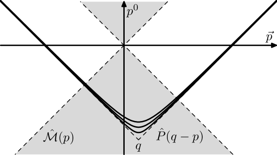
Figure 3. The convolution ${\hat{\mathcal{M}}}*\hat{P}$.

As a consequence, the convolution (B.3) is well-defined and finite if $q$ is chosen in the lower mass cone, because the integrand vanishes outside a bounded set (see Figure 3, where three Dirac seas are shown). However, if $q$ is chosen outside the lower mass cone, then the integration range in (B.3) is unbounded, and the integral will typically diverge. The assumption of a distributional ${\mathcal{M}}P$-product states that for $q$ in the lower mass cone, the distribution $\hat{Q}(q)$ (defined by (B.3) and removing the regularization) can be computed with this procedure.

Before going on, we point out that the assumption of a distributional ${\mathcal{M}}P$-product is not of fundamental significance. Instead, it is merely a simplifying assumption for the analysis of the causal action principle in the vacuum. At the time, it seemed appealing also because the geometric picture in Figure 3 seemed to give a simple explanation for the fact that in the vacuum the one-particle states of negative energy (and not the states of positive energy or the whole solution space) are occupied. A drawback of this assumption is that $\hat{Q}$ diverges in the upper mass cone. This means that, if one wants to recover the positive energy solutions of the Dirac equation as solutions of the linearized field equations (2.18), then the term $Q\,\delta\Psi$ diverges if the regularization is removed. In [18], this problem was bypassed by assuming that this divergence is compensated by the first summand $(DQ|_{\Psi}(\delta\Psi))\,\Psi$ in (2.18) (this leads to introducing the kernel $Q^{\text{dyn}}$; for details see [18, Sections 5.3 and 5.4]). However, as we will show below, a compensation of contributions between the first and second summand in (2.18) contradicts the approximate decoupling of the linearized field equations as worked out in Section 5. Therefore, the following considerations show that the assumption of a distributional ${\mathcal{M}}P$-product is too naive in the sense that it cannot hold for causal fermion systems describing our universe. As a consequence, some of the constructions in [18] are superseded by the constructions in the present paper. Moreover, we learn that those results in the papers [8, 13], where the assumption of a distributional ${\mathcal{M}}P$-product was used, need to be modified before they apply to physically realistic situations.

We now give the argument which rules out the assumption of a distributional ${\mathcal{M}}P$-product. Assume conversely that the assumption of a distributional ${\mathcal{M}}P$-product holds. Then, using that the integration range of the convolution in momentum space is compact (see Figure 3), the operator $\hat{Q}(k)$ is well-defined and finite inside the lower mass cone. Consequently, evaluating (2.17) for a state on the lower mass shell, one concludes that the parameter $\mathfrak{r}$ is also finite. However, $\hat{Q}(k)$ diverges inside the upper mass cone, with a singularity of the form (see [13])

$$\hat{Q}(k)\simeq\int\frac{m^{3}}{\xi^{4}}\>\not{\xi}\>P(x,y)\>d^{4}\xi\simeq\frac{m^{3}}{\varepsilon^{2}}$$ (B.4)

(here $\simeq$ means equality up to an irrelevant numerical constant). In order to make contact to relativistic quantum mechanics, the linearized field equations must admit solutions in the upper mass cone. Consequently, the left side of (5.5) has a singularity $\sim\varepsilon^{-2}$. The term on the right side of (5.5), however, diverges only $\sim\varepsilon^{-1}$, as we now explain. According to (5.6), we must consider the two contributions from (4.15) and (4.16). In (4.16) the Lagrange parameter $\kappa$ of the boundedness constraint appears. As shown in [3, Appendix A] it has the scaling

$$\kappa\lesssim(\varepsilon m)^{p}+\Big{(}\frac{\varepsilon}{\delta}\Big{)}^{8-\hat{s}}\>.$$

with $p\geq 4$ and $\hat{s}\in\{0,2\}$. Taking the Fourier transform gives a contribution with the scalings

$$\hat{Q}(k)\lesssim(\varepsilon m)^{4}\>\frac{1}{\varepsilon^{5}}=\frac{m^{4}}{\varepsilon}\>,$$

which differs from (B.4) by an additional factor $\varepsilon$, as desired.

It remains to consider the contribution (4.15). Here the first factor involves a scaling factor $\sim m^{3}$, because the eigenvalues have the same absolute values up to order ${\mathscr{O}}(m^{3})$. Next, we need to consider the two variational derivatives. One of them is used for testing; it appears similarly when varying (4.19). The second variational derivative, however, describes the linear perturbation of the system. The strength of this perturbation gives another scaling factor $\varepsilon/\ell_{\text{macro}}$ or $\varepsilon m$. Taking again the Fourier transform, we obtain the scaling

$$\hat{Q}(k)\lesssim(\varepsilon m)^{3}\>\frac{1}{\varepsilon^{5}}\>\Big{(}\varepsilon m+\frac{\varepsilon}{\ell_{\text{macro}}}\Big{)}\>.$$

This again differs from (B.4) by a scaling factor $\varepsilon$.

We conclude that the right side of (5.5) is by a scaling factor $\varepsilon$ smaller than the left side. This is a contradiction, showing that the assumption of a distributional $\mathcal{M}P$-product cannot hold.

Appendix C Regularity of $\hat{Q}$

In [22, Section 5.2] the commutator inner product was analyzed in Minkowski space. It was shown that it agrees with the usual scalar product on Dirac wave functions, up to a prefactor which is proportional to the discontinuity of the first derivative of $\hat{Q}(k)$, i.e. to the expression

$$\partial_{\omega}^{+}\hat{Q}(-\omega,\vec{k})-\partial_{\omega}^{-}\hat{Q}(-\omega,\vec{k})\>,$$ (C.1)

where $\omega:=\sqrt{|\vec{k}|^{2}-m^{2}}$, and the semi-derivatives are defined by

$$\partial_{\omega}^{+}\hat{Q}(-\omega,\vec{k}) =\lim_{h\searrow 0}\>\frac{1}{h}\,\Big{(}\hat{Q}(-\omega+h,\vec{k})-\hat{Q}(-\omega,\vec{k})\Big{)}$$

$$\partial_{\omega}^{-}\hat{Q}(-\omega,\vec{k}) =\lim_{h\nearrow 0}\>\frac{1}{h}\,\Big{(}\hat{Q}(-\omega+h,\vec{k})-\hat{Q}(-\omega,\vec{k})\Big{)}\>.$$

In view of this result, it is an important task to determine the regularity of $\hat{Q}$ and to verify whether this function can really have a discontinuity in its first derivative. We now analyze this question. We will find that $\hat{Q}\in C^{1}(\hat{M})$ is indeed continuously differentiable, showing that the expression (C.1) is zero. This also shows that the computation of the commutator inner product in [22, Section 5.2] is incomplete. This shortcoming is overcome by the construction in Section 6.3.

In general terms, the regularity of $\hat{Q}(k)$ in momentum space is related to decay properties of $Q(\xi)$ in position space. In order to see how this comes about, let us begin with the model example of a Lorentz invariant, complex-valued distribution of the form

$$U(x,y):=\int\frac{d^{4}p}{(2\pi)^{4}}\>f(p^{2})\>\Theta\big{(}-p^{2}\big{)}\>e^{-ip(x-y)}\>.$$ (C.2)

We consider the situation that for a parameter $a_{0}>0$, the function $f\in C^{0}_{0}(\mathbb{R}^{+})\cap C^{\infty}(\mathbb{R}^{+}\setminus\{a_{0}\})$ is piecewise smooth and vanishes at $p^{2}=a_{0}$ with a discontinuity of the first derivative, i.e.

$$\lim_{a\rightarrow a_{0},\;a\neq a_{0}}f(a)=0\qquad\text{and}\qquad c:=\lim_{a\searrow a_{0}}f^{\prime}(a)-\lim_{a\nearrow a_{0}}f^{\prime}(a)\neq 0\>.$$

Clearly, the distribution $U(x,y)$ depends only on the difference vector $\xi:=y-x$. The behavior of the function $U(x,y)$ for large $\xi$ could be analyzed in detail using methods of Fourier analysis. The result needed here can be seen most easily as follows. We first rewrite the kernel $U(x,y)$ as

$$U(x,y):=\int_{0}^{\infty}f(a)\>T_{a}(x,y)\>da\>,$$ (C.3)

where $T_{a}(x,y)$ is the Fourier transform of the lower mass shell,

$$T_{a}(x,y):=\int\frac{d^{4}p}{(2\pi)^{4}}\>\delta(p^{2}-a)\>\Theta\big{(}-p^{2}\big{)}\>e^{-ip(x-y)}\>.$$

This Fourier integral is a well-defined tempered distribution. It has a singular contribution on the light cone (i.e. if $(y-x)^{2}=0$), which is polynomial in $a$, so that the integral in (C.3) is well-defined, giving again a singular distribution on the light cone. Away from the light cone, however, $T_{a}(x,y)$ is a smooth function given by (see [10, eq. (1.2.29)])

$$T_{a}(x,y)=\left\{\begin{array}[]{cl}\displaystyle\frac{\sqrt{a}}{16\pi^{2}}\>\frac{Y_{1}\big{(}\sqrt{a\xi^{2}}\,\big{)}}{\sqrt{\xi^{2}}}+\frac{i\sqrt{m}}{16\pi^{2}}\>\frac{J_{1}\big{(}\sqrt{a\xi^{2}}\,\big{)}}{\sqrt{\xi^{2}}}\>\epsilon(\xi^{0})&\text{if~$\xi$ is timelike}\\[10.00002pt] \displaystyle\frac{\sqrt{a}}{8\pi^{3}}\frac{K_{1}\big{(}\sqrt{-a\xi^{2}}\,\big{)}}{\sqrt{-\xi^{2}}}&\text{if~$\xi$ is spacelike}\>,\end{array}\right.\hskip-3.00003pt$$

where $J_{1}$, $Y_{1}$ and $K_{1}$ are Bessel functions. For large values of their arguments, these Bessel functions have the asymptotics (see [28, eqs 10.7.8 and 10.25.3])

$$J_{1}(z) =\sqrt{\frac{2}{\pi z}}\>\cos\Big{(}z-\frac{\pi}{2}-\frac{\pi}{4}\Big{)}+{\mathscr{O}}\big{(}z^{-\frac{3}{2}}\big{)}$$

$$Y_{1}(z) =\sqrt{\frac{2}{\pi z}}\>\sin\Big{(}z-\frac{\pi}{2}-\frac{\pi}{4}\Big{)}+{\mathscr{O}}\big{(}z^{-\frac{3}{2}}\big{)}$$

$$K_{1}(z) =\sqrt{\frac{\pi}{2z}}\>e^{-z}\;\Big{(}1+{\mathscr{O}}\big{(}z^{-1}\big{)}\Big{)}\>.$$

Therefore, the function $T_{a}$ decays exponentially in spacelike directions, whereas for large timelike directions, it has the asymptotics

$$T_{a}(x,y)\simeq\frac{a^{\frac{1}{4}}}{\big{(}\xi^{2}\big{)}^{\frac{3}{4}}}\exp\Big{(}\pm i\sqrt{a\xi^{2}}\Big{)}\Big{(}1+{\mathscr{O}}\Big{(}\frac{1}{\sqrt{a\xi^{2}}}\Big{)}\Big{)}$$ (C.4)

(here $\simeq$ again means equality up to an irrelevant numerical constant). This formula holds similarly for derivatives of $T_{a}$, and the resulting formulas are obtained simply by differentiating the asymptotic formula. This makes it possible to determine the asymptotics of $U(x,y)$ with the following computation,

$$U(x,y) \simeq\frac{1}{\big{(}\xi^{2}\big{)}^{\frac{3}{4}}}\int_{0}^{\infty}a^{\frac{1}{4}}\>f(a)\>\exp\Big{(}\pm i\sqrt{a\xi^{2}}\Big{)}\>da\;\Big{(}1+{\mathscr{O}}\Big{(}\frac{1}{\sqrt{a\xi^{2}}}\Big{)}\Big{)}$$

$$\simeq\frac{1}{\big{(}\xi^{2}\big{)}^{\frac{3}{4}}}\int_{0}^{\infty}a^{\frac{1}{4}}\>f(a)\>\bigg{(}\frac{a}{\xi^{2}}\>\frac{d^{2}}{da^{2}}\exp\Big{(}\pm i\sqrt{a\xi^{2}}\Big{)}\bigg{)}\>da\;\Big{(}1+{\mathscr{O}}\Big{(}\frac{1}{\sqrt{a\xi^{2}}}\Big{)}\Big{)}$$

$$\simeq\frac{a_{0}^{\frac{1}{4}}}{\big{(}\xi^{2}\big{)}^{\frac{3}{4}}}\>\frac{a_{0}}{\xi^{2}}\>c\exp\Big{(}\pm i\sqrt{a_{0}\xi^{2}}\Big{)}\bigg{)}\>\Big{(}1+{\mathscr{O}}\Big{(}\frac{1}{\sqrt{a_{0}\xi^{2}}}\Big{)}\Big{)}\>,$$ (C.5)

where in the last step we integrated by parts twice and used that the boundary terms at $a=a_{0}$ arising from the discontinuity of the first derivative of $f$ give the leading contribution for large $a\xi^{2}$. Comparing with the asymptotics for $T_{a_{0}}$ in (C.4), we obtain the simple formula

$$U(x,y)\simeq\frac{a_{0}}{\xi^{2}}\>c\>T_{a_{0}}(x,y)\>\Big{(}1+{\mathscr{O}}\Big{(}\frac{1}{\sqrt{a_{0}\xi^{2}}}\Big{)}\Big{)}\>.$$ (C.6)

The next question is how Dirac matrices change the picture. To this end, we modify (C.2) by inserting a factor of $\not{p}$,

$$u(x,y):=\int\frac{d^{4}p}{(2\pi)^{4}}\>\not{p}\>f(p^{2})\>\Theta\big{(}-p^{2}\big{)}\>e^{-ip(x-y)}\>.$$ (C.7)

This factor can be rewritten with the Dirac operator which can be pulled out of the integral, i.e.

$$u(x,y)=i\mbox{$\partial$ \hskip-11.99998pt $/$}_{x}U(x,y)\>.$$

Consequently, differentiating (C.5) and comparing with the derivative of (C.4), we conclude that

$$u(x,y) \simeq\frac{a_{0}^{\frac{1}{4}}}{\big{(}\xi^{2}\big{)}^{\frac{3}{4}}}\>\frac{a_{0}}{\xi^{2}}\>c\>\big{(}\sqrt{a}\>\not{\xi}\big{)}\exp\Big{(}\pm i\sqrt{a_{0}\xi^{2}}\Big{)}\bigg{)}\>\Big{(}1+{\mathscr{O}}\Big{(}\frac{1}{\sqrt{a_{0}\xi^{2}}}\Big{)}\Big{)}$$

$$\simeq\frac{a_{0}}{\xi^{2}}\>(i\mbox{$\partial$ \hskip-11.99998pt $/$}_{x})T_{a}(x,y)\>.$$ (C.8)

Let us now analyze whether the asymptotics for large timelike $\xi$ found in either (C.6) and (C.8) can be found in the operator $Q(x,y)$. Thus let $\xi$ be a timelike vector. Since $P(x,y)$ is smooth at $\xi$, we may disregard the regularization. It then follows by direct computation that

$$P_{m}(x,y) =(i\mbox{$\partial$ \hskip-11.99998pt $/$}_{x}+m)\,T_{m^{2}}(x,y)$$

$$=\frac{m^{\frac{3}{2}}}{\big{(}\xi^{2}\big{)}^{\frac{3}{4}}}\Big{(}\mp\frac{\not{\xi}}{\sqrt{\xi^{2}}}+\mathds{1}\Big{)}\>\exp\Big{(}\pm im\sqrt{\xi^{2}}\Big{)}\Big{(}1+{\mathscr{O}}\Big{(}\frac{1}{\sqrt{\xi^{2}}}\Big{)}\Big{)}$$

$$\mathcal{M}_{xy} =P_{m}(x,y)\,P_{m}(y,x)-\frac{1}{4}\>\text{\rm{Tr}}\big{(}P_{m}(x,y)\,P_{m}(y,x)\big{)}$$

$$\simeq\frac{m^{3}}{\big{(}\xi^{2}\big{)}^{\frac{3}{2}}}\>\frac{\not{\xi}}{\sqrt{\xi^{2}}}+{\mathscr{O}}\big{(}\xi^{-4}\big{)}$$

$$Q(x,y) =\mathcal{M}_{xy}\,P_{m}(x,y)$$

$$\simeq\frac{m^{3}}{\big{(}\xi^{2}\big{)}^{\frac{3}{2}}}\>\frac{\not{\xi}}{\sqrt{\xi^{2}}}\>\frac{m^{\frac{3}{2}}}{\big{(}\xi^{2}\big{)}^{\frac{3}{4}}}\Big{(}\mp\frac{\not{\xi}}{\sqrt{\xi^{2}}}+\mathds{1}\Big{)}\>\exp\Big{(}\pm im\sqrt{\xi^{2}}\Big{)}\Big{(}1+{\mathscr{O}}\Big{(}\frac{1}{\sqrt{\xi^{2}}}\Big{)}\Big{)}$$

$$\simeq\frac{m^{3}}{\big{(}\xi^{2}\big{)}^{\frac{3}{2}}}\>P_{m}(x,y)\>\Big{(}1+{\mathscr{O}}\Big{(}\frac{1}{\sqrt{\xi^{2}}}\Big{)}\Big{)}\>.$$

The main conclusion is that, in contrast to the prefactor $1/\xi^{2}$ in (C.6) and (C.8), now a factor $(\xi^{2})^{-\frac{3}{2}}$ appears. Therefore, the kernel $Q(x,y)$ decays faster at infinity, meaning that its Fourier transform $\hat{Q}$ is more regular than the integrands in (C.2) and (C.7). We conclude that the discontinuity of the first derivatives in $\hat{Q}$ in (C.1) necessarily vanishes.

Here for simplicity we considered only one Dirac sea of mass $m$. Considering several Dirac seas, one also gets cross terms involving products of different masses. However, a direct computation shows that the scaling factor $(\xi^{2})^{-\frac{3}{2}}$ remains unchanged. Therefore, the function $\hat{Q}$ is again differentiable on the mass hyperbolas.

Appendix D What Causal Propagation Speed Means for the Structure of $\hat{Q}$

Let us assume that, after removing the regularization, $\hat{Q}(p)$ is a well-defined, Lorentz invariant distribution. Assuming vector-scalar structure, we can write it in the form

$$\hat{Q}(p)=f(p)\,\not{p}+g(p)$$ (D.1)

where $f$ and $g$ are Lorentz invariant, real-valued functions. The positivity statement of Proposition 3.2 implies that

$$\left\{\begin{array}[]{rl}f\sqrt{p^{2}}\geq|g|&\text{inside the upper mass cone}\\[3.00003pt] -f\sqrt{p^{2}}\geq|g|&\text{inside the lower mass cone}\>.\end{array}\right.$$

Outside the mass cone (i.e. if $p^{2}<0$), the ansatz (D.1) is compatible with positivity only if both $f$ and $g$ vanish. We conclude that $\hat{Q}$ can be written as

$$\hat{Q}(p)=\epsilon(p^{0})\>\Theta(p^{2})\>\times\left\{\begin{array}[]{cl}f^{\vee}(p^{2})\,\not{p}+g^{\vee}(p^{2})&\text{if~$p\in\mathcal{C}^{\vee}$}\\[3.00003pt] f^{\wedge}(p^{2})\,\not{p}+g^{\wedge}(p^{2})&\text{if~$p\in\mathcal{C}^{\wedge}$}\>,\end{array}\right.$$ (D.2)

where

$$f^{\vee}\geq\big{|}g^{\vee}\big{|}\qquad\text{and}\qquad f^{\wedge}\geq\big{|}g^{\wedge}\big{|}$$

(and $\mathcal{C}^{\vee}$ and $\mathcal{C}^{\wedge}$ denote the upper respectively lower mass cone).

We now introduce the corresponding symmetric Green’s operator as a distribution $\hat{S}(p)$ with the properties

$$\hat{S}(p)^{*}=\hat{S}(p)\qquad\text{and}\qquad\hat{Q}(p)\,\hat{S}(p)=\mathds{1}\quad\text{for all~$p\in{\mathcal{C}}$}\>.$$

This distribution can be introduced by treating poles in the familiar way as principal value integrals and distributional derivatives thereof. Further restrictions on the form of $\hat{S}$ are obtained by demanding causal propagation speed. This is not a new physical input but is a consequence of the general structure of the causal action principle. Moreover, causal propagation speed has been proven under general assumptions using energy methods in [4, 18]. In the setting considered here, causal propagation speed means that the distributional Fourier transform of $\hat{S}$ denoted by

$$S(x,y):=\int\frac{d^{4}p}{(2\pi)^{4}}\>\hat{S}(p)\>e^{-ip(x-y)}$$

must vanish if the difference vector $y-x$ is spacelike. This is indeed the case for symmetry reasons if

$$f^{\vee}=f^{\wedge}\qquad\text{and}\qquad g^{\vee}=g^{\wedge}\>.$$ (D.3)

The converse of this statement also holds under weak regularity and decay assumptions assumptions.

Lemma D.1.

Assume that the distribution $f:=f^{\vee}-f^{\wedge}\in\mathscr{D}^{\prime}(\mathbb{R}^{+}_{0})$ has the following properties:

• It is regular and locally bounded except at a finite number of singular points.

• It grows at most polynomially at $a=0$ and $a=\infty$.

Then the following implication holds: If the condition (D.3) is violated, then there is a spacelike vector $\xi=y-x$ such that $S(x,y)\neq 0$.

Proof.

Clearly, the distribution $\hat{S}(p)$ is again Lorentz invariant. We write it in analogy to (D.2) as

$$\hat{S}(p)=\epsilon(p^{0})\>\Theta(p^{2})\>\times\left\{\begin{array}[]{cl}\alpha^{\vee}(p^{2})\,\not{p}+\beta^{\vee}(p^{2})&\text{if~$p\in\mathcal{C}^{\vee}$}\\[3.00003pt] \alpha^{\wedge}(p^{2})\,\not{p}+\beta^{\wedge}(p^{2})&\text{if~$p\in\mathcal{C}^{\wedge}$}\>,\end{array}\right.$$

with suitable distributions $\alpha^{\bullet}$ and $\beta^{\bullet}$ (which could have poles, as described above). Its Fourier transform can be written as

$$S(x,y) =\frac{1}{2}\int_{0}^{\infty}\bigg{(}\big{(}\alpha^{\vee}-\alpha^{\wedge}\big{)}(a)\>i\mbox{$\partial$ \hskip-11.99998pt $/$}_{x}P_{a}(x,y)+\big{(}\alpha^{\vee}+\alpha^{\wedge}\big{)}(a)\>i\mbox{$\partial$ \hskip-11.99998pt $/$}_{x}K_{a}(x,y)\bigg{)}\>da$$

$$\quad\>+\frac{1}{2}\int_{0}^{\infty}\bigg{(}\big{(}\beta^{\vee}-\beta^{\wedge}\big{)}(a)\>P_{a}(x,y)+\big{(}\beta^{\vee}+\beta^{\wedge}\big{)}(a)\>K_{a}(x,y)\bigg{)}\>da\>,$$

where $P_{a}$ and $K_{a}$ are the symmetric and anti-symmetric fundamental solutions of the Klein-Gordon equation

$$P_{a}(x,y) :=\int\frac{d^{4}p}{(2\pi)^{4}}\>\delta(p^{2}-a)\>e^{-ip(x-y)}$$

$$K_{a}(x,y) :=\int\frac{d^{4}p}{(2\pi)^{4}}\>\delta(p^{2}-a)\>\epsilon(p^{0})\>e^{-ip(x-y)}\>.$$

Now suppose that $\xi$ is spacelike. Then the anti-symmetric fundamental solution $K_{a}$ vanishes. Expressing the symmetric fundamental solution in position space in terms of the Bessel function $K_{1}$,

$$P_{a}(x,y)=-\frac{a}{4\pi^{3}}\>\frac{K_{1}(\sqrt{-a\xi^{2}})}{\sqrt{-a\xi^{2}}}$$

(for details see for example [10, §1.2.5]), we obtain

$$S(x,y) =-\frac{i}{8\pi^{3}}\>(i\mbox{$\partial$ \hskip-11.99998pt $/$}_{x})\int_{0}^{\infty}\big{(}\alpha^{\vee}-\alpha^{\wedge}\big{)}(a)\>a\>\frac{K_{1}(\sqrt{-a\xi^{2}})}{\sqrt{-a\xi^{2}}}\>da$$

$$\quad\>-\frac{i}{8\pi^{3}}\>\int_{0}^{\infty}\big{(}\beta^{\vee}-\beta^{\wedge}\big{)}(a)\>a\>\frac{K_{1}(\sqrt{-a\xi^{2}})}{\sqrt{-a\xi^{2}}}\>da$$

$$=-\frac{i}{4\pi^{3}}\>(i\mbox{$\partial$ \hskip-11.99998pt $/$}_{x})\int_{0}^{\infty}\big{(}\alpha^{\vee}-\alpha^{\wedge}\big{)}\big{(}m^{2}\big{)}\>m^{2}\>\frac{K_{1}(m\sqrt{-\xi^{2}})}{\sqrt{-\xi^{2}}}\>dm$$

$$\quad\>-\frac{i}{4\pi^{3}}\>\int_{0}^{\infty}\big{(}\beta^{\vee}-\beta^{\wedge}\big{)}\big{(}m^{2}\big{)}\>m^{2}\>\frac{K_{1}(m\sqrt{-\xi^{2}})}{\sqrt{-\xi^{2}}}\>dm\>,$$

where $K_{1}$ is a modified Bessel function. In order to conclude that $\alpha^{\vee}=\alpha^{\wedge}$ and $\beta^{\vee}=\beta^{\wedge}$, one could argue with the invertibility of the Bessel or Mellin transformations (as considered in the related paper [29]). In order to weaken the regularity and decay assumptions, we prefer to apply Lemma D.2 below. We conclude that $S$ vanishes in spacelike directions if and only if $\alpha^{\vee}=\alpha^{\wedge}$ and $\beta^{\vee}=\beta^{\wedge}$. Taking the Fourier transformation, we obtain the corresponding symmetry property in position space (D.3). ∎

Lemma D.2.

Assume that $f\in\mathscr{D}^{\prime}(\mathbb{R}^{+}_{0})$ is a distribution having the properties (i) and (ii) in Lemma D.1. Moreover, assume that the distributional integral

$$g(\xi):=\int_{0}^{\infty}f(a)\>\frac{K_{1}(\sqrt{-a\xi^{2}})}{\sqrt{-\xi^{2}}}\>da\>.$$

vanishes for all spacelike $\xi$. Then $f$ is zero.

Proof.

Given any $p\in\mathbb{N}$, we consider the integral

$$0=\int_{\mathbb{R}^{3}}\bigg{|}\Big{(}\frac{\partial}{\partial\xi^{0}}\Big{)}^{p}g(\xi)\Big{|}_{\xi^{0}=0}\bigg{|}^{2}\>d^{3}\xi\>.$$

Applying Plancherel, it follows that

$$0=\int_{\mathbb{R}^{3}}\big{|}\hat{g}(\vec{k})\big{|}^{2}\>d^{3}k\>,$$

where

$$\hat{g}(\vec{k}):=\int_{0}^{\infty}da\>f(a)\int_{-\infty}^{\infty}d\omega\>\omega^{p}\>\delta\big{(}\omega^{2}-|\vec{k}|^{2}-a\big{)}=\int_{0}^{\infty}\big{(}|\vec{k}|^{2}+a\big{)}^{\frac{p-1}{2}}\>f(a)\>da\>.$$

Therefore, the last integral vanishes for almost all $\vec{k}$ and $p\in\mathbb{N}$. Choosing $p$ odd and taking derivatives with respect to $\vec{k}$, we conclude that the distributional integrals

$$\int_{0}^{\infty}\frac{a^{p}}{(1+a)^{q}}\>f(a)\>da$$

are well-defined and vanish for all $p,q\in\mathbb{N}_{0}$. We choose a parameter $r\in\mathbb{N}$ and a polynomial ${\mathcal{P}}(a)$ which is non-zero except at the origin and the singular points in such a way that the distribution

$$g(a):=\frac{{\mathcal{P}}(a)}{(1+a)^{r}}\>f(a)$$ (D.4)

is a regular and bounded function and $\lim_{a\rightarrow 0,\infty}g(a)=0$.

We want to show that the function $g$ vanishes. To this end, it is useful to consider the compactification $X=[0,\infty]$ as a compact metric space. On this space, we introduce the finite measure

$$d\mu(a)=\frac{da}{(1+a)^{2}}\>.$$

and regard $g$ as a vector in the Hilbert space $L^{2}(X,d\mu)$. Assume that $g$ is non-zero. Using that the continuous functions on $X$ are dense in $L^{2}(X,d\mu)$, there is a function $h\in C^{0}(X,\mathbb{R})$ with the property that

$$\int_{0}^{\infty}\overline{h}\>g\>d\mu\neq 0\>.$$ (D.5)

We next consider the algebra generated by the family of functions

$$h_{p,q}(a)=\frac{a^{p}}{(1+a)^{q}}\qquad\text{with~$0\leq p\leq q$}\>.$$

These functions are all continuous on $X$ and separate points. Therefore, according to the Stone-Weierstraß theorem, there is a sequence $h_{n}$ in the algebra which converges uniformly to $\overline{g}$. Lebesgue’s dominated convergence theorem implies that

$$0=\int_{0}^{\infty}\overline{h_{n}(a)}\>g(a)\>d\mu(a)\longrightarrow\int_{0}^{\infty}\overline{h}\,g\>d\mu\>,$$

in contradiction to (D.5). This proves that the function $g$ in (D.4) is zero.

We conclude that the distribution $f$ is supported at a finite number of points,

$$\operatorname{supp}f\subset\{0,a_{1},\ldots,a_{N}\}\>.$$

If $f$ is non-zero, there is a polynomial ${\mathcal{P}}$ with the property that ${\mathcal{P}}f$ is a non-trivial multiple of the Dirac distribution supported at one of these singular points. On the other hand, the distributional integral

$$\int_{0}^{\infty}{\mathcal{P}}(a)\>f(a)\>da$$

vanishes, a contradiction. ∎

We conclude that causality implies that $\hat{Q}$ must be of the form

$$\hat{Q}(p)=\epsilon(p^{0})\>\Theta(p^{2})\>\big{(}f(p^{2})\,\not{p}+g(p^{2})\big{)}$$

In particular, the solution space of the dynamical wave equation is necessarily symmetric under reflections $p\rightarrow-p$. This means that, having solutions on the lower mass shell of mass $m$, there must also be solutions on the upper mass shell corresponding to the same mass $m$.

Appendix E Example: A Regularized Dirac Dynamics

From the perspective of partial differential equations (PDEs), it might seem unusual or even surprising that the dynamical wave equation is obtained by minimizing the causal action. In contrast, hyperbolic equations like the scalar wave equation or the Dirac equation are obtained typically by seeking for critical points of an action, whereas a minimization process (like minimizing the Dirichlet energy) typically gives rise to elliptic equations. In order to explain and clarify this point, we now consider an example of a positive action with the property that minimizing this action gives rise to EL equations being hyperbolic PDEs. This example has a similar analytic structure as the effective action of the dynamical wave equation (6.1), so much so that it can be regarded as the PDE analog of this action.

We consider the following action in Minkowski space,

$$S(\psi):=\int_{-\infty}^{\infty}dt\int_{-\infty}^{\infty}dt^{\prime}\int_{\mathbb{R}^{3}}\!\!\!d^{3}x\;\mbox{$\prec\!\!$ \nolinebreak}\big{(}(i\mbox{$\partial$ \hskip-11.99998pt $/$}-m)\psi\big{)}(t,\vec{x})\>|\>\gamma^{0}\>\eta(t-t^{\prime})\>\big{(}(i\mbox{$\partial$ \hskip-11.99998pt $/$}-m)\psi\big{)}(t^{\prime},\vec{x})\mbox{\nolinebreak$\succ$}\>.$$ (E.1)

Here $\eta\in C^{\infty}(\mathbb{R})$ is a symmetric cutoff function (i.e. $\eta(t)=\eta(-t)$). We assume that its Fourier transform $\hat{\eta}$ is strictly positive, i.e.

$$\hat{\eta}(\omega)>0\qquad\text{for all~$\omega\in\mathbb{R}$}\>.$$ (E.2)

As a concrete example, one may choose $\eta$ as a Gaussian,

$$\eta(\tau)=e^{-\tau^{2}\delta}\qquad\text{with}\qquad\delta>0\>.$$

Considering first variations with compact support in spacetime, a direct computation gives the corresponding EL equations

$$(i\mbox{$\partial$ \hskip-11.99998pt $/$}-m)\,\gamma^{0}\,(i\mbox{$\partial$ \hskip-11.99998pt $/$}-m)\psi=0\>.$$ (E.3)

Lemma E.1.

The general solution $\psi\in C^{\infty}_{\text{\rm{sc}}}(M,SM)$ of the EL equations (E.3) can be written as

$$\psi(t,\vec{x})=\psi_{1}^{D}(t,\vec{x})+t\>\psi_{2}^{D}(t,\vec{x})\>,$$ (E.4)

where $\psi_{1\!/\!2}^{\text{D}}$ are solutions of the Dirac equation,

$$(i\mbox{$\partial$ \hskip-11.99998pt $/$}-m)\,\psi_{1\!/\!2}^{D}=0\>.$$

Proof.

Taking the Fourier transform of (E.3), we obtain the algebraic equation

$$0 =\gamma^{0}\,(\not{k}-m)\,\gamma^{0}\,(\not{k}-m)\,\hat{\psi}(k)$$ (E.5)

$$=\gamma^{0}\,\big{\{}\not{k},\gamma^{0}\big{\}}\,(\not{k}-m)\,\hat{\psi}(k)+(\gamma^{0})^{2}\>(-\not{k}-m)\,(\not{k}-m)\,\hat{\psi}(k)$$ (E.6)

$$=2k^{0}\,\gamma^{0}\,\,(\not{k}-m)\,\hat{\psi}(k)-(k^{2}-m^{2})\,\hat{\psi}(k)$$ (E.7)

$$=\big{(}|k^{0}|^{2}+|\vec{k}|^{2}+m^{2}-2\,k^{0}\gamma^{0}\,\vec{k}\vec{\gamma}-2m\,k^{0}\gamma^{0}\big{)}\,\hat{\psi}(k)\>.$$ (E.8)

The calculation

$$\big{(}-2\,k^{0}\gamma^{0}\,\vec{k}\vec{\gamma}-2m\,k^{0}\gamma^{0}\big{)}^{2}=4\,|k^{0}|^{2}\>\big{(}\gamma^{0}\,\vec{k}\vec{\gamma}+m\gamma^{0}\big{)}^{2}=4\,|k^{0}|^{2}\>\big{(}|\vec{k}|^{2}+m^{2}\big{)}$$

shows that the matrix in (E.5) has the eigenvalues

$$|k^{0}|^{2}+|\vec{k}|^{2}+m^{2}\pm 2k_{0}\,\sqrt{|\vec{k}|^{2}+m^{2}}=\Big{(}|k^{0}|\pm\sqrt{|\vec{k}|^{2}+m^{2}}\Big{)}^{2}\>.$$

In particular, one sees that the eigenvalues vanish only on the mass shells. Moreover, the $k^{0}$-derivative of the matrix in (E.5) is singular also only on the mass shells, because

$$\frac{\partial}{\partial k^{0}}\gamma^{0}\,(\not{k}-m)\,\gamma^{0}\,(\not{k}-m)=2\gamma^{0}\,(\not{k}-m)\>.$$

Therefore, the only distributional solutions of (E.8) have the form

$$\hat{\psi}_{1}(k)\>\delta\big{(}k^{2}-m^{2}\big{)}\qquad\text{and}\qquad\frac{\partial}{\partial k^{0}}\Big{(}\hat{\psi}_{2}(k)\>\delta\big{(}k^{2}-m^{2}\big{)}\Big{)}\>.$$

Transforming back to position space gives the result. ∎

We next restrict the above action to wave functions $\psi\in C^{\infty}_{0}((-t_{\min},t_{\max})\times\mathbb{R}^{3})$ supported in a time strip. This means in particular that we are not allowed to insert the solutions (E.4) into the action. But we may introduce a smooth cutoff function $\theta$ and take the functions

$$\psi(t,\vec{x})=\theta(t)\>\big{(}\psi_{1}^{D}(t,\vec{x})+t\>\psi_{2}^{D}(t,\vec{x})\big{)}\qquad\text{with}\qquad\theta\in C^{\infty}_{0}\big{(}(-t_{\min},t_{\max})\big{)}\>.$$

In the next lemma we verify that our action is strictly positive on such wave functions.

Lemma E.2.

Let $\psi$ be a smooth solution of the EL equations (E.3) of the form (E.4) defined in all of Minkowski space. Then the action (E.1) takes the form

$$S\big{(}\theta\>(\psi_{1}^{D}+t\,\psi_{2}^{D})\big{)}=\int_{-\infty}^{\infty}dt\int_{-\infty}^{\infty}dt^{\prime}\int_{\mathbb{R}^{3}}\!\!\!d^{3}x$$

$$\times\mbox{$\prec\!\!$ \nolinebreak}\Big{(}\theta^{\prime}(t)(\psi_{1}^{D}+t\,\psi_{2}^{D})+\theta(t)\,\psi_{2}^{D}\Big{)}$$

$$\qquad\qquad\qquad\times\>|\>\gamma^{0}\>\eta(t-t^{\prime})\>\Big{(}\theta^{\prime}(t^{\prime})(\psi_{1}^{D}+t^{\prime}\,\psi_{2}^{D})+\theta(t^{\prime})\,\psi_{2}^{D}\Big{)}\mbox{\nolinebreak$\succ$}\>.$$ (E.9)

This is strictly positive unless $\psi$ vanishes.

Proof.

Noting that

$$(i\mbox{$\partial$ \hskip-11.99998pt $/$}-m)\,\Big{(}\theta(t)(\psi_{1}^{D}+t\,\psi_{2}^{D})\Big{)}=i\gamma^{0}\Big{(}\theta^{\prime}(t)(\psi_{1}^{D}+t\,\psi_{2}^{D})+\theta(t)\,\psi_{2}^{D}\Big{)}\>,$$

we obtain (E.9). The strict positivity statement follows immediately by taking the Fourier transform in time and using (E.2). ∎

Integrating by parts, the above action (E.1) can be written in the form (6.1) if we introduce the distributional kernel

$$Q(x,y)=(i\mbox{$\partial$ \hskip-11.99998pt $/$}_{x}-m)\,\gamma^{0}\,(-i\mbox{$\partial$ \hskip-11.99998pt $/$}_{y}-m)\,\Big{(}\eta(t-t^{\prime})\>\delta^{3}(\vec{x}-\vec{y})\Big{)}\>.$$ (E.10)

Now we can use (2.20) to introduce a corresponding conserved inner product.

Lemma E.3.

Let $\psi$ and $\phi$ be solutions of the EL equations (E.3). Then

$$\langle\psi|\phi\rangle^{t_{2}} =-\int_{M}d^{4}x\int_{M}d^{4}y\>\eta(t-t^{\prime})\>\Big{(}\delta(t-t_{2})+\delta(t^{\prime}-t_{2})\Big{)}\>\delta^{3}(\vec{y}-\vec{x})$$

$$\qquad\>\times\Big{(}\mbox{$\prec\!\!$ \nolinebreak}\psi(x)\>|\>(i\mbox{$\partial$ \hskip-11.99998pt $/$}_{y}-m)\phi(y)\mbox{\nolinebreak$\succ$}+\mbox{$\prec\!\!$ \nolinebreak}(i\mbox{$\partial$ \hskip-11.99998pt $/$}_{x}-m)\psi(x)\>|\>\phi(y)\mbox{\nolinebreak$\succ$}\Big{)}\>.$$

Proof.

For notational simplicity, we compute the commutator inner product at time zero, so that

$$\langle\psi|\phi\rangle^{\Omega}=-2i\int_{M}d^{4}x\int_{M}d^{4}y\>\Big{(}\Theta(-t)\,\Theta(t^{\prime})-\Theta(t)\,\Theta(-t^{\prime})\Big{)}\>\mbox{$\prec\!\!$ \nolinebreak}\psi(x)\>|\>Q(x,y)\,\phi(y)\mbox{\nolinebreak$\succ$}\>.$$

Inserting (E.10) and integrating by parts, we obtain

$$\langle\psi|\phi\rangle^{\Omega} =i\int_{M}d^{4}x\int_{M}d^{4}y\>\eta(t-t^{\prime})\>\delta^{3}(\vec{y}-\vec{x})$$

$$\quad\>\times\Big{(}\mbox{$\prec\!\!$ \nolinebreak}(i\mbox{$\partial$ \hskip-11.99998pt $/$}_{x}-m)\big{(}\Theta(-t)\,\psi(x)\big{)}\>|\>\gamma^{0}\,(i\mbox{$\partial$ \hskip-11.99998pt $/$}_{y}-m)\big{(}\Theta(t^{\prime})\,\phi(y)\big{)}\mbox{\nolinebreak$\succ$}$$

$$\qquad\qquad\;\>-\mbox{$\prec\!\!$ \nolinebreak}(i\mbox{$\partial$ \hskip-11.99998pt $/$}_{x}-m)\big{(}\Theta(t)\,\psi(x)\big{)}\>|\>\gamma^{0}\,(i\mbox{$\partial$ \hskip-11.99998pt $/$}_{y}-m)\big{(}\Theta(-t^{\prime})\,\phi(y)\big{)}\mbox{\nolinebreak$\succ$}\Big{)}$$

$$=i\int_{M}d^{4}x\int_{M}d^{4}y\>\eta(t-t^{\prime})\>\delta^{3}(\vec{y}-\vec{x})$$

$$\quad\>\times\Big{(}i\delta(t)\,\mbox{$\prec\!\!$ \nolinebreak}\psi(x)\big{)}\>|\>(i\mbox{$\partial$ \hskip-11.99998pt $/$}_{y}-m)\phi(y)\mbox{\nolinebreak$\succ$}$$

$$\qquad\quad+\Theta(-t)\>\mbox{$\prec\!\!$ \nolinebreak}(i\mbox{$\partial$ \hskip-11.99998pt $/$}_{x}-m)\psi(x)\>|\>\gamma^{0}\,(i\mbox{$\partial$ \hskip-11.99998pt $/$}_{y}-m)\big{(}\Theta(t^{\prime})\,\phi(y)\big{)}\mbox{\nolinebreak$\succ$}$$

$$\qquad\quad-\Theta(t)\>\mbox{$\prec\!\!$ \nolinebreak}(i\mbox{$\partial$ \hskip-11.99998pt $/$}_{x}-m)\psi(x)\>|\>\gamma^{0}\,(i\mbox{$\partial$ \hskip-11.99998pt $/$}_{y}-m)\big{(}\Theta(-t^{\prime})\,\phi(y)\big{)}\mbox{\nolinebreak$\succ$}\Big{)}\>.$$

Now we integrate the Dirac operator by parts from the right to the left and use the relation

$$\Big{(}\frac{d}{dt}+\frac{d}{dt^{\prime}}\Big{)}\eta(t-t^{\prime})=0$$

as well as the EL equations (E.3). This gives

$$\langle\psi|\phi\rangle^{\Omega}$$

$$=i\int_{M}d^{4}x\int_{M}d^{4}y\>\eta(t-t^{\prime})\>\delta^{3}(\vec{y}-\vec{x})\;\Big{(}i\delta(t)\,\mbox{$\prec\!\!$ \nolinebreak}\psi(x)\big{)}\>|\>(i\mbox{$\partial$ \hskip-11.99998pt $/$}_{y}-m)\phi(y)\mbox{\nolinebreak$\succ$}$$

$$\qquad\quad+i\delta(t)\>\mbox{$\prec\!\!$ \nolinebreak}(i\mbox{$\partial$ \hskip-11.99998pt $/$}_{x}-m)\psi(x)\>|\>\Theta(t^{\prime})\,\phi(y)\mbox{\nolinebreak$\succ$}+i\delta(t)\>\mbox{$\prec\!\!$ \nolinebreak}(i\mbox{$\partial$ \hskip-11.99998pt $/$}_{x}-m)\psi(x)\>|\>\Theta(-t^{\prime})\,\phi(y)\mbox{\nolinebreak$\succ$}\Big{)}$$

$$=i\int_{M}d^{4}x\int_{M}d^{4}y\>\eta(t-t^{\prime})\>\delta^{3}(\vec{y}-\vec{x})$$

$$\quad\>\times\Big{(}i\delta(t)\,\mbox{$\prec\!\!$ \nolinebreak}\psi(x)\big{)}\>|\>(i\mbox{$\partial$ \hskip-11.99998pt $/$}_{y}-m)\phi(y)\mbox{\nolinebreak$\succ$}+i\delta(t)\>\mbox{$\prec\!\!$ \nolinebreak}(i\mbox{$\partial$ \hskip-11.99998pt $/$}_{x}-m)\psi(x)\>|\>\phi(y)\mbox{\nolinebreak$\succ$}\Big{)}$$

$$=-\int_{M}d^{4}x\int_{M}d^{4}y\>\eta(t-t^{\prime})\>\delta(t)\>\delta^{3}(\vec{y}-\vec{x})$$

$$\qquad\>\times\Big{(}\mbox{$\prec\!\!$ \nolinebreak}\psi(x)\big{)}\>|\>(i\mbox{$\partial$ \hskip-11.99998pt $/$}_{y}-m)\phi(y)\mbox{\nolinebreak$\succ$}+\mbox{$\prec\!\!$ \nolinebreak}(i\mbox{$\partial$ \hskip-11.99998pt $/$}_{x}-m)\psi(x)\>|\>\phi(y)\mbox{\nolinebreak$\succ$}\Big{)}\>.$$

Clearly, the commutator inner product is invariant under complex conjugation and exchanging $\psi$ with $\phi$. Therefore, we may symmetrize the right side as well. This gives the result. ∎

Using the representation (E.4) of the solution, we obtain

$$\langle\psi|\phi\rangle^{t_{2}} =-\int_{M}d^{4}x\int_{M}d^{4}y\>\eta(t-t^{\prime})\>\Big{(}\delta(t-t_{2})+\delta(t^{\prime}-t_{2})\Big{)}\>\delta^{3}(\vec{y}-\vec{x})$$

$$\qquad\>\times\Big{(}\mbox{$\prec\!\!$ \nolinebreak}\psi(x)\>|\>i\gamma^{0}\phi_{2}^{D}(y)\mbox{\nolinebreak$\succ$}+\mbox{$\prec\!\!$ \nolinebreak}i\gamma^{0}\psi_{2}^{D}(x)\>|\>\phi(y)\mbox{\nolinebreak$\succ$}\Big{)}$$

$$=-i\int_{M}d^{4}x\int_{M}d^{4}y\>\eta(t-t^{\prime})\>\Big{(}\delta(t-t_{2})+\delta(t^{\prime}-t_{2})\Big{)}\>\delta^{3}(\vec{y}-\vec{x})$$

$$\qquad\>\times\Big{(}\mbox{$\prec\!\!$ \nolinebreak}\psi(x)\>|\>\gamma^{0}\phi_{2}^{D}(y)\mbox{\nolinebreak$\succ$}+\mbox{$\prec\!\!$ \nolinebreak}\psi_{2}^{D}(x)\>|\>\gamma^{0}\phi(y)\mbox{\nolinebreak$\succ$}\Big{)}$$

$$=-i\int_{M}d^{4}x\int_{M}d^{4}y\>\eta(t-t^{\prime})\>\Big{(}\delta(t-t_{2})+\delta(t^{\prime}-t_{2})\Big{)}\>\delta^{3}(\vec{y}-\vec{x})$$

$$\qquad\>\times\Big{(}\mbox{$\prec\!\!$ \nolinebreak}\psi_{1}^{D}(x)\>|\>\gamma^{0}\phi_{2}^{D}(y)\mbox{\nolinebreak$\succ$}+\mbox{$\prec\!\!$ \nolinebreak}\psi_{2}^{D}(x)\>|\>\gamma^{0}\phi_{1}^{D}(y)\mbox{\nolinebreak$\succ$}\Big{)}$$

$$=-i\big{(}(\psi_{1}^{D}\>|\>\eta*\phi_{2}^{D})+(\psi_{2}^{D}\>|\>\eta*\phi_{1}^{D})-(\eta*\psi_{1}^{D}\>|\>\phi_{2}^{D})+(\eta*\psi_{2}^{D}\>|\>\phi_{1}^{D})\big{)}\>,$$

where the star denotes convolution in time and $(.|.)$ is the usual $L^{2}$-scalar product on Dirac spinors. Noting that the convolution preserves the Dirac equation, this is conserved in time, as desired.

We finally discuss the above example and explain the similarities and differences to the dynamical wave equation. We point out that the matrix in (E.8) involves a bilinear contribution and thus does not have a vector-scalar structure, in contrast to the action of the dynamical wave equation (6.1) when computed in Minkowski space (for details see [18, 22]). This can be regarded as being a shortcoming of the ansatz (E.1). This shortcoming can be avoided by choosing more sophisticated ansätze. An additional feature which one can build in is that the action is Lorentz invariant except for the regularization effects. For brevity, here we shall not enter a discussion of the different alternative ansätze, but restrict attention to the simple ansatz (E.1).

The main motivation for the action (E.1) comes from the fact it is positive (see Lemma E.2), making it possible to minimize the action. Nevertheless, the resulting EL equations give rise to hyperbolic equations (see Lemma E.1). Just as explained for the dynamical wave equation in Section 6, the prize to pay is that the resulting conserved inner product is not positive definite (see Lemma E.3). Therefore, following the procedure in Section 6.3, in order to introduce a Hilbert space of solutions, one needs to choose a positive definite subspace of the whole solution space. This can be accomplished by choosing the subspace spanned by solutions of the form

$$\psi(t,\vec{x})=\psi^{D}(t,\vec{x})+i\lambda t\>\psi^{D}(t,\vec{x})$$

with $\psi^{D}$ a solution of the Dirac equation. Here $\lambda>0$ is a small parameter (similar to the perturbation parameter $\lambda$ in Section 6.3). Then, linearly in $\lambda$, the inner product in Lemma E.3 simplifies to

$$\langle\psi|\psi\rangle^{t_{2}} =-\int_{M}d^{4}x\int_{M}d^{4}y\>\eta(t-t^{\prime})\>\Big{(}\delta(t-t_{2})+\delta(t^{\prime}-t_{2})\Big{)}\>\delta^{3}(\vec{y}-\vec{x})$$

$$\qquad\qquad\qquad\qquad\qquad\qquad\>\times\mbox{$\prec\!\!$ \nolinebreak}\psi^{D}(x)\>|\>\gamma^{0}\psi^{D}(y)\mbox{\nolinebreak$\succ$}+{\mathscr{O}}\big{(}\lambda^{2}\big{)}\>.$$

This is positive, as desired. Indeed,taking for $\eta$ a Dirac sequence and passing to the limit, one recovers the usual scalar product on Dirac solutions.

References

- [1] Link to web platform on causal fermion systems: www.causal-fermion-system.com.
- [2] Y. Bernard and F. Finster, On the structure of minimizers of causal variational principles in the non-compact and equivariant settings, arXiv:1205.0403 [math-ph], Adv. Calc. Var. 7 (2014), no. 1, 27–57.
- [3] E. Curiel, F. Finster, and J.M. Isidro, Two-dimensional area and matter flux in the theory of causal fermion systems, arXiv:1910.06161 [math-ph], Internat. J. Modern Phys. D 29 (2020), 2050098.
- [4] C. Dappiaggi and F. Finster, Linearized fields for causal variational principles: Existence theory and causal structure, arXiv:1811.10587 [math-ph], Methods Appl. Anal. 27 (2020), no. 1, 1–56.
- [5] C. Dappiaggi, F. Finster, N. Kamran, and M. Reintjes, Holographic mixing and Fock space dynamics of causal fermion systems, arXiv:2410.18045 [math-ph] (2024).
- [6] C. Dappiaggi, F. Finster, U. Moschella, and C. Paganini, Causal fermion systems in de Sitter spacetime, in preparation.
- [7] F. Finster, The Principle of the Fermionic Projector, hep-th/0001048, hep-th/0202059, hep-th/0210121, AMS/IP Studies in Advanced Mathematics, vol. 35, American Mathematical Society, Providence, RI, 2006.
- [8] by same author, On the regularized fermionic projector of the vacuum, arXiv:math-ph/0612003, J. Math. Phys. 49 (2008), no. 3, 032304, 60.
- [9] by same author, Causal variational principles on measure spaces, arXiv:0811.2666 [math-ph], J. Reine Angew. Math. 646 (2010), 141–194.
- [10] by same author, The Continuum Limit of Causal Fermion Systems, arXiv:1605.04742 [math-ph], Fundamental Theories of Physics, vol. 186, Springer, 2016.
- [11] by same author, Positive functionals induced by minimizers of causal variational principles, arXiv:1708.07817 [math-ph], Vietnam J. Math. 47 (2019), 23–37.
- [12] by same author, Solving the linearized field equations of the causal action principle in Minkowski space, arXiv:2304.00965 [math-ph], Adv. Theor. Math. Phys. 27 (2023), no. 7, 2087–2217.
- [13] F. Finster and S. Hoch, An action principle for the masses of Dirac particles, arXiv:0712.0678 [math-ph], Adv. Theor. Math. Phys. 13 (2009), no. 6, 1653–1711.
- [14] F. Finster, M. Jokel, and C.F. Paganini, A mechanism of baryogenesis for causal fermion systems, arXiv:2111.05556 [gr-qc], Class. Quant. Gravity 39 (2022), no. 16, 165005, 50.
- [15] F. Finster, R. Jonsson, M. Lottner, A. Much, and S. Murro, Notions of fermionic entropies for causal fermion systems, arXiv:2408.01710 [math-ph], Math. Phys. Anal. Geom. 28 (2025), no. 7, 42 pp.
- [16] F. Finster and N. Kamran, Fermionic Fock spaces and quantum states for causal fermion systems, arXiv:2101.10793 [math-ph], Ann. Henri Poincaré 23 (2022), no. 4, 1359–1398.
- [17] by same author, A positive quasilocal mass for causal variational principles, arXiv:2310.07544 [math-ph], Calc. Var. 64 (2025), 91.
- [18] F. Finster, N. Kamran, and M. Oppio, The linear dynamics of wave functions in causal fermion systems, arXiv:2101.08673 [math-ph], J. Differential Equations 293 (2021), 115–187.
- [19] F. Finster, N. Kamran, and M. Reintjes, Entangled quantum states of causal fermion systems and unitary group integrals, arXiv:2207.13157 [math-ph], Adv. Theor. Math. Phys. 27 (2023), no. 5, 1463–1589.
- [20] F. Finster and S. Kindermann, A gauge fixing procedure for causal fermion systems, arXiv:1908.08445 [math-ph], J. Math. Phys. 61 (2020), no. 8, 082301.
- [21] F. Finster, S. Kindermann, and J.-H. Treude, Causal Fermion Systems: An Introduction to Fundamental Structures, Methods and Applications, arXiv:2411.06450 [math-ph], to appear in Cambridge Monographs on Mathematical Physics, Cambridge University Press, 2025.
- [22] F. Finster and J. Kleiner, Noether-like theorems for causal variational principles, arXiv:1506.09076 [math-ph], Calc. Var. Partial Differential Equations 55:35 (2016), no. 2, 41.
- [23] by same author, A class of conserved surface layer integrals for causal variational principles, arXiv:1801.08715 [math-ph], Calc. Var. Partial Differential Equations 58:38 (2019), no. 1, 34.
- [24] F. Finster and C. Langer, Causal variational principles in the -locally compact setting: Existence of minimizers, arXiv:2002.04412 [math-ph], Adv. Calc. Var. 15 (2022), no. 3, 551–575.
- [25] F. Finster and M. Lottner, Banach manifold structure and infinite-dimensional analysis for causal fermion systems, arXiv:2101.11908 [math-ph], Ann. Global Anal. Geom. 60 (2021), no. 2, 313–354.
- [26] F. Finster and C. Paganini, Incompatibility of frequency splitting and spatial localization: A quantitative analysis of Hegerfeldt’s theorem, arXiv:2005.10120 [math-ph], Ann. Henri Poincaré 24 (2023), no. 2, 413–467.
- [27] F. Finster and A. Platzer, A positive mass theorem for static causal fermion systems, arXiv:1912.12995 [math-ph], Adv. Theor. Math. Phys. 25 (2021), no. 7, 1735–1818.
- [28] F.W.J. Olver, D.W. Lozier, R.F. Boisvert, and C.W. Clark (eds.), Digital Library of Mathematical Functions, National Institute of Standards and Technology from http://dlmf.nist.gov/ (release date 2019-12-15), Washington, DC, 2010.
- [29] P.G. Rooney, On the and transformations, Canadian J. Math. 32 (1980), no. 5, 1021–1044.