Efficient Learning on Large Graphs using a Densifying Regularity Lemma

Abstract

Learning on large graphs presents significant challenges, with traditional Message Passing Neural Networks suffering from computational and memory costs scaling linearly with the number of edges. We introduce the Intersecting Block Graph (IBG), a low-rank factorization of large directed graphs based on combinations of intersecting bipartite components, each consisting of a pair of communities, for source and target nodes. By giving less weight to non-edges, we show how to efficiently approximate any graph, sparse or dense, by a dense IBG. Specifically, we prove a constructive version of the weak regularity lemma, showing that for any chosen accuracy, every graph, regardless of its size or sparsity, can be approximated by a dense IBG whose rank depends only on the accuracy. This dependence of the rank solely on the accuracy, and not on the sparsity level, is in contrast to previous forms of the weak regularity lemma. We present a graph neural network architecture operating on the IBG representation of the graph and demonstrating competitive performance on node classification, spatio-temporal graph analysis, and knowledge graph completion, while having memory and computational complexity linear in the number of nodes rather than edges.

1 Introduction

Graphs are a powerful representation for structured data, with applications spanning social networks Hamilton et al. (2017a); Zeng et al. (2019), biological systems (Hamilton et al., 2017b), traffic modeling (Li et al., 2018), and knowledge graphs Kok and Domingos (2007), to name a few. As graph sizes continue to grow in application, learning on such large-scale graphs presents unique computational and memory challenges. Traditional Message Passing Neural Networks (MPNNs), which form the backbone of most graph signal processing architectures, scale their computational and memory requirements linearly with the number of edges. This edge-dependence limits their scalability in some situations, e.g., when processing social networks that can typically have $10^{8}\sim 10^{9}$ nodes and $10^{2}\sim 10^{3}$ as many edges Rossi et al. (2020). In the worst case of dense graphs, the complexity is quadratic in the number of nodes.

Several strategies, called graph reduction methods, have been proposed to alleviate these challenges in previous works. These include graph sparsification, where a smaller graph is randomly sampled from the large graph (Hamilton et al., 2017a; Zeng et al., 2019; Chen et al., 2018); graph condensation, where a new small graph is created (Jin et al., 2022; Wang et al., 2024; Zheng et al., 2024), representing structures in the large graph; and graph coarsening, where sets of nodes are grouped into super nodes (Ying et al., 2018; Bianchi et al., 2020; Huang et al., 2021). However, with the exception of graph sparsification, graph reduction methods typically do not address the problem of processing a graph that is too large to fit at once in memory (e.g., on the GPU). For an extended section on related work, see Appendix˜A.

Recently, Finkelshtein et al. (2024) proposed using a low-rank approximation of the graph, called Intersecting Community Graph (ICG), instead of the graph itself, for processing the data. If the graph is too large to fit in memory, the ICG factorization can be computed using a sparsification method. When training a model on the ICG representation, the computational complexity is reduced from linear in the number of edges (as in message-passing methods) to linear in the number of nodes. However, ICG has a number of limitations. First, the ICG approximation quality degrades with the sparsity of the graph, making ICG appropriate mainly for graphs that are both large and dense, a combination of requirements not always encountered in practice. Secondly, ICGs can only approximate undirected graphs. In this paper, we propose a non-trivial extension of the ICG method, called Intersecting Blocks Graph (IBG), addressing the aforementioned limitaitons and more.

(a) A directed graph.

(b) Approximating 3-IBG

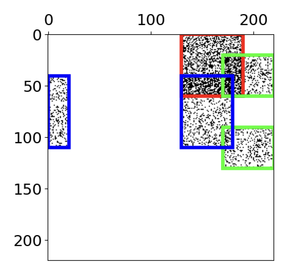
(c) The intersecting blocks of the 3-IBG.

Figure 1: (a) Directed graph sampled from a stochastic block model; (b) The approximating 3-IBG, where source and target community paris are represented by the same color; (c) Adjacency matrix of the 3-IBG shown as the intersecting blocks overlaid on the adjacency matrix. Here, we used a larger graph sampled from the same underlying stochastic block model.

Our contribution. We introduce a new procedure for approximating general directed graphs $G$ with adjacency matrices ${\bm{A}}\in\{0,1\}^{N\times N}$ by low-rank matrices ${\bm{C}}$ that have a special interpretation. The approximating graph consists of a set of overlapping bipartite components. Namely, there is a set of $K\ll N$ pairs of node communities $(\mathcal{U}_{i},\mathcal{V}_{i})$, $i=1,\ldots,K$, and each pair defines a weighted bipartite component, in which edges connect each node of $\mathcal{U}_{i}$ to each node of $\mathcal{V}_{i}$ with some weight $r_{i}$. The full graph ${\bm{C}}$ is defined to be the sum of all of these bipartite components, called blocks or directed communities, where the different communities can overlap. We demonstrate how processing ${\bm{C}}$ instead of ${\bm{A}}$ leads to models that solve downstream task in linear time and complexity with respect to the number of nodes, as opposed to standard message passing methods that are linear in the number of edges.

To fit ${\bm{C}}$ to ${\bm{A}}$, we consider a loss function $L_{{\bm{A}}}({\bm{C}})$ defined as a weighted norm of ${\bm{A}}-{\bm{C}}$, namely, a standard norm weighted element-wise by a weight matrix ${\bm{Q}}\in(0,\infty)^{N\times N}$. The goal of using weights is to balance the contributions of edges and non-edges. For this purpose, the weight matrix ${\bm{Q}}$ is chosen adaptively, i.e., it depends on the target adjacency matrix ${\bm{A}}$.

We consider a weighted cut norm, denoted by $\sigma_{\square}({\bm{A}}||{\bm{C}})$, as the approximation metric. The cut norm is a well-established graph similarity measure with a probabilistic interpretation that we discuss in Section˜3, Appendix˜B and C. Computing the cut norm is NP-hard, which prohibits explicitly optimizing it. To solve this issue, we prove that it is possible to minimize a weighted Frobenius norm $\left\|{\bm{A}}-{\bm{C}}\right\|_{\rm F}$ instead of the cut norm, and guarantee that the minimizer ${\bm{C}}^{*}$ has a small error $\sigma_{\square}({\bm{A}}||{\bm{C}}^{*})$, even if the minimum $\left\|{\bm{A}}-{\bm{C}}^{*}\right\|_{\rm F}$ is large. For that, we formulate a version of the Weak Regularity Lemma (WRL) (Frieze and Kannan, 1999) that we call the semi-constructive densifying directional soft weak regularity lemma, or in short the Densifying Weak Regularity Lemma.

The WRL asserts that one can approximate any graph with $E$ edges and $N$ nodes up to error $\epsilon$ w.r.t. the cut metric by a low-rank graph consisting of $N/(\sqrt{E}\epsilon^{2})$ intersecting communities. For more details on the standard WRL see Appendix˜B. Our approach, which is an extension of the IBG method (Finkelshtein et al., 2024), is different from other forms of the WRL in a number of ways outlined below.

• While some variants of the WRL only prove existence (László Miklós Lovász, 2007), we find the approximating low-rank graph as the solution to an “easy to optimize” loss function (hence our approach is constructive).

• While some versions of the WRL Frieze and Kannan (1999) propose an algorithm that provably obtains the approximating low-rank matrix, these algorithms are exponentially slow and not applicable in practice (for example, see the discussion in Section 7 of (Finkelshtein et al., 2024)). Instead, the loss function we introduce can be efficiently optimized via gradient descent. While the optimization procedure is not guaranteed to find the global minimum since the loss is non-convex, it nevertheless produces high-quality approximations in practice (hence the term semi-constructive). To facilitate a gradient descent-based optimization, we relax the combinatorial problem (hence the term soft).

• Previous versions of the WRL consider undirected graphs, while we treat general directed graphs (hence the term directional).

• While previous versions of the WRL required $N/(\sqrt{E}\epsilon^{2})$ communities for $\epsilon$ error w.r.t. the standard cut metric, we guarantee an $\epsilon$ error in weighted cut metric with only $1/\epsilon^{2}$ communities. Hence, as opposed to past methods like Finkelshtein et al. (2024), the number of communities in our method is independent of any property of the graph, including the number of nodes and sparsity level. This capability directly follows the fact that we balance the importance of edges and non-edges in our optimization target, which effectively leads to a formal approach for approximating sparse large graphs by dense low rank graphs, justifying the term densifying in the name of our lemma. We emphasize that this independence of the number of communities on the sparsity level is not merely an artifact of carefully renormalizing the loss to artificially facilitate the desired error bound. Rather, the loss function is deliberately designed to promote denseness when approximating graphs. The ability to efficiently densify a given graph can improve downstream tasks like node classification, as, in some sense, the densified version ${\bm{C}}^{*}$ of the graph ${\bm{A}}$ strengthens the connectivity patterns of the graph, at the expense of damping the disconnection patterns, which typically carry less structural information in sparse graphs. We empirically demonstrate that densifying the graph improves the performance of graph machine learning tasks. We stress that as opposed to naive densification approaches, like 2-hop neighborhood graphs, densifying with our method improves both computational complexity and accuracy.

We call the approximating low-rank graph IBG. Given a graph, we construct a neural network, called IBG-NN, that directly processes that IBG approximation of the graph instead of the original graph itself. IBG-NN allow solving downstream tasks such as node classification, spatio-temporal graph analysis, and knowledge graph completion in ${\mathcal{O}}(N)$ operations rather than ${\mathcal{O}}(E)$. We demonstrate that such an approach achieves state-of-the art accuracy on standard benchmarks, while being very efficient. For background on the predecessor of our method, ICG Finkelshtein et al. (2024), see Appendix A. For a comparison of our method with ICG, see Section˜7.2 and Appendices˜J and L.4.

2 Basic definitions and notations

We denote matrices by boldface uppercase letters, e.g., ${\bm{D}}$, vectors by boldface lowercase ${\bm{d}}$, and their scalar entries by the same lowercase letter $d_{i}$ with subscript for the index.

Graph signals. We consider directed (unweighted) graphs $G$ with sets of $N$ nodes $\mathcal{V}=[N]=\{1,\dots,N\}$, $E$ edges ${\mathcal{E}}\subseteq\mathcal{V}\times\mathcal{V}$, adjacency matrix ${\bm{A}}=(a_{i,j})_{i,j=1}^{N}\in\{0,1\}^{N\times N}$, and node feature matrix ${\bm{X}}=(x_{i,j})_{i,j=1}^{N,D}\in[-1,1]^{N\times D}$, called the signal. We follow the graph signal processing convention and represent the data as graph-signals $G=({\bm{A}},{\bm{X}})$. We emphasize that signals are always normalized to have values in $[-1,1]$, which does not limit generality as the units of measurement can always be linearly changed. All constructions also apply to signals with values in ${\mathbb{R}}$, but for simplicity of the analysis we limit the values to $[-1,1]$.

We denote the $j$-th column of the matrix ${\bm{Q}}$ by ${\bm{Q}}_{:,j}$, and the $i$-th row by ${\bm{Q}}_{i,:}$. We often also denote the $i$-th row by ${\bm{q}}_{i}^{\top}$ and respectively denote ${\bm{Q}}=({\bm{q}}_{i})_{i=1}^{M}$. We identify vectors ${\bm{v}}=(v_{1})_{i=1}^{N}$ with corresponding functions $i\mapsto v_{i}$. Similarly, we treat ${\bm{X}}$ as a function ${\bm{X}}:[N]\to{\mathbb{R}}^{D}$, with ${\bm{X}}(n)={\bm{x}}_{n}$. We denote by $\operatorname{diag}({\bm{r}})\in{\mathbb{R}}^{K\times K}$ the diagonal matrix with diagonal elements ${\bm{r}}\in{\mathbb{R}}^{K}$. The pseudoinverse of a full-rank matrix ${\bm{W}}\in{\mathbb{R}}^{N\times K}$, where $N\geq K$, is ${\bm{W}}^{\dagger}=({\bm{W}}^{\top}{\bm{W}})^{-1}{\bm{W}}^{\top}$.

Frobenius norm. The weighted Frobenius norm of a square matrix ${\bm{D}}\in{\mathbb{R}}^{N\times N}$ with respect to the weight ${\bm{Q}}\in(0,\infty)^{N\times N}$ is defined to be $\left\|{\bm{D}}\right\|_{{\rm F};{\bm{Q}}}:=\sqrt{\frac{1}{\sum_{i,j=1}^{N}q_{i,j}}\sum_{i,j=1}^{N}d_{i,j}^{2}q_{i,j}}$. Denote $\left\|{\bm{D}}\right\|_{\rm F}:=\left\|{\bm{D}}\right\|_{\rm F;\mathbf{1}}$, where $\mathbf{1}$ is the all-1 matrix. The Frobenius norm of a signal ${\bm{Y}}\in{\mathbb{R}}^{N\times D}$ is defined by $\left\|{\bm{Y}}\right\|_{\rm F}:=\sqrt{\frac{1}{ND}\sum_{j=1}^{D}\sum_{i=1}^{N}y_{i,j}^{2}}$. The weighted Frobenius norm with weights $\alpha,\beta>0$ of a matrix-signal $({\bm{D}},{\bm{Y}})$, is defined to be $\left\|({\bm{D}},{\bm{Y}})\right\|_{{\rm F};{\bm{Q}}}=\left\|({\bm{D}},{\bm{Y}})\right\|_{{\rm F};{\bm{Q}},\alpha,\beta}:=\sqrt{\alpha\left\|{\bm{D}}\right\|_{{\rm F};{\bm{Q}}}^{2}+\beta\left\|{\bm{Y}}\right\|_{\rm F}^{2}}$.

3 Weighted graph similarity measures

Weighted cut-metric. The cut-metric is a graph similarity measure based on the cut-norm. Below, we define it for graphs of the same size; extensions to arbitrary graphs use graphons (see (László Miklós Lovász, 2007) for graphons, and (Levie, 2023) for graphon-signals).

Definition 3.1.

The weighted matrix cut-norm of ${\bm{D}}\in{\mathbb{R}}^{N\times N}$ with weights ${\bm{Q}}\in(0,\infty)^{N\times N}$, is defined to be

$$\left\|{\bm{D}}\right\|_{\square;{\bm{Q}}}=\frac{1}{\sum_{i,j}q_{i,j}}\max_{{\mathcal{U}},{\mathcal{V}}\subset[N]}\Big{|}\sum_{i\in{\mathcal{U}}}\sum_{j\in{\mathcal{V}}}d_{i,j}q_{i,j}\Big{|}.$$

The signal cut-norm of ${\bm{Y}}\in{\mathbb{R}}^{N\times D}$ is defined to be

$$\left\|{\bm{Y}}\right\|_{\square}=\frac{1}{DN}\sum_{j=1}^{D}\max_{{\mathcal{U}}\subset[N]}\Big{|}\sum_{i\in{\mathcal{U}}}y_{i,j}\Big{|}.$$

The weighted matrix-signal cut-norm of $({\bm{D}},{\bm{Y}})$, with weights $\alpha,\beta>0$, is defined to be

$$\begin{split}\left\|({\bm{D}},{\bm{Y}})\right\|_{\square;{\bm{Q}}}&=\left\|({\bm{D}},{\bm{Y}})\right\|_{\square;{\bm{Q}},\alpha,\beta}\\ &:=\alpha\left\|{\bm{D}}\right\|_{\square;{\bm{Q}}}+\beta\left\|{\bm{Y}}\right\|_{\square}.\end{split}$$ (1)

Note that Finkelshtein et al. (2024) uses a weighted matrix-signal cut-norm via $\left\|{\bm{D}}\right\|_{\square}:=(N^{2}/E)\left\|{\bm{D}}\right\|_{\square;\mathbf{1}}$.

The weighted cut-metric between two graphs ${\bm{A}}$ and ${\bm{A}}^{\prime}$ is defined to be the cut-norm of their difference $\left\|{\bm{A}}-{\bm{A}}^{\prime}\right\|_{\square;{\bm{A}}}$. This distance represents the maximum (weighted) discrepancy in edge densities of ${\bm{A}}$ and ${\bm{A}}^{\prime}$ across all blocks, giving the cut-metric a probabilistic interpretation. For simple graphs ${\bm{A}},{\bm{A}}^{\prime}$, the difference ${\bm{A}}-{\bm{A}}^{\prime}$ is a granular function with values jumping between $-1$, $0$, and $1$. In such a case $\ell_{p}$ norms of ${\bm{A}}-{\bm{A}}^{\prime}$ tend to be large. In contrast, the fact that the absolute value in (1) is outside the sum, unlike the $\ell_{1}$ norm, results in an averaging effect, which can lead to a small distance between ${\bm{A}}$ and ${\bm{A}}^{\prime}$ in the cut distance even if ${\bm{A}}-{\bm{A}}^{\prime}$ is granular.

Densifying cut similarity.

A key limitation of the cut-metric in sparse graphs arises from the dominance of non-edges in the graph structure. Sparse graphs, such as those encountered in link prediction and knowledge graph completion (Farzaneh et al., 2015; Dettmers et al., 2018), often have a small number of edges relative to non-edges. This imbalance causes non-edges to disproportionately influence the metric unless properly weighted.

We believe that this imbalance significantly impacted the quality of the approximating low-rank matrix (ICG) in Finkelshtein et al. (2024), which uses the unweighted cut-metric, i.e. with ${\bm{Q}}=\mathbf{1}$, and consequently the underperformance of downstream tasks which operate on the ICG representation.

Motivated by this limitation, we define a similarity measure that better addresses the structural imbalance inherent in sparse graphs. We propose the densifying cut similarity, a modification of the cut-metric that lowers the contributions of non-edges w.r.t. the standard cut-metric. The approach involves defining a weighted adjacency matrix ${\bm{Q}}$ that assigns a weight $e$ to non-edges and $1$ to edges. The parameter $e$ is chosen based on the desired balance, controlled by a factor $\Gamma$, which determines the proportion of non-edges relative to edges. For a detailed derivation of the definition from motivating guidelines, and its relation to negative sampling in knowledge graph completion and link prediction, see Appendix˜C.

Definition 3.2.

Let ${\bm{A}}\in\{0,1\}^{N\times N}$ be an unweighted adjacency matrix, and $\Gamma>0$. The densifying cut similarity between the target ${\bm{A}}$ and any adjacency matrix ${\bm{B}}\in\mathbb{R}^{N\times N}$ is defined to be

$$\sigma_{\square}({\bm{A}}||{\bm{B}})=\sigma_{\square;\Gamma}({\bm{A}}||{\bm{B}}):=(1+\Gamma)\left\|{\bm{A}}-{\bm{B}}\right\|_{\square;{\bm{Q}}_{{\bm{A}}}},$$

where the weight matrix ${\bm{Q}}_{\bm{A}}$ is

$${\bm{Q}}_{{\bm{A}}}={\bm{Q}}_{{\bm{A}},\Gamma}:=e_{E,\Gamma}\mathbf{1}+(1-e_{E,\Gamma}){\bm{A}},$$ (2)

with $e_{E,\Gamma}=\frac{\Gamma E/N^{2}}{1-(E/N^{2})}$.

Given $\alpha,\beta>0$ such that $\alpha+\beta=1$, the densifying cut similarity between the target graph-signal $({\bm{A}},{\bm{X}})$ and the graph-signal $({\bm{A}}^{\prime},{\bm{X}}^{\prime})$ is defined to be

$$\sigma_{\square}\big{(}({\bm{A}},{\bm{X}})||({\bm{A}}^{\prime},{\bm{X}}^{\prime})\big{)} =\sigma_{\square;\alpha,\beta,\Gamma}\big{(}({\bm{A}},{\bm{X}})||({\bm{A}}^{\prime},{\bm{X}}^{\prime})\big{)}$$

$$:=\alpha\sigma_{\square;\Gamma}({\bm{A}}||{\bm{B}})+\beta\left\|{\bm{X}}-{\bm{X}}^{\prime}\right\|_{\square}.$$

We stress that the weighted Frobenius norm with the weight from Definition 3.2 is well normalized, i.e., $(1+\Gamma)\left\|{\bm{A}}\right\|_{{\mathrm{F}};{\bm{Q}}_{{\bm{A}}}}=1$, suggesting that the norm $\sigma_{\square}\big{(}({\bm{A}},{\bm{X}})||({\bm{A}}^{\prime},{\bm{X}}^{\prime})\big{)}$ is meaningfully standardized. Namely, we expect $\sigma_{\square}\big{(}({\bm{A}},{\bm{X}})||({\bm{A}}^{\prime},{\bm{X}}^{\prime})\big{)}$ to have magnitude of the order of 1 when ${\bm{B}}$ is a “bad” approximation of ${\bm{A}}$, and to be $\ll 1$ when ${\bm{B}}$ is a “good” approximation.

4 Approximations by intersecting blocks

4.1 Intersecting block graphs

For any subset of nodes ${\mathcal{U}}\subset[N]$, the indicator function $\bm{\mathbbm{1}}_{{\mathcal{U}}}$ is defined as $\bm{\mathbbm{1}}_{{\mathcal{U}}}(i)=1$ if $i\in{\mathcal{U}}$ and $0$ otherwise. As explained above, we treat $\bm{\mathbbm{1}}_{{\mathcal{U}}}$ as a vector in ${\mathbb{R}}^{N}$. Denote by $\chi$ the set of all such indicator functions.

We define an Intersecting Block Graph (IBG) with $K$ classes ($K$-IBG) as a low-rank graph-signal $({\bm{C}},{\bm{P}})$ with adjacency matrix and signals given respectively by

$${\bm{C}}=\sum_{j=1}^{K}r_{j}\bm{\mathbbm{1}}_{{\mathcal{U}}_{j}}\bm{\mathbbm{1}}_{{\mathcal{V}}_{j}}^{\top},\quad{\bm{P}}=\sum_{j=1}^{K}\bm{\mathbbm{1}}_{{\mathcal{U}}_{j}}{\bm{f}}_{j}^{\top}+\bm{\mathbbm{1}}_{{\mathcal{V}}_{j}}{\bm{b}}_{j}^{\top}$$

where $r_{j}\in{\mathbb{R}}$, ${\bm{f}}_{j},{\bm{b}}_{j}\in{\mathbb{R}}^{D}$, and ${\mathcal{U}}_{j},{\mathcal{V}}_{j}\subset[N]$. Next, we relax the $\{0,1\}$-valued hard indicator functions $\bm{\mathbbm{1}}_{{\mathcal{U}}},\bm{\mathbbm{1}}_{{\mathcal{V}}}$ to soft affiliation functions with values in ${\mathbb{R}}$, as defined next, to allow continuously optimizing IBGs. The following definition is taken from Finkelshtein et al. (2024).

Definition 4.1.

A set ${\mathcal{Q}}$ of functions ${\bm{u}}:[N]\rightarrow{\mathbb{R}}$ (namely vectors) that contains $\chi$ is called a soft affiliation model.

The following definition extends Finkelshtein et al. (2024) to directed graphs with signals.

Definition 4.2.

Let $d\in\mathbb{N}$, and let ${\mathcal{Q}}$ be a soft affiliation model. We define $[{\mathcal{Q}}]\subset\mathbb{R}^{N\times N}\times\mathbb{R}^{N\times D}$ to be the set of all elements of the form $(r{\bm{u}}{\bm{v}}^{\top},{\bm{u}}{\bm{f}}^{\top}+{\bm{v}}{\bm{b}}^{\top})$, with ${\bm{u}},{\bm{v}}\in{\mathcal{Q}}$, $r\in{\mathbb{R}}$ and ${\bm{f}},{\bm{b}}\in{\mathbb{R}}^{D}$. We call $[{\mathcal{Q}}]$ the soft rank-1 intersecting block graph (IBG) model corresponding to ${\mathcal{Q}}$. Given $K\in{\mathbb{N}}$, the subset $[{\mathcal{Q}}]_{K}$ of ${\mathbb{R}}^{N\times N}\times{\mathbb{R}}^{N\times D}$ of all linear combinations of $K$ elements of $[{\mathcal{Q}}]$ is called the soft rank-$K$ IBG model corresponding to ${\mathcal{Q}}$.

In matrix form, an IBG $({\bm{C}},{\bm{P}})\in{\mathbb{R}}^{N\times N}\times{\mathbb{R}}^{N\times D}$ in $[{\mathcal{Q}}]_{K}$ can be written as

$${\bm{C}}={\bm{U}}\operatorname{diag}({\bm{r}}){\bm{V}}^{\top}\quad\text{and}\quad{\bm{P}}={\bm{U}}{\bm{F}}+{\bm{V}}{\bm{B}}$$ (3)

via the target community affiliation matrix ${\bm{U}}\in{\mathbb{R}}^{N\times K}$, the source community affiliation matrix ${\bm{V}}\in{\mathbb{R}}^{N\times K}$, the community magnitude vector ${\bm{r}}\in{\mathbb{R}}^{K}$, the target community feature matrix ${\bm{F}}\in{\mathbb{R}}^{K\times D}$ and the source community feature matrix ${\bm{B}}\in{\mathbb{R}}^{K\times D}$.

4.2 The densifying regularity lemma

Directly minimizing the densifying cut similarity (or even the cut metric) is both numerically unstable and computationally difficult to solve since it involves a maximization step, making the optimization a min-max problem. While Frieze and Kannan (1999) proposed an algorithm that provably addresses this issue, it comes with the significant drawback of an impractical runtime $Ne^{{\mathcal{O}}(K)}$. To overcome this, we introduce a middle-ground solution, which extends the semi-constructive regularity lemma of Finkelshtein et al. (2024), providing an efficient semi-constructive version of the weak regularity lemma for intersecting blocks.

This approach is termed semi-constructive because it formulates the approximating graph as the solution to an "easy-to-solve" optimization problem that can be efficiently handled using standard gradient descent techniques. In Theorem˜4.1, we prove that, with high probability, one can achieve a small densifying cut similarity error by minimizing the weighted Frobenius norm error, allowing us to replace the original untractable densifying cut similarity with the stable and computationally tractable weighted Frobenius error. While the problem remains non-convex and thus lacks guarantees for convergence to a global minimum, empirical evidence strongly supports the effectiveness of a gradient-based approach for minimizing the Frobenius norm (see Section˜5).

The theorem generalizes the semi-constructive WRL based on intersecting communities of Finkelshtein et al. (2024) in three main ways: (1) extending the theorem to directed graphs, (2) introducing a certificate for testing that the high probability event in which the cut similarity error is small occurred, and the key novelty of this theorem – (3) it addresses a major limitation of the previous work by providing a bound that is independent of the graph size for both sparse and dense graphs, whereas the bound in Finkelshtein et al. (2024) depended on the graph size for sparse graphs. For a comparison between our approach and Finkelshtein et al. (2024) see Appendix J.

Theorem 4.1.

Let $({\bm{A}},{\bm{S}})$ be a graph-signal, $K\in\mathbb{N}$, $\delta>0$, and let $\mathcal{Q}$ be a soft indicators model. Let $\alpha,\beta>0$ such that $\alpha+\beta=1$. Let $\Gamma>0$ and let ${\bm{Q}}_{{\bm{A}}}$ be the weight matrix defined in Definition˜3.2. Let $R\geq 1$ such that $K/R\in\mathbb{N}$. For every $k\in\mathbb{N}$, let

$$\eta_{k}=(1+\delta)\min_{({\bm{C}},{\bm{P}})\in[\mathcal{Q}]_{k}}\left\|({\bm{A}},{\bm{S}})-({\bm{C}},{\bm{P}})\right\|^{2}_{{\rm F};{\bm{Q}}_{{\bm{A}}},\alpha(1+\Gamma),\beta}$$

Then,

1. For every $m\in\mathbb{N}$, any IBG $({\bm{C}}^{*},{\bm{P}}^{*})\in[\mathcal{Q}]_{m}$ that gives a close-to-best weighted Frobenius approximation of $({\bm{A}},{\bm{S}})$ in the sense that

   $$\left\|({\bm{A}},{\bm{S}})-({\bm{C}}^{*},{\bm{P}}^{*})\right\|^{2}_{{\rm F};{\bm{Q}}_{{\bm{A}}},\alpha(1+\Gamma),\beta}\leq\eta_{m},$$ (4)

   also satisfies

   $$\sigma_{\square;\alpha,\beta,\Gamma}\big{(}({\bm{A}},{\bm{S}})||({\bm{C}}^{*},{\bm{P}}^{*})\big{)}\leq(\sqrt{\alpha(1+\Gamma)}+\sqrt{\beta})\sqrt{\eta_{m}-\frac{\eta_{m+1}}{1+\delta}}.$$ (5)

2. If $m$ is uniformly randomly sampled from $[K]$, then in probability $1-\frac{1}{R}$ (with respect to the choice of $m$),

   $$\sqrt{\eta_{m}-\frac{\eta_{m+1}}{1+\delta}}\leq\sqrt{\frac{\delta}{1+\delta}+\frac{R(1+\delta)}{K}}$$ (6)

   Specifically, in probability $1-\frac{1}{R}$, any $({\bm{C}}^{*},{\bm{P}}^{*})\in[\mathcal{Q}]_{m}$ which satisfies (4), also satisfies

   $$\sigma_{\square,\alpha,\beta}\big{(}({\bm{A}},{\bm{X}})-({\bm{C}}^{*},{\bm{P}}^{*})\big{)}\leq\sqrt{2+\Gamma}\sqrt{\frac{\delta}{1+\delta}+\frac{R(1+\delta)}{K}}.$$ (7)

The proof of Theorem 4.1 is in Appendix D.

4.3 Optimizing IBGs with oracle Frobenius minimizers

Theorem˜4.1 motivates the following algorithm for approximating a graph-signal by an IBG. Suppose there exists an oracle optimization method that solves (4) in $T_{K}$ operations for any $m\leq K$. The algorithm proceeds as follows.

• Randomly sample $m\in[K]$. By Item˜2 of Theorem˜4.1, the approximation bound (7) is satisfied in high probability $(1-1/R)$.

• To verify that (7) really happened for the given realization of $m$, we estimate the left-hand-side of (6), using the oracle optimizer in $2T_{K}$ operations (computing both $\eta_{m}$ and $\eta_{m+1}$), checking if (6) is satisfied. If it is, it guarantees (7) by (5).

• If the bound (6) is not satisfied (in probability less than $\frac{1}{R}$), resample $m$ and repeat.

The expected number of resamplings of $m$ is $R/(R-1)$, so the algorithm’s expected runtime to find an IBG satisfying (7) is $2T_{K}R/(R-1)$. In practice, instead of an oracle optimizer, we apply gradient descent to estimate the optimum of the left-hand side of (4), which requires $T_{K}={\mathcal{O}}(E)$ operations as established in Proposition˜5.1. This makes the algorithm as efficient as message passing in practice.

4.4 The learning pipeline with IBGs

When learning on large graphs using IBGs, the first step in the pipeline is fitting an IBG to the given graph. This is done once with little to no hyperparameter tuning in ${\mathcal{O}}(E)$ time and memory complexity. The second step of the pipeline is solving the task on the graph, e.g., node classification, or spatio-temporal prediction. This step typically involves an extensive architecture and hyperparameter search. In our pipleline, the neural network processes the efficient IBG representation of the data, instead of processing directly the standard representation of the graph. This improves the processing time and memory complexity from ${\mathcal{O}}(E)$ to ${\mathcal{O}}(N)$, as explained in the next section. Thus, if one searches through $S\in\mathbb{N}$ hyperparameter configuration, the whole search takes ${\mathcal{O}}(SN)$ time, while learning directly on the graph would take ${\mathcal{O}}(SE)$. Note that as long as $S>E/N$, the first phase of the pipeline is more efficient than the second phase, and the whole pipeline is more efficient than standard MPNN approaches. The efficiency of the pipeline is even more pronounced in spatio-temporal prediction, where the graph remains fixed while node features evolve over time. Suppose that the training set consists of $T$ time snapshots of the signal on the graph. The first phase of the pipeline remains ${\mathcal{O}}(E)$ time and memory complexity, where one only fits one IBG to the constant graph. In the second phase, each signal is projected to its IBG representation in ${\mathcal{O}}(N)$ operations, so learning with neural networks on the IBG takes ${\mathcal{O}}(STN)$ time, compared to ${\mathcal{O}}(STE)$ when using MPNNs.

5 Fitting IBGs to graphs

5.1 Fitting intersecting blocks using gradient descent

In this section, we propose algorithms for fitting IBGs to directed graphs based on Theorem 4.1 (minimizing the left-hand-side of (4)). As the soft affiliation model, we consider all vectors in $[0,1]^{N}$. In the notations of (3), we optimize the parameters ${\bm{U}},{\bm{V}}\in[0,1]^{N\times K}$, ${\bm{r}}\in{\mathbb{R}}^{K}$ and ${\bm{F}},{\bm{B}}\in{\mathbb{R}}^{K\times D}$ to minimize the weighted Frobenius norm

$$L({\bm{U}},{\bm{V}},{\bm{r}},{\bm{F}},{\bm{B}})=\alpha(1+\Gamma)\left\|{\bm{A}}-{\bm{U}}\operatorname{diag}({\bm{r}}){\bm{V}}^{\top}\right\|^{2}_{{\rm F};{\bm{Q}}_{{\bm{A}}}}+\beta\left\|{\bm{X}}-{\bm{U}}{\bm{F}}-{\bm{V}}{\bm{B}}\right\|_{\rm F}^{2}.$$ (8)

In practice, we implement ${\bm{U}},{\bm{V}}\in[0,1]^{N\times K}$ by applying a sigmoid activation function to learned matrices ${\bm{U}}^{\prime},{\bm{V}}^{\prime}\in{\mathbb{R}}^{N\times K}$, setting ${\bm{U}}=\mathrm{Sigmoid}({\bm{U}}^{\prime})$ and ${\bm{U}}=\mathrm{Sigmoid}({\bm{V}}^{\prime})$.

A typical time complexity of a numerical linear algebra method on sparse matrices with $E$ nonzero entries is ${\mathcal{O}}(E)$, and on rank-$K$ matrices is ${\mathcal{O}}(NK^{2})$. While the loss (8) involves summing a sparse matrix and a low rank matrix, this summation is neither a sparse nor a low rank matrix. Hence, a naïve optimization procedure would not take advantage of the special structure of the matrices, and would take ${\mathcal{O}}(N^{2})$ operations. Fortunately, the next proposition shows how to represent the loss (8) in a form that leads to an ${\mathcal{O}}(K^{2}N+KE)$ time and ${\mathcal{O}}(KN+E)$ space complexities, utilizing the sparse and low rank structures.

Proposition 5.1.

Let ${\bm{A}}=(a_{i,j})_{i,j=1}^{N}$ be an adjacency matrix of an unweighted graph with $E$ edges. The graph part of the sparse Frobenius loss (8 ) can be written as

$$\left\|{\bm{A}}-{\bm{U}}\operatorname{diag}({\bm{r}}){\bm{V}}^{\top}\right\|_{{\rm F};{\bm{Q}}_{\bm{A}}}^{2} =\left\|A\right\|_{{\rm F};{\bm{Q}}_{\bm{A}}}^{2}+\frac{e_{E,\Gamma}}{\left(1+\Gamma\right)E}\operatorname{Tr}\left(({\bm{V}}^{\top}{\bm{V}})\operatorname{diag}({\bm{r}})({\bm{U}}^{\top}{\bm{U}})\operatorname{diag}({\bm{r}})\right)$$

$$-\frac{2}{\left(1+\Gamma\right)E}\sum_{i=1}^{N}\sum_{j\in{\mathcal{N}}(i)}{\bm{U}}_{i,:}\operatorname{diag}({\bm{r}})\left({\bm{V}}^{\top}\right)_{:,j}a_{i,j}$$

$$+\frac{1-e_{E,\Gamma}}{\left(1+\Gamma\right)E}\sum_{i=1}^{N}\sum_{j\in{\mathcal{N}}(i)}({\bm{U}}_{i,:}\operatorname{diag}({\bm{r}})\left({\bm{V}}^{\top}\right)_{:,j})^{2}$$

where ${\bm{Q}}_{\bm{A}}$ and $e_{E,\Gamma}$ are defined in Equation˜2. Computing the right-hand-side and its gradients with respect to ${\bm{U}}$, ${\bm{V}}$ and ${\bm{r}}$ has a time complexity of ${\mathcal{O}}(K^{2}N+KE)$, and a space complexity of ${\mathcal{O}}(KN+E)$.

Proposition˜5.1 is inspired by its analog for the ICG case – Proposition 4.1 in (Finkelshtein et al., 2024). We prove Proposition 5.1 in Appendix˜E. The parametres of the IBG, ${\bm{U}},{\bm{V}},{\bm{r}},{\bm{F}}$, and ${\bm{B}}$, are optimized using gradient descent on Equation˜8, but restructured like Proposition 5.1 to enable efficient computation.

5.2 Initialization

Next, we explain how to use the SVD of the graph to initialize the parameters of the IBG, before the gradient descent minimization of Equation˜8. This is inspired by the eigendecomposition initialization described of ICGs. The full method is presented in Appendix˜H, and summarized below.

Suppose that $K$ is divisible by $4$. Let $\bm{\sigma}_{K/4}=(\sigma_{k})_{k=1}^{K}$ be the sequence of the $K/4$ largest singular values of ${\bm{A}}$, and $\bm{\Phi}_{K/4},\bm{\Psi}_{K/4}\in{\mathbb{R}}^{N\times K/4}$ be the matrices consisting of the corresponding left and right singular vectors $\bm{\phi}_{j}$ and $\bm{\psi}_{j}$ of ${\bm{A}}$ as columns, correspondingly. For each singular value $\sigma$ and corresponding singular vectors $\bm{\phi},\bm{\psi}$, we designate $\{\frac{\bm{\phi}_{+}}{\left\|\bm{\phi}_{+}\right\|},\frac{\bm{\phi}_{+}}{\left\|\bm{\phi}_{+}\right\|},\frac{\bm{\phi}_{-}}{\left\|\bm{\phi}_{-}\right\|},\frac{\bm{\phi}_{-}}{\left\|\bm{\phi}_{-}\right\|}\}$ as target communities, and $\{\frac{\bm{\psi}_{+}}{\left\|\bm{\psi}_{+}\right\|},\frac{\bm{\psi}_{-}}{\left\|\bm{\psi}_{-}\right\|},\frac{\bm{\psi}_{+}}{\left\|\bm{\psi}_{+}\right\|},\frac{\bm{\psi}_{-}}{\left\|\bm{\psi}_{-}\right\|}\}$ as the corresponding source communities, where $\bm{\xi}_{\pm}\in[0,\infty)^{N}$ denotes the positive or negative parts of the vector $\bm{\xi}$, i.e., $\bm{\xi}=\bm{\xi}_{+}-\bm{\xi}_{-}$. The corresponding affiliation magnitudes are then taken to be

$$r_{1}=\sigma\left\|\bm{\phi}_{+}\right\|_{\infty}\left\|\bm{\psi}_{+}\right\|_{\infty},\;r_{2}=-\sigma\left\|\bm{\phi}_{+}\right\|_{\infty}\left\|\bm{\psi}_{-}\right\|_{\infty},$$

$$r_{3}=-\sigma\left\|\bm{\phi}_{-}\right\|_{\infty}\left\|\bm{\psi}_{+}\right\|_{\infty},r_{4}=\sigma\left\|\bm{\phi}_{-}\right\|_{\infty}\left\|\bm{\psi}_{-}\right\|_{\infty}$$

To efficiently calculate the leading left and right singular vectors, we may use power method variants such as the Lanczos algorithm (Saad, 2011) or simultaneous iteration (Trefethen and Bau, 2022) in ${\mathcal{O}}(E)$ operations per iteration. For very large graphs, we propose in Section˜H.1 a more efficient randomized SVD algorithm that does not require reading the whole graph into memory at once.

5.3 SGD for fitting IBGs to large graphs

For message-passing neural networks, processing large graphs becomes challenging when the number of edges $E$ exceeds the capacity of GPU memory. In such a situation, the number of nodes $N$ is typically much smaller than $E$, and can fit in GPU memory. For this reason, processing IBGs with neural networks, which take ${\mathcal{O}}(N)$ operations, is advantageous. However, one still has to fit the IBG to the graph as a preprocessing step, which takes ${\mathcal{O}}(E)$ operations and memory complexity. To solve this, we propose a sampling approach for optimizing the IBG.

Here, the full graph’s $E$ edges are stored in shared RAM or disk, while each SGD step operates on a randomly sampled subgraph. At each iteration, $M\ll N$ random nodes ${\bm{n}}:=(n_{m})_{m=1}^{M}$ are sampled uniformly with replacement from $[N]$. Using these sampled nodes, we construct the sub-graph ${\bm{A}}^{({\bm{n}})}\in{\mathbb{R}}^{M\times M}$ with entries $a^{({\bm{n}})}_{i,j}=a_{n_{i},n_{j}}$, and the sub-signal ${\bm{X}}^{({\bm{n}})}\in{\mathbb{R}}^{M\times K}$ with entries ${\bm{x}}^{({\bm{n}})}_{i}={\bm{x}}_{n_{i}}$. We similarly define the sub-community source and target affiliation matrices ${\bm{U}}^{({\bm{n}})},{\bm{V}}^{({\bm{n}})}\in[0,1]^{M\times K}$ with entries $u^{({\bm{n}})}_{i,j}=u_{n_{i},j}$ and $v^{({\bm{n}})}_{i,j}=v_{n_{i},j}$, respectively. We now consider the loss

$$L^{(M)}({\bm{U}}^{({\bm{n}})},{\bm{V}}^{({\bm{n}})},{\bm{r}},{\bm{F}}^{({\bm{n}})},{\bm{B}}^{({\bm{n}})}) =\frac{2\alpha(1+\Gamma)\mu}{M^{2}}\sum_{i,j=1}^{M}(u_{n_{i},k}r_{k}v_{n_{j},k}-a_{n_{i},n_{j}})^{2}q_{n_{i},n_{j}}$$

$$+\frac{2\beta}{MD}\sum_{i=1}^{M}\sum_{d=1}^{D}(u_{n_{i},k}f_{k,d}+v_{n_{i},k}b_{k,d}-x_{n_{i},d})^{2},$$

Note the loss depends on the ${\bm{n}}$ sampled entries of ${\bm{U}}$ and ${\bm{V}}$, while depending on on all entries of ${\bm{F}},{\bm{B}}$ and ${\bm{r}}$. Hence, during each SGD iteration, all entries of ${\bm{F}},{\bm{B}}$ and ${\bm{r}}$ are updated, while only the ${\bm{n}}$ entries of ${\bm{U}}$ and ${\bm{V}}$ are incremented with respect to their gradients of $L^{(M)}({\bm{U}}^{({\bm{n}})},{\bm{V}}^{({\bm{n}})},{\bm{r}},{\bm{F}},{\bm{B}})$.

Proposition˜G.1 in Appendix˜G demonstrates that the gradients of $L^{({\bm{n}})}$ serve as approximations to the gradients of the full loss $L$. Specifically, these approximations are given by:

$$\frac{M}{N}\nabla_{{\bm{U}}^{({\bm{n}})}}L^{(M)}\approx\nabla_{{\bm{U}}^{({\bm{n}})}}L,\quad\frac{M}{N}\nabla_{{\bm{V}}^{({\bm{n}})}}L^{(M)}\approx\nabla_{{\bm{V}}^{({\bm{n}})}}L$$

$$\nabla_{{\bm{r}}}L^{(M)}\approx\nabla_{{\bm{r}}}L,\;\;\nabla_{{\bm{F}}}L^{(M)}\approx\nabla_{{\bm{F}}}L,\;\;\nabla_{{\bm{B}}}L^{(M)}\approx\nabla_{{\bm{B}}}L$$

Proposition˜G.1 shows that the stochastic gradients with respect to ${\bm{U}}^{({\bm{n}})}$ and ${\bm{V}}^{({\bm{n}})}$ approximate the full gradients up to a scaling factor dependent on the number of sampled nodes. This approach extends the SGD approach for ICG (proposition E.1 in (Finkelshtein et al., 2024)).

6 Learning with IBG

Finkelshtein et al. (2024) proposed a signal processing paradigm for learning on ICGs. In this section we provide an extended paradigm for learning on IBGs.

Graph signal processing with IBG.

In a graph signal processing architecture, one leverages the topological structure of the graph ${\bm{A}}$ to enhance the analysis, representation, and transformation of signals ${\bm{X}}$ defined on its nodes. Instead of directly using the adjacency matrix ${\bm{A}}$, we develop a signal processing approach which utilizes the IBG representation, and has ${\mathcal{O}}(NK)$ complexity for each elemental operation. Let ${\bm{U}},{\bm{V}}\in{\mathbb{R}}^{N\times K}$ be fixed source and target community affiliation matrices. We call ${\mathbb{R}}^{N\times D}$ the node space and ${\mathbb{R}}^{K\times D}$ the community space. We use the following operations to process signals:

• Target synthesis and source synthesis are the respective mappings ${\bm{F}}\mapsto{\bm{U}}{\bm{F}},{\bm{B}}\mapsto{\bm{V}}{\bm{B}}$ from the community space to the node space, in $O(NKD)$.

• Target analysis and source analysis are the respective mappings ${\bm{X}}\mapsto{\bm{U}}^{\dagger}{\bm{X}}$ or ${\bm{X}}\mapsto{\bm{V}}^{\dagger}{\bm{X}}$ from the node space to the community space, in $O(NKD)$.

• Community processing refers to any operation that manipulates the community feature vectors ${\bm{F}}$ and ${\bm{B}}$ (e.g., an MLP) in $O(K^{2}D^{2})$ operations (or less).

• Node processing is any function that operates on node features in $O(ND^{2})$ operations.

Note that ${\bm{U}}$ and ${\bm{V}}$ are almost surely full rank when initialized randomly, and if ${\bm{A}}$ is not low rank, the optimal configuration of ${\bm{U}}$ and ${\bm{V}}$ will naturally avoid having multiple instances of the same community, as doing so would effectively reduce the number of distinct communities from $2K$ to $2K-1$. Thus, in normal circumstances, ${\bm{U}}$ and ${\bm{V}}$ have full rank.

Deep IBG Neural Networks.

We propose an IBG-based deep architecture which takes $O(D(NK+KD+ND))$ operations at each layer. For comparison, simple MPNNs such as GCN and GIN compute messages using only the features of the nodes, with computational complexity ${\mathcal{O}}(ED+ND^{2})$. More general message-passing layers which apply an MLP to the concatenated features of the node pairs along each edge have a complexity of ${\mathcal{O}}(ED^{2})$. Consequently, IBG neural networks are more computationally efficient than MPNNs when $K<D\mathrm{d}$, where $\mathrm{d}$ denotes the average node degree, and more efficient than simplified MPNNs like GCN when $K<\mathrm{d}$.

Our IBG neural network (IBG-NN) is defined as follows. Let $D^{(\ell)}$ denote the dimension of the node features at layer $\ell$, and set the initial node representations as ${\bm{H}}^{(0)}={\bm{X}}$. Then, for layers $0\leq\ell\leq L-1$, the node features are defined by:

$${\bm{H}}_{s}^{\left(\ell+1\right)}=\sigma\left(\Theta_{1}^{s}\left({\bm{H}}^{\left(\ell\right)}_{s}\right)+\Theta_{2}^{s}\left({\bm{V}}{\bm{B}}^{\left(\ell\right)}\right)\right),$$

$${\bm{H}}_{t}^{\left(\ell+1\right)}=\sigma\left(\Theta_{1}^{t}\left({\bm{H}}^{\left(\ell\right)}_{t}\right)+\Theta_{2}^{t}\left({\bm{U}}{\bm{F}}^{\left(\ell\right)}\right)\right),$$

and the final representation is taken as

$${\bm{H}}^{(L)}={\bm{H}}_{s}^{(L)}+{\bm{H}}_{t}^{(L)},$$ (9)

where $\Theta_{1}$ and $\Theta_{2}$ are multilayer perceptrons or multiple layers of deepsets, ${\bm{F}}^{\left(\ell\right)},{\bm{B}}^{\left(\ell\right)}\in{\mathbb{R}}^{K\times D^{(\ell)}}$ are taken directly as trainable parameters, and $\sigma$ is a non-linearity. The final representations ${\bm{H}}^{\left(L\right)}$ can be used for predicting node-level properties. See Appendix K for more details on IBG-NNs, and Appendix J for a comparison to the ICG-NNs of Finkelshtein et al. (2024).

IBG-NNs for spatio-temporal graphs.

Given a graph with fixed connectivity and time-varying node features, the IBG is fitted to the graph only once. The model which predicts the signal in the next time step from previous times is learned on this fixed IBG. Thus, given $T$ training signals, an IBG-NN requires ${\mathcal{O}}(TNKD^{2})$ operations per epoch, compared to ${\mathcal{O}}(TED^{2})$ for MPNNs, with the preprocessing time remaining independent of $T$. Thus, as the number of training signals increases, the efficiency gap between IBG-NNs and MPNNs becomes more pronounced.

7 Experiments

We begin by empirically validating the key properties of our method, namely its runtime efficiency (Section˜7.1 and Section˜L.6) and the importance of the proposed densification (Section˜L.5). Additionally, we provide a comparison to its predecessor ICG-NNs (Finkelshtein et al., 2024) (Section˜7.2 and Section˜L.4) to highlight the performance improvements introduced by our approach.

Next, the major strength of IBG-NNs lies in its scalability and superior applicability to large graphs. Thus, we highlight this with the following node classification using subgraph SGD (Section˜7.3) experiments, where our method outperformes all state-of-the-art condensation and coarsening approaches.

Lastly, we conduct an ablation study across a diverse range of domains, showcasing the versatility and applicability of IBG-NN on node classification on directed graphs (Section˜L.1), Spatio-temporal tasks (Section˜L.2) and Knowledge graph completion (Section˜L.3), achieving state-of-the-art performance.

We use the Adam optimizer for all experiments, with full hyperparameter details provided in Appendix˜O. All experiments are conducted on a single NVIDIA L40 GPU, and our codebase is publicly available at: https://github.com/jonkouch/IBGNN-clean.

Table 1: Comparison with coarsening methods across varying condensation ratios. Top three models are colored by First, Second, Third.

	Flickr			Reddit
# nodes		89250			232965
# edges		899756			11606919
Avg. degree		10.08			49.82
Metrics		Accuracy			Micro-F1
Condensation ratio	0.5%	1%	100%	0.1%	0.2%	100%
Coarsening	44.5 $\pm$ 0.1	44.6 $\pm$ 0.1	44.6 $\pm$ 0.1	42.8 $\pm$ 0.8	47.4 $\pm$ 0.9	47.4 $\pm$ 0.9
Random	44.0 $\pm$ 0.4	44.6 $\pm$ 0.2	44.6 $\pm$ 0.2	58.0 $\pm$ 2.2	66.3 $\pm$ 1.9	66.3 $\pm$ 1.9
Herding	43.9 $\pm$ 0.9	44.4 $\pm$ 0.6	44.4 $\pm$ 0.6	62.7 $\pm$ 1.0	71.0 $\pm$ 1.6	71.0 $\pm$ 1.6
K-Center	43.2 $\pm$ 0.1	44.1 $\pm$ 0.4	44.1 $\pm$ 0.4	53.0 $\pm$ 3.3	58.5 $\pm$ 2.1	58.5 $\pm$ 2.1
DC-Graph	45.9 $\pm$ 0.1	45.8 $\pm$ 0.1	45.8 $\pm$ 0.1	89.5 $\pm$ 0.1	90.5 $\pm$ 1.2	90.5 $\pm$ 1.2
GCOND	47.1 $\pm$ 0.1	47.1 $\pm$ 0.1	47.1 $\pm$ 0.1	89.6 $\pm$ 0.7	90.1 $\pm$ 0.5	90.1 $\pm$ 0.5
SFGC	47.0 $\pm$ 0.1	47.1 $\pm$ 0.1	47.1 $\pm$ 0.1	90.0 $\pm$ 0.3	89.9 $\pm$ 0.4	89.9 $\pm$ 0.4
GC-SNTK	46.8 $\pm$ 0.1	46.5 $\pm$ 0.2	46.6 $\pm$ 0.2	–	–	–
ICG-NN	50.1 $\pm$ 0.2	50.8 $\pm$ 0.1	52.7 $\pm$ 0.1	89.7 $\pm$ 1.3	90.7 $\pm$ 1.5	93.6 $\pm$ 1.2
IBG-NN	50.7$\pm$ 0.1	51.2 $\pm$ 0.2	53.0 $\pm$ 0.1	92.3 $\pm$ 1.1	92.3 $\pm$ 0.6	93.6 $\pm$ 0.5

7.1 The efficient run-time of IBG-NNs

Setup. We measure the forward pass runtimes of IBG-NN and DirGNN Rossi et al. (2024), a simple and efficient method for directed graphs. We then compare it on Erdős-Rényi $\mathrm{ER}(n,p=0.5)$ graphs with up to 7k nodes. We sample $128$ node features per node, independently from $U[0,1]$. Both models use hidden and output dimensions of $128$, and $3$ layers.

Results. Figure˜3 shows that the runtime of IBG-NN exhibits a strong square root relationship when compared to DirGNN. This matches expectations, given that the time complexity of IBG-NN and DirGNN are ${\mathcal{O}}(N)$ and ${\mathcal{O}}(E)$. Further run-time comparisons are in Section˜L.6.

7.2 Comparing blocks and communities

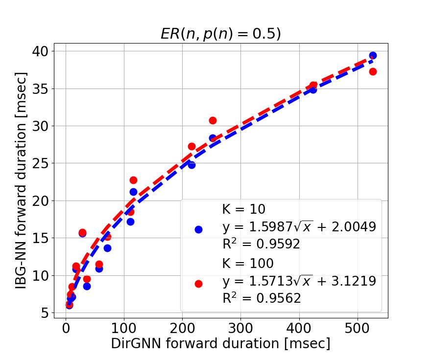
Figure 2: Runtime of K-IBG-NN (K=10, 100) vs. DirGNN forward pass duration on $\mathrm{ER}(n,p=0.5)$ graphs.

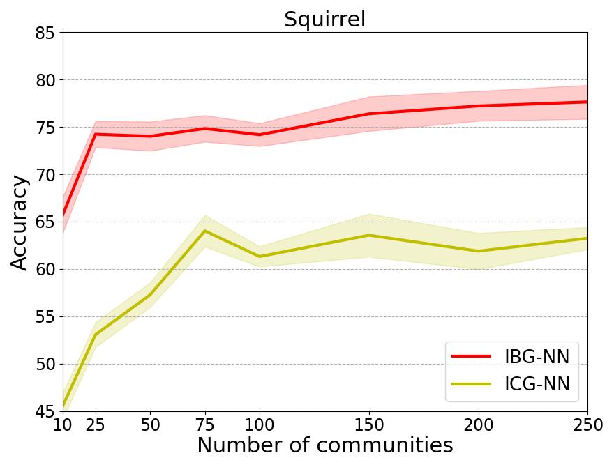
Figure 3: Accuracy of IBG-NN and ICG-NN on the Squirrel dataset as a function of the number of communities.

Setup.

We perform a comparison between IBG-NNs and ICG-NNs on the non-sparse Squirrel graph (Pei et al., 2020). We follow the 10 data splits of Pei et al. (2020); Li et al. (2022b) for Squirrel and report the accuracy and standard deviation.

Results.

In Figure˜3, IBG-NNs exhibit significantly improved performance compared to ICG-NNs. For a small number of communities (10), IBG-NNs achieve 66% accuracy, whereas ICG-NNs achieve only 45%, further demonstrating that IBG-NNs can reach competitive performance while being efficient. This performance gap persists as the number of communities increases.

7.3 Subgraph SGD for large graph

Setup. We evaluate IBG-NN and its predecessor ICG-NN on the large graphs Reddit Hamilton et al. (2017a) and Flickr Zeng et al. (2019) datasets, following the data split provided in Zheng et al. (2024). Accuracy and standard deviation are reported for experiments conducted with $5$ different seeds over varying condensation ratios $r=\frac{M}{N}$, where $N$ is the total number of nodes, and $M$ is the number of sampled nodes.

The graph coarsening baselines Coarsening Huang et al. (2021), Random Huang et al. (2021), Herding Welling (2009), K-Center Sener and Savarese (2017), One-Step Jin et al. (2022) and the graph condensation baselines DC-Graph Zhao et al. (2020), GCOND Jin et al. (2021), SFGC Zheng et al. (2024) and GC-SNTK Wang et al. (2024) are taken from Zheng et al. (2024); Wang et al. (2024). We use Adam optimizaer and report all hyperparameters in Appendix˜O.

Results. Table˜1 demonstrates that subgraph SGD IBG-NN achieves state-of-the-art performance across all sampling rates, surpassing all other coarsening and condensation methods that operate on the full graph in memory, while also improving upon the performance of its predecessor, ICG-NN. A comparison between graph coarsening methods and IBG-NNs can be found in Appendix˜A.

8 Conclusion

We proved a new semi-constructive variant of the weak regularity lemma, in which the required number of communities for a given approximation error is independent of any property of the graph, including the number of nodes and sparsity level, while in previous formulations of the lemma the number of communities increased as the graph became sparser. Our formulation is achieved by introducing the densifying cut similarity, which allows the approximating IBG to effectively densify the target graph. This enables fitting IBGs of very low rank ($K={\mathcal{O}}(1)$) to large sparse graphs, while previous works required the target graph to be both large and dense in order to obtain low rank approximations. We introduced IBG-NNs– a signal processing approach which operates on the IBG instead of the graph, and has ${\mathcal{O}}(N)$ time and memory complexity due to the number of communities being ${\mathcal{O}}(1)$. IBG-NNs demonstrate state-of-the-art performance in multiple domains: node classification on directed graphs, spatio-temporal graph analysis, and knowledge graph completion.

The main limitation of IBG-NNs is that they are not naturally transferrable between graphs: an IBG-NN learned on one graph cannot be applied to another graph, as there is no canonical way to match communities between different graphs. Future work will study strategies to transfer learned IBG-NNs between graphs.

Appendix A Related work

Intersecting Community Graphs (ICG). Our work continues the ICG setting of [Finkelshtein et al., 2024], which introduces a weak regularity lemmas for practical graph computations. The work of [Finkelshtein et al., 2024] presented a pipeline for operating on undirected, non-sparse graphs. Similarly to our work, [Finkelshtein et al., 2024] follow a two stage procedure. In the first stage, the graph is approximated by learning a factorization into undirected communities, forming what they call an Intersecting Community Graph (ICG). In the second stage, the ICG is used to enrich a neural network operating on the node features and community graph without using the original edge connectivity. This setup allows for more efficient computation, both in terms of runtime and memory, since the full edge structure of the graph, used in standard GNNs, can be replaced with a much smaller community-level graph—especially useful for graphs with a high average degree. The constructive weak regularity lemma presented in Finkelshtein et al. [2024] shows any graph can be approximated in cut-norm, regardless of its size, by minimizing the easy to compute Frobenius error.

More concretely, an ICG with $K$ communities is just like an IBG with only node features (no edge-features), but with the transmitting and receiving communities being equal $\mathbf{U}=\mathbf{V}$. Namely, an ICG can be represented by a triplet of community affiliation matrix ${\bm{Q}}\in{\mathbb{R}}^{N\times K}$, community magnitude vector ${\bm{r}}\in{\mathbb{R}}^{K}$, and community feature matrix $\mathbf{F}\in{\mathbb{R}}^{K\times D}$. An ICG $({\bm{C}},{\bm{P}})$ with adjacency matrix ${\bm{C}}$ and signal ${\bm{P}}$ is then given by

$${\bm{C}}={\bm{Q}}\operatorname{diag}({\bm{r}}){\bm{Q}}^{\top}\quad\text{and}\quad{\bm{P}}={\bm{Q}}{\bm{F}},$$

where $\operatorname{diag}({\bm{r}})$ is the diagonal matrix in ${\mathbb{R}}^{K\times K}$ with ${\bm{r}}$ as its diagonal elements. Here, $K$ is the number of communities, $N$ is the number of nodes, and $E$ is the number of edges.

When approximating a graph-signal $({\bm{A}},{\bm{S}})$, the measure of accuracy, or error, in Finkelshtein et al. [2024] is defined to be the standard (unweighted) cut metric $\left\|({\bm{A}},{\bm{S}})-({\bm{C}},{\bm{P}})\right\|_{\square}$. The semi-constructive regularity lemma of Finkelshtein et al. [2024] states that it is enough to minimize the standard Forbenius error $\left\|({\bm{A}},{\bm{S}})-({\bm{C}},{\bm{P}})\right\|_{\rm F}$ in order to guarantee

$$\left\|({\bm{A}},{\bm{S}})-({\bm{C}},{\bm{P}})\right\|_{\square}={\mathcal{O}}(N/\sqrt{KE}),$$ (10)

Looking at (10) it is clear that in order to guarantee a small approximation error in cut metric, the number of communities must increase as $N/\sqrt{E}$ becomes larger. Specifically, the number of communities $K$ is independent of the size of the graph only when $E=N^{2}$, i.e., the graph is dense. Hence, the ICG method falls short for sparse graphs

Our IBG method solves this shortcoming, and more. For exmaple, a main contribution of our method is a densification mechanism, supported by our novel densifying cut similarity measure and out densifying regularity lemma, which is a non-trivial continuation and extension of the semi-constructive weak regularity lemma of Finkelshtein et al. [2024]. Please see Appendix J for a detailed comparison of our ICB method to ICG.

Cluster Affiliation models (BigClam and PieClam). A similar work is PieClam [Zilberg and Levie, 2024], extending the well known BigClam model [Yang and Leskovec, 2013], which builds a probabilistic model of graphs as intersections of overlapping communities. While BigClam only allows communities with positive coefficients, which limits the ability to approximate many graphs, like bipartite graphs, PieClam formulates a graph probabilistic autoencoder that also includes negative communities. This allows approximately encoding any dense graph with a fixed budget of parameters per node. We note that as opposed to ICG and PieClam, which can only theoretically approximate dense graphs with ${\mathcal{O}}(1)$ communities, our IBG method can approximate both sparse and dense graph with ${\mathcal{O}}(1)$ communities via the densification mechanism (the densifying constructive regularity lemma with respect to the densifying cut similarity).

GNNs for directed graphs. The standard practice in GNN design is to assume that the graph is undirected [Kipf and Welling, 2017]. However, this assumption not only alters the input data by discarding valuable directional information, but also overlooks the empirical evidence demonstrating that leveraging edge directionality can significantly enhance performance Rossi et al. [2024]. For instance, DirGNN Rossi et al. [2024] extends message-passing neural networks (MPNNs) to directed graphs, while Geisler et al. [2023] adapts transformers for the same purpose. FaberNet Koke and Cremers [2024] generalizes spectral convolutions to directed graphs, all of which have led to improved performance. Furthermore, the proper handling of directed edges has enabled Maskey et al. [2024] to extend the concept of oversmoothing to directed graphs, providing deeper theoretical insights. IBG-NNs also capitalize on edge directionality, achieving notable performance improvements over their predecessor ICG-NNs [Finkelshtein et al., 2024], as demonstrated in Section˜L.4. When compared to existing GNNs designed for directed graphs, IBG-NNs offer a more efficient approach to signal processing. Specifically, for IBG-NNs to outperform message-passing-based GNNs in terms of efficiency, the condition $KN<E$ must hold, which is typically satisfied in practice for most graphs. This efficiency advantage allows IBG-NNs to make better use of the input edges while being more efficient than traditional GNNs for directed graphs.

Graph Pooling GNNs. Graph pooling GNNs generate a sequence of increasingly coarsened graphs by aggregating neighboring nodes into "super-nodes" Ying et al. [2018], Bianchi et al. [2020], where standard message-passing is applied on the intermediate coarsened graphs. Similarly, in IBG-NNs, the signal is projected, but onto overlapping blocks rather than disjoint clusters, with several additional key distinctions: (1) The blocks in IBG-NNs are overlapping and cover large regions of the graph, allowing the method to preserve fine-grained, high-frequency signal details during projection, unlike traditional graph pooling approaches. (2) Operations on community features in IBG-NNs possess a global receptive field, enabling the capture of broader structural patterns across the graph – an extremely difficult task for local graph pooling approach. (3) IBG-NNs diverge from the conventional message-passing framework: the flattened community feature vector, which lacks symmetry, is processed by a general multilayer perceptron (MLP), whereas message-passing neural networks (MPNNs) apply the same function uniformly to all edges. (4) IBG-NNs operate exclusively on an efficient data structure, offering both theoretical guarantees and empirical evidence of significantly improved computational efficiency compared to graph pooling methods.

Graph reduction methods. Graph reduction aims to reduce the size of the graph while preserving key information. It can be categorized into three main approaches: graph sparsification, graph coarsening and graph condensation. Graph sparsification methods Hamilton et al. [2017a], Zeng et al. [2019], Chen et al. [2018], Rong et al. [2020] approximate a graph by retaining only a subset of its edges and nodes, often employing random sampling techniques. Graph coarsening Fey et al. [2020], Huang et al. [2021] clusters sets of nodes into super-nodes while aggregating inter-group edges into super-edges, aiming to preserve structural properties such as the degree distribution Zhou et al. [2023]. Graph condensation Jin et al. [2021] generates a smaller graph with newly created nodes and edges, designed to maintain the performance of GNNs on downstream tasks.

While subgraph SGD in IBG-NNs also involves subsampling, it differs fundamentally by providing a provable approximation of the original graph. This contrasts with graph sparsification for example – where some, hopefully good heuristic-based sampling is often employed. More importantly, subgraph IBG-NNs offer a subgraph sampling approach for cases where the original graph is too large to fit in memory. This contrasts with the aforementioned coarsening and condensation methods, which lack a strategy for managing smaller data structures during the computation of the compressed graph.

Graph reduction methods generally rely on locality, applying message-passing on the reduced graph. In particular, condensation techniques require ${\mathcal{O}}(EM)$ operations to construct a smaller graph Jin et al. [2021], Zheng et al. [2024], Wang et al. [2024], where $E$ is the number of edges in the original graph and $M$ is the number of nodes in the condensed graph. In contrast, IBG-NNs estimate the IBG with only ${\mathcal{O}}(E)$ operations.

Furthermore, while conventional reduction methods process representations on either an iteratively coarsened graph or mappings between the full and reduced graphs, IBG-NNs incorporate fine-grained node information at every layer, leading to richer representations.

Cut metric in graph machine learning. The cut metric is a useful similarity measure, which can separate any non-isomorphic graphons Lovász [2012]. This makes the cut metric particularity useful in deriving new theoretical insights for graph machine learning. For instance, [Levie, 2023] demonstrated that GNNs with normalized sum aggregation cannot separate graph-signals that are close to each other in cut metric. Using the cut distance as a theoretical tool, [Maskey et al., 2023] proves that spectral GNNs with continuous filters are transferable between graphs in sequences of that converge in homomorphism density. Finkelshtein et al. [2024] introduced a semi constructive weak regularity lemma and used it to build new algorithms on large undirected non-sparse graphs. In this work we introduce a new graph similarity measure – the densifying cut similarity, which gives higher importance to edges than non-edges in a graph. This allows us to approximate any graph using a set of overlapping bipartite components, where the size of the set only depends on the error tolerance. Similarly to Finkelshtein et al. [2024], we present a semi constructive weak regularity lemma. As oppose to Finkelshtein et al. [2024], using our novel similarity measure, our regularity lemma can be used to build new algorithms on large directed graphs which are sparse.

Appendix B The weak regularity lemma

Consider a graph $G$ with a node set $\mathcal{V}=[N]=\{1,\dots,N\}$ and an edge set ${\mathcal{E}}\subseteq\mathcal{V}\times\mathcal{V}$. We define an equipartition $\mathcal{P}=\{{\mathcal{V}}_{1},\ldots{\mathcal{V}}_{k}\}$ as a partition of ${\mathcal{V}}$ into $k$ sets where $\left|\left|{\mathcal{V}}_{i}\right|-\left|{\mathcal{V}}_{j}\right|\right|\leq 1$ for every $1\leq i,j\leq k$. For any pair of subsets $\mathcal{U},\mathcal{S}\subset{\mathcal{V}}$ denote by $e_{G}(\mathcal{U},\mathcal{S})$ the number of edges between $\mathcal{U}$ and $\mathcal{S}$. Now, consider two node subsets $\mathcal{U},\mathcal{S}\subset{\mathcal{V}}$. If the edges between ${\mathcal{V}}_{i}$ and ${\mathcal{V}}_{j}$ were to be uniformly and independently distributed, then the expected number of edges between $\mathcal{U}$ and $\mathcal{S}$ would be

$$e_{\mathcal{P}(\mathcal{U},\mathcal{S})}:=\sum_{i=1}^{k}\sum_{j=1}^{k}\frac{e_{G}({\mathcal{V}}_{i},{\mathcal{V}}_{j})}{\left|{\mathcal{V}}_{i}\right|\left|{\mathcal{V}}_{j}\right|}\left|{\mathcal{V}}_{i}\cap\mathcal{U}\right|\left|{\mathcal{V}}_{j}\cap\mathcal{S}\right|.$$

Using the above, we define the irregularity:

$$\mathrm{irreg}_{G}(\mathcal{P})=\max_{\mathcal{U},\mathcal{S}\subset{\mathcal{V}}}\left|e_{G}(\mathcal{U},\mathcal{S})-e_{\mathcal{P}}(\mathcal{U},\mathcal{S})\right|/\left|{\mathcal{V}}\right|^{2}.$$ (11)

The irregularity measures how non-random like the edges between $\{{\mathcal{V}}_{j}\}$ behave.

We now present the weak regularity lemma.

Theorem B.1 (Weak Regularity Lemma Frieze and Kannan [1999]).

For every $\epsilon>0$ and every graph $G=({\mathcal{V}},\mathcal{E})$, there is an equipartition $\mathcal{P}=\{{\mathcal{V}}_{1},\ldots,{\mathcal{V}}_{k}\}$ of ${\mathcal{V}}$ into $k\leq 2^{c/\epsilon^{2}}$ classes such that $\mathrm{irreg}_{G}(\mathcal{P})\leq\epsilon$. Here, $c$ is a universal constant that does not depend on $G$ and $\epsilon$.

The weak regularity lemma states that any large graph $G$ can be approximated by a weighted graph $G^{\epsilon}$ with node set ${\mathcal{V}}^{\epsilon}=\{{\mathcal{V}}_{1},\ldots,{\mathcal{V}}_{k}\}$. The nodes of $G^{\epsilon}$ represent clusters of nodes from $G$, and the edge weight between two clusters ${\mathcal{V}}_{i}$ and ${\mathcal{V}}_{j}$ is given by $\frac{e_{G}({\mathcal{V}}_{i},{\mathcal{V}}_{j})}{|{\mathcal{V}}_{i}||{\mathcal{V}}_{j}|}$. In this context, an important property of the irregularity $\mathrm{irreg}_{G}(\mathcal{P})$ is that it can be seen as the cut metric between the $G$ and a SBM based on $G^{\epsilon}$. For each node $i$ denote by ${\mathcal{V}}_{q_{i}}\in\mathcal{P}$ the partition set that contains the node. Given $G^{\epsilon}$, construct a new graph $G^{\mathcal{P}}$ with $N$ nodes, whose adjacency matrix ${\bm{A}}^{\mathcal{P}}=(a^{\mathcal{P}}_{i,j})_{i,j=1}^{|{\mathcal{V}}|}$ is defined by

$$a^{\mathcal{P}}_{i,j}=\frac{e_{G}({\mathcal{V}}_{q_{i}},{\mathcal{V}}_{q_{j}})}{|{\mathcal{V}}_{q_{i}}||{\mathcal{V}}_{q_{j}}|},$$

. Let ${\bm{A}}$ be the adjacency matrix of $G$. It can be shown that

$$\left\|{\bm{A}}-{\bm{A}}^{\mathcal{P}}\right\|_{\square}=\mathrm{irreg}_{G}(\mathcal{P}),$$

which shows that the weak regularity lemma can be expressed in terms of cut norm rather than irregularity.

Appendix C Graphons and norms

Kernel.

A kernel $Y$ is a measurable function $Y:[0,1]^{2}\rightarrow[-1,1]$.

Graphon.

A graphon [Borgs et al., 2008, Lovász, 2012] is a measurable function $W:[0,1]^{2}\rightarrow[0,1]$. A graphon can be seen as a weighted graph, where the node set is the interval $[0,1]$, and for any pair of nodes $x,y\in[0,1]$, the weight of the edge between $x$ and $y$ is $W(x,y)$, which can also be seen as the probability of having an edge between $x$ and $y$. We note that in the standard definition a graphon is defined to be symmetric, but we remove this restriction in our construction.

Kernel-signal and Graphon-signal.

A kernel-signal is a pair $(Y,y)$ where $Y$ is a kernel and $y:[0,1]\rightarrow\mathbb{R}^{D}$ is a measurable function. A graphon-signal is defined similarly with a graphon in place of a kernel.

Induced graphon-signal.

Consider an interval equipartition $\mathcal{I}_{m}=\{I_{1},\ldots,I_{m}\}$, a partition of $[0,1]$ into disjoint intervals of equal length. Given a graph $G$ with an adjacency matrix ${\bm{A}}$, the induces graphon $W_{\bm{A}}$ is the graphon defined by $W_{\bm{A}}(x,y)={\bm{A}}_{\lceil xm\rceil\lceil ym\rceil}$, where we use the convention that $\lceil 0\rceil=1$. Notice that $W_{\bm{A}}$ is a piecewise constant function on the equipartition $\mathcal{I}_{m}$. As such, a graph of $m$ nodes can be identified by its induced graphon that is piecewise constant on $\mathcal{I}_{m}$.

C.1 Weighted Frobenius and cut norm

Weighted Frobenius norm.

Let $q:[0,1]^{2}\rightarrow\left.\left[c,\infty\right.\right)$ be a measurable function in $\mathcal{L}^{\infty}([0,1]^{2})$, where $c>0$. We call such a $q$ a weight function. Consider the real weighted Lebesgue space $\mathcal{L}^{2}([0,1]^{2};q)$ defined with the inner product

$$\left\langle Y,Y^{\prime}\right\rangle_{q}:=\frac{1}{\left\|1\right\|_{1;q}}\iint_{[0,1]^{2}}Y(x,y)Y^{\prime}(x,y)q(x,y)dxdy,$$

where $1$ is the constant function $[0,1]^{2}\ni(x,y)\mapsto 1$ and $\left\|1\right\|_{1;q}=\iint q$. When $q=1$, we denote $\left\langle X,Z\right\rangle:=\left\langle X,Z\right\rangle_{1}$. Let $\alpha,\beta>0$. Consider the real Hilbert space $L^{2}([0,1]^{2};q)\times(L^{2}[0,1])^{D}$ defined with the weighted inner product

$$\left\langle(Y,y),(Y^{\prime},y^{\prime})\right\rangle_{q}=\left\langle(Y,y),(Y^{\prime},y^{\prime})\right\rangle_{q,\alpha,\beta}=\alpha\frac{1}{\left\|1\right\|_{1;q}}\iint_{[0,1]^{2}}Y(x,y)Y^{\prime}(x,y)q(x,y)dxdy+\frac{\beta}{D}\sum_{j=1}^{D}\int_{[0,1]}y_{j}(x)y_{j}^{\prime}(x)dx.$$

We call the corresponding weighted norm the weighted Frobenius norm, denoted by

$$\left\|(Y,y)\right\|_{{\rm F};q}=\left\|(Y,y)\right\|_{{\rm F};q,\alpha,\beta}=\sqrt{\alpha\left\|Y\right\|^{2}_{{\rm F};q}+\frac{\beta}{D}\sum_{j=1}^{D}\left\|y_{j}\right\|^{2}_{\mathrm{F}}},$$

where $\left\|Y\right\|^{2}_{{\rm F};q}=\left\langle Y,Y\right\rangle_{q}$ and $\left\|y_{j}\right\|^{2}_{\mathrm{F}}=\left\langle y_{j},y_{j}\right\rangle_{1}$.

Similarly, for a matrix-signal, we consider a weight matrix ${\bm{Q}}\in\left.\left[c,\infty\right.\right)^{N\times N}$, where $c>0$. For ${\bm{D}},{\bm{D}}^{\prime}\in{\mathbb{R}}^{N\times N}$, define the weighted inner product by

$$\left\langle{\bm{D}},{\bm{D}}^{\prime}\right\rangle_{{\bm{Q}}}:=\frac{1}{\left\|\mathbf{1}\right\|_{1;{\bm{Q}}}}\sum_{i,j\in[N]^{2}}d_{i,j}d^{\prime}_{i,j}q_{i,j},$$

where $\mathbf{1}\in\mathbb{R}^{N\times N}$ is the matrix with all entries equal to $1$, and $\left\|\mathbf{1}\right\|_{1;{\bm{Q}}}=\sum_{i,j\in[N]^{2}}q_{i,j}$. Define the weighted matrix-signal Frobenius norm by

$$\left\|({\bm{D}},{\bm{Z}})\right\|_{{\rm F};{\bm{Q}}}=\left\|({\bm{D}},{\bm{Z}})\right\|_{{\rm F};{\bm{Q}},\alpha,\beta}=\sqrt{\alpha\left\|{\bm{D}}\right\|^{2}_{{\rm F};{\bm{Q}}}+\frac{\beta}{D}\sum_{j=1}^{D}\left\|{\bm{z}}_{j}\right\|^{2}_{\mathrm{F}}},$$

where $\left\|{\bm{D}}\right\|^{2}_{{\rm F};{\bm{Q}}}=\left\langle{\bm{D}},{\bm{D}}\right\rangle_{{\bm{Q}}}$ and $\left\|{\bm{z}}_{j}\right\|^{2}_{\mathrm{F}}=\left\langle{\bm{z}}_{j},{\bm{z}}_{j}\right\rangle_{1}$.

Graphon weighted cut norm and cut metric.

A kernel-signal $(Y,y)$ is a pair where $Y:[0,1]^{2}\rightarrow[-1,1]$ and $y:[0,1]\rightarrow\mathbb{R}^{D}$ are measurable. Define for a kernel-signal $(Y,y)$ the weighted cut norm

$$\left\|(Y,y)\right\|_{\square;q,\alpha,\beta}=\left\|(Y,y)\right\|_{\square;q}=\frac{\alpha}{\left\|1\right\|_{1;q}}\sup_{\mathcal{U},\mathcal{V}}\left|\int_{\mathcal{U}}\int_{\mathcal{V}}Y(x,y)q(x,y)dxdy\right|+\beta\frac{1}{D}\sum_{j=1}^{D}\sup_{\mathcal{U}}\left|\int_{\mathcal{U}}y_{j}(x)dx\right|,$$

where the supremum is over the set of measurable subsets $\mathcal{U},\mathcal{V}\subset[0,1]$.

The weighted cut metric between two graphon-signals $(W,f)$ and $(W^{\prime},f^{\prime})$ is defined to be $\left\|(W,f)-(W^{\prime},f^{\prime})\right\|_{\square;q}$.

Graph-signal weighted cut norm and cut metric.

Define for a matrix-signal $({\bm{D}},{\bm{Z}})$, where ${\bm{D}}\in[-1,1]^{N\times N}$ and ${\bm{Z}}\in\mathbb{R}^{N\times D}$, the weighted cut norm

$$\left\|({\bm{D}},{\bm{Z}})\right\|_{\square;{\bm{Q}},\alpha,\beta}=\left\|({\bm{D}},{\bm{Z}})\right\|_{\square;{\bm{Q}}}=\alpha\left\|{\bm{D}}\right\|_{\square;{\bm{Q}}}+\beta\left\|{\bm{Z}}\right\|_{\square}$$

$$=\frac{\alpha}{\left\|\mathbf{1}\right\|_{1;{\bm{Q}}}}\max_{\mathcal{U},\mathcal{V}\subset[N]}\left|\sum_{i\in\mathcal{U}}\sum_{j\in\mathcal{V}}d_{i,j}q_{i,j}\right|+\frac{\beta}{DN}\sum_{j=1}^{D}\max_{\mathcal{U}\subset[N]}\left|\sum_{i\in\mathcal{U}}z_{i,j}\right|.$$

The weighted cut metric between two graph-signals $({\bm{A}},{\bm{s}})$ and $({\bm{A}}^{\prime},{\bm{s}}^{\prime})$ is defined to be $\left\|({\bm{A}},{\bm{s}})-({\bm{A}}^{\prime},{\bm{s}}^{\prime})\right\|_{\square;{\bm{Q}}}$. We note that this metric gives a meaningful notion of graph-signal similarity for graphs as long as their number of edges satisfy $\left\|\mathbf{1}\right\|_{1;{\bm{Q}}}=\Theta(E)$. All graphs with $E\ll\left\|\mathbf{1}\right\|_{1;{\bm{Q}}}$ have distance close to zero from each other, so the cut metric does not have a meaningful or useful separation power for such graphs.

Densifying cut similarity.

In this paper, we will focus on a special construction of a weighted cut norm, which we construct and motivate next.

In graph completion tasks, such as link prediction or knowledge graph reasoning, the objective is to complete a partially observed adjacency matrix. Namely, there is a set of known dyads $\mathcal{M}\subset[N]^{2}$, and the given data is the restriction of ${\bm{A}}$ to the known dyads

$${\bm{A}}|_{\mathcal{M}}:\mathcal{M}\rightarrow\{0,1\}.$$

The goal is then to find an adjacency matrix ${\bm{B}}$ that fits ${\bm{A}}$ on the known dyads, namely, ${\bm{B}}|_{\mathcal{M}}\approx{\bm{A}}|_{\mathcal{M}}$, with the hope that ${\bm{B}}$ also approximates ${\bm{A}}$ on the unknown dyads due to some inductive bias.

Recall that $\mathcal{E}$ denotes the set of edges of ${\bm{A}}$. We call $\mathcal{E}^{\rm c}=[N]^{2}\setminus\mathcal{E}$ the set of non-edges. The training set in graph completion consists of the edges $\mathcal{E}\cap\mathcal{M}$ and the non-edges $\mathcal{E}^{\rm c}\cap\mathcal{M}$. Typical methods, such as VGAE [Kipf and Welling, 2016] and TLC-GNN [Yan et al., 2021], define a loss of the form

$$l({\bm{B}})=\sum_{(n,m)\in\mathcal{M}\cap\mathcal{E}}c_{n,m}\psi_{1}(b_{n,m},a_{n,m})+\sum_{(n,m)\in\mathcal{M}\cap\mathcal{E}^{\rm c}}c_{n,m}\psi_{2}(b_{n,m},a_{n,m}),$$

where $\psi_{1},\psi_{2}:\mathbb{R}^{2}\rightarrow\mathbb{R}_{+}$ are dyad-wise loss functions and $c_{n,m}\in\mathbb{R}_{+}$ are weights. Many methods, like RotateE [Sun et al., 2019], HousE [Li et al., 2022a] and NBFNet [Zhu et al., 2021], give one weight $c_{n,m}=C$ for edges $(n,m)\in\mathcal{E}\cap\mathcal{M}$ and a smaller weight $c_{n,m}=c\ll C$ for non-edges $(n,m)\in\mathcal{E}^{\rm c}\cap\mathcal{M}$. The motivation is that for sparse graphs there are many more non-edges than edges, and giving the edges and non-edges the same weight would tend to produce learned ${\bm{B}}$ that does not put enough emphasis on the connectivity structure of ${\bm{A}}$. In practice, the smaller weight for non-edges is implemented implicitly by taking random samples from $\mathcal{M}$ during training, balancing the number of samples from $\mathcal{E}\cap\mathcal{M}$ and from $\mathcal{E}^{\rm c}\cap\mathcal{M}$. The samples from $\mathcal{E}^{\rm c}\cap\mathcal{M}$ are called negative samples.

Remark C.1.

In this paper we interpret such an approach as learning a densified version of ${\bm{A}}$. Namely, by putting less emphasis on non-edges, the matrix ${\bm{B}}$ roughly fits the structure of ${\bm{A}}$, but with a higher average degree.

Motivated by the above discussion, we also define a densifying version of cut distance. Given a target unweighted adjacency matrix ${\bm{A}}=(a_{i,j})_{i,j=1}^{N}$ to be approximated, we consider the weight matrix ${\bm{Q}}=e\mathbf{1}+(1-e){\bm{A}}$ for some small $e$ and $\mathbf{1}$ being the all 1 matrix. Denote the number of edges by $E=\left|\mathcal{E}\right|$. Next, we would like to choose $e$ to reflect some desired balance between edges and non-edges. Since the number of non-edges is $N^{2}-E$ and the number of edges is $E$, we choose $e$ in such a way that $e-(E/N^{2})e=\Gamma E/N^{2}$ for some $\Gamma>0$, namely,

$$e=e_{E,\Gamma}=\frac{\Gamma E/N^{2}}{1-(E/N^{2})}.$$ (12)

The interpretation of $\Gamma$ is the proposition of sampled non-edges when compared with the edges. Namely, the weight matrix ${\bm{Q}}=e+(1-e){\bm{A}}$ effectively simulates taking $\Gamma E$ negative samples and $E$ samples. Observe that

$$\left\|{\bm{A}}\right\|_{{\mathrm{F}};e\mathbf{1}+(1-e){\bm{A}}}^{2}=\frac{1}{\sum_{i,j\in[N]^{2}}q_{i,j}}\sum_{i,j\in[N]^{2}}a_{i,j}q_{i,j}=\frac{E/N^{2}}{e+(1-e)E/N^{2}}=1/(\Gamma+1).$$

To standardize the above similarity measure, we normalize it and define the weighted Frobenius norm $(1+\Gamma)\left\|{\bm{B}}\right\|_{{\mathrm{F}};{\bm{Q}}_{{\bm{A}}}}$ and weighted cut norm $(1+\Gamma)\left\|{\bm{B}}\right\|_{\square;{\bm{Q}}_{{\bm{A}}}}$, where

$${\bm{Q}}_{{\bm{A}}}={\bm{Q}}_{{\bm{A}},\Gamma}:=e_{E,\Gamma}\mathbf{1}+(1-e_{E,\Gamma}){\bm{A}},$$ (13)

and where $e_{E,\Gamma}$ is defined in (12). We now have

$$(1+\Gamma)\left\|{\bm{A}}\right\|_{{\mathrm{F}};{\bm{Q}}_{{\bm{A}}}}=1.$$ (14)

This standardization assures that merely increasing $\Gamma$ in the definition of the cut metric $(1+\Gamma)\left\|{\bm{A}}-{\bm{B}}\right\|_{{\mathrm{F}};{\bm{Q}}_{{\bm{A}}}}$ would not lead to a seemingly better approximation. The above discussion leads to the following definition.

Definition C.1.

Let ${\bm{A}}\in\{0,1\}^{N\times N}$ be an unweighted adjacency matrix, and $\Gamma>0$. The densifying cut similarity between the target ${\bm{A}}$ and any adjacency matrix ${\bm{B}}\in\mathbb{R}^{N\times N}$ is defined to be

$$\sigma_{\square}({\bm{A}}||{\bm{B}})=\sigma_{\square;\Gamma}({\bm{A}}||{\bm{B}}):=(1+\Gamma)\left\|{\bm{A}}-{\bm{B}}\right\|_{\square;{\bm{Q}}_{{\bm{A}}}},$$

where ${\bm{Q}}_{{\bm{A}}}$ is defined in (13). Given $\alpha,\beta>0$ such that $\alpha+\beta=1$, the densifying cut similarity between the target graph-signal $({\bm{A}},{\bm{X}})$ and the graph-signal $({\bm{A}}^{\prime},{\bm{X}}^{\prime})$ is defined to be

$$\sigma_{\square}\big{(}({\bm{A}},{\bm{X}})||({\bm{A}}^{\prime},{\bm{X}}^{\prime})\big{)}=\sigma_{\square;\alpha,\beta,\Gamma}\big{(}({\bm{A}},{\bm{X}})||({\bm{A}}^{\prime},{\bm{X}}^{\prime})\big{)}:=\alpha\sigma_{\square;\Gamma}({\bm{A}}||{\bm{B}})+\beta\left\|{\bm{X}}-{\bm{X}}^{\prime}\right\|_{\square}.$$

We moreover note that the similarity measure $\sigma_{\square}({\bm{A}}||{\bm{B}})$ is not symmetric, and hence not a metric. The first entry ${\bm{A}}$ in $\sigma_{\square}({\bm{A}}||{\bm{B}})$ is interpreted as the thing to be approximated, and the second entry ${\bm{B}}$ as the approximant. Here, when fitting an IBG to a graph, ${\bm{A}}$ is a constant, and ${\bm{B}}$ is the variable.

Appendix D Proof of the semi-constructive densifying directional soft weak regularity lemma

In this section we prove a version of the constructive weak regularity lemma for asymmetric graphon signals. Prior information regarding cut-distance, the original formulation of the weak regularity lemma and it’s constructive version for symmetric graphon-signals can be found in (Finkelshtein et al., 2024, Appendix A, B).

D.1 Intersecting block graphons

Below, we extend the definition of IBGs for graphons. The construction is similar to the one in Appendix B.3 of [Finkelshtein et al., 2024], where ICGs are extended to graphons. Denote by $\chi$ the set of all indicator functions of measurable subset of $[0,1]$

$$\chi=\{\mathbbm{1}_{u}\ |\ u\subset[0,1]\text{ measurable}\}.$$

Definition D.1.

A set ${\mathcal{Q}}$ of bounded measurable functions $q:[0,1]\rightarrow{\mathbb{R}}$ that contains $\chi$ is called a soft affiliation model.

For the case of node level graphon-signals, we use the following definition:

Definition D.2.

Let $D\in{\mathbb{N}}$. Given a soft affiliation model ${\mathcal{Q}}$, the subset $[{\mathcal{Q}}]$ of $L^{2}[0,1]^{2}\times(L^{2}[0,1])^{D}$ of all elements of the form $(au(x)v(y),bu(z)+cv(z))$, with $u,v\in{\mathcal{Q}}$, $a\in{\mathbb{R}}$ and $b,c\in{\mathbb{R}}^{D}$, is called the soft rank-1 intersecting block graphon (IBG) model corresponding to ${\mathcal{Q}}$. Given $K\in{\mathbb{N}}$, the subset $[{\mathcal{Q}}]_{K}$ of $L^{2}[0,1]^{2}\times(L^{2}[0,1])^{D}$ of all linear combinations of $K$ elements of $[{\mathcal{Q}}]$ is called the soft rank-$K$ IBG model corresponding to ${\mathcal{Q}}$. Namely, $(C,p)\in[{\mathcal{Q}}]_{K}$ if and only if it has the form

$$C(x,y)=\sum_{k=1}^{K}a_{k}u_{k}(x)v_{k}(y)\quad\text{and}\quad p(z)=\sum_{k=1}^{K}b_{k}u_{k}(z)+c_{k}v_{k}(z)$$

where $(u_{k})_{k=1}^{K}\in{\mathcal{Q}}^{K}$ are called the target community affiliation functions, $(v_{k})_{k=1}^{K}\in{\mathcal{Q}}^{K}$ are called the source community affiliation functions, $(a_{k})_{k=1}^{K}\in{\mathbb{R}}^{K}$ are called the community affiliation magnitudes, $(b_{k})_{k=1}^{K}\in{\mathbb{R}}^{K\times D}$ are called the target community features, and $(c_{k})_{k=1}^{K}\in{\mathbb{R}}^{K\times D}$ the source community features. Any element of $[\mathcal{Q}]_{K}$ is called an intersecting block graphon-signal (IBG).

D.2 The semi-constructive weak regularity lemma in Hilbert space

In the following subsection we prove our version of the constructive weak graphon-signal regularity lemma.

László Miklós Lovász [2007] extended the weak regularity lemma to graphons. They showed that the lemma follows from a more general result about approximation in Hilbert spaces – the weak regularity lemma in Hilbert spaces [László Miklós Lovász, 2007, Lemma 4]. We extend this result to have a constructive form, which we later use to prove Theorem˜4.1. For completeness, we begin by stating the original weak regularity lemma in Hilbert spaces from [László Miklós Lovász, 2007].

Lemma D.1 ([László Miklós Lovász, 2007]).

Let ${\mathcal{K}}_{1},{\mathcal{K}}_{2},\ldots$ be arbitrary nonempty subsets (not necessarily subspaces) of a real Hilbert space ${\mathcal{H}}$. Then, for every $\epsilon>0$ and $g\in{\mathcal{H}}$ there is $m\leq\lceil 1/\epsilon^{2}\rceil$ and $(f_{i}\in{\mathcal{K}}_{i})_{i=1}^{m}$ and $(\gamma_{i}\in{\mathbb{R}})_{i=1}^{m}$, such that for every $w\in{\mathcal{K}}_{m+1}$

$$\bigg{|}\left\langle w,g-(\sum_{i=1}^{m}\gamma_{i}f_{i})\right\rangle\bigg{|}\leq\epsilon\ \left\|w\right\|\left\|g\right\|.$$

Finkelshtein et al. [2024] introduced a version of Lemma D.1 (Lemma B.3 therein) with a ”more constructive flavor.” They provide a result in which the approximating vector $\sum_{i=1}^{m}\gamma_{i}f_{i}$ is given as the solution to a "manageable" optimization problem, whereas the original lemma in [László Miklós Lovász, 2007] only proves the existence the approximating vector. Below, we give a similar result to[Finkelshtein et al., 2024, Lemma B.3.], where the constructive aspect is further improved. While [Finkelshtein et al., 2024] showed that the optimization problems leads to an approximate minimizer in high probability, they did not provide a way to evaluate if indeed this “good” event of high probability occurred. In contrast, we formulate this lemma in such a way that leads to a deterministic approach for checking if the good event happened. In the discussion after Lemma˜D.2, we explain this in detail.

Lemma D.2.

Let $\{{\mathcal{K}}_{j}\}_{j\in\mathbb{N}}$ be a sequence of nonemply subsets of a real Hilbert space ${\mathcal{H}}$. Let $K\in\mathbb{N}$, $\delta\geq 0$, let $R\geq 1$ such that $K/R\in\mathbb{N}$, let $\delta>0$, and let $g\in{\mathcal{H}}$. For every $k\in\mathbb{N}$, let

$$\eta_{k}=(1+\delta)\inf_{\bm{\kappa},\mathbf{h}}\|g-\sum_{i=1}^{k}\kappa_{i}h_{i}\|^{2}$$

where the infimum is over $\bm{\kappa}=\{\kappa_{1},\ldots,\kappa_{k}\}\in{\mathbb{R}}^{k}$ and $\mathbf{h}=\{h_{1},\ldots,h_{k}\}\in\mathcal{K}_{1}\times\ldots\times\mathcal{K}_{k}$. Then,

1. For every $m\in\mathbb{N}$, any vector of the form

   $$g^{*}=\sum_{j=1}^{m}\gamma_{j}f_{j}\quad\text{\ \ such that\ \ }\quad\bm{\gamma}=(\gamma_{j})_{j=1}^{m}\in\mathbb{R}^{m}\quad\text{and}\quad\mathbf{f}=(f_{j})_{j=1}^{m}\in\mathcal{K}_{1}\times\ldots\times\mathcal{K}_{m}$$ (15)

   that gives a close-to-best Hilbert space approximation of $g$ in the sense that

   $$\|g-g^{*}\|\leq\eta_{m},$$ (16)

   also satisfies

   $$\forall w\in{\mathcal{K}}_{m+1},\quad\left|\left\langle w,g-g^{*}\right\rangle\right|\leq\left\|w\right\|\sqrt{\eta_{m}-\frac{\eta_{m+1}}{1+\delta}}.$$ (17)

2. If $m$ is uniformly randomly sampled from $[K]$, then in probability $1-\frac{1}{R}$ (with respect to the choice of $m$),

   $$\left\|w\right\|\sqrt{\eta_{m}-\frac{\eta_{m+1}}{1+\delta}}\leq\left\|w\right\|\left\|g\right\|\sqrt{\frac{\delta}{1+\delta}+\frac{R(1+\delta)}{K}}.$$ (18)

   Specifically, in probability $1-\frac{1}{R}$, any vector of the form (15) which satisfy (16), also satisfies

   $$\forall w\in{\mathcal{K}}_{m+1},\quad\left|\left\langle w,g-g^{*}\right\rangle\right|\leq\left\|w\right\|\left\|g\right\|\sqrt{\frac{\delta}{1+\delta}+\frac{R(1+\delta)}{K}}.$$ (19)

The lemma is used as follows. We choose $m$ at random. We know by Item˜2 that in high probability the approximation is good (i.e. (19) is satisfied), but we are not certain. For certainty, we use the deterministic bound (17), which gives a certificate for a specific $m$. Namely, given a realization of $m$, we can estimate the right-hand-side of (17), which is also the left-hand-side of the probabilistic bound (18). For that, we find the $(m+1)$’th error $\eta_{m+1}$, solving another optimization problem, and verify that (18) is satisfied for $m$. If it is not, we resample $m$ and repeat. The expected number of times we need to repeat this until we get a small error is $R/(R-1)$.

Hence, under an assumption that the we can find a close to optimum $\left\|g-g^{*}\right\|$ for a given $m$ in $T_{K}$ operations, we can find in probability 1 a vector $g^{*}$ in the span of $\mathcal{K}_{1},\ldots,\mathcal{K}_{K}$ that solves (19) with expected number of operations $T_{K}R/(R-1)$.

Proof of Lemma D.2.

Let $K>0$. Let $R\geq 1$ such that $K/R\in\mathbb{N}$. For every $k$, let

$$\eta_{k}=(1+\delta)\inf_{\bm{\kappa},\mathbf{h}}\|g-\sum_{i=1}^{k}\kappa_{i}h_{i}\|^{2}$$

where the infimum is over $\bm{\kappa}=\{\kappa_{1},\ldots,\kappa_{k}\}\in{\mathbb{R}}^{k}$ and $\mathbf{h}=\{h_{1},\ldots,h_{k}\}\in\mathcal{K}_{1}\times\ldots\times\mathcal{K}_{k}$.

Note that every

$$g^{*}=\sum_{j=1}^{m}\gamma_{j}f_{j}$$ (20)

that satisfies

$$\left\|g-g^{*}\right\|^{2}\leq\eta_{m}$$

also satisfies: for any $w\in\mathcal{K}_{m+1}$ and every $t\in{\mathbb{R}}$,

$$\left\|g-(g^{*}+tw)\right\|^{2}\geq\frac{\eta_{m+1}}{1+\delta}=\frac{\eta_{m}+\eta_{m+1}-\eta_{m}}{1+\delta}\geq\frac{\left\|g-g^{*}\right\|^{2}}{1+\delta}-\frac{\eta_{m}-\eta_{m+1}}{1+\delta}.$$

This can be written as

$$\forall t\in\mathbb{R},\quad\left\|w\right\|^{2}t^{2}+2\left\langle w,g-g^{*}\right\rangle t+\frac{\eta_{m}-\eta_{m+1}}{1+\delta}+(1-\frac{1}{1+\delta})\left\|g-g^{*}\right\|^{2}\geq 0.$$ (21)

The discriminant of this quadratic polynomial is

$$4\left\langle w,g-g^{*}\right\rangle^{2}-4\left\|w\right\|^{2}\Big{(}\frac{\eta_{m}-\eta_{m+1}}{1+\delta}+(1-\frac{1}{1+\delta})\left\|g-g^{*}\right\|^{2}\Big{)}$$

and it must be non-positive to satisfy the inequality (21), namely

$$4\left\langle w,g-g^{*}\right\rangle^{2}\leq 4\left\|w\right\|^{2}\Big{(}\frac{\eta_{m}-\eta_{m+1}}{1+\delta}+(1-\frac{1}{1+\delta})\left\|g-g^{*}\right\|^{2}\Big{)}\leq 4\left\|w\right\|^{2}\Big{(}\frac{\eta_{m}-\eta_{m+1}}{1+\delta}+(1-\frac{1}{1+\delta})\eta_{m}\Big{)}$$

$$\leq 4\left\|w\right\|^{2}\Big{(}\eta_{m}-\frac{\eta_{m+1}}{1+\delta}\Big{)},$$

which proves

$$\left|\left\langle w,g-g^{*}\right\rangle\right|\leq\left\|w\right\|\sqrt{\eta_{m}-\frac{\eta_{m+1}}{1+\delta}},$$

which proves Item˜1.

For Item˜2, note that $\left\|g\right\|^{2}\geq\frac{\eta_{1}}{1+\delta}\geq\frac{\eta_{2}}{1+\delta}\geq\ldots\geq 0$. Therefore, there is a subset of at least $(1-\frac{1}{R})K+1$ indices $m$ in $[K]$ such that $\eta_{m}\leq\eta_{m+1}+\frac{R(1+\delta)}{K}\left\|g\right\|^{2}$. Otherwise, there are $\frac{K}{R}$ indices $m$ in $[K]$ such that $\eta_{m+1}<\eta_{m}-\frac{R(1+\delta)}{K}\left\|g\right\|^{2}$, which means that

$$\eta_{K}<\eta_{1}-\frac{K}{R}\frac{R(1+\delta)}{K}\left\|g\right\|^{2}\leq(1+\delta)\left\|g\right\|^{2}-(1+\delta)\left\|g\right\|^{2}=0,$$

which is a contradiction to the fact that $\eta_{K}\geq 0$. Hence, there is a set $\mathcal{M}\subseteq[K]$ of $(1-\frac{1}{R})K$ indices such that for every $m\in\mathcal{M}$,

$$\left\|w\right\|\sqrt{\eta_{m}-\frac{\eta_{m+1}}{1+\delta}}\leq\left\|w\right\|\sqrt{\eta_{m+1}+\frac{R(1+\delta)}{K}\left\|g\right\|^{2}-\frac{\eta_{m+1}}{1+\delta}}$$

$$\leq\left\|w\right\|\sqrt{\frac{\delta}{1+\delta}\eta_{m+1}+\frac{R(1+\delta)}{K}\left\|g\right\|^{2}}\leq\left\|w\right\|\sqrt{\frac{\delta}{1+\delta}\left\|g\right\|^{2}+\frac{R(1+\delta)}{K}\left\|g\right\|^{2}}$$

$$=\left\|w\right\|\left\|g\right\|\sqrt{\frac{\delta}{1+\delta}+\frac{R(1+\delta)}{K}}.$$

∎

D.3 The densifying semi-constructive graphon-signal weak regularity lemma

Define for kernel-signal $(V,f)$ the densifying cut distance

$$\left\|(V,f)\right\|_{\square;q}=\frac{\alpha}{\iint q}\sup_{U,V}\left|\int_{U}\int_{V}V(x,y)q(x,y)dxdy\right|+\beta\frac{1}{D}\sum_{j=1}^{D}\sup_{U}\left|\int_{U}f_{j}(x)dx\right|.$$

Below we give a version of Theorem˜4.1 for intersecting block graphons.

Theorem D.3.

Let $(W,s)$ be a graphon-signal, $K\in\mathbb{N}$, $\delta>0$, and let $\mathcal{Q}$ be a soft indicators model. Let $q$ be a weight function and $\alpha,\beta>0$. Let $R\geq 1$ such that $K/R\in\mathbb{N}$. Consider the graphon-signal Frobenius norm with weight $\left\|(Y,y)\right\|_{{\mathrm{F}};q}=\left\|(Y,y)\right\|_{{\mathrm{F}};q,\alpha,\beta}$, and cut norm with weight $\|(Y,y))\|_{\square;q}:=\|(Y,y)\|_{\square;q,\alpha,\beta}$. For every $k\in\mathbb{N}$, let

$$\eta_{k}=(1+\delta)\inf_{(C,p)\in[\mathcal{Q}]_{k}}\|(W,s)-(C,p)\|_{{\mathrm{F}};q}^{2}.$$

Then,

1. For every $m\in\mathbb{N}$, any IBG $(C^{*},p^{*})\in[\mathcal{Q}]_{m}$ that gives a close-to-best weighted Frobenius approximation of $(W,s)$ in the sense that

   $$\|(W,s)-(C^{*},p^{*})\|^{2}_{{\rm F};q}\leq\eta_{m},$$ (22)

   also satisfies

   $$\|(W,s)-(C^{*},p^{*})\|_{\square;q}\leq(\sqrt{\alpha}+\sqrt{\beta})\sqrt{\eta_{m}-\frac{\eta_{m+1}}{1+\delta}}.$$

2. If $m$ is uniformly randomly sampled from $[K]$, then in probability $1-\frac{1}{R}$ (with respect to the choice of $m$),

   $$\sqrt{\eta_{m}-\frac{\eta_{m+1}}{1+\delta}}\leq\sqrt{\alpha\|W\|_{{\mathrm{F}};q}^{2}+\beta\left\|s\right\|^{2}_{\mathrm{F}}}\sqrt{\frac{\delta}{1+\delta}+\frac{R(1+\delta)}{K}}.$$ (23)

   Specifically, in probability $1-\frac{1}{R}$, any $(C^{*},p^{*})\in[\mathcal{Q}]_{m}$ which satisfy (22), also satisfies

   $$\|(W,s)-(C^{*},p^{*})\|_{\square;q}\leq(\sqrt{\alpha}+\sqrt{\beta})\Big{(}\sqrt{\alpha\|W\|_{{\mathrm{F}},q}^{2}+\beta\left\|s\right\|^{2}_{\mathrm{F}}}\sqrt{\frac{\delta}{1+\delta}+\frac{R(1+\delta)}{K}}.$$

Theorem D.3 is similar to the semi-cinstructive weak regularity lemma of [Finkelshtein et al., 2024, Theorem B.1]. However, our result extends the result of [Finkelshtein et al., 2024] by providing a deterministic certificate for the approximation quality, as we explained in the discusson after Lemma D.2, extending the cut-norm to the more general weighted cut norm, and extending to general non-symmetric graphons.

Proof of Theorem D.3.

Let us use Lemma D.2, with $\mathcal{H}=L^{2}([0,1]^{2};q)\times(L^{2}[0,1])^{D}$ with the weighted inner product

$$\left\langle(V,y),(V^{\prime},y^{\prime})\right\rangle_{q}=\alpha\frac{1}{\left\|1\right\|_{1;q}}\iint_{[0,1]^{2}}V(x,y)V^{\prime}(x,y)q(x,y)dxdy+\beta\sum_{j=1}^{D}\int_{[0,1]}y_{j}(x)y_{j}^{\prime}(x)dx,$$

and corresponding norm denoted by $\left\|(Y,y)\right\|_{{\rm F};q}\sqrt{\alpha\left\|Y\right\|^{2}_{{\rm F};q}+\beta\sum_{j=1}^{D}\left\|y_{j}\right\|^{2}_{\mathrm{F}}}$, and $\mathcal{K}_{j}=[\mathcal{Q}]$. Note that the Hilbert space norm is the Frobenius norm in this case. Let $m\in\mathbb{N}$. In the setting of the lemma, we take $g=(W,s)$, and $g^{*}\in[\mathcal{Q}]_{m}$. By the lemma, any approximate Frobenius minimizer $(C^{*},p^{*})$, namely, that satisfies $\left\|(W,s)-(C^{*},p^{*})\right\|_{\mathrm{F};q}\leq\eta_{m}$, also satisfies

$$\langle(T,y),(W,s)-(C^{*},p^{*})\rangle_{q}\leq\|(T,y)\|_{\mathrm{F};q}\sqrt{\eta_{m}-\frac{\eta_{m+1}}{1+\delta}}$$

for every $(T,y)\in[\mathcal{Q}]$.

Hence, for every choice of measurable subsets $\mathcal{S},\mathcal{T}\subset[0,1]$, we have

$$\frac{1}{\left\|1\right\|_{1;q}}\left|\int_{\mathcal{S}}\int_{\mathcal{T}}(W(x,y)-C^{*}(x,y))q(x,y)dxdy\right|$$

$$=\left|\frac{1}{\alpha}\left\langle(\mathbbm{1}_{{\mathcal{S}}}\otimes\mathbbm{1}_{{\mathcal{T}}},0),(W,s)-(C^{*},p^{*})\right\rangle_{q}\right|$$

$$\leq\frac{1}{\alpha}\|(\mathbbm{1}_{{\mathcal{S}}}\otimes\mathbbm{1}_{{\mathcal{T}}},0)\|_{{\mathrm{F}};q}\sqrt{\eta_{m}-\frac{\eta_{m+1}}{1+\delta}}$$

$$\leq\frac{1}{\alpha}\sqrt{\alpha}\sqrt{\eta_{m}-\frac{\eta_{m+1}}{1+\delta}}$$

Hence, taking the supremum over $\mathcal{S},\mathcal{T}\subset[0,1]$, we also have

$$\alpha\left\|W-C^{*}\right\|_{\square;q}\leq\sqrt{\alpha}\sqrt{\eta_{m}-\frac{\eta_{m+1}}{1+\delta}}.$$

Now, for $n$ randomly uniformly from $[K]$, consider the event $\mathcal{M}$ (regarding the uniformchoice of $n$) of probability $(1-1/R)$ in which

$$\sqrt{\eta_{n}-\frac{\eta_{n+1}}{1+\delta}}\leq\sqrt{\alpha\|W\|_{{\mathrm{F}};q}^{2}+\beta\left\|s\right\|^{2}_{\mathrm{F}}}\sqrt{\frac{\delta}{1+\delta}+\frac{R(1+\delta)}{K}}.$$

Hence, in the event $\mathcal{M}$, we also have

$$\alpha\left\|W-C^{*}\right\|_{\square;q}\leq\sqrt{\alpha^{2}\|W\|_{{\mathrm{F}};q}^{2}+\alpha\beta\left\|s\right\|_{\mathrm{F}}}\sqrt{\frac{\delta}{1+\delta}+\frac{R(1+\delta)}{K}}.$$

Similarly, for every measurable ${\mathcal{T}}\subset[0,1]$ and every standard basis element ${\bm{b}}=(\delta_{j,i})_{i=1}^{D}$ for any $j\in[D]$,

$$\left|\int_{\mathcal{T}}(s_{j}(x)-p_{j}^{*}(x))dx\right|$$

$$=\left|\frac{1}{\beta}\left\langle(0,{\bm{b}}\mathbbm{1}_{{\mathcal{T}}}),(W,s)-(C^{*},p^{*})\right\rangle_{q}\right|$$

$$\leq\frac{1}{\beta}\|(0,{\bm{b}}\mathbbm{1}_{{\mathcal{T}}})\|_{{\mathrm{F}};q}\sqrt{\eta_{m}-\frac{\eta_{m+1}}{1+\delta}}$$

$$\leq\frac{\sqrt{\beta}}{\beta}\sqrt{\eta_{m}-\frac{\eta_{m+1}}{1+\delta}},$$

so, taking the supremum over $\mathcal{T}\subset[0,1]$ independently for every $j\in[D]$, and averaging over $j\in[D]$, we get

$$\beta\left\|s-p^{*}\right\|_{\square}\leq\sqrt{\beta}\sqrt{\eta_{m}-\frac{\eta_{m+1}}{1+\delta}}.$$

Now, for the same event $\mathcal{M}$ as above regarding the choice of $n\in[K]$,

$$\beta\left\|s-p^{*}\right\|_{\square}\leq\sqrt{\alpha\beta\|W\|_{{\mathrm{F}};q}^{2}+\beta^{2}\left\|s\right\|^{2}_{\mathrm{F}}}\sqrt{\frac{\delta}{1+\delta}+\frac{R(1+\delta)}{K}}.$$

Overall, we get for every $m$ and corresponding approximately optimum $(C^{*},p^{*})$,

$$\|(W,s)-(C^{*},p^{*})\|_{\square;q}\leq(\sqrt{\alpha}+\sqrt{\beta})\sqrt{\eta_{m}-\frac{\eta_{m+1}}{1+\delta}}.$$

Moreover, for uniformly sampled $n\in[K]$, in probability more than $1-1/R$,

$$\|(W,s)-(C^{*},p^{*})\|_{\square;q}\leq(\sqrt{\alpha}+\sqrt{\beta})\Big{(}\sqrt{\alpha\|W\|_{{\mathrm{F}},q}^{2}+\beta\left\|s\right\|^{2}_{\mathrm{F}}}\sqrt{\frac{\delta}{1+\delta}+\frac{R(1+\delta)}{K}}.$$

∎

D.4 Proof of the semi-constructive densifying weak regularity lemma

Next, we show that Theorem D.3 reduces to Theorem 4.1 in the case of graphon-signals induced by graph-signals.

Theorem 4.1.

Let $({\bm{A}},{\bm{S}})$ be a graph-signal, $K\in\mathbb{N}$, $\delta>0$, and let $\mathcal{Q}$ be a soft indicators model. Let $\alpha,\beta>0$ such that $\alpha+\beta=1$. Let $\Gamma>0$ and let ${\bm{Q}}_{{\bm{A}}}$ be the weight matrix defined in Definition˜3.2. Let $R\geq 1$ such that $K/R\in\mathbb{N}$. For every $k\in\mathbb{N}$, let

$$\eta_{k}=(1+\delta)\min_{({\bm{C}},{\bm{P}})\in[\mathcal{Q}]_{k}}\left\|({\bm{A}},{\bm{S}})-({\bm{C}},{\bm{P}})\right\|^{2}_{{\rm F};{\bm{Q}}_{{\bm{A}}},\alpha(1+\Gamma),\beta}$$

Then,

1. For every $m\in\mathbb{N}$, any IBG $({\bm{C}}^{*},{\bm{P}}^{*})\in[\mathcal{Q}]_{m}$ that gives a close-to-best weighted Frobenius approximation of $({\bm{A}},{\bm{S}})$ in the sense that

   $$\left\|({\bm{A}},{\bm{S}})-({\bm{C}}^{*},{\bm{P}}^{*})\right\|^{2}_{{\rm F};{\bm{Q}}_{{\bm{A}}},\alpha(1+\Gamma),\beta}\leq\eta_{m},$$ (24)

   also satisfies

   $$\sigma_{\square;\alpha,\beta,\Gamma}\big{(}({\bm{A}},{\bm{S}})||({\bm{C}}^{*},{\bm{P}}^{*})\big{)}\leq(\sqrt{\alpha(1+\Gamma)}+\sqrt{\beta})\sqrt{\eta_{m}-\frac{\eta_{m+1}}{1+\delta}}.$$ (25)

2. If $m$ is uniformly randomly sampled from $[K]$, then in probability $1-\frac{1}{R}$ (with respect to the choice of $m$),

   $$\sqrt{\eta_{m}-\frac{\eta_{m+1}}{1+\delta}}\leq\sqrt{\frac{\delta}{1+\delta}+\frac{R(1+\delta)}{K}}$$ (26)

   Specifically, in probability $1-\frac{1}{R}$, any $({\bm{C}}^{*},{\bm{P}}^{*})\in[\mathcal{Q}]_{m}$ which satisfy (24), also satisfies

   $$\sigma_{\square;\alpha,\beta,\Gamma}\big{(}({\bm{A}},{\bm{X}})-({\bm{C}}^{*},{\bm{P}}^{*})\big{)}\leq\big{(}\sqrt{2+\Gamma}\big{)}\sqrt{\frac{\delta}{1+\delta}+\frac{R(1+\delta)}{K}}.$$ (27)

In practice, Theorem 4.1 is used to motivate the following computational approach for approximating graph-signals by IBGs. We suppose that there is an oracle optimization method that can solve (24) in $T_{K}$ operations whenever $m\leq K$. In practice, we use gradient descent on the left-hand side of (24), which takes $O(E)$ operations as shown in Proposition 5.1. The oracle is used as follows. We choose $m\in[K]$ at random. We know by Item˜2 of Theorem˜4.1 that in high probability the good approximation bound (27) is satisfied, but we are not certain. For certainty, we use Item˜1 of Theorem˜4.1. Given our specific realization of $m$, we can estimate the right-hand-side of (25) by our oracle optimization method in $T_{K}$ operations, and verify that the right-hand-side of (25) is less than the right-hand-side of (27). If it is not (in probability $1/R$), we resample $m$ and repeat. The expected number of times we need to repeat this process until we get a small error is $R/(R-1)$, so the expected time it takes the algorithm to find an IBG with error bound (27 ) is $2T_{K}R/(R-1)$.

Proof of Theorem 4.1..

Let ${\bm{Q}}_{{\bm{A}}}$ be the weight matrix defined in (13). Consider the following indentities between the weighted Frobenius norm of induced graphon-signals and the Frobenius norm of the graph-signal, and, a similar identity for the densifying cut similarity.

$$\begin{split}&\left\|(W_{{\bm{A}}},s_{{\bm{S}}})-(W_{{\bm{C}}},W_{{\bm{P}}})\right\|^{2}_{{\rm F};W_{{\bm{Q}}_{{\bm{A}}}},\alpha(1+\Gamma),\beta}=\left\|({\bm{A}},{\bm{S}})-({\bm{C}},{\bm{P}})\right\|^{2}_{{\rm F};{\bm{Q}}_{{\bm{A}}},\alpha(1+\Gamma),\beta},\\ &\sigma_{\square,\alpha,\beta}\big{(}(W_{{\bm{A}}},s_{{\bm{S}}})||(W_{{\bm{C}}},s_{{\bm{P}}})\big{)}=\sigma_{\square,\alpha,\beta}\big{(}({\bm{A}},{\bm{S}})||({\bm{C}},{\bm{P}})\big{)}.\end{split}$$ (28)

We apply Theorem D.3 on the weighted Frobenius and cut norms with weight $Q=W_{{\bm{Q}}_{{\bm{A}}}}$. We immediately obtain (25) from (28). For (26), by (23) of Theorem D.3, and by (14) and by the fact that signals have values in $[-1,1]$,

$$\begin{split}\sqrt{\eta_{m}-\frac{\eta_{m+1}}{1+\delta}}&\leq\sqrt{\alpha(1+\Gamma)\|W_{{\bm{A}}}\|_{{\mathrm{F}};W_{{\bm{Q}}_{{\bm{A}}}}}^{2}+\beta\left\|s_{{\bm{A}}}\right\|^{2}_{\mathrm{F}}}\sqrt{\frac{\delta}{1+\delta}+\frac{R(1+\delta)}{K}}\\ &\leq\sqrt{\frac{\delta}{1+\delta}+\frac{R(1+\delta)}{K}}.\end{split}$$

Lastly, (27) follows the fact that for $\alpha,\beta>0$ such that $\alpha+\beta=1$, we must have $(\sqrt{\alpha(1+\Gamma)}+\sqrt{\beta})\leq\sqrt{2+\Gamma}$. ∎

Appendix E Fitting IBGs to graphs efficiently

Below we present the proof of Proposition˜5.1. The proof follows the lines of the proof of Proposition 4.1 in [Finkelshtein et al., 2024]. We restate the proposition below for the benefit of the reader.

Proposition 5.1.

Let ${\bm{A}}=(a_{i,j})_{i,j=1}^{N}$ be an adjacency matrix of a weighted graph with $E$ edges. The graph part of the sparse Frobenius loss can be written as

$$\left\|{\bm{A}}-{\bm{U}}\operatorname{diag}({\bm{r}}){\bm{V}}^{\top}\right\|_{{\rm F};{\bm{Q}}_{\bm{A}}}^{2} =\left\|A\right\|_{{\rm F};{\bm{Q}}_{\bm{A}}}^{2}+\frac{e}{(1+\Gamma)E}\operatorname{Tr}\left(({\bm{V}}^{\top}{\bm{V}})\operatorname{diag}({\bm{m}})({\bm{U}}^{\top}{\bm{U}})\operatorname{diag}({\bm{r}})\right)$$

$$-\frac{2}{(1+\Gamma)E}\sum_{i=1}^{N}\sum_{j\in{\mathcal{N}}(i)}{\bm{U}}_{i,:}\operatorname{diag}({\bm{r}})\left({\bm{V}}^{\top}\right)_{:,j}a_{i,j}$$

$$+\frac{1-e}{(1+\Gamma)E}\sum_{i=1}^{N}\sum_{j\in{\mathcal{N}}(i)}({\bm{U}}_{i,:}\operatorname{diag}({\bm{r}})\left({\bm{V}}^{\top}\right)_{:,j})^{2}$$

where ${\bm{Q}}_{\bm{A}}$ is defined in Equation˜2. Computing the right-hand-side and its gradients with respect to ${\bm{U}}$, ${\bm{V}}$ and ${\bm{r}}$ has a time complexity of ${\mathcal{O}}(K^{2}N+KE)$, and a space complexity of ${\mathcal{O}}(KN+E)$.

The proof is similar to that of Proposition 4.1 in [Finkelshtein et al., 2024], while applying the necessary changes under the new densifying cut similarity and the structure of IBGs.

Proof.

The loss can be expressed as

$$\left\|{\bm{A}}-{\bm{U}}\operatorname{diag}({\bm{r}}){\bm{V}}^{\top}\right\|_{{\rm F};{\bm{Q}}_{\bm{A}}}^{2}=\frac{1}{\left(1+\Gamma\right)E}\sum_{i=1}^{N}\left(\sum_{j\in{\mathcal{N}}(i)}\left(a_{i,j}-{\bm{U}}_{i,:}\operatorname{diag}({\bm{r}})\left({\bm{V}}^{\top}\right)_{:,j}\right)^{2}\right.+$$

$$\left.+\sum_{j\notin{\mathcal{N}}(i)}e\left(-{\bm{U}}_{i,:}\operatorname{diag}({\bm{r}})\left({\bm{V}}^{\top}\right)_{:,j}\right)^{2}\right)$$

$$=\frac{1}{\left(1+\Gamma\right)E}\sum_{i=1}^{N}\left(\sum_{j\in{\mathcal{N}}(i)}\left(a_{i,j}-{\bm{U}}_{i,:}\operatorname{diag}({\bm{r}})\left({\bm{V}}^{\top}\right)_{:,j}\right)^{2}+\sum_{j=1}^{N}e\left({\bm{U}}_{i,:}\operatorname{diag}({\bm{r}})\left({\bm{V}}^{\top}\right)_{:,j}\right)^{2}\right.$$

$$-\left.\sum_{j\in{\mathcal{N}}(i)}e\left({\bm{U}}_{i,:}\operatorname{diag}({\bm{r}})\left({\bm{V}}^{\top}\right)_{:,j}\right)^{2}\right)$$

We expand the quadratic term $\left(a_{i,j}-{\bm{U}}_{i,:}\operatorname{diag}({\bm{r}})\left({\bm{V}}^{\top}\right)_{:,j}\right)^{2}$, and get

$$\left\|{\bm{A}}-{\bm{U}}\operatorname{diag}({\bm{r}}){\bm{V}}^{\top}\right\|_{{\rm F};{\bm{Q}}_{\bm{A}}}^{2} =\frac{e}{\left(1+\Gamma\right)E}\sum_{i,j=1}^{N}\left({\bm{U}}_{i,:}\operatorname{diag}({\bm{r}})\left({\bm{V}}^{\top}\right)_{:,j}\right)^{2}+$$

$$+\frac{1}{\left(1+\Gamma\right)E}\sum_{i=1}^{N}\sum_{j\in{\mathcal{N}}(i)}\left(a_{i,j}^{2}-2{\bm{U}}_{i,:}\operatorname{diag}({\bm{r}})\left({\bm{V}}^{\top}\right)_{:,j}a_{i,j}\right)$$

$$+\frac{1-e}{\left(1+\Gamma\right)E}\sum_{i=1}^{N}\sum_{j\in{\mathcal{N}}(i)}\left({\bm{U}}_{i,:}\operatorname{diag}({\bm{r}})\left({\bm{V}}^{\top}\right)_{:,j}\right)^{2}$$

$$=\frac{eN^{2}}{\left(1+\Gamma\right)E}\left\|{\bm{U}}\operatorname{diag}({\bm{r}}){\bm{V}}^{\top}\right\|_{\rm F}^{2}+$$

$$+\frac{1}{\left(1+\Gamma\right)E}\sum_{i,j=1}^{N}a_{i,j}^{2}-\frac{2}{\left(1+\Gamma\right)E}\sum_{i=1}^{N}\sum_{j\in{\mathcal{N}}(i)}{\bm{U}}_{i,:}\operatorname{diag}({\bm{r}})\left({\bm{V}}^{\top}\right)_{:,j}a_{i,j}$$

$$+\frac{1-e}{\left(1+\Gamma\right)E}\sum_{i=1}^{N}\sum_{j\in{\mathcal{N}}(i)}\left({\bm{U}}_{i,:}\operatorname{diag}({\bm{r}})\left({\bm{V}}^{\top}\right)_{:,j}\right)^{2}$$

$$=\frac{e}{\left(1+\Gamma\right)E}\operatorname{Tr}\left({\bm{V}}^{\top}{\bm{V}}\operatorname{diag}({\bm{r}}){\bm{U}}^{\top}{\bm{U}}\operatorname{diag}({\bm{r}})\right)+$$

$$+\frac{N^{2}}{\left(1+\Gamma\right)E}\left\|{\bm{A}}\right\|_{\rm F}^{2}$$

$$-\frac{2}{\left(1+\Gamma\right)E}\sum_{i=1}^{N}\sum_{j\in{\mathcal{N}}(i)}{\bm{U}}_{i,:}\operatorname{diag}({\bm{r}})\left({\bm{V}}^{\top}\right)_{:,j}a_{i,j}+$$

$$\frac{1-e}{\left(1+\Gamma\right)E}\sum_{i=1}^{N}\sum_{j\in{\mathcal{N}}(i)}\left({\bm{U}}_{i,:}\operatorname{diag}({\bm{r}})\left({\bm{V}}^{\top}\right)_{:,j}\right)^{2}$$

Here, the lasy equality uses the trace cyclicity, i.e., $\forall{\bm{I}},{\bm{J}}\in{\mathbb{R}}^{N\times K}:\ \operatorname{Tr}({\bm{I}}{\bm{J}}^{\top})=\operatorname{Tr}({\bm{J}}^{\top}{\bm{I}})$, with ${\bm{U}}={\bm{V}}\operatorname{diag}({\bm{r}}){\bm{U}}^{\top}{\bm{U}}\operatorname{diag}({\bm{r}})$ and ${\bm{D}}={\bm{V}}^{\top}$.

To calculate the first term efficiently, we can either perform matrix multiplication from right to left or compute ${\bm{U}}^{\top}{\bm{U}}$ and ${\bm{V}}^{\top}{\bm{V}}$, followed by the rest of the product. This calculation has a time complexity of ${\mathcal{O}}(K^{2}N)$ and a memory complexity ${\mathcal{O}}(KN)$. The second term in the equality is constant and, therefore, can be left out during optimization. The third and fourth terms in the expression are calculated using message-passing, and thus have a time complexity of ${\mathcal{O}}(KE)$. Overall, we end up with a complexity of ${\mathcal{O}}(K^{2}N+KE)$ and a space complexity of ${\mathcal{O}}(KN+E)$ for the full computation of the loss and its gradients with respect to ${\bm{U}}$, ${\bm{V}}$ and ${\bm{r}}$. ∎

Appendix F Extending the densifying weak regularity lemma for graphon-edge-signals

In this section we prove a version of Theorem˜D.3 for the case where the graph has an edge signal. The proof is very similar to the previous case, and the new theorem can be used for the analysis of IBG-NN when used for knowledge graphs (see Appendix˜I).

F.1 Weighted Frobenius and cut norms for graphon-edge-signals

Graphon-edge-signal

A graphon-edge-signal is a pair $(V,Y)$ where V is a graphon and $Y:[0,1]^{2}\rightarrow\mathbb{R}^{D}$ is a measurable function.

Weighted edge-signal Frobenius norm

Consider the real Hilbert space $L^{2}([0,1]^{2};q)\times(L^{2}[0,1]^{2})^{D}$ defined with the weighted inner product

$$\left\langle(V,Y),(V^{\prime},Y^{\prime})\right\rangle_{q}=\left\langle(V,Y),(V^{\prime},Y^{\prime})\right\rangle_{q,\alpha,\beta}=$$

$$=\alpha\frac{1}{\left\|1\right\|_{1;q}}\iint_{[0,1]^{2}}V(x,y)V^{\prime}(x,y)q(x,y)dxdy+\frac{\beta}{D}\sum_{j=1}^{D}\iint_{[0,1]^{2}}Y_{j}(x,y)Y_{j}^{\prime}(x,y)dxdy.$$

We call the corresponding weighted norm the weighted edge-signal Frobenius norm, denoted by

$$\left\|(V,Y)\right\|_{{\rm F};q}=\left\|(V,Y)\right\|_{{\rm F};q,\alpha,\beta}=\sqrt{\alpha\left\|V\right\|^{2}_{{\rm F};q}+\frac{\beta}{D}\sum_{j=1}^{D}\left\|Y_{j}\right\|^{2}_{\mathrm{F}}},$$

We similarly extend the definition of a graphon weighted cut norm and cut metric.

Graphon weighted cut norm and cut metric.

A kernel-edge-signal $(V,Y)$ is a pair where $V:[0,1]^{2}\rightarrow[-1,1]$ and $Y:[0,1]^{2}\rightarrow\mathbb{R}^{D}$ are measurable. Define for a kernel-edge-signal $(V,Y)$ the weighted edge signal cut norm

$$\left\|(V,Y)\right\|_{\square;q,\alpha,\beta}=\left\|(V,Y)\right\|_{\square;q}=\frac{\alpha}{\left\|1\right\|_{1;q}}\sup_{\mathcal{U},\mathcal{V}}\left|\int_{\mathcal{U}}\int_{\mathcal{V}}V(x,y)q(x,y)dxdy\right|+$$

$$+\beta\frac{1}{D}\sum_{j=1}^{D}\sup_{\mathcal{U},\mathcal{V}}\left|\int_{\mathcal{U}}\int_{\mathcal{V}}Y_{j}(x,y)dxdy\right|,$$

where the supremum is over the set of measurable subsets $\mathcal{U},\mathcal{V}\subset[0,1]$.

The weighted edge signal cut metric between two graphon-edge-signals $(W,f)$ and $(W^{\prime},f^{\prime})$ is defined to be $\left\|(W,f)-(W^{\prime},f^{\prime})\right\|_{\square;q}$.

For simplicity’s sake, and for this section only, we refer to the weighted edge-signal Frobenius and cut norms simply as the weighted Frobenius and cut norm.

F.2 IBGs with edge signals

Here, we define IBGs for graphon-edge-signals. We use the same terminology of soft rank-$K$ IBG model introduced in Definition˜D.2, slightly changing the signal part of the graphon.

Definition F.1.

Let $D\in{\mathbb{N}}$. Given a soft affiliation model ${\mathcal{Q}}$, the subset $[{\mathcal{Q}}]$ of $L^{2}[0,1]^{2}\times(L^{2}[0,1]^{2})^{D}$ of all elements of the form $(au(x)v(y),bu(z)v(w))$, with $u,v\in{\mathcal{Q}}$, $a\in{\mathbb{R}}$ and $b\in{\mathbb{R}}^{D}$, is called the soft rank-1 intersecting block graphon (IBG) model corresponding to ${\mathcal{Q}}$. Given $K\in{\mathbb{N}}$, the subset $[{\mathcal{Q}}]_{K}$ of $L^{2}[0,1]^{2}\times(L^{2}[0,1]^{2})^{D}$ of all linear combinations of $K$ elements of $[{\mathcal{Q}}]$ is called the soft rank-$K$ IBG model corresponding to ${\mathcal{Q}}$. Namely, $(C,p)\in[{\mathcal{Q}}]_{K}$ if and only if it has the form

$$C(x,y)=\sum_{k=1}^{K}a_{k}u_{k}(x)v_{k}(y)\quad\text{and}\quad p(x,y)=\sum_{k=1}^{K}b_{k}u_{k}(x)v_{k}(y)$$

where $(u_{k})_{k=1}^{K}\in{\mathcal{Q}}^{K}$ are called the target community affiliation functions, $(v_{k})_{k=1}^{K}\in{\mathcal{Q}}^{K}$ are called the source community affiliation functions, $(a_{k})_{k=1}^{K}\in{\mathbb{R}}^{K}$ are called the community affiliation magnitudes, $(b_{k})_{k=1}^{K}\in{\mathbb{R}}^{K\times D}$ are called the edge features. Any element of $[\mathcal{Q}]_{K}$ is called an intersecting block graphon-signal (IBG).

We emphasize that for the rest of this section, when referencing weighted Frobenius and cut norms, as well as the soft rank-$K$ IBG model, we refer to the new definitions as formulated in Appendix˜F.

Corollary F.1.

Let $(W,s)$ be a graphon-edge-signal, $K\in\mathbb{N}$, $\delta>0$, and let $\mathcal{Q}$ be a soft indicators model. Let $q$ be a weight function and $\alpha,\beta>0$. Let $R\geq 1$ such that $K/R\in\mathbb{N}$. Consider the graphon-signal Frobenius norm with weight $\left\|(Y,y)\right\|_{{\mathrm{F}};q}=\left\|(Y,y)\right\|_{{\mathrm{F}};q,\alpha,\beta}$, and cut norm with weight $\|(Y,y)\|_{\square;q}:=\|(Y,y)\|_{\square;q,\alpha,\beta}$. For every $k\in\mathbb{N}$, let

$$\eta_{k}=(1+\delta)\inf_{(C,p)\in[\mathcal{Q}]_{k}}\|(W,s)-(C,p)\|_{{\mathrm{F}};q}^{2}.$$

Then,

1. For every $m\in\mathbb{N}$, any IBG $(C^{*},p^{*})\in[\mathcal{Q}]_{m}$ that gives a close-to-best weighted Frobenius approximation of $(W,s)$ in the sense that

   $$\|(W,s)-(C^{*},p^{*})\|^{2}_{{\rm F};q}\leq\eta_{m},$$ (29)

   also satisfies

   $$\|(W,s)-(C^{*},p^{*})\|_{\square;q}\leq(\sqrt{\alpha}+\sqrt{\beta})\sqrt{\eta_{m}-\frac{\eta_{m+1}}{1+\delta}}.$$

2. If $m$ is uniformly randomly sampled from $[K]$, then in probability $1-\frac{1}{R}$ (with respect to the choice of $m$),

   $$\sqrt{\eta_{m}-\frac{\eta_{m+1}}{1+\delta}}\leq\sqrt{\alpha\|W\|_{{\mathrm{F}};q}^{2}+\beta\left\|s\right\|^{2}_{\mathrm{F}}}\sqrt{\frac{\delta}{1+\delta}+\frac{R(1+\delta)}{K}}.$$ (30)

   Specifically, in probability $1-\frac{1}{R}$, any $(C^{*},p^{*})\in[\mathcal{Q}]_{m}$ which satisfy (29), also satisfies

   $$\|(W,s)-(C^{*},p^{*})\|_{\square;q}\leq(\sqrt{\alpha}+\sqrt{\beta})\Big{(}\sqrt{\alpha\|W\|_{{\mathrm{F}},q}^{2}+\beta\left\|s\right\|^{2}_{\mathrm{F}}}\sqrt{\frac{\delta}{1+\delta}+\frac{R(1+\delta)}{K}}.$$

The proof is very similar to the original proof, with a slight adjustment for the analysis of the signal part of the graphon-signal. For completeness of the analysis, we provide the full proof.

Proof.

Let us use Lemma D.2, with $\mathcal{H}=L^{2}([0,1]^{2};q)\times(L^{2}[0,1]^{2})^{D}$ with the weighted inner product

$$\left\langle(V,Y),(V^{\prime},Y^{\prime})\right\rangle_{q}=\alpha\frac{1}{\left\|1\right\|_{1;q}}\iint_{[0,1]^{2}}V(x,y)V^{\prime}(x,y)q(x,y)dxdy+$$

$$+\beta\sum_{j=1}^{D}\frac{1}{\left\|1\right\|_{1;q}}\iint_{[0,1]^{2}}Y(x,y)Y^{\prime}(x,y)q(x,y)dxdy,$$

and corresponding norm denoted by $\left\|(V,Y)\right\|_{{\rm F};q}\sqrt{\alpha\left\|V\right\|^{2}_{{\rm F};q}+\beta\sum_{j=1}^{D}\left\|Y_{j}\right\|^{2}_{\mathrm{F};q}}$, and $\mathcal{K}_{j}=[\mathcal{Q}]$. Note that the Hilbert space norm is a weighted Frobenius norm. Let $m\in\mathbb{N}$. In the setting of the lemma, we take $g=(W,s)$, and $g^{*}\in[\mathcal{Q}]_{m}$. By the lemma, any approximate Frobenius minimizer $(C^{*},p^{*})$, namely, that satisfies $\left\|(W,s)-(C^{*},p^{*})\right\|_{\mathrm{F};q}\leq\eta_{m}$, also satisfies

$$\langle(T,y),(W,s)-(C^{*},p^{*})\rangle_{q}\leq\|(T,y)\|_{\mathrm{F};q}\sqrt{\eta_{m}-\frac{\eta_{m+1}}{1+\delta}}$$

for every $(T,y)\in[\mathcal{Q}]$. Hence, for every choice of measurable subsets $\mathcal{S},\mathcal{T}\subset[0,1]$, we have

$$\frac{1}{\left\|1\right\|_{1;q}}\left|\int_{\mathcal{S}}\int_{\mathcal{T}}(W(x,y)-C^{*}(x,y))q(x,y)dxdy\right|$$

$$=\left|\frac{1}{\alpha}\left\langle(\mathbbm{1}_{{\mathcal{S}}}\otimes\mathbbm{1}_{{\mathcal{T}}},0),(W,s)-(C^{*},p^{*})\right\rangle_{q}\right|$$

$$\leq\frac{1}{\alpha}\|(\mathbbm{1}_{{\mathcal{S}}}\otimes\mathbbm{1}_{{\mathcal{T}}},0)\|_{{\mathrm{F}};q}\sqrt{\eta_{m}-\frac{\eta_{m+1}}{1+\delta}}$$

$$\leq\frac{1}{\alpha}\sqrt{\alpha}\sqrt{\eta_{m}-\frac{\eta_{m+1}}{1+\delta}}$$

Hence, taking the supremum over $\mathcal{S},\mathcal{T}\subset[0,1]$, we also have

$$\alpha\left\|W-C^{*}\right\|_{\square;q}\leq\sqrt{\alpha}\sqrt{\eta_{m}-\frac{\eta_{m+1}}{1+\delta}}.$$

Now, for $n$ randomly uniformly from $[K]$, consider the event $\mathcal{M}$ (regarding the uniform choice of $n$) of probability $(1-1/R)$ in which

$$\sqrt{\eta_{n}-\frac{\eta_{n+1}}{1+\delta}}\leq\sqrt{\alpha\|W\|_{{\mathrm{F}};q}^{2}+\beta\left\|s\right\|^{2}_{\mathrm{F}}}\sqrt{\frac{\delta}{1+\delta}+\frac{R(1+\delta)}{K}}.$$

Hence, in the event $\mathcal{M}$, we also have

$$\alpha\left\|W-C^{*}\right\|_{\square;q}\leq\sqrt{\alpha^{2}\|W\|_{{\mathrm{F}};q}^{2}+\alpha\beta\left\|s\right\|_{\mathrm{F}}}\sqrt{\frac{\delta}{1+\delta}+\frac{R(1+\delta)}{K}}.$$

Similarly, for every measurable ${\mathcal{S},\mathcal{T}}\subset[0,1]$ and every standard basis element ${\bm{b}}=(\delta_{j,i})_{i=1}^{D}$ for any $j\in[D]$,

$$\frac{1}{\left\|1\right\|_{1;q}}\left|\int_{\mathcal{S}}\int_{\mathcal{T}}(s(x,y)-p^{*}(x,y))q(x,y)dxdy\right|$$

$$=\left|\frac{1}{\beta}\left\langle 0,{\bm{b}}(\mathbbm{1}_{{\mathcal{S}}}\otimes\mathbbm{1}_{{\mathcal{T}}}),(W,s)-(C^{*},p^{*})\right\rangle_{q}\right|$$

$$\leq\frac{1}{\beta}\|(0,{\bm{b}}(\mathbbm{1}_{{\mathcal{S}}}\otimes\mathbbm{1}_{{\mathcal{T}}})\|_{{\mathrm{F}};q}\sqrt{\eta_{m}-\frac{\eta_{m+1}}{1+\delta}}$$

$$\leq\frac{1}{\beta}\sqrt{\beta}\sqrt{\eta_{m}-\frac{\eta_{m+1}}{1+\delta}}$$

so, taking the supremum over $\mathcal{S},\mathcal{T}\subset[0,1]$, independently for every $j\in[D]$, and averaging over $j\in[D]$, we get

$$\beta\left\|s-p^{*}\right\|_{\square;q}\leq\sqrt{\beta}\sqrt{\eta_{m}-\frac{\eta_{m+1}}{1+\delta}}.$$

Now, for the same event $\mathcal{M}$ as above regarding the choice of $n\in[K]$,

$$\beta\left\|s-p^{*}\right\|_{\square}\leq\sqrt{\alpha\beta\|W\|_{{\mathrm{F}};q}^{2}+\beta^{2}\left\|s\right\|^{2}_{\mathrm{F}}}\sqrt{\frac{\delta}{1+\delta}+\frac{R(1+\delta)}{K}}.$$

Overall, we get for every $m$ and corresponding approximately optimum $(C^{*},p^{*})$,

$$\|(W,s)-(C^{*},p^{*})\|_{\square;q}\leq(\sqrt{\alpha}+\sqrt{\beta})\sqrt{\eta_{m}-\frac{\eta_{m+1}}{1+\delta}}.$$

Moreover, for uniformly sampled $n\in[K]$, in probability more than $1-1/R$,

$$\|(W,s)-(C^{*},p^{*})\|_{\square;q}\leq(\sqrt{\alpha}+\sqrt{\beta})\Big{(}\sqrt{\alpha\|W\|_{{\mathrm{F}},q}^{2}+\beta\left\|s\right\|^{2}_{\mathrm{F}}}\sqrt{\frac{\delta}{1+\delta}+\frac{R(1+\delta)}{K}}.$$

∎

Appendix G Learning IBG with subgraph SGD

Recall that in Section˜5.3 we proposed a method for fitting an IBG to the graph by calculating the loss in Proposition˜5.1 restricted to random subgraphs. Here, we prove that the gradients calculated with respect to the set of sampled nodes approximate the gradients calculated over the full graph. The proof is similar to that of Proposition E.1 in [Finkelshtein et al., 2024], while making the necessary changes to accommodate for the weighted Frobenius norm as well as the no-longer symmetric structure of IBG.

Proposition G.1.

Let $0<p<1$. Consider the Frobenius loss weighted by ${\bm{Q}},\alpha$ and $\beta$, and denote $\mu=1/\sum q_{i,j}$. If we restrict all entries of ${\bm{C}}$, ${\bm{P}}$, ${\bm{U}}$, ${\bm{V}}$, ${\bm{r}}$, ${\bm{F}}$ and ${\bm{B}}$ to be in $[0,1]$, then in probability at least $1-p$, for every $k\in[K]$, $d\in[D]$ and $m\in[M]$

$$\begin{split}\left|\nabla_{u_{n_{m},k}}L-\frac{M}{N}\nabla_{u_{n_{m},k}}L^{(M)}\right|&\leq\frac{2\alpha(1+\Gamma)\mu}{N}\sqrt{\frac{2\log(1/p_{4})+2\log(2N)+2\log(K)+2\log(2)}{M}},\\ \left|\nabla_{v_{n_{t},k}}L-\frac{M}{N}\nabla_{v_{n_{m},k}}L^{(M)}\right|&\leq\frac{2\alpha(1+\Gamma)\mu}{N}\sqrt{\frac{2\log(1/p_{5})+2\log(2N)+2\log(K)+2\log(2)}{M}},\\ \left|\nabla_{r_{k}}L-\nabla_{r_{k}}L^{(M)}\right|&\leq 4\alpha(1+\Gamma)\mu\sqrt{\frac{2\log(1/p_{1})+2\log(N)+2\log(K)+2\log(2)}{M}},\\ \left|\nabla_{f_{k,d}}L-\nabla_{f_{k,d}}L^{(M)}\right|&\leq\frac{4\kappa\beta}{D}\sqrt{\frac{2\log(1/p_{2})+2\log(K)+2\log(D)+2\log(2)}{M}},\\ \left|\nabla_{b_{k,d}}L-\nabla_{b_{k,d}}L^{(M)}\right|&\leq\frac{4\kappa\beta}{D}\sqrt{\frac{2\log(1/p_{3})+2\log(K)+2\log(D)+2\log(2)}{M}}.\end{split}$$

Proposition˜G.1 shows how the gradients computed via subgraph SGD relate to those of full GD. For the parameters ${\bm{r}}$, ${\bm{F}}$, and ${\bm{B}}$, the SGD gradients approximate the full gradients. For ${\bm{U}}$ and ${\bm{V}}$, gradients are only computed on the sampled nodes, meaning that unsampled nodes remain unchanged during each SGD step. The resulting gradients approximate a scaled version of the full gradients, with a scaling factor of $M/N$ due to subsampling. Hence, to remain consistent with the full GD updates, it is necessary to scale the gradients with respect to ${\bm{U}}$ and ${\bm{V}}$ by $M/N$. To use the same entry-wise learning rate as in full GD, we scale the loss in equation 8 by $M/N$. This adjustment has a direct implication on convergence. Namely, in expectation, SGD requires $N/M$ iterations more than full GD. However, this trade-off has a significant benefit, as memory usage is reduced by a factor of $M/N$. We note that although increased run-time may be inconvenient, it is often acceptable. In contrast, memory constraints are typically prohibitive in practice due to hardware restrictions.

To prove Proposition˜G.1, we compare the gradients of the full loss $L$ with those of the sampled loss $L^{(M)}$. The rest of this section is focused on deriving this analysis.

Define the inner product between matrices

$$\left\langle{\bm{G}},{\bm{D}}\right\rangle_{2}=\sum_{i,j}g_{i,j}d_{i,j}.$$

Recall the IBG loss:

$$L({\bm{U}},{\bm{V}},{\bm{r}},{\bm{F}},{\bm{B}}) =\frac{2\alpha(1+\Gamma)\mu}{N^{2}}\sum_{i,j=1}^{N}(u_{i,k}r_{k}v_{j,k}-a_{i,j})^{2}q_{i,j}+$$

$$+\frac{2\beta}{ND}\sum_{i=1}^{N}\sum_{d=1}^{D}(u_{i,k}f_{k,d}+v_{i,k}b_{k,d}-x_{i,d})^{2},$$

We consider the loss of the subgraph SGD

$$L^{(M)}({\bm{U}}^{({\bm{n}})},{\bm{V}}^{({\bm{n}})},{\bm{r}},{\bm{F}}^{({\bm{n}})},{\bm{B}}^{({\bm{n}})}) =\frac{2\alpha(1+\Gamma)\mu}{M^{2}}\sum_{i,j=1}^{M}(u_{n_{i},k}r_{k}v_{n_{j},k}-a_{n_{i},n_{j}})^{2}q_{n_{i},n_{j}}+$$

$$+\frac{2\beta}{MD}\sum_{i=1}^{M}\sum_{d=1}^{D}(u_{n_{i},k}f_{k,d}+v_{n_{i},k}b_{k,d}-x_{n_{i},d})^{2},$$

Next, we calculate the gradients of ${\bm{C}}={\bm{U}}\operatorname{diag}({\bm{r}}){\bm{V}}^{\top}$ and ${\bm{P}}={\bm{U}}{\bm{F}}+{\bm{V}}{\bm{B}}$ with respect to ${\bm{U}}$, ${\bm{V}}$, ${\bm{r}}$, ${\bm{F}}$ and ${\bm{B}}$ in coordinates. We have

$$\nabla_{r_{k}}c_{i,j}=u_{i,k}v_{j,k},$$

$$\nabla_{u_{t,k}}c_{i,j}=r_{k}\delta_{i-t}v_{j,k},$$

and

$$\nabla_{v_{t,k}}c_{i,j}=r_{k}\delta_{j-t}u_{i,k},$$

where $\delta_{i}$ is 1 if $i=0$ and zero otherwise. Moreover,

$$\nabla_{f_{k,l}}p_{i,d}=u_{i,k}\delta_{l-d},$$

$$\nabla_{b_{k,l}}p_{i,d}=v_{i,k}\delta_{l-d},$$

$$\nabla_{u_{t,k}}p_{i,d}=f_{k,d}\delta_{i-t},$$

and

$$\nabla_{v_{t,k}}p_{i,d}=b_{k,d}\delta_{i-t}.$$

Hence,

$$\nabla_{r_{k}}L=\frac{2\alpha(1+\Gamma)\mu}{N^{2}}\sum_{i,j=1}^{N}(c_{i,j}-a_{i,j})q_{i,j}u_{i,k}v_{j,k},$$

$$\nabla_{u_{t,k}}L=\frac{2\alpha(1+\Gamma)\mu}{N^{2}}\sum_{j=1}^{N}(c_{t,j}-a_{t,j})q_{t,j}r_{k}v_{j,k}+\frac{2\beta}{ND}\sum_{d=1}^{D}(p_{t,d}-x_{t,d})f_{k,d},$$

$$\nabla_{v_{t,k}}L=\frac{2\alpha(1+\Gamma)\mu}{N^{2}}\sum_{j=1}^{N}(c_{t,j}-a_{t,j})q_{t,j}r_{k}u_{j,k}+\frac{2\beta}{ND}\sum_{d=1}^{D}(p_{t,d}-x_{t,d})b_{k,d},$$

$$\nabla_{f_{k,d}}L=\frac{2\beta}{ND}\sum_{i=1}^{N}(p_{i,d}-x_{i,d})u_{i,k},$$

and

$$\nabla_{b_{k,d}}L=\frac{2\beta}{ND}\sum_{i=1}^{N}(p_{i,d}-x_{i,d})v_{i,k}.$$

Similarly

$$\nabla_{r_{k}}L^{(M)}=\frac{2\alpha(1+\Gamma)\mu}{M^{2}}\sum_{i,j=1}^{M}(c_{n_{i},n_{j}}-a_{n_{i},n_{j}})q_{n_{i},n_{j}}u_{n_{i},k}v_{n_{j},k},$$

$$\nabla_{u_{n_{m},k}}L^{(M)}= \frac{2\alpha(1+\Gamma)\mu}{M^{2}}\sum_{j=1}^{M}(c_{n_{t},n_{j}}-a_{n_{m},n_{j}})q_{n_{m},n_{j}}c_{k}v_{n_{j},k}$$

$$+\frac{2\beta}{MD}\sum_{d=1}^{D}(p_{n_{m},d}-x_{n_{m},d})f_{k,d},$$

$$\nabla_{v_{n_{m},k}}L^{(M)}= \frac{2\alpha(1+\Gamma)\mu}{M^{2}}\sum_{j=1}^{M}(c_{n_{m},n_{j}}-a_{n_{m},n_{j}})q_{n_{m},n_{j}}c_{k}u_{n_{j},k}$$

$$+\frac{2\beta}{MD}\sum_{d=1}^{D}(p_{n_{m},d}-x_{n_{m},d})b_{k,d},$$

$$\nabla_{f_{k,d}}L^{(M)}=\frac{2\beta}{MD}\sum_{i=1}^{M}(p_{n_{i},d}-x_{n_{i},d})u_{n_{i},k},$$

and

$$\nabla_{b_{k,d}}L^{(M)}=\frac{2\beta}{MD}\sum_{i=1}^{M}(p_{n_{i},d}-x_{n_{i},d})v_{n_{i},k}.$$

The following convergence analysis is based on Hoeffding’s inequality and two supporting Monte Carlo approximation lemmas.

Theorem G.2 (Hoeffding’s Inequality).

Let $Y_{1},\ldots,Y_{M}$ be independent random variables such that $a\leq Y_{m}\leq b$ almost surely. Then, for every $k>0$,

$$\mathbb{P}\Big{(}\Big{|}\frac{1}{M}\sum_{m=1}^{M}(Y_{m}-\mathbb{E}[Y_{m}])\Big{|}\geq k\Big{)}\leq 2\exp\Big{(}-\frac{2k^{2}M}{(b-a)^{2}}\Big{)}.$$

We now use Hoeffding’s inequality to derive a standard Monte Carlo approximation error bound.

Lemma G.3.

Let $\{i_{m}\}_{m=1}^{M}$ be uniform i.i.d in $[N]$. Let ${\bm{v}}\in{\mathbb{R}}^{N}$ be a vector with entries $v_{n}$ in the set $[-1,1]$. Then, for every $0<p<1$, in probability at least $1-p$

$$\left|\frac{1}{M}\sum_{m=1}^{M}v_{i_{m}}-\frac{1}{N}\sum_{n=1}^{N}v_{n}\right|\leq\sqrt{\frac{2\log(1/p)+2\log(2)}{M}}.$$

Proof.

This is a direct result of Hoeffding’s Inequality on the i.i.d. variables $\{v_{i_{m}}\}_{m=1}^{T}$. ∎

The following Lemma provides an error bound between the sum of a 2D array of numbers and the sum of random points from the 2D array. We study the setting where one randomly (and independently) samples only points in a 1D axis, and the 2D random samples consist of all pairs of these samples. This results in dependent 2D samples, but still, one can prove a Monte Carlo-type error bound in this situation. The Lemma is similar to Lemma E.3. in [Finkelshtein et al., 2024], generalized to non-symmetric matrices.

Lemma G.4.

Let $\{i_{m}\}_{m=1}^{M}$ be uniform i.i.d in $[N]$. Let ${\bm{A}}\in{\mathbb{R}}^{N\times N}$ with $a_{i,j}\in[-1,1]$. Then, for every $0<p<1$, in probability more than $1-p$

$$\left|\frac{1}{N^{2}}\sum_{j=1}^{N}\sum_{n=1}^{N}a_{j,n}-\frac{1}{M^{2}}\sum_{m=1}^{M}\sum_{l=1}^{M}a_{i_{m},i_{l}}\right|\leq 2\sqrt{\frac{2\log(1/p)+2\log(2N)+2\log(2)}{M}}.$$

Proof.

Let $0<p<1$. For each fixed $n\in[N]$, consider the independent random variables $Y^{n}_{m}=a_{i_{m},n}$, with

$$\mathbb{E}(Y^{n}_{m})=\frac{1}{N}\sum_{j=1}^{N}a_{j,n}$$

and $-1\leq Y_{m}\leq 1$.
Similarly define the independent random variables $W^{n}_{t}=a_{n,i_{t}}$ with

$$\mathbb{E}(W^{n}_{m})=\frac{1}{N}\sum_{j=1}^{N}a_{n,j}.$$

By Hoeffding’s Inequality, for $k=\sqrt{\frac{2\log(1/p)+2\log(2N)+2\log(2)}{M}}$, we have

$$\left|\frac{1}{N}\sum_{j=1}^{N}a_{j,n}-\frac{1}{M}\sum_{m=1}^{M}a_{i_{m},n}\right|\leq k$$

and

$$\left|\frac{1}{N}\sum_{j=1}^{N}a_{n,j}-\frac{1}{M}\sum_{m=1}^{M}a_{n,i_{m}}\right|\leq k$$

in the event ${\mathcal{E}}^{Y}_{n}$ and ${\mathcal{E}}^{W}_{n}$ of probability more than $1-p/2N$. Intersecting the events $\{{\mathcal{E}}^{Y}_{n}\}_{n=1}^{N}$ and $\{{\mathcal{E}}^{W}_{n}\}_{n=1}^{N}$, we get $\forall n\in[N]:$

$$\left|\frac{1}{N}\sum_{j=1}^{N}a_{j,n}-\frac{1}{M}\sum_{m=1}^{M}a_{i_{m},n}\right|\leq k$$

and

$$\left|\frac{1}{N}\sum_{j=1}^{N}a_{n,j}-\frac{1}{M}\sum_{m=1}^{M}a_{n,i_{m}}\right|\leq k$$

in the event ${\mathcal{E}}=\cap_{n}{\mathcal{E}}^{Y}_{n}\cap_{n}{\mathcal{E}}^{W}_{n}$ with probability at least $1-p$. The rows and columns of ${\bm{A}}$ are not independent, meaning the probability of their intersection is at least $1-p$ and by the triangle inequality, we also have in the event ${\mathcal{E}}$

$$\left|\frac{1}{NM}\sum_{l=1}^{M}\sum_{j=1}^{N}a_{i_{l},j}-\frac{1}{M^{2}}\sum_{l=1}^{M}\sum_{m=1}^{M}a_{i_{l},i_{m}}\right|\leq k,$$

and

$$\left|\frac{1}{N^{2}}\sum_{n=1}^{N}\sum_{j=1}^{N}a_{j,n}-\frac{1}{NM}\sum_{n=1}^{N}\sum_{m=1}^{M}a_{i_{m},n}\right|\leq k.$$

Hence, by the triangle inequality,

$$\left|\frac{1}{N^{2}}\sum_{n=1}^{N}\sum_{j=1}^{N}a_{j,n}-\frac{1}{M^{2}}\sum_{l=1}^{M}\sum_{m=1}^{M}a_{i_{m},i_{l}}\right|\leq 2k.$$

∎

We now derive bounds on the approximation errors for the gradients of $L$, using Lemmas G.3 and G.4. These results are applicable in our setting because all entries of the relevant matrices and vectors, ${\bm{A}}$, ${\bm{X}}$, ${\bm{C}}$, ${\bm{P}}$, ${\bm{U}}$, ${\bm{V}}$, ${\bm{r}}$, ${\bm{F}}$, and ${\bm{B}}$ are bounded in $[0,1]$ Specifically, for any $0<p_{1}<1$, for every $k\in[K]$ there is an event ${\mathcal{A}}_{k}$ of probability at least $1-p_{1}$ such that

$$\left|\nabla_{r_{k}}L-\nabla_{r_{k}}L^{(M)}\right|\leq 4\alpha(1+\Gamma)\mu\sqrt{\frac{2\log(1/p_{1})+2\log(2N)+2\log(2)}{M}}.$$

Moreover, for every $k\in[K]$ and $l\in[D]$, and every $0<p_{2}<1$ there is an event ${\mathcal{C}}_{k,j}$ of probability at least $1-p_{2}$ such that

$$\left|\nabla_{f_{k,m}}L-\nabla_{f_{k,m}}L^{(M)}\right|\leq\frac{4\beta}{D}\sqrt{\frac{2\log(1/p_{2})+2\log(2)}{M}}.$$

Similarly, for every $0<p_{3}<1$ there is an event ${\mathcal{D}}_{k,m}$ of probability at least $1-p_{3}$ such that

$$\left|\nabla_{b_{k,m}}L-\nabla_{b_{k,m}}L^{(M)}\right|\leq\frac{4\beta}{D}\sqrt{\frac{2\log(1/p_{3})+2\log(2)}{M}}$$

For the approximation analysis of $\nabla_{u_{n_{m},l}}L$ and $\nabla_{v_{n_{m},l}}L$, note that the index $n_{i}$ is random, so we derive a uniform convergence analysis for all possible values of $n_{i}$. For that, for every $n\in[N]$ and $k\in[K]$, define the vectors

$$\widetilde{\nabla_{u_{n,k}}L^{(M)}}= \frac{2\alpha(1+\Gamma)\mu}{M^{2}}\sum_{j=1}^{M}(c_{n,n_{j}}-a_{n,n_{j}})q_{n,n_{j}}c_{k}v_{n_{j},k}+$$

$$+\frac{2\beta}{MD}\sum_{d=1}^{D}(p_{n,d}-x_{n,d})f_{k,d},$$

and

$$\widetilde{\nabla_{v_{n,k}}L^{(M)}}= \frac{2\alpha(1+\Gamma)\mu}{M^{2}}\sum_{j=1}^{M}(c_{n,n_{j}}-a_{n,n_{j}})q_{n,n_{j}}c_{k}u_{n_{j},k}+$$

$$+\frac{2\beta}{MD}\sum_{d=1}^{D}(p_{n,d}-x_{n,d})b_{k,d},$$

Note that $\widetilde{\nabla_{u_{n,k}}L^{(M)}}$ and $\widetilde{\nabla_{v_{n,k}}L^{(M)}}$ are not gradients of $L^{(M)}$ (since if $n$ is not a sample from $\{n_{i}\}$ the gradient must be zero), but are denoted with $\nabla$ for their structural similarity to $\nabla_{u_{n_{m},k}}L^{(M)}$ and $\nabla_{v_{n_{m},k}}L^{(M)}$. Let $0<p_{4}<1$. By Lemma G.3, for every $k\in[K]$ there is an event ${\mathcal{U}}_{k}$ of probability at least $1-p_{4}$ such that for every $n\in[N]$

$$\left|\nabla_{u_{n,k}}L-\frac{M}{N}\widetilde{\nabla_{u_{n,k}}L^{(M)}}\right|\leq\frac{2\alpha(1+\Gamma)\mu}{N}\sqrt{\frac{2\log(1/p_{4})+2\log(N)+2\log(2)}{M}}.$$

Similarly, for $0<p_{5}<1$ for every $k\in[K]$ there is an event ${\mathcal{V}}_{k}$ of probability at least $1-p_{5}$ such that for every $n\in[N]$

$$\left|\frac{1}{N}\nabla_{v_{n,k}}L-\frac{M}{N}\widetilde{\nabla_{v_{n,k}}L^{(M)}}\right|\leq\frac{2\alpha(1+\Gamma)\mu}{N}\sqrt{\frac{2\log(1/p_{5})+2\log(N)+2\log(2)}{M}}.$$

This means that in the event ${\mathcal{U}}_{k}$, for every $m\in[M]$ we have

$$\left|\frac{1}{N}\nabla_{u_{n_{m},k}}L-\frac{M}{N}\nabla_{u_{n_{m},k}}L^{(M)}\right|\leq\frac{2\alpha(1+\Gamma)\mu}{N}\sqrt{\frac{2\log(1/p_{4})+2\log(N)+2\log(2)}{M}},$$

and in the event ${\mathcal{V}}_{k}$, for every $m\in[M]$ we have

$$\left|\frac{1}{N}\nabla_{v_{n_{m},k}}L-\frac{M}{N}\nabla_{v_{n_{m},k}}L^{(M)}\right|\leq\frac{2\alpha(1+\Gamma)\mu}{N}\sqrt{\frac{2\log(1/p_{5})+2\log(N)+2\log(2)}{M}},$$

Lastly, given $0<p<1$, choosing $p_{1}=p_{4}=p_{5}=p/5K$ and $p_{2}=p_{3}=p/5KD$ and intersecting all events for all corrdinates gives in the event ${\mathcal{E}}$ of probability at least $1-p$

$$\left|\nabla_{r_{k}}L-\nabla_{r_{k}}L^{(M)}\right|\leq 4\alpha(1+\Gamma)\mu\sqrt{\frac{2\log(1/p_{1})+2\log(N)+2\log(K)+2\log(2)}{M}},$$

$$\left|\nabla_{f_{k,m}}L-\nabla_{f_{k,m}}L^{(M)}\right|\leq\frac{4\beta}{D}\sqrt{\frac{2\log(1/p_{2})+2\log(K)+2\log(D)+2\log(2)}{M}},$$

$$\left|\nabla_{b_{k,t}}L-\nabla_{b_{k,m}}L^{(M)}\right|\leq\frac{4\beta}{D}\sqrt{\frac{2\log(1/p_{3})+2\log(K)+2\log(D)+2\log(2)}{M}},$$

$$\left|\nabla_{u_{n_{m},k}}L-\frac{M}{N}\nabla_{u_{n_{m},k}}L^{(M)}\right|\leq\frac{2\alpha(1+\Gamma)\mu}{N}\sqrt{\frac{2\log(1/p_{4})+2\log(N)+2\log(K)+2\log(2)}{M}},$$

and

$$\left|\nabla_{v_{n_{m},k}}L-\frac{M}{N}\nabla_{v_{n_{m},k}}L^{(M)}\right|\leq\frac{2\alpha(1+\Gamma)\mu}{N}\sqrt{\frac{2\log(1/p_{5})+2\log(N)+2\log(K)+2\log(2)}{M}},$$

Appendix H Initializing the optimization with singular vectors

Next, we propose a good initialization for the GD minimization of 8. The following is a corollary of the directional weak regularity lemma with constant $q(x,y)=\frac{N^{2}}{E}$, the signal weight in the cut norm set to $\beta=0$, using all measurable functions from $[0,1]^{2}$ to $[0,1]$ as the soft affiliation model, and taking relative Frobenius error with $\delta=0$ on theorem D.3. In this case, according to the best rank-$K$ approximation theorem (Eckart–Young–Mirsky Theorem [Trefethen and Bau, 2022, Theorem 5.9]), the minimizer of the Frobenius error is the rank-K singular value decomposition (SVD). This leads to the following corollary.

Corollary H.1.

Let $W$ be a graphon, $K\in{\mathbb{N}}$, let $m$ be sampled uniformly from $[K]$, and let $R\geq 1$ such that $K/R\in{\mathbb{N}}$. Let $u_{1},\ldots,u_{m}$ and $v_{1},\ldots,v_{m}$ be the leading eigenvectors of $WW^{\top}$ and $W^{\top}W$ respectively, with singular values $\sigma_{1},\ldots,\sigma_{m}$ of highest magnitudes $\left|\sigma_{1}\right|\geq\left|\sigma_{2}\right|\geq\ldots\geq\left|\sigma_{m}\right|$, and let $C^{*}(x,y)=\sum_{k=1}^{m}\sigma_{k}u_{k}(x)v_{k}(y)$. Then, in probability $1-\frac{1}{R}$ (with respect to the choice of $m$),

$$\|W-C^{*}\|_{\square}<\left\|W\right\|_{\rm F}\sqrt{\frac{R}{K}}.$$

Proof.

The proof is an immediate result of Theorem D.3, setting $\delta=0,\beta=0$, and taking the constant weight

$$q(x,y)=\frac{N^{2}}{E}$$

. ∎

The initialization is based on Corollary H.1 restricted to induced graphon-signals with cut norm normalized by $N^{2}/E$. We consider the leading $K/4$ eigenvectors, assuming $K$ is divisible by $4$, for reasons that will become clear shortly. Hence, for ${\bm{C}}=\bm{U}_{K/4}\bm{\Sigma}_{K/4}\bm{V}_{K/4}^{\mathrm{T}}$, the rank $K/4$ singular value decomposition of ${\bm{A}}$, we have

$$\left\|{\bm{A}}-{\bm{C}}\right\|_{\square;N,E}<\frac{N^{2}}{E}\sqrt{\frac{4R}{K}}.$$ (31)

To obtain soft affiliations with values in $[0,1]$, we now initialize ${\bm{U}}$, ${\bm{V}}$ and ${\bm{r}}$ as described in (5.2).

We note that while the lemma guarantees a good initialization for the graph, the goodness is not measured in terms of the graph-signal densifying similarity, but rather with respect to cut metric. Still, we find that in practice this initialization improves performance significantly.

It is important to note that the method described in the previous section relies on computing the singular value decomposition (SVD) of the graph’s adjacency matrix. Traditional algorithms for SVD require the entire adjacency matrix to be loaded into memory, which can be computationally expensive for large graphs. Similar to the approach proposed for computing the IBG in Section˜5.3, we aim to allow SVD computation without loading the entire edge set into memory.

In the following subsection, we introduce a Monte Carlo algorithm for computing the SVD of a matrix by processing only a random small fraction of its rows, significantly reducing memory requirements.

H.1 Monte Carlo SVD algorithm

For very large graphs, it is impossible to load the whole graph to GPU memory and estimate the SVD with standard algorithms. Instead, we propose here a randomized SVD algorithm which loads the matrix to GPU memory in small enough chunks.

The following theorem relates eigendecomposition of symmetric matrices to SVD [Trefethen and Bau, 2022, Lecture 31].

Theorem H.2.

Let ${\bm{A}}\in{\mathbb{R}}^{N\times N}$ with singular values $\sigma_{1}\geq\ldots\geq\sigma_{N}$, left singular vectors $u_{1},\ldots,u_{n}$, and right singular vectors $v_{1},\ldots,v_{N}$. Consider the augmented matrix

$${\bm{B}}=\left(\begin{array}[]{cc}\mathbf{0}&{\bm{A}}^{\top}\\ {\bm{A}}&\mathbf{0}\end{array}\right).$$

Then, the eigenvalues of ${\bm{B}}$ are exactly $\sigma_{1},\ldots,\sigma_{N},-\sigma_{N},\ldots,-\sigma_{1}$, and the eigenvectors are all vectors of the form

$$\frac{1}{\sqrt{2}}\left(\begin{array}[]{c}v_{i}\\ \pm u_{1}\end{array}\right),\quad i=1,\ldots,N.$$ (32)

Theorem H.2 is the standard way to convert eigendecomposition algorithms of symmetric matrices to SVD of general matrices. Namely, one applies the eigendecomposition algorithm to the symmetric augmented matrix ${\bm{B}}$, and reads the singular values and vectors from $\sigma_{1},\ldots,\sigma_{N},-\sigma_{N},\ldots,-\sigma_{1}$ and from (32).

We hence start with a basic randomized eigendecomposition algorithm for symmetric matrices, based on the simultaneous iteration (also called the block power method) [Trefethen and Bau, 2022, Part V].

Given a symmetric matrix ${\bm{C}}$, the standard simultaneous iteration (Algorithm 1) is an algorithm for finding the leading (largest in their absolute values) $M$ eigenvector-eigenvalue pairs of ${\bm{C}}$.

Algorithm 1 Simultaneous Iteration for Eigendecomposition of Symmetric Matrix

 Input: Matrix ${\bm{C}}\in\mathbb{R}^{N\times N}$, number of leading eigenvalues to be computed $M$, number of iterations $J$.

 Initialize ${\bm{Q}}\in\mathbb{R}^{N\times M}$ randomly

 for $i=1$ to $J$ do

  ${\bm{Z}}={\bm{C}}{\bm{Q}}$

  $({\bm{Q}},{\bm{R}})=\text{Reduced-QR-Factorization}({\bm{Z}})$

 end for

 Compute $\bm{\lambda}=(\lambda_{1},\ldots,\lambda_{M})$ with $\lambda_{j}={\bm{Q}}[:,j]^{\top}{\bm{C}}{\bm{Q}}[:,j]$

 Output: Approximate eigenvalues $\lambda_{1},\ldots,\lambda_{M}$ and corresponding columns $\bm{v_{1}},\ldots,\bm{v_{M}}$ of ${\bm{Q}}$ as the approximate eigenvectors.

We next replace the full matrix product ${\bm{A}}{\bm{Q}}$ by a Monte Carlo method, initially proposed in [Drineas et al., 2006]. Consider a matrix ${\bm{C}}\in\mathbb{R}^{N\times N}$ with columns ${\bm{c}}_{1},\ldots,{\bm{c}}_{N}\in\mathbb{R}^{N}$ and a column vector ${\bm{v}}=(v_{1},\ldots,v_{N})\in\mathbb{R}^{N}$. Let $m_{1},\ldots,m_{J}$ be chosen independently uniformly at random from $[N]$. Let us denote ${\bm{m}}=(m_{1},\ldots,m_{J})$ and

$$[{\bm{C}}{\bm{v}}]_{{\bm{m}}}=\sum_{j=1}^{J}v_{m_{j}}{\bm{c}}_{m_{j}}.$$

One can show that in high probability

$$[{\bm{C}}{\bm{v}}]_{{\bm{m}}}\approx{\bm{C}}{\bm{v}},$$

where the expected square error satisfies

$$\mathbb{E}\|[{\bm{C}}{\bm{v}}]_{{\bm{m}}}-{\bm{C}}{\bm{v}}\|_{2}^{2}=O(1/J).$$

The advantage in the computation $[{\bm{C}}{\bm{v}}]_{{\bm{m}}}$ is that it reduces the computational complexity of matrix-vector product from $O(N^{2})$ to $O(JN)$.

We hence consider a Monte Carlo simultaneous iteration algorithm, which is identical to Algorithm 1 with the exception that the matrix-vector product ${\bm{Z}}={\bm{C}}{\bm{Q}}$ is approximated by $[{\bm{C}}{\bm{Q}}]_{{\bm{m}}}$.

Lastly, we would like to use the Monte Carlo simultaneous iteration algorithm for estimating the SVD of a matrix ${\bm{A}}$ via Theorem H.2. For that, we require an additional consideration. Note that the simultaneous iteration finds the leading eigenvalues and eigenvectors (up to sign) in case they are distinct in their absolute value. In case $\lambda_{i}\neq\lambda_{j}$ but $\left|\lambda_{i}\right|=\left|\lambda_{j}\right|$, the simultaneous iteration would find a vector in the span of the eigenspaces corresponding to $\lambda_{i}$ and $\lambda_{j}$. Now, note that Theorem H.2 builds the SVD of ${\bm{A}}$ via the eigendecomposition of ${\bm{B}}$, and every value $\lambda_{i}$ of ${\bm{B}}$ is repeated twice, with positive and negative sign (in case the singular values are not repeated), and Algorithm 2 finds vectors only in the span of the two eigenspaces corresponding to $\pm\lambda_{i}$. This is not an issue in the exact algorithm, as the singular vectors can be read off (32) regardless of the mixing between eigenspaces. However, in the Monte Carlo simultaneous iteration algorithm, the algorithm separates the two dimensional spaces of ${\bm{B}}$ to one-dimensional spaces arbitrarily due to the inexact Monte Carlo matrix product. Moreover, the split of the space to two one dimensional spaces arbitrarily changes between iterations. Hence, when naively implemented, the SVD algorithm based on Theorem H.2 fails to converge.

Instead, we apply the Monte Carlo eigendecomposition algorithm on ${\bm{B}}+\lambda_{1}\mathbf{I}$, where $\lambda_{1}$ is the largest eigenvalue of ${\bm{B}}$, computed by a Monte Carlo power iteration on ${\bm{B}}$. Since the addition of $\lambda_{1}\mathbf{I}$ shifts the spectrum of ${\bm{B}}$ by $\lambda_{1}$, all eigenvalues of ${\bm{B}}$ become non-negative and distinct (under the assumption that the singular values of ${\bm{A}}$ are distinct). We summarize in Algorithm 2 the resulting method (in the next page).

Algorithm 2 Monte Carlo Simultaneous Iteration for SVD decomposition of Non-Symmetric Matrix

 Input: Matrix ${\bm{C}}\in\mathbb{R}^{N\times N}$, number of leading eigenvalues to be computed $M$, number of iterations $J$, sample ratio $0<r\leq 1$.  {Augment the non-symmetric matrix to be symmetric}

 Define ${\bm{B}}=\left(\begin{array}[]{cc}\mathbf{0}&{\bm{C}}^{\top}\\ {\bm{C}}&\mathbf{0}\end{array}\right).$  {Leading eigenvalue estimation}

 Initialize ${\bm{Q}}_{1}\in\mathbb{R}^{2N\times 1}$ randomly

 for $i=1$ to $J$ do

  Generate $2N\cdot r$ samples $\bm{n}$ of indices from $[2N]$ with repetitions.

  $\tilde{{\bm{B}}}={\bm{B}}[:,\bm{n}]$

  $\tilde{{\bm{Q}}}_{1}={\bm{Q}}_{1}[{\bm{n}},1]$

  ${\bm{Z}}=\tilde{{\bm{B}}}\tilde{{\bm{Q}}}_{1}$

  $({\bm{Q}}_{1},{\bm{R}})=\text{Reduced-QR-Factorization}({\bm{Z}})$

 end for

 $\lambda_{1}={\bm{Q}}_{1}^{\top}{\bm{B}}{\bm{Q}}_{1}$  {Shift the spectrum of ${\bm{B}}$}

 $\hat{{\bm{B}}}={\bm{B}}+\left|\lambda_{1}\right|{\bm{I}}_{2N}$    {Randomized simultaneous iteration on $\hat{{\bm{B}}}$}

 Initialize ${\bm{Q}}\in\mathbb{R}^{2N\times M}$ randomly

 for $i=1$ to $J$ do

  Sample vector $\bm{n}$ of $2N\cdot r$ indices from $[2N]$ with repetitions.

  $\tilde{{\bm{B}}}=\hat{{\bm{B}}}[:,\bm{n}]$

  $\tilde{{\bm{Q}}}={\bm{Q}}[\bm{n},:]$

  ${\bm{Z}}=\tilde{{\bm{B}}}\tilde{{\bm{Q}}}$

  $({\bm{Q}},{\bm{R}})=\text{Reduced-QR-Factorization}({\bm{Z}})$

 end for {Generate the output}

 Sample a vector $\bm{n}$ of $2N\cdot r$ indices from $[2N]$ with repetitions.

 $\tilde{{\bm{B}}}={\bm{B}}[:,\bm{n}]$

 $\tilde{{\bm{Q}}}={\bm{Q}}[\bm{n},:]$

 Compute $\bm{\sigma}=(\sigma_{1},\ldots,\sigma_{M})$ with $\sigma_{j}={\bm{Q}}[:,j]^{\top}\tilde{{\bm{B}}}\tilde{{\bm{Q}}}[:,j]$

 ${\bm{Q}}_{v}={\bm{Q}}[1:N,:]$

 ${\bm{Q}}_{u}={\bm{Q}}[N+1:2N,:]$  

 Output: Approximate singular values $\sigma_{1},\ldots,\sigma_{m}$ and corresponding columns $\bm{u_{1}},\ldots,\bm{u_{m}}$ and $\bm{v_{1}},\ldots,\bm{v_{m}}$ of ${\bm{Q}}_{v}$ and ${\bm{Q}}_{u}$ as the approximate left and right singular vectors.

Appendix I Knowledge Graphs

I.1 Basic definitions

Knowledge graph signals. We consider knowledge graphs $G=({\mathcal{N}},{\mathcal{E}},{\mathcal{R}})$, where ${\mathcal{N}},{\mathcal{E}}$ and ${\mathcal{R}}$ represent the set of $N$ nodes, the set of $E$ typed edges, where ${\mathcal{E}}\subseteq{\mathcal{R}}\times{\mathcal{N}}\times{\mathcal{N}}$, and the set of $R$ relations, correspondingly. Note that in this case there is no signal (i.e. feature matrix). We represent the graphs by an adjacency tensor ${\bm{T}}=(t_{i,j,r})_{i,j,r=1}^{N,N,R}\in{\mathbb{R}}^{N\times N\times R}$. Frobenius norm. The weighted Frobenius norm of a tensor where its two first dimension are equal ${\bm{D}}\in{\mathbb{R}}^{N\times N\times R}$ with respect to the weight ${\bm{Q}}\in(0,\infty)^{N\times N\times R}$ is defined to be $\left\|{\bm{D}}\right\|_{{\rm F};{\bm{Q}}}:=\sqrt{\frac{1}{\sum_{i,j,r=1}^{N,N,R}q_{i,j,r}}\sum_{i,j,r=1}^{N,N,R}d_{i,j,r}^{2}q_{i,j,r}}$.

Cut-norm. The weighted tensor cut norm of ${\bm{D}}\in{\mathbb{R}}^{N\times N\times R}$ with weights ${\bm{Q}}\in(0,\infty)^{N\times N\times R}$, is defined to be

$$\left\|{\bm{D}}\right\|_{\square;{\bm{Q}}}=\frac{1}{\sum_{i,j,r}q_{i,j,r}}\sum\max_{{\mathcal{U}},{\mathcal{V}}\subset[N]}\Big{|}\sum_{i\in{\mathcal{U}}}\sum_{j\in{\mathcal{V}}}d_{i,j,r}q_{i,j,r}\Big{|}.$$

and the definition for the densifying cut similarity follows.

I.2 Approximations by intersecting blocks

We define an Intersecting Block Graph Embedding (IbgE) with $K$ classes ($K$-IbgE) as a low rank knowledge graph ${\bm{C}}$ with an adjacency tensor given respectively by

$${\bm{C}}=\sum_{\rho=1}^{R}\sum_{j=1}^{K}r_{j,\rho}\bm{\mathbbm{1}}_{{\mathcal{U}}_{j}}\bm{\mathbbm{1}}_{{\mathcal{V}}_{j}}^{\top}$$

where ${\bm{r}}_{j,:}\in{\mathbb{R}}^{R}$, and ${\mathcal{U}}_{j},{\mathcal{V}}_{j}\subset[N]$. We relax the $\{0,1\}$-valued hard source/target community affiliation functions $\bm{\mathbbm{1}}_{{\mathcal{S}}},\bm{\mathbbm{1}}_{{\mathcal{T}}}$ to soft affiliation functions in ${\mathbb{R}}$ to allow differentiability.

Definition I.1.

Let $d\in\mathbb{N}$, and let ${\mathcal{Z}}$ be a soft affiliation model. We define $[{\mathcal{Z}}]\subset\mathbb{R}^{N\times N\times R}$ to be the set of all elements of the form ${\bm{m}}\otimes{\bm{u}}{\bm{v}}^{\top}$, with ${\bm{u}},{\bm{v}}\in{\mathcal{Q}}$ and ${\bm{m}}\in{\mathbb{R}}^{R}$. We call $[{\mathcal{Z}}]$ the soft rank-1 intersecting block graph embedding (IbgE) model corresponding to $\mathcal{Z}$. Given $K\in{\mathbb{N}}$, the subset $[{\mathcal{Q}}]_{K}$ of ${\mathbb{R}}^{N\times N\times R}$ of all linear combinations of $K$ elements of $[\mathcal{Z}]$ is called the soft rank-$K$ IbgE model corresponding to $\mathcal{Z}$.

In matrix form, a IbgE ${\bm{C}}\in{\mathbb{R}}^{N\times N\times R}$ in $[\mathcal{Z}]_{K}$ can be represented by a triplet of source community affiliation matrix ${\bm{V}}\in{\mathbb{R}}^{N\times K}$, target community affiliation matrix ${\bm{U}}\in{\mathbb{R}}^{N\times K}$, and community relations matrix ${\bm{M}}\in{\mathbb{R}}^{K\times R}$, that satisfies:

$${\bm{C}}_{:,:,\rho}={\bm{U}}\operatorname{diag}({\bm{M}}_{:,\rho}){\bm{V}}^{\top}$$

where $\rho\in[R]$.

I.3 Fitting IBGs to knowledge graphs

Given a knowledge graph $G=({\mathcal{N}},{\mathcal{E}},{\mathcal{R}})$ with $N$ nodes and $R$ relations and an adjacency tensor ${\bm{T}}\in{\mathbb{R}}^{N\times N\times R}$ – a true triple is defined as $(\eta,\rho,\tau)$, where $\eta,\tau\in{\mathcal{N}}$ and $\rho\in[R]$. We define the following soft rank-$K$ intersecting block score function, based on the weighted Frobenius distance:

$$d(\eta,\rho,\tau)=\left\|\delta(\eta,\rho,\tau)-{\bm{u}}_{\eta,:}\operatorname{diag}({\bm{r}}_{:,\rho}){\bm{v}}_{:,\tau}^{\top}\right\|_{{\rm F};{\bm{Q}}_{\bm{T}}}^{2}$$

where the weight matrix ${\bm{Q}}_{\bm{T}}$ is

$${\bm{Q}}_{{\bm{T}}}={\bm{Q}}_{{\bm{T}},\Gamma}:=e_{E,\Gamma}\mathbf{1}+(1-e_{E,\Gamma})\max_{\rho\in[R]}{\bm{T}}_{:,:,\rho},$$

$\delta(h,r,t)$ is $1$ if $(h,r,t)$ is a true triplet, otherwise $0$, ${\bm{V}}_{\tau,:}\in{\mathbb{R}}^{K}$ is the source community affiliation of the head entity, ${\bm{U}}_{\eta,:}\in{\mathbb{R}}^{K}$ is the target community affiliation of the tail entity, ${\bm{R}}_{:,\rho}\in{\mathbb{R}}^{K}$ is the community relation vector, and $e_{E,\Gamma}=\frac{\Gamma E/N^{2}}{1-(E/N^{2})}$ with $\Gamma>0$.

We minimize a margin-based loss function with negative sampling, similar to Sun et al. [2019]:

$$L=-\log\sigma\left(\gamma-d(\eta,\rho,\tau)\right)-\sum_{i=1}^{\zeta}\frac{1}{\zeta}\log\sigma\left(d\left(\eta_{i}^{\prime},\rho_{i}^{\prime},\tau_{i}^{\prime}\right)-\gamma\right)$$

where $\gamma$ is a fixed margin, $\sigma$ is the sigmoid function, $\zeta$ is the number of negative samples and $\left(\eta_{i}^{\prime},\rho_{i}^{\prime},\tau_{i}^{\prime}\right)$ is the $i$-th negative triplet. An empirical validation of IbgE is provided in Section˜L.3.

Appendix J Comparison of IBGs to ICGs

In this section we highlight the key advancements and distinctions between our method and its predecessor Finkelshtein et al. [2024].

Approximation of directed graphs. Graph directionality is crucial for accurately modeling real-world systems where relationships between entities are inherently asymmetric. Many applications rely on directed graphs to capture the flow of information, influence, or dependencies, and ignoring directionality can lead to the loss of critical structural information. One domain which benefits from directionality is spatiotemporal graphs – graphs where the topology is constant over time but the signal varies. For example, in traffic networks Li et al. [2018], where directionality represents the movement of vehicles along roads, traffic congestion in one direction does not necessarily imply congestion in the opposite direction. Thus, ignoring directionality can lead to inaccurate predictions. Another domain is citation networks, where nodes represent academic papers, and directed edges represent citations from one paper to another. The concrete task of prediction of the publication year is highly depedant on the direction of each edge due to the causal nature of the relation between two papers Rossi et al. [2024]. Many more additional domains benefit from directionality, some of which are Email Networks, Knowledge Graphs and Social Networks Yujie et al. [2023], Changping et al. [2020].

ICG-NNs utilize a community affiliation matrix, that assigns to each node, community pair a value. The community affiliation is then used to as a symmetric graph decomposition, which restricts the approximation to undirected graphs, resulting in their limited applicability to real-world scenarios as previously mentioned. IBG-NNs solve this issue by employing a source and target affiliation matrices, that are used to create a general graph decomposition, allowing it to also approximate directed graphs, making it applicable to any graph.

Densifying the adjacency matrix. The major caveat of ICG-NNs is their limited applicability to sparse graphs. Both their theoretical guarantees and approximation capabilities weaken as sparsity increases, with the computation complexity of ICGs being ${\mathcal{O}}(N/(EK)^{1/2})$. This issue stems from the imbalance between the number of edges and non-edges in sparse graphs. As graphs grow sparser, non-edges dominate, and since standard metrics assign equal weight to edges and non-edges, the approximation shifts from capturing the relational information that we aim to capture – to capturing the absence of relations. To address this limitation, we introduce the densifying cut similarity, a novel similarity measure that explicitly accounts for the structural imbalance in sparse graphs. This similarity measure enables IBG-NNs to efficiently learn a densified representation of sparse graphs, achieving a computational complexity of ${\mathcal{O}}(E^{-1/2})$ for both sparse and dense graphs while preserving the relational information.

Architecture and empirical performance. At first glance, ICG-NNs and IBG-NNs may appear conceptually similar, as both follow a two-step process: first estimating the graph approximation, followed by processing through a neural network architecture. Both also support a subgraph stochastic gradient descent (SGD) method. However, the fine-grained details of their implementations differ significantly.

In the graph approximation stage, IBG-NNs extend the capabilities of ICG-NNs in two ways. They can approximate directed graphs, and more importantly they minimize a weighted Frobenius norm, where edges and non-edges are assigned different weights. This contrasts with ICG-NNs, which minimize the standard Frobenius norm. This critical difference enables IBG-NNs to handle sparse graphs more effectively, as demonstrated in Section˜L.5. In the neural network stage, IBG-NNs offer greater architectural flexibility. While ICG-NNs operate on a single community signal, IBG-NNs incorporate two community signals (source and target) when mapping back to the node space. Although we simplify the architecture by using a basic addition operation, more sophisticated manipulations could be employed. These architectural and methodological advancements result in IBG-NNs’ empirical superiority across various domains. Specifically, IBG-NNs outperform ICG-NNs in node classification (see Section˜L.1), spatiotemporal property prediction (see Section˜L.2), subgraph SGD on large graphs (see Section˜7.3), and efficiency in the number of communities used (see Section˜L.4). This broad dominance underscores the effectiveness of IBG-NNs in addressing the limitations of ICG-NNs while delivering state-of-the-art performance.

Appendix K Additional implementation details on IBG-NN

Let us recall the update equation of an IBG-NN for layers $1\leq\ell\leq L-1$

$${\bm{H}}_{s}^{\left(\ell+1\right)}=\sigma\left(\Theta_{1}^{s}\left({\bm{H}}^{\left(\ell\right)}\right)+\Theta_{2}^{s}\left({\bm{V}}{\bm{B}}^{\left(\ell\right)}\right)\right),$$

$${\bm{H}}_{t}^{\left(\ell+1\right)}=\sigma\left(\Theta_{1}^{t}\left({\bm{H}}^{\left(\ell\right)}\right)+\Theta_{2}^{t}\left({\bm{U}}{\bm{F}}^{\left(\ell\right)}\right)\right),$$

And finally for layer $L$:

$${\bm{H}}^{(L)}={\bm{H}}_{s}^{(L)}+{\bm{H}}_{t}^{(L)},$$

In each layer, the learned functions $\Theta_{1}^{s}$ and $\Theta_{1}^{t}$ are applied to the previous node representation ${\bm{H}}^{\left(\ell\right)}$, while $\Theta_{2}^{s}$ and $\Theta_{2}^{t}$ are applied to the post-analysis source community features ${\bm{V}}{\bm{B}}^{\left(\ell\right)}$ and the post-analysis target community features ${\bm{U}}{\bm{B}}^{\left(\ell\right)}$, respectively. To simplify, we restrict the aforementioned architecture of the learned function to linear layers or DeepSets Manzil et al. [2017] operation, interleaving with a ReLU activation function, where the specific variation of DeepSets we employ is

$$\Theta_{1}\left({\bm{H}}^{\left(\ell\right)}\right)={\bm{H}}^{\left(\ell\right)}{\bm{W}}^{\left(\ell\right)}_{1}+\frac{1}{N}\mathbf{1}\mathbf{1}^{\top}{\bm{H}}^{\left(\ell\right)}{\bm{W}}^{\left(\ell\right)}_{2}$$

with ${\bm{W}}^{\left(\ell\right)}_{1},{\bm{W}}^{\left(\ell\right)}_{2}\in{\mathbb{R}}^{D^{\left(\ell\right)}\times D^{\left(\ell+1\right)}}$ being learnable weight matrices.

Appendix L Additional experiments

Table 2: Results on real-world node classification datasets. Top three models are colored by First, Second, Third.

Model	Squirrel	Chameleon	Tolokers
# nodes	5201	2277	11758
# edges	217073	36101	519000
Avg. degree	41.74	15.85	88.28
Metrics	Accuracy	Accuracy	ROC AUC
MLP	28.77 $\pm$ 1.56	46.21$\pm$ 2.99	72.95$\pm$ 1.06
GCN	53.43 $\pm$ 2.01	64.82 $\pm$ 2.24	83.64$\pm$ 0.67
GAT	40.72 $\pm$ 1.55	66.82 $\pm$ 2.56	83.70$\pm$ 0.47
H2GCN	61.9 $\pm$ 1.4	46.21 $\pm$ 2.99	73.35$\pm$ 1.01
GPR-GNN	74.8$\pm$ 0.5	78.3$\pm$ 0.6	72.94$\pm$ 0.97
LINKX	61.81 $\pm$ 1.80	68.42 $\pm$ 1.38	–
FSGNN	74.10 $\pm$ 1.89	78.27 $\pm$ 1.28	–
ACM-GCN	67.40 $\pm$ 2.21	74.76 $\pm$ 2.20	–
GloGNN	57.88 $\pm$ 1.76	771.21 $\pm$ 1.84	73.39$\pm$ 1.17
Grad. Gating	64.26 $\pm$ 2.38	71.40 $\pm$ 2.38	–
DirGNN	75.13 $\pm$ 1.95	79.74 $\pm$ 1.40	–
FaberNet	76.71 $\pm$ 1.92	80.33 $\pm$ 1.19	–
ICG-NN	64.02 $\pm$ 1.67	–	83.73$\pm$ 0.78
IBG-NN	77.63$\pm$ 1.79	80.15$\pm$ 1.13	83.76 $\pm$ 0.75

L.1 Node classification on directed graphs

Setup.

We evaluate IBG-NN on several dense directed benchmark datasets: Tolokers Platonov et al. [2023], following the 10 splits of Platonov et al. [2023], Squirrel and Chameleon Pei et al. [2020], both following the 10 splits of Pei et al. [2020]. We report the average ROC AUC and standard deviation for Tolokers, and the average accuracy and standard deviation for Squirrel and Chameleon. For Tolokers, we report the baselines MLP, GCN Kipf and Welling [2017], GAT [Veličković et al., 2018], $\text{H}_{2}$GCN [Zhu et al., 2020], GPR-GNN [Chien et al., 2020], GloGNN [Li et al., 2022b] and ICG-NN [Finkelshtein et al., 2024] taken from Finkelshtein et al. [2024]. For Squirrel and Chameleon, we report the same baselines, as well as LINKX [Lim et al., 2021], FSGNN [Maurya et al., 2021], ACM-GCN [Luan et al., 2021], Grad. Grating [Rusch et al., 2022], DirGNN Rossi et al. [2024] and FaberNet Koke and Cremers [2024], taken from Koke and Cremers [2024].

Results.

Table˜2 presents another domain in which IBG-NNs outperform ICG-NNs. More importantly, it establishes IBG-NNs as a state-of-the-art method for directed graphs, surpassing GNNs specifically tailored for directed graphs, despite their quadratic scaling compared to IBG-NNs.

L.2 Spatio-temporal graphs

Table 3: Results on temporal graphs. Top three models are colored by First, Second, Third.

Model	METR-LA	PEMS-BAY
# nodes	207	325
# edges	1515	2369
Avg. degree	7.32	7.29
Metrics	MAE	MAE
DCRNN	3.22 $\pm$ 0.01	1.64 $\pm$ 0.00
GraphWaveNet	3.05 $\pm$ 0.03	1.56 $\pm$ 0.01
AGCRN	3.16 $\pm$ 0.01	1.61 $\pm$ 0.00
T&S-IMP	3.35 $\pm$ 0.01	1.70 $\pm$ 0.01
TTS-IMP	3.34 $\pm$ 0.01	1.72 $\pm$ 0.00
T&S-AMP	3.22 $\pm$ 0.02	1.65 $\pm$ 0.00
TTS-AMP	3.24 $\pm$ 0.01	1.66 $\pm$ 0.00
ICG-NN	3.12 $\pm$ 0.01	1.56 $\pm$ 0.00
IBG-NN	3.10 $\pm$ 0.01	1.55 $\pm$ 0.00

Setup.

We evaluate IBG-NN on the real world traffic-network datasets METR-LA and PEMS-BAY [Li et al., 2018]. We report the baselines DCRNN [Li et al., 2018], GraphWaveNet [Wu et al., 2019], AGCRN [Bai et al., 2020], T&S-IMP, TTS-IMP, T&S-AMP, and TTS-AMP [Cini et al., 2024], and ICG-NN [Finkelshtein et al., 2024] all taken from taken from Finkelshtein et al. [2024]. We follow the methodology of [Cini et al., 2024], segmenting the datasets into windows time steps, and training the model to predict the subsequent 12 observations. Each window is divided sequentially into train, validation and test using a $70\%/10\%/20\%$ split. We report mean average error and standard over 5 different seeds. Finally, we use a GRU to embed the data before using it as input for the IBG-NN model.

Results.

Table˜3 demonstrates that IBG-NNs suppresses ICG-NNs by a small margin, a difference that could be attributed to the small size of the graph (207 and 325 nodes). This raises questions about the role of directionality in traffic networks, suggesting the need for further investigation. Notably, IBG-NNs show strong performance in another domain, matching the effectiveness of methods specifically designed for spatio-temporal data, such as DCRNN, GraphWaveNet, and AGCRN, despite the small graph size and low edge density.

L.3 Knowledge graphs

Table 4: Comparison with KG completion methods. Top three models are colored by First, Second, Third.

Method	Model	Kinship			UMLS
		MRR	Hit@1	Hit@10	MRR	Hit@1	Hit@10
	TransE	0.31	0.9	84.1	0.69	52.3	89.7
	DistMult	0.35	18.9	75.5	0.39	25.6	66.9
KGE	ComplEx	0.42	24.2	81.2	0.41	27.3	70.0
	RotatE	0.65	50.4	93.2	0.74	63.6	93.9
	IbgE	0.69	55.0	95.3	0.82	71.5	96.3
	Neural-LP	0.30	16.7	59.6	0.48	33.2	77.5
	DRUM	0.33	18.2	67.5	0.55	35.8	85.4
Rule Learning	RNNLogic	0.64	49.5	92.4	0.75	63.0	92.4
	RLogic	0.58	43.4	87.2	0.71	56.6	93.2
	NCRL	0.64	49.0	92.9	0.78	65.9	95.1

Setup.

We evaluate IbgE on the the Kinship [Kok and Domingos, 2007] and UMLS [Kok and Domingos, 2007] datasets. We report the knowledge graph embedding baselines TransE [Bordes et al., 2013], DistMult [Yang et al., 2014], ConvE [Dettmers et al., 2018], ComplEx [Trouillon et al., 2016] and RotatE [Sun et al., 2019]. We also report the rule learning baselines Neural-LP [Yang et al., 2017], RNNLogic [Qu et al., 2020], RLogic [Cheng et al., 2022] and NCRL [Cheng et al., 2023] to compare with the state-of-the-art models over these datasets. Results for all baselines were taken from [Cheng et al., 2023].

Results.

Table˜4 shows that IbgE achieves state of the art results across all datasets, solidifying IBGs potential as a knowledge graph embedding method.

L.4 Ablation study over the number of communities

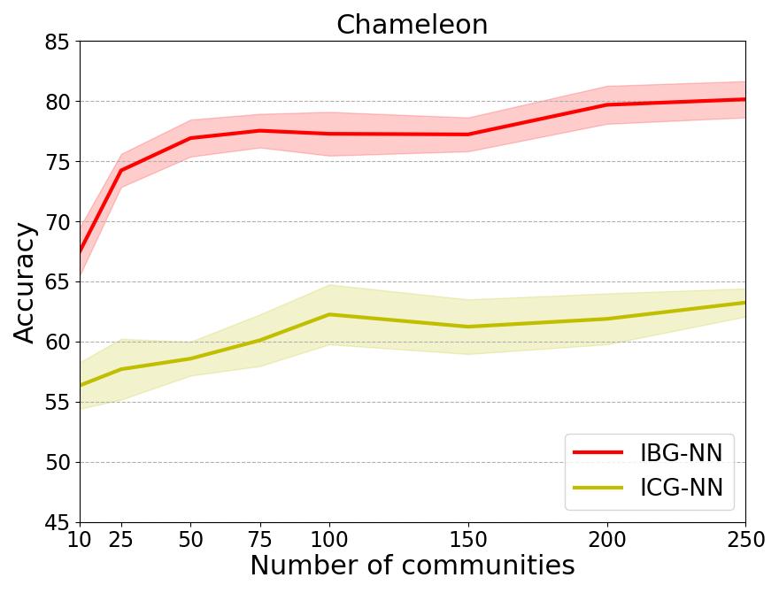
Figure 4: Accuracy of IBG-NNs and ICG-NNs on the Squirrel (left) and Chameleon (right) datasets as a function of the number of communities.

Setup.

We evaluate IBG-NN and ICG-NN on the non-sparse Squirrel and Chameleon graph [Pei et al., 2020], following the 10 data splits of Pei et al. [2020], Li et al. [2022b] and reporting the accuracy and standard deviation.

Results.

In Figure˜4, IBG-NNs exhibit significantly improved performance compared to ICG-NNs. For a small number of communities (10) on Squirrel, IBG-NNs achieve 66% accuracy, whereas ICG-NNs achieve only 45%, further demonstrating that the improvement made in IBG-NNs allowing it to reach competitive performance while being efficient. This performance gap persists across the two datasets – with IBG-NNs showing signs of further improvement as the number of communities, whereas ICG-NNs appear to have reached peak performance.

L.5 The importance of densifying

Setup.

We evaluate the effect of our proposed densifying lemma by assessing the performance of IBG-NN as a function of $\Gamma$, a parameter that controls the weight assigned to non-edges relative to edges in the IBG approximation. We explore $\Gamma$ values ranging from $0$, where weight is assigned only to existing edges, to $\frac{1-(E/N^{2})}{E/N^{2}}$, where a uniform weight of $1$ is given to each entry in the adjacency matrix. Our experiments are conducted on the large node classification graph Arxiv-Year [Lim et al., 2021] due to its low density (average degree of $6.89$).

Results.

Figure˜5 presents that the perfromance of densified IBG-NNs with $\Gamma=\frac{1-(E/N^{2})}{E/N^{2}}$ equals to that of IBG-NNs learned with standard unweighted loss, matching expectations. More importantly, Figure˜5 shows that densified IBG-NNs consistently outperform IBG-NNs learned with standard unweighted loss, across all the densification scales, validating that the theoretical improvements also translate into significant practical benefits.

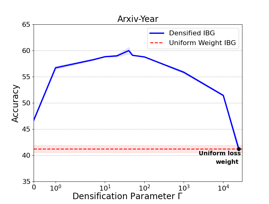
Figure 5: IBG-NN accuracy over the sparse dataset Arxiv-Year as a function of $\Gamma$. The dotted line is IBG-NN accuracy when using standard uniformly weighted loss for the IBG approximation. The rightmost point is the value of $\Gamma$ which results in a uniform cut norm under the densifying loss.

L.6 Run-time analysis

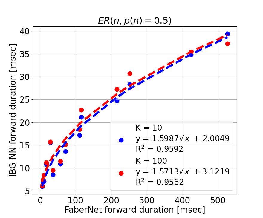
Figure 6: Runtime of K-IBG-NN as a function of DirGNN (left) and FaberNet (right) forward pass duration on $\mathrm{ER}(n,p=0.5)$ graphs for K=10, 100.

Setup.

We compare the forward pass runtimes of IBG-NN to that of the DirGNN Rossi et al. [2024] and FaberNet Koke and Cremers [2024] methods for directed graphs on Erdős-Rényi $\mathrm{ER}(n,p=0.5)$ graphs with up to $7k$ nodes. We sample $128$ node features per node, independently from $U[0,1]$. Both models use a hidden and output dimension of $128$, and $3$ layers.

Results.

Figure˜6 shows that the runtime of IBG-NN exhibits a strong square root relationship when compared to the two directed graphs methods DirGNN and FaberNet. This matches expectations, given that the time complexity of IBG-NN and message-passing neural networks are ${\mathcal{O}}(N)$ and ${\mathcal{O}}(E)$, respectively, further highlighting the difference in their efficiency.

Appendix M Choice of datasets

We present IBG-NNs, a method best suited for large graphs, capable of effectively approximating directional graphs. Consequently, our primary experiments in Section˜7.3 follow the standard graph coarsening and condensation benchmarks Reddit Hamilton et al. [2017a] and Flickr Zeng et al. [2019] where IBG-NNs demonstrates state-of-the-art performance. Additionally, IBG-NNs can be viewed as a method for handling directed graphs. To evaluate its performance in this domain, we conduct experiments on standard directed graph datasets Squirrel, Chameleon Pei et al. [2020], and Tolokers Platonov et al. [2023], where it also achieves state-of-the-art results. Finally, our graph approximation method proves particularly efficient for spatio-temporal datasets, where a fixed topology supports time-varying signals. We validate this by experimenting with IBG-NNs on the METR-LA and PEMS-BAY Li et al. [2018] datasets, where it matches the effectiveness of methods that are specifically designed for spatio-temporal data.

Appendix N Dataset statistics

The dataset statistics of the real-world directed graphs, spatio-temporal, graph coarsening and knowledge graph benchmarks used are presented below in Tables˜5, 6, 7 and 8.

Table 5: Non-sparse node classification dataset statistics.

	Squirrel	Chameleon	Tolokers
# nodes (N)	5201	2277	11758
# edges (E)	217073	36101	519000
Avg. degree ($\frac{E}{N}$)	41.71	15.85	88.28
# node features	2089	2325	10
# classes	5	5	2
Metrics	Accuracy	Accuracy	ROC AUC

Table 6: Spatio-temporal dataset statistics.

	METR-LA	PEMS-BAY
# nodes (N)	207	325
# edges (E)	1515	2369
Avg. degree ($\frac{E}{N}$)	7.32	7.29
# node features	34272	52128
Metrics	MAE	MAE

Table 7: Graph coarsening dataset statistics.

	Flickr	Reddit
# nodes (N)	89250	232965
# edges (E)	899756	114615892
Avg. degree	10.08	491.99
# node features	500	602
# classes	7	41
Metrics	Accuracy	Micro-F1

Table 8: Knowledge graph completion dataset statistics.

	Kinship	UMLS
# entities	104	135
# relations	25	46
# training triples	8544	5216
# validation triples	1068	652
# testing triples	1074	661
Avg. train. degree	82.15	38.64

Appendix O Hyperparameters

In Tables˜9, 10, 11 and 12, we report the hyper-parameters used in our real-world directed graphs, spatio-temporal, graph coarsening and knowledge graph completion benchmarks.

Table 9: Non-sparse node classification hyperparameters.

	Squirrel	Chameleon	Tolokers
# communities	50, 250	50, 250	50, 250
Encoded dim	128	128	-
$\kappa$	1	1	1
Approx. lr	0.03	0.03	0.03
Approx. epochs	10000	10000	10000
# layers	5,6,7	5,6,7	4,5,6
Hidden dim	128	128	128
Dropout	0.2	0.2	0.2
Residual connection	-	✓	✓
Jumping knowledge	Cat	Cat	Max
Normalization	True	True	True
Fit lr	0.003, 0.005	0.003, 0.005	0.003, 0.005
Fit epochs	1500	1500	1500

Table 10: Spatio-temporal node regression hyperparameters.

	METR-LA	PEMS-BAY
# communities	50	100
Encoded dim	-	-
$\kappa$	0	0
Approx. lr	0.01, 0.05	0.01, 0.05
Approx. epochs	10000	10000
# layers	5,6,7	5,6,7
Hidden dim	64, 128	64, 128
Dropout	0.0	0.0
Residual connection	✓	✓
Jumping knowledge	Max	Cat
Normalization	True	False
Fit lr	0.001, 0.003	0.001, 0.003
Fit epochs	300	300

Table 11: Graph coarsening node classification hyperparameters.

	Reddit	Flickr
# communities	50, 750	50, 750
Encoded dim	-	-
$\kappa$	0	0
Approx. lr	0.05	0.05
Approx. epochs	0	0
# layers	2, 3, 4	2, 3, 4
Hidden dim	128, 256	128, 256
Dropout	0	0
Residual connection	✓	-
Jumping knowledge	Max	Cat
Normalization	True	True
Fit lr	0.003, 0.005	0.003, 0.005
Fit epochs	1500	1500

Table 12: Knowledge graph completion hyperparameters.

	Kinship	UMLS
# communities	20	15
Encoded dim	24	48
Approx. lr	0.05	0.003
Approx. epochs	250	750
# negative samples	64	128

For our spatio-temporal experiments, we utilize the time of the day and the one-hot encoding of the day of the week as additional features, following Cini et al. [2024]. Additionaly, for spatio-temporal graphs we usually ignore the signal when fitting the IBG to the graph, but one can also concatenate random training signals and reduce their dimension to obtain one signal with low dimension $D$ to be used as the target signal for the IBG optimization.

References

- Bai et al. [2020] Lei Bai, Lina Yao, Can Li, Xianzhi Wang, and Can Wang. Adaptive graph convolutional recurrent network for traffic forecasting. In NeurIPS, 2020.
- Bianchi et al. [2020] Filippo Maria Bianchi, Daniele Grattarola, and Cesare Alippi. Spectral clustering with graph neural networks for graph pooling. In ICML, 2020.
- Bordes et al. [2013] Antoine Bordes, Nicolas Usunier, Alberto Garcia-Duran, Jason Weston, and Oksana Yakhnenko. Translating embeddings for modeling multi-relational data. In NeurIPS, volume 26, 2013.
- Borgs et al. [2008] Christian Borgs, Jennifer T Chayes, László Lovász, Vera T Sós, and Katalin Vesztergombi. Convergent sequences of dense graphs i: Subgraph frequencies, metric properties and testing. Advances in Mathematics, 2008.
- Changping et al. [2020] Wang Changping, Wang Chaokun, Wang Zheng, Ye Xiaojun, and S. Yu Philip. Edge2vec. ACM Transactions on Knowledge Discovery from Data (TKDD), 2020.
- Chen et al. [2018] Jie Chen, Tengfei Ma, and Cao Xiao. FastGCN: Fast learning with graph convolutional networks via importance sampling. In ICLR, 2018.
- Cheng et al. [2022] Kewei Cheng, Jiahao Liu, Wei Wang, and Yizhou Sun. Rlogic: Recursive logical rule learning from knowledge graphs. In KDD, 2022.
- Cheng et al. [2023] Kewei Cheng, Nesreen K Ahmed, and Yizhou Sun. Neural compositional rule learning for knowledge graph reasoning. In ICLR, 2023.
- Chien et al. [2020] Eli Chien, Jianhao Peng, Pan Li, and Olgica Milenkovic. Adaptive universal generalized pagerank graph neural network. In ICLR, 2020.
- Cini et al. [2024] Andrea Cini, Ivan Marisca, Daniele Zambon, and Cesare Alippi. Taming local effects in graph-based spatiotemporal forecasting. In NeurIPS, 2024.
- Dettmers et al. [2018] Tim Dettmers, Pasquale Minervini, Pontus Stenetorp, and Sebastian Riedel. Convolutional 2d knowledge graph embeddings. In AAAI, 2018.
- Drineas et al. [2006] Petros Drineas, Ravi Kannan, and Michael W Mahoney. Fast monte carlo algorithms for matrices i: Approximating matrix multiplication. SIAM Journal on Computing, 36(1):132–157, 2006.
- Farzaneh et al. [2015] Mahdisoltani Farzaneh, Asia Biega Joanna, and M. Suchanek Fabian. Yago3: A knowledge base from multilingual wikipedias. In CIDR, 2015.
- Fey et al. [2020] Matthias Fey, Jan-Gin Yuen, and Frank Weichert. Hierarchical inter-message passing for learning on molecular graphs. arXiv, 2020.