Neural operators struggle to learn complex PDEs in pedestrian mobility: Hughes model case study

Abstract

This paper investigates the limitations of neural operators in learning solutions for a Hughes model, a first-order hyperbolic conservation law system for crowd dynamics. The model couples a Fokker–Planck equation, representing pedestrian density, with a Hamilton–Jacobi type equation (the eikonal equation). This Hughes model belongs to the class of nonlinear hyperbolic systems which often exhibit complex solution structures, including shocks and discontinuities. In this study, we assess the performance of three state of the art neural operators Fourier Neural Operator (FNO), Wavelet Neural Operator (WNO), and Multiwavelet Neural Operator (MWT) in various challenging scenarios. Specifically, we consider (1) discontinuous and Gaussian initial conditions and (2) diverse boundary conditions while also examining the impact of different numerical schemes. Our results show that these neural operators perform well in easy scenarios characterized by fewer discontinuities in the initial condition, yet, they struggle in complex scenarios with multiple initial discontinuities and dynamic boundary condition, even when trained specifically on such complex samples. The predicted solutions often appear smoother, resulting in a reduction in total variation and a loss of important physical features. This smoothing behavior is similar to issues discussed in [1], where models that introduce artificial diffusion were shown to miss essential features such as shock waves in hyperbolic systems. This suggests that current neural operator architectures may introduce unintended regularization effects that limit their ability to capture transport dynamics governed by discontinuities. Since the Hughes model shares important structural features with models used in traffic flow, these results also raise concerns about the ability of neural operator architectures to generalize to traffic applications where shock preservation is essential.

1 Introduction

The remarkable progress in deep learning and artificial intelligence has significantly transformed computational approaches across various scientific and engineering disciplines, particularly in the context of solving partial differential equations (PDEs) [2, 3]. Traditional numerical methods, while robust and widely used, often face substantial challenges when dealing with nonlinear hyperbolic PDEs. These PDEs are characterized by complex features such as shocks, discontinuities, and steep gradients [4], which can give rise to numerical instabilities, increased computational costs, and difficulties in achieving accurate solutions. Such limitations motivate the exploration of alternative methodologies that leverage the capabilities of machine learning. One promising direction involves neural operator frameworks, which have recently shown the ability to approximate PDE solutions in a mesh-independent manner and to generalize across different instances of specific PDE problems [5, 6, 7, 8]. However, despite these advances, neural operators remain relatively unexplored in the context of nonlinear inviscid hyperbolic PDEs, particularly in realistic scenarios featuring intricate boundary conditions and solution discontinuities.

Recent work in transportation has highlighted the potential of neural operators to model complex dynamics. They have been applied to traffic flow problems [9] and traffic state estimation tasks [10, 11]. Nevertheless, challenges remain in preserving essential features of hyperbolic systems. In [1], artificial diffusion in continuum traffic models was shown to suppress key structures such as shock waves. These observations raise concerns about the ability of current neural operator architectures to generalize in systems that require accurately preserving discontinuities. In this paper, we explore how neural operators can be applied to the Hughes model, a nonlinear hyperbolic PDE system describing pedestrian dynamics through two coupled equations: a conservation law for pedestrian density and an eikonal equation governing pedestrian velocity. Owing to these coupled equations, the model naturally exhibits shocks and sharp discontinuities [12]. Originally proposed by Hughes [12] to represent pedestrian movement and evacuation in a two-dimensional space, the model has been the subject of extensive research, we refer to the survey on the numerical and analysis of the hughes model [13]. More recently, Ghattassi and N. Masmoudi [14] expanded the Hughes framework by incorporating mean-field games (MFGs) to capture pedestrian behavior that avoids high-density regions; they also investigated the stability of this generalized model [15]. Next, we introduce the mathematical Hughes model of the macroscopic pedestrian flow. The pedestrian density $\rho=\rho(t,x)$ evolves according to a scalar conservation law, and the preferred walking direction is determined by an eikonal equation. Specifically, on the interval $\Omega=(-1,1)$, the model is given by

$$\rho_{t}-\Bigl{(}\rho\,v(\rho)\,\frac{\phi_{x}}{|\phi_{x}|}\Bigr{)}_{x}=0,$$ (1a)

$$|\phi_{x}|=c(\rho),$$ (1b)

where $x\in\Omega$ is the spatial coordinate, $t\geq 0$ represents time, and $\rho(t,x)$ ranges in $[0,1]$ (interpreted as a normalized density). The cost function $c(\rho)$ is assumed to be smooth from $[0,1]$ into $[1,+\infty[$, with $c(0)=1$ and $c^{\prime}(\rho)\geq 0$. We also set the mean velocity as $v(\rho)=(1-\rho)$ and define

$$f(\rho)=\rho\,v(\rho)=\rho\,(1-\rho).$$

In many studies (see [16]), a commonly adopted choice is

$$c(\rho)=\frac{1}{v(\rho)}=\frac{1}{1-\rho}.$$ (2)

To complete the model, we prescribe an initial condition $\rho(0,\cdot)=\rho_{0}\in BV(\mathbb{R})$ and non homogeneous Dirichlet boundary data at $x=\pm 1$. Concretely, we set

$$\rho(t,-1)=\rho_{bc1}(t),\qquad\rho(t,1)=\rho_{bc2}(t),$$ (3a)

$$\phi(t,-1)=\phi_{bc1}(t),\qquad\phi(t,1)=\phi_{bc2}(t).$$ (3b)

For a discussion of more complex boundary conditions, we refer the reader to [17, 18, 13] and the references therein. Noting that (1a) can be rearranged as

$$\rho_{t}-\Bigl{(}f(\rho)\,\mathrm{sgn}(\phi_{x})\Bigr{)}_{x}=0,$$ (4)

one finds that the unique viscosity solution of the Dirichlet problem (1b), (3b) can be characterized by the value function of a control problem with the (possibly) discontinuous coefficient $c(\rho)$. In particular,

$$\phi(t,x)=\begin{cases}\displaystyle\int_{-1}^{x}c\bigl{(}\rho(t,y)\bigr{)}\,dy+\phi_{bc1}(t),&\text{if }-1\leq x\leq\xi(t),\\[6.0pt] \displaystyle\int_{x}^{\,1}c\bigl{(}\rho(t,y)\bigr{)}\,dy+\phi_{bc2}(t),&\text{if }\xi(t)\leq x\leq 1,\end{cases}$$ (5)

where $\xi(t)\in\Omega$ is implicitly determined via

$$\rho_{t}+\partial_{x}\left[\text{sgn}(x-\xi(t))\rho(1-\rho)\right]=0,$$ (6)

where $\xi(t)$ is the turning point, which can be determined by the cost integral given by

$$\int_{-1}^{\xi(t)}c\bigl{(}\rho(t,y)\bigr{)}+\phi_{bc1}(t)\ dy=\int_{\xi(t)}^{1}c\bigl{(}\rho(t,y)\bigr{)}+\phi_{bc2}(t)\ dy.$$ (7)

Obtaining smooth solutions for the Hughes model is numerically challenging due to the formation of shocks and discontinuities in crowd dynamics. These complexities necessitate robust numerical methods that can handle abrupt changes in the solution. In this work, we generate training datasets by numerically solving Eq. (6) along with Eq. (7) which balances the cumulative cost of movement toward preferred direction. The turning point, here, $\xi(t)$ represent the location at which the cost is same to move toward any direction. If the pedestrians at time $t$ happen to be in a location that is left of $\xi(t)$, they exit left and vice versa.

1.1 Neural operators: Background

Neural operators have emerged as a promising class of machine learning frameworks for approximating solution operators to partial differential equations (PDE’s). One of the earliest operator learning frameworks is DeepONet Lu et al. [3] which uses two subnetworks, a branch and a trunk network, to approximate nonlinear operators and has inspired various extensions. Following this direction, Li et al. [5] proposed the neural operator framework. One of their early models was an iterative architecture inspired by Green’s functions of elliptic PDEs involving an integral kernel which is computed by message passing on graph networks[19]. The same authors later extended this with a multipole-based design over multiscale graph structures, capturing interaction at all ranges with only linear complexity [20].

The Fourier Neural Operator (FNO) [6] marked a significant advance by learning mappings in Fourier space to capture global dependencies. It has been tested on Darcy flow (elliptic PDE with Dirichlet boundary conditions), the 2D Navier–Stokes equations with periodic boundary conditions, and the 1D viscous Burgers equation. These settings use smooth initial conditions and periodic geometries, avoiding the challenges of discontinuous, inviscid, or highly nonlinear regimes.

The Multiwavelet Neural Operator (MWT) [21] extended the idea using orthonormal multiwavelet bases, offering better localization in space and frequency. MWT was applied to the Korteweg-de Vries (KdV) equation, Burgers equation, Darcy flow, and 2D Navier–Stokes equations, generally under periodic or smoothed settings, again simplifying the solution landscape.

The Wavelet Neural Operator (WNO) [22] introduced wavelet transforms to improve localization. Tested on Darcy flow, the viscous and inviscid Burgers equations, wave advection, and the Allen–Cahn equation, WNO showed improved resolution of localized features. Yet, the configurations often involved low-amplitude or smoothed inputs, and structured grids with periodic boundaries.

The Pseudo-Differential Neural Operator (PDNO) [23] generalizes the spectral kernel of FNO by parameterizing pseudo-differential operators, improving adaptability to spatial heterogeneity. Still, PDNO has been tested mostly on smooth Darcy flow and Navier-Stokes equation with "nice" set of paramters.

Koopman Neural Operator (KNO) [24] maps nonlinear PDE dynamics to a latent linear system using Koopman theory. It has been tested on relatively simple systems like reaction-diffusion equations with smooth dynamics.

While many neural operators have demonstrated strong performance in approximating PDE solutions under smooth, periodic, or low-parameter regimes, their application to more realistic nonlinear hyperbolic PDEs with discontinuous solutions, non-periodic boundaries, or complex geometries remains limited. The use of periodic boundaries, moderate Reynolds numbers, and smoothed initial data in most benchmarks masks many of the challenges that would arise in more difficult, real-world applications. This paper investigates such limitations by testing neural operators on the Hughes model, a challenging nonlinear hyperbolic system for pedestrian dynamics where sharp fronts and solution discontinuities naturally occur.

1.2 Neural operators: Overview

Neural operators provide a framework for learning mappings between infinite-dimensional function spaces, making them well-suited for learning solutions to certain parametric partial differential equations (PDEs). They can be advantageous in scientific and engineering contexts where repeated PDE evaluations are required. Foundational works such as [6, 5] have established the theoretical and architectural underpinnings of neural operators.

Their goal is to approximate a nonlinear operator $G^{\dagger}:A\to U$, where $A=A(D;\mathbb{R}^{d_{a}})$ and $U=U(D;\mathbb{R}^{d_{u}})$ are Banach spaces of functions defined over a bounded domain $D\subset\mathbb{R}^{d}$. Given a dataset of input-output pairs $\{a_{j},u_{j}\}_{j=1}^{N}$, with $a_{j}\sim\mu$ and $u_{j}=G^{\dagger}(a_{j})$, the goal is to learn a parametric approximation $G_{\theta}:A\to U$, where $\theta\in\Theta$ belongs to a finite-dimensional parameter space. This is achieved by minimizing the expected discrepancy between predictions and ground truth:

$$\min_{\theta\in\Theta}\mathbb{E}_{a\sim\mu}\big{[}C(G(a,\theta),G^{\dagger}(a))\big{]}.$$

Neural operators are typically implemented using iterative update architectures. The input function $a\in A$ is first mapped to a feature space via a local transformation $v_{0}(x)=P(a(x))$, with $P$ often realized as a fully connected neural network. Then, for each iteration $t=0,\dots,T-1$, the representation is updated according to:

$$v_{t+1}(x):=\sigma\big{(}Wv_{t}(x)+(K(a;\phi)v_{t})(x)\big{)},\quad\forall x\in D,$$ (8)

where $W:\mathbb{R}^{d_{v}}\to\mathbb{R}^{d_{v}}$ is a learned linear operator, $\sigma$ is a non-linear activation function, and $K(a;\phi)$ is a kernel integral operator parameterized by $\phi$. The final output $v_{T}(x)$ is projected back to the target space $U$ through another local transformation $Q$.

The kernel integral operator $K(a;\phi)$ captures non-local dependencies and is defined as:

$$(K(a;\phi)v_{t})(x):=\int_{D}\kappa(x,y,a(x),a(y);\phi)v_{t}(y)\,dy,\quad\forall x\in D,$$ (9)

where $\kappa:\mathbb{R}^{2(d+d_{a})}\to\mathbb{R}^{d_{v}\times d_{v}}$ is a learnable kernel function. This construction extends classical neural network operations to infinite-dimensional spaces via compositions of integral operators and pointwise nonlinearities.

Each neural operator computes (9) differently, trying to achieve a desired accuracy while reducing computational time. For instance, the Fourier neural operator imposes the restriction $\kappa(x,y,a(x),a(y);\phi)=\kappa(x-y;\phi)$, converting the kernel integral operator into a convolution operator. This structure allows fast computation using the Fast Fourier Transform (FFT) (see figure 1). Indeed, by the convolution theorem, we have:

$$(f*g)(x)=\mathcal{F}^{-1}(\mathcal{F}(f)\cdot\mathcal{F}(g))(x).$$

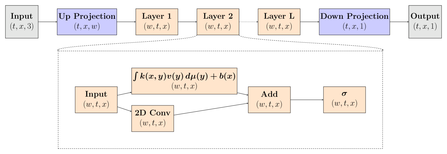
Figure 1: Layer-wise architecture of Neural Operator.

Figure 1 illustrates the data processing pipeline of a neural operator (NO). The NO accepts input with shape $(t,x,3)$, meaning that for each $(t,x)$ pair, there are three values corresponding to the input variable, the time coordinate, and the space coordinate. This input is first projected into a higher-dimensional space, increasing the feature dimension from 3 to a width $w$ (with $w>3$). The resulting representation is then permuted to the shape $(w,t,x)$ and then processed through multiple operator layers. The output of the last operator layer $L$ is then permuted again to $(t,x,w)$ and finally down-projected to produce an output with shape $(t,x,1)$, so that each $(t,x)$ pair corresponds to a single output value.

To systematically examine the capabilities and limitations of neural operators, we perform extensive numerical experiments using three state-of-the-art neural operator architectures: Fourier Neural Operator (FNO) [6], Wavelet Neural Operator (WNO)[22], and Multiwavelet Neural Operator (MWNO) [21]. Our evaluation encompasses various scenarios, including multiple discontinuous initial conditions, different boundary conditions and two different numerical schemes. Through these rigorous tests, we identify strengths and reveal important shortcomings of neural operators when handling complex nonlinear hyperbolic PDEs such as the Hughes model.

The numerical experiments demonstrate that although neural operators effectively approximate solutions under simpler conditions, their performance substantially deteriorates when confronted with realistic complexities inherent to pedestrian dynamics modeling. Thus, this study highlights the need for developing enhanced neural operator architectures or refined training strategies, supporting further advancement in machine learning for complex nonlinear hyperbolic systems.

The rest of this paper is structured as follows: Section 2 provides a comprehensive literature review of relevant studies on neural operators and their applications to PDEs, particularly nonlinear hyperbolic equations. Section 3 provides a comprehensive description of the Hughes model and outlines the common numerical methods used for its solution. In Section 4, we present detailed formulations and technical insights into the neural operator architectures: FNO, WNO, and MWT. Section 5 describes the experimental setup and discusses the results obtained from testing the neural operators under various challenging conditions. Finally, Section 6 concludes the paper and outlines potential directions for future research.

2 Numerical schemes for Hughes model

Due to the inherent complexity of the Hughes model, conventional numerical approaches often require fine discretization and substantial computational effort, for more details we refer to [18, 25, 26, 27] and references therein. To address these challenges, we employ both the wavefront tracking algorithm (WFT) [18] and an adapted finite volume scheme (Godunov) [28] to compute the solution. The wavefront tracking algorithm constructs piecewise-constant approximations and precisely tracks the evolution of discontinuities, making it particularly effective for capturing the hyperbolic structure of the governing equations with minimal numerical diffusion. Moreover, the Godunov scheme, situated within the finite-volume framework, solves localized Riemann problems at each cell interface, ensuring robust treatment of shocks and other nonlinear wave interactions. By coupling these two techniques, we gain a comprehensive perspective that not only facilitates cross-verification but also exploits the complementary strengths of each method—wavefront tracking’s refined handling of discontinuities and Godunov’s well-established stability in flux computations to produce more accurate and reliable solutions. In the following subsections, we explore the wavefront tracking algorithm in detail and subsequently discuss the Godunov scheme, providing further justification for employing both approaches in tandem.

2.1 Wave-front tracking scheme [18]

The wave–front tracking technique for classical scalar conservation laws constructs piecewise constant exact solutions of an approximated problem with piecewise constant initial data and a piecewise linear flux $f_{\epsilon}$, where $f_{\epsilon}(\rho)=f(\rho)=\rho\,v(\rho),$ with $v(\rho)$ the speed, on the mesh $M_{\epsilon}=\{\rho_{i}^{\epsilon}\}_{i=0}^{2^{\epsilon}}\subset\Omega,$ with $\Omega=[0,1]$ as

$$M_{\epsilon}=2^{-\epsilon}\mathbb{N}\cap[0,1].$$ (10)

Initialization. Approximate the initial datum $\rho_{0}$ by a piecewise constant function

$$\rho_{0}^{\epsilon}(x)=\sum_{j\in\mathbb{Z}}\rho_{0,j}^{\epsilon}\,\chi_{]x_{j-1},x_{j}]},$$ (11)

with $\rho_{0,j}^{\epsilon}\in M_{\epsilon}$, chosen so that

$$\lim_{\epsilon\to\infty}\|\rho_{0}^{\epsilon}-\rho_{0}\|_{L^{1}(\Omega)}=0,\quad\text{and}\quad\operatorname{TV}(\rho_{0}^{\epsilon})\leq\operatorname{TV}(\rho_{0}).$$ (12)

Here, $\operatorname{TV}(g)$ denotes the total variation of any bounded variation function $g$ over the interval $\Omega=[0,1]$, defined as

$$\operatorname{TV}(g)=\sup_{\mathcal{P}}\sum_{j}\left|g(x_{j})-g(x_{j-1})\right|,$$

where the supremum is taken over all finite partitions $\mathcal{P}$ of the interval. Intuitively, total variation measures the cumulative size of the jumps in g. The points $x_{j}^{\prime}s$ are not necessarily on a uniform grid; refinement is done on the density mesh $M_{\epsilon}$.

Set $x_{0}=\xi_{0}$, where $\xi_{0}$ satisfies the cost balance equation at $t=0$:

$$\int_{-1}^{\xi_{0}}c\bigl{(}\rho_{0}^{\epsilon}(y)\bigr{)}\,dy=\int_{\xi_{0}}^{1}c\bigl{(}\rho_{0}^{\epsilon}(y)\bigr{)}\,dy.$$ (13)

In piecewise form:

$$\sum_{j\leq 0}c(\rho_{0,j}^{\epsilon})(x_{j}-x_{j-1})=\sum_{j>0}c(\rho_{0,j}^{\epsilon})(x_{j}-x_{j-1}).$$ (14)

For small $t>0$, construct $(\rho^{\epsilon},\xi_{\epsilon})$ to approximate the coupled problem (1) by solving local Riemann problems:

$$\begin{cases}\partial_{t}\rho+\partial_{x}\Bigl{(}\operatorname{sgn}(x-\xi_{0})f^{\epsilon}(\rho)\Bigr{)}=0,\\[2.84526pt] \rho(0,x)=\begin{cases}\rho_{0,0}^{\epsilon}\quad\text{if }x<\xi_{0},\\[2.84526pt] \rho_{0,1}^{\epsilon}\quad\text{if }x>\xi_{0},\end{cases}\\[2.84526pt] \dot{\xi}(\rho^{+}-\rho^{-})=\Psi[\rho],\end{cases}$$ (15)

$$\begin{cases}\partial_{t}\rho+\partial_{x}\Bigl{(}\operatorname{sgn}(x_{j}-\xi_{0})f^{\epsilon}(\rho)\Bigr{)}=0,\\[2.84526pt] \rho(0,x)=\begin{cases}\rho_{0,j}^{\epsilon}\quad\text{if }x<x_{j},\\[2.84526pt] \rho_{0,j+1}^{\epsilon}\quad\text{if }x>x_{j},\end{cases}\\[2.84526pt] j\neq 0.\end{cases}$$ (16)

where,

$$\left\{\int_{\bar{\xi}+\delta}^{1}-\int_{-1}^{\bar{\xi}-\delta}\right\}\partial_{t}\bigl{[}c(\rho(t,y))\bigr{]}\,dy=:\Psi.$$ (17)

Here, $\bar{\xi}$ denotes the turning point at a fixed time, $\delta>0$ is a small constant that defines a buffer around $\bar{\xi}$, and $\Psi$ represents the net time variation of the cost across the buffer region.

Furthermore,

$$\rho^{+}(t)=\rho(t,\xi(t)^{+})\quad\text{and}\quad\rho^{-}(t)=\rho(t,\xi(t)^{-})$$ (18)

are the right and left traces of $\rho$ at $x=\xi(t)$.

Solving the Riemann problems above replaces smooth rarefaction fronts by fans of constant values $\rho_{1,j}^{\epsilon}$, $j=l_{1},\cdots,l_{N_{\epsilon}}$ such that

$$|\rho_{1,j}^{\epsilon}-\rho_{1,j-1}^{\epsilon}|=2^{-\epsilon},$$ (19)

separated by discontinuities with speeds

$$\lambda_{1,j}=-\,\operatorname{sgn}(\phi_{x})\bigl{(}1-\rho_{1,j}^{\epsilon}-\rho_{1,j-1}^{\epsilon}\bigr{)}.$$ (20)

For the turning curve, use the Riemann solver given in Section 3 of [18] (with $\rho_{M}$ approximated by the closest point in $M_{\epsilon}$). The resulting new densities (if any) are inserted between the original states and relabeled as $\rho_{1,j}^{\epsilon}$. Each pair of consecutive states is given a wave speed $\lambda_{1,j}$ or $\dot{\xi}_{\epsilon}$, with associated departure point $x_{j}$. Hence, we get the wave trajectories as:

$$x_{j}(t)=x_{j}+\lambda_{1,j}\,t,\quad x_{0}(t)=\xi_{\epsilon}(t)=\xi_{0}+\dot{\xi}_{\epsilon}\,t,$$ (21)

and to update the solution for small $t>0$

$$\rho^{\epsilon}(t,\cdot)=\sum_{j\in\mathbb{Z}}\rho_{1,j}^{\epsilon}\,\chi_{]x_{j-1}(t),\,x_{j}(t)]}.$$ (22)

The piecewise constant approximate solution $\rho^{\epsilon}$ constructed in the previous time step is extended until the first instance when either two waves interact or a wave encounters the turning curve $\xi^{\epsilon}$. In both scenarios, the intermediate state is removed, and a new Riemann problem is formulated. Its solution is computed using the Reimann solver described in Section 3 of [18] when the turning curve is reached, which permits further extension of $\rho^{\epsilon}$ and $\xi_{\epsilon}$ up to the subsequent interaction event. The absorbing boundary conditions are implemented by simply discarding any waves that strike the left or right boundaries. An illustration of an example solution can be seen in figure 2(b). The MATLAB code used for the above scheme can be found at http://www-sop.inria.fr/members/Paola.Goatin/wft.html.

2.2 Godunov scheme

Godunov scheme is a numerical method used for solving hyperbolic conservation laws. This finite volume approach leverages approximate solutions of the Riemann problem at cell interfaces to capture discontinuities.

This section discusses the numerical solutions of (1) using the Godunov scheme [28]. For a conservation law of type $u_{t}+F(u)_{x}=0$, the Godunov flux is

$$h(u,v)=F\bigl{(}R(0;u,v)\bigr{)},$$

where $R(0;u,v)$ is the solution of the Riemann problem with left and right states $u$ and $v$ evaluated at $x=0$. At each time step:

1. Given $\rho(t=0,x)=\rho_{0}(x)$, determine the turning point $\xi(t)$ by using equation (7) using the method outlined in the Appendix (Section 6.2), rather than the Fast Sweeping algorithm discussed in [29].

2. Given $\xi(t)$, Solve the nonlinear conservation law (6) using the Godunov scheme.

Let $[-1,1]$ be divided into $N$ uniform cells $I_{j}=[x_{j-\tfrac{1}{2}},x_{j+\tfrac{1}{2}}]$ with centers $x_{j}=j\Delta x$, $\Delta x=2/N$ and $\Delta t^{n}=t^{n+1}-t^{n}$. The Godunov (numerical) fluxes are computed as:

$$q^{n-1}_{j+1/2}\;=\;F\bigl{(}\rho^{n-1}_{j},\,\rho^{n-1}_{j+1})\bigr{.}.$$ (23)

The density is updated via

$$\rho^{n}_{j}=\rho^{n-1}_{j}-\frac{\Delta t^{n-1}}{\Delta x}\,\bigl{(}q^{n-1}_{j+1/2}-q^{n-1}_{j-1/2}\bigr{)}.$$ (24)

The flux function is given by:

$$F(\rho^{n-1}_{j},\rho^{n-1}_{j+1})=\begin{cases}\rho^{n-1}_{j}\,(1-\rho^{n-1}_{j}),&\text{if }\rho^{n-1}_{j+1}\leq\rho_{cr}\text{ and }\rho^{n-1}_{j}\leq\rho_{cr},\\[2.84526pt] q_{max},&\text{if }\rho^{n-1}_{j+1}\leq\rho_{cr}\text{ and }\rho^{n-1}_{j}>\rho_{cr},\\[2.84526pt] \min\Bigl{\{}\rho^{n-1}_{j+1}\,(1-\rho^{n-1}_{j+1}),\,\rho^{n-1}_{j}\,(1-\rho^{n-1}_{j})\Bigr{\}},&\text{if }\rho^{n-1}_{j+1}>\rho_{cr}\text{ and }k_{xup}\leq\rho_{cr},\\[2.84526pt] \rho^{n-1}_{j+1}\,(1-\rho^{n-1}_{j+1}),&\text{if }\rho^{n-1}_{j+1}>\rho_{cr}\text{ and }\rho^{n-1}_{j}>\rho_{cr}.\end{cases}$$

Here $q_{max}=1$ and $\rho_{cr}=1/2$. Now, update for each time step $t<T$. The resulting function $\rho(x,t)$ is then the Godunov approximation of the Hughes model’s solution. An illustration of an example solution can be seen in figure 2(c).

(a) Crowd Illustration

(b) WFT algorithm simulation

(c) Godunov scheme simulation

Figure 2: Illustration of Hughes pedestrian dynamics*
*High discretization used here for better visualization

2.3 Data generation

The quality of the data is critical in the domain of operator learning. To rigorously assess the influence of data quality on the performance of neural operators, both training and testing datasets are generated using the numerical schemes detailed previously. In both approaches, the initial conditions (here, initial density profiles $\rho(0,x)$) and/or boundary conditions are provided as an input to compute the solution $\rho(t,x)$ over the entire space-time grid. In this subsection, we present the procedure we follow to generate the different datasets that will be used for training and testing the neural operators.

2.3.1 Generate initial conditions

Two types of initial conditions are used to probe different dynamical regimes of the Hughes model. Firstly, the piecewise constant initial condition which introduces discontinuities in the initial density profiles. These abrupt density jumps can create shocks and lead to complex interactions in pedestrian flow. Secondly, the Gaussian initial condition, as they provide a smooth, continuous initial density profiles without discontinuities. It serves to isolate the effects of the boundary conditions on the evolution of the flow. The precise methodologies for constructing both the piecewise constant and Gaussian initial conditions are described below.

Piecewise constant initial conditions:

The generation of the initial density profiles $\rho(t=0,x)$ is carried out in two main steps. First, $N+1$ density values are generated, where $N$ denotes the number of discontinuities in the initial condition. These values are then used to construct a piecewise constant (step) function over the spatial domain $[x_{1},x_{n}]$. The first value, $k_{1}$, is sampled from a uniform distribution on the interval $[0.05,0.95]$. For each subsequent index $j=2,\dots,N+1$, the value $k_{j}$ is computed by adding a random increment $\delta_{j}\sim\mathcal{N}(0,0.5)$ to $k_{j-1}$. Each $k_{j}$ is adjusted, if necessary, to ensure it satisfies the constraints $0<k_{j}<1$ and $k_{j}\neq k_{j-1}$.

In the second step, $N$ unique positions $s_{i}$ are sampled uniformly from $[x_{1},x_{n}]$. These positions are then sorted in ascending order, partitioning the spatial domain into $N+1$ contiguous regions:

$$r_{1}=[x_{1},s_{1}),\quad r_{2}=[s_{1},s_{2}),\quad\dots,\quad r_{N}=[s_{N-1},s_{N}),\quad r_{N+1}=[s_{N},x_{n}].$$

Each density value $k_{j}$ is assigned to its corresponding sub-interval, producing constant-density regions: $\rho_{r_{1}}=k_{1},\ \rho_{r_{2}}=k_{2},\ \dots,\ \rho_{r_{N+1}}=k_{N+1}$. This procedure is applied to generate the datasets used in both Problem I and Problem II in Subsection  3.3. Representative examples of these initial conditions are provided in Figure 3. The hyperparameters used in the Godunov scheme and wavefront-tracking algorithm are listed in Table 1. Meanwhile, Figure 4 illustrates how the same initial condition evolves under both solvers, highlighting the resulting density profile $\rho(t,x)$.

Gaussian initial condition:

The spatial domain $[x_{1},x_{n}]$ is initialized with a continuous Gaussian pulse to ensure a smooth initial density profile. The profile is defined by a Gaussian function whose parameters are randomly sampled as follows:

$$\mu\sim\mathcal{U}(0,x_{n}),\quad\sigma\sim\mathcal{U}\left(0,\frac{x_{n}}{2}\right),$$

where $\mu$ denotes the mean and $\sigma$ the standard deviation of the Gaussian. The initial density is then given by

$$\rho(t=0,x)=\exp\left(-\frac{(x-\mu)^{2}}{2\sigma^{2}}\right).$$

This procedure is used to generate the initial density profiles for the data used in Problem III in Subsection 3.3.

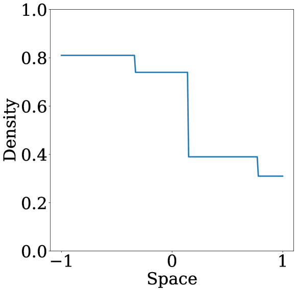
(a) Three discontinuities

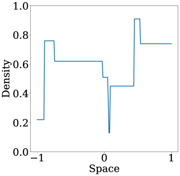
(b) Seven discontinuities

(c) Nine discontinuities

Figure 3: Example data for initial conditions with multiple discontinuities

Table 1: Simulation parameters for Godunov scheme and WFT algorithm

Parameter	Godunov Scheme	WFT Algorithm
Domain $x$	$[-1,1]$	$[-1,1]$
Time interval $t$	$[0,3]$	$[0,3]$
Spatial resolution $\Delta x$	$1/500$	$2/201$
Temporal resolution $\Delta t$	$1/600$	$1/2000$
Maximum density $\rho_{\max}$	$1$	1
Maximum velocity $v_{\max}$	$1$	1
Critical density $\rho_{\text{cr}}$	$1/2$	–
Maximum flow $q_{\max}$	$1/4$	–
Mesh size $\Delta\rho$	–	$1/250$

2.3.2 Generate boundary conditions

The flow at the boundaries is regulated via the potential function $\phi(t,x)$ (see equation (3b)), with pedestrians naturally moving from regions of high to low potential. In this study, we consider three distinct scenarios for the boundary conditions. In Problem I in Subsection 3.3, pedestrians are allowed to exit the domain freely by setting:

$$\phi(t,-1)=\phi_{bc1}(t)=0,\qquad\phi(t,1)=\phi_{bc2}(t)=0.$$ (25a)

In the second scenario in Problem II in Subsection 3.3, high potential values are imposed near $x=\pm 1$ to create a repulsive effect that directs pedestrians away from the exits and into the interior of the domain, modeling their behavior at the closed exits.

$$\phi(t,-1)=\phi_{bc1}(t)=10000,\qquad\phi(t,1)=\phi_{bc2}(t)=10000.$$ (26a)

Finally, a third scenario in Problem III in Subsection 3.3, features time-varying boundary conditions, where the value of $\phi(t,x)$ at $x=-1$ is varied with time as follows.

$$\phi(t,-1)=\phi_{bc1}(t) =\begin{cases}10000,&0\leq t<t_{1},\quad t_{1}\sim\mathcal{U}(0.08,0.5),\\[2.84526pt] 0,&t_{1}\leq t<t_{2},\quad t_{2}\sim\mathcal{U}(0.8,1),\\[2.84526pt] 10000,&t_{2}\leq t<t_{3},\quad t_{3}\sim\mathcal{U}(1.4,2.2),\\[2.84526pt] 0,&t_{3}\leq t<t_{4},\quad t_{4}\sim\mathcal{U}(2.5,2.75),\\[2.84526pt] 10000,&t_{4}\leq t<t_{5},\quad t_{5}\sim\mathcal{U}(2.8,3.33),\\[2.84526pt] 0,&t_{5}\leq t<5,\end{cases}$$ (27a)

$$\phi(t,1)=\phi_{bc2}(t) =0,\quad\forall\,t\in[0,5].$$

2.3.3 Generate dataset for various test scenarios

The methodology used to generate the dataset for neural operators for different test scenarios is as follows: For Problem I given in Subsection 3.3, for both the numerical methods, two datasets are produced, classified as easy and complex. Easy samples are defined as those for which the difference between the maximum and minimum turning point ($\Delta\xi=\xi_{\text{max}}-\xi_{\text{min}}$) is less than 0.3, having up to three discontinuities in their initial density profile ($N\leq 3$, where, $N$ = number of discontinuities in the initial density profile). In contrast, complex samples are characterized by a turning point difference greater than 0.3 ($\Delta\xi>0.3$), having one to ten discontinuities in their initial density profile ($N\leq 10$). This choice of $\Delta\xi$ is supported by our observation that as $\Delta\xi$ increases, the system becomes more complex. Consequently, complex samples display a higher degree of variability in turning points and more pronounced discontinuities in their initial density profile, leading to more intricate patterns in the solution $\rho(t,x)$. For the easy samples ($\Delta\xi<0.3\text{ and }N\leq 3$), $\rho(t=0,x)$ follows the same distribution with parameters as shown in section 2.3.1 for both the methods, which means, the data generated from the two numerical methods may not be exactly similar but share a common distribution. For the complex samples ($\Delta\xi>0.3\text{ and }N\leq 10$), $\rho(t=0,x)$ are generated once. Then, these same initial conditions are used to generate solution $\rho(t,x)$, using both the numerical methods to get a fair comparison. The boundary conditions used for both easy and complex samples are same and are given by equation (25). Figure 4 shows an example of a sample generated by the Godunov scheme and the WFT algorithm for the same $\rho(t=0,x)$.

For Problem II described in Subsection 3.3, samples feature initial conditions with up to three discontinuities only. The corresponding boundary conditions for this case are different from Problem I and are provided in equation (26). Moreover, the data for this scenario is generated exclusively using the Godunov scheme.

For Problem III described in Subsection 3.3, Gaussian initial conditions are employed. Specifically, the initial density profile $\rho(0,x)$ follows a Gaussian distribution (see Subsection 2.3.1). This problem is further subdivided into two cases based on the boundary conditions: (i) boundary conditions as given in equation (25), and (ii) boundary conditions as given in equation (27). The data for both cases are generated exclusively using the Godunov scheme.

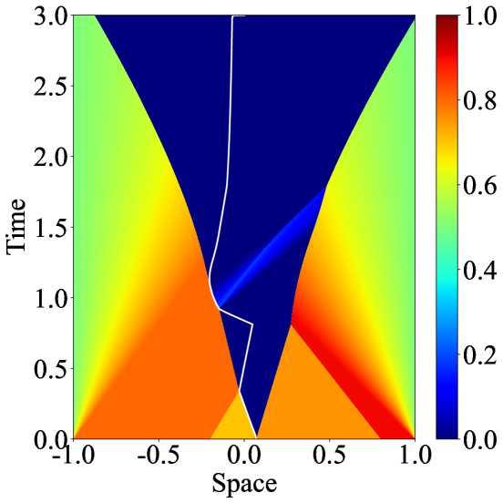
(a) Data Generated by Godunov Scheme

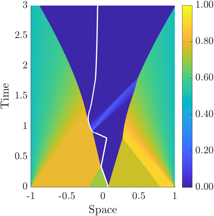
(b) Data Generated by WFT Algorithm

Figure 4: Example data for Godunov and WFT scheme, with same initial condition*
*High discretization used here for better visualization

2.3.4 Data preprocessing

The dataset for the Godunov scheme and the WFT algorithm is generated using the hyperparameters shown in Table 1. Each dataset is down sampled to reduce computational cost while preserving essential solution features. For the Godunov scheme, each raw sample is initially generated with a spatiotemporal resolution of $(x=1000,t=1800)$, down sampled to a shape of $(x=200,t=50)$, which is used for training the FNO and WNO.

In contrast, the sample generated via the WFT algorithm is of shape $(x=201,t=6000)$, which is then down sampled to $(x=201,t=50)$. This choice of generating data at $x=201$ is deliberate, as WFT inherently produces stair-step data due to its discontinuous structure, and retaining full spatial resolution is necessary to accurately capture the locations of discontinuities at each time step. Since using $201$ points between $[-1,1]$ gives a discretization of $0.01$, it becomes easier to round the values to 2 decimal places to preserve the location of discontinuities.

For the multi-wavelet neural operator, which requires square input domains due to the structure of multi-wavelet transforms, the samples from both numerical methods are uniformly down sampled to a resolution of $(128,128)$.

Each sample is divided into two components: the training input $X$ and the target output $Y$. For problems I and II in Subsection 3.3, the input $X$ consists of the initial condition $\rho(0,x)$ embedded into a tensor with the same dimensions as the full spatiotemporal grid, with all values for $t>0$ set to zero (see Figure 5(b)). Problem III, described in Subsection 3.3, is divided into two subproblems. In the first sub-problem, the initial value problem, the input $X$ is constructed in the same manner as in the other cases (see Figure 5(b)). In the second sub-problem, the mixed initial boundary value problem, the input $X$ includes both the initial condition and the boundary conditions, while all other values of $\rho(t,x)$ for $t>0$ and $-1<x<1$ are set to zero (see Figure 6(a)). In every case, the target output $Y$ comprises the complete solution trajectory $\rho(t,x)$ (see Figures 5(c) and 6(b)).

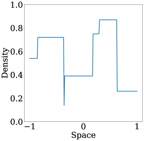
(a) Initial Condition

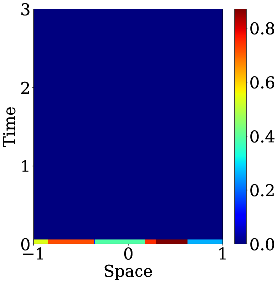
(b) Training Input (X)

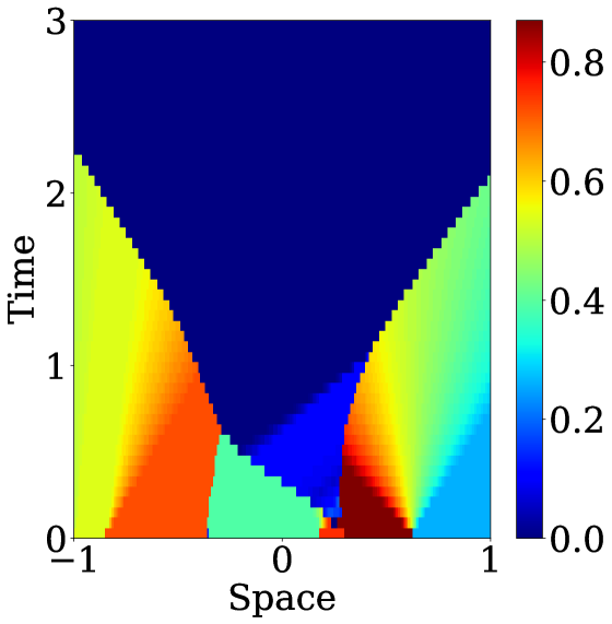
(c) Target Output (Y)

Figure 5: Training data for initial value problem

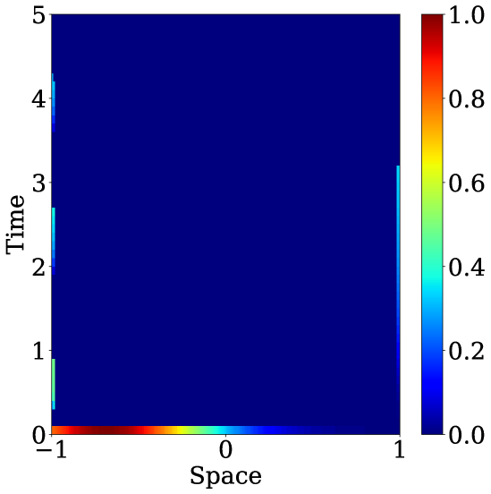
(a) Training Input (X)

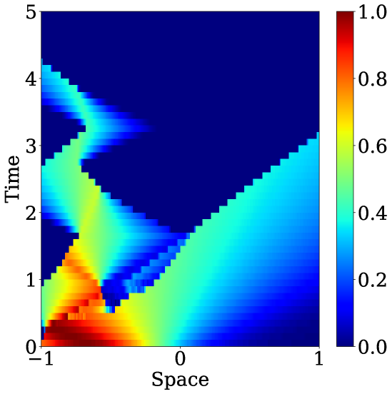
(b) Target Output (Y)

Figure 6: Training data for mixed initial-boundary value problem

3 Experiments and results

This section presents the experimental setup and evaluation of the neural operators across the different test scenarios. The first subsection defines the metric used for evaluation of the neural operators. Subsequent subsections detail the quantitative and qualitative results obtained from the experiments.

3.1 Model evaluation

For both training and evaluation, the relative $L_{2}$ loss is used as the primary error metric. This loss function measures the deviation between the predicted solution and the ground truth, normalized by the magnitude of the ground truth itself. It is defined as:

$$\text{Data Loss}=\min_{\Theta}\frac{1}{|\mathcal{D}|}\sum_{i\in\mathcal{I}}\left\|\mathcal{L}(G_{\Theta}(\mathbf{X}(i)),\mathbf{Y}(i))\right\|_{2}^{2},$$ (28)

where $\Theta$ denotes the trainable parameters of the neural operator, $\mathcal{D}$ is the dataset, $\mathcal{I}$ is the index set of training samples, and $G_{\Theta}(\mathbf{X}(i))$ is the model’s prediction for the input $\mathbf{X}(i)$. The function $\mathcal{L}(\cdot,\cdot)$ computes the relative error between the predicted and true solution fields:

$$\mathcal{L}(\hat{\mathbf{Y}},\mathbf{Y})=\frac{\left\|\hat{\mathbf{Y}}-\mathbf{Y}\right\|_{2}}{\left\|\mathbf{Y}\right\|_{2}},$$ (29)

where $\hat{\mathbf{Y}}$ is the predicted solution and $\mathbf{Y}$ is the ground truth.

By normalizing the error, this metric ensures that all samples contribute equally to the overall loss, regardless of their absolute scale. It also allows for meaningful comparison of model performance across datasets with different dynamics or initial conditions. This relative error metric is used consistently across all neural operators (Fourier neural operator (FNO), wavelet neural operator (WNO), and multiwavelet neural operator (MWNO)) and all data variants (Godunov/WFT, easy/complex), allowing for fair and robust comparison of performance across architectures and scenarios.

3.2 Total variation-based diffusion metrics

While the relative $L^{2}$ error captures global approximation accuracy, it does not reflect how well the model preserves physical features such as discontinuities. To address this, we introduce secondary metrics based on the total variation (TV) of the solution, which are sensitive particularly to diffusion. Total variation provides a global measure of how much the solution varies across space, making it informative for transport-dominated problems.

Given a fixed sample and a solution profile $\rho_{j}^{n}$ at time step $n\in\{0,\dots,T\}$ and spatial grid index $j$, the discrete total variation is defined as:

$$\operatorname{TV}(u^{n})=\sum_{j=1}^{N-1}\left|\rho_{j+1}^{n}-\rho_{j}^{n}\right|.$$

For any sample $m\in\{1,\dots,M\}$ and time step $n$, we denote the TV difference by

$$\delta_{\mathrm{TV}}^{n,m}=\operatorname{TV}(\rho^{n,m})-\operatorname{TV}(\hat{\rho}^{n,m}),$$

where $\rho^{n,m}$ and $\hat{\rho}^{n,m}$ denote the ground truth and predicted solutions, respectively. Positive values of $\delta_{\mathrm{TV}}^{n,m}$ indicate that the predicted solution has less total variation than the reference, which may be due to smoothing of discontinuities, damping of valid oscillations, or flattening of variable regions. Negative values, on the other hand, may reflect excess variation introduced by oscillations or artificial steepness (over-sharpening).

While the signed metric captures both under- and over-variation, our focus is on identifying smoothing behavior. Therefore, we compute the "clipped TV" loss as:

$$\overline{\delta}_{\mathrm{TV}}^{+}=\frac{1}{MT}\sum_{m=1}^{M}\sum_{n=1}^{T}\max\left(0,\delta_{\mathrm{TV}}^{n,m}\right),$$

which isolates cases where the predicted solution underestimates total variation. This provides a more targeted view of potential diffusive effects in the model.

3.3 Numerical experiments and results

To systematically evaluate the performance and generalization capabilities of neural operators, a series of experiments are designed. These experiments involve various initial and boundary conditions. The experimental setup consists of the following three problems.

3.3.1 Problem I

We begin the evaluation by testing FNO, WNO and MWNO on the datasets described in Subsection 2.3.4 (see also Figure 5). Each of these three neural operators are trained and tested on both easy and complex datasets generated independently by the Godunov scheme and the Wavefront Tracking (WFT) algorithm. This setup enables a comprehensive comparison of operator performance across varying levels of difficulty and over different numerical solvers.

The primary goal is to assess not only how each operator handles increasing complexity in the initial conditions, but also whether there is any marked difference in learning patterns between data produced by the Godunov scheme and the WFT algorithm. The hyperparameter for all three operators are summarized in Table 6.

Tables 2 and 3 present the relative $L_{2}$ loss for the experiments carried out on the IVP using the data generated by the WFT algorithm and the Godunov scheme, respectively. In particular, the Godunov scheme exhibits a superior learning capacity compared to the WFT algorithm. For comparison, Figures 7 and 8 show the sample for the same initial condition. But, the relative $L_{2}$ loss for the given sample using Godunov scheme is $0.173$ while for the WFT algorithm it is $0.215$. This shows how FNO performs very poorly irrespective of the training data.

Table 2: Relative $L_{2}$ loss for data generated using WFT Algorithm $(\Delta\rho=1/250)$

Data	Num_Sample		FNO		MWT		WNO
	Easy	complex	Easy	complex	Easy	complex	Easy	complex
Train	2960	8040	0.038	0.094	0.047	0.091	0.060	0.109
Val	880	2400	0.078	0.126	0.085	0.127	0.076	0.126
Test	880	2400	0.078	0.127	0.085	0.128	$\mathbf{0.076}$	$\mathbf{0.126}$
Time per Epoch (s)			$\mathbf{6.91}$	$\mathbf{18.78}$	13.54	29.48	42.98	111.34

Table 3: Relative $L_{2}$ loss for data generated using Godunov Scheme

Data	Num_Sample		FNO		MWT		WNO
	Easy	complex	Easy	complex	Easy	complex	Easy	complex
Train	3000	8040	0.022	0.081	0.034	0.088	0.023	0.097
Val	900	2400	0.064	0.113	0.071	0.118	0.064	0.113
Test	900	2400	0.064	0.114	0.070	0.119	$\mathbf{0.063}$	$\mathbf{0.113}$
Time per Epoch (s)			$\mathbf{5.04}$	$\mathbf{14.56}$	10.98	35.47	42.46	119.45

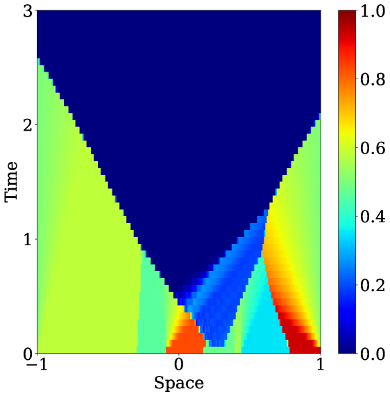
(a) Real Data

(b) Predicted Data

Figure 7: Prediction results for data with six discontinuities in initial condition, generated using Godunov Scheme and trained on FNO

(a) Real Data

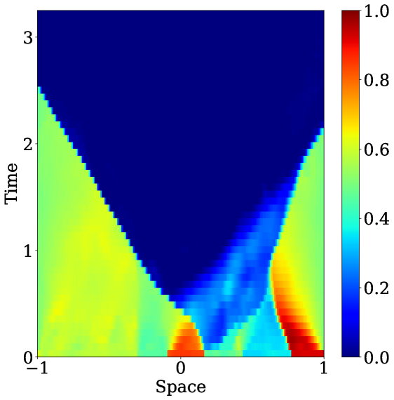
(b) Predicted Data

Figure 8: Prediction results for data with six discontinuities in initial condition, generated using WFT algorithm and trained on FNO

It is possible that the mesh size $\Delta\rho$ plays a key role in the observed failure of the learning process for the WFT algorithm. The mesh size $\Delta\rho=1/250$ used to generate the data used in Table 2 causes numerical instability for some samples. This numerical instability can be quantified by the "cost integral balance error" as follows.

$$E_{\text{cost}}=\max_{t}\left|\int_{-1}^{\xi(t)}\frac{1}{1-\rho(t,y)}\,dy-\int_{\xi(t)}^{1}\frac{1}{1-\rho(t,y)}\,dy\right|.$$ (30)

For example, Figure 9 shows the same sample generated by the Godunov and WFT scheme. Specifically, the sample depicted in Figure 9(b), generated with $\Delta\rho=1/250$, exhibits numerical instability with $E_{\text{cost}}$ tending to infinity, consequently producing an unrealistic solution.. This shows the inconsistency in the data produced by the WFT algorithm, as compared to the Godunov scheme, leading to high relative $L_{2}$ loss.

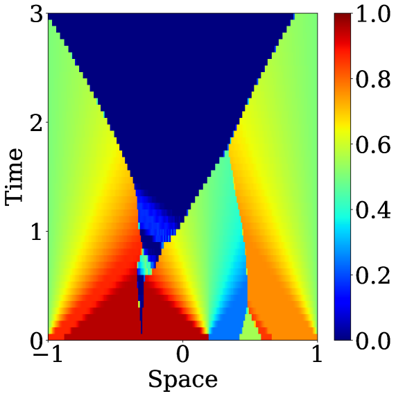
(a) Godunov Scheme

(b) WFT with $\Delta\rho=1/250$

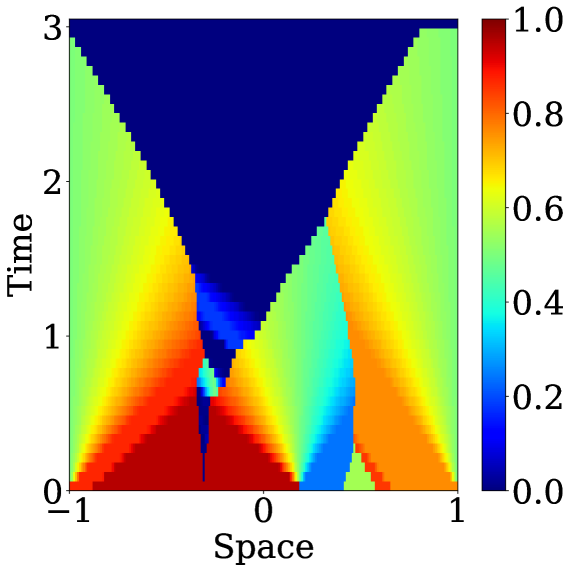
(c) WFT with $\Delta\rho=1/800$

Figure 9: Sample comparison for Goudnov and WFT algorithm

Therefore, additional experiments were conducted using data generated by the WFT algorithm with $\Delta\rho=1/800$ and with samples having $E_{\text{cost}}<0.1$. Figure 9(c) illustrates that this approach yields a more accurate solution, which can potentially reduce the relative $L_{2}$ loss. The results of this experiment are presented in Figure 10(a), where the relative $L_{2}$ loss is plotted against the number of discontinuities in the initial condition. It shows that even after significantly increasing the discretizations, the learning does not improve much. Hence, it can be concluded from Figure 10(a) that, as the number of discontinuities in the initial condition increases, the accuracy of neural operator declines significantly,reducing their effectiveness in complex scenarios. This shortfall suggests the need for alternative architectures that are better equipped to capture the discontinuities inherent in the model.

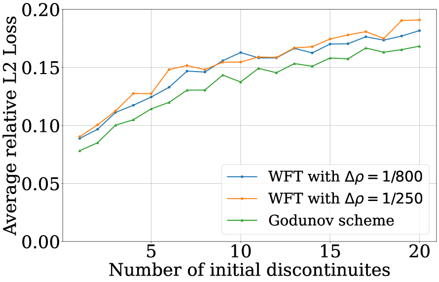
(a) The evolution of relative $L_{2}$ loss w.r.t. initial discontinuities

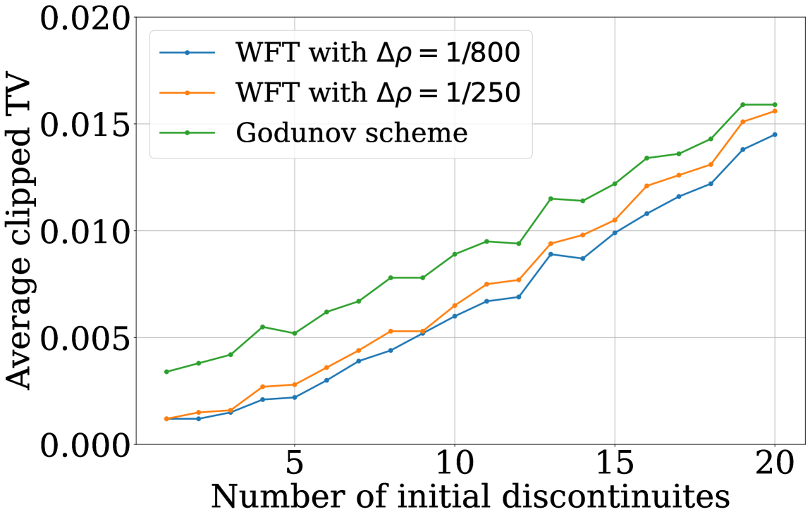
(b) The evolution of clipped TV w.r.t. initial discontinuities

Figure 10: Relative $L_{2}$ loss and diffusion error for complex data generated by WFT and Godunov scheme, trained up to 10 discontinuities and tested upto 20 discontinuities in initial condition on FNO

3.3.2 Problem II

This setup imposes time-invariant zero-flux boundary conditions, i.e., no mass enters or leaves the domain. This is achieved by assigning a very high value to the potential function as shown in equation (26), at the domain boundaries, thereby effectively preventing agents from moving towards the exits. This provides insight into the operator’s ability to handle an accumulating domain. Training data is generated using the Godunov scheme for a scenario up to three discontinuities in the initial density profile. Consequently, the primary challenge for the operator is to capture and adapt to the effect of a fully closed boundary across time, rather than learning multiple boundary states or abrupt transitions. As a result, this scenario is expected to be relatively straightforward for the operator to learn, while still offering a meaningful test of its capability to handle non-trivial boundary conditions consistently. As this problem is still an initial value problem with closed boundary, the operator training data is structured as shown in Figure 5, with different initial conditions.

Figure 11 presents the results for the scenario in which both exits are closed. In this configuration, the boundary conditions are relatively straightforward, resulting in minimal boundary influence on the interior of the domain. Consequently, the learning performance is significantly high.

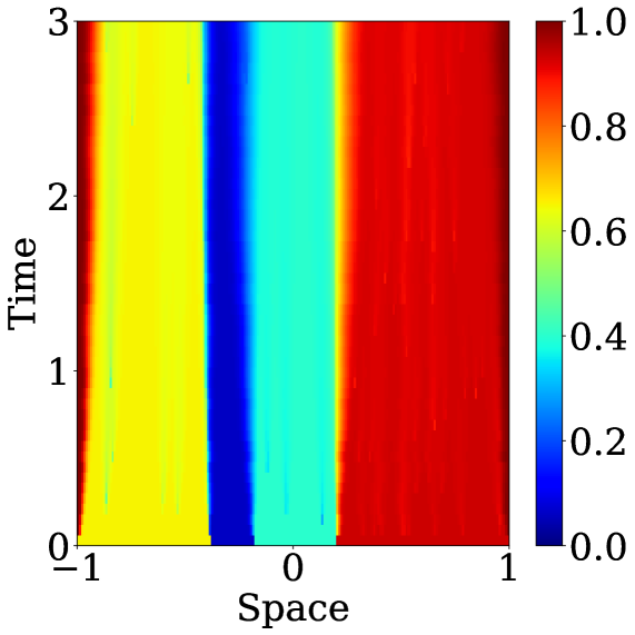
(a) Real Data

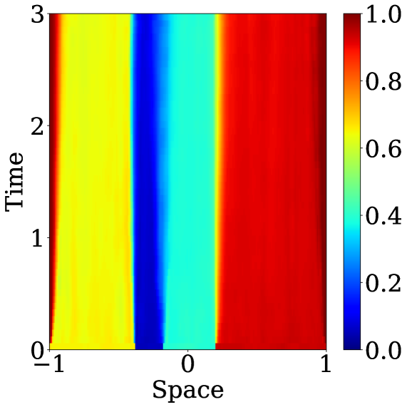
(b) Predicted Data

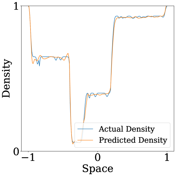
(c) Predicted Density at $t=0.5$

Figure 11: Prediction results with three discontinuities in initial condition and boundary conditions given by equation 26 (Train Loss: 0.032, Val Loss: 0.042, Test Loss: 0.042)

3.3.3 Problem III

To isolate and analyze the impact of boundary conditions on the learning behavior of neural operators, smooth, easy-to-learn initial conditions are used. Specifically, a zero discontinuity initial condition is constructed using a single Gaussian pulse with no discontinuities (see Subsection 2.3 for details). This ensures that the learning complexity is dominated by the boundary behavior rather than the initial condition itself. For this experiment, the dataset is generated using the Godunov scheme.

Given $\rho(t=0,x)$, two distinct boundary scenarios are considered:

• Absorbing boundary condition on both exits: Boundary condition given by equation (25) were adopted. This allows density to flow freely out of the domain which helps in modeling the movement of pedestrians that exit the corridor.

• Time varying absorbing boundary condition at left exit: To simulate realistic and time-varying boundary control, boundary conditions were adopted as given by equation (27).

These boundary conditions introduce time varying dynamics, enabling the evaluation of the neural operator’s sensitivity to temporal variations in boundary condition. Using a smooth initial condition (e.g. a Gaussian profile with no discontinuities), the complexity of the learning task is primarily driven by the boundary dynamics rather than the initial condition itself. For training purposes, each sample is structured as illustrated in Figure 6.

Table 4 shows the results for the case with Gaussian initial condition, where two cases were considered. Figure 12 shows the prediction results for the case when both exits are open. Figure 13, shows the results for the case where the left exit is closed non-periodically. For this case, a longer time interval is used to ensure that the density inside the domain goes to zero before simulation ends. This is because, if density remains non-zero inside the domain, any turning behavior exhibited will not be captured by the boundary condition unless it actually reaches the boundary. For time varying absorbing boundary condition, two configurations were used as input to train the operators:

• Initial Value Problem (IVP): using only the initial density profile as training input.

• Mixed Initial-Boundary Value Problem (MI-BVP): Combining the initial density profile with the boundary conditions as training input.

The results for these experiments are presented in Table 4 (columns 4 and 5, respectively). Here we see that the boundary conditions challenge the kernel-based representation of the neural operator by violating its core assumptions. The solution operator is no longer a simple translation-invariant convolution on the domain; it includes boundary integral terms and position dependent effects. A neural operator ignorant of this will tend to produce poor approximations, especially in scenarios where the solution is dominated by boundary driven effects. When boundary effects dominate, the shortcomings of the Green’s function assumption become more pronounced. The presence of boundaries means the true solution operator often decomposes into multiple components rather than a single integral kernel. Neural operators often approximate PDE solutions via a single kernel integral where the kernel acts like a Green’s function learned from data. In problems with nearly fixed or smoothly varying boundary conditions, a single integral kernel can capture the solution’s global behavior. However, when boundary conditions switch abruptly (e.g., an exit that randomly opens or closes), the actual PDE solution exhibits distinct regimes that a single static kernel struggles to learn. Relying on a single integral kernel forces the model to “average” conflicting boundary dynamics, often resulting in poor generalization as can be seen in Figure 13. As further illustrated in Figure 14, the NO approximation treats discontinuities inconsistently, dampening some jumps, exaggerating others, and occasionally missing them altogether, reinforcing the earlier assertion of its difficulty in capturing sharp features accurately.

Table 4: Relative $L_{2}$ loss for Data with Gaussian Initial Condition

Data	Num_sample	Both exit open	Left exit closed non-periodically (IVP)	Left exit closed non-periodically (MI-BVP)
Train	1000	0.042	0.167	0.042
Val	300	0.060	0.232	0.155
Test	300	0.053	0.220	0.155
Time per Epoch (s)		1.90	1.96	1.96

(a) Real Data

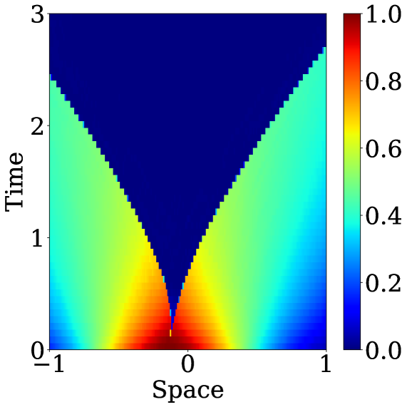
(b) Predicted Data

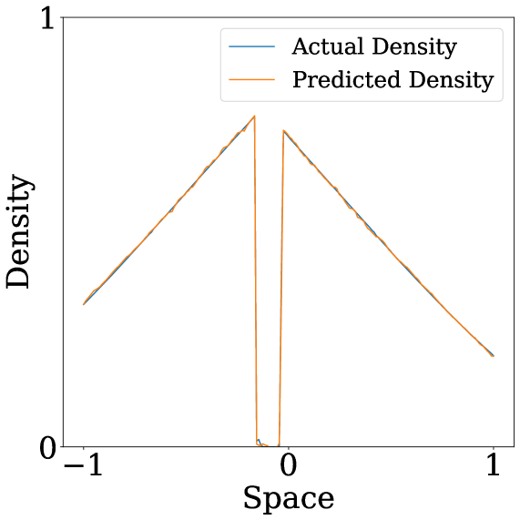
(c) Predicted Density at $t=0.5$

Figure 12: Prediction results with Gaussian initial condition

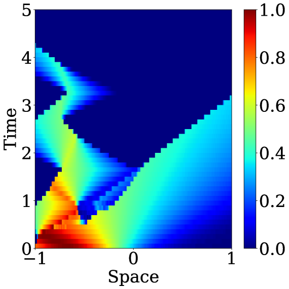
(a) Real Data

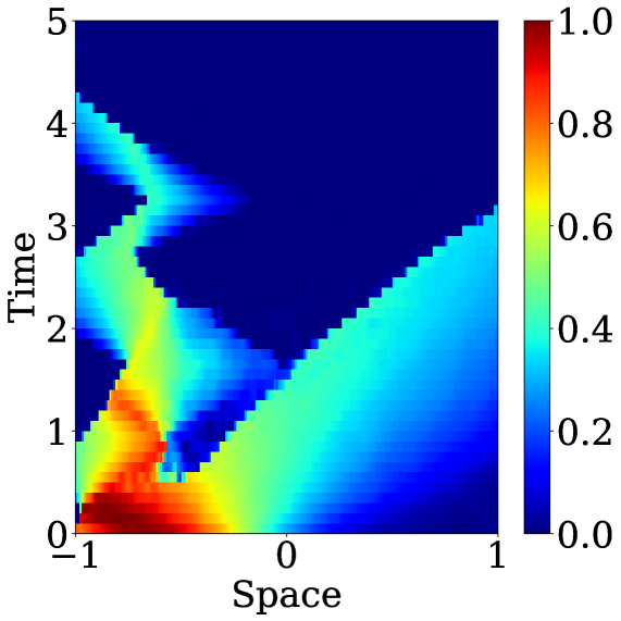
(b) Predicted Data

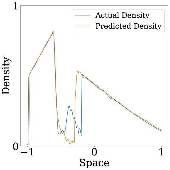
(c) Predicted Density at $t=0.9$

Figure 13: Prediction results under Gaussian initial conditions and boundary conditions given by equation 27.

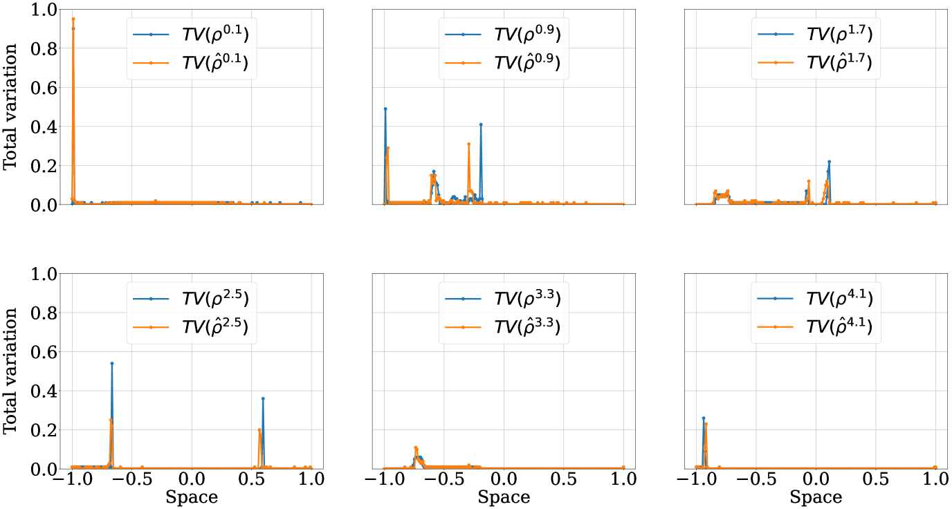
Figure 14: Total variation for the example sample shown in Figure 13 at different time steps trained on FNO

3.4 Numerical time-complexity

In this section, we compare the computational complexity of various methods used to solve the Hughes model across different discretizations. From the NO class, the FNO method is analyzed as it provides the fastest computations while maintaining a favorable trade-off with accuracy. A forward pass is performed on the entire test set (2400 samples), and the average computation time per sample is calculated. For both the Godunov scheme and the WFT algorithm, 150 samples are generated, and the average time per sample is calculated. The results are as shown in Table 5. Although the FNO outperforms traditional numerical schemes in terms of computational efficiency, its accuracy remains insufficient for reliably generating solutions to complex PDEs (Hughes model in this case). This gap motivates further exploration of neural operators that can achieve both high accuracy and efficiency.

Method	Parameters	Average time to solve given initial condition (ms)
FNO	$\Delta x=1/200$, $\Delta t=1/50$	Batch size = 1: $\mathbf{6}$ Batch size = 100: $\mathbf{0.4}$
Godunov	$\Delta x=1/100$, $\Delta t=1/100$	74
	$\Delta x=1/400$, $\Delta t=1/400$	2161
	$\Delta x^{*}=1/500$, $\Delta t^{*}=1/600$	4740
WFT Algorithm	$\Delta\rho=1/100$	95
	$\Delta\rho^{*}=1/250$	730
	$\mbox{}\quad\Delta\rho*=1/800$	2267

Table 5: Comparison of average time per sample and numerical parameters for different methods.
* Data at this discretization has been used for training.

4 Conclusion

In summary, our results reveal key limitations of current state-of-the-art neural operator when applied to complex nonlinear hyperbolic PDEs, such as the Hughes model for crowd dynamics. Although the tested neural operators perform reasonably well under simple conditions, their accuracy degrades noticeably as the complexity of initial and boundary conditions increases. This decline highlights a fundamental issue: existing architectures are not well-equipped to approximate solutions that contain multiple discontinuities, turning points, or nonlocal interactions, all of which are characteristic of the Hughes model. Moreover, we observe that the neural operators frequently fail to capture the precise location and strength of shock-like discontinuities; in many cases they either under-predict the sharpness or, conversely, artificially amplify or smooth out these abrupt transitions, leading to qualitatively incorrect flow patterns.

This study points to the need for new neural operator models or training strategies that are better suited to handling the challenges posed by nonlinear inviscid hyperbolic systems. Future research should focus on frameworks capable of handling abrupt transitions, thereby enhancing the robustness and reliability of predictive models in real-world applications.

5 Acknowledgment

This work was supported in part by the NYUAD Center for Interacting Urban Networks (CITIES), funded by Tamkeen under the NYUAD Research Institute Award CG001, and in part by the NYUAD Research Center on Stability, Instability, and Turbulence (SITE), funded by Tamkeen under the NYUAD Research Institute Award CG002. The views expressed in this article are those of the authors and do not reflect the opinions of CITIES, SITE, or their funding agencies.

6 Appendix

6.1 Hyperparameters

The hyperparameters for all the neural operators are provided in Table 6.

Table 6: Hyperparameters for FNO, MWT, and WNO models.

Hyperparameter	FNO	MWT	WNO
Batch size	40	40	40
Learning rate	0.01	0.01	0.01
Epochs	500	500	500
Step size	100	100	100
Weight decay rate	0.5	0.5	0.5
Fourier modes along t (modes_t)	10	–	–
Fourier modes along x (modes_x)	40	–	–
Projection dimension	80	–	80
Sample shape (t,x) WFT	50$\times$201	128$\times$128	49$\times$199
Sample shape (t,x) Godunov	50$\times$200	128$\times$128	49$\times$199
Weight decay	1e-3	1e-3	1e-3
Grid range (t,x)	[0:3,0:2]	[0:3,0:2]	[0:3,0:2]

Figure 15: Relative $L_{2}$ loss for complex data generated by Godunov scheme and trained up to ten discontinuities in initial condition on FNO with various Fourier modes

6.2 Algorithm: Godunov scheme for Hughes model

Algorithm 1 Data generation using Godunov scheme

1:Input: Grid $x=(x_{1},x_{2},\dots,x_{n})$, Initial density $\rho(t=0,x)$, Time step $\Delta t$, Spatial step $\Delta x$, Final time $T$

2:Output: Density $\rho(x,t)$

3:Initialize: $t\leftarrow 1$

4:while $t<T$ do

5:  Compute turning point using cost integral balance,

6:  for each grid index $x_{i}$ do

7:   $C_{\text{left}}(x_{i})\leftarrow\Delta x\sum_{j=x_{1}}^{x_{i}}\frac{1}{1-\rho(t-1,x_{j})}+\phi_{bc1}(t)$  $C_{\text{right}}(x_{i})\leftarrow\Delta x\sum_{j=x_{i}}^{x_{n}}\frac{1}{1-\rho(t-1,x_{j})}+\phi_{bc2}(t)$

8:  end for

9:  Find index $x_{i^{*}}$ that minimizes $|C_{\text{left}}(x_{i})-C_{\text{right}}(x_{i})|,\text{ note },\phi_{bc1}(t)=\phi_{bc2}(t)=0$

10:  Set turning point: $\xi(t)\leftarrow x_{i^{*}}$

11:  Define subdomains: left and right of $\xi(t)$

12:  With equal probability, choose one of the following:

13:$\Omega_{L}=\{x\leq\xi(t)\}$ and $\Omega_{R}=\{x>\xi(t)\}$ or $\Omega_{L}=\{x<\xi(t)\}$ and $\Omega_{R}=\{x\geq\xi(t)\}$

14:  Update right region $\Omega_{R}$ using Godunov scheme

15:  for each cell $x_{i}$ in $\Omega_{R}$ with $i=i^{*},i^{*}+1,\dots,n$ do

16:   Compute numerical flux $q_{i+1/2}=F(\rho(t-1,x_{i}),\rho(t-1,x_{i+1}))$

17:   Update:

$$\rho(t,x_{i})\leftarrow\rho(t-1,x_{i})-\frac{\Delta t}{\Delta x}\Bigl{(}q_{i+1/2}-q_{i-1/2}\Bigr{)}$$

18:  end for

19:  Update left region $\Omega_{L}$ using Godunov scheme

20:  for each cell $x_{i}$ in $\Omega_{L}$ with $i=i^{*},i^{*}-1,\dots,1$ do

21:   Compute numerical flux $q_{i-1/2}=F(\rho(t-1,x_{i}),\rho(t-1,x_{i-1}))$

22:   Update:

$$\rho(t,x_{i})\leftarrow\rho(t-1,x_{i})-\frac{\Delta t}{\Delta x}\Bigl{(}q_{i-1/2}-q_{i+1/2}\Bigr{)}$$

23:  end for

24:  $t\leftarrow t+\Delta t$

25:end while

26:Return $\rho(x,t)$

References

- [1] Carlos F Daganzo. Requiem for second-order fluid approximations of traffic flow. Transportation Research Part B: Methodological, 29(4):277–286, 1995.
- [2] Maziar Raissi, Paris Perdikaris, and George Em Karniadakis. Physics-informed neural networks: A deep learning framework for solving forward and inverse problems involving nonlinear partial differential equations. Journal of Computational Physics, 378:686–707, 2019.
- [3] Lu Lu, Pengzhan Jin, and George Em Karniadakis. Learning nonlinear operators via deeponet based on the universal approximation theorem of operators. Nature Machine Intelligence, 3(3):218–229, 2021.
- [4] Randall J LeVeque. Finite Volume Methods for Hyperbolic Problems, volume 31. Cambridge University Press, 2002.
- [5] Nikola Kovachki, Zongyi Li, Burigede Liu, Kamyar Azizzadenesheli, Kaushik Bhattacharya, Andrew Stuart, and Anima Anandkumar. Neural operator: Learning maps between function spaces with applications to pdes. Journal of Machine Learning Research, 24:1–97, 2023.
- [6] Zongyi Li, Nikola Kovachki, Kamyar Azizzadenesheli, Burigede Liu, Kaushik Bhattacharya, Andrew Stuart, and Anima Anandkumar. Fourier neural operator for parametric partial differential equations. ICLR, 2021.
- [7] Bilal Thonnam Thodi, Sai Venkata Ramana Ambadipudi, and Saif Eddin Jabari. Learning-based solutions to nonlinear hyperbolic pdes: Empirical insights on generalization errors. In Fifth Workshop on Machine Learning and the Physical Sciences (NeurIPS 2022), 2022.
- [8] Bilal Thonnam Thodi, Sai Venkata Ramana Ambadipudi, and Saif Eddin Jabari. Fourier neural operator for learning solutions to macroscopic traffic flow models: Application to the forward and inverse problems. Transportation Research Part C: Emerging Technologies, 160:104500, 2024.
- [9] Victor Morand, Nils Müller, Ryan Weightman, Benedetto Piccoli, Alexander Keimer, and Alexandre M Bayen. Deep learning of first-order nonlinear hyperbolic conservation law solvers. Journal of Computational Physics, 511:113114, 2024.
- [10] Qi Gao and Xuan Di. Comparative studies of neural operators for traffic state estimation. In 2024 IEEE 27th International Conference on Intelligent Transportation Systems (ITSC), pages 1992–1997. IEEE, 2024.
- [11] Archie J Huang and Shaurya Agarwal. Physics informed deep learning for traffic state estimation. In 2020 IEEE 23rd International Conference on Intelligent Transportation Systems (ITSC), pages 1–6. IEEE, 2020.
- [12] Roger L Hughes. A continuum theory for the flow of pedestrians. Transportation Research Part B: Methodological, 36(6):507–535, 2002.
- [13] Debora Amadori, Boris Andreianov, Marco Di Francesco, Simone Fagioli, Théo Girard, Paola Goatin, Peter Markowich, Jan F Pietschmann, Massimiliano D Rosini, Giovanni Russo, et al. The mathematical theory of hughes’ model: a survey of results. Crowd Dynamics, Volume 4: Analytics and Human Factors in Crowd Modeling, 2023.
- [14] Mohamed Ghattassi and Nader Masmoudi. Non-separable mean field games for pedestrian flow: Generalized hughes model. appear Math. Models Methods Appl. Sci., 2025.
- [15] Mohamed Ghattassi, Nader Masmoudi, and Eliot Pacherie. Stability analysis of the non-separable mean-fields games for pedestrian flow in large corridors. arXiv:2310.04702, appear SIAM J. Math. Anal., 2025.
- [16] Marco Di Francesco, Peter A Markowich, Jan-Frederik Pietschmann, and Marie-Therese Wolfram. On the hughes’ model for pedestrian flow: The one-dimensional case. Journal of Differential Equations, 250(3):1334–1362, 2011.
- [17] Rinaldo M Colombo, Paola Goatin, and Massimiliano D Rosini. On the modelling and management of traffic. ESAIM: Mathematical Modelling and Numerical Analysis, 45(5):853–872, 2011.
- [18] Paola Goatin and Matthias Mimault. The wave-front tracking algorithm for hughes’ model of pedestrian motion. SIAM Journal on Scientific Computing, 35(3):B606–B622, 2013.
- [19] Zongyi Li, Nikola Kovachki, Kamyar Azizzadenesheli, Burigede Liu, Kaushik Bhattacharya, Andrew Stuart, and Anima Anandkumar. Neural operator: Graph kernel network for partial differential equations. In Proceedings of the International Conference on Learning Representations (ICLR), 2020.
- [20] Zongyi Li, Nikola Kovachki, Kamyar Azizzadenesheli, Burigede Liu, Kaushik Bhattacharya, Andrew Stuart, and Anima Anandkumar. Multipole graph neural operator for parametric partial differential equations. arXiv preprint arXiv:2009.01938, 2020.
- [21] Gaurav Gupta, Xiongye Xiao, and Paul Bogdan. Multiwavelet-based operator learning for differential equations. Advances in Neural Information Processing Systems (NeurIPS), 34, 2021.
- [22] Tapas Tripura and Souvik Chakraborty. Wavelet neural operator: A neural operator for parametric partial differential equations. Computer Methods in Applied Mechanics and Engineering, 404:115783, 2023.
- [23] Jin Young Shin, Jae Yong Lee, and Hyung Ju Hwang. Pseudo-differential neural operator: Generalize fourier neural operator for learning solution operators of partial differential equations. Transactions on Machine Learning Research, 2024.
- [24] Wei Xiong, Xiaomeng Huang, Ziyang Zhang, Ruixuan Deng, Pei Sun, and Yang Tian. Koopman neural operator as a mesh-free solver of non-linear partial differential equations. Journal of Computational Physics, 513:113194, 2024.
- [25] Jose Antonio Carrillo, Stephan Martin, and Marie-Therese Wolfram. Numerical simulation of hughes’ model for pedestrian flow. ESAIM: Mathematical Modelling and Numerical Analysis, 50(2):575–600, 2016.
- [26] Ling Huang, Sze Chun Wong, Mengping Zhang, Chi-Wang Shu, and William HK Lam. Revisiting hughes‚Äô dynamic continuum model for pedestrian flow and the development of an efficient solution algorithm. Transportation Research Part B: Methodological, 43(1):127–141, 2009.
- [27] Zepeng Liu, SC Wong, Liangze Yang, Chi-Wang Shu, and Mengping Zhang. Multi-element probabilistic collocation solution for dynamic continuum pedestrian models with random inputs. Transportation Research Part C: Emerging Technologies, 174:105104, 2025.
- [28] Sergei K Godunov and Ihor Bohachevsky. Finite difference method for numerical computation of discontinuous solutions of the equations of fluid dynamics. Matematičeskij sbornik, 47(3):271–306, 1959.
- [29] Hongkai Zhao. A fast sweeping method for eikonal equations. Mathematics of computation, 74(250):603–627, 2005.