Efficient Matching of Some Fundamental
Regular Expressions with Backreferences

Abstract

Regular expression matching is of practical importance due to its widespread use in real-world applications. In practical use, regular expressions are often used with real-world extensions. Accordingly, the matching problem of regular expressions with real-world extensions has been actively studied in recent years, yielding steady progress. However, backreference, a popular extension supported by most modern programming languages such as Java, Python, JavaScript and others in their standard libraries for string processing, is an exception to this positive trend. In fact, it is known that the matching problem of regular expressions with backreferences (rewbs) is theoretically hard and the existence of an asymptotically fast matching algorithm for arbitrary rewbs seems unlikely. Even among currently known partial solutions, the balance between efficiency and generality remains unsatisfactory. To bridge this gap, we present an efficient matching algorithm for rewbs of the form $e_{0}(e)_{1}e_{1}\backslash 1e_{2}$ where $e_{0},e,e_{1},e_{2}$ are pure regular expressions, which are fundamental and frequently used in practical applications. It runs in quadratic time with respect to the input string length, substantially improving the best-known cubic time complexity for these rewbs. Our algorithm combines ideas from both stringology and automata theory in a novel way. We leverage two techniques from automata theory, injection and summarization, to simultaneously examine matches whose backreferenced substrings are either a fixed right-maximal repeat or its extendable prefixes, which are concepts from stringology. By further utilizing a subtle property of extendable prefixes, our algorithm correctly decides the matching problem while achieving the quadratic-time complexity.

1 Introduction

A regular expression is a convenient way to specify a language (i.e., a set of strings) using concatenation ($\cdot$), disjunction ($\mid$) and iteration ($\ast$). The regular expression matching problem (also known as regular expression membership testing) asks whether a given string belongs to the language of a given regular expression. This problem is of practical importance due to its widespread use in real-world applications, particularly in format validation and pattern searching. In 1968, Thompson presented a solution to this problem that runs in $O({nm})$ time where $n$ denotes the length of the input string and $m$ the length of the input regular expression [44]. We refer to his method, which constructs a nondeterministic finite automaton (NFA) and simulates it, as NFA simulation.

The matching problem of real-world regular expressions becomes increasingly complex due to its practical extensions such as lookarounds and backreferences. Unfortunately, reducing the matching of real-world regular expressions to that of pure ones is either inefficient or impossible. In fact, although adding positive lookaheads (a type of lookaround) does not increase the expressive power of regular expressions [32, 7], the corresponding NFAs can inevitably become enormous [31]. Worse still, adding backreferences makes regular expressions strictly more expressive, meaning that an equivalent NFA may not even exist.

Nevertheless, most modern programming languages, such as Java, Python, JavaScript and more, support lookarounds and backreferences in their standard libraries for string processing. The most widely used implementation for the real-world regular expression matching is backtracking [42], an algorithm that is easy to implement and extend. On the other hand, the backtracking implementation suffers from a major drawback in that it takes exponential time in the worst case with respect to the input string length. This exponential-time behavior poses the risk of ReDoS (regular expression denial of service), a type of DoS attack that exploits heavy regular expression matching to cause service downtime, making it a critical security issue (refer to Davis et al. [14] for details on its history and case studies). In response, RE2, a regular expression engine developed by Google, has deferred supporting lookarounds and backreferences, thereby ensuring $O({nm})$ time complexity using NFA simulation.

Regarding lookarounds, several recent papers have proposed groundbreaking $O({nm})$-time solutions to the matching problem of regular expressions with lookarounds [30, 21, 6], yet regarding backreferences, the outlook is bleak. The matching problem of regular expressions with backreferences (rewbs for short) is well known for its theoretical difficulties. Aho showed that the rewb matching problem is NP-complete [3]. Moreover, rewbs can be considered a generalization of Angluin’s pattern languages (also known as patterns with variables) [4]; even when restricted to this, its matching problem is NP-complete with respect to the lengths of both a given string and a given pattern [4, 16, 39], and its NP-hardness [18] as well as W[1]-hardness [19] are known for certain fixed parameter settings. The best-known matching algorithm for rewbs with at most $k$ capturing groups runs in $O({n^{2k+2}m})$ time [40, 38] (With a slight modification, the time complexity can be reduced in $O({n^{2k+1}m})$ time; see Section˜4).

Therefore, the existence of an efficient worst-case time complexity algorithm that works for any rewb seems unlikely, necessitating researchers to explore efficient algorithms that work for some subset of rewbs [37, 38, 20]. Nevertheless, all existing solutions either have high worst-case time complexity or impose non-trivial constraints on the input rewbs, and finding a good balance between efficiency and generality remains an open issue.

To bridge this gap, we present an efficient matching algorithm for rewbs of the form $e_{0}(e)_{1}e_{1}\backslash 1e_{2}$, where $e_{0},e,e_{1},e_{2}$ are pure regular expressions, which are fundamental and frequently encountered in practical applications. While the best-known algorithm for these rewbs is the one stated above and it takes $O({n^{4}m})$ (or $O({n^{3}m})$) time because $k=1$ for these rewbs, our algorithm runs in $O(n^{2}m^{2})$ time, improving the best-known time complexity for these rewbs with respect to the input string length $n$ from cubic to quadratic. The key appeal of this improvement lies in the replacement of the input string length $n$ with the expression length $m$. Because $n$ is typically much larger than $m$, this improvement is considerable.

These rewbs are of both practical and theoretical interest. From a practical perspective, these rewbs account for a large proportion of the actual usage of backreferences. In fact, we have confirmed that, among the dataset collected in a large-scale empirical study conducted by Davis et al. [14], which consists of real-world regular expressions used in npm and PyPI projects, approximately 57% of the non-pure rewbs (1,659/2,909) are of this form.

Additionally, the matching problem of rewbs of this form is a natural generalization of a well-studied foundational problem, making it theoretically interesting. A square (also known as tandem repeat) is a string $\alpha\alpha$ formed by juxtaposing the same string $\alpha$. The problem of deciding whether a given string contains a square is of interest in stringology, and has been well studied [29, 12]. The rewb matching considered in this paper can be viewed as a generalization of the problem by regular expressions.

We now provide an overview of our new algorithm. A novel aspect of the algorithm is that, unlike previous algorithms for rewb matching or square finding, it combines ideas from both stringology and automata theory. Our algorithm utilizes the suffix array of the input string to efficiently enumerate candidates for backreferenced substrings (i.e., the contents of $\backslash 1$). Once a candidate $\alpha$ is fixed, the matches whose backreferenced substring is $\alpha$ can be examined in $O({nm})$ time in almost the same way as NFA simulation. Because the number of candidate substrings is $\Theta({n^{2}})$, this gives an $O({n^{3}m})$-time algorithm (see Remark˜3.8 for details). Next, we improve this baseline algorithm by extending the NFA simulation to simultaneously examine all matches whose backreferenced substrings are either a right-maximal repeat or its extendable prefixes, instead of examining each candidate individually. Because the new NFA simulation requires $O({m^{2}})$ time at each step and the number of right-maximal repeats is at most $n-1$, our algorithm runs in $O({n^{2}m^{2}})$ time.

A key challenge is how to do all the examinations within time linear in $n$ for each fixed right-maximal repeat $\alpha$. To address this, we incorporate two techniques from automata theory, injection and summarization. Each of these techniques is fairly standard on its own (see Section˜4 for their applications in prior work), but the idea of combining them is, to our knowledge, novel. Additionally, we leverage a subtle property of $\alpha$-extendable prefixes to do the examinations correctly within time linear in $n$ even when occurrences of $\alpha$ may overlap (see Section˜3.2).

The rest of the paper is organized as follows. Section˜2 defines the key concepts in this paper, namely NFA simulation and right-maximal repeats. Section˜3 presents our algorithm, which is the main contribution of this paper. Section˜4 discusses related work and Section˜5 presents the conclusion and future work. Omitted proofs are in the appendix.

2 Preliminaries

Let $\Sigma$ be a set called an alphabet, whose elements are called characters. A string $w$ is a finite sequence $a_{1}\cdots a_{n}$ of characters $a_{1},\dots,a_{n}$, and we write $|w|$ for the number $n$ of characters in the sequence. The empty string is written as $\varepsilon$. For integers $i,j\geq 0$, we write $[i,j]$ for the set of integers between $i$ and $j$. For $i,j\in[1,n]$, we write $w[i..j]$ for the substring $a_{i}\cdots a_{j}$. In particular, $w[i]:=w[i..i]=a_{i}$ is called the character at position $i$, $w[..i]:=w[1..i]$ is called the prefix up to position $i$ and $w[i..]:=w[i..n]$ is called the suffix from position $i$. We regard $w[i+1..i]$ as $\varepsilon$. A regular expression $e$ and its language denoted by $L(e)$ are defined in the standard way.

First, we define the matching problem for rewbs of the form mentioned earlier. Note that in full, rewbs are capable of more versatile expressions, such as using reference more than once (e.g., $(a^{\ast})_{1}\backslash 1\backslash 1$) or using multiple capturing groups (e.g., $(a^{\ast})_{1}(b^{\ast})_{2}\backslash 1\backslash 2$)). For the full syntax and semantics of rewbs, refer to [20].

Definition .

Given regular expressions $e_{0},e,e_{1},e_{2}$, the language of rewb $r=e_{0}(e)_{1}e_{1}\backslash 1e_{2}$, denoted by $L(r)$, is $\{w_{0}\alpha w_{1}\alpha w_{2}\mid w_{i}\in L(e_{i})(i=0,1,2),\alpha\in L(e)\}$.

A regular expression $e$ matches a string $w$ if $w\in L(e)$. The matching problem for regular expressions is defined to be the problem of deciding whether a given regular expression matches a given string, and similarly for rewbs.

Next, we review a classical solution of the regular expression matching.

Definition .

A nondeterministic finite automaton (NFA) $N$ is a tuple $(Q,\delta,q_{0},F)$ where $Q$ is a finite set of states, $\delta\colon Q\times(\Sigma\cup\{\varepsilon\})\to\operatorname{\mathcal{P}}(Q)$ is a transition relation, $q_{0}\in Q$ is an initial state, $F\subseteq Q$ is a set of accept states.

The transitive closure of a transition relation $\delta$ with the second argument fixed at $\varepsilon$ is called $\varepsilon$-closure operator and written as $\operatorname{cl_{\varepsilon}}$. Further, we lift $\operatorname{cl_{\varepsilon}}\colon Q\to\operatorname{\mathcal{P}}(Q)$ to $\operatorname{\mathcal{P}}(Q)\to\operatorname{\mathcal{P}}(Q)$ by taking unions, i.e., $\operatorname{cl_{\varepsilon}}{S}:=\bigcup_{q\in S}\operatorname{cl_{\varepsilon}}(q)$. For a state $q$ and a character $a$, $\Delta(q,a)$ is $\operatorname{cl_{\varepsilon}}{\delta(q,a)}$, which informally consists of states reachable by repeating $\varepsilon$-moves from states that are reachable from $q$ by $a$. As before, we extend $\Delta$ by setting $\Delta(S,a):=\bigcup_{q\in S}\Delta(q,a)$. Also, for a string $w$, we define $\Delta(S,w)$ as $\Delta(S,\varepsilon):=S$ and $\Delta(S,wa):=\Delta(\Delta(S,w),a)$. Thus, the language $L(N)$ of an NFA $N$ is the set of strings $w$ such that $\Delta(\operatorname{cl_{\varepsilon}}(q_{0}),w)\cap F\neq\emptyset$.

The NFA simulation of an NFA $N$ on a string $w$ of length $n$ is the following procedure for calculating $\Delta(\operatorname{cl_{\varepsilon}}(q_{0}),w)$ [44]. Let $q_{0}$ denote the initial state of $N$. First, $S^{(0)}:=\operatorname{cl_{\varepsilon}}(q_{0})$ is calculated, and then $S^{(i)}:=\Delta(S^{(i-1)},w[i])$, called the simulation set at position $i$, is sequentially computed from $S^{(i-1)}$ for each $i\in[1,n]$. Clearly, we have $w\in L(N)\iff S^{(n)}\cap F\neq\emptyset$.

This gives a solution to the regular expression matching in $O({nm})$ time and $O({m})$ space where $n$ is the length of the input string $w$ and $m$ that of the input regular expression $e$. First, convert $e$ to an equivalent NFA $N_{e}$ whose number of states and transitions are both $O({m})$ using the standard construction, then run the NFA simulation of $N_{e}$ on $w$. Finally, check whether the last simulation set $S^{(n)}$ contains any accept state of $N_{e}$. Each step of the NFA simulation can be done in $O({m})$ time using breadth-first search. Also, the procedure can be implemented in $O({m})$ space by reusing the same memory for each $S^{(i)}$.

Remark 2.1.

We call acceptance testing the disjointness testing of a simulation set $S$ and a set $F$ of accept states, as performed above. An acceptance test succeeds if $S\cap F\neq\emptyset$.

Acceptance testing of an intermediate simulation set is also meaningful. We can check whether $e$ matches each prefix $w[..i]$ with the same asymptotic complexity by testing at each position $i$. The same can be done for the suffixes by reversing $e$ and $w$.

Next, we review right-maximal repeats and extendable prefixes. Let $w$ be a string. A nonempty string $\alpha$ occurs at position $i$ in $w$ if $w[i..i+|\alpha|-1]=\alpha$. Two distinct occurrences of $\alpha$ at positions $i<j$ overlap if $j<i+|\alpha|$. A repeat of $w$ is a nonempty string that occurs in $w$ more than once. A repeat $\alpha$ is called right-maximal if $\alpha$ occurs at two distinct positions $i,j$ such that the right-adjacent characters are different (i.e., $w[i+|\alpha|]\neq w[j+|\alpha|]$). For example, the right-maximal repeats of mississimiss are i, iss, issi, miss, s, si, ss and ssi. In general, the number of repeats of a string of length $n$ is $\Theta({n^{2}})$, while that of right-maximal repeats is at most $n-1$ [23].

For any non-right-maximal repeat $\alpha$, all the right-adjacent positions of the occurrences of $\alpha$ have the same character. By repeatedly extending $\alpha$ with this, we will eventually obtain the right-maximal repeat, denoted by $\overrightarrow{\alpha}$. We define $\overrightarrow{\alpha}:=\alpha$ for a right-maximal repeat $\alpha$. A prefix $\beta$ of $\alpha$ such that $\overrightarrow{\beta}=\alpha$ is called $\alpha$-extendable prefix of $\alpha$. Two occurrences of an $\alpha$-extendable prefix $\beta$ are $\alpha$-separable in $w$ if the $\alpha$’s extended from the $\beta$’s have no overlap.

Finally, we mention the enumeration subroutine used in our algorithm. Abouelhoda et al. presented an $O({n})$-time enumeration algorithm for right-maximal repeats [2]. By slightly modifying this, we obtain an $O({n^{2}})$-time algorithm EnumRM that enumerates each right-maximal repeat $\alpha$ with the sorted array $\mathsf{Idx}_{\alpha}$ of all starting positions of the occurrences of $\alpha$. We call $\mathsf{Idx}_{\alpha}$ the occurrence array of $\alpha$ in $w$. For details, see Appendix˜A.

3 Efficient Matching

In this section, we show an efficient matching algorithm for rewbs of the form $e_{0}(e)_{1}e_{1}\backslash 1e_{2}$, which is the main contribution of this paper.

Theorem 3.1.

The matching problem for rewbs of the form $e_{0}(e)_{1}e_{1}\backslash 1e_{2}$ where $e_{0},e,e_{1},e_{2}$ are regular expressions can be solved in $O({n^{2}m^{2}})$ time and $O({n+m^{2}})$ space. Here, $n$ denotes the length of the input string and $m$ that of the input rewb. More precisely, let $m_{e_{0}}{},m_{e}{},m_{e_{1}}{},m_{e_{2}}{}$ denote the length of $e_{0},e,e_{1},e_{2}$ respectively, and $\mu_{\mathrm{right}}$ the number of right-maximal repeats of the input string, which is at most $n-1$. Then, the problem can be solved in $O({n^{2}+n(m_{e_{0}}{}+m_{e_{2}}{})+\mu_{\mathrm{right}}n(m_{e}{}+m_{e_{1}}^{2})})$ time and $O({n+\max\{m_{e_{0}}{},m_{e}{},m_{e_{2}}{},m_{e_{1}}^{2}\}})$ space.

Let $r$ be a rewb $e_{0}(e)_{1}e_{1}\backslash 1e_{2}$ and $w$ be a string. The overview of our matching algorithm for $r$ and $w$ is as follows. We assume without loss of generality that $e$ does not match $\varepsilon$. We show an $O({n(m_{e}{}+m_{e_{1}}^{2})})$-time and $O({n+m_{e}{}+m_{e_{1}}^{2}})$-space subprocedure $\textnormal{{Match}}(\alpha,\mathsf{Idx}_{\alpha})$ ($\textnormal{{Match}}(\alpha)$ for short) that takes a right-maximal repeat $\alpha$ and its occurrence array $\mathsf{Idx}_{\alpha}$, and simultaneously examines all matches whose backreferenced substrings (i.e., the contents of $\backslash 1$) are $\alpha$-extendable prefixes of $\alpha$. We state in advance the correctness Match is expected to satisfy:

Lemma 3.2 (Correctness of Match).

Let $\alpha$ be a right-maximal repeat of $w$. There exists a prefix $\beta$ of $\alpha$ such that $e$ matches $\beta$ and $e_{0}\beta e_{1}\beta e_{2}$ matches $w$ if $\textnormal{{Match}}(\alpha)$ returns $\mathbf{true}$. Conversely, $\textnormal{{Match}}(\alpha)$ returns $\mathbf{true}$ if there exists an $\alpha$-extendable prefix $\beta$ of $\alpha$ such that $e$ matches $\beta$ and $e_{0}\beta e_{1}\beta e_{2}$ matches $w$.

Remark 3.3.

Note that, interestingly, the correctness is incomplete on its own. That is, when there is a prefix $\beta$ of $\alpha$ such that a match with $\beta$ as the backreferenced substring exists, $\textnormal{{Match}}(\alpha)$ is guaranteed to return $\mathbf{true}$ if $\beta$ is $\alpha$-extendable, but it can return $\mathbf{false}$ if $\beta$ is not $\alpha$-extendable. Still, the correctness of the overall algorithm Main described below holds because it runs Match on every right-maximal repeat, and a match with a non-$\alpha$-extendable prefix $\beta$ is guaranteed to be reported by another execution of Match (namely, by $\textnormal{{Match}}(\overrightarrow{\beta})$). Formally, see the proof of Theorem˜3.1 described below.

Additionally, we precompute a Boolean array $\mathsf{Pre}$ (resp. $\mathsf{Suf}$) that stores which prefix (resp. suffix) of $w$ is matched by $e_{0}$ (resp. $e_{2}$). More precisely, we precompute arrays $\mathsf{Pre},\mathsf{Suf}$ such that $\mathsf{Pre}[i]=\mathbf{true}\iff w[..i]\in L(e_{0})$ for $i\in[0,n]$ and $\mathsf{Suf}[j]=\mathbf{true}\iff w[j..]\in L(e_{2})$ for $j\in[1,n+1]$. This can be done in $O({n(m_{e_{0}}{}+m_{e_{2}}{})})$ time and $O({n+\max\{m_{e_{0}}{},m_{e_{2}}{}\}})$ space as mentioned in Remark˜2.1. Also, we fix an NFA $N_{e_{1}}=(Q,\delta,q_{0},F)$ equivalent to the middle subexpression $e_{1}$.

The overall matching algorithm Main is constructed as follows. It first constructs $\mathsf{Pre},\mathsf{Suf}$ and $N_{e_{1}}$, and then runs the $O({n^{2}})$-time and $O({n})$-space enumeration algorithm EnumRM from the previous section. Each time EnumRM outputs $\alpha$ and $\mathsf{Idx}_{\alpha}$, it runs Match with them as input. Main returns $\mathbf{true}$ if $\textnormal{{Match}}(\alpha)$ returns $\mathbf{true}$ for some $\alpha$; otherwise, it returns $\mathbf{false}$.

Proof 3.4 (Proof of Theorem˜3.1.).

It suffices to show the correctness of Main, namely Main returns $\mathbf{true}$ if and only if $r$ matches $w$. If the input string $w$ has a match for $r$, the (nonempty) backreferenced substring is a repeat $\beta$ of $w$ that $e$ matches. Then, $\textnormal{{Match}}(\overrightarrow{\beta})$ returns $\mathbf{true}$ by Lemma˜3.2. The converse also follows from the lemma.

In what follows, we present the detailed behavior of the subroutine Match, incrementally progressing from simple cases to more complex ones.

3.1 The Case of Nonoverlapping Right-Maximal Repeats

Let $\alpha$ be a fixed right-maximal repeat of the input string $w$. In this subsection, for simplicity, we consistently assume that no occurrences of $\alpha$ overlap with each other. We call such an $\alpha$ nonoverlapping right-maximal repeat. We first introduce in Section˜3.1.1 a way to examine matches whose backreferenced substring is $\alpha$ itself, namely NFA simulation with auxiliary arrays and a technique called injection. Then, in Section˜3.1.2, we extend it to simultaneously examine all matches whose backreferenced substrings are $\alpha$-extendable prefixes of $\alpha$, instead of examining $\alpha$ individually. There, in addition to injection, we use a technique called summarization.

3.1.1 Only the right-maximal repeat itself

Let $r_{\alpha}$ denote the (pure) regular expression $e_{0}\alpha e_{1}\alpha e_{2}$. We give an $O({nm})$-time algorithm $\textnormal{{Match1}}(\alpha)$ that checks whether $r_{\alpha}$ matches $w$. It runs the NFA simulation of $N_{e_{1}}$ using the arrays $\mathsf{Pre}$, $\mathsf{Suf}$ and $\mathsf{Idx}_{\alpha}$ as oracles.

The injection technique is grounded on the following property.

Lemma 3.5.

For any sets of states $S,T$ and any strings $u,v$, $\Delta(S,uv)=\Delta(\Delta(S,u),v)$ and $\Delta(S,u)\cup\Delta(T,u)=\Delta(S\cup T,u)$.

The lemma implies the following equation:

$$\Delta(\operatorname{cl_{\varepsilon}}(q_{0}),uv)\cup\Delta(\operatorname{cl_{\varepsilon}}(q_{0}),v) =\Delta(\Delta(\operatorname{cl_{\varepsilon}}(q_{0}),u),v)\cup\Delta(\operatorname{cl_{\varepsilon}}(q_{0}),v)$$

$$=\Delta(\Delta(\operatorname{cl_{\varepsilon}}(q_{0}),u)\cup\operatorname{cl_{\varepsilon}}(q_{0}),v).$$

Therefore, we can simultaneously check whether $e$ matches either a string $uv$ or its suffix $v$ as follows: in the NFA simulation on $uv$, when $u$ has been processed, replace the current simulation set $\Delta(\operatorname{cl_{\varepsilon}}(q_{0}),u)$ with the union of it and $\operatorname{cl_{\varepsilon}}(q_{0})$, and then continue with the remaining simulation on $v$. We call this replacement injection. More generally, for any positions $i_{1}<i_{2}<\cdots<i_{l}\leq j$, we can check whether $e$ matches any of $w[i_{1}..j],\dots,w[i_{l}..j]$ by testing the injected simulation set immediately after the character $w[j]$, namely $\Delta(\cdots\Delta(\Delta(\operatorname{cl_{\varepsilon}}(q_{0}),w[i_{1}..i_{2}-1])\cup\operatorname{cl_{\varepsilon}}(q_{0}),w[i_{2}..i_{3}-1])\cup\operatorname{cl_{\varepsilon}}(q_{0})\cdots,w[i_{l}..j])$.

Correctness : See Lemma˜3.7.

1 $i_{prev}\leftarrow\bot;\;\;S\leftarrow\emptyset;\;\;i_{que}\leftarrow\bot;\;\;(\Delta,\operatorname{cl_{\varepsilon}}(q_{0}),F)\leftarrow N_{e_{1}}$

2 if $e$ does not match $\alpha$ then  return $\mathbf{false}$

3 for $i_{next}\in\mathsf{Idx}_{\alpha}$ do

4    if $i_{que}\neq\bot$ then

5       for $i\leftarrow i_{prev}$ to $i_{next}-1$ do

6          if $S\neq\emptyset$ then  $S\leftarrow\Delta(S,w[i])$

7          if $i=i_{que}$ then  $S\leftarrow S\cup\operatorname{cl_{\varepsilon}}(q_{0})$ /* Injection */

8         

9      if $S\cap F\neq\emptyset$ and $\mathsf{Suf}[i_{next}+|\alpha|]$ then  return $\mathbf{true}$

10      

11   $i_{prev}\leftarrow i_{next}$

12    if $\mathsf{Pre}[i_{prev}-1]$ then  $i_{que}\leftarrow i_{prev}+|\alpha|-1$

13   

return $\mathbf{false}$

Algorithm 1 $\textnormal{{Match1}}(\alpha)$

We now explain $\textnormal{{Match1}}(\alpha)$ whose pseudocode is shown in Algorithm˜1. First, it checks if $e$ matches $\alpha$ and returns $\mathbf{false}$ if it is false; otherwise, the algorithm continues running. Let $i_{1}<i_{2}<\cdots$ be the positions in $\mathsf{Idx}_{\alpha}$. Then, it searches for the starting position $i_{j_{1}}$ of the leftmost occurrence of $\alpha$ such that $e_{0}$ matches the prefix $w[..i_{j_{1}}-1]$ to the left of the $\alpha$ (lines 1, 1 and 1). Remark that the $\alpha$ at position $i_{j_{1}}$ is the leftmost candidate that the left $\alpha$ of $r_{\alpha}$ may correspond to in a match.

If $i_{j_{1}}$ is found, it starts an NFA simulation of $N_{e_{1}}$ from the position $i_{j_{1}}+|\alpha|$ immediately to the right of the $\alpha$ at position $i_{j_{1}}$ by setting $S$ to be $\operatorname{cl_{\varepsilon}}(q_{0})$ immediately after the character $w[i_{j_{1}}+|\alpha|-1]$ (line 1). Note that $S$ is $\emptyset$ prior to the assignment. In what follows, let $i_{j_{2}},i_{j_{3}},\dots$ denote the starting positions of the $\alpha$’s to the right of the $\alpha$ at position $i_{j_{1}}$ in sequence. Note that, unlike in the case of $i_{j_{1}}$, we do not assume that $e_{0}$ matches the prefix $w[..i_{j_{k-1}}]$ for $i_{j_{k}}$, i.e., $j_{k}=j_{1}+k-1$ ($k\geq 2$).

Next, the algorithm resumes the simulation and proceeds until the character $w[i_{j_{2}}-1]$ (lines 1 and 1). Then, it performs the acceptance testing $S\cap F\neq\emptyset$ (line 1). If it succeeds, $e_{0}\alpha e_{1}\alpha$ matches $w[..i_{j_{2}}+|\alpha|-1]$ by matching the two $\alpha$’s to $w[i_{j_{1}}..i_{j_{1}}+|\alpha|-1]$ and $w[i_{j_{2}}..i_{j_{2}}+|\alpha|-1]$. Accordingly, the algorithm further checks whether $e_{2}$ matches the remaining suffix $w[i_{j_{2}}+|\alpha|..]$ by looking at $\mathsf{Suf}[i_{j_{2}}+|\alpha|]$. If it is $\mathbf{true}$, $r_{\alpha}$ matches $w$ and the algorithm returns $\mathbf{true}$. Otherwise, there is no possibility that $r_{\alpha}$ matches $w$ in a way that the right $\alpha$ of $r_{\alpha}$ matches the $\alpha$ at position $i_{j_{2}}$, and the algorithm continues running.

In this way, the algorithm proceeds from position $i_{j_{k-1}}$ to position $i_{j_{k}}$ for $k=2,3,\dots$ as follows, while assigning $i_{j_{k-1}}$ and $i_{j_{k}}$ to variables $i_{prev}$ and $i_{next}$ respectively at each $k$: (i) it processes the substring $w[i_{prev}..i_{prev}+|\alpha|-1]$ (lines 1 and 1), and then (ii) injects $\operatorname{cl_{\varepsilon}}(q_{0})$ into the simulation set $S$ if the $\alpha$ at position $i_{prev}$ is a candidate that the left $\alpha$ of $r_{\alpha}$ may correspond to in a match (i.e., if $e_{0}$ matches $w[..i_{prev}-1]$) (line 1). Next, (iii) it resumes the simulation and proceeds until the character $w[i_{next}-1]$ (lines 1 and 1), and then (iv) performs the acceptance testing and checks whether $e_{2}$ matches the remaining suffix $w[i_{next}+|\alpha|..]$ (line 1). Finally, (v) it updates $i_{prev}$ using $i_{next}$ and if the $\alpha$ at $i_{j_{k}}$ is a candidate that the left $\alpha$ of $r_{\alpha}$ may correspond to in a match, then keep its right-adjacent position $i_{j_{k}}+|\alpha|-1$ in $i_{que}$ for future injection (lines 1 and 1). If step (iv) succeeds for some $j$, it returns $\mathbf{true}$; otherwise, it returns $\mathbf{false}$.

Clearly, Match1 runs in linear time with respect to $n$ because each character in $w$ is processed at most once. For the correctness of the algorithm, the following is essential.

Proposition 3.6.

Let $i_{1}<i_{2}<\cdots$ be the positions in $\mathsf{Idx}_{\alpha}$. Every time line 1 is reached at an iteration with $i_{next}=i_{j}$, $S=\bigcup_{j^{\prime}\in J^{\prime}}\Delta(\operatorname{cl_{\varepsilon}}(q_{0}),w[i_{j^{\prime}}+|\alpha|,i_{j}-1])$ where $J^{\prime}=\{j^{\prime}\in[1,|\mathsf{Idx}_{\alpha}|]\mid i_{j^{\prime}}+|\alpha|\leq i_{j}\text{ and }w[..i_{j^{\prime}}-1]\in L(e_{0})\}$.

Lemma 3.7 (Correctness of Match1).

Let $\alpha$ be a nonoverlapping right-maximal repeat of $w$. Then, $\textnormal{{Match1}}(\alpha)$ returns $\mathbf{true}$ if and only if $e$ matches $\alpha$ and $r_{\alpha}$ matches $w$.

Remark 3.8.

In fact, Match1 works correctly for any repeat $\alpha$ and not only right-maximal ones. This gives an $O(n^{3}m)$-time matching algorithm for rewbs of our form by modifying EnumRM to output not only all right-maximal repeats but all repeats. As mentioned in the introduction, we note that this time complexity itself can also be achieved by existing algorithms. Further improvements in time complexity require additional ideas that we describe in the following sections as extensions of the baseline algorithm Match1 that we just presented.

Remark 3.9.

An essential and interesting property of the algorithm is that if it returns $\mathbf{true}$, the existence of a match is guaranteed, but we do not know where $e$ matches. This is because injecting $\operatorname{cl_{\varepsilon}}(q_{0})$ into the simulation set in an NFA simulation means identifying the current position with the starting position of the NFA simulation.

3.1.2 The extendable prefixes of the right-maximal repeat

Recall that $\alpha$ is a fixed nonoverlapping right-maximal repeat of $w$. We extend Match1 to simultaneously examine all matches whose backreferenced substrings are $\alpha$-extendable prefixes of $\alpha$. Note that $\alpha$ itself is always $\alpha$-extendable. To this end, we split the NFA simulation of Match1 in two phases.

We first introduce a technique called summarization. Let $q_{1},\dots,q_{m_{1}{}}$ be the states of the NFA $N_{e_{1}}$. While ordinary NFA simulation starts only from the initial state, NFA simulation with summarization (NFASS) starts its simulation from each states $q_{1},\dots,q_{m_{1}{}}$. Consequently, the “simulation set” of an NFASS is a vector of simulation sets $\mathcal{S}=\langle\mathcal{S}[1],\dots,\mathcal{S}[m_{1}{}]\rangle$, where each $\mathcal{S}[l]$ is the simulation set of an ordinary NFA simulation but with $q_{l}$ regarded as its initial state. We call the vector $\mathcal{S}$ the summary of the NFASS. We write $\Delta^{sum}(\mathcal{S},u)$ for $\langle\Delta(\mathcal{S}[1],u),\dots,\Delta(\mathcal{S}[m_{1}{}],u)\rangle$. Note that each step of an NFASS takes $O({m_{1}^{2}})=O({m_{e_{1}}^{2}})$ time.

Correctness : See Lemma˜3.12.

1 $i_{prev}\leftarrow\bot;\;\;\mathcal{S}\leftarrow\langle\emptyset,\dots,\emptyset\rangle;\;\;i_{que}\leftarrow\bot;\;\;(Q=\{q_{1},\dots,q_{m_{1}{}}\},\Delta^{sum},F)\leftarrow N_{e_{1}}$

2 Construct an array $\mathsf{Pre}_{\alpha}$ such that $\mathsf{Pre}_{\alpha}[k]=\mathbf{true}\iff\alpha[..k]\in L(e)$ for $k\in[1,|\alpha|]$, which is used later in Intmed

3 for $i_{next}\in\mathsf{Idx}_{\alpha}$ do

4    if $i_{que}\neq\bot$ then

5       for $i\leftarrow i_{prev}$ to $i_{next}-1$ do

6          if $\mathcal{S}\neq\langle\emptyset,\dots,\emptyset\rangle$ then  $\mathcal{S}\leftarrow\Delta^{sum}(\mathcal{S},w[i])$ /* Summarization */

7          if $i=i_{que}$ then  $\mathcal{S}\leftarrow\langle\mathcal{S}[1]\cup\{q_{1}\},\dots,\mathcal{S}[m_{1}{}]\cup\{q_{m_{1}{}}\}\rangle$ /* Injection */

8         

9      $T\leftarrow\textnormal{{Intmed}}(i_{next},i_{next}+|\alpha|-1)$

10       if $\exists q_{l}\in T.\mathcal{S}[l]\cap F\neq\emptyset$ then  return $\mathbf{true}$

11      

12   $i_{prev}\leftarrow i_{next}$

13    if $\mathsf{Pre}[i_{prev}-1]$ then  $i_{que}\leftarrow i_{prev}+|\alpha|-1$

14   

15return $\mathbf{false}$

Algorithm 2 $\textnormal{{Match2}}(\alpha)$

Building on the above, we describe $\textnormal{{Match2}}(\alpha)$ whose pseudocode is shown in Algorithm˜2. Although the overall flow is similar to Match1 in Algorithm˜1, it has two major differences.

One difference is that the NFA simulation using a simulation set $S$ has been replaced by the NFASS using a summary $\mathcal{S}$ (line 2). Similarly to step (ii) of Match1 (Section˜3.1.1), when the NFASS reaches an occurrence of $\alpha$ at position $i$ where $e_{0}$ matches the prefix $w[..i-1]$, it injects $\{q_{l}\}$ into $\mathcal{S}[l]$ for each $l\in[1,m_{1}{}]$ immediately after the character $w[i+|\alpha|-1]$. Analogously to Proposition˜3.6, the following proposition holds.

Proposition 3.10.

Let $i_{1}<i_{2}<\cdots$ be the positions in $\mathsf{Idx}_{\alpha}$. Every time line 2 is reached at an iteration with $i_{next}=i_{j}$, $\mathcal{S}[l]=\bigcup_{j^{\prime}\in J^{\prime}}\Delta(\{q_{l}\},w[i_{j^{\prime}}+|\alpha|,i_{j}-1])$ where $J^{\prime}=\{j^{\prime}\in[1,|\mathsf{Idx}_{\alpha}|]\mid i_{j^{\prime}}+|\alpha|\leq i_{j}\text{ and }w[..i_{j^{\prime}}-1]\in L(e_{0})\}$.

Correctness : See Lemma˜3.11.

1 $T\leftarrow\emptyset;\;\;(\Delta,\operatorname{cl_{\varepsilon}}(q_{0}),F)\leftarrow N_{e_{1}}$

2 for $i\leftarrow i_{beg}$ to $i_{end}$ do

3    if $\mathsf{Pre}_{\alpha}[i-(i_{end}-|\alpha|)]$ and $\mathsf{Suf}[i+1]$ then  $T\leftarrow T\cup\operatorname{cl_{\varepsilon}}(q_{0})$ /* Injection */

4    if $T\neq\emptyset$ and $i<i_{end}$ then  $T\leftarrow\Delta(T,w[i+1])$

5   

6return $T$

Algorithm 3 $\textnormal{{Intmed}}(i_{beg},i_{end})$

The other major difference is the guard condition for the algorithm returning $\mathbf{true}$ (line 2). Each time the NFASS reaches the occurrence of $\alpha$ at position $i_{j}$, it runs another NFA simulation on the $\alpha$ with injection (line 2). The aim of this subsimulation is, roughly, to calculate a set of reachable states $T$ from the initial state $q_{0}$ of $N_{e_{1}}$ by any suffix $\alpha[k+1..]$ of $\alpha$ whose corresponding prefix $\alpha[..k]$ is a candidate at position $i_{j}$ for the content of $\backslash 1$ in a match, namely $\alpha[k+1..]$ where $e$ matches $\alpha[..k]$ and $e_{2}$ matches $w[i_{j}+k..]$. Then, $\textnormal{{Match2}}(\alpha)$ composes $T$ and $\mathcal{S}$, that is, checks if there exists a state $q_{l}$ of $T$ such that the acceptance testing of $\mathcal{S}[l]$ succeeds (line 2). If such $q_{l}$ exists, we can build a match by concatenating a suffix $\alpha[k+1..]$ that takes $q_{0}$ to $q_{l}$ and a substring $u$ of $w$ that lies in two occurrences of $\alpha$ that takes $q_{l}$ to an accept state in $N_{e_{1}}$. Formally, see the proof of Lemma˜3.12. In this scenario, $r$ matches $w$ and the algorithm returns $\mathbf{true}$; otherwise, it continues running.

Algorithm˜3 shows $\textnormal{{Intmed}}(i_{beg},i_{end})$, the algorithm which calculates $T$ at line 2 of Algorithm˜2. It uses a Boolean array $\mathsf{Pre}_{\alpha}$ such that $\mathsf{Pre}_{\alpha}[k]=\mathbf{true}\iff\alpha[..k]\in L(e)$ for $k\in[1,|\alpha|]$ which is precomputed at the beginning of $\textnormal{{Match2}}(\alpha)$ (line 2 of Algorithm˜2).

Intmed requires that $i_{end}$ is the right end position of an occurrence of $\alpha$ and $i_{beg}$ is a position that belongs to the $\alpha$. Note that the algorithm is presented in a generalized form to be used later in Section˜3.2, but Match2 always passes $i_{next}$ to the argument $i_{beg}$. Each time it reaches a position $i\in[i_{beg},i_{end}]$, it checks whether $e$ matches the prefix of $\alpha$ which ends at $i$ and $e_{2}$ matches the remaining suffix of $w$ by looking at $\mathsf{Pre}_{\alpha}[i-(i_{end}-|\alpha|)]$ and $\mathsf{Suf}[i+1]$ (line 3). If both checks succeed, it starts an NFA simulation or injects $\operatorname{cl_{\varepsilon}}(q_{0})$ into the ongoing simulation set $T$. The correctness of the algorithm is as follows:

Lemma 3.11 (Correctness of Intmed).

Let $i_{beg}$ and $i_{end}$ be positions of $w$ where $i_{end}$ is the right end of some occurrence of $\alpha$ and $i_{end}-|\alpha|<i_{beg}\leq i_{end}$. Then, $\textnormal{{Intmed}}(i_{beg},i_{end})$ returns $T=\bigcup_{i\in I}\Delta(\operatorname{cl_{\varepsilon}}(q_{0}),w[i+1..i_{end}])$ where $I=\{i\in[i_{beg},i_{end}]\mid w[i_{end}-|\alpha|+1..i]\in L(e)\text{ and }w[i+1..]\in L(e_{2})\}$.

Given this, we prove the correctness of Match2 in the following lemma.

Lemma 3.12 (Correctness of Match2).

Let $\alpha$ be a nonoverlapping right-maximal repeat of $w$. Then, there exists a prefix $\beta$ of $\alpha$ such that $e$ matches $\beta$ and $e_{0}\beta e_{1}\beta e_{2}$ matches $w$ if $\textnormal{{Match2}}(\alpha)$ returns $\mathbf{true}$. Conversely, $\textnormal{{Match2}}(\alpha)$ returns $\mathbf{true}$ if there exists an $\alpha$-extendable prefix $\beta$ of $\alpha$ such that $e$ matches $\beta$ and $e_{0}\beta e_{1}\beta e_{2}$ matches $w$.

Proof 3.13.

Let $i_{1}<i_{2}<\cdots$ be the positions in $\mathsf{Idx}_{\alpha}$. Suppose that $\textnormal{{Match2}}(\alpha)$ returns $\mathbf{true}$ in the iteration with $i_{next}=i_{j}$. From the definition of Match2 and by Proposition˜3.10 and Lemma˜3.11, there exist (1) $i\in[i_{j},i_{j}+|\alpha|-1]$ such that $w[i_{j}..i]\in L(e)$ and $w[i+1..]\in L(e_{2})$, (2) $q_{l}\in\Delta(\operatorname{cl_{\varepsilon}}(q_{0}),w[i+1..i_{j}+|\alpha|-1])$ and (3) $i_{j^{\prime}}$ such that $i_{j^{\prime}}+|\alpha|\leq i_{j}$, $w[..i_{j^{\prime}}-1]\in L(e_{0})$ and $\Delta(\{q_{l}\},w[i_{j^{\prime}}+|\alpha|..i_{j}-1])\cap F\neq\emptyset$. Let $k$ be $i-i_{j}+1$. Note that $w[i+1..i_{j}+|\alpha|-1]=\alpha[k+1..]$.

Let $\beta$ be the prefix $\alpha[..k]$. From (1) above, $e$ matches $\beta$. We claim that $e_{0}\beta e_{1}\beta e_{2}$ matches $w$, where the two $\beta$’s correspond to the ones at positions $i_{j^{\prime}}$ and $i_{j}$. In fact, because $q_{l}\in\Delta(\operatorname{cl_{\varepsilon}}(q_{0}),\alpha[k+1..])$ and $\Delta(\{q_{l}\},w[i_{j^{\prime}}+|\alpha|..i_{j}-1])\cap F\neq\emptyset$, $e_{1}$ matches $\alpha[k+1..]w[i_{j^{\prime}}+|\alpha|..i_{j}-1]$. Observe that $\alpha[k+1..]=w[i_{j^{\prime}}+k..i_{j^{\prime}}+|\alpha|-1]$. From this, together with (1) and (3), there is a match where $e_{0}$ matches $w[..i_{j^{\prime}}-1]$, $e_{1}$ matches $w[i_{j^{\prime}}+k..i_{j}-1]$ and $e_{2}$ matches $w[i_{j}+k..]$.

Conversely, let $\beta$ be an $\alpha$-extendable prefix $\alpha[..k]$ and suppose that there is a match with $\beta$. Because $\overrightarrow{\beta}=\alpha$ and $\alpha$ is nonoverlapping, the starting positions of the two $\beta$’s can be taken as $i_{j^{\prime}}$ and $i_{j}$ satisfying $i_{j^{\prime}}+|\alpha|\leq i_{j}$. Let $\gamma$ be $\alpha[k+1..]$. Because $e_{1}$ matches $\gamma(w[i_{j^{\prime}}+|\alpha|..i_{j}-1])$, there exists a state $q_{l}$ such that $q_{l}\in\Delta(\operatorname{cl_{\varepsilon}}(q_{0}),\gamma)$ and $\Delta(\{q_{l}\},w[i_{j^{\prime}}+|\alpha|..i_{j}-1])\cap F\neq\emptyset$. We first show that $q_{l}$ belongs to $T$ in the iteration with $i_{next}=i_{j}$. Observe that $T=\textnormal{{Intmed}}(i_{j},i_{j}+|\alpha|-1)$ and $\gamma=w[i_{j}+|\beta|..i_{j}+|\alpha|-1]$. By Lemma˜3.11, it suffices to show that $i_{j}+|\beta|-1$ belongs to the index set $I$ where $I$ defined in the lemma, and this can be easily checked. Next, we show that $\mathcal{S}[l]\cap F\neq\emptyset$ in the same iteration. By Proposition˜3.10, it suffices to show that $i_{j^{\prime}}$ belongs to the index set $J^{\prime}$ where $J^{\prime}$ defined in the proposition, and this can also be easily checked. Therefore, Match2 returns $\mathbf{true}$ in the iteration with $i_{next}=i_{j}$.

Thus, Match2 works as intended with at most two passes over $w$, ensuring the linear time complexity of the algorithm.

3.2 The General Case of Right-Maximal Repeats

Let $\alpha$ be a right-maximal repeat. In this subsection, we give the full version of our algorithm $\textnormal{{Match}}(\alpha)$ that works for the general case where $\alpha$ is possibly overlapping.

We first explain why the aforementioned algorithm $\textnormal{{Match2}}(\alpha)$ does not work correctly in this case. There are two main reasons. One is the time complexity. Note that in $\textnormal{{Match2}}(\alpha)$, Intmed is called at every position right before where $\alpha$ occurs (line 2 of Algorithm˜2). Under the nonoverlapping assumption, the total time Intmed takes is linear in $n$ because the total length of all occurrences of $\alpha$ is also linear, but that does not necessarily hold when $\alpha$ may overlap. The other reason concerns the correctness of the algorithm. When overlaps are allowed, there may exist a match whose backreferenced substring occurs as nonoverlapping $\alpha$-extendable prefixes of some overlapping occurrences of $\alpha$. Because Match2 is not designed to find such matches, it may falsely report that no match exists.

The key observation to overcome these obstacles is, as remarked in Remark˜3.3, that the algorithm only needs to check if there are matches whose backreferenced substrings are $\alpha$-extendable prefixes of $\alpha$, rather than arbitrary prefixes of $\alpha$. The following lemma gives a necessary condition for a prefix of $\alpha$ being $\alpha$-extendable (a related statement appears as Lemma 5 in [43]):

Lemma 3.14.

Let $\alpha$ be a right-maximal repeat. Suppose that $\alpha$ contains its prefix $\beta$ at least twice: once as a prefix and once elsewhere. Then $\beta$ is a non-$\alpha$-extendable prefix of $\alpha$. More generally, if two occurrences of $\alpha$ have the overlap of length $d$, the prefixes of $\alpha$ whose length is no more than $d$ are non-$\alpha$-extendable prefixes of $\alpha$.

Proof 3.15.

Assume to the contrary that $\beta$ is $\alpha$-extendable. If $\alpha$ contains an occurrence of $\beta$ at any position other than the beginning, the occurrence of $\beta$ could extend to another occurrence of $\alpha$, which contains another occurrence of $\beta$. By repeating this infinitely, it could extend to the right without bound.

In what follows, we divide the algorithm Match into two subalgorithms Match3A and Match3B, and describe how they address the obstacles noted above. $\textnormal{{Match3A}}(\alpha)$ (resp. $\textnormal{{Match3B}}(\alpha)$) is one for detecting a match whose backreferenced substring occurs as an $\alpha$-extendable prefix of some nonoverlapping occurrences (resp. a nonoverlapping $\alpha$-extendable prefix of some overlapping occurrences) of $\alpha$. Consequently, $\textnormal{{Match}}(\alpha)$ is defined as one that returns $\mathbf{true}$ if and only if at least one of the subalgorithms returns $\mathbf{true}$.

Correctness : See Lemma˜3.16.

1 $i_{prev}\leftarrow\bot;\;\;\mathcal{S}\leftarrow\langle\emptyset,\dots,\emptyset\rangle;\;\;\mathsf{Que}\leftarrow\bot;\;\;(Q=\{q_{1},\dots,q_{m_{1}{}}\},\Delta^{sum},F)\leftarrow N_{e_{1}}$

2 $d\leftarrow\max(\{0\}\cup\{\mathsf{Idx}_{\alpha}[j-1]+|\alpha|-\mathsf{Idx}_{\alpha}[j]\mid j\geq 2\})$

3 for $i_{next}\in\mathsf{Idx}_{\alpha}$ do

4    if $\mathsf{Que}\neq\bot$ then

5       for $i=i_{prev}$ to $i_{next}-1$ do

6          if $\mathcal{S}\neq\langle\emptyset,\dots,\emptyset\rangle$ then  $\mathcal{S}\leftarrow\Delta^{sum}(\mathcal{S},w[i])$ /* Summarization */

7          if $\mathsf{Que}\neq[]$ and $\mathsf{Que}.top=i$ then

             $\mathcal{S}\leftarrow\langle\mathcal{S}[1]\cup\{q_{1}\},\dots,\mathcal{S}[m_{1}{}]\cup\{q_{m_{1}{}}\}\rangle$

              /* Injection */

8             $\mathsf{Que}.dequeue()$

9            

10         

11      $T\leftarrow\textnormal{{Intmed}}(i_{next}{}+d,i_{next}+|\alpha|-1)$

12       if $\exists q_{l}\in T.\mathcal{S}[l]\cap F\neq\emptyset$ then  return $\mathbf{true}$

13      

14   $i_{prev}\leftarrow i_{next}$

15    if $\mathsf{Pre}[i_{prev}-1]$ then

16       if $\mathsf{Que}=\bot$ then $\mathsf{Que}\leftarrow[]$

17       $\mathsf{Que}.enqueue(i_{prev}+|\alpha|-1)$

18      

19   

20return $\mathbf{false}$

Algorithm 4 $\textnormal{{Match3A}}(\alpha)$

Algorithm˜4 shows $\textnormal{{Match3A}}(\alpha)$, the subalgorithm for detecting a match whose backreferenced substring occurs as an $\alpha$-extendable prefix of some nonoverlapping occurrences of $\alpha$. We explain the changes from Match2. Recall the first obstacle: Intmed takes too much time. Let $d$ be the maximum length of the overlapping substrings of the occurrences of $\alpha$, i.e., $d=\max(\{0\}\cup\{\mathsf{Idx}_{\alpha}[j-1]+|\alpha|-\mathsf{Idx}_{\alpha}[j]\mid j\geq 2\})$. $\textnormal{{Match3A}}(\alpha)$ precomputes $d$ at line 4. Clearly, this can be done in linear time by only considering each two adjacent occurrences of $\alpha$. Then, by Lemma˜3.14, the algorithm only needs to examine a match whose backreferenced substring is a prefix of $\alpha$ strictly longer than $\alpha[..d]$, namely any of $\alpha[..d+1],\dots,\alpha[..|\alpha|]=\alpha$. Therefore, Match3A calls Intmed so that it starts from position $i_{next}+d$ rather than $i_{next}$ (line 4), ensuring the linear time complexity of Match3A.

A subtle issue here is that in the NFASS of Match3A, there may be multiple timings of injection before reaching another occurrence of $\alpha$. This is dealt with by managing them with an FIFO structure $\mathsf{Que}$ instead of a variable $i_{que}$ as was done in Match2.

The following lemma states the correctness of Match3A. Recall from Section˜2 that two occurrences of an $\alpha$-extendable prefix $\beta$ are $\alpha$-separable in $w$ if the $\alpha$’s extended from the $\beta$’s have no overlap.

Lemma 3.16 (Correctness of Match3A).

Let $\alpha$ be a right-maximal repeat of $w$. There exists a prefix $\beta$ of $\alpha$ such that $e$ matches $\beta$ and $e_{0}\beta e_{1}\beta e_{2}$ matches $w$ if $\textnormal{{Match3A}}(\alpha)$ returns $\mathbf{true}$. Conversely, $\textnormal{{Match3A}}(\alpha)$ returns $\mathbf{true}$ if there exists an $\alpha$-extendable prefix $\beta$ of $\alpha$ such that $e$ matches $\beta$, $e_{0}\beta e_{1}\beta e_{2}$ matches $w$ and the two occurrences of $\beta$ are $\alpha$-separable in $w$.

Correctness : See Lemma˜3.21.

/* zip($\mathsf{A},\mathsf{B}$) = $[\langle\mathsf{A}[j],\mathsf{B}[j]\rangle\mid 1\leq j\leq|\mathsf{A}|]$ provided that $|\mathsf{A}|=|\mathsf{B}|$ */

1 $\mathsf{Fwd}\leftarrow[];\;\;j_{1}\leftarrow|\mathsf{Idx}_{\alpha}|;\;\;j_{2}\leftarrow|\mathsf{Idx}_{\alpha}|$

2 while $j_{1}\geq 1$ do

3    if $\mathsf{Idx}_{\alpha}[j_{2}]\leq\mathsf{Idx}_{\alpha}[j_{1}]+|\alpha|-1$ then

4       $\mathsf{Fwd}[j_{1}]\leftarrow\mathsf{Idx}_{\alpha}[j_{2}]$

5       $j_{1}\leftarrow j_{1}-1$

6      

7   else  $j_{2}\leftarrow j_{2}-1$

8   

9 $f_{prev}\leftarrow 0;\;\;S\leftarrow\emptyset;\;\;(\Delta,\operatorname{cl_{\varepsilon}}(q_{0}),F)\leftarrow N_{e_{1}}$

10 for $\langle i_{next},f_{next}\rangle\in\textnormal{{zip(}}\textnormal{\emph{$\mathsf{Idx}_{\alpha},\mathsf{Fwd}$}}\textnormal{{)}}$ do

11    if $i_{next}<f_{next}$, $\mathsf{Pre}[i_{next}-1]$ and $f_{prev}<f_{next}$ then

12       $S\leftarrow\emptyset$

13       for $i\leftarrow\max\{i_{next},f_{prev}\}$ to $f_{next}-1$ do

14          if $\mathsf{Pre}_{\alpha}[i-i_{next}+1]$ and $\mathsf{Suf}[f_{next}+i-i_{next}+1]$ then

             $S\leftarrow S\cup\operatorname{cl_{\varepsilon}}(q_{0})$

              /* Injection */

15            

16         if $S\neq\emptyset$ and $i<f_{next}-1$ then  $S\leftarrow\Delta(S,w[i+1])$

17         

18      if $S\cap F\neq\emptyset$ then  return $\mathbf{true}$

19      

20   $f_{prev}\leftarrow f_{next}$

21   

22return $\mathbf{false}$

Algorithm 5 $\textnormal{{Match3B}}(\alpha)$

Next, we explain $\textnormal{{Match3B}}(\alpha)$ shown in Algorithm˜5, the subalgorithm for detecting a match whose backreferenced substring occurs as a nonoverlapping $\alpha$-extendable prefix of some overlapping occurrences of $\alpha$.

We first explain the challenges with detecting such matches in linear time. Fix an occurrence of $\alpha$ and suppose that no other $\alpha$ overlaps it from the left and it overlaps other $\alpha$’s to the right. We name them $\alpha_{1},\alpha_{2},\alpha_{3},\dots,\alpha_{k}$ from left to right with $\alpha_{1}$ being the one we fixed earlier. It may seem that $\textnormal{{Match3B}}(\alpha)$ has to check matches between every pair of these $\alpha_{i}$’s. Doing this naively takes $\Theta({k^{3}})$ time, and as $k=\Theta({n})$ in general, this becomes $\Theta({n^{3}})$ time (for example, the case $w=\texttt{a}^{2n}$ and $\alpha_{i}=w[i..i+n-1]$ for $i\in[1,n]$).

Our key observation is that $\textnormal{{Match3B}}(\alpha)$ actually only needs to examine matches between each $\alpha$ and at most one $\alpha$ to its right. For example, in the above case of $\alpha_{1},\dots,\alpha_{k}$, when the algorithm checks if a match where $e$ matches $\alpha_{1}$ exists, it only examines the matches between $\alpha_{1}$ and $\alpha_{k}$. Moreover, the algorithm makes only one pass from $\alpha_{1}$ to $\alpha_{k}$ to check all the necessary matches. The following definition and lemma explain why this is correct.

Definition 3.17.

For every $i\in\mathsf{Idx}_{\alpha}$, define $f(i):=\max\{j\in\mathsf{Idx}_{\alpha}\mid j\leq i+|\alpha|-1\}$.

Lemma 3.18.

For any positions $i,j\in\mathsf{Idx}_{\alpha}$ such that $i<j<f(i)$, neither $w[i..j-1]$ nor $w[j..f(i)-1]$, nor any of their prefixes, is $\alpha$-extendable.

Proof 3.19.

The $\alpha$ at position $j$ contains $w[f(i)..j+|\alpha|-1]$, which is a longer prefix than $w[i..j-1]$, twice. Also, the $\alpha$ at position $i$ contains $w[j..f(i)-1]$ twice. The lemma follows from these and Lemma˜3.14.

Therefore, $\textnormal{{Match3B}}(\alpha)$ only needs to examine matches between each $\alpha$ and the rightmost $\alpha$ it overlaps. Moreover, when checking each $\alpha$ at position $j$ between $i$ and $f(i)$, the algorithm can skip the steps from $j$ to $f(i)-1$ and start from $f(i)$. Thus, the overall checks can be done in linear time using NFA simulation with oracles $\mathsf{Pre},\mathsf{Suf},\mathsf{Pre}_{\alpha}$ and injection. Recall that $\mathsf{Pre}[i]=\mathbf{true}\iff w[..i]\in L(e_{0})$ for $i\in[0,n]$, $\mathsf{Suf}[j]=\mathbf{true}\iff w[j..]\in L(e_{2})$ for $j\in[1,n+1]$ and $\mathsf{Pre}_{\alpha}[k]=\mathbf{true}\iff\alpha[..k]\in L(e)$ for $k\in[1,|\alpha|]$.

We explain in detail how Match3B works. Algorithm˜5 shows the pseudocode. First, Match3B computes the array $\mathsf{Fwd}$ which represents $f$ in linear time (lines 5-5). It uses two pointers $j_{1},j_{2}$ and updates them so that the invariant $\mathsf{Fwd}[j_{1}]=f(\mathsf{Idx}_{\alpha}[j_{1}])$ holds every time line 5 is executed. Then, the algorithm scans each position $i_{next}$ of $\mathsf{Idx}_{\alpha}$ with the starting position $f_{next}$ of the rightmost $\alpha$ which the $\alpha$ at $i_{next}$ overlaps until the guard of the if statement at line 5 becomes true. The guard has the following purpose. In the if statement, the algorithm will check a match between a prefix of the $\alpha$ at $i_{next}$ and a prefix of that at $f_{next}$. Prior to this, the guard excludes the cases (1) $i_{next}=f_{next}$ and (2) $e_{0}$ does not match the prefix to the left of the $\alpha$ at $i_{next}$. It also excludes the case (3) $f_{next}=f_{prev}$ to skip unnecessary checks.

If the guard holds, then the algorithm executes lines 5 to 5. The for-loop in lines 5 to 5 is similar to that of Intmed (lines 3 to 3 of Algorithm˜3). Each step performs injection and at line 5 the algorithm checks the existence of a match whose backreferenced substring is the prefix of $\alpha$ which starts at $i_{next}$ and ends at $i$ between the $\alpha$ at $i_{next}$ and the one at $f_{next}$. Note that the length of the prefix is $i-i_{next}+1$. The injection is performed only if $e$ matches the prefix and $e_{2}$ matches the remaining suffix $w[f_{next}+i-i_{next}..]$. The for-loop starts with $i=\max\{i_{next},f_{prev}\}$ because the checks for the prefixes of $w[i_{next}..f_{prev}-1]$ can be skipped when $i_{next}<f_{prev}$, as mentioned in the paragraph following Lemma˜3.18. This and condition (3) above ensure the linear time complexity of the algorithm.

We show the correctness of Match3B. The following is similar to Proposition˜3.10.

Proposition 3.20.

Let $i_{1}<i_{2}<i_{3}<\cdots$ be the positions in $\mathsf{Idx}_{\alpha}$. Every time line 5 is reached at an iteration with $i_{next}=i_{j}$, $S=\bigcup_{i\in I}\Delta(\operatorname{cl_{\varepsilon}}(q_{0}),w[i+1..f(i_{j})-1])$ where $I=\{i\in[\max\{i_{j},f(i_{j-1})\},f(i_{j})-1]\mid w[i_{j}..i]\in L(e)\text{ and }w[f(i_{j})+i-i_{j}+1]\in L(e_{2})\}$. Here, we regard $f(i_{j-1})=0$ when $j=1$.

Lemma 3.21 (Correctness of Match3B).

Let $\alpha$ be a right-maximal repeat of $w$. There exists a prefix $\beta$ of $\alpha$ such that $e$ matches $\beta$ and $e_{0}\beta e_{1}\beta e_{2}$ matches $w$ if $\textnormal{{Match3B}}(\alpha)$ returns $\mathbf{true}$. Conversely, $\textnormal{{Match3B}}(\alpha)$ returns $\mathbf{true}$ if there exists an $\alpha$-extendable prefix $\beta$ of $\alpha$ such that $e$ matches $\beta$, $e_{0}\beta e_{1}\beta e_{2}$ matches $w$ and the two occurrences of $\beta$ are not $\alpha$-separable in $w$.

4 Related Work

We first mention efficient solutions of the pure regular expression matching problem. The improvement of the $O(nm)$-time solution using NFA simulation was raised as an unsolved problem by Galil [22], but in 1992, Myers successfully resolved it in a positive manner [33]. Since then, further improvements have been made by researchers, including Bille [8, 9, 11]. On the other hand, Backurs and Indyk have shown that under the assumption of the strong exponential time hypothesis, no solution exists within $O((nm)^{1-\epsilon})$ time for any $\epsilon>0$ [5]. Recently, Bille and Gørtz have shown the complexity with respect to the total size of the simulation sets in an NFA simulation $\sum_{i=0}^{n}{|S^{(i)}|}$ as a new parameter beyond $n$ and $m$ [10].

We next discuss prior work on the matching problem of rewbs. The problem can be solved by simulating memory automata (MFA) proposed by Schmid [40], which is an automata model with the same expressive power as rewbs. An MFA has additional space called memory to keep track of matched substrings. A configuration of an MFA $M$ with $k$ memories is a tuple $(q,u,(x_{1},s_{1}),\dots,(x_{k},s_{k}))$ where $q$ is a current state, $u$ is the remaining input string and for $j\in[1,k]$, $(x_{j},s_{j})$ is the pair of the content substring $x_{j}$ and the state $s_{j}$ of memory $j$. Therefore, the number of configurations of $M$ on an input string is $O({n^{2k+1}m})$ where $n$ is the input string length and $m$ is the number of states in $M$. Because each step of an MFA simulation may involve $O({n})$ character comparisons, this gives a solution to the rewb matching problem that runs in $O({n^{2k+2}m})$ time. Davis et al. gave an algorithm with the same time complexity as this [15]. Furthermore, by precomputing some string indices as in this paper, a substring comparison can be done in constant time, making it possible to run in $O({n^{2k+1}m})$ time. Therefore, for the rewbs considered in this paper, these algorithms take time cubic in $n$ because $k=1$ for these rewbs, and our new algorithm substantially improves the complexity, namely, to quadratic in $n$.

Regarding research on efficient matching of rewbs, Schmid proposed the active variable degree (avd) of MFA and discussed the complexity with respect to avd [38]. Roughly, avd is the minimum number of substrings that needs to be remembered at least once per step in an MFA simulation. For example, in a simulation of an MFA equivalent to the rewb $(a^{\ast})_{1}\backslash 1(b^{\ast})_{2}\backslash 2$, after consuming the substring captured by $(a^{\ast})_{1}$ in the transition which corresponds to $\backslash 1$, each configuration need not keep the substring. In other words, it only needs to remember only one substring at each step of the simulation. On the other hand, $\operatorname{avd}((a^{\ast})_{1}(b^{\ast})_{2}\backslash 1\backslash 2)$ is $2$. The avd of the rewbs considered in this paper is always $1$, but their method takes quartic (or cubic with the simple modification on MFA simulation outlined above) time for them. Freydenberger and Schmid proposed deterministic regular expression with backreferences and showed that the matching problem of deterministic rewbs can be solved in linear time [20]. The rewbs considered in this paper are not deterministic in general (for example, $(a^{\ast})_{1}\backslash 1$ is not).

Next, we mention research on efficient matching of pattern languages with bounded number of repeated variables. A pattern with variables is a string over constant symbols and variables. The matching problem for patterns is the problem deciding whether a given string $w$ can be obtained from a given pattern $p$ by uniformly substituting nonempty strings of constant symbols for the variables of $p$. Note that, as remarked in the introduction, rewbs can be viewed as a generalization of patterns by regular expressions. Fernau et al. discussed the matching problem for patterns with at most $k$ repeated variables [17]. A repeated variable of a pattern is a variable that occurs in the pattern more than once. In particular, for the case $k=1$, they showed the problem can be solved in quadratic time with respect to the input string length $n$. The patterns with one repeated variable and the rewbs considered in this paper are independent. While these patterns can use the variable more than twice, these rewbs can use regular expressions. Therefore, our contribution has expanded the variety of languages that can be expressed within the same time complexity with respect to $n$. The algorithm by Fernau et al. [17] leverages clusters defined over the suffix array of an input string, which are related to right-maximal repeats. Moreover, it is similar to our approach in that it does the examination while enumerating candidate assignments to the repeated variable. The key technical difference is that, as demonstrated in their work, matching these patterns can be reduced to finding a canonical match by dividing the pattern based on wildcard variables. In contrast, matching the rewbs considered in this paper requires handling the general regular expression matching, particularly the substring matching of the middle expression $e_{1}$, which makes such a reduction not applicable even when the number of variable occurrences is restricted to $2$.

Regarding the squareness checking problem mentioned in the introduction, Main and Lorentz [29] and Crochemore [12] showed a linear-time solution on a given alphabet. However, both solutions rely on properties specific to square-free strings, and extending them to the matching problem considered in this paper seems difficult.

Finally, we mention related work on the techniques and concepts from automata theory and stringology used in this paper. A similar approach to using oracles such as $\mathsf{Pre}$ and $\mathsf{Suf}$ in NFA simulation is used in research on efficient matching of regular expressions with lookarounds [30, 6]. Summarization has been applied to parallel computing for pure regular expression matching [27, 24, 41]. Regarding injection, NFA simulation itself uses injection internally to handle concatenation of regular expressions. That is, an NFA simulation of $e_{1}e_{2}$ can be seen as that of $e_{2}$ that injects the $\varepsilon$-closure of the initial state of the NFA $N_{e_{2}}$ whenever $e_{1}$ matches the input string read so far. Nonetheless, our use of these automata-theoretic techniques for efficient matching of rewbs is novel. In fact, to our knowledge, this paper is the first to propose an algorithm that combines these techniques. The right-maximal repeats of a string are known to correspond to the internal nodes of the suffix tree of the string [23]. Kasai et al. first introduced a linear-time algorithm for traversing the internal nodes of a suffix tree using a suffix array [26]. Subsequently, Abouelhoda et al. introduced the concept of the LCP-interval tree to make their traversal more complete [2]. As mentioned in Section˜2, our EnumRM that enumerates the right-maximal repeats with the sorted starting positions of their occurrences is based on their algorithm. To our knowledge, our work is the first to apply these stringology concepts and techniques to efficient matching of rewbs.

5 Conclusion

In this paper, we proposed an efficient matching algorithm for rewbs of the form $e_{0}(e)_{1}e_{1}\backslash 1e_{2}$ where $e_{0},e,e_{1},e_{2}$ are pure regular expressions, which are fundamental and frequently used in practical applications. As stated in the introduction and Section˜4, it runs in $O({n^{2}m^{2}})$ time, improving the best-known time complexity for these rewbs when $n>m$. Because $n$ is typically much larger than $m$, this is a substantial improvement.

Our algorithm combines ideas from both stringology and automata theory in a novel way. The core of our algorithm consists of two techniques from automata theory, injection and summarization. Together, they enable the algorithm to do all the examination for a fixed right-maximal repeat and its extendable prefixes, which are concepts from stringology, instead of examining each individually. By further leveraging a subtle property of extendable prefixes, our algorithm correctly solves the matching problem in time quadratic in $n$.

A possible direction for future work is to further reduce the time complexity of the algorithm. If matches with more candidates for backreferenced substrings can be simultaneously examined in linear time, the overall time complexity will be reduced accordingly. A natural next step in this direction would be to use maximal repeats instead of right-maximal repeats. While this would not change the worst-case complexity with respect to $n$ [13, 36], it could lead to faster performance for many input strings. Another possible direction is to extend the algorithm to support more general rewbs. As mentioned in Section˜2, general rewbs are capable of using a reference more than once or using multiple capturing groups. The extension of our algorithm with support for other practical extensions such as lookarounds is also challenging.

Appendix A Algorithm for Enumerating Right-Maximal Repeats

First, we review suffix arrays. By convention, we assume that the alphabet $\Sigma$ is totally ordered and has the smallest character $. Let $w$ be a string of length $n$ having $ at the end and nowhere else. The suffix array $\mathsf{SA}$ of $w$ is defined as the lexicographically ordered array of all the suffixes of $w$. More precisely, $\mathsf{SA}$ is the permutation of $\{1,\dots,n\}$ such that $w[\mathsf{SA}[1]..]<\cdots<w[\mathsf{SA}[n]..]$ where $<$ denotes the lexicographical order. Suffix arrays are often used with additional data structures, represented by LCP-arrays. The LCP-array $\mathsf{LCP}$ is defined as one such that $\mathsf{LCP}[i]$ is the length of the longest common prefix of the suffixes $w[\mathsf{SA}[i-1]..]$ and $w[\mathsf{SA}[i]..]$. It is well known that both $\mathsf{SA}$ and $\mathsf{LCP}$ can be constructed in linear time (refer to Ohlebusch [35] or Louza et al. [28]). For example, $\mathsf{SA}$ and $\mathsf{LCP}$ of mississimiss$ are shown on the left side of Figure˜1.

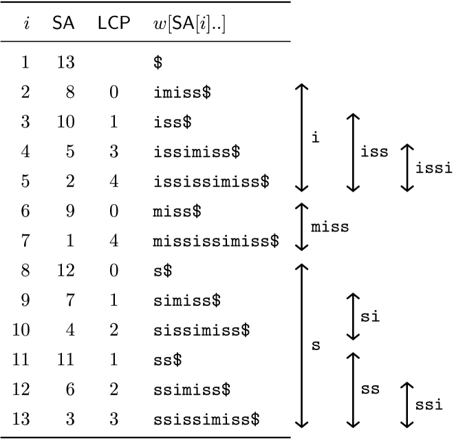
Figure 1: $\mathsf{SA}$ and $\mathsf{LCP}$ of mississimiss$ (left), and its LCP-intervals (right).

Using these, we can enumerate all right-maximal repeats $\alpha$ of $w$ with the sorted array $\mathsf{Idx}_{\alpha}$ of the starting positions of the occurrences of $\alpha$ in $O({n^{2}})$ time, as we will explain below. Right-maximal repeats are known to have a one-to-one correspondence with the concept called LCP-intervals [2, 23]. An LCP-interval discovered by Abouelhoda et al. [2] is intuitively an index interval $[u,v]$ of $\mathsf{SA}$ that cannot be extended without changing the longest common prefix of its corresponding suffixes. We call the length of the longest common prefix LCP-length. The right side of Figure˜1 shows an example of LCP-intervals.

1 $push(\langle 0,\bot\rangle);\;\;\mathsf{LCP}[n+1]\leftarrow 0$

2 for $i\leftarrow 2$ to $n$ do

3    if $\mathsf{LCP}[i+1]>top.lcp$ then  $push(\langle\mathsf{LCP}[i+1],\{\mathsf{SA}[i]\})$

4    else if $\mathsf{LCP}[i+1]=top.lcp$ then

5       if $top.lcp\neq 0$ then insert $\mathsf{SA}[i]$ into $top.\mathsf{Idx}$

6      

7    else

8       insert $\mathsf{SA}[i]$ into $top.\mathsf{Idx}$

9       while $\mathsf{LCP}[i+1]<top.lcp$ do

10          $rmrep\leftarrow pop;\;\;process(rmrep)$

11          if $\mathsf{LCP}[i+1]\leq top.lcp$ then

12             if $top.lcp\neq 0$ then merge $rmrep.\mathsf{Idx}$ into $top.\mathsf{Idx}$

13            

14          else  $push(\langle\mathsf{LCP}[i+1],rmrep.\mathsf{Idx}\rangle)$

15         

16      

17   

Algorithm 6 EnumRM (adapted from Algorithm 4.4 in [2])

We show the enumeration subroutine used in our algorithm. [2] showed an $O({n})$-time enumeration algorithm for right-maximal repeats. By slightly modifying this, we obtain an $O({n^{2}})$-time algorithm EnumRM that enumerates each right-maximal repeat $\alpha$ with the sorted array $\mathsf{Idx}_{\alpha}$ of all starting positions of the occurrences of $\alpha$.

We explain in detail how the algorithm works. Algorithm˜6 shows the pseudocode. The algorithm uses a stack to manage the visiting LCP-intervals. An LCP-interval $I$ being visited is represented by the pair $\langle lcp,\mathsf{Idx}\rangle$ consisting of the LCP-length $lcp$ of $I$ and the array $\mathsf{Idx}$ representing $\{\mathsf{SA}[j]\mid j\in I\text{ and }j\leq i\}$. Initially, the stack has $\langle 0,\bot\rangle$. Next, the algorithm repeats the following steps for $i=2,3,\dots,n$. Let $top=\langle lcp,\mathsf{Idx}\rangle$ denote the pair at the top of the stack. We write $I_{top}$ for the LCP-interval represented by $top$.

In each iteration of the for-loop, the algorithm first compares $lcp$ with $\mathsf{LCP}[i+1]$. We assume $\mathsf{LCP}[n+1]=0$. (1) If $\mathsf{LCP}[i+1]>lcp$, it pushes $\langle\mathsf{LCP}[i+1],\{\mathsf{SA}[i]\}\rangle$ into the stack, because index $i$ is at the left end of an LCP-interval whose LCP-length is greater than $lcp$. (2) If $\mathsf{LCP}[i+1]=lcp$ and the stack has no LCP-interval, it inserts $\mathsf{SA}[i]$ into $\mathsf{Idx}$ while preserving the ascending order, because index $i$ belongs to the LCP-interval $I_{top}$. (3) If $\mathsf{LCP}[i+1]<lcp$, it first inserts $\mathsf{SA}[i]$ into $\mathsf{Idx}$ because index $i$ is at the right end of $I_{top}$. Then, it pops all LCP-intervals whose right end is at $i$ while passing each popped entry $rmrep$ to a placeholder function $process$. A subtle point lies in the relationship between the popped LCP-interval and the one that was directly beneath it on the stack (see Theorem 4.3 of [2] for details). Depending on this relationship, $\mathsf{Idx}$ of $rmrep$ must be merged while preserving the ascending order or pushed as a part of a new LCP-interval accordingly.

For example, the algorithm enumerates the right-maximal repeats of mississimiss$ in the order $\langle 4,[2,5]\rangle\to\langle 3,[2,5,10]\rangle\to\langle 1,[2,5,8,10]\rangle\to\langle 4,[1,9]\rangle\to\langle 2,[4,7]\rangle\to\langle 3,[3,6]\rangle\to\langle 2,[3,6,11]\rangle\to\langle 1,[3,4,6,7,11,12]\rangle$ (see Figure˜1). The algorithm runs in $O({n^{2}})$ time because each step of (1)(2)(3) takes $O({n})$ time, and each is executed at most $O({n})$ times. The space complexity is $O({n})$.

Appendix B Omitted Proofs

Proof B.1 (Proof of Lemma˜3.2).

Immediate from Lemma˜3.16 and Lemma˜3.21.

Proof B.2 (Proof of Lemma˜3.5).

Immediate from the definition of $\Delta$.

Proof B.3 (Proof of Proposition˜3.6).

It suffices to prove the statement of the proposition with “line 1” replaced by “line 1.” We prove by induction on $j$. We write $J^{\prime}_{j}$ for $\{j^{\prime}\in[1,|\mathsf{Idx}_{\alpha}|]\mid i_{j^{\prime}}+|\alpha|\leq i_{j}\text{ and }w[..i_{j^{\prime}}-1]\in L(e_{0})\}$ and $S_{j}$ for $\bigcup_{j^{\prime}\in J^{\prime}_{j}}\Delta(\operatorname{cl_{\varepsilon}}(q_{0}),w[i_{j^{\prime}}+|\alpha|,i_{j}-1])$. We show $S=S_{j}$ right after line $8$ in the iteration with $i_{next}=i_{j}$.

• Case $j=1$: Because $i_{que}=\bot$, the if statement in lines 4 to 8 is skipped and $S=\emptyset$ holds when it reaches line 9. On the other hand, $J^{\prime}_{1}=\emptyset$ because no $\alpha$ occurs before the $\alpha$ at $i_{1}$. Therefore, $S=S_{1}=\emptyset$.

• Case $j-1\to j$: By the induction hypothesis, we have $J^{\prime}_{j-1}=\{j^{\prime}\in[1,|\mathsf{Idx}_{\alpha}|]\mid i_{j^{\prime}}+|\alpha|\leq i_{j-1}\text{ and }w[..i_{j^{\prime}}-1]\in L(e_{0})\}$ and $S=S_{j-1}$ when it reaches line $9$ in the iteration with $i_{next}=i_{j-1}$. At line 10, $i_{prev}=i_{j-1}$ holds. Let $J^{\prime}_{j-1,j}$ denote $\{j^{\prime}\mid i_{j-1}\leq i_{j^{\prime}}+|\alpha|<i_{j}\text{ and }w[..i_{j^{\prime}}-1]\in L(e_{0})\}$. Observe that $J^{\prime}_{j}=J^{\prime}_{j-1}\cup J^{\prime}_{j-1,j}$. From the assumption that $\alpha$ is a nonoverlapping repeat, $J^{\prime}_{j-1,j}$ is either $\emptyset$ or $\{j-1\}$. We consider two cases.

  • Case $\mathsf{Pre}[i_{prev}-1]=\mathbf{true}$: In this case, $e_{0}$ matches $w[..i_{j-1}-1]$. Therefore, $J^{\prime}_{j-1,j}=\{j-1\}$. At line 10, $i_{que}$ becomes $i_{j-1}+|\alpha|-1$. Then, $i_{next}$ becomes $i_{j}$ at line 3. Now, $i_{que}\neq\bot$ and the algorithm enters the for-loop at line 5. We further divide the case into two.

    • Case $S=\emptyset$: In this case, we have $J^{\prime}_{j-1}=\emptyset$. Lines 6 and 7 are skipped until $i$ becomes $i_{que}=i_{j-1}+|\alpha|-1$. When $i=i_{que}$, the algorithm injects $\operatorname{cl_{\varepsilon}}(q_{0})$ into $S$ at line 7 and starts an NFA simulation on $w[i_{j-1}+|\alpha|..i_{j}-1]$. Thus, right after line 8, $S=\Delta(\operatorname{cl_{\varepsilon}}(q_{0}),w[i_{j-1}+|\alpha|..i_{j}-1])$ holds. Therefore, $J^{\prime}_{j}=J^{\prime}_{j-1,j}=\{j-1\}$ and $S=S_{j}$.

    • Case $S\neq\emptyset$: After the for-loop at lines 5 to 7 is executed, $S$ becomes

      $$\Delta(\Delta(S_{j-1},w[i_{j-1}..i_{j-1}+|\alpha|-1])\cup\operatorname{cl_{\varepsilon}}(q_{0}),w[i_{j-1}+|\alpha|..i_{j}-1]).$$

      By the induction hypothesis, $S=\Delta(\Delta(\bigcup_{j^{\prime}\in J^{\prime}_{j-1}}\Delta(\operatorname{cl_{\varepsilon}}(q_{0}),w[i_{j^{\prime}}+|\alpha|..i_{j-1}-1]),w[i_{j-1}..i_{j-1}+|\alpha|-1])\cup\operatorname{cl_{\varepsilon}}(q_{0}),w[i_{j-1}+|\alpha|..i_{j}-1])$. By Lemma˜3.5, this is equal to $\bigcup_{j^{\prime}\in J^{\prime}_{j-1}\cup\{j-1\}}\Delta(\operatorname{cl_{\varepsilon}}(q_{0}),w[i_{j^{\prime}}+|\alpha|..i_{j}-1])$. We have $J^{\prime}_{j}=J^{\prime}_{j-1}\cup\{j-1\}$. Therefore, $S=S_{j}$.

  • Case $\mathsf{Pre}[i_{prev}-1]=\mathbf{false}$: In this case, $e_{0}$ does not match $w[..i_{j-1}-1]$ and $J^{\prime}_{j-1,j}=\emptyset$. At line 3, $i_{next}$ becomes $i_{j}$. We further divide the case into two.

    • Case $i_{que}=\bot$: In this case, we have $S=\emptyset$. The if statement at lines 4 to 8 is skipped and $S=S_{j-1}$ holds right after line 8. Because $J^{\prime}_{j}=J^{\prime}_{j-1}=\emptyset$, $S=S_{j}$ holds.

    • Case $i_{que}\neq\bot$: After the for-loop at lines 5 to 7 is executed, $S$ becomes

      $$\Delta(S_{j-1},w[i_{j-1}..i_{j}-1]).$$

      By Lemma˜3.5 and the induction hypothesis, $S=\Delta(\bigcup_{j^{\prime}\in J^{\prime}_{j-1}}\Delta(\operatorname{cl_{\varepsilon}}(q_{0}),w[i_{j^{\prime}}+|\alpha|..i_{j-1}-1]),w[i_{j-1}..i_{j}-1])=\bigcup_{j^{\prime}\in J^{\prime}_{j-1}}\Delta(\operatorname{cl_{\varepsilon}}(q_{0}),w[i_{j^{\prime}}+|\alpha|..i_{j}-1])$ holds. Because $J^{\prime}_{j}=J^{\prime}_{j-1}$, we have $S=S_{j}$.

Proof B.4 (Proof of Lemma˜3.7).

Let $i_{1}<i_{2}<\cdots$ be the positions in $\mathsf{Idx}_{\alpha}$. Suppose that $\textnormal{{Match1}}(\alpha)$ returns $\mathbf{true}$. From the definition of the algorithm and by Proposition˜3.6, $\alpha\in L(e)$ and there exist $i_{j^{\prime}},i_{j}\in\mathsf{Idx}_{\alpha}$ such that (1) $w[..i_{j^{\prime}}-1]\in L(e_{0})$, (2) $i_{j^{\prime}}+|\alpha|<i_{j}$, (3) $\Delta(\operatorname{cl_{\varepsilon}}(q_{0}),w[i_{j^{\prime}}+|\alpha|..i_{j}-1])\cap F\neq\emptyset$ and (4) $w[i_{j}+|\alpha|..]\in L(e_{2})$. Therefore, $e$ matches $\alpha$ and $r_{\alpha}$ matches $w$. The other direction follows in the same manner.

Proof B.5 (Proof of Proposition˜3.10).

The proof follows similarly to Proposition˜3.6.

Proof B.6 (Proof of Lemma˜3.11).

Recall that $I=\{i\in[i_{beg},i_{end}]\mid w[i_{end}-|\alpha|+1..i]\in L(e)\text{ and }w[i+1..]\in L(e_{2})\}$. For every $i\in[i_{beg},i_{end}]$, we write $I_{\leq i}$ for $\{i^{\prime}\in I\mid i^{\prime}\leq i\}$. Because the statement easily holds when $i_{beg}=i_{end}$, we assume $i_{beg}\leq i_{end}-1$ in what follows. We prove the following statement by induction:

Suppose that $i_{beg}\leq i_{end}-1$. Every time line 3 has been executed at an iteration with $i\in[i_{beg},i_{end}-1]$, $T=\bigcup_{i^{\prime}\in I_{\leq i}}\Delta(\operatorname{cl_{\varepsilon}}(q_{0}),w[i^{\prime}+1..i+1])$. The base case when $i=i_{beg}$ is obvious. Suppose that the step $i-1$ of the for-loop has finished, and line 4 has been executed. By the induction hypothesis, $T=\bigcup_{i^{\prime}\in I_{\leq i-1}}\Delta(\operatorname{cl_{\varepsilon}}(q_{0}),w[i^{\prime}+1..i])$. In step $i$, we consider two cases.

• Case $i\in I$: Observe that $I_{\leq i}=I_{\leq i-1}\cup\{i\}$. In this case, the algorithm injects $\operatorname{cl_{\varepsilon}}(q_{0})$ into $T$ at line 3. Then, immediately after line 4 has been executed, $T$ becomes $\Delta(\bigcup_{i^{\prime}\in I_{\leq i-1}}\Delta(\operatorname{cl_{\varepsilon}}(q_{0}),w[i^{\prime}+1..i])\cup\operatorname{cl_{\varepsilon}}(q_{0}),w[i+1])$. By Lemma˜3.5, this is equal to $\bigcup_{i^{\prime}\in I_{\leq i}}\Delta(\operatorname{cl_{\varepsilon}}(q_{0}),w[i^{\prime}+1..i+1])$.

• Case $i\notin I$: Observe that $I_{\leq i}=I_{\leq i-1}$. In this case, the if statement at line 3 is skipped. If $T=\emptyset$ right after line 3, then $I_{\leq i-1}$ is also empty, which implies $I_{\leq i}=\emptyset$, and thus the statement holds. Otherwise, immediately after line 4 has been executed, $T$ becomes $\Delta(\bigcup_{i^{\prime}\in I_{\leq i-1}}\Delta(\operatorname{cl_{\varepsilon}}(q_{0}),w[i^{\prime}+1..i]),w[i+1])$. By Lemma˜3.5, this is equal to $\bigcup_{i^{\prime}\in I_{\leq i}}\Delta(\operatorname{cl_{\varepsilon}}(q_{0}),w[i^{\prime}+1..i+1])$.

Finally, we divide the cases into two for the last iteration of the for-loop.

• Case $i_{end}\in I$: after line 3 is executed, $T$ becomes $\bigcup_{i^{\prime}\in I_{\leq i_{end}-1}}\Delta(\operatorname{cl_{\varepsilon}}(q_{0}),w[i^{\prime}+1..i_{end}])\cup\operatorname{cl_{\varepsilon}}(q_{0})=\bigcup_{i^{\prime}\in I_{\leq i_{end}}}\Delta(\operatorname{cl_{\varepsilon}}(q_{0}),w[i^{\prime}+1..i_{end}])$.

• Case $i_{end}\notin I$: similarly to the above case.

Proof B.7 (Proof of Lemma˜3.16).

Let $i_{1}<i_{2}<\cdots$ be the positions in $\mathsf{Idx}_{\alpha}$. Suppose that $\mathsf{Que}\neq\bot$ holds for the first time in an iteration with $i_{next}=i_{j_{0}}$. For each $i_{j}\geq i_{j_{0}}$, right after executing the iteration with $i_{next}=i_{j}$, $\mathsf{Que}$ represents $\{i_{j^{\prime}}+|\alpha|-1\mid i_{j^{\prime}}\leq i_{j}\leq i_{j^{\prime}}+|\alpha|-1\land w[..i_{j^{\prime}}-1]\in L(e_{0})\}$ in a sorted order. We prove by induction on $j$. The base case $j=j_{0}$ easily holds. At the beginning of the iteration with $i_{next}=i_{j}$, $\mathsf{Que}$ represents $\{i_{j^{\prime}}+|\alpha|-1\mid i_{j^{\prime}}\leq i_{j-1}\leq i_{j^{\prime}}+|\alpha|-1\land w[..i_{j^{\prime}}-1]\in L(e_{0})\}$. Then, right after completing the execution of the for-loop in lines 5 to 9, $\mathsf{Que}$ becomes $\{i_{j^{\prime}}+|\alpha|-1\mid i_{j^{\prime}}\leq i_{j-1}\land i_{j}\leq i_{j^{\prime}}+|\alpha|-1\land w[..i_{j^{\prime}}-1]\in L(e_{0})\}$. We divide the case into two.

• Case $w[..i_{j}-1]\in L(e_{0})$: The algorithm enqueues $i_{j}+|\alpha|-1$ into $\mathsf{Que}$ at line 15. Therefore, the claim holds for $i_{j}$.

• Case $w[..i_{j}-1]\notin L(e_{0})$: The if statement in lines 13 to 15 is skipped. Therefore, the claim holds for $i_{j}$.

Every time line 4 is reached at iteration with $i_{next}=i_{j}$, $\mathcal{S}[l]=\bigcup_{j^{\prime}\in J^{\prime}}\Delta(q_{l},w[i_{j^{\prime}}+|\alpha|,i_{j}-1])$ where $J^{\prime}=\{j^{\prime}\in[1,|\mathsf{Idx}_{\alpha}|]\mid i_{j^{\prime}}+|\alpha|\leq i_{j}\text{ and }w[..i_{j^{\prime}}-1]\in L(e_{0})\}$. With the above claim, the proof follows in the same way as for Proposition˜3.6.

The lemma can be proved in the same way as Lemma˜3.12, using the above claim and Lemma˜3.11.

Proof B.8 (Proof of Proposition˜3.20).

The proof follows similarly to Lemma˜3.11.

Proof B.9 (Proof of Lemma˜3.21).

We prove only one direction. Let $i_{1}<i_{2}<\cdots$ be the positions in $\mathsf{Idx}_{\alpha}$. Suppose that there is a prefix $\beta=\alpha[..k]$ of $\alpha$ and positions $i_{j}$ and $i_{j^{\prime}}$ such that (1) $\overrightarrow{\beta}=\alpha$, (2) $\beta\in L(e)$, (3) $i_{j}+k\leq i_{j^{\prime}}$, (4) $w[..i_{j}-1]\in L(e_{0})$, (5) $w[i_{j}+k..i_{j^{\prime}}-1]\in L(e_{1})$, (6) $w[i_{j^{\prime}}+k..]\in L(e_{2})$ and (7) the $\beta$’s are not $\alpha$-separable, i.e., $i_{j^{\prime}}\leq i_{j}+|\alpha|-1$.

We claim that $i_{j^{\prime}}=f(i_{j})$. Otherwise, $i_{j}<i_{j^{\prime}}<f(i_{j})$ holds, and by Lemma˜3.18, $\overrightarrow{w[i_{j}..i_{j^{\prime}}-1]}\neq\alpha$, which contradicts (1) and (3). In what follows, we show that the algorithm returns $\mathbf{true}$ at an iteration with $i_{next}=i_{j}$. We first check the guard condition at line 5. Observe that $f_{next}=f(i_{j})$. Among the three conditions, the first two clearly hold. In fact, the third condition also holds. When $j=1$, $f_{prev}=0$ and it trivially holds. Assume, to the contrary, that it does not hold for $j\geq 2$. In this case, we have $f_{prev}=f(i_{j-1})$ and $f(i_{j-1})=f(i_{j})$. Then, the occurrence of $\alpha$ at $i_{j-1}$ contains $\beta=w[i_{j}..i_{j}+k-1]=w[i_{j-1}..i_{j-1}+k-1]$ twice, violating Lemma˜3.14.

By Proposition˜3.20, at line 5, $S$ becomes $\bigcup_{i\in I}\Delta(\operatorname{cl_{\varepsilon}}(q_{0}),w[i+1..f(i_{j})-1])$ where $I=\{i\in[\max\{i_{j},f(i_{j-1})\},f(i_{j})-1]\mid w[i_{j}..i]\in L(e)\text{ and }w[f(i_{j})+i-i_{j}+1]\in L(e_{2})\}$. Here, we regard $f(i_{j-1})=0$ when $j=1$. It suffices to show that $i_{j}+k-1\geq\max\{i_{j},f(i_{j-1})\}$. If $i_{j}\geq f(i_{j-1})$, it trivially holds, so we may assume $j\geq 2$ and $i_{j}<f(i_{j-1})$. Suppose that $f(i_{j-1})>i_{j}+k-1$. Let $\beta^{\prime}$ be $w[i_{j}..f(i_{j-1})-1]$, which is equal to $\beta$ or longer. By Lemma˜3.18, $\overrightarrow{\beta^{\prime}}\neq\alpha$ holds. This is a contradiction.

References

- [1] WhyRE2. https://github.com/google/re2/wiki/WhyRE2 (Accessed: 2024-12-14).
- [2] Mohamed Ibrahim Abouelhoda, Stefan Kurtz, and Enno Ohlebusch. Replacing suffix trees with enhanced suffix arrays. Journal of discrete algorithms, 2(1):53–86, 2004.
- [3] Alfred V. Aho. Algorithms for finding patterns in strings, page 255–300. MIT Press, Cambridge, MA, USA, 1991.
- [4] Dana Angluin. Finding patterns common to a set of strings. In Proceedings of the eleventh annual ACM Symposium on Theory of Computing, pages 130–141, 1979.
- [5] Arturs Backurs and Piotr Indyk. Which regular expression patterns are hard to match? In 2016 IEEE 57th Annual Symposium on Foundations of Computer Science (FOCS), pages 457–466. IEEE, 2016.
- [6] Aurèle Barrière and Clément Pit-Claudel. Linear matching of JavaScript regular expressions. Proceedings of the ACM on Programming Languages, 8(PLDI):1336–1360, 2024.
- [7] Martin Berglund, Brink van Der Merwe, and Steyn van Litsenborgh. Regular expressions with lookahead. Journal of universal computer science (Online), 27(4):324–340, 2021.
- [8] Philip Bille. New algorithms for regular expression matching. In International Colloquium on Automata, Languages, and Programming, pages 643–654. Springer, 2006.
- [9] Philip Bille and Martin Farach-Colton. Fast and compact regular expression matching. Theoretical Computer Science, 409(3):486–496, 2008.
- [10] Philip Bille and Inge Li Gørtz. Sparse regular expression matching. In Proceedings of the 2024 Annual ACM-SIAM Symposium on Discrete Algorithms (SODA), pages 3354–3375. SIAM, 2024.
- [11] Philip Bille and Mikkel Thorup. Faster regular expression matching. In Automata, Languages and Programming: 36th International Colloquium, ICALP 2009, Rhodes, Greece, July 5-12, 2009, Proceedings, Part I 36, pages 171–182. Springer, 2009.
- [12] Maxime Crochemore. Transducers and repetitions. Theoretical Computer Science, 45:63–86, 1986.
- [13] Maxime Crochemore and Renaud Vérin. Direct construction of compact directed acyclic word graphs. In Combinatorial Pattern Matching: 8th Annual Symposium, CPM 1997, pages 116–129. Springer, 1997.
- [14] James C Davis, Christy A Coghlan, Francisco Servant, and Dongyoon Lee. The impact of regular expression denial of service (ReDoS) in practice: an empirical study at the ecosystem scale. In Proceedings of the 2018 26th ACM joint meeting on european software engineering conference and symposium on the foundations of software engineering, pages 246–256, 2018.
- [15] James C Davis, Francisco Servant, and Dongyoon Lee. Using selective memoization to defeat regular expression denial of service (ReDoS). In 2021 IEEE symposium on security and privacy (SP), pages 1–17. IEEE, 2021.
- [16] Andrzej Ehrenfreucht and Grzegorz Rozenberg. Finding a homomorphism between two words in NP-complete. Information Processing Letters, 9(2):86–88, 1979.
- [17] Henning Fernau, Florin Manea, Robert Mercaş, and Markus L Schmid. Pattern matching with variables: efficient algorithms and complexity results. ACM Transactions on Computation Theory (TOCT), 12(1):1–37, 2020.
- [18] Henning Fernau and Markus L Schmid. Pattern matching with variables: a multivariate complexity analysis. Information and Computation, 242:287–305, 2015.
- [19] Henning Fernau, Markus L Schmid, and Yngve Villanger. On the parameterised complexity of string morphism problems. Theory of Computing Systems, 59(1):24–51, 2016.
- [20] Dominik D Freydenberger and Markus L Schmid. Deterministic regular expressions with back-references. Journal of Computer and System Sciences, 105:1–39, 2019.
- [21] Hiroya Fujinami and Ichiro Hasuo. Efficient matching with memoization for regexes with look-around and atomic grouping. In European Symposium on Programming, pages 90–118. Springer, 2024.
- [22] Zvi Galil. Open problems in stringology. In Alberto Apostolico and Zvi Galil, editors, Combinatorial Algorithms on Words, pages 1–8. Springer, 1985.
- [23] Dan Gusfield. Algorithms on strings, trees and sequences: computer science and computational biology. Cambridge University Press, 1997.
- [24] W. Daniel Hillis and Guy L. Steele. Data parallel algorithms. Commun. ACM, 29(12):1170–1183, 1986. doi:10.1145/7902.7903.
- [25] Shunsuke Inenaga, Hiromasa Hoshino, Ayumi Shinohara, Masayuki Takeda, and Setsuo Arikawa. On-line construction of symmetric compact directed acyclic word graphs. In Proceedings Eighth Symposium on String Processing and Information Retrieval, pages 96–110. IEEE, 2001.
- [26] Toru Kasai, Gunho Lee, Hiroki Arimura, Setsuo Arikawa, and Kunsoo Park. Linear-time longest-common-prefix computation in suffix arrays and its applications. In Proceedings of the 12th Annual Symposium on Combinatorial Pattern Matching, CPM ’01, page 181–192. Springer-Verlag, 2001.
- [27] Richard E. Ladner and Michael J. Fischer. Parallel prefix computation. J. ACM, 27(4):831–838, 1980. doi:10.1145/322217.322232.
- [28] Felipe A Louza, Simon Gog, and Guilherme P Telles. Construction of fundamental data structures for strings. Springer, 2020.
- [29] Michael G Main and Richard J Lorentz. Linear time recognition of squarefree strings. In Combinatorial Algorithms on Words, pages 271–278. Springer, 1985.
- [30] Konstantinos Mamouras and Agnishom Chattopadhyay. Efficient matching of regular expressions with lookaround assertions. Proceedings of the ACM on Programming Languages, 8(POPL):2761–2791, 2024.
- [31] Takayuki Miyazaki and Yasuhiko Minamide. Derivatives of regular expressions with lookahead. Journal of Information Processing, 27:422–430, 2019.
- [32] Akimasa Morihata. Translation of regular expression with lookahead into finite state automaton. Computer Software, 29(1):147–158, 2012.
- [33] Gene Myers. A four russians algorithm for regular expression pattern matching. Journal of the ACM (JACM), 39(2):432–448, 1992.
- [34] Kazuyuki Narisawa, Hideharu Hiratsuka, Shunsuke Inenaga, Hideo Bannai, and Masayuki Takeda. Efficient computation of substring equivalence classes with suffix arrays. Algorithmica, 79:291–318, 2017.
- [35] Enno Ohlebusch. Bioinformatics algorithms: sequence analysis, genome rearrangements, and phylogenetic reconstruction. Oldenbusch Verlag, 2013.
- [36] Mathieu Raffinot. On maximal repeats in strings. Information Processing Letters, 80(3):165–169, 2001.
- [37] Daniel Reidenbach and Markus L Schmid. A polynomial time match test for large classes of extended regular expressions. In Implementation and Application of Automata: 15th International Conference, CIAA 2010, Winnipeg, MB, Canada, August 12-15, 2010. Revised Selected Papers 15, pages 241–250. Springer, 2011.
- [38] Markus L Schmid. Regular expressions with backreferences: polynomial-time matching techniques. URL: https://arxiv.org/abs/1903.05896.
- [39] Markus L Schmid. A note on the complexity of matching patterns with variables. Information Processing Letters, 113(19-21):729–733, 2013.
- [40] Markus L Schmid. Characterising REGEX languages by regular languages equipped with factor-referencing. Information and Computation, 249:1–17, 2016.
- [41] Ryoma Sin’ya, Kiminori Matsuzaki, and Masataka Sassa. Simultaneous finite automata: An efficient data-parallel model for regular expression matching. In Proceedings of the 2013 42nd International Conference on Parallel Processing, page 220–229. IEEE Computer Society, 2013. doi:10.1109/ICPP.2013.31.
- [42] Henry Spencer. A regular-expression matcher, page 35–71. Academic Press Professional, Inc., USA, 1994.
- [43] Masayuki Takeda, Tetsuya Matsumoto, Tomoko Fukuda, and Ichiro Nanri. Discovering characteristic expressions in literary works. Theoretical Computer Science, 292(2):525–546, 2003.
- [44] Ken Thompson. Programming techniques: regular expression search algorithm. Communications of the ACM, 11(6):419–422, 1968.