Multi-tracer beyond linear theory

Abstract

The multi-tracer (MT) technique has been shown to outperform single-tracer analyses in the context of galaxy clustering. In this paper, we conduct a series of Fisher analyses to further explore MT information gains within the framework of non-linear bias expansion. We examine how MT performance depends on the bias parameters of the subtracers, showing that directly splitting the non-linear bias generally leads to smaller error bars in $A_{s}$, $h$, and $\omega_{\rm cdm}$ compared to a simple split in $b_{1}$. This finding opens the door to identifying subsample splits that do not necessarily rely on very distinct linear biases. We discuss different total and subtracer number density scenarios, as well as the possibility of splitting into more than two tracers. Additionally, we consider how different Fingers-of-God suppression scales for the subsamples can be translated into different $k_{\rm max}$ values. Finally, we present forecasts for ongoing and future galaxy surveys.

1 Introduction

In light of the large datasets provided by galaxy surveys [1, 2, 3, 4, 5, 6, 7, 8], how can we maximize the amount of information extracted from them? Attempts to extract additional information include using alternative statistics [9, 10, 11, 12, 13, 14, 15, 16] or considering field-level analysis [17]. In this work, we focus on the multi-tracer (MT) approach as a tool to extract more information from galaxy clustering. The multi-tracer method has been extensively discussed as a way to improve the measurement of primordial non-Gaussianities and redshift-space distortions [18, 19, 20, 21, 22, 23, 24, 25, 26, 27, 28, 29, 30, 31, 32, 33, 34, 35, 36, 37, 38, 39, 40, 41, 42, 43]. Moreover, MT serves as a central tool for the SPHEREx collaboration in improving their results on primordial non-Gaussianities [7, 44].

Most MT analyses have been based on linear theory and the cosmic-variance cancellation argument, finding that multi-tracer techniques generally perform better when there is a larger difference in their linear bias parameters. This approach relies on the non-trivial task of identifying two samples that have some redshift overlap while having different linear bias values. The references [45, 46] (see also [47, 48]) have extended the former analysis to include non-linear scales by considering additional bias coefficients and loop calculations within the effective field theory (EFT) of large-scale structure framework [49, 50, 51, 52, 53, 54, 55, 56, 57, 58, 59, 60, 61] and the large-scale bias expansion [62]. Their work shows that multi-tracer improvements can extend beyond cosmic variance cancellation: the correlation matrix of the MT basis is more diagonal compared to that of single-tracer (ST) analyses, effectively breaking degeneracies between different bias coefficients and cosmological parameters.

In this work, we extend the study of [45, 46] conducing a series of Fisher analysis that allows us to easily explore different MT scenarios in the context of non-linear galaxy clustering. Instead of splitting the samples via a feature such as color or mass, we study the direct dependence of the MT gains as a function of the direct difference in their (linear and non-linear) bias parameters. We find that detecting samples with distinct non-linear bias coefficients leads to comparable (and often better) results than a simple split in the linear bias. Using separate-Universe based relations, we investigate the possibility of finding tracers with different non-linear bias parameter. Despite finding that it is relatively difficult to have tracers with different non-linear bias coefficients in the most vanilla scenario, it is shown that assembly bias can help to find tracers with very distinct $b_{\mathcal{G}_{2}}$ [63]. Next, we study the information budget encoded in MT at both linear and non-linear orders. In the non-linear scenario, the cross-spectra adds an important piece of information compared to the linear MT. We also find the linear case to be way more dependent on the assumption of no cross-stochasticity between the tracers. When considering the EFT modeling, the MT leads to significant better results even when including the cross-stochastic contribution, in tandem with the results of [45, 46].

Moreover, we consider for the first time a MT non-linear galaxy clustering analysis with more than two tracers. We show that, for realistic survey specifications, two tracers is the optimal number of tracers. Furthermore, we study the dependence of the MT information gain on the total tracer number density. We find that, while the MT gains are limited to the very high number density case, when modeling with non-linear bias coefficients MT overtakes ST already for number densities of $10^{-4}h^{3}$Mpc^-3. We also consider a non-balanced split between the two subsamples, in which one of the samples is denser compared to the other. We find that most of the MT gains are present even in the case in which one of the samples correspond to $\sim 10\%$ of the total sample. This result makes easier the task of finding two samples with different bias parameters, since one can restrict to the $10\%$ less homogeneous subsample. We also discuss how MT can be used to select subsamples with different Fingers-of-God (FoG) suppression scale, such that one could use different scale cuts for different tracers. Finally, we forecast the sensitivity of current and future galaxy surveys.

The structure of this paper is the following. In Sec. 2 we construct discuss the bias expansion for multi-tracer and the details of the Fisher analysis performed in this work. We present the results in terms of the bias split in Sec. 3. Next, in Sec. 4 we discuss the optimal number of tracers and the dependence on the total and subtracer number density. Sec. 5 develops on the FoG suppression for the different subsample. We present forecasts for distinct galaxy surveys in Sec. 6 and conclude in Sec. 7. We have dedicated appendices for discussing the stability of the Fisher derivatives in App. A, the dependence on the fiducial bias choice in App. B and for extra plots in App. C.

2 Prerequisites

In this section, we review the large-scale bias expansion and its extension to multi-tracer in Sec. 2.1. Next, we describe the Fisher information in Sec. 2.2. In Sec. 2.3, we present the setup for the Fisher analysis.

2.1 The large-scale bias expansion

We start by considering a tracer $T$ with density $\rho^{T}(\bm{x},z)$ and an average background density $\bar{\rho}^{T}(z)$ in the redshift $z$. The bias expansion [62] consists of expanding its overdensity

$$\delta^{T}(\bm{x},z)=\frac{\rho^{T}(\bm{x},z)}{\bar{\rho}^{T}(z)}-1=\sum_{\mathcal{O}}b_{\mathcal{O}}^{T}(z)\mathcal{O}(\bm{x},z)+\epsilon^{T}(\bm{x},z)\,,$$ (2.1)

in terms of the most general basis of operators

$$\mathcal{O}\in\left\{\delta,\delta^{2},\mathcal{G}_{2}[\Phi_{g}],\Gamma_{3}[\Phi_{g},\Phi_{v}],\nabla^{2}\delta\right\}\,,$$ (2.2)

and their respective bias parameters $b_{\mathcal{O}}^{T}(z)$, with $b_{1}=b_{\delta}$. These operators are constructed as functions of the gravitational and velocity potentials $\Phi_{g}$ and $\Phi_{v}$, respectively. In this work, we consider only the operators in Eq. (2.2) that contribute to the one-loop power spectrum. Another central element in the bias expansion is the presence of a stochastic component $\epsilon^{T}$ [65, 66], which leads to corrections of small-scale modes onto large scales, such as the shot-noise term.

The auto power spectrum of the tracer $T$ is therefore given by

$$P^{TT}(k,z)=\sum_{\mathcal{O}_{\alpha},\mathcal{O}_{\beta}}b_{\mathcal{O}_{\alpha}}^{T}(z)b_{\mathcal{O}_{\beta}}^{T}(z)\mathcal{P}_{\mathcal{O}_{\alpha},\mathcal{O}_{\beta}}(k,z)+P_{\rm c.t.}^{TT}(k,z)+P_{\rm stoch}^{TT}(k,z)\,,$$ (2.3)

where the functions $\mathcal{P}_{\mathcal{O}_{\alpha},\mathcal{O}_{\beta}}$ can be calculated taking contractions of the operators $\mathcal{O}_{\alpha}$ and $\mathcal{O}_{\beta}$ (see e.g. [64] for the form of those operators). The counter-term to the one-loop power spectrum is given by the operator $\nabla^{2}\delta$

$$P_{\rm c.t.}^{TT}(k,z)=-2b^{T}_{\nabla^{2}\delta}(z)b^{T}_{\delta}(z)\frac{k^{2}}{k_{\rm norm}^{2}}P_{\rm L}(z)\,,$$ (2.4)

where $k_{\rm norm}=0.1\,h/$Mpc is a normalization scale chosen such that $b^{T}_{\nabla^{2}\delta}$ is dimensionless and with $P_{\rm L}$ denoting the linear matter power spectrum. The stochastic term is calculated as the contribution of $\epsilon^{T}$ to large-scale modes and can be parametrized (at leading-order in perturbation theory) as a constant and a $k^{2}$ term

$$P_{\rm stoch}^{TT}(k,z)=\frac{1}{\bar{n}_{T}}\left(1+c^{TT}_{0}(z)+c^{TT}_{2}(z)\frac{k^{2}}{k_{\rm norm}^{2}}\right)\,,$$ (2.5)

where $\bar{n}_{T}$ is the number density of the tracer $T$.

The multi-tracer approach consists of splitting the tracer $T$ into (disjoint) sub-tracer samples $t_{i}$ based on specific criteria e.g., the mass of the sample, color, spin or the star formation rate. The total density can then be written as the sum of its parts

$$\rho^{T}(\bm{x},z)=\sum_{t_{i}}\rho^{t_{i}}(\bm{x},z)\,,\quad\textrm{such that}\quad\delta^{T}(\bm{x},z)=\frac{1}{\bar{n}^{T}}\sum_{t_{i}}\bar{n}^{t_{i}}\delta^{t_{i}}(\bm{x},z)\,,$$ (2.6)

with $\bar{n}^{T}=\sum_{t_{i}}\bar{n}^{t_{i}}$. The spectra $P^{t_{i}t_{j}}(k,z)$ for two sub-tracers with overdensities $\delta^{t_{i}}(\bm{x},z)$ and $\delta^{t_{j}}(\bm{x},z)$ can be written as a generalization of Eq. (2.3)

$$P^{t_{i}t_{j}}(k,z)=\sum_{\mathcal{O}_{\alpha},\mathcal{O}_{\beta}}b_{\mathcal{O}_{\alpha}}^{t_{i}}(z)b_{\mathcal{O}_{\beta}}^{t_{j}}(z)\mathcal{P}_{\mathcal{O}_{\alpha},\mathcal{O}_{\beta}}(k,z)+P_{\rm c.t.}^{t_{i}t_{j}}(k,z)+P_{\rm stoch}^{t_{i}t_{j}}(k,z)\,,$$ (2.7)

which includes the auto-spectra of the tracer $t_{i}$ when $j=i$. This is a fundamental point for MT: instead of considering a single species with only a single auto spectrum it breaks this species into sub-tracers also including their cross-correlations [42]. The tracer split can lead to different auto- and cross-spectrum shapes that are otherwise averaged out in the single-tracer auto spectrum. For example, one can see stronger Fingers-of-God (FoG) effects in one of the samples [46]. Altogether, this can help to break the degeneracy between bias, stochastic and cosmological parameters, leading to a more diagonal cross-correlation matrix between these parameters [45, 46]. On the other hand, the tracer split enhances the shot-noise contribution since $(\bar{n}^{t_{i}})^{-1}\geq(\bar{n}^{T})^{-1}$, which can deteriorate the signal-to-noise ratio.

The counter-term for the MT case is

$$P_{\rm c.t.}^{t_{i}t_{j}} = -\left[b^{t_{i}}_{\nabla^{2}\delta}(z)b^{t_{j}}_{\delta}(z)+b^{t_{j}}_{\nabla^{2}\delta}(z)b^{t_{i}}_{\delta}(z)\right]\frac{k^{2}}{k^{2}_{\mathrm{norm}}}P_{\rm L}(z)\;,$$ (2.8)

and the stochastic is given by

$$P_{\rm stoch}^{t_{i}t_{j}}(k,z)=\frac{1}{\sqrt{\bar{n}^{t_{i}}\bar{n}^{t_{j}}}}\left[\delta^{K}_{ij}+c^{t_{i}t_{j}}_{0}(z)+c^{t_{i}t_{j}}_{2}(z)\frac{k^{2}}{k^{2}_{\mathrm{norm}}}\right]\,,$$ (2.9)

where $\delta^{K}_{ij}$ is the Kronecker delta. It is often assumed that $P_{\rm stoch}^{t_{i}t_{j}}(k,z)=0$ for $j\neq i$, which implies that the stochastic fields $\epsilon^{t_{i}}$ and $\epsilon^{t_{j}}$ do not correlate, as small scale processes for the tracer $i$ are, in principle, independent of those for the tracer $j$. Noise suppression can substantially enhance the information extracted out of galaxy clustering [67]. Despite the cross-noise being relatively small compared to the diagonal part [68], as predicted by the halo model [69], it has been shown that exclusion effects, satellite galaxies [70] and also nonlinearities can enhance correlations on large scales [71]. Previous MT works [45, 46] have found that the inclusion of those terms do not sensibly affect the constraints on cosmological parameters when considering non-linear theory. As we see later, this is a big difference compared to the linear MT results. We discuss the impact of including the cross-stochastic term later in this work.

In redshift space, the power spectrum depends on the angle $\mu=\frac{\hat{z}\cdot\vec{k}}{k}$ measured relative to the line-of-sight direction $\hat{z}$

$$P^{t_{i}{t_{j}}}(k,\mu,z) =Z^{t_{i}}_{1}(k,z)Z^{t_{j}}_{1}(k,z)P_{\rm L}(k,z)+3Z_{1}^{t_{i}}(\bm{k},z)P_{\rm L}(k,z)\int_{\bm{q}}Z_{3}^{t_{j}}(\bm{q},-\bm{q},\bm{k},z)P_{\rm L}(q,z)$$

$$+2\int_{\bm{q}}Z^{t_{i}}_{2}(\bm{q},\bm{k}-\bm{q},z)Z^{t_{j}}_{2}(\bm{q},\bm{k}-\bm{q},z)P_{\rm L}(z,|\bm{k}-\bm{q}|,z)P_{\rm L}(q,z)$$

$$+3Z_{1}^{t_{j}}(\bm{k},z)P_{\rm L}(k,z)\int_{\bm{q}}Z_{3}^{t_{i}}(\bm{q},-\bm{q},\bm{k},z)P_{\rm L}(q,z)+P_{\text{c.t.}}^{{t_{i}}{t_{j}}}(k,\mu,z)+P_{\varepsilon^{t_{i}}\varepsilon^{t_{j}}}(k,\mu,z)\,,$$ (2.10)

where we follow the notation used in [46]. For the complete form of the $Z$ kernels, including their dependence on the bias parameters, see [72, 64]. The counter-term and stochastic power spectrum are given by [46]

$$P_{\rm c.t.}^{{t_{i}}{t_{j}}}(k,\mu,z) =\frac{k^{2}}{k_{\rm norm}^{2}}P_{\rm L}(k,z)\left[Z^{t_{i}}_{1}(k,z)\left(c^{t_{j}}_{{\rm ct},20}(z)+c^{t_{j}}_{{\rm ct},22}(z)\mu^{2}+c^{t_{j}}_{{\rm ct},24}(z)\mu^{4}\right.\right.$$ (2.11)

$$\left.\left.+c^{t_{j}}_{{\rm ct},44}(z)\frac{k^{2}}{k_{\rm norm}^{2}}\mu^{4}+c^{t_{j}}_{{\rm ct},46}(z)\frac{k^{2}}{k_{\rm norm}^{2}}\mu^{6}\right)+{t_{i}}\leftrightarrow{t_{j}}\right]\,,$$

$$P_{\varepsilon^{t_{i}}\varepsilon^{t_{j}}}(k,\mu,z) =\frac{1}{\sqrt{\bar{n}_{t_{i}}\bar{n}}_{t_{j}}}\left[c^{{t_{i}}{t_{j}}}_{\rm st,00}(z)+c^{{t_{i}}{t_{j}}}_{\rm st,20}(z)\frac{k^{2}}{k_{\rm norm}^{2}}+c^{{t_{i}}{t_{j}}}_{\rm st,22}(z)\frac{k^{2}}{k_{\rm norm}^{2}}f(z)\mu^{2}\right]\,.$$ (2.12)

Following [73, 60, 46], we include higher-order terms in $k^{2}$ in the counter-term as a proxy for higher-order contributions to the Fingers-of-God (FoG) effect. We can then expand the power spectrum into multipoles

$$P^{{t_{i}}{t_{j}}}(k,\mu,z)=\sum_{\ell\;{\rm even}}{\cal L}_{\ell}(\mu)P^{{t_{i}}{t_{j}}}_{\ell}(k,z)\,,$$ (2.13)

such that each multipole is given by the projection into Legendre polynomial

$$P^{{t_{i}}{t_{j}}}_{\ell}(k,z)\equiv\frac{2\ell+1}{2}\int_{-1}^{1}d\mu\,{\cal L}_{\ell}(\mu)P^{{t_{i}}{t_{j}}}(k,\mu,z)\,.$$ (2.14)

We use a modified version of CLASS-PT [64], built on top of CLASS [74], to compute these spectra, along with the inbuilt IR-resummation (see [75, 76] for details).

2.2 Fisher analysis

In real space, the Fisher information matrix for a single tracer $T$ is given by

$$F_{\theta_{a}\theta_{b}}^{\rm ST}=\sum_{\alpha,\beta}\frac{\partial}{\partial\theta_{a}}P^{TT}(k_{\alpha})\,\operatorname{Cov}^{-1}_{TT,TT}(k_{\alpha},k_{\beta})\,\frac{\partial}{\partial\theta_{b}}P^{TT}(k_{\beta})\,,$$ (2.15)

where $\bm{\theta}$ is the vector of parameters, and the sum runs over the different discrete wavelength modes $k_{\alpha}$ and $k_{\beta}$. The (marginalized) error in the parameter $\theta_{a}$ is given by the square root of the inverse of the Fisher matrix

$$\sigma_{\theta_{a}}=\sqrt{\left(F^{-1}\right)_{aa}}\,.$$ (2.16)

Moreover, we assume a diagonal Gaussian covariance

$$\operatorname{Cov}_{TT,TT}(k_{\alpha},k_{\beta})=\delta_{\alpha,\beta}^{K}\frac{2}{m_{k_{\alpha}}}\left[P^{TT}(k_{\alpha})\right]^{2}\,,$$ (2.17)

where the shot noise is included in $P^{TT}$ as in Eq. (2.3). Also, $m_{k_{\alpha}}=Vk_{\alpha}^{2}\Delta k/(2\pi^{2})$ is the number of modes, where $V$ is the survey volume and $\Delta k$ is the $k$ bin width of the $k$-bin considered. For extensions of the Gaussian covariance, see [77].

The extension of the Fisher information matrix for a MT set with $N_{\rm Tracers}$ tracers $t_{1},\dots,t_{N_{\rm Tracers}}$ is given by [45] (see also [78])

$$F_{\theta_{a}\theta_{b}}^{\rm MT}=\sum^{N_{\rm Tracers}}_{\begin{subarray}{c}t_{i},t_{j},t_{k},t_{m},\\ {\rm with}\\ i\leq j;k\leq m\end{subarray}}\sum_{\alpha,\beta}\frac{\partial}{\partial\theta_{a}}P^{t_{i}t_{j}}(k_{\alpha})\,\operatorname{Cov}^{-1}_{t_{i}t_{j},t_{k}t_{m}}(k_{\alpha},k_{\beta})\,\frac{\partial}{\partial\theta_{b}}P^{t_{k}t_{m}}(k_{\beta})\,,$$ (2.18)

with the auto and cross-spectra calculated as Eq. (2.7) and the covariance

$$\operatorname{Cov}_{t_{i}t_{j},t_{k}t_{m}}(k_{\alpha},k_{\beta})=\delta_{\alpha,\beta}^{K}\frac{1}{m_{k_{\alpha}}}\left[P^{t_{i}t_{k}}(k_{\alpha})P^{t_{j}t_{m}}(k_{\alpha})+P^{t_{i}t_{m}}(k_{\alpha})P^{t_{j}t_{k}}(k_{\alpha})\right]\,.$$ (2.19)

We also assume that all the tracers overlap within a single redshift bin. Once more, we consider a Gaussian covariance for MT, since we restrict our analysis to relatively large scales $k\leq 0.15\,h/$Mpc where the Gaussian covariance shows good agreement with the covariance measured from simulations [79]. We leave the investigation of the impact of the non-Gaussian covariance on MT for a future project. We discuss the stability of the Fisher derivatives in App. A.

The Gaussian covariance in redshift space can be written using the 3j Wigner symbols as

$$\operatorname{Cov}_{t_{i}t_{j},t_{k}t_{m}}^{\ell\ell^{\prime}}(k_{\alpha},k_{\beta})= \delta_{\alpha,\beta}^{K}\frac{\left(2\ell+1\right)\left(2\ell^{\prime}+1\right)}{m_{k_{\alpha}}}\sum_{\ell_{1}\ell_{2}\ell_{3}}\left(2\ell_{3}+1\right)\left(\begin{array}[]{ccc}\ell_{1}&\ell_{2}&\ell_{3}\\ 0&0&0\end{array}\right)^{2}\left(\begin{array}[]{ccc}\ell&\ell^{\prime}&\ell_{3}\\ 0&0&0\end{array}\right)^{2}$$ (2.24)

$$\qquad\left[\left(-1\right)^{\ell^{\prime}}P_{\ell_{1}}^{t_{i}t_{k}}\left(k_{\alpha}\right)P_{\ell_{2}}^{t_{j}t_{m}}\left(k_{\alpha}\right)+P_{\ell_{1}}^{t_{i}t_{m}}\left(k_{\alpha}\right)P_{\ell_{2}}^{t_{j}t_{k}}\left(k_{\alpha}\right)\right]\,.$$ (2.25)

The Fisher is then given by Eq. (2.18) summing over the monopole, quadrupole and hexadecapole contributions. Notice that the triangle inequality of the 3j Wigner symbols bounds $\ell_{3}$ to $|l_{1}-l_{2}|\leq l_{3}\leq|l_{1}+l_{2}|$. In our analysis we consider only the first three even multipoles of the tracer power spectrum, so that the sums above are all effectively bounded.

2.3 Fisher Setup

For the Fisher analysis, we adopt a Planck 18 cosmology [80], keeping $h,\omega_{\rm cdm}$ and $A_{s}$ free together with the bias parameters and without adding any priors. A realistic tracer split accounts for observed features such as the color, sample mass, star formation rate or local overdensity, which, in terms of the bias expansion, result in different bias values for the MT subsamples. Here we bypass the split based on a specific tracer feature and instead directly consider tracers with different bias parameters. For the single-tracer case, we use for the bias parameters at $z=0$

$$b_{1}^{\rm ST} =1.16\,,\quad b_{\delta^{2}}^{\rm ST}=b_{\mathcal{G}_{2}}^{\rm ST}=b_{\Gamma_{3}}^{\rm ST}=c^{\rm ST}_{{\rm ct},20}=0.1\,,$$ (2.26)

and all other stochastic and counter-terms fixed at 0. We chose this fiducial parameter point such that the second and third-order operators are non-negligible but still small relative to the linear bias. We find that the Fisher error shows some dependence on the choice of fiducial bias parameters, as we discuss in App. B. Unless stated otherwise, the largest mode considered in the analysis is $k_{\rm max}=0.15\,h/$Mpc, with a tracer number density of $\bar{n}^{T}=10^{-3}\,h^{3}{\rm Mpc}^{-3}$, a survey volume $V=11.9\,{\rm Gpc}^{3}h^{-3}$, comparable to DESI (see Tab. 3) and $z=0$. We explore other volume and redshifts in Sec. 6. We also include the cross-stochastic contribution Eq. (2.9) between two different tracers. For the multi-tracer with two tracers, we define their bias parameters relative to the single tracer value as

$$b_{\mathcal{O}}^{t_{1}}=b_{\mathcal{O}}^{\rm ST}\mp\frac{\Delta b}{2}\quad\textrm{and}\quad b_{\mathcal{O}}^{t_{2}}=b_{\mathcal{O}}^{\rm ST}\pm\frac{\Delta b}{2}\,,$$ (2.27)

and we display results for different $\Delta b$ values. Notice that it is also possible to consider a split in the counter-terms, associated in this case to different Lagrangian radius of the two tracers. This could lead to different perturbative behaviors in the expansion in terms of the higher-derivative operators, as we discuss in Sec. 5. Furthermore, unless stated otherwise, we consider a balanced split in the number density, such that

$$\bar{n}^{T}=\sum_{t_{i}}\bar{n}^{t_{i}}\,$$ (2.28)

and

$$\bar{n}^{t_{1}}=\bar{n}^{t_{2}}=\dots=\bar{n}^{t_{N}}\,.$$ (2.29)

3 The bias split and MT information

In this section, we examine how MT behaves under a direct split in the bias parameters. In Sec. 3.1, we discuss the dependence of the MT results on the difference between the final bias values of the subsamples. In Sec. 3.2, we explore how likely it is to find subsamples with different nonlinear bias coefficients. Finally, in Sec. 3.3, we analyze the MT information content and the importance of the cross-stochastic term.

3.1 The dependence on the bias difference

We start by discussing the optimal multi-tracer split to maximize the information extracted from a sample. A key advantage of working within a Fisher framework is that we can directly assess the impact on the Fisher information by smoothly varying the $\Delta b$ parameters for every bias parameter separately. Fig. 1 displays the relative errors in $\omega_{\rm cdm}$, $h$ and $A_{s}$ for both ST (black lines) and MT as a function of the bias difference $\Delta b$ [see Eq. (2.27)]. The solid lines represent the results that include non-linear theory. The $b_{1}$, $b_{\delta^{2}}$, $b_{\mathcal{G}_{2}}$ and $b_{\Gamma_{3}}$ lines correspond to a tracer split in different biases while keeping all the other parameters fixed at the ST values from Eq. (2.26). Notably, in the limit $\Delta b\to 0$ the results always match the ST case (black lines), indicating that a tracer split that does not introduce a bias difference results in no relative information gain. Fig. 1 shows that a tracer split in $\Delta b_{1},\Delta b_{\delta^{2}}$ and $\Delta b_{\mathcal{G}_{2}}$ significantly improves the relative error bars for the cosmological parameters compared to the ST analysis, with $\Delta b_{\mathcal{G}_{2}}$ yielding the greatest information gain. However, the gains are minor for a split in the third-order operator $b_{\Gamma_{3}}$. Additionally, we present extra plots in App. C, where we consider $k_{\rm max}=0.05h/$Mpc. In this large-scale regime, we observe that the error bars increase significantly. Also, a split in $b_{1}$ outperforms a split in $b_{\delta^{2}}$ and the linear term becomes dominant. This suggests that, as smaller scales are included in the analysis, the importance of splitting in non-linear operators grows. We also notice some dependence of the results on the fiducial point chosen for the bias parameters, as discussed in App. B. The qualitative results, however, remain unchanged.

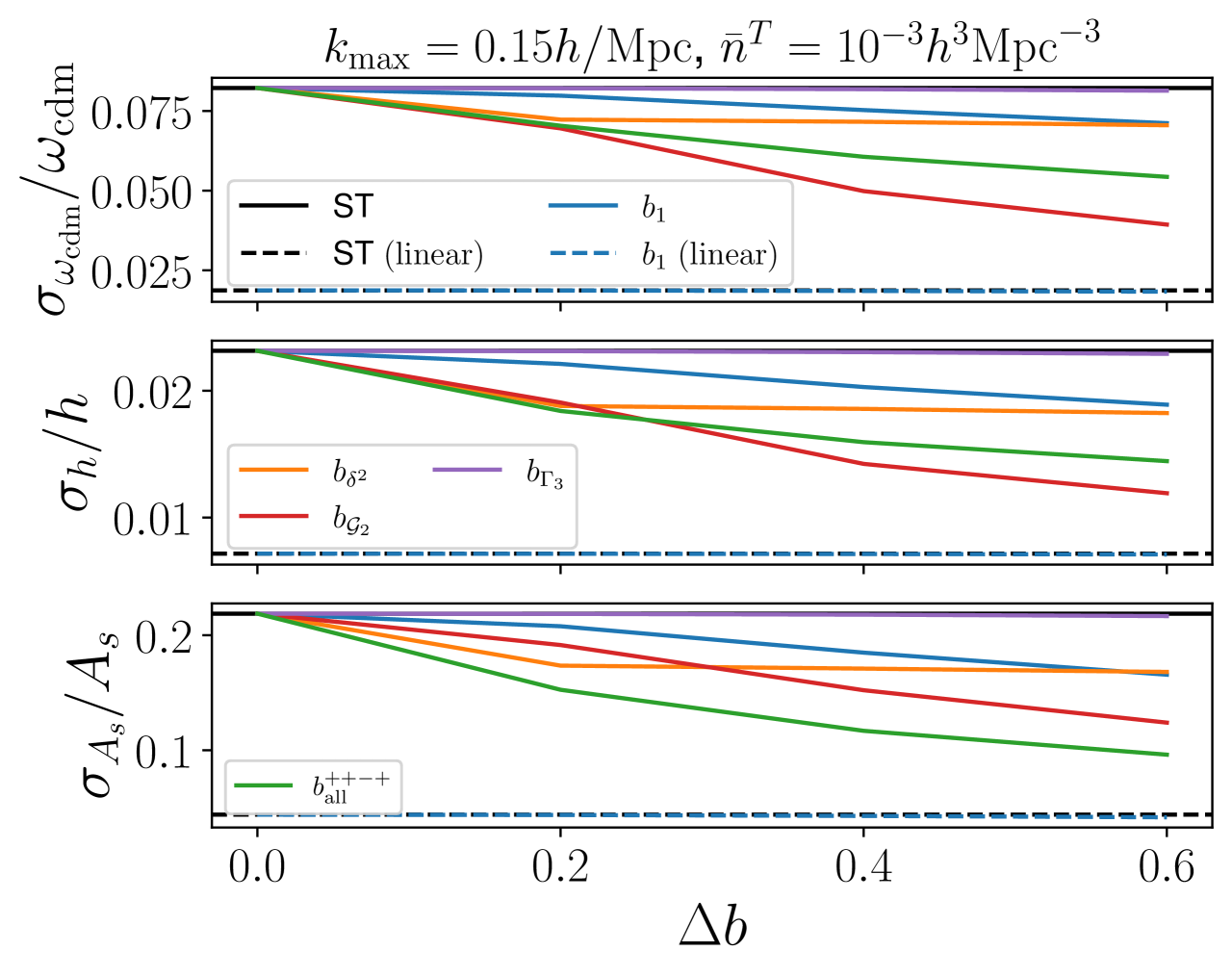
Figure 1: Relative errors in $\omega_{\rm cdm}$, $h$ and $A_{s}$ as a function of the difference in each bias parameter, $\Delta b$. The solid (dashed) black line represents the single-tracer EFT (linear) results, while the dashed blue line corresponds to a multi-tracer split in $b_{1}$ in linear theory. The $b_{\rm all}^{++-+}$ curve indicates a simultaneous split in all four bias parameters, with the $\pm$ signs denoting the sign of $b_{1}$, $b_{\delta^{2}}$, $b_{\mathcal{G}_{2}}$, $b_{\Gamma_{3}}$ for the $t_{2}$ sample, as described in Eq. (2.27). We consider $k_{\rm max}=0.15\,h/$Mpc (see Fig. 12 for $k_{\rm max}=0.05\,h/$Mpc) and assume a tracer number density $\bar{n}^{T}=10^{-3}\,h^{3}{\rm Mpc}^{-3}$.

For comparison, the dashed lines in Fig. 1 represent the results obtained using linear theory. Naturally, the error bars are smaller in that case, as fewer parameters need to be marginalized over. However, the absence of EFT corrections may lead to biased cosmological parameters, given that we are considering relatively nonlinear scales. The blue dashed line indicates a split in $b_{1}$ within linear theory, where we see a very mild dependence on $\Delta b_{1}$. As we discuss in Sec. 3.3, MT provides improved results under a linear split only when the cross-stochastic term is neglected or for very high values for $\bar{n}^{T}$. We find that a split in $\Delta b_{1}$ yields significantly better results when non-linear corrections are included, even when accounting for cross-stochasticity. This improvement is likely to happen due to extra degeneracy breaks in the non-linear operators (see Sec. 3.3), e.g. in terms proportional to $b_{1}b_{O}$.

We also show in Fig. 1 the result for a tracer split in all bias parameters simultaneously, denoted as $b_{\rm all}^{++-+}$. The four $\pm$ signs in the superscript represent the signs of $b_{1}$, $b_{\delta^{2}}$, $b_{\mathcal{G}_{2}}$, $b_{\Gamma_{3}}$ for the $t_{2}$ sample, as indicated by Eq. (2.27). Interestingly, this split does not necessarily lead to better results compared, for example, to a split in $b_{\mathcal{G}_{2}}$, particularly for $\omega_{\rm cdm}$ and $h$. This suggests that the Fisher information may be more sensitive to non-trivial parameter combinations rather than the simple variation of all bias coefficients in a single direction. In Fig. 12 of App. C, we also present results for $b_{\rm all}^{+\pm\pm\pm}$, with different sign combinations. In general, we find that splitting all four bias parameters together consistently performs better than a simple split in the linear bias $b_{1}$. From here on, we show results as a function of $b_{\rm all}^{++-+}$ (hereafter referred to simply as $b_{\rm all}$), where the sign of $b_{\mathcal{G}_{2}}$ is flipped, as a proxy of a generic tracer split. We display in Fig. 2 the monopole, quadrupole and hexadecapole spectra for the MT scenario relative to the ST case. The left panel shows the effects of a split in $b_{1}$ and the right panel illustrates the case of a split in $b_{\rm all}$, where all bias parameters are varied simultaneously by the same $\Delta b$. Notice that the monopoles are not exactly the same for $\Delta b=0$ due to the $\frac{1}{2}$ factor of difference in the number density, which enters in the stochastic part.

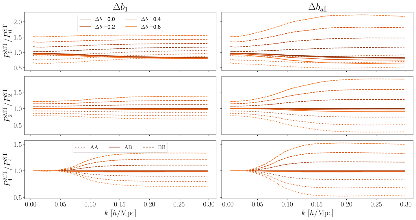
Figure 2: Monopole, quadrupole and hexadecapole normalized by the ST spectra for a bias split in $b_{1}$ (left) and $b_{\rm all}$ (right). Different colors correspond to various $\Delta b$ value. Dotted, solid and dashed lines correspond to the auto AA, cross AB and auto BB spectra, respectively.

We summarize the results in Tab. 1, where we fixed $\Delta b=0.6$. We find that a split in $b_{1}$ using linear only results in a $5\%$ improvement in $A_{s}$ with barely any gain for the other two cosmological parameters. On the other hand, considering a split in $b_{1}$ and using non-linear theory leads to improvements of $13\%$ in $\omega_{\rm cdm}$, $18\%$ in $h$ and $24\%$ in $A_{s}$. When split in the full set of bias parameters simultaneously, the improvements reach $34\%$ in $\omega_{\rm cdm}$, $38\%$ in $h$ and $56\%$ in $A_{s}$. Those values are comparable to the findings of [45, 46]. Thus, we find that selecting samples with significantly different bias parameters can considerably enhance cosmological constraints, sometimes reducing the error bars by a factor two or more.

	$b_{1}$ (linear)	$b_{1}$ (EFT)	$b_{\rm all}$ (EFT)
$\sigma_{\omega_{\rm cdm}}^{\rm MT}/\sigma_{\omega_{\rm cdm}}^{\rm ST}$	0.98	0.87	0.66
$\sigma_{h}^{\rm MT}/\sigma_{h}^{\rm ST}$	0.99	0.82	0.62
$\sigma_{A_{s}}^{\rm MT}/\sigma_{A_{s}}^{\rm ST}$	0.95	0.76	0.44

Table 1: MT improvement relative to the ST result for $\Delta b=0.6$, shown for a split in the linear bias (both linear and non-linear modeling) and a split in $b_{\rm all}$. We assume $\bar{n}^{T}=10^{-3}\,h^{3}{\rm Mpc}^{-3}$.

3.2 The bias split using the halo mass

In this section, we discuss how likely it is to find a difference $\Delta b$ in a galaxy sample, putting the results of the previous section into perspective. We anticipate that, in a vanilla scenario, it is very difficult to find a large difference in the (linear and non-linear) bias, but assembly bias can substantially enhance this difference to potentially reach $\Delta b\sim 1$. To do so, we consider a halo sample following Tinker’s mass function [81] and linear bias [82]. We restrict our analysis to halos of masses in between $10^{13}M_{\odot}/h$ and $10^{15}M_{\odot}/h$, which typically lead to larger bias values. The values of $b_{\delta^{2}}$ are determined using its functional fit from separate Universe simulations [83] for halos

$$b_{\delta^{2}}(b_{1})=0.206-1.071b_{1}+0.464b_{1}^{2}+0.004b_{1}^{3}\,.$$ (3.1)

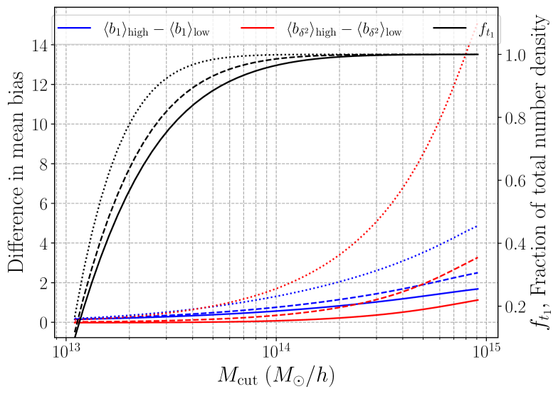
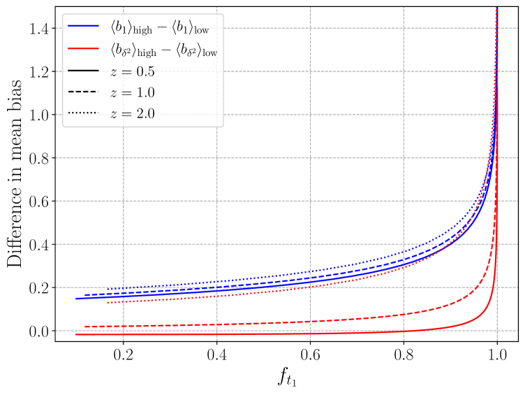
Figure 3: In the left panel, the difference in the mean values of $b_{1}$ (blue) and $b_{\delta^{2}}$ (red) between the lower and higher mass samples defined by a cut $M_{\rm cut}$. Different redshifts are represented by different line styles (solid, dashed and dotted lines). We show $f_{t_{1}}$, the density fraction of the lower mass tracer $t_{1}$ [see Eq. (3.2)], as black lines, with its values indicated on the right y-axis. In the right panel, the same differences are plotted as a function of $f_{t_{1}}$.

We consider a threshold $M_{\rm cut}$ to divide the sample into two subsets with different $b_{1}$ and $b_{\delta^{2}}$ distributions. The quantities $\langle b_{1}\rangle_{\rm low}$ and $\langle b_{1}\rangle_{\rm high}$ represent the mean value of $b_{1}$ in the lower and higher-mass subsets, respectively, where the expectation value is weighted by the Tinker’s mass function (using the values for $\Delta=200$ of [81]). Similarly, $\langle b_{\delta^{2}}\rangle_{\rm low}$ and $\langle b_{\delta^{2}}\rangle_{\rm high}$ represent the mean quadratic bias for each subset. We show the difference between the higher-mass and lower-mass biases as a function of $M_{\rm cut}$ for different redshifts (solid, dashed, dotted lines) in the left panel of Fig. 3. We also display as black lines the fraction of the tracer $t_{1}$ number density relative to the total number density

$$f_{t_{1}}=\frac{\bar{n}^{t_{1}}}{\bar{n}^{T}}\,.$$ (3.2)

We plot in the right panel of Fig. 3 the bias difference as a function of $f_{t_{1}}$. This exercise, focused on halos split by their mass, shows that it is relatively hard to obtain a large difference in $b_{1}$ and $b_{\delta^{2}}$ between the samples, unless one considers large values of $f_{t_{1}}$ or high redshift. As we discuss later in Sec. 4.2, the MT information gains relative to ST are present as long as $0.1\lesssim f_{t_{1}}\lesssim 0.9$. Although this range allows for relatively unbalanced samples and offers more freedom to find subtracers with different bias, our vanilla analysis for halos indicates that it is difficult to have large non-linear bias differences at low redshift. Finally, we comment on a possible split in $b_{\mathcal{G}_{2}}$ or $b_{\Gamma_{3}}$. Notice that a split in $b_{\mathcal{G}_{2}}$ was among the most effective for MT in Fig. 1. When we restrict ourselves to the standard local-in-matter-density (LIMD) expression for halos [84, 62]

$$b_{\mathcal{G}_{2}}(b_{1})=-\frac{2}{7}(b_{1}-1)\,,\quad\textrm{and}\quad b_{\Gamma_{3}}(b_{1})=-\frac{23}{42}(b_{1}-1)\,,$$ (3.3)

this immediately implies a factor $2/7$ and $23/42$ suppression in the difference in $b_{\mathcal{G}_{2}}$ and $b_{\Gamma_{3}}$, respectively, relative to $b_{1}$.

The above results indicate a very pessimistic scenario for finding tracers with different non-linear bias parameters. However, we should keep in mind that these findings are restricted to halos that follow either the separate Universe fits of Eq. (3.1) or the LIMD relations. In a more realistic scenario, several effects can enhance the difference between samples. First, assembly bias can be very relevant, particularly for $b_{\mathcal{G}_{2}}$; for instance, [63] has shown that $b_{\mathcal{G}_{2}}$ strongly deviates from the LIMD relation, indicating the possibility of finding very strong dependence of $b_{\mathcal{G}_{2}}$ on other properties beyond the halo mass. Finding a difference $\Delta b_{\mathcal{G}_{2}}\sim 1.0$ appears to be relatively realistic considering assembly bias (see Fig. 5 of [63]). Second, realistic galaxies samples may also strongly deviate from the relations that hold for halos [85]. A more comprehensive study on the feasibility of finding two samples with distinct nonlinear biases is beyond the scope of this work, and we leave it for a future project.

3.3 The multi-tracer information content

In this section, we investigate the MT information content. A central aspect of MT analysis is that the dataset is rearranged so that, instead of considering a single spectrum, we have

$$\frac{N_{\rm Tracers}\times(N_{\rm Tracers}+1)}{2}\,,$$ (3.4)

spectra, which includes both auto and cross-spectra between different tracers. The trade-off is that the number of biases, counter-terms, and stochastic parameters increases. While in the ST case we have $N_{\rm bias}$, $N_{\rm ct}$ and $N_{\rm stoch}$, in the MT these grow to

$$N_{\rm Tracers}\times N_{\rm bias} \quad\textrm{bias parameters}\,,$$ (3.5)

$$N_{\rm Tracers}\times N_{\rm ct} \quad\textrm{counter-terms}\,,$$ (3.6)

$$\frac{N_{\rm Tracers}\times(N_{\rm Tracers}+1)}{2}\times N_{\rm stoch} \quad\textrm{stochastic parameters}\,.$$ (3.7)

Whether the expanded data array in MT compensates for the increased number of parameters is a fundamental question in assessing its relative information gain.

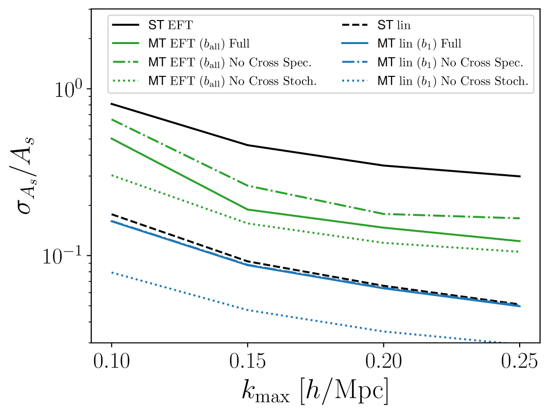
Figure 4: Relative error in $A_{s}$ as a function of the maximum mode $k_{\rm max}$ included in the analysis. The solid lines represent the full MT analysis, which includes both the cross spectra and the cross stochastic terms. When the cross-stochastic parameters are removed (dotted lines), the error bars decrease, while completely removing the cross spectra (dash-dotted lines) leads to an increase in the error bars.

We start by discussing the relevance of the cross spectra. We show in Fig. 4 the relative error in $A_{s}$ as a function of the maximum $k_{\rm max}$ mode considered in the analysis, fixing the tracer number density $\bar{n}^{T}=10^{-3}\,h^{3}{\rm Mpc}^{-3}$. Similar results apply for $\omega_{\rm cdm}$ and $h$. We compare the MT and ST case in two different scenarios: one with a linear modeling and a split in $b_{1}$ and another with a nonlinear modeling and with a split in $b_{\rm all}$. The solid lines describe the full analysis, including both the cross-spectra and the cross-stochastic terms. In contrast, the dashed-dotted lines correspond to a case where we removed the cross-spectra between the two tracers, keeping only the auto correlations in Eq. (2.18). For the EFT case, we observe that removing the cross spectra leads to a loss of information, with the result approaching the ST case. However, the gains are not completely lost when removing the cross-spectra, indicating that MT still overcomes ST even when considering the auto spectra alone. For the linear case, we notice that the MT full-analysis line closely follows the ST case. Moreover, removing the cross-spectra results in no information loss, as the two solid and dashed-dotted lines completely overlap.

Another key question in MT analysis is whether cross-stochasticity in the cross-spectra can be neglected. As discussed earlier, the linear case shown in Fig. 4 suggests that MT provides almost no improvement over ST when cross-stochasticity is included in the cross spectra [Eq. (2.9) for $i\neq j$]. For comparison, we display in dotted lines the same scenario but with the cross-stochastic contribution removed. In this case, a considerable information gain is observed. This indicates that the success of MT in linear theory seems to strongly depend on the assumption of no cross-stochasticity between the tracers. In the nonlinear case, we also observe an increase in information gain when removing the cross-stochastic parameters. However, different than the linear case, MT already shows a significant improvement over ST even when cross-stochasticity is included. This highlights a fundamental difference in the information budget of MT between linear and nonlinear theory, aligning with the findings of [45, 46].

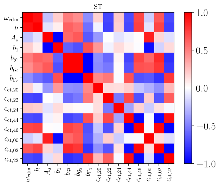
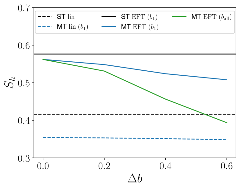
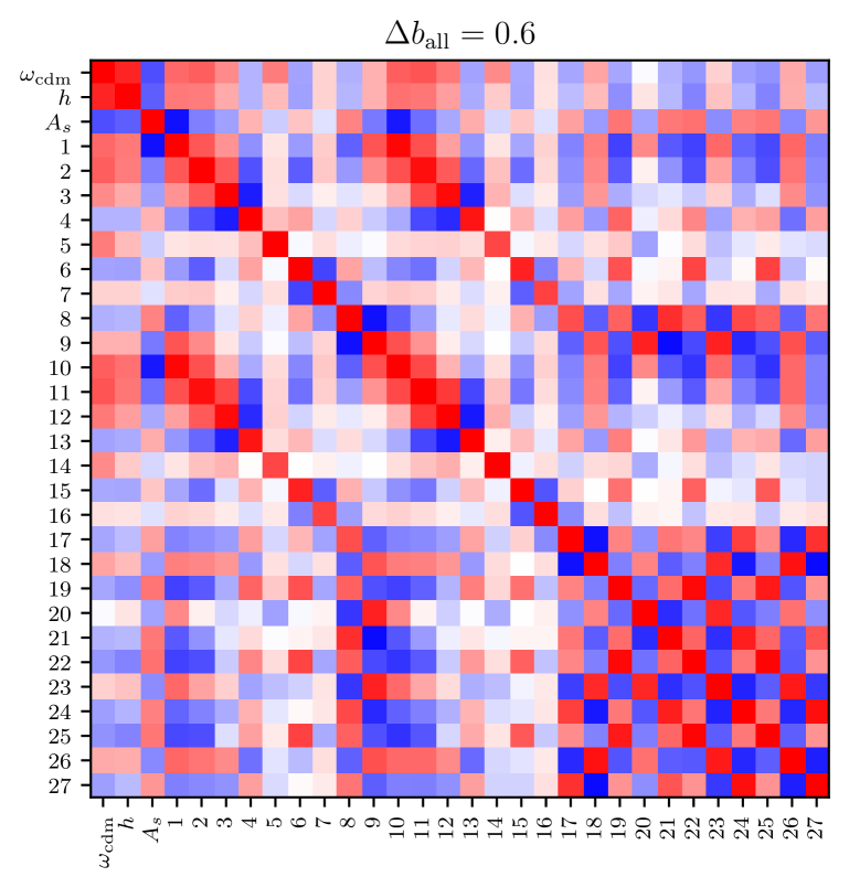
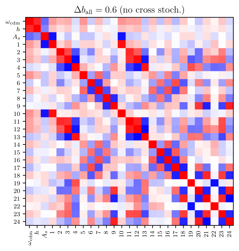
Figure 5: Correlation matrices between the parameters for the ST case (top), and MT both with (left) and without (right) the cross-stochastic operator. For the MT, we fix $\Delta b_{\rm all}=0.6$. To avoid cluttering the MT matrices with labels, we denote the bias, counter-terms, and stochastic parameters by numbers, arranged in the same order as in the ST case (i.e., AA, AB, then BB). On the top right, the parameter correlation score defined in Eq. (3.9) as a function of $\Delta b$.

We now investigate whether MT helps break degeneracies between free parameters. As pointed out in [45, 46], the MT basis can be more diagonal, meaning that part of the information gain comes from choosing a parameter basis that better separate internal degeneracies. We show in Fig. 5 the parameters (Pearson) correlation matrix

$$r_{ij}=\frac{(F^{-1})_{ij}}{\sqrt{(F^{-1})_{ii}(F^{-1})_{jj}}}\,,$$ (3.8)

between the parameters $i$ and $j$. We present results for the ST case (top left) and for MT scenarios with a split in $b_{\rm all}$, both including (bottom left) and excluding the cross stochastic term (bottom right). Overall, we observe that cross correlations between cosmological and other parameters tend to be smaller in the MT case, particularly when cross-stochasticity is removed.

To quantify the degeneracy breaking, we define the cross correlation score for the parameter $\theta_{i}$ as

$$S_{\theta_{i}}^{2}=\frac{1}{N-1}\sum_{\begin{subarray}{c}j=1\\ j\neq i\end{subarray}}^{N}r_{ij}^{2}\,,$$ (3.9)

which represents the average squared value of the non-diagonal elements, with $N$ being the total number of parameters. Lower values indicate a more orthogonal basis for the parameter $i$. We display this score for $h$ in the top right panel of Fig. 5, showing results for three cases: linear modeling with a split in $b_{1}$, nonlinear modeling with a split in $b_{1}$ and nonlinear modeling with a split in $b_{\rm all}$. For the linear case, we find a small improvement of MT when breaking degeneracies compared to the ST scenario, but we could only find a very mild dependence with $\Delta b_{1}$. In the non-linear modeling, MT exhibits a clear degeneracy break compared to ST, but we also find strong dependence in $\Delta b$. This indicates that a large difference in the bias leads to a more orthogonal basis for the cosmological parameters. The dependence on $\Delta b_{\rm all}$ is even stronger than on $\Delta b_{1}$, indicating that using all bias parameters together may lead to greater degeneracy breaking, particularly coming from the non-linear terms.

4 More tracers and the shot-noise dependence

In this section we extend the results of the former section to consider more than two tracers in Sec. 4.1 and different tracer number densities in Sec. 4.2.

4.1 More than two tracers

A natural question is why not to further consider splittings into more $N_{\rm Tracers}$ instead of just two tracers. There is, however, a trade-off between splitting into more tracers and the enhancement of the shot-noise contribution which eventually overtakes the total signal, since $\bar{n}^{t_{i}}=\bar{n}^{T}/N_{\rm Tracers}$, when considering all the subtracers with the same number density. In this work, we explore for the first time the possibility of a split into more than two tracers when including non-linear parameters in the galaxy clustering modeling.

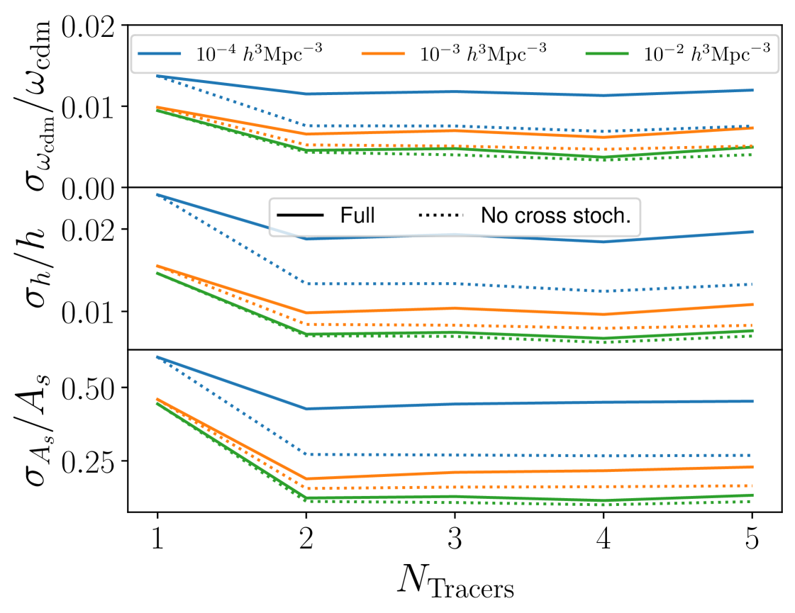
Figure 6: Relative errors in $\omega_{\rm cdm}$, $h$ and $A_{s}$ as a function of the number of tracers $N_{\rm Tracers}$ and for different $\bar{n}^{T}$ values. We fix $b_{\rm all}=0.6$. For the solid lines, we include the cross-stochastic terms and we exclude them for the dashed lines.

We display as solid lines in Fig. 6 the evolution of the Fisher estimated error in $\omega_{\rm cdm}$, $h$ and $A_{s}$ as a function of the number of tracers, having $b_{\rm all}=0.6$ fixed. For the tracer split with more tracers, we generalize Eq. (2.27) using evenly spaced MT bias parameters

$$b_{\mathcal{O}}^{t_{i}}=b_{\mathcal{O}}^{\rm ST}\pm\Delta b\left(\frac{i-1}{N_{\rm Tracers}-1}-\frac{1}{2}\right)\,,$$ (4.1)

with $i$ ranging from $1$ to $N_{\rm Tracers}$. We show results for three different values of $\bar{n}^{T}=\{10^{-4},10^{-3},10^{-2}\}\,h^{3}{\rm Mpc}^{-3}$. We find that, for all values of $\bar{n}^{T}$, $N_{\rm Tracers}=2$ seems to be the optimal number of tracers, at least when considering only the power spectrum in the analysis. Increasing the number of tracers barely improves the result, making it even slightly worst when $N_{\rm Tracers}=5$. Finally, we also include the case of more tracers without the cross-stochastic contribution as dotted lines in Fig. 6. Interestingly, $N_{\rm Tracers}=2$ also appears to be the optimal case when neglecting cross-stochasticity.

4.2 The dependence on the total and relative number density

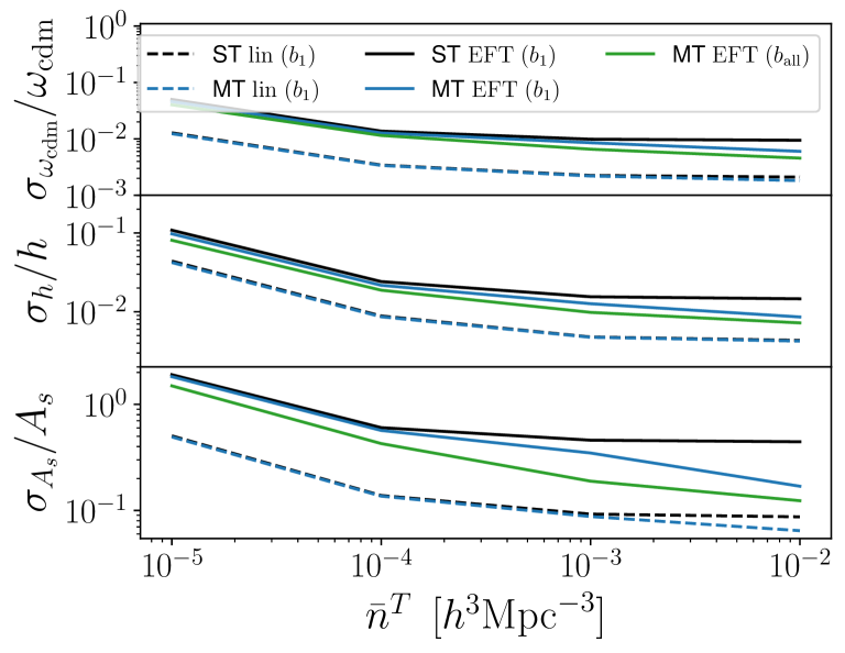
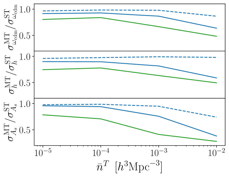
Figure 7: In the left panel, the relative error in the cosmological parameters as a function of the total number density $\bar{n}^{T}$. Dashed lines correspond to linear theory while solid lines represent the EFT non-linear theory. For the EFT MT analysis, we consider splits in $b_{1}$ and $b_{\rm all}$. In the right panel, the same results normalized by the corresponding ST scenarios. We fix $b_{1}=0.6$ or $b_{\rm all}=0.6$.

As mentioned, the trace split in MT analysis reduce the relative number density of each subsample increasing their relative shot-noise. Therefore, the MT gains are directly connected to the total tracer density of the initial sample. In this section we investigate the dependence of the MT gain on the total sample density as well as the relative number density of the subsamples.

We display in the left panel of Fig. 7 the relative error as a function of the total number density. We normalize by the ST error in the right panel. The dashed lines represent the linear theory, in which we see that MT barely outperforms ST. As we discussed in Sec. 3.3, the success of MT in linear theory strongly depends on neglecting the cross-stochasticity. The solid lines represent the Fisher errors when including non-linear bias and counter-terms. For the MT non-linear case, we consider both a split in $b_{1}$ and in $b_{\rm all}$. We can observe that, for the linear case, the main improvement from MT is in $A_{s}$ and starting at $\bar{n}^{T}>10^{-3}\,h^{3}{\rm Mpc}^{-3}$. When considering the non-linear case, the MT errors are substantially smaller for a broader range of $\bar{n}^{T}$ and also in $\omega_{\rm cdm}$ and $h$. The split in all the bias parameters together, $b_{\rm all}$, always lead to smaller error bars compared to the usual $b_{1}$ split. The well known saturation of the Fisher information with $\bar{n}^{T}$ for the ST case happens at both linear and non-linear scenarios. This is not the case for MT both linear and non-linear.

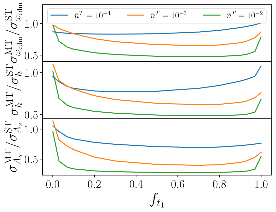
Figure 8: Error in the cosmological parameters normalized by the ST error as a function of the fraction of the total number density in tracer $t_{1}$ for a non-balanced split, defined as $f_{t_{1}}=\bar{n}^{t_{1}}/\bar{n}^{T}$. Different colors correspond to different values of $\bar{n}^{T}$, in units of $h^{3}/$Mpc³. As before, we fix $b_{\rm all}=0.6$.

When performing a MT split, we also have the freedom to chose the number densities of the final tracers with respect to the initial sample. In [45, 46] we have only consider a balanced split, in which each subtracer has the same number density. Here we extend this analysis by studying the MT performance as a function of the tracer $t_{1}$ fraction, defined in Eq. (3.2). In this work, we keep the MT relative bias difference $\Delta b$ constant with $f_{t_{1}}$. However, it is important to note that in realistic scenarios where the two samples are split based on a tracer feature, $\Delta b$ is expected to change with $f_{t_{1}}$ (see Sec. 3.2). Since this dependence heavily depends on the sample considered, we assume for simplicity a constant bias difference. We display in Fig. 8 the error as a function of $f_{t_{1}}$ for different values of $\bar{n}^{T}$ normalized by the ST error. Note that the case $f_{t_{1}}\to 0$ or $f_{t_{1}}\to 1$, for which the full density is in one of the samples, does not reproduce the ST case for the same fiducial bias parameters Eq. (2.26), but rather corresponds to a different set of bias parameters shifted by $\Delta b$. We see a typical $U$-shape curve with a relatively flat region for $0.1\lesssim f_{t_{1}}\lesssim 0.9$, which is especially present as we increase $\bar{n}^{T}$. It indicates that, despite the optimal value normally being close to the balanced case $f_{t_{1}}=0.5$, the MT improvements are also present with some unbalancing between both tracer densities. Notice that, in general, it is easier to find subsamples with distinct bias parameters if allowing for their number densities to not be exactly the same. One can, for instance, find the 10 or $20\%$ galaxies with lower or higher values for $b_{\mathcal{G}_{2}}$ and already benefit from the MT information gains.

5 FoG and different $k_{\rm max}$

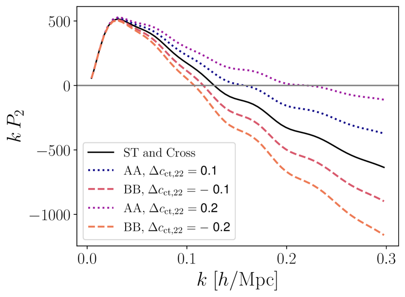
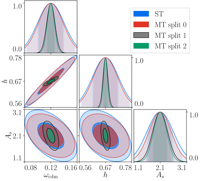
Figure 9: In the left panel, the quadrupole for the ST case (black), for the blue sample A and for the red sample B. Notice that the cross spectra coincides with the ST line for a tracer split in $c^{\rm ST}_{{\rm ct},22}$. In the right panel, the Fisher contours for different $k_{\rm max}$ cuts in the MT case compared to the ST case (see Tab. 2).

In this section, we elaborate on how MT can be useful to distinguish between samples with different Fingers-of-God perturbative regimes, such that we could potentially use different $k_{\rm max}$ for different subsamples to maximize the information extracted. For instance, if one performs a color split, red samples live in more virialized structures and therefore have larger peculiar velocities [87, 88, 89]. The enhancement of the FoG was analysed in the MT context in [46] (see Fig. 1 therein), where it was shown that the MT split can enhance the FoG effect for one of the samples. Improving the FoG treatment can also be done via a rearrangement of the multipole expansion [90, 91, 92, 93] or by sub-sample selection [94]. In this work, we consider the possibility of having different scale cuts $k_{\rm max}$ for the two MT subsamples, such that we do not throw away any information, but treat the perturbative reach differently for the subsamples. The fact that the bluer subsample suffers less FoG suppression can allow for a sensible increase in its relative $k_{\rm max}$ which leads to information gain.

The FoG suppression of the quadrupole can be emulated in the bias expansion as a sharp drop in the quadrupole via a large (negative) $c_{{\rm ct},22}$ counter-term. To make this effect more pronounced, we adopt in this part the same fiducial parameters as Eq. (2.26) but also taking $c^{\rm ST}_{{\rm ct},22}=-0.3$. We perform a MT split in $c_{{\rm ct},22}$ with the idea of mimicking a color split: the red sample is characterized by a more negative $c_{{\rm ct},22}$ and larger FoG suppression, while the blue sample has a more positive $c_{{\rm ct},22}$ value and less FoG suppression on the quadrupole. We illustrate the split in the left panel of Fig. 9.

Motivated by [94], which treats the zero crossing of the quadrupole a proxy for the perturbative failing of the FoG treatment, we adopt different values of $k_{\rm max}$ for the different samples. We shown in Tab. 2 the zero-crossing value for the different samples. We notice that a relatively small shift $\Delta c_{{\rm ct},22}=0.2$ allows for an increase in $k_{\rm max}$ from 0.124$h/$Mpc to 0.208$h/$Mpc. We are assuming that the perturbative scale for dark matter $k_{\rm NL}$ and the higher-derivative expansion scale $1/R_{\rm Halo}$, associated with the Lagrangian halo scale, are smaller than the scales considered here, $k_{\rm NL}>k_{\rm max}$ and $1/R_{\rm Halo}>k_{\rm max}$. We display in the right panel of Fig. 9 the expected error bars for the different $k_{\rm max}$ considered in Tab. 2. We find a notable improvement compared to the ST case due to the tracer split and the higher $k_{\rm max}$ of the bluer sample. This result points out to MT as a natural way to improve the perturbative treatment for FoG.

	$k_{\rm max}^{AA}$	$k_{\rm max}^{ST/AB}$	$k_{\rm max}^{BB}$
ST	-	0.124	-
MT split 0 ($|\Delta c_{{\rm ct},22}|=0.0$)	0.124	0.124	0.124
MT split 1 ($|\Delta c_{{\rm ct},22}|=0.1$)	0.157	0.124	0.114
MT split 2 ($|\Delta c_{{\rm ct},22}|=0.2$)	0.208	0.124	0.105

Table 2: Different $k_{\rm max}$ values (in units of $h/$Mpc) used for the auto, cross and single tracer spectra based on the zero-crossing of the quadrupole.

6 Forecasts

In this section, we forecast the MT scenario for different galaxy survey configurations. For simplicity, we compress the survey data into a single redshift bin. While this is a simplified scenario, it can serve as a good guidance to estimate the MT improvements relative to ST. We use for the effective volume [95]

$$V_{\text{eff}}\approx\sum_{i}V(z_{i})\left[\frac{b_{1}^{2}(z_{i})P_{\rm L}(z_{i})/\overline{n}(z_{i})}{1+b_{1}^{2}(z_{i})P_{\rm L}(z_{i})/\overline{n}(z_{i})}\right]^{2}_{k=0.10\,\frac{h}{\text{Mpc}}}\,,$$ (6.1)

summing over multiple redshift bins $z_{i}$ and anchoring the power spectra at $k=0.1\,h/$Mpc. In addition, we compute the effective number density $\overline{n}_{\text{eff}}$ and the effective redshift $z_{\text{eff}}$ by averaging $\overline{n}(z_{i})$ and $z_{i}$ weighted by the number of tracers $N_{i}=\overline{n}(z_{i})V(z_{i})$ in the corresponding redshift bin. For the linear bias, we use $b_{1}^{\rm eff}(z_{\rm eff})=0.9+0.4z_{\rm eff}$, which has been used in other works [8, 95, 96] and is based on [97]. For simplicity, we fix the other non-linear bias parameters to Eq. (2.26). We summarize in Tab. 3 the surveys and their specifications used in this section.

experiment	$z_{\text{eff}}$	$b_{1,\text{eff}}$	$\overline{n}_{\text{eff}}$ (in $10^{-3}\frac{h^{3}}{\text{Mpc}^{3}}$)	$V_{\rm eff}$ (in $\frac{\text{Gpc}^{3}}{h^{3}}$)	reference
BOSS	$0.57$	$1.13$	$0.88$	$2.29$	[98]
PFS	$1.50$	$1.50$	$0.50$	$2.98$	[96]
Roman	$1.37$	$1.45$	$2.56$	$8.50$	[99]
DESI	$1.02$	$1.31$	$0.58$	$12.2$	[4]
Euclid	$0.94$	$1.27$	$2.06$	$24.5$	[100, 95]
MegaMapper	$2.45$	$1.88$	$1.69$	$52.8$	[101, 102]

Table 3: Summary of the surveys parameter values considered in this work, along with the references used to obtain their specifications.

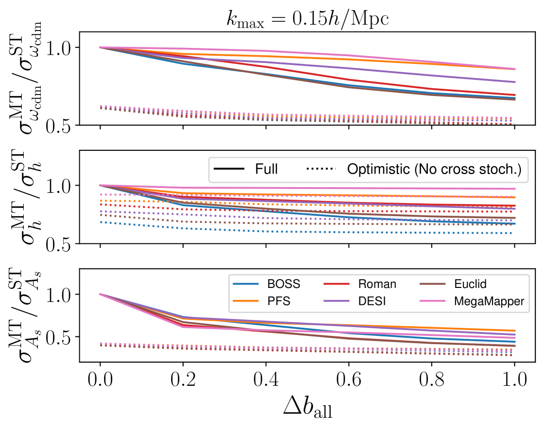
Figure 10: MT error in the cosmological parameters relative to ST as a function of the difference $\Delta b_{\rm all}$ in all the bias simultaneously. Different colors represent different surveys. The dotted lines represent the analysis without cross-stochasticity.

The forecast results are presented in Fig. 10 as a function of $\Delta b_{\rm all}$. The solid lines represent the most conservative scenario in which we include all the terms, while the dashed lines represent the most optimistic case in which the cross-stochastic component is neglected. We find a factor 2 improvement in $A_{s}$ across all surveys. We also find significant improvement in $h$ and $\omega_{\rm cdm}$, but somewhat smaller for PFS and MegaMapper, which we checked to be due the high $z$ considered for those surveys. The non-linear corrections are very small at high redshift at $k=0.15\,h/$Mpc, and typically one can reach higher values of $k_{\rm max}$ at high $z$. A more comprehensive study which considers the different redshift bins of each survey and models their respective $k_{\rm max}$ values as a function of redshift, is left for future work. Finally, when the cross-stochastic component is neglected, we find even stronger MT constraints, highlighting the importance of adding simulation-based priors on these parameters.

7 Conclusions

In this article, we have extended the results of [45, 46] carrying a systematic study of MT when considering the non-linear modeling of galaxy clustering. We employ a series of Fisher studies to investigate different scenarios, including various survey configurations. Within the large-scale bias expansion, any tracer split based on a specific sample feature can be mapped into a direct split in the bias parameters. Accordingly, we display our results as a function of the difference $\Delta b$ in the bias coefficients and show that the MT Fisher information reproduces the ST scenario when taking $\Delta b\to 0$. Further, we discuss how likely it is to identify two halo samples with differing non-linear bias parameters. While such differences are hard to find in a vanilla scenario, the presence of assembly bias and the use of realistic galaxy samples can lead to $\Delta b_{\mathcal{G}_{2}}\sim 1$ [63]. This paper paves the way toward identifying a MT bias split that does not necessarily rely on finding two samples with very different linear bias coefficients.

Next, we study the importance of cross-stochasticity for MT. We show that neglecting this term is vital for MT within linear theory, while this appears not to be the case when considering the non-linear bias modeling. Furthermore, we show for the first time, using non-linear modeling, that a split into two tracers seems to maximize the information gain, at least when restricted to a power spectra analysis. We have also found that, when considering the non-linear operators, the MT gains are present at very realistic number density values, in contrast with the findings on linear theory that demands very high tracer densities. We addressed the question of what are the optimal number densities between the two subtracers, finding substantial gains even when considering a very unbalanced split, i.e. when one the tracers is more dense than the other. This result makes the task of finding two tracers with two different set of biases simpler, since we can limit the MT searches to find a small in-homogeneous subsample. Finally, in Sec. 5 we consider the possibility of using different values of $k_{\rm max}$ for the subtracers depending on the strength of the FoG effect for each. We show how this approach can substantially enhance the information extracted from the bluer sample.

We plan to apply in the short future the MT pipeline to (e)BOSS and DESI data. It would also be interesting to extend the PNG analysis of [25] to non-linear scales and investigate the information content of the MT non-linear bispectrum. Moreover, when splitting into tracers, the running of the bias parameters as a function of the cutoff $\Lambda$ also changes [65]. It would be interesting to investigate the running of the MT bias parameters in the context of the bias renormalization group.

Appendix A Stability of Fisher derivatives

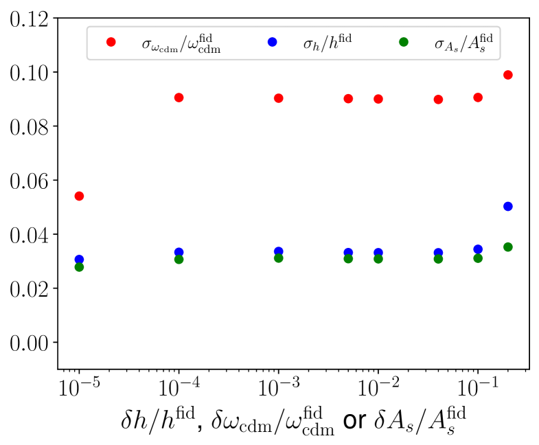
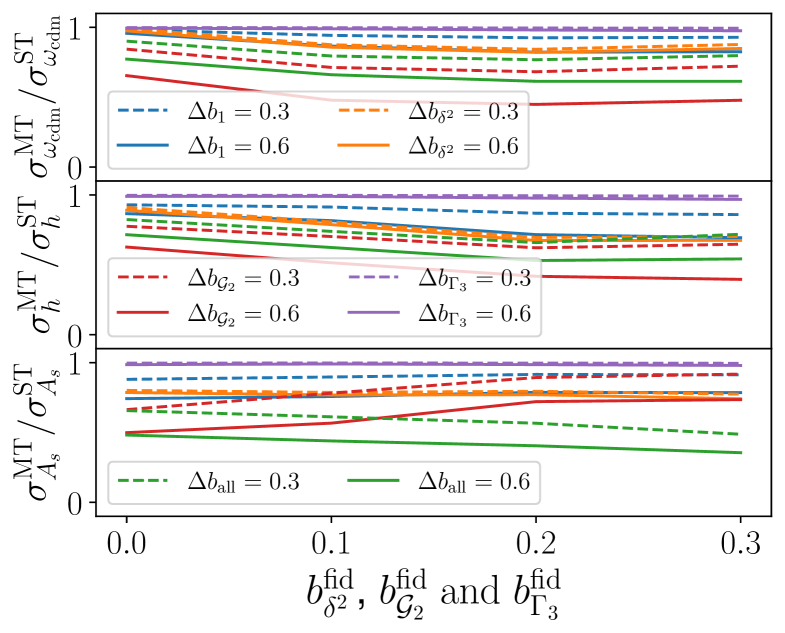
Figure 11: In the left panel, the relative error $\sigma_{h}/h^{\rm fid}$, $\sigma_{\omega_{\rm cdm}}/\omega_{\rm cdm}^{\rm fid}$ and $\sigma_{A_{s}}/A_{s}^{\rm fid}$ as a function of the relative step size $\delta h$, $\delta\omega_{\rm cdm}$ and $\delta A_{s}$ used in the (second-order) finite difference method. A small step size is consistent with noise while a large step size leads to the breakdown of the finite difference method. We adopt $\delta h/h^{\rm fid}=\delta\omega_{\rm cdm}/\omega_{\rm cdm}^{\rm fid}=\delta A_{s}/A_{s}^{\rm fid}=0.04$, where the errors remain relatively stable. In the right panel, the ratio between MT and ST error bars as a function of the fiducial bias parameters chosen in Eq. (2.26). For the MT results, we consider $\Delta b=0.3$ (dashed) and $\Delta b=0.6$ (solid) splits.

The derivatives $\partial_{\theta_{a}}P^{t_{i}t_{j}}(k_{\alpha})$ in the Fisher analysis of Eq. (2.18) can be computed analytically with respect to the bias and stochastic parameters but have to be computed numerically for $h$, $\omega_{\rm cdm}$ and $A_{s}$. To improve the stability of the numerical derivatives, we use a second-order finite difference method and compute the log-derivative $P^{t_{i}t_{j}}(k_{\alpha})\partial_{\theta_{a}}\ln P^{t_{i}t_{j}}(k_{\alpha})$. We show in the left panel of Fig. 11 the stability of the Fisher-extracted relative parameters errors $\sigma_{h}$, $\sigma_{\omega_{\rm cdm}}$ and $\sigma_{A_{s}}$ as a function of the step sizes $\delta h$, $\delta\omega_{\rm cdm}$ and $\delta A_{s}$ used for the finite difference evaluation. We observe that choosing a step size that is too small results in numerical noise, while large step sizes lead to the breakdown of the finite difference method. Intermediate values lead to relatively stable results. Based on this, we adopt the relative step size $\delta h/h^{\rm fid}=\delta\omega_{\rm cdm}/\omega_{\rm cdm}^{\rm fid}=\delta A_{s}/A_{s}^{\rm fid}=0.04$, normalized by their fiducial Planck 18 values.

Appendix B Dependence on the fiducial values

In this section, we discuss how our results depend on the fiducial values chosen for the bias parameters in Eq. (2.26). The right panel of Fig. 11 shows the ratio between the MT and ST error bars as a function of the fiducial values for $b_{1}$, $b_{\delta^{2}}$, and $b_{\mathcal{G}_{2}}$. In this analysis, we make all the fiducial bias parameters change together. For the MT results, we considered splits of $\Delta b=0.3$ (dashed) and $\Delta b=0.6$ (solid). We observe fluctuations of approximately $20\%$ in the curves, yet the overall qualitative results remain unchanged.

Appendix C Extra plots for $b_{\rm all}^{+\pm\pm\pm}$ and different $k_{\rm max}$

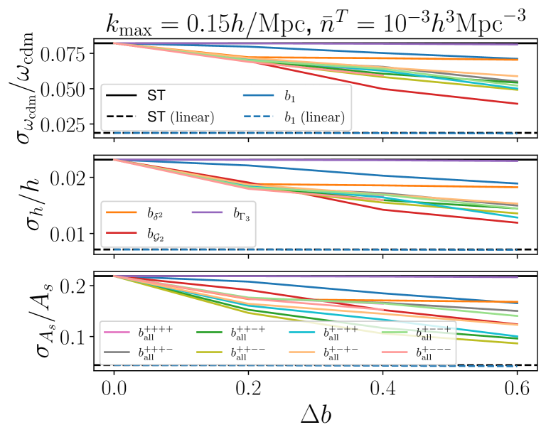
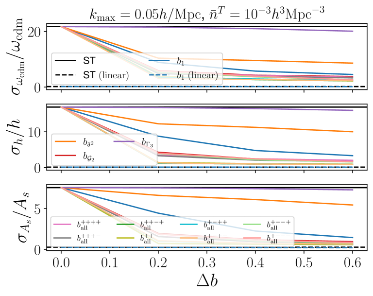
Figure 12: Same as Fig. 1, but in the left panel we include all combinations of $b_{\rm all}^{\pm\pm\pm\pm}$. The $b_{\rm all}$ lines correspond to a simultaneous split in all four bias parameters, with the $\pm$ sign indicating the sign of $b_{1}$, $b_{\delta^{2}}$, $b_{\mathcal{G}_{2}}$, and $b_{\Gamma_{3}}$ for the $t_{2}$ sample, as defined in Eq. (2.27). In the right panel, we set $k_{\rm max}=0.05h/$Mpc.

In this Appendix, we include complementary plots that were not added to the main part of the paper. In Fig. 12, the left panel displays all possible combinations of $b_{\rm all}^{+\pm\pm\pm}$; although we observe some relative differences between them, no qualitative change occurs. In the right panel, we present the same plot as in Fig. 1, but with $k_{\rm max}=0.05\,h/$Mpc. The error bars are, as expected, larger, but we find that a split in $b_{1}$ becomes relatively more important than a split in $b_{\delta^{2}}$.

References

- [1] BOSS collaboration, S. Alam et al., The clustering of galaxies in the completed SDSS-III Baryon Oscillation Spectroscopic Survey: cosmological analysis of the DR12 galaxy sample, Mon. Not. Roy. Astron. Soc. 470 (2017) 2617–2652, [1607.03155].
- [2] The Dark Energy Survey Collaboration, The Dark Energy Survey, ArXiv Astrophysics e-prints (Oct., 2005) , [astro-ph/0510346].
- [3] eBOSS collaboration, R. Ahumada et al., The 16th Data Release of the Sloan Digital Sky Surveys: First Release from the APOGEE-2 Southern Survey and Full Release of eBOSS Spectra, Astrophys. J. Suppl. 249 (2020) 3, [1912.02905].
- [4] DESI collaboration, A. Aghamousa et al., The DESI Experiment Part I: Science,Targeting, and Survey Design, 1611.00036.
- [5] Euclid Theory Working Group collaboration, L. Amendola et al., Cosmology and fundamental physics with the Euclid satellite, Living Rev. Rel. 16 (2013) 6, [1206.1225].
- [6] LSST collaboration, Z. Ivezic, J. A. Tyson, R. Allsman, J. Andrew and R. Angel, LSST: from Science Drivers to Reference Design and Anticipated Data Products, 0805.2366.
- [7] SPHEREx collaboration, O. Doré et al., Cosmology with the SPHEREX All-Sky Spectral Survey, 1412.4872.
- [8] PFS Team collaboration, R. Ellis et al., Extragalactic science, cosmology, and Galactic archaeology with the Subaru Prime Focus Spectrograph, Publ. Astron. Soc. Jap. 66 (2014) R1, [1206.0737].
- [9] G. Valogiannis, S. Yuan and C. Dvorkin, Precise cosmological constraints from BOSS galaxy clustering with a simulation-based emulator of the wavelet scattering transform, Phys. Rev. D 109 (2024) 103503, [2310.16116].
- [10] M. Eickenberg et al., Wavelet Moments for Cosmological Parameter Estimation, 2204.07646.
- [11] H. Rubira and R. Voivodic, The Effective Field Theory and Perturbative Analysis for Log-Density Fields, JCAP 03 (2021) 070, [2011.12280].
- [12] O. H. E. Philcox, E. Massara and D. N. Spergel, What does the marked power spectrum measure? Insights from perturbation theory, Phys. Rev. D 102 (2020) 043516, [2006.10055].
- [13] M. C. Neyrinck, I. Szapudi and A. S. Szalay, Rejuvenating the matter power spectrum: restoring information with a logarithmic density mapping, Astrophys. J. Lett. 698 (2009) L90–L93, [0903.4693].
- [14] M. Biagetti, J. Calles, L. Castiblanco, A. Cole and J. Noreña, Fisher forecasts for primordial non-Gaussianity from persistent homology, JCAP 10 (2022) 002, [2203.08262].
- [15] A. Banerjee and T. Abel, Nearest neighbour distributions: New statistical measures for cosmological clustering, Mon. Not. Roy. Astron. Soc. 500 (2020) 5479–5499, [2007.13342].
- [16] U. Seljak, Bias, redshift space distortions and primordial nongaussianity of nonlinear transformations: application to Lyman alpha forest, JCAP 03 (2012) 004, [1201.0594].
- [17] N.-M. Nguyen, F. Schmidt, B. Tucci, M. Reinecke and A. Kostić, How much information can be extracted from galaxy clustering at the field level?, 2403.03220.
- [18] U. Seljak, Extracting primordial non-gaussianity without cosmic variance, Phys. Rev. Lett. 102 (2009) 021302, [0807.1770].
- [19] P. McDonald and U. Seljak, How to measure redshift-space distortions without sample variance, JCAP 10 (2009) 007, [0810.0323].
- [20] L. R. Abramo and K. E. Leonard, Why multi-tracer surveys beat cosmic variance, Mon. Not. Roy. Astron. Soc. 432 (2013) 318, [1302.5444].
- [21] L. R. Abramo, L. F. Secco and A. Loureiro, Fourier analysis of multitracer cosmological surveys, Mon. Not. Roy. Astron. Soc. 455 (2016) 3871–3889, [1505.04106].
- [22] L. R. Abramo, J. a. V. Dinarte Ferri, I. L. Tashiro and A. Loureiro, Fisher matrix for the angular power spectrum of multi-tracer galaxy surveys, JCAP 08 (2022) 073, [2204.05057].
- [23] M. LoVerde, Neutrino mass without cosmic variance, Phys. Rev. D 93 (2016) 103526, [1602.08108].
- [24] N. Hamaus, U. Seljak and V. Desjacques, Optimal Weighting in Galaxy Surveys: Application to Redshift-Space Distortions, Phys. Rev. D 86 (2012) 103513, [1207.1102].
- [25] A. Barreira and E. Krause, Towards optimal and robust f_nl constraints with multi-tracer analyses, JCAP 10 (2023) 044, [2302.09066].
- [26] D. Karagiannis, R. Maartens, J. Fonseca, S. Camera and C. Clarkson, Multi-tracer power spectra and bispectra: formalism, JCAP 03 (2024) 034, [2305.04028].
- [27] C. Blake et al., Galaxy And Mass Assembly (GAMA): improved cosmic growth measurements using multiple tracers of large-scale structure, Mon. Not. Roy. Astron. Soc. 436 (2013) 3089, [1309.5556].
- [28] A. J. Ross et al., The Clustering of Galaxies in the SDSS-III DR10 Baryon Oscillation Spectroscopic Survey: No Detectable Colour Dependence of Distance Scale or Growth Rate Measurements, Mon. Not. Roy. Astron. Soc. 437 (2014) 1109–1126, [1310.1106].
- [29] F. Beutler, C. Blake, J. Koda, F. Marin, H.-J. Seo, A. J. Cuesta et al., The BOSS–WiggleZ overlap region – I. Baryon acoustic oscillations, Mon. Not. Roy. Astron. Soc. 455 (2016) 3230–3248, [1506.03900].
- [30] F. A. Marín, F. Beutler, C. Blake, J. Koda, E. Kazin and D. P. Schneider, The BOSS–WiggleZ overlap region – II. Dependence of cosmic growth on galaxy type, Mon. Not. Roy. Astron. Soc. 455 (2016) 4046–4056, [1506.03901].
- [31] P. Zhang and Y. Cai, BOSS full-shape analysis from the EFTofLSS with exact time dependence, JCAP 01 (2022) 031, [2111.05739].
- [32] J. M. Sullivan, T. Prijon and U. Seljak, Learning to concentrate: multi-tracer forecasts on local primordial non-Gaussianity with machine-learned bias, JCAP 08 (2023) 004, [2303.08901].
- [33] eBOSS collaboration, Y. Wang et al., The clustering of the SDSS-IV extended Baryon Oscillation Spectroscopic Survey DR16 luminous red galaxy and emission line galaxy samples: cosmic distance and structure growth measurements using multiple tracers in configuration space, Mon. Not. Roy. Astron. Soc. 498 (2020) 3470–3483, [2007.09010].
- [34] eBOSS collaboration, G.-B. Zhao et al., The completed SDSS-IV extended Baryon Oscillation Spectroscopic Survey: a multitracer analysis in Fourier space for measuring the cosmic structure growth and expansion rate, Mon. Not. Roy. Astron. Soc. 504 (2021) 33–52, [2007.09011].
- [35] eBOSS collaboration, C. Zhao et al., The completed SDSS-IV extended Baryon Oscillation Spectroscopic Survey: cosmological implications from multitracer BAO analysis with galaxies and voids, Mon. Not. Roy. Astron. Soc. 511 (2022) 5492–5524, [2110.03824].
- [36] N. E. Chisari, C. Dvorkin, F. Schmidt and D. Spergel, Multitracing Anisotropic Non-Gaussianity with Galaxy Shapes, Phys. Rev. D 94 (2016) 123507, [1607.05232].
- [37] F. Montano and S. Camera, Detecting relativistic Doppler by multi-tracing a single galaxy population, Phys. Dark Univ. 46 (2024) 101634, [2407.06284].
- [38] K. Tanidis and S. Camera, Developing a unified pipeline for large-scale structure data analysis with angular power spectra – III. Implementing the multitracer technique to constrain neutrino masses, Mon. Not. Roy. Astron. Soc. 502 (2021) 2952–2960, [2009.05584].
- [39] Z. Gomes, S. Camera, M. J. Jarvis, C. Hale and J. Fonseca, Non-Gaussianity constraints using future radio continuum surveys and the multitracer technique, Mon. Not. Roy. Astron. Soc. 492 (2020) 1513–1522, [1912.08362].
- [40] L. D. Ferramacho, M. G. Santos, M. J. Jarvis and S. Camera, Radio galaxy populations and the multitracer technique: pushing the limits on primordial non-Gaussianity, Mon. Not. Roy. Astron. Soc. 442 (2014) 2511–2518, [1402.2290].
- [41] A. Witzemann, D. Alonso, J. Fonseca and M. G. Santos, Simulated multitracer analyses with H i intensity mapping, Mon. Not. Roy. Astron. Soc. 485 (2019) 5519–5531, [1808.03093].
- [42] L. R. Abramo, J. a. V. D. Ferri and I. L. Tashiro, Fisher matrix for multiple tracers: the information in the cross-spectra, JCAP 04 (2022) 013, [2112.01812].
- [43] R. Boschetti, L. R. Abramo and L. Amendola, Fisher matrix for multiple tracers: all you can learn from large-scale structure without assuming a model, JCAP 11 (2020) 054, [2005.02465].
- [44] C. Heinrich, O. Dore and E. Krause, Measuring fNL with the SPHEREx multitracer redshift space bispectrum, Phys. Rev. D 109 (2024) 123511, [2311.13082].
- [45] T. Mergulhão, H. Rubira, R. Voivodic and L. R. Abramo, The effective field theory of large-scale structure and multi-tracer, JCAP 04 (2022) 021, [2108.11363].
- [46] T. Mergulhão, H. Rubira and R. Voivodic, The effective field theory of large-scale structure and multi-tracer II: redshift space and realistic tracers, JCAP 01 (2024) 008, [2306.05474].
- [47] R. Zhao et al., A multitracer analysis for the eBOSS galaxy sample based on the effective field theory of large-scale structure, Mon. Not. Roy. Astron. Soc. 532 (2024) 783–804, [2308.06206].
- [48] H. Ebina and M. White, Cosmology before noon with multiple galaxy populations, JCAP 06 (2024) 052, [2401.13166].
- [49] D. Baumann, A. Nicolis, L. Senatore and M. Zaldarriaga, Cosmological Non-Linearities as an Effective Fluid, JCAP 07 (2012) 051, [1004.2488].
- [50] J. J. M. Carrasco, M. P. Hertzberg and L. Senatore, The Effective Field Theory of Cosmological Large Scale Structures, JHEP 09 (2012) 082, [1206.2926].
- [51] J. J. M. Carrasco, S. Foreman, D. Green and L. Senatore, The Effective Field Theory of Large Scale Structures at Two Loops, JCAP 07 (2014) 057, [1310.0464].
- [52] T. Konstandin, R. A. Porto and H. Rubira, The Effective Field Theory of Large Scale Structure at Three Loops, JCAP 11 (2019) 027, [1906.00997].
- [53] R. Angulo, M. Fasiello, L. Senatore and Z. Vlah, On the Statistics of Biased Tracers in the Effective Field Theory of Large Scale Structures, JCAP 09 (2015) 029, [1503.08826].
- [54] T. Baldauf, M. Garny, P. Taule and T. Steele, Two-loop bispectrum of large-scale structure, Phys. Rev. D 104 (2021) 123551, [2110.13930].
- [55] BOSS collaboration, A. G. Sanchez et al., The clustering of galaxies in the SDSS-III Baryon Oscillation Spectroscopic Survey: cosmological implications of the full shape of the clustering wedges in the data release 10 and 11 galaxy samples, Mon. Not. Roy. Astron. Soc. 440 (2014) 2692–2713, [1312.4854].
- [56] G. D’Amico, J. Gleyzes, N. Kokron, K. Markovic, L. Senatore, P. Zhang et al., The Cosmological Analysis of the SDSS/BOSS data from the Effective Field Theory of Large-Scale Structure, JCAP 05 (2020) 005, [1909.05271].
- [57] M. M. Ivanov, M. Simonović and M. Zaldarriaga, Cosmological Parameters and Neutrino Masses from the Final Planck and Full-Shape BOSS Data, Phys. Rev. D 101 (2020) 083504, [1912.08208].
- [58] T. Colas, G. D’amico, L. Senatore, P. Zhang and F. Beutler, Efficient Cosmological Analysis of the SDSS/BOSS data from the Effective Field Theory of Large-Scale Structure, JCAP 06 (2020) 001, [1909.07951].
- [59] O. H. Philcox, M. M. Ivanov, M. Simonović and M. Zaldarriaga, Combining Full-Shape and BAO Analyses of Galaxy Power Spectra: A 1.6% CMB-independent constraint on H0, JCAP 05 (2020) 032, [2002.04035].
- [60] T. Nishimichi, G. D’Amico, M. M. Ivanov, L. Senatore, M. Simonović, M. Takada et al., Blinded challenge for precision cosmology with large-scale structure: results from effective field theory for the redshift-space galaxy power spectrum, Phys. Rev. D 102 (2020) 123541, [2003.08277].
- [61] eBOSS collaboration, A. Semenaite et al., Cosmological implications of the full shape of anisotropic clustering measurements in BOSS and eBOSS, Mon. Not. Roy. Astron. Soc. 512 (2022) 5657–5670, [2111.03156].
- [62] V. Desjacques, D. Jeong and F. Schmidt, Large-Scale Galaxy Bias, Phys. Rept. 733 (2018) 1–193, [1611.09787].
- [63] T. Lazeyras, A. Barreira and F. Schmidt, Assembly bias in quadratic bias parameters of dark matter halos from forward modeling, JCAP 10 (2021) 063, [2106.14713].
- [64] A. Chudaykin, M. M. Ivanov, O. H. E. Philcox and M. Simonović, Nonlinear perturbation theory extension of the Boltzmann code CLASS, Phys. Rev. D 102 (2020) 063533, [2004.10607].
- [65] H. Rubira and F. Schmidt, Galaxy bias renormalization group, JCAP 01 (2024) 031, [2307.15031].
- [66] H. Rubira and F. Schmidt, The Renormalization Group for Large-Scale Structure: Origin of Galaxy Stochasticity, 2404.16929.
- [67] U. Seljak, N. Hamaus and V. Desjacques, How to suppress the shot noise in galaxy surveys, Phys. Rev. Lett. 103 (2009) 091303, [0904.2963].
- [68] N. Hamaus, U. Seljak, V. Desjacques, R. E. Smith and T. Baldauf, Minimizing the Stochasticity of Halos in Large-Scale Structure Surveys, Phys. Rev. D 82 (2010) 043515, [1004.5377].
- [69] A. Cooray and R. K. Sheth, Halo Models of Large Scale Structure, Phys. Rept. 372 (2002) 1–129, [astro-ph/0206508].
- [70] R. E. Smith, R. Scoccimarro and R. K. Sheth, The Scale Dependence of Halo and Galaxy Bias: Effects in Real Space, Phys. Rev. D 75 (2007) 063512, [astro-ph/0609547].
- [71] T. Baldauf, U. Seljak, R. E. Smith, N. Hamaus and V. Desjacques, Halo stochasticity from exclusion and nonlinear clustering, Phys. Rev. D 88 (2013) 083507, [1305.2917].
- [72] A. Perko, L. Senatore, E. Jennings and R. H. Wechsler, Biased Tracers in Redshift Space in the EFT of Large-Scale Structure, 1610.09321.
- [73] M. M. Ivanov, M. Simonović and M. Zaldarriaga, Cosmological Parameters from the BOSS Galaxy Power Spectrum, JCAP 05 (2020) 042, [1909.05277].
- [74] D. Blas, J. Lesgourgues and T. Tram, The cosmic linear anisotropy solving system (class). part ii: approximation schemes, Journal of Cosmology and Astroparticle Physics 2011 (2011) 034.
- [75] L. Senatore and M. Zaldarriaga, The IR-resummed Effective Field Theory of Large Scale Structures, JCAP 02 (2015) 013, [1404.5954].
- [76] D. Blas, M. Garny, M. M. Ivanov and S. Sibiryakov, Time-Sliced Perturbation Theory II: Baryon Acoustic Oscillations and Infrared Resummation, JCAP 07 (2016) 028, [1605.02149].
- [77] D. Wadekar and R. Scoccimarro, Galaxy power spectrum multipoles covariance in perturbation theory, Phys. Rev. D 102 (2020) 123517, [1910.02914].
- [78] L. R. Abramo, L. F. Secco and A. Loureiro, Fourier analysis of multitracer cosmological surveys, Mon. Not. R. Astron. Soc. 455 (Feb., 2016) 3871–3889, [1505.04106].
- [79] L. Blot, M. Crocce, E. Sefusatti, M. Lippich, A. G. Sánchez, M. Colavincenzo et al., Comparing approximate methods for mock catalogues and covariance matrices ii: power spectrum multipoles, Monthly Notices of the Royal Astronomical Society 485 (Feb, 2019) 2806–2824.
- [80] Planck collaboration, N. Aghanim et al., Planck 2018 results. VI. Cosmological parameters, Astron. Astrophys. 641 (2020) A6, [1807.06209].
- [81] J. L. Tinker, A. V. Kravtsov, A. Klypin, K. Abazajian, M. S. Warren, G. Yepes et al., Toward a halo mass function for precision cosmology: The Limits of universality, Astrophys. J. 688 (2008) 709–728, [0803.2706].
- [82] J. L. Tinker, B. E. Robertson, A. V. Kravtsov, A. Klypin, M. S. Warren, G. Yepes et al., The Large Scale Bias of Dark Matter Halos: Numerical Calibration and Model Tests, Astrophys. J. 724 (2010) 878–886, [1001.3162].
- [83] T. Lazeyras, C. Wagner, T. Baldauf and F. Schmidt, Precision measurement of the local bias of dark matter halos, JCAP 02 (2016) 018, [1511.01096].
- [84] K. C. Chan, R. Scoccimarro and R. K. Sheth, Gravity and Large-Scale Non-local Bias, Phys. Rev. D 85 (2012) 083509, [1201.3614].
- [85] R. Voivodic and A. Barreira, Responses of Halo Occupation Distributions: a new ingredient in the halo model & the impact on galaxy bias, JCAP 05 (2021) 069, [2012.04637].
- [86] N. Kokron, J. DeRose, S.-F. Chen, M. White and R. H. Wechsler, Priors on red galaxy stochasticity from hybrid effective field theory, Mon. Not. Roy. Astron. Soc. 514 (2022) 2198–2213, [2112.00012].
- [87] D. S. Madgwick et al., The 2dF galaxy redshift survey: Galaxy clustering per spectral type, Mon. Not. Roy. Astron. Soc. 344 (2003) 847, [astro-ph/0303668].
- [88] A. L. Coil et al., The DEEP2 Galaxy Redshift Survey: Color and luminosity dependence of galaxy clustering at z similar to 1, Astrophys. J. 672 (2008) 153–176, [0708.0004].
- [89] Q. Hang, J. A. Peacock, S. Alam, Y.-C. Cai, K. Kraljic, M. van Daalen et al., Galaxy and Mass Assembly (GAMA): probing galaxy-group correlations in redshift space with the halo streaming model, Mon. Not. Roy. Astron. Soc. 517 (2022) 374–392, [2206.05065].
- [90] M. M. Ivanov, O. H. E. Philcox, M. Simonović, M. Zaldarriaga, T. Nischimichi and M. Takada, Cosmological constraints without nonlinear redshift-space distortions, Phys. Rev. D 105 (2022) 043531, [2110.00006].
- [91] BOSS collaboration, A. G. Sanchez et al., The clustering of galaxies in the completed SDSS-III Baryon Oscillation Spectroscopic Survey: cosmological implications of the configuration-space clustering wedges, Mon. Not. Roy. Astron. Soc. 464 (2017) 1640–1658, [1607.03147].
- [92] E. A. Kazin, A. G. Sanchez and M. R. Blanton, Improving measurements of H(z) and Da(z) by analyzing clustering anisotropies, Mon. Not. Roy. Astron. Soc. 419 (2012) 3223–3243, [1105.2037].
- [93] G. D’Amico, L. Senatore, P. Zhang and T. Nishimichi, Taming redshift-space distortion effects in the EFTofLSS and its application to data, JCAP 01 (2024) 037, [2110.00016].
- [94] A. Baleato Lizancos, U. Seljak, M. Karamanis, M. Bonici and S. Ferraro, Selecting samples of galaxies with fewer Fingers-of-God, 2501.10587.
- [95] A. Chudaykin and M. M. Ivanov, Measuring neutrino masses with large-scale structure: Euclid forecast with controlled theoretical error, JCAP 11 (2019) 034, [1907.06666].
- [96] M. Takada, R. S. Ellis, M. Chiba, J. E. Greene, H. Aihara, N. Arimoto et al., Extragalactic science, cosmology, and galactic archaeology with the subaru prime focus spectrograph, Publications of the Astronomical Society of Japan 66 (Feb., 2014) .
- [97] A. Orsi, C. M. Baugh, C. G. Lacey, A. Cimatti, Y. Wang and G. Zamorani, Probing dark energy with future redshift surveys: A comparison of emission line and broad band selection in the near infrared, Mon. Not. Roy. Astron. Soc. 405 (2010) 1006, [0911.0669].
- [98] A. Font-Ribera, P. McDonald, N. Mostek, B. A. Reid, H.-J. Seo and A. Slosar, DESI and other dark energy experiments in the era of neutrino mass measurements, JCAP 05 (2014) 023, [1308.4164].
- [99] T. Eifler, H. Miyatake, E. Krause, C. Heinrich, V. Miranda, C. Hirata et al., Cosmology with the roman space telescope – multiprobe strategies, Monthly Notices of the Royal Astronomical Society 507 (07, 2021) 1746–1761, [https://academic.oup.com/mnras/article-pdf/507/2/1746/40048399/stab1762.pdf].
- [100] R. Laureijs, J. Amiaux, S. Arduini, J. L. Auguères, J. Brinchmann, R. Cole et al., Euclid definition study report, 2011.
- [101] D. J. Schlegel et al., The MegaMapper: A Stage-5 Spectroscopic Instrument Concept for the Study of Inflation and Dark Energy, 2209.04322.
- [102] S. Ferraro et al., Inflation and Dark Energy from Spectroscopy at , Bull. Am. Astron. Soc. 51 (2019) 72, [1903.09208].