Continuum quasiparticle random-phase approximation for $(n,\gamma)$ reactions on neutron-rich nuclei: collectivity and resonances in low-energy cross section

Abstract

We formulate a microscopic theory to calculate cross section of the radiative neutron capture on neutron-rich nuclei using the continuum quasiparticle random-phase approximation. This formulation is designed to be applied to neutron-rich nuclei around the $r$-process path, for which the compound nuclear model may not be appropriate. It takes into account effects of various excitation modes such as the soft dipole excitation, the giant resonances, and the quasiparticle resonance in addition to the surface vibrations such as quadrupole and octupole modes. We perform numerical calculations to demonstrate new features of the present theory, employing reactions ${}^{89}{\rm Ge}(n,\gamma)^{90}{\rm Ge}$ and ${}^{91}{\rm Zn}(n,\gamma)^{92}{\rm Zn}$ with $E1$ transitions populating the ground state, collective $2^{+}_{1}$ and $3^{-}_{1}$ states in ${}^{90}{\rm Ge}$ and ${}^{92}{\rm Zn}$. With these examples, we discuss enhanced resonance contributions in the $(n,\gamma)$ reaction at low energy, which originate from the quasiparticle resonance and the pygmy quadrupole resonance located just above the one neutron separation energy, and from combination with the low-lying octupole vibrational state.

I Introduction

About half of the elements heavier than iron are believed to be synthesized in the $r$ process Burbidge et al. (1957); Arnould et al. (2007); Cowan et al. (2021). The $r$-abundance estimation requires a large amount of nuclear data input such as nuclear masses, $(n,\gamma)$ and $(\gamma,n)$ reactions rates, $\beta$-decays rates, and the fission properties taking place near the neutron drip line far from the $\beta$ stability. The cross sections and probabilities for these reactions and decays must be evaluated theoretically since the measurements for short-lived neutron-rich nuclei related with the $r$ process are quite difficult or impossible in most cases. Recently the kilonova observation with a binary neutron star merger Abbott et al. (2017a, b) gave us the traces of the $r$-process nuclei synthesized Cowan et al. (2021); Pian et al. (2017); Kasen et al. (2017); Villar et al. (2017). With the progress of the $r$-process observation, reliable nuclear theories applicable to neutron-rich nuclei are demanded.

In the present study, we focus on the radiative neutron capture reaction. It is usually described in terms of two different reaction mechanisms: the compound nuclear (CN) process and the direct capture (DC) process. For the CN process it is assumed that a compound nucleus is formed through neutron capture, and the following $\gamma$ decay occurs independently on the entrance channel of the capture. The cross section is usually evaluated by means of the Hauser and Feshbach statistical model Hauser and Feshbach (1952). This CN mechanism is known to work well for stable nuclei with large neutron separation energy $S_{1n}\sim 8$ MeV, and is often applied to the $s$-process nucleosynthesis taking place on the stability line käppeler et al. (2011). For the DC process, on the other hand, it is assumed that the $\gamma$ decay occurs directly from the scattering state of the entrance channel to bound states of daughter nucleus. Traditionally the DC is evaluated by potential models based on the independent particle picture. In the case of the $r$ process occurring in neutron-rich nuclei, the separation energy is small $S_{1n}\sim 2$ MeV. The statistical description of the CN process may not be appropriate because of the low level density at such small excitation energy Arnould et al. (2007); Cowan et al. (2021); Mathews et al. (1983). Accordingly the DC process is taken into account in the neutron capture reaction for the $r$-process study Mathews et al. (1983); Rauscher et al. (1998); Bonneau et al. (2007); Chiba et al. (2008); Rauscher (2010); Xu and Goriely (2012); Xu et al. (2014); Zhang et al. (2015); Sieja and Goriely (2021).

Collective motions such as low-lying surface vibration modes and giant resonances are fundamental modes of excitation in nuclei. In the case of neutron-rich nuclei far from the stability line, they additionally exhibit various exotic excitations not seen in stable nuclei such as the pygmy dipole resonance or the soft dipole mode Tanihata et al. (1985); Hansen and Jonson (1987); Suzuki et al. (1990); Bertsch and Esbensen (1991); Paar et al. (2007); Tanihata et al. (2013), originating from the neutron halo, the neutron skin, or small neutron separation energy of last neutron(s). It has been argued that the pygmy dipole resonance influences the $r$-process nucleosynthesis Goriely (1998), and microscopically calculated $\gamma$-ray strength functions including effects of the pygmy dipole resonance have been applied to the $r$-process studies Goriely and Khan (2002); Goriely et al. (2004); Litvinova et al. (2009); Avdeenkov et al. (2011); Daoutidis and Goriely (2012); Xu et al. (2014); Tsoneva et al. (2015); Martini et al. (2016). In the DC process models, however, effects of the collective excitations or resonances have been neglected.

The purpose of our study is to formulate a microscopic theory of the radiative neutron capture reaction which can be applicable to the $r$ process and very neutron-rich nuclei, and to provide a better description of the cross section than the direct capture models by incorporating effects of collective excitations and resonances originating from many-body correlations.

Previously we have formulated a prototype model which is based on the linear response theory, i.e., the continuum quasiparticle random-phase approximation (cQRPA) through which the collectivity is taken into account Matsuo (2015). However the formulation describes only the $\gamma$ decay feeding to the ground state of the daughter nucleus. In another preceding paper Saito and Matsuo (2023), we developed a method to describe the $\gamma$ transition feeding the excited states, but it did not include pair correlation and hence its can be applied only to closed shell nuclei. In the present study we implement the method of Ref. Saito and Matsuo (2023) to the prototype model Matsuo (2015) so that the updated formulation can be applied to open-shell neutron-rich nuclei. As we show below, the new framework enables us to describe resonances coupled to the entrance channel of the neutron capture as well as quadrupole and octupole surface vibrational states in the final states of the $\gamma$ decays.

We describe the radiative neutron capture as an inverse process of the $(\gamma,n)$ reaction, and evaluate the cross section of the $(n,\gamma)$ reaction by means of the reciprocity theorem. We employ the cQRPA approach, which can describe the photoabsorption reaction leading to excited states including unbound single-particle configurations. To utilize the reciprocity theorem, one needs to specify the initial and final states of the $(\gamma,n)$ reaction. This can be achieved by applying the method of Zangwill and Soven Zangwill and Soven (1980) to the cQRPA. Details of these formulations are presented in Sec. II. We demonstrate new features of the present theory in Sec. III and discuss two numerical examples of the $(n,\gamma)$ reaction on neutron-rich odd-$N$ nuclei ${}^{91}{\rm Zn}$ and ${}^{89}{\rm Ge}$ with $E1$ transitions, which populate the ground state as well as the low-lying quadrupole $2^{+}_{1}$, and octupole $3^{-}_{1}$ collective states in ${}^{92}{\rm Zn}$ and ${}^{90}{\rm Ge}$. These examples indicate possible presence of the pygmy quadrupole resonance and the quasiparticle resonance that enhances the low-energy capture cross section. In Sec. IV, we draw conclusions.

II theory

II.1 initial and final configurations for $(n,\gamma)$ and $(\gamma,n)$ reactions

In the present study, we describe a radiative neutron capture reaction on neutron-rich odd-$N$ nuclei with open-shell configuration. We assume that the ground state of an odd-$N$ nucleus has a one-quasiparticle configuration

$$\ket{\Psi^{N_{odd}}_{i}}=\beta_{i}^{\dagger}\ket{\Psi_{0}},$$ (1)

where $\beta_{i}^{\dagger}$ is a creation operator of the quasiparticle state $i$. Here the pairing correlation is taken into account in the framework of the Hartree-Fock-Bogoliubov (HFB) theory, and $\ket{\Psi_{0}}$ is the HFB ground state for the neighbor even-$N$ nucleus. An initial state of the neutron capture reaction consisting of the odd-$N$ nucleus and an impinging neutron is given by

$$\ket{\Psi_{i}^{N_{odd}}\otimes\phi_{p}}=\beta_{p}^{\dagger}\beta_{i}^{\dagger}\ket{\Psi_{0}}=\ket{\Phi_{i,p}^{N_{even}}}.$$ (2)

Here $\phi_{p}$ and $\beta_{p}^{\dagger}$ represent the scattering neutron with quantum number $p$ (momentum or partial waves).

Final states of the reaction are low-lying excited states or the ground state of even-$N$ nucleus with $N_{even}=N_{odd}+1$. We assume that they are the QRPA excited states

$$\ket{\nu L_{\nu}M_{\nu}}=\hat{O}_{\nu L_{\nu}M_{\nu}}^{\dagger}\ket{\Psi_{0}}$$ (3)

or the ground state

$$\ket{0_{\rm gs}^{+}}=\ket{\Psi_{0}},$$ (4)

where $\hat{O}_{\nu L_{\nu}M_{\nu}}^{\dagger}$ is the QRPA creation operator specified with quantum numbers $\nu L_{\nu}M_{\nu}$ .

We shall consider an inverse process which is the photoabsorption reaction with initial state $\ket{\nu L_{\nu}M_{\nu}}$ (or the ground state $\ket{0_{\rm gs}^{+}}$) of the even-$N$ nucleus, and final states are excited states decaying via one-neutron emission. The cross section of this process is described in terms of the transition $T$ matrix

$$\bra{\Psi_{i,p}(E)}\hat{M}_{\lambda}\ket{\nu L_{\nu}M_{\nu}},$$ (5)

where $\hat{M}_{\lambda}$ is an electromagnetic multipole operator and $\ket{\Psi_{i,p}(E)}$ is excited states with continuum spectrum, located above the neutron separation energy. The continuum excited state $\ket{\Psi_{i,p}(E)}$ is specified by an asymptotic boundary condition $\ket{\Psi_{i,p}(E)}\sim\ket{\Phi_{i,p}^{N_{even}}}=\ket{\Psi_{i}^{N_{odd}}\otimes\phi_{p}}$. In the present approach, we describe the $T$ matrix, Eq. (5), by means of the linear response formalism of the cQRPA theory.

II.2 The photoabsorption cross section and the strength function

The initial states (the ground state or the low-lying excited states) of photoabsorption reaction are QRPA excited states $\ket{\nu L_{\nu}M_{\nu}}$ with excitation energy $E_{\nu}$, or the ground state $\ket{0_{\rm gs}^{+}}$. We express excited states populated by the photoabsorption as $\ket{kLM(E)}$. Since the excited states are embedded in the continuum, we explicitly write the excitation energy $E$ in addition to the angular momentum quantum numbers $LM$. $k$ is other remaining quantum numbers. We need to specify the continuum excited states $\ket{kLM(E)}$ with the scattering state $\ket{\Phi_{i,p}^{N_{even}}}=\ket{\Psi_{i}^{N_{odd}}\otimes\phi_{p}}$ in order to calculate the $(\gamma,n)$ cross section. The quantum number $k$ is not specified for the moment, and will be defined later (section II.4). Normalization is $\langle k^{\prime}L^{\prime}M^{\prime}(E^{\prime})|kLM(E)\rangle=\delta_{k^{\prime}L^{\prime}M^{\prime},kLM}\delta(E-E^{\prime})$.

The photoabsorption cross section of the transition from $\ket{\nu L_{\nu}M_{\nu}}$ to states with angular momentum $L$ and energy $E=E_{\nu}+E_{\gamma}$ is given generally by Ring and Schuck (1980); Bertulani and Danielewicz (2004); Thompson and Nunes (2004)

$$\sigma^{\lambda}_{\nu L_{\nu}+\gamma\to L}(E_{\gamma}) =f_{\lambda}(E_{\gamma})\sum_{k}B(M_{\lambda},\nu L_{\nu}\to kL(E))=\frac{f_{\lambda}(E_{\gamma})}{2L_{\nu}+1}S(M_{\lambda};\nu L_{\nu},L;E)$$ (6)

for electromagnetic multipole $\hat{M}_{\lambda\mu}$ transition with photon energy $E_{\gamma}$ in terms of the reduced matrix element

$$B(M_{\lambda},\nu L_{\nu}\to kL(E)) =\frac{1}{2L_{\nu}+1}|\braket{kL(E)\|\hat{M}_{\lambda}\|\nu L_{\nu}}|^{2},$$ (7)

or the strength function

$$S(M_{\lambda};\nu L_{\nu},L;E) =\sum_{kM\mu M_{\nu}}|\bra{kLM(E)}\hat{M}_{\lambda\mu}\ket{\nu L_{\nu}M_{\nu}}|^{2}$$

$$=\sum_{k}|\braket{kL(E)\|\hat{M}_{\lambda}\|\nu L_{\nu}}|^{2},$$ (8)

and the kinematical factor

$$f_{\lambda}(E_{\gamma}) =\frac{(2\pi)^{3}(\lambda+1)}{\lambda[(2\lambda+1)!!]^{2}}\left(\frac{E_{\gamma}}{\hbar c}\right)^{2\lambda-1}.$$ (9)

Note that we describe the continuum excited states $\ket{kLM(E)}$ by means of the QRPA, in particular the cQRPA. Namely we assume that the Hilbert space beyond the QRPA, i.e., that spanned by four- and higher-multiple-quasiparticle configurations do not play direct roles to the process under consideration. This may be justified for the neutron-rich nuclei close to the drip line, where the neutron separation energy is low, hence the excitation energy relevant to the low-energy neutron capture reaction is also low.

Note that the low-lying excited state $\ket{\nu L_{\nu}M_{\nu}}$ is given by Eq. (3) using the QRPA creation operator $\hat{O}^{{\dagger}}_{\nu L_{\nu}M_{\nu}}$, and the continuum excited states $\ket{kLM(E)}$ are also the QRPA states. In this case, the strength function, Eq. (II.2), is rewritten as Saito and Matsuo (2021)

$$S(M_{\lambda};\nu L_{\nu},L;E)=\sum_{k}|\braket{kL(E)\|\hat{F}_{L}\|0^{+}_{\rm gs}}|^{2}\equiv S(F_{L};E),$$ (10)

using a newly introduced operator

$$\hat{F}_{LM}\equiv\sum_{\mu M_{\nu}}\langle\lambda\mu L_{\nu}M_{\nu}|LM\rangle[\hat{M}_{\lambda\mu},\hat{O}^{{\dagger}}_{\nu L_{\nu}M_{\nu}}],$$ (11)

defined as a commutator of the electromagnetic operator $\hat{M}_{\lambda\mu}$ and the QRPA creation operator $\hat{O}^{{\dagger}}_{\nu L_{\nu}M_{\nu}}$. Note that the operator $\hat{F}_{LM}$ is a one-body but non-local operator Saito and Matsuo (2021, 2023).

II.3 Generalized linear response formalism and the $T$ matrix of $(\gamma,n)$ process

We now explain the linear response formalism to evaluate the strength function $S(F_{L};E)$ and a method to evaluate the $T$ matrix of $(\gamma,n)$ process. It is similar to that described in Ref. Matsuo (2001, 2015), but is generalized to treat the non-local operator $\hat{F}_{LM}$. The formalism is also regarded as an extension of that of Ref. Saito and Matsuo (2023). In this subsection, we omit angular momentum quantum numbers for simplicity.

II.3.1 Definitions and notations

The quasiparticle states are single-particle excitations in pair correlated system, and it is defined by the HFB equation (the Bogoliubov-de Genne equation),

$$\begin{pmatrix}\hat{t}+\Gamma_{HF}-\lambda&\Delta\\ \Delta&-\hat{t}-\Gamma_{HF}+\lambda\end{pmatrix}\phi_{i}(\mbox{\boldmath$r$}\sigma)=E_{i}\phi_{i}(\mbox{\boldmath$r$}\sigma),$$ (12)

where $\Gamma_{HF}$ and $\Delta$ are the Hartree-Fock and the pair potentials, respectively, and

$$\phi_{i}(\mbox{\boldmath$r$}\sigma)=\begin{pmatrix}\varphi_{i,1}(\mbox{\boldmath$r$}\sigma)\\ \varphi_{i,2}(\mbox{\boldmath$r$}\sigma)\end{pmatrix}$$ (13)

is a two-component wave function of the quasiparticle state $i$ with the excitation energy $E_{i}$. Here $\mbox{\boldmath$r$}\sigma$ is the coordinate and spin variables $\sigma=\pm\frac{1}{2}$. In the following we use a shorthand notation $x=\mbox{\boldmath$r$}\sigma$. The creation and annihilation operators $\beta^{{\dagger}}_{i},\beta_{i}$ of the quasiparticle $i$ are related to the field operators of creation and annihilation of the nucleon $\psi^{{\dagger}}(x),\psi(x)$ as

$$\Psi(x)=\begin{pmatrix}\psi(x)\\ \psi^{\dagger}(\tilde{x})\end{pmatrix}=\sum_{i}\left\{\phi_{i}(x)\beta_{i}+\bar{\phi}_{\tilde{i}}(x)\beta_{i}^{\dagger}\right\}.$$ (14)

Note the $\Psi(x)$ is a Nambu representation of the field operators, and

$$\bar{\phi}_{\tilde{i}}(x)=\begin{pmatrix}-\varphi_{i,2}^{*}(\tilde{x})\\ \varphi_{i,1}^{*}(\tilde{x})\end{pmatrix}$$ (15)

is a conjugate of $\phi_{i}(x)$ having the negative energy $-E_{i}$, where $\varphi(\tilde{x})=(-2\sigma)\varphi(\mbox{\boldmath$r$}-\sigma)$.

A one-body operator $\hat{V}$ which includes pair-addition and pair-removal fields is generally written as

$$\hat{V} =\iint dxdy\left\{V_{0}(x,y)\psi^{{\dagger}}(x)\psi(y)+\frac{1}{2}V_{a}(x,y)\psi^{{\dagger}}(x)\psi^{{\dagger}}(\tilde{y})+\frac{1}{2}V_{r}(x,y)\psi(\tilde{x})\psi(y)\right\},$$ (16)

where $\int dx=\sum_{\sigma}\int d\mbox{\boldmath$r$}$.

Using the Nambu represetation, the one-body operator $\hat{V}$ is also written as

$$\hat{V} =\frac{1}{2}\iint dxdy\Psi^{{\dagger}}(x)\begin{pmatrix}V_{0}(x,y)&V_{a}(x,y)\\ V_{r}(x,y)&-V_{0}(\tilde{y},\tilde{x})\\ \end{pmatrix}\Psi(y)+const.$$

$$=\frac{1}{2}\iint dxdy\Psi^{{\dagger}}(x){\cal V}(x,y)\Psi(y)+const.,$$ (17)

where ${\cal V}(x,y)$ is a $2\times 2$ matrix given in the first line. The one-body operator is expressed also as

$$\hat{V}=\frac{1}{2}\iint dxdy\sum_{\alpha}V_{\alpha}(x,y)\hat{\rho}_{\alpha}(y,x)$$ (18)

in terms of the density matrix operators $\hat{\rho}_{\alpha}(x,y)$ and associated matrix elements $V_{\alpha}(x,y)$ and $\hat{\rho}_{\alpha}(x,y)$, which are defined by

$$V_{\alpha}(x,y) =V_{0}(x,y),V_{a}(x,y),V_{r}(x,y),-V_{0}(\tilde{y},\tilde{x}),$$ (19)

$$\hat{\rho}_{\alpha}(x,y) =\psi^{{\dagger}}(y)\psi(x),\psi^{{\dagger}}(y)\psi^{{\dagger}}(\tilde{x}),\psi(\tilde{y})\psi(x),\psi(\tilde{y})\psi^{\dagger}(\tilde{x}),$$ (20)

in the corresponding order. The index $\alpha$ refers to 11, 12, 21 and 22 components of the $2\times 2$ matrix ${\cal V}(x,y)$ in Eq. (II.3.1). Correspondingly ${\cal V}(x,y)$ is expressed also as

$${\cal V}(x,y)=\sum_{\alpha}{\cal A}_{\alpha}V_{\alpha}(x,y),$$ (21)

with

$${\cal A}_{\alpha}=\begin{pmatrix}1&0\\ 0&0\\ \end{pmatrix},\begin{pmatrix}0&1\\ 0&0\\ \end{pmatrix},\begin{pmatrix}0&0\\ 1&0\\ \end{pmatrix},\begin{pmatrix}0&0\\ 0&1\\ \end{pmatrix}.$$ (22)

Now the commutator operator $\hat{F}=[\hat{M},\hat{O}^{{\dagger}}_{\nu}]$ can be evaluated as follows. We first note that the electromagnetic operator $\hat{M}$, assuming for simplicity as a local one-body operator, is written as

$$\hat{M} =\int dxf(x)\psi^{{\dagger}}(x)\psi(x)=\frac{1}{2}\int dx\Psi^{{\dagger}}(x){\cal M}(x)\Psi(x)+const.,$$ (23)

where

$${\cal M}(x)=\begin{pmatrix}f(x)&0\\ 0&-f(\tilde{x})\\ \end{pmatrix}.$$ (24)

The QRPA creation operator is given in terms of the quasiparticle operators $\beta^{{\dagger}}_{i}$ and $\beta_{i}$ as

$$\hat{O}^{{\dagger}}_{\nu}=\sum_{i<j}X_{ij}^{\nu}\beta_{i}^{\dagger}\beta_{j}^{\dagger}-Y_{ij}^{\nu}\beta_{j}\beta_{i}.$$ (25)

The commutator operator $\hat{F}=[\hat{M},\hat{O}^{{\dagger}}_{\nu}]$ is then calculated as

$$\hat{F} =\frac{1}{2}\iint dxdy\Psi^{{\dagger}}(x){\cal F}(x,y)\Psi(y),$$ (26)

with the matrix elements ${\cal F}(x,y)$ given by

$${\cal F}(x,y)={\cal M}(x)\bar{{\cal R}}^{\rm(tr)}_{\nu}(x,y)-\bar{{\cal R}}^{\rm(tr)}_{\nu}(x,y){\cal M}(y).$$ (27)

Here

$$\bar{{\cal R}}^{\rm(tr)}_{\nu}(x,y) =\sum_{ij}X^{\nu}_{ij}\phi_{i}(x)\bar{\phi}^{{\dagger}}_{\tilde{j}}(y)+Y^{\nu}_{ij}\bar{\phi}_{\tilde{i}}(x)\phi^{{\dagger}}_{j}(y)$$ (28)

is expressed in terms of the QRPA amplitudes $X_{ij}^{\nu}$ and $Y_{ij}^{\nu}$ of the low-lying excited state $\ket{\nu}$, which can be evaluated also in the linear response formalism of the QRPA Shimoyama and Matsuo (2013). We call $\bar{{\cal R}}^{\rm(tr)}_{\nu}(x,y)$ pseudo transition density matrix for the low-lying excited state $\ket{\nu}$ Saito and Matsuo (2021, 2023) (see also Appendix B).

When we consider the strength function for transitions from the ground state, we simply replace $\hat{F}$ by $\hat{M}$.

II.3.2 Generalized linear response equations

In the framework of TDHFB or the time-dependent density-functional theory (TDDFT), the system is driven by the self-consistent nucleon mean field $\hat{U}(t)$, which is a functional of time-dependent one-body densities. Relevant densities are four kinds of density matrices $\rho_{\alpha}(x,y)=\langle\psi^{{\dagger}}(y)\psi(x)\rangle,\langle\psi(\tilde{y})\psi(x)\rangle,\langle\psi^{{\dagger}}(y)\psi^{{\dagger}}(\tilde{x})\rangle,\langle\psi(\tilde{y})\psi^{{\dagger}}(\tilde{x})\rangle$.

To describe the strength functions, we consider the linear response of the system against the external perturbing field, which in the present case is the commutator operator $\hat{F}=[\hat{M},\hat{O}_{\nu}^{\dagger}]$ or the electromagnetic operator $\hat{M}$. The perturbation causes fluctuations $\delta\rho_{\alpha}(x,y,\omega)$ in one-body density matrices. Here we express in the frequency domain. Since the self-consistent nucleon mean field $\hat{U}[\rho_{\alpha}]$ is a functional of the densities, the density fluctuations $\delta\rho_{\alpha}$ induce fluctutation in the mean-field potential, often called induced potential $\delta\hat{U}_{\rm ind}=\sum_{\alpha}\frac{\partial\hat{U}}{\partial\rho_{\alpha}}\delta\rho_{\alpha}$.

Thus a net perturbing field is $\hat{F}+\delta\hat{U}_{\rm ind}(\omega)\equiv\hat{V}_{\rm scf}(\omega)$, consisting of the external perturbing field $\hat{F}$ and the induced field $\delta\hat{U}_{\rm ind}(\omega)$. As we describe in Appendix A, the density fluctuations are governed by the linear response equation

$$\delta\rho_{\alpha}(x,y,\omega) =\iint dx^{{}^{\prime}}dy^{{}^{\prime}}\sum_{\beta}R^{\alpha\beta}_{0}(x,y;y^{{}^{\prime}},x^{{}^{\prime}};\omega)\left[F_{\beta}(x^{{}^{\prime}},y^{{}^{\prime}})+\delta U^{\rm ind}_{\beta}(x^{{}^{\prime}},y^{{}^{\prime}},\omega)\right].$$ (29)

Here $F_{\beta}(x^{{}^{\prime}},y^{{}^{\prime}})+\delta{U}_{\beta}^{\rm ind}(x^{{}^{\prime}},y^{{}^{\prime}},\omega)$ are matrix elements of $\hat{V}_{\rm scf}(\omega)=\hat{F}+\delta\hat{U}_{\rm ind}(\omega)$ in the notation defined by Eqs. (18) and (19).

The function $R^{\alpha\beta}_{0}(x,y;y^{{}^{\prime}},x^{{}^{\prime}};\omega)$ is an unperturbed response function for the density matrix defined by Eqs. (A) and (A) in Appendix A. It is expressed also in the spectral representation as

$$R^{\alpha\beta}_{0}(x,y;y^{{}^{\prime}},x^{{}^{\prime}};\omega) =\frac{1}{4}\sum_{ij}\Big{\{}\bra{0}\hat{\rho}_{\alpha}(x,y)\ket{ij}\bra{ij}\hat{\rho}_{\beta}(y^{{}^{\prime}},x^{{}^{\prime}})\ket{0}\frac{1}{\hbar\omega+i\epsilon-E_{i}-E_{j}}$$

$$-\bra{0}\hat{\rho}_{\beta}(y^{{}^{\prime}},x^{{}^{\prime}})\ket{ij}\bra{ij}\hat{\rho}_{\alpha}(x,y)\ket{0}\frac{1}{\hbar\omega+i\epsilon+E_{i}+E_{j}}\Big{\}},$$ (30)

where $\ket{0}$ denotes the HFB ground state $\ket{\Psi_{0}}$ and $\ket{ij}=\beta^{{\dagger}}_{i}\beta^{{\dagger}}_{j}\ket{0}$ is a two-quasiparticle configuration state. $\epsilon$ is a positive infinitesimal constant.

Solving the linear response equation, we obtain the density matrix responses $\delta\rho_{\alpha}(x,y,\omega)$ as well as the strength function

$$S(F;\hbar\omega) =\sum_{k}|\bra{k}\hat{F}\ket{0}|^{2}\delta(\hbar\omega-E_{k})$$

$$=-\frac{1}{2\pi}{\rm Im}\iint dxdy\sum_{\alpha}F_{\alpha}^{\dagger}(y,x)\delta\rho_{\alpha}(x,y,\omega),$$ (31)

where $F_{\alpha}^{\dagger}(y,x)=F_{0}^{*}(x,y),F_{r}^{*}(x,y),F_{a}^{*}(x,y),-F_{0}^{*}(\tilde{y},\tilde{x})$.

II.3.3 Zangwill-Soven decomposition and $T$ matrix of $(\gamma,n)$ process

We shall evaluate partial $(\gamma,n)$ cross sections for individual decay channels. Following Zangwill and Soven Zangwill and Soven (1980), the strength function Eq. (II.3.2) is rewritten as

$$S(F;\hbar\omega) =-\frac{1}{2\pi}{\rm Im}\iiiint dxdydx^{{}^{\prime}}dy^{{}^{\prime}}\sum_{\alpha\beta}{V}^{\rm scf{\dagger}}_{\alpha}(y,x,\omega)R^{\alpha\beta}_{0}(x,y;y^{{}^{\prime}},x^{{}^{\prime}};\omega)V^{\rm scf}_{\beta}(x^{{}^{\prime}},y^{{}^{\prime}},\omega)$$ (32)

$$=\sum_{i>j}|\bra{ij}\hat{V}_{\rm scf}(\omega)\ket{0}|^{2}\delta(\hbar\omega-(E_{i}+E_{j})).$$ (33)

Here the matrix element $|\bra{ij}\hat{V}_{\rm scf}(\omega)\ket{0}|^{2}$ is interpreted as a transition probability to the two-quasiparticle state $\ket{ij}$ (apart from a factor) at excitation energy $\hbar\omega$.

It is noted here that the model space of the cQRPA consists of two-quasiparticle configurations. Here a quasiparticle is either bound if its wave function is localized around the nucleus, or unbound if it becomes scattering wave extending far outside the nucleus. It is distinguished in terms of relation between the excitation energy $E_{i}$ of the quasiparticle state and the Fermi energy $\lambda$: bound for $E_{i}<|\lambda|$, and unbound for $E_{i}>|\lambda|$ Dobaczewski et al. (1984). Let us denote $n,m$ for bound states, $p(E_{p}),q(E_{q})$ for unbound states with energy $E_{p(q)}$ while $i,j$ cover both. Similarly the model space of the QRPA, the two-quasiparticle configurations $\ket{ij}=\beta_{i}^{\dagger}\beta_{j}^{\dagger}\ket{0}$, are classified into three categories. i) Both are bound $\ket{mn}$. ii) One is bound while the other is unbound $\ket{np(E_{p})}$. In this case one nucleon is in a scattering state, represented by $p(E_{p})$. iii) Both are unbound $\ket{p(E_{p})q(E_{q})}$, which represents a configuration where two nucleons are in scattering states $p(E_{p})$ and $q(E_{q})$.

Consequently the strength function describing the $(\gamma,n)$ reaction corresponds to the category ii):

$$S_{1c}(\hbar\omega) =\sum_{n}\operatorname*{\mathchoice{\ooalign{$\displaystyle\sum$\cr$\displaystyle\int$\cr}}{\ooalign{\raisebox{0.14pt}{\scalebox{0.7}{$\textstyle\sum$}}\cr$\textstyle\int$\cr}}{\ooalign{\raisebox{0.2pt}{\scalebox{0.6}{$\scriptstyle\sum$}}\cr$\scriptstyle\int$\cr}}{\ooalign{\raisebox{0.2pt}{\scalebox{0.6}{$\scriptstyle\sum$}}\cr$\scriptstyle\int$\cr}}}_{p}|\bra{np(E_{p})}\hat{V}_{{\rm scf}}(\omega)\ket{0}|^{2}\delta(\hbar\omega-(E_{n}+E_{p}))$$ (42)

$$=-\sum_{n}\frac{1}{\pi}{\rm Im}\iiiint dxdydx^{\prime}dy^{\prime}\bar{\phi}^{{\dagger}}_{\tilde{n}}(y){\cal V}^{{\dagger}}_{\rm scf}(y,x,\omega){\cal G}_{0c}(x,x^{{}^{\prime}},-E_{n}+\hbar\omega+i\epsilon){\cal V}_{{\rm scf}}(x^{{}^{\prime}},y^{{}^{\prime}},\omega)\bar{\phi}_{\tilde{n}}(y^{{}^{\prime}}),$$ (43)

with ${\cal V}^{{\dagger}}_{\rm scf}(y,x,\omega)=(({\cal V}_{\rm scf}(x,y,\omega))^{*})^{T}$. Here, $\operatorname*{\mathchoice{\ooalign{$\displaystyle\sum$\cr$\displaystyle\int$\cr}}{\ooalign{\raisebox{0.14pt}{\scalebox{0.7}{$\textstyle\sum$}}\cr$\textstyle\int$\cr}}{\ooalign{\raisebox{0.2pt}{\scalebox{0.6}{$\scriptstyle\sum$}}\cr$\scriptstyle\int$\cr}}{\ooalign{\raisebox{0.2pt}{\scalebox{0.6}{$\scriptstyle\sum$}}\cr$\scriptstyle\int$\cr}}}_{p}$ denotes a summation over continuum quasiparticle states. ${\cal G}_{0c}$ is the continuum part of the quasiparticle Green’s function ${\cal G}_{0}$ defined in Appendix A, subtracting contributions of bound quasiparticle states. Note that each term of Eq. (42),

$$\bra{np(E_{p})}\hat{V}_{\rm scf}(\omega)\ket{0}=\bra{np(E_{p})}\hat{F}+\delta\hat{U}_{\rm ind}(\omega)\ket{0},$$ (44)

is the $T$ matrix of the $(\gamma,n)$ reaction with specified configuration of the final scattering state, i.e., one-quasiparticle state $n$ and scattering neutron with quantum number $p(E_{p})$ Saito and Matsuo (2023). It can be represented diagrammatically as Fig. 1. The partial photoabsorption cross section is then obtained by multiplying the kinematical factor $f_{\lambda}(E_{\gamma})$.

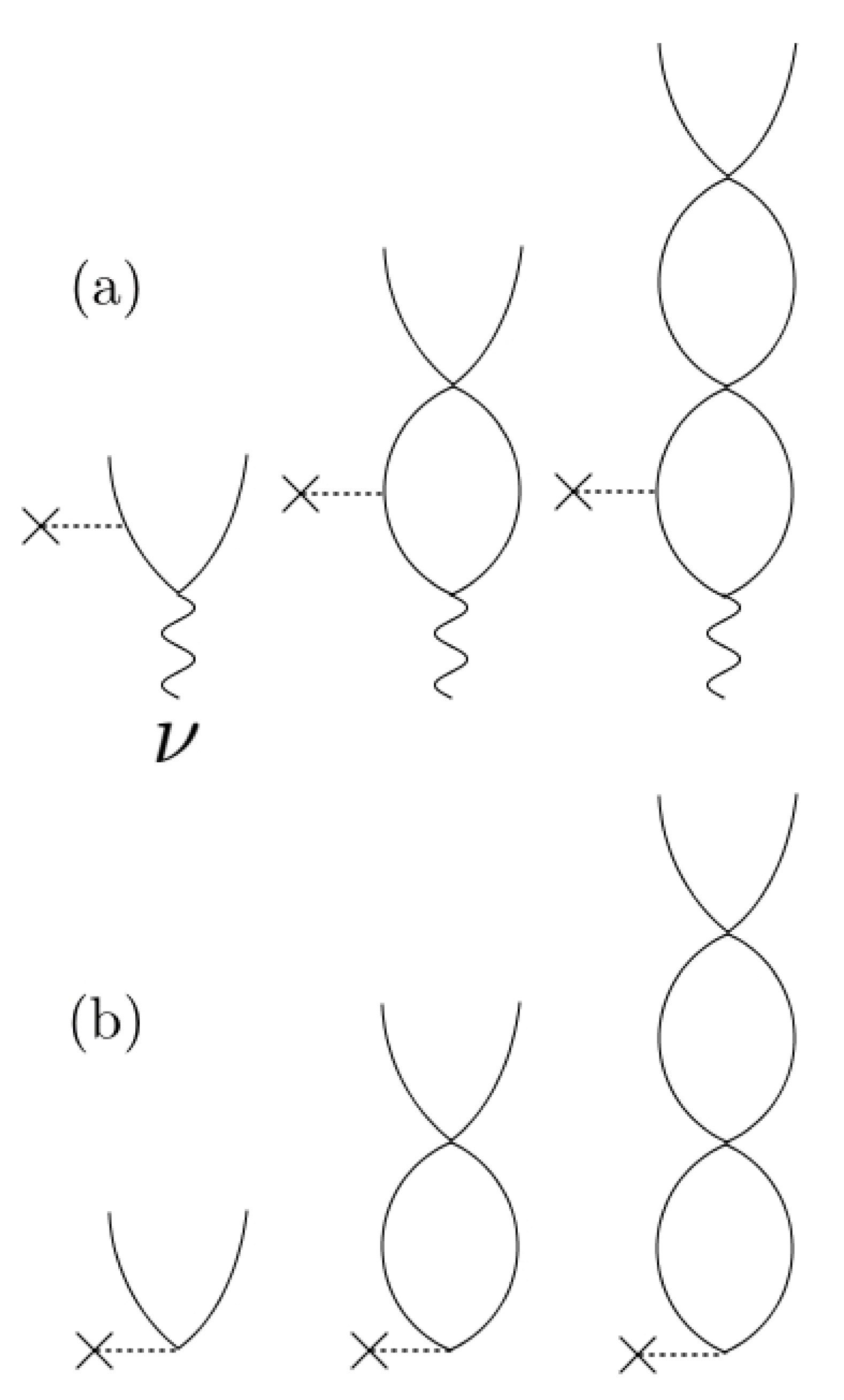
Figure 1: (a) The diagrams corresponding to $T$ matrix, Eq. (44), of the $(\gamma,n)$ reaction for the initial state $\ket{\nu}$ and the final state consisting one-quasiparticle configuration $n$ and the scattering neutron $p(E_{p})$. (b) Same as (a) but the case where the initial state is the ground state $\ket{0^{+}_{\rm gs}}$.

II.4 Concrete expressions for $(\gamma,n)$ and $(n,\gamma)$ cross sections

We perform numerical calculations under the assumption of spherical symmetry of the system, and describe the response with partial waves of the single-particle (quasiparticle) states and the multipolarity $LM$ of the total system. We specify the quasiparticle configuration of the odd-$N$ nucleus with $nlj$, and the escaping neutron with kinetic energy $\epsilon_{\rm kin}$ (or quasiparticle energy $E_{p}=|\lambda|+\epsilon_{\rm kin}$) and the partial wave quantum number $l^{{}^{\prime}}j^{{}^{\prime}}$. The final state $\ket{np(E_{p})}$ is $\ket{[nlj,\epsilon_{\rm kin}l^{{}^{\prime}}j^{{}^{\prime}}]_{LM}}=\sum_{mm^{{}^{\prime}}}\braket{jmj^{{}^{\prime}}m^{{}^{\prime}}|LM}\beta^{{\dagger}}_{nljm}\beta^{{\dagger}}_{E_{p}l^{{}^{\prime}}j^{{}^{\prime}}m^{{}^{\prime}}}\ket{0}$ with $L$ being the total angular momentum. Consequently we obtain the expression for the partial photoabsorption cross section for the specific channel of neutron decay as

$$\sigma^{\lambda}_{\nu L_{\nu}+\gamma\to[nlj,\epsilon_{\rm kin}l^{{}^{\prime}}j^{{}^{\prime}}]_{L}}(E_{\gamma}) =-\frac{f_{\lambda}(E_{\gamma})}{\pi(2L_{\nu}+1)}{\rm Im}\iiiint dr_{x}dr_{y}dr_{x^{{}^{\prime}}}dr_{y^{{}^{\prime}}}$$

$$\times\bar{\phi}^{T}_{nlj}(r_{y}){\cal V}^{\rm scf{\dagger}}_{L,l^{{}^{\prime}}j^{{}^{\prime}},lj}(r_{y},r_{x},\omega){\cal G}_{0c,l^{{}^{\prime}}j^{{}^{\prime}}}(r_{x},r_{x^{{}^{\prime}}},-E_{nlj}+\hbar\omega+i\epsilon){\cal V}^{\rm scf}_{L,l^{{}^{\prime}}j^{{}^{\prime}},lj}(r_{x^{{}^{\prime}}},r_{y^{{}^{\prime}}},\omega)\bar{\phi}_{nlj}(r_{y^{{}^{\prime}}}),$$ (45)

with

$${\cal V}^{\rm scf}_{L,l^{{}^{\prime}}j^{{}^{\prime}},lj}(r_{x},r_{y},\omega)={\cal F}_{L,l^{{}^{\prime}}j^{{}^{\prime}},lj}(r_{x},r_{y})+\langle l^{{}^{\prime}}j^{{}^{\prime}}||Y_{L}||lj\rangle\sum_{\beta}\frac{\delta{\cal U}}{\delta\rho_{\beta}}(r_{x})\frac{1}{r^{2}_{x}}\delta\rho_{\beta L}(r_{x},\omega)\delta(r_{x}-r_{y}).$$ (46)

Here ${\cal V}^{\rm scf}_{L,l^{{}^{\prime}}j^{{}^{\prime}},lj}(r_{x},r_{y},\omega)$ and ${\cal F}_{L,l^{{}^{\prime}}j^{{}^{\prime}},lj}(r_{x},r_{y})$ are matrix elements of $\hat{V}_{\rm scf}$ and $\hat{F}_{L}$ respectively (cf. Appendix B). $\hbar\omega=E_{\gamma}+E_{\nu}$ is the excitation energy of the states populated by the photoabsorption. The energy of emitted neutron is $\epsilon_{\rm kin}=-E_{nlj}+\hbar\omega-|\lambda|$.

Finally, using detailed balance we obtain the radiative neutron capture cross section for the reaction $\ket{[\Psi^{N_{odd}}_{nlj}\otimes\phi_{\epsilon_{\rm kin}l^{{}^{\prime}}j^{{}^{\prime}}}]_{L}}\to\ket{\nu L_{\nu}}+\gamma$:

$$\sigma^{\lambda}_{[nlj,\epsilon_{\rm kin}l^{{}^{\prime}}j^{{}^{\prime}}]_{L}\to\nu L_{\nu}+\gamma}(\epsilon_{\rm kin})=\frac{2L_{\nu}+1}{2j+1}\frac{E_{\gamma}}{2mc^{2}\epsilon_{\rm kin}}\sigma^{\lambda}_{\nu L_{\nu}+\gamma\to[nlj,\epsilon_{\rm kin}l^{{}^{\prime}}j^{{}^{\prime}}]_{L}}(E_{\gamma})$$ (47)

for an incident neutron with partial wave $l^{{}^{\prime}}j^{{}^{\prime}}$ and energy $\epsilon_{\rm kin}$ colliding on odd-$N$ nucleus with one-quasiparticle configuration $\beta^{{\dagger}}_{nlj}\ket{0}$, decaying to the excited state $\ket{\nu L_{\nu}M_{\nu}}$. The total cross section is obtained by summing all contributions of the partial waves $l^{{}^{\prime}}j^{{}^{\prime}}$ and the total angular momentum $L$ of the system.

III numerical examples

We shall demonstrate new features of the present theory with numerical calculations with a focus on roles of low-lying quadrupole and octupole collectivities as well as the pairing correlation. We shall discuss two examples, ${}^{91}{\rm Zn}(n,\gamma)^{92}{\rm Zn}$ and ${}^{89}{\rm Ge}(n,\gamma){}^{90}{\rm Ge}$. We have chosen these examples for the following reasons. First, these nuclei have small neutron separation energy of the order of $S_{1n}\sim 2-3$ MeV, and are near the $N=50$ waiting point on the $r$-process path and this area is of interest in terms of the weak $r$ process Surman et al. (2014). Second, the target odd-$N$ nuclei ${}^{91}{\rm Zn}$ and ${}^{89}{\rm Ge}$ are expected to have the valence neutron in the $2d_{3/2}$ orbit, and this situation is favorable for our discussion. As we show below, the QRPA calculation shows presence of many resonances with $L^{\pi}=2^{+}$ around the threshold energy, and a captured neutron in the $s$-wave combined with the valence neutron in the $d$-orbit will produce these resonances. Third, the QRPA calculation predicts low-lying collective $3_{1}^{-}$ state in ${}^{92}{\rm Zn}$ and ${}^{90}{\rm Ge}$. One may expect impact of the collectivity for the $E1$ transitions from the $2^{+}$ resonances to the $3^{-}_{1}$ state. Note also that these nuclei are expected to be spherical or only weakly deformed ($\beta_{2}<0.2$) in the ground state as many mean-field calculations predict Mas . We have performed calculations also for other isotopes in this mass region, and we focus below the cases with clear characteristic features.

III.1 setting

We use the Skyrme energy density functional model and the effective pairing interaction of the contact type to construct the self-consistent mean field, the HFB ground state, the residual interaction, and the excited states. The adopted Skyrme parameter sets are SkM^∗ Bartel and Quentin (1982) for ${}^{92}{\rm Zn}$ and SLy4 Chabanat et al. (1998) for ${}^{90}{\rm Ge}$, and the density-dependent delta interaction (DDDI),

$$v_{\rm pair,\tau}(\mathbf{r},\mathbf{r}^{{}^{\prime}})=v_{0}\frac{1-P_{\sigma}}{2}\left[1-\eta\left(\frac{\rho_{\tau}(\mathbf{r})}{\rho_{c}}\right)^{\alpha}\right]\delta(\mathbf{r}-\mathbf{r}^{{}^{\prime}}),$$ (48)

with $v_{0}=-458.4$ MeV, $\rho_{c}=0.08$ fm^-3 are used Matsuo and Serizawa (2010). The subscript $\tau$ indicates neutron or proton component. The cutoff energy of quasiparticle is $E_{\rm cut}=60$ MeV and the cutoff orbital angular momentum is $l_{\rm cut}=8$. The radial HFB equation is solved in a spherical box $r<R_{\rm max}$ with mesh $\Delta r=0.2$ fm in the box boundary condition $\phi(r=R_{\rm max})=0$ with $R_{\rm max}=20$ fm. The DDDI dimensionless parameter sets are fitted to the experimental pairing gaps of stable Zn and Ge isotopes; $\alpha=0.59,\eta=0.76$ for ${}^{92}{\rm Zn}$ and $\alpha=0.59,\eta=0.69$ for ${}^{90}{\rm Ge}$ with $\alpha$ given in Ref. Matsuo and Serizawa (2010).

The setting for the QRPA calculation is as follows. We adopt the Landau-Migdal approximation for the residual interaction in the linear response equation. Namely the residual particle-hole interaction is given by a contact force with the Landau-Migdal parameters $F_{0}(\mathbf{r}),F_{0}^{{}^{\prime}}(\mathbf{r})$, for which we use local density approximation. Under this approximation, we solve the linear response equation to obtain the fluctuations in the local density and the local pair density, and the corresponding local particle-hole and local pair fields for the induced field. As is often done in many works adopting the Landau-Migdal approximation, the residual interaction is multiplied by a renormalization factor $f$ so that the spurious dipole mode associated with the displacement motion appears at zero excitation energy. There is no experimental information on excited states of ${}^{92}{\rm Zn}$ and ${}^{90}{\rm Ge}$, which are the final states of the $\gamma$ transition. The lowest-lying $2^{+}$ state is observed at excitation energy 0.599 MeV in a neighbor nucleus ${}^{84}{\rm Zn}$ Shand et al. (2017), and at 0.527 MeV in ${}^{86}{\rm Ge}$ Miernik et al. (2013). In calculating the quadruple mode, we use a renormalization factor which reproduces these excitation energies. For other multipoles, we use the same value of $f$ as that of the dipole mode.

In order to obtain the density fluctuations and the induced field in the continuum spectrum above the neutron separation energy, we use the response function Eq. (A) in the Green’s function representation. Here the quasiparticle wave functions constructing Green’s function are connected to the Hankel functions at $R_{\rm max}$ in order to treat the unbound quasiparticle states with proper boundary conditions. The small imaginary constant $i\epsilon$ in the response and Green’s functions is set as $\epsilon=0.1$ MeV otherwise stated. The constant $\epsilon$ in the Green’s function in Eq. (II.4) for the $(\gamma,n)$ cross section is taken a very small value $\epsilon=10^{-8}$ MeV in order to calculate the scattering quasiparticle states with precise energy. The $\gamma$ transition is assumed to be $E1$ type.

III.2 ${}^{89}{\rm Ge}(n,\gamma)^{90}{\rm Ge}$

Quasiparticle states for ${}^{90}{\rm Ge}$ around the Fermi energy, obtained by the HFB calculation using the Skyrme SLy4 functional, are listed in Table 1. The neutron Fermi energy is $\lambda_{n}=-2.14$ MeV, and the bound quasineutron states are those associated with the orbits $3s_{1/2}$, $2d_{3/2}$, $2d_{5/2}$ and $1g_{7/2}$. The ground state of the neighbor odd-$N$ nucleus ${}^{89}{\rm Ge}$ is expected to have one-quasineutron configuration $3s_{1/2}$ or $2d_{3/2}$, which we denote ${}^{89}{\rm Ge}(1/2^{+})$ or ${}^{89}{\rm Ge}(3/2^{+})$ in the following. The neutron separation energy of ${}^{90}{\rm Ge}$ for channels decaying to ${}^{89}{\rm Ge}(1/2^{+})$ or ${}^{89}{\rm Ge}(3/2^{+})$ are then $S_{1n}(3s_{1/2})=E_{3s_{1/2}}+|\lambda_{n}|=2.84$ MeV, $S_{1n}(2d_{3/2})=E_{2d_{3/2}}+|\lambda_{n}|=3.31$ MeV, respectively. We calculate two cases of the $(n,\gamma)$ cross section, where the target state is ${}^{89}{\rm Ge}(1/2^{+})$ or ${}^{89}{\rm Ge}(3/2^{+})$.

Figure 2 shows the QRPA strength functions for the dipole, quadrupole and octupole excitations ($L^{\pi}=1^{-},2^{+},3^{-}$) of ${}^{90}{\rm Ge}$ for isoscalar, isovector, neutron and proton multipole operators. For the dipole ($L^{\pi}=1^{-}$), the isovector strength forms a broad continuous bump above the neutron separation energy, which may be regarded as soft dipole excitation. The peak at zero energy is the spurious displacement mode. For the quadrupole excitation ($L^{\pi}=2^{+}$), there exist many peaks in the energy region shown here. The lowest peak, corresponding to the $2^{+}_{1}$ state of ${}^{90}{\rm Ge}$ has excitation energy $E_{2^{+}_{1}}=0.880$ MeV and large isoscalar quadrupole strength, indicating a clear collective character of surface vibration. The collective nature is seen also in the forward and backward amplitudes ${X_{ij},Y_{ij}}$, listed in Table 2. We also note that that there exist peaks above the neutron separation energy, indicating presence of resonance states with $L^{\pi}=2^{+}$. We shall discuss the role of the resonances in the $(n,\gamma)$ reaction in the following. The octupole strength function shows a distinct low-lying peak with peak energy $E=0.881$ MeV. It has dominant isoscalar character indicating surface octupole vibration. The forward and backward amplitudes ${X_{ij},Y_{ij}}$ of this $3^{-}_{1}$ state is listed in Table 3. In the following we evaluate the cross sections for ${}^{89}{\rm Ge}(n,\gamma)^{90}{\rm Ge}$, where the final states of the $\gamma$ transition are the ground state, the $2^{+}_{1}$ state and the $3^{-}_{1}$ state of ${}^{90}{\rm Ge}$.

Table 1: Single-quasiparticle energies of the adopted Skyrme energy density functional SLy4 for ${}^{90}{\rm Ge}$. Quasiparticle states corresponding to bound Hartree-Fock orbits around the Fermi energy ($\lambda_{n}=-2.14,\lambda_{p}=-16.96$ MeV) are listed. Here the quasiparticle state $1g_{7/2}$, for instance, is the one which corresponds to the bound Hartree-Fock orbit $1g_{7/2}$.

neutrons	$E_{i}$ (MeV)		protons	$E_{i}$ (MeV)
$1g_{7/2}$	2.02		$1f_{7/2}$	5.40
$2d_{5/2}$	1.96		$2p_{1/2}$	2.69
$2d_{3/2}$	1.17		$1f_{5/2}$	2.11
$3s_{1/2}$	0.70		$2p_{3/2}$	1.80

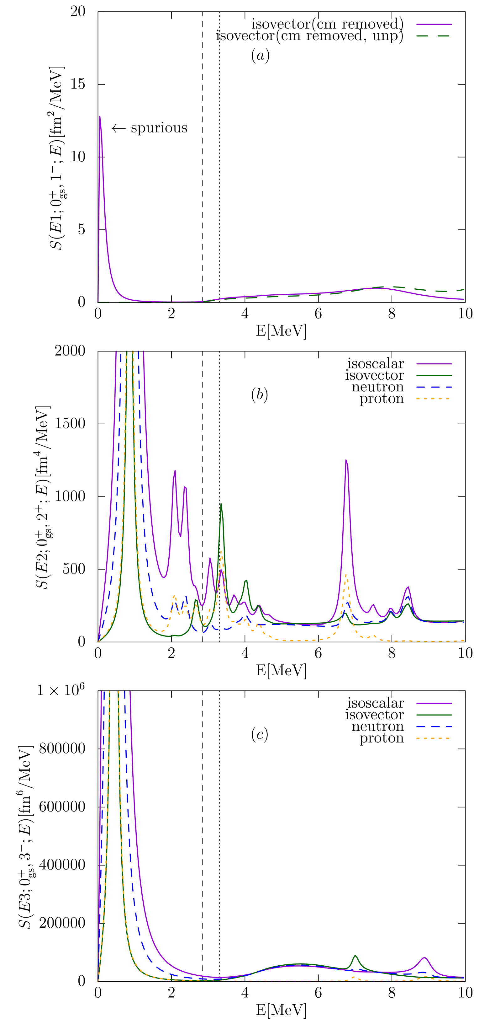
Figure 2: (a) The strength function for $L^{\pi}=1^{-}$ excited states in ${}^{90}{\rm Ge}$, calculated with $\epsilon=0.1$ MeV. The horizontal axis is the excitation energy of the $1^{-}$ states. The vertical dashed and dotted lines indicate one-neutron separation energies $S_{1n}(3s_{1/2})=2.84$ MeV and $S_{1n}(2d_{3/2})=3.31$ MeV, respectively. (b) and (c) Same as (a) but for $L^{\pi}=2^{+}$ and $3^{-}$ states, respectively.

Table 2: The QRPA forward and backward amplitudes $X_{ij},Y_{ij}$ of the $2^{+}_{1}$ state of ${}^{90}{\rm Ge}$. Two-quasiparticle configurations with large amplitude $|X_{ij}|>0.1$ are listed. The QRPA backward and forward amplitudes $X_{ij},Y_{ij}$ are calculated with use of the method of Ref. Shimoyama and Matsuo (2013) and discretized quasiparticle states obtained in the box boundary condition.

neutron config.	$X_{ij}$	$Y_{ij}$		proton config.	$X_{ij}$	$Y_{ij}$
$[2d_{3/2}][3s_{1/2}]$	-0.63	-0.17		$[2p_{3/2}][2p_{1/2}]$	-0.21	-0.12
$[1g_{7/2}][2d_{3/2}]$	-0.38	0.15		$[2p_{3/2}]^{2}$	-0.21	0.11
$[2d_{5/2}][3s_{1/2}]$	-0.31	0.099		$[1f_{5/2}]^{2}$	-0.20	0.11
$[2d_{3/2}]^{2}$	0.29	-0.087		$[1f_{5/2}][2p_{1/2}]$	0.20	-0.12
$[1g_{7/2}]^{2}$	0.22	-0.091		$[1f_{5/2}][2p_{3/2}]$	-0.16	-0.087
$[2d_{5/2}][2d_{3/2}]$	-0.21	-0.10		$[1f_{7/2}][2p_{3/2}]$	-0.14	0.096
$[1g_{7/2}][2d_{5/2}]$	-0.13	-0.077

Table 3: Same as Table 2 but for the $3^{-}_{1}$ state of ${}^{90}{\rm Ge}$. Two-quasiparticle configurations with the largest 10 amplitudes are listed. The label $c_{1}$ in $c_{1}h_{11/2}$ for example represents a continuum but discretized unbound quasiparticle state in the partial wave $h_{11/2}$. The numbering in $c_{i}$ is given according to the order of the quasiparticle energies for each partial wave.

neutron config.	$X_{ij}$	$Y_{ij}$		proton config.	$X_{ij}$	$Y_{ij}$
$[c_{1}h_{11/2}][2d_{5/2}]$	0.88	-0.66		$[1g_{9/2}][2p_{3/2}]$	0.64	-0.49
$[1g_{9/2}][c_{1}h_{11/2}]$	0.53	-0.45		$[1g_{9/2}][1f_{7/2}]$	0.42	-0.35
$[2p_{1/2}][1g_{7/2}]$	0.29	-0.25		$[1g_{9/2}][1f_{5/2}]$	-0.19	-0.15
$[1f_{5/2}][1g_{7/2}]$	-0.26	0.23		$[c_{2}i_{13/2}][1f_{7/2}]$	-0.19	0.17
$[c_{2}f_{7/2}][2d_{5/2}]$	-0.18	0.15		$[2d_{3/2}][2p_{3/2}]$	-0.18	-0.16
$[c_{2}f_{7/2}][3s_{1/2}]$	0.18	-0.14		$[1f_{7/2}][2d_{5/2}]$	-0.18	0.16
$[2p_{3/2}][2d_{3/2}]$	-0.18	-0.15		$[2d_{5/2}][2p_{3/2}]$	-0.17	0.15
$[c_{4}j_{15/2}][1g_{9/2}]$	-0.16	0.15		$[1g_{7/2}][1f_{5/2}]$	-0.17	0.15
$[1f_{7/2}][c_{3}i_{13/2}]$	-0.15	0.14		$[1f_{5/2}][2s_{1/2}]$	-0.16	-0.14
$[1f_{5/2}][2d_{3/2}]$	0.15	-0.13		$[1d_{5/2}][1h_{11/2}]$	-0.15	0.14

First we discuss the calculated $(n,\gamma)$ cross section for the $J^{\pi}=3/2^{+}$ configuration of ${}^{89}{\rm Ge}$ in the initial channel. Solid curves in Fig. 3 represent the cross section for the $E1$ transition to the ground state, the $2^{+}_{1}$ and the $3^{-}_{1}$ states of ${}^{90}{\rm Ge}$, i.e., for the reaction ${}^{89}{\rm Ge}(3/2^{+})+n\to^{90}{\rm Ge}({\rm g.s.},2^{+}_{1},3^{-}_{1})+\gamma$.

The dotted curves show another calculation in which the QRPA correlation is neglected in the excited continuum states (scattering states) while the final states of the $\gamma$ transition, i.e., the low-lying $2^{+}_{1}$ and $3^{-}_{1}$ in the present case, are constructed with the QRPA. Practically we drop off the induced field ${\cal V}_{\rm ind}$ in Eq. (II.4) in the calculation. In this case, the initial state with scattering neutron is approximated as an independent unbound quasineutron state, from which the $\gamma$ transition occurs directly. Hereafter we call this approximated calculation a semi-QRPA calculation since the QRPA correlation is taken into account only in the low-lying final states.

It is seen that the cross section for the transition to the $2^{+}_{1}$ state is larger than that to the ground state. The cross section to the $3^{-}_{1}$ state is the largest at low energy $\epsilon_{\rm kin}\mathop{\vbox{ \offinterlineskip\hbox{$<$}\hbox to7.7778pt{\hss\hbox{$\sim$}\hss}}}0.1$ MeV. It is noted that there would be no $3^{-}$ states (no negative parity states) below the threshold energy if there is no QRPA correlation.

Distinctive features are seen in the cross section for the transition to the $3^{-}_{1}$ state. It shows a very clear resonant behavior around $\epsilon_{\rm kin}\sim 0.03-0.07$ MeV in addition to many other (less significant) resonant peaks at higher energy $\epsilon_{\rm kin}\mathop{\vbox{ \offinterlineskip\hbox{$>$}\hbox to7.7778pt{\hss\hbox{$\sim$}\hss}}}0.3$ MeV. The cross section at this resonance $\epsilon_{\rm kin}\sim 0.03-0.07$ MeV is much larger than the cross sections for the ground state and for the $2^{+}_{1}$ final states by more than factor of $10^{2}$ and $10^{1}$. As seen in the comparison with the semi-QRPA result (dashed line), the resonance structure originates from the QRPA correlation (Fig. 4(b)) in the continuum excited states in ${}^{90}{\rm Ge}$. In fact, the resonance at $\epsilon_{\rm kin}\sim 0.03-0.07$ MeV corresponds to the peak at $E=3.35$ MeV of the quadrupole strength function for the $L^{\pi}=2^{+}$ excited states in ${}^{90}{\rm Ge}$ (Fig. 2(b)). Many of the other resonance structures also correspond to the peaks in the quadrupole strength function, e.g., the small peak at $\epsilon_{\rm kin}\sim 3.4$ MeV corresponds to a peak at $E\sim 6.7$ MeV.

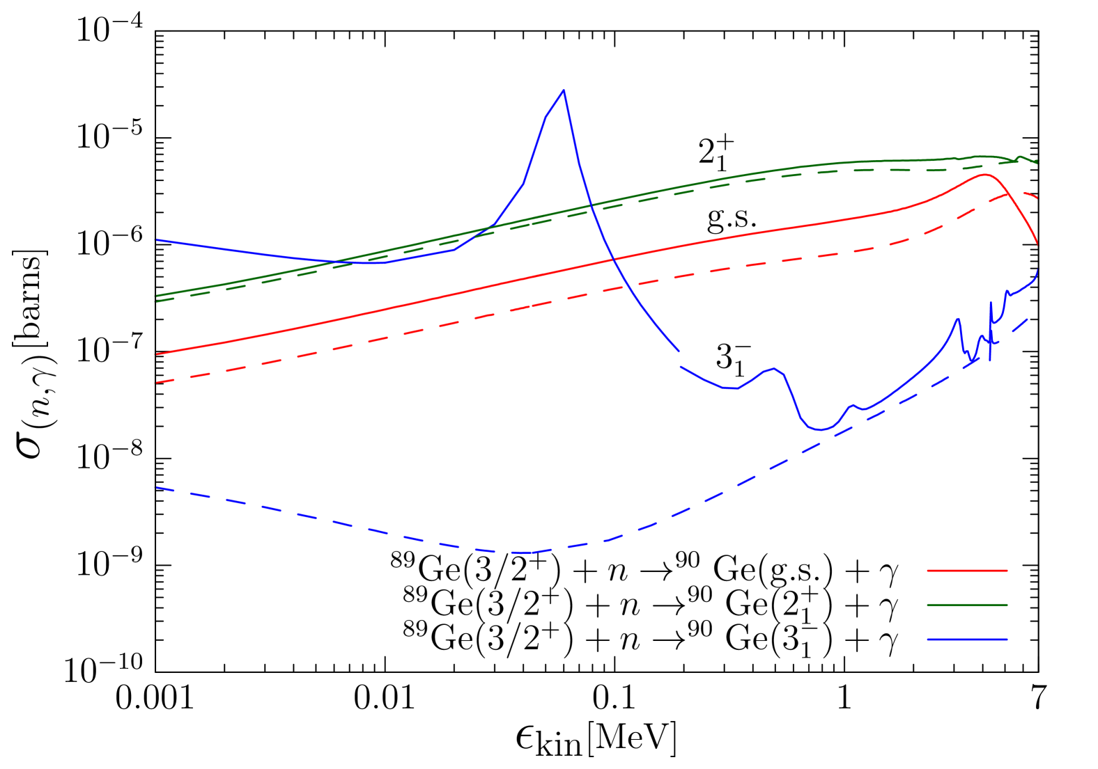
Figure 3: The calculated $(n,\gamma)$ cross sections for ${}^{89}{\rm Ge}(3/2^{+})+n\to^{90}{\rm Ge}+\gamma$ with $E1$ transitions populating different low-lying states in ${}^{90}{\rm Ge}$: the ground state, the quadrupole vibrational state $2^{+}_{1}$, and the octupole vibrational state $3^{-}_{1}$. The solid curves represent the results of the present theory while the dashed curves do the results of the semi-QRPA approximation, see text. The horizontal axis is kinetic energy $\epsilon_{\rm kin}$ of the incident neutron. The smoothing parameter $\epsilon$ is $0.1$ MeV, but smaller smoothing parameter $\epsilon=0.005$ MeV is used in low-energy region $\epsilon_{\rm kin}<0.2$ MeV for the transition to the $3^{-}_{1}$ state.

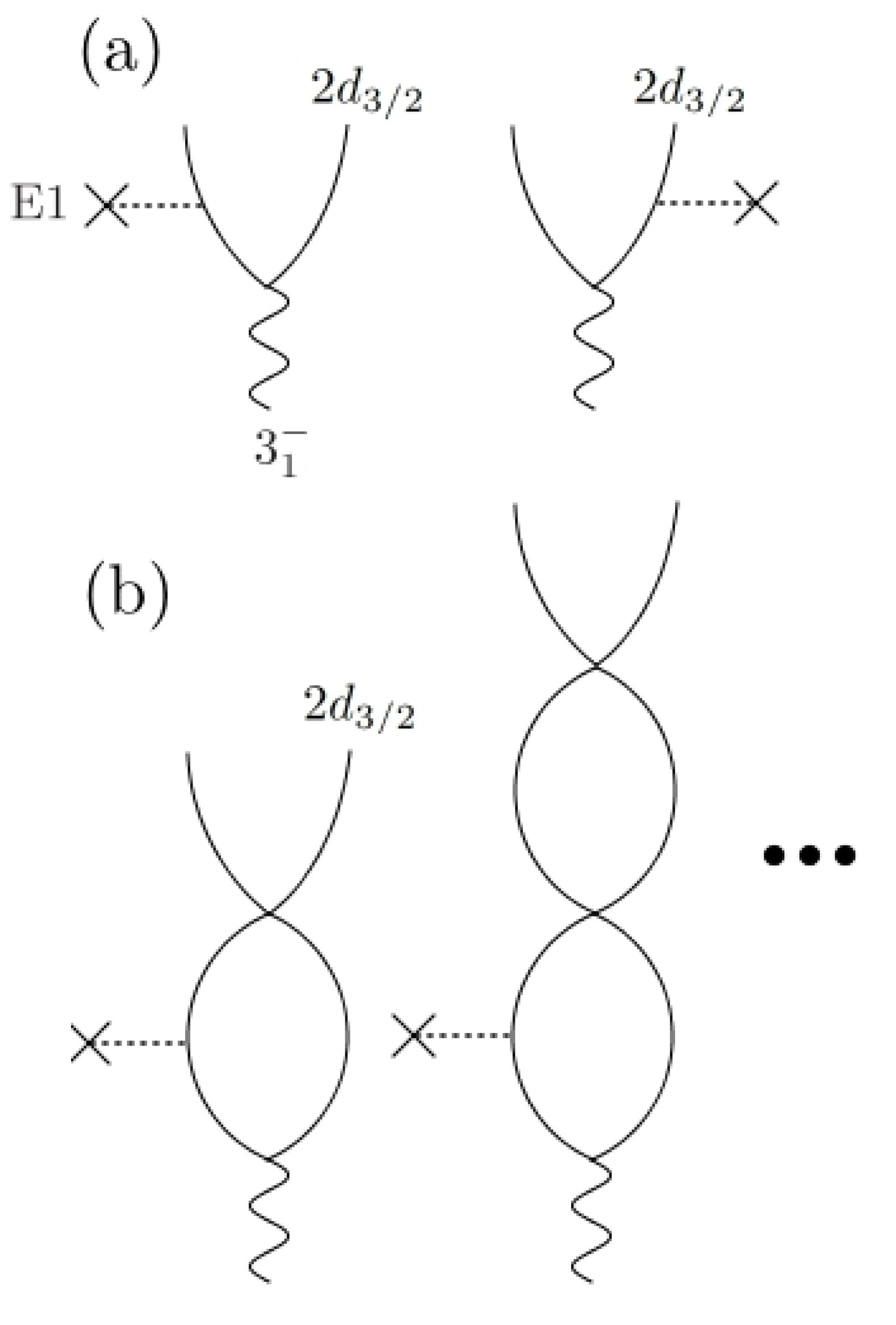
Figure 4: (a) Diagrams representing the $T$ matrix in the semi-QRPA approximation, where ${}^{89}{\rm Ge}$ has a one-quasineutron $2d_{3/2}$ configuration and the final state of the $\gamma$ transition is the $3^{-}_{1}$ state of ${}^{90}{\rm Ge}$ (b) Diagrams representing the QRPA correlation in the $T$ matrix.

The resonance $\epsilon_{\rm kin}\sim 0.03-0.07$ MeV is a collective state as seen in distribution of the forward amplitudes shown in Table 4. But it has a characteristic feature, different from the $2_{1}^{+}$ state of isoscalar surface vibration. A peak $E\approx 3.4$ MeV in the quadrupole strength function (Fig. 2(b)), which corresponds to the resonance at $\epsilon_{\rm kin}\sim 0.03-0.07$ MeV, exhibits isovector strength larger than isoscalar strength in contrast to other peaks. Figure 5(b) shows the transition density of this state. It is seen that neutrons oscillate with opposite phases in the inner and outer regions of the surface $r\sim 1.2\times 90^{1/3}=5.4$ fm, and that neutrons and protons oscillate with opposite phase in the outer region while they move coherently inside the surface. This behavior is the same as pygmy quadrupole resonance (PQR) predicted in Ref. Tsoneva and Lenske (2011), considered as an analogy of the pygmy dipole resonance. It is contrasting to the isoscalar surface vibration, i.e., the $2_{1}^{+}$ state whose transition density is shown in Fig. 5(a). In the following we refer the resonance at $E\approx 3.4$ MeV ($\epsilon_{\rm kin}\sim 0.03-0.07$ MeV) as a PQR.

The large impact of the PQR on the cross section has two origins. Because of the collectivity the PQR state couples to (consists of) a large number of two-quasiparticle configurations, including those in which one of the quasineutron is $2d_{3/2}$ (the configuration of ${}^{89}{\rm Ge}(3/2^{+})$) and the other is scattering quasineutron in $s,d_{3/2},d_{5/2}$ and $g_{7/2}$-waves. A consequence is seen in Fig. 6(c) showing the cross sections decomposed with respect to the partial waves of incoming neutrons for ${}^{89}{\rm Ge}(3/2^{+})+n\to^{90}{\rm Ge}(2^{+})\to^{90}{\rm Ge}(3^{-}_{1})+\gamma$, where the spin-parity $L^{\pi}=2^{+}$ of the excited states of ${}^{90}{\rm Ge}$ is specified. The enhanced cross section at the resonance around $\epsilon_{\rm kin}\sim 0.03-0.07$ MeV are seen in multiple partial waves $s_{1/2},d_{3/2}$ and $d_{5/2}$, rather than in single partial wave. In particular, the configuration including $s$-wave has a significant impact on the cross section since the $s$-wave becomes dominant at low energy.

Another important aspect of PQR is that the PQR includes proton two-quasiparticle configurations as well as neutron configurations as shown in Table 4. Therefore, the $E1$ operator acting on the proton component contribute to the transition between the PQR and the $3^{-}_{1}$ state: two-quasiproton configurations participate to rings in the middle part of the diagram Fig. 4(b). In addition, the isovector character of the PQR is preferable for enhancing the $E1$ transition as the $E1$ operator $\propto(N/A)\sum_{proton}(rY_{1m})-(Z/A)\sum_{neutron}(rY_{1m})$ is of isovector type.

Table 4: Same as Table 2 but for the PQR of ${}^{90}{\rm Ge}$. Two-quasiparticle configurations with large amplitude $|X_{ij}|>0.1$ are listed.

neutron config.	$X_{ij}$	$Y_{ij}$		proton config.	$X_{ij}$	$Y_{ij}$
$[2d_{5/2}][2d_{3/2}]$	0.49	-0.025		$[2p_{3/2}]^{2}$	-0.54	-0.020
$[1g_{7/2}][2d_{3/2}]$	0.38	0.038		$[1f_{5/2}]^{2}$	-0.27	-0.011
$[1g_{7/2}][2d_{5/2}]$	-0.18	-0.018		$[1f_{5/2}][2p_{3/2}]$	-0.24	0.002
$[1g_{7/2}]^{2}$	0.15	-0.028		$[1f_{5/2}][2p_{1/2}]$	0.17	0.004
$[2d_{5/2}][3s_{1/2}]$	0.13	0.034		$[2p_{3/2}][2p_{1/2}]$	-0.15	0.020

Figure 6(a) shows the cross section for ${}^{89}{\rm Ge}(3/2^{+})+n\to^{90}{\rm Ge}(1^{-})\to^{90}{\rm Ge}({\rm g.s.})+\gamma$ decaying to the ground state of ${}^{90}{\rm Ge}$ via $1^{-}$ excited states of the same nucleus. There is no sharp resonances in this reaction channel, reflecting the dipole strength function (Fig. 2) which shows only a broad continuum bump (the soft dipole excitation) at low excitation energy. Main components of the soft dipole excitation in the present example are two-quasineutron excitations consisting of bound $2d_{3/2}$ and $3s_{1/2}$ quasiparticles and unbound (scattering) $p$- and $f_{5/2}$-waves. The $p$-waves dominate the capture cross section at low kinetic energy due to the centrifugal barrier. Note that the QRPA correlation enhances the cross section by a factor of about two, indicating that the soft dipole excitation is not a pure single-particle transition Matsuo et al. (2005).

For the capture reaction with $E1$ transition to the $2_{1}^{+}$ state, the states with total angular momentum $L^{\pi}=1^{-},2^{-},3^{-}$ are relevant. Similarly to the transition to the ground state, there is no sharp resonances. An example is shown in Fig. 6(b) for the reaction channel ${}^{89}{\rm Ge}(3/2^{+})+n\to^{90}{\rm Ge}(3^{-})\to^{90}{\rm Ge}(2_{1}^{+})+\gamma$.

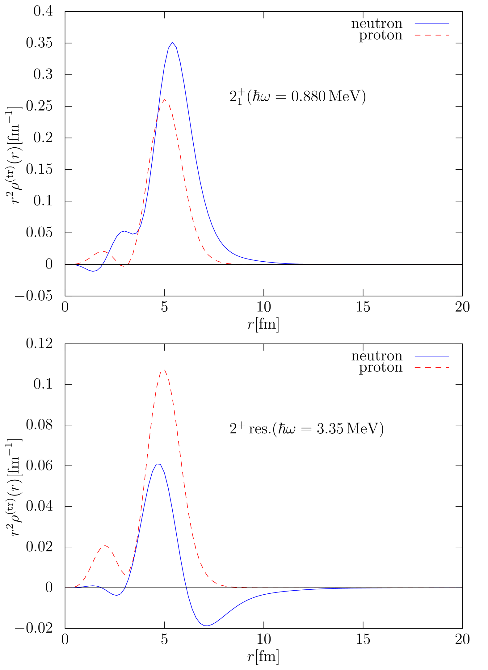
Figure 5: (a) The transition densities of neutrons and protons for the quadrupole vibrational state $2^{+}_{1}$ ($\hbar\omega=0.880$ MeV) of ${}^{90}{\rm Ge}$. (b) Same as (a) but for the pygmy quadrupole resonance (PQR, $\hbar\omega=3.35$ MeV) located just above the one-neutron separation energy.

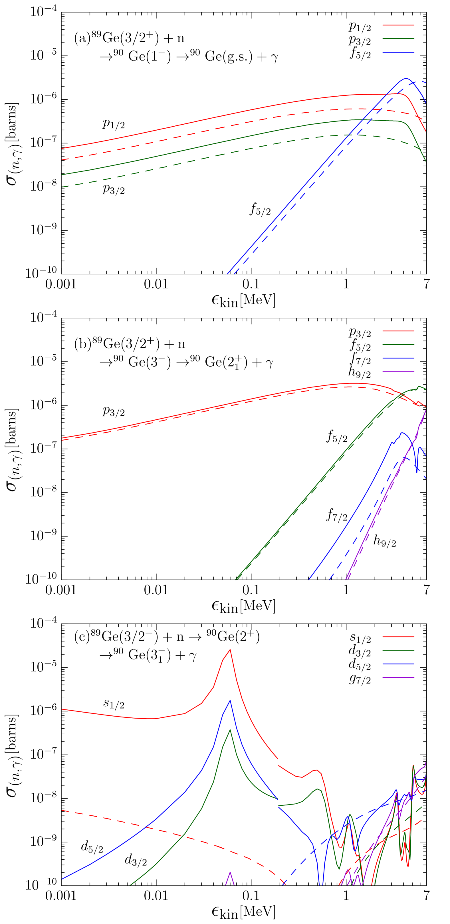
Figure 6: (a) The calculated partial $(n,\gamma)$ cross sections of the reaction ${}^{89}{\rm Ge}(3/2^{+})+n\to^{90}{\rm Ge}(1^{-})\to^{90}{\rm Ge}({\rm g.s.})+\gamma$ with $E1$ transition, plotted separately for different partial waves of the incident neutron. The solid curves represent the results of the present theory while the dashed curves do the results of the semi-QRPA approximation, see text. The horizontal axis is kinetic energy $\epsilon_{\rm kin}$ of the incident neutron. The smoothing parameter $\epsilon$ is $0.1$ MeV. (b) Same as (a) but for ${}^{89}{\rm Ge}(3/2^{+})+n\to^{90}{\rm Ge}(3^{-})\to^{90}{\rm Ge}(2^{+}_{1})+\gamma$. (c) Same as (a) but for ${}^{89}{\rm Ge}(3/2^{+})+n\to^{90}{\rm Ge}(2^{+})\to^{90}{\rm Ge}(3^{-}_{1})+\gamma$. Small smoothing parameter $\epsilon=0.005$ MeV is used in low-energy region $\epsilon_{\rm kin}<0.2$ MeV.

We shortly discuss the case where the configuration of the target nucleus ${}^{89}{\rm Ge}$ is the one-quasineutron state $3s_{1/2}$ with spin-parity $1/2^{+}$. Figure 7 shows $E1$ $(n,\gamma)$ cross section ${}^{89}{\rm Ge}(1/2^{+})+n\to^{90}{\rm Ge}({\rm g.s.},2^{+}_{1},3^{-}_{1})+\gamma$. In this case, we only see a tiny resonance behavior: the small peak at $\epsilon_{\rm kin}=0.5$ MeV in the cross section for the transition to the $3^{-}_{1}$ state is caused by the PQR in the $2^{+}$ states. In this case, the $s$-wave capture for the path ${}^{89}{\rm Ge}(1/2^{+})+n\to^{90}{\rm Ge}(2^{+})\to^{90}{\rm Ge}(3^{-}_{1})+\gamma$ is prohibited due to the angular momentum conservation. Only the $d$-waves can form $2^{+}$ states, making the cross section very small.

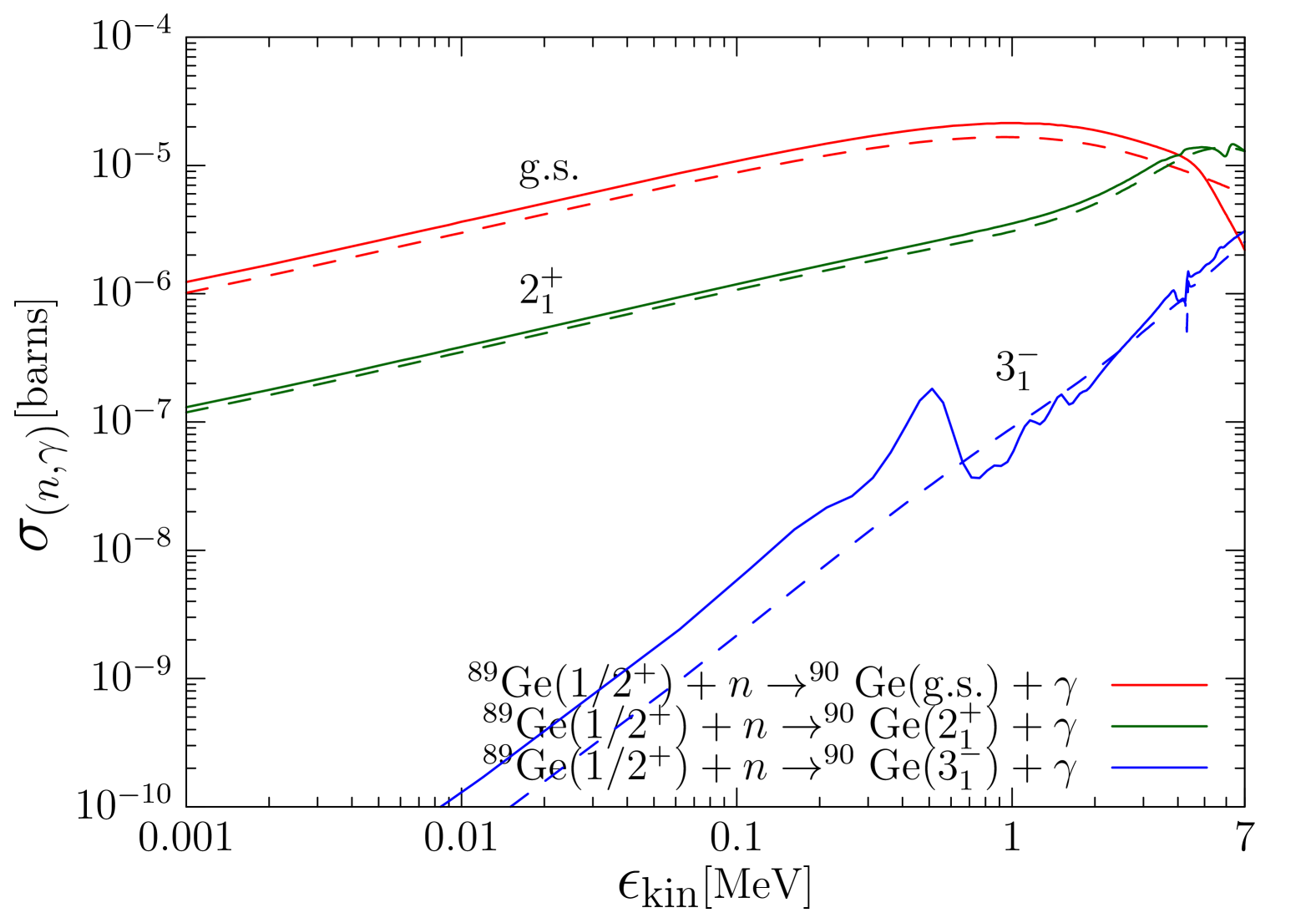
Figure 7: Same as Fig. 3 but for ${}^{89}{\rm Ge}(1/2^{+})+n\to^{90}{\rm Ge}+\gamma$. The smoothing parameter $\epsilon$ is $0.1$ MeV.

III.3 ${}^{91}{\rm Zn}(n,\gamma)^{92}{\rm Zn}$

The low-lying quasiparticle states in ${}^{92}{\rm Zn}$ obtained with SkM^∗ are listed in Table 5. Since only the state $2d_{3/2}$ is a bound quasineutron state, we assume that the ground state of ${}^{91}{\rm Zn}$ has the one-quasineutron configuration $2d_{3/2}$ with total spin-parity $3/2^{+}$. We then describe $(n,\gamma)$ reaction in which a neutron is impinging on the ground state ${}^{91}{\rm Zn}(3/2^{+})$. Note that a bound Hartree-Fock orbit $3s_{1/2}$ located just below the Fermi energy becomes a resonant quasiparticle state, called quasiparticle resonance Dobaczewski et al. (1996); Bennaceur et al. (1999); Balgac , which is embedded in continuum just above (by $\sim 0.2$ MeV) the threshold energy $E=|\lambda_{n}|=1.43$ MeV.

Figure 8 shows the dipole, quadrupole and octupole strength functions for multipole operators, calculated for $1^{-},2^{+},3^{-}$ excited sates in ${}^{92}{\rm Zn}$ in the excitation energy range $E=0-10$ MeV. Significant low-energy peaks are seen at $E_{2^{+}_{1}}=0.380$ and $E_{3^{-}_{1}}=0.950$ MeV in the quadrupole and octupole strength functions, respectively. These are collective states as evident from the forward and backward amplitudes $X_{ij},Y_{ij}$, listed in Tables 6 and 7.

Table 5: Single-quasiparticle energies of the adopted Skyrme energy density functional SkM^∗ for ${}^{92}{\rm Zn}$, obtained with the box boundary condition. Quasiparticle states corresponding to bound Hartree-Fock orbits around the Fermi energy ($\lambda_{n}=-1.43,\lambda_{p}=-18.40$ MeV) are listed. Quasineutron states $3s_{1/2},1g_{7/2}$ and $2d_{5/2}$, whose energies are larger than the threshold $|\lambda_{n}|=1.43$ MeV, are quasiparticle resonances.

neutrons	$E_{i}$ (MeV)		protons	$E_{i}$ (MeV)
$2d_{5/2}$	3.03		$1g_{9/2}$	5.79
$1g_{7/2}$	1.77		$1f_{7/2}$	4.53
$3s_{1/2}$	1.67		$2p_{1/2}$	2.65
$2d_{3/2}$	0.91		$1f_{5/2}$	2.35
			$2p_{3/2}$	1.34

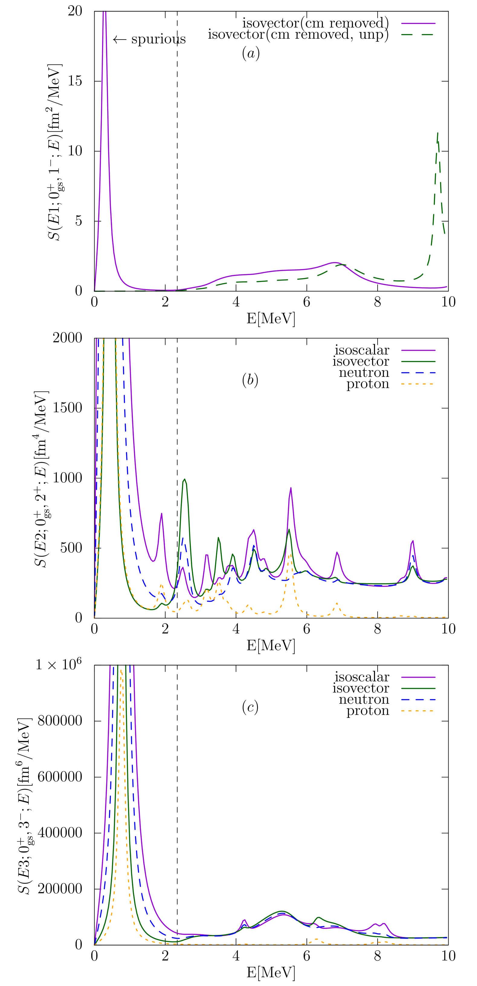
Figure 8: (a) The strength function for $L^{\pi}=1^{-}$ excited states in ${}^{92}{\rm Zn}$, calculated with $\epsilon=0.1$ MeV. The horizontal axis is the excitation energy of the $1^{-}$ states. The vertical dashed line is one neutron separation energy $S_{1n}(2d_{3/2})=2.34$ MeV. (b) and (c) Same as (a) but for $L^{\pi}=2^{+}$ and $3^{-}$ states.

Table 6: Same as Table 2 but for the $2^{+}_{1}$ of ${}^{92}{\rm Zn}$. Two-quasiparticle configurations with the largest 10 amplitudes are listed. See also the caption in Table 3.

neutron config.	$X_{ij}$	$Y_{ij}$		proton config.	$X_{ij}$	$Y_{ij}$
$[1g_{7/2}][2d_{3/2}]$	0.76	-0.53		$[2p_{3/2}]^{2}$	-0.44	0.31
$[2d_{3/2}]^{2}$	0.47	-0.27		$[2p_{3/2}][2p_{1/2}]$	-0.35	-0.27
$[1g_{7/2}]^{2}$	0.38	-0.27		$[1f_{7/2}][2p_{3/2}]$	-0.34	0.29
$[c_{1}h_{11/2}]^{2}$	-0.31	0.23		$[1f_{5/2}][2p_{3/2}]$	-0.24	-0.18
$[2d_{3/2}][3s_{1/2}]$	0.26	0.16		$[1f_{5/2}][2p_{1/2}]$	0.23	-0.18
$[c_{2}i_{13/2}][1g_{9/2}]$	-0.15	0.14		$[1f_{5/2}]^{2}$	-0.20	0.15
$[1f_{7/2}][c_{1}h_{11/2}]$	-0.15	0.14		$[1h_{11/2}][1f_{7/2}]$	-0.17	0.17
$[1g_{7/2}][2d_{5/2}]$	-0.12	-0.099		$[1d_{5/2}][1g_{9/2}]$	-0.12	0.11
$[2d_{5/2}][2d_{3/2}]$	0.11	0.078		$[1f_{7/2}][1f_{5/2}]$	0.11	0.095
$[c_{3}i_{13/2}][1g_{9/2}]$	-0.11	0.11

Table 7: Same as Table 2 but for the $3^{-}_{1}$ of ${}^{92}{\rm Zn}$. Two-quasiparticle configurations with the largest 10 amplitudes are listed. See also the caption in Table 3.

neutron config.	$X_{ij}$	$Y_{ij}$		proton config.	$X_{ij}$	$Y_{ij}$
$[c_{1}h_{11/2}][2d_{5/2}]$	0.73	-0.51		$[1g_{9/2}][2p_{3/2}]$	0.53	-0.39
$[1g_{9/2}][c_{1}h_{11/2}]$	0.45	-0.36		$[1g_{9/2}][1f_{7/2}]$	0.42	-0.35
$[c_{1}d_{5/2}][c_{1}h_{11/2}]$	-0.30	0.21		$[c_{1}i_{13/2}][1f_{7/2}]$	-0.19	0.18
$[c_{1}h_{11/2}][1g_{7/2}]$	0.24	0.14		$[1f_{5/2}][2s_{1/2}]$	-0.19	-0.16
$[2p_{1/2}][1g_{7/2}]$	0.23	-0.20		$[1f_{7/2}][2d_{5/2}]$	-0.17	0.15
$[c_{2}f_{7/2}][3s_{1/2}]$	0.19	-0.14		$[1d_{3/2}][2p_{3/2}]$	-0.16	-0.13
$[1f_{5/2}][1g_{7/2}]$	0.19	-0.15		$[1f_{5/2}][1d_{3/2}]$	-0.16	0.13
$[c_{1}f_{7/2}][3s_{1/2}]$	0.18	-0.12		$[1d_{5/2}][1h_{11/2}]$	-0.15	0.14
$[c_{3}h_{9/2}][2d_{3/2}]$	0.16	-0.14		$[2d_{3/2}][2p_{3/2}]$	-0.15	-0.13
$[c_{2}f_{7/2}][2d_{5/2}]$	-0.16	0.12		$[2d_{5/2}][2p_{3/2}]$	-0.14	0.12

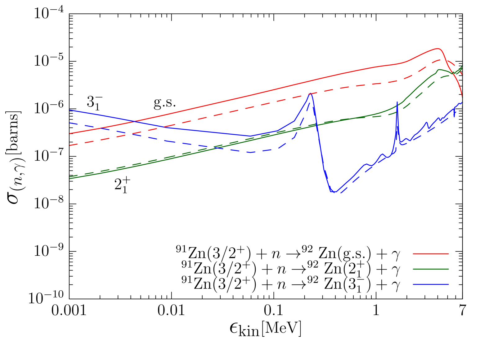
Figure 9: Same as Fig. 3 but for ${}^{91}{\rm Zn}(3/2^{+})+n\to^{92}{\rm Zn}+\gamma$. The smoothing parameter $\epsilon$ is $0.1$ MeV.

Figure 9 shows calculated capture cross section for the $(n,\gamma)$ reaction ${}^{91}{\rm Zn}(3/2^{+})+n\to^{92}{\rm Zn}({\rm g.s.},2^{+}_{1},3^{-}_{1})+\gamma$ in which the final states of the $E1$ transition are the low-lying $2^{+}_{1}$ and $3^{-}_{1}$ states as well as the ground state of ${}^{92}{\rm Zn}$. The cross section for the transition to the $3^{-}_{1}$ state is noticeable as it exhibits an apparent resonant behavior at $\epsilon_{\rm kin}\sim 0.2$ MeV. This resonance arises from the excited $2^{+}$ state of ${}^{92}{\rm Zn}$ in the continuum, corresponding to a peak at $E\sim 2.6$ MeV in the quadrupole strength function (Fig. 8(b)). We notice further that the cross section increases with decreasing the neutron energy below the resonance energy $\epsilon_{\rm kin}\mathop{\vbox{ \offinterlineskip\hbox{$<$}\hbox to7.7778pt{\hss\hbox{$\sim$}\hss}}}0.1$ MeV, and becomes larger than the cross section for the transition to the ground state. There exist also many other resonant behaviors at higher energy $\epsilon_{\rm kin}=1-7$ MeV. These resonances correspond to the peaks in the range of $2-9$ MeV in the quadrupole strength function and non-correlated $3^{+}$, correlated $4^{+}$ peaks.

We note that the resonance at $\epsilon_{\rm kin}\sim 0.2$ MeV has different structure from the one we have discussed for ${}^{90}{\rm Ge}$, in which case the QRPA correlation played the key role to produce the resonant state, i.e., the PQR. This is seen from a comparison with the semi-QRPA calculation (dotted curve). There exists essentially the same resonance behavior at $\epsilon_{\rm kin}\sim 0.2$ MeV in the semi-QRPA calculation although the QRPA correlation gives only a weak enhancement of the cross section around this resonance (and at lower energies) by a factor of about two. Figure 10(a) shows decomposition of the cross section with respect to the partial waves of the incident neutron. The resonance structure at $\epsilon_{\rm kin}\sim 0.2$ MeV appears only in the $s$-wave neutron while it is not seen for the $d$-waves, in which a peak structure would have appeared if the origin of the resonance is the QRPA correlation. The above observations suggest that the resonance at $\epsilon_{\rm kin}\sim 0.2$ MeV is the one with single-particle character associated with the scattering $s$-wave neutron state. Indeed the peak of the dotted line exactly corresponds to the quasineutron resonance with $E\approx 2.58$ MeV, originating from the $3s_{1/2}$ orbit.

Roles of the $3s_{1/2}$ quasineutron resonance may be explained in terms of the diagrams shown in Fig. 11. The initial state of the reaction corresponds to the top part of the diagram, and it consists of the scattering $s$-wave quasineutron and $2d_{3/2}$ quasineutron state. This configuration has $E1$ matrix elements to the the $3_{1}^{-}$ state (represented by the wavy line in the bottom part of the diagram). There are two contributions, in which the $E1$ operator acts on the $s$-wave neutron and the $2d_{3/2}$ quasineutron state, corresponding to the diagrams (a) and (b), respectively. The $E1$ matrix elements are expressed as

$$\sum_{c}\langle s_{1/2}|E1|cp_{3/2}\rangle X_{cp_{3/2},d_{3/2}}^{3_{1}^{-}} \quad{\rm for\ (a)},$$

$$\sum_{c}\langle 2d_{3/2}|E1|cf_{5/2}\rangle X_{s_{1/2},cf_{5/2}}^{3_{1}^{-}} \quad{\rm for\ (b)},$$ (49)

where $X_{ij}^{3_{1}^{-}}$ is the forward amplitude of two-quasiparticle configuration $ij$ in the $3_{1}^{-}$ state. Note that the two-quasineutron configurations $[cp_{3/2}\otimes 2d_{3/2}]_{3^{-}}$ contribute to the diagram (a) while $[s_{1/2}\otimes cf_{5/2}]_{3^{-}}$ for (b). Here $s_{1/2}$ is the scattering $s$-wave quasineutron, and $cp_{3/2}$ and $cf_{5/2}$ denote the unbound quasineutron states (labeled with ”$c$”) with quantum numbers $p_{3/2}$ and $f_{5/2}$. The above two-quasineutron components are present in the $3_{1}^{-}$ state due to a large collectivity of this state although the associated amplitudes $X_{ij}$ are small ($|X_{ij}|<0.1$).

Figure 10(b) shows cross sections in which the contributions from diagrams (a) and (b) are calculated separately. It is seen that both components contribute to the resonance structure, but in different ways. The diagram (b) forms a peak structure at the resonance energy while (a) contributes to the cross section with different signs depending on whether the energy of incident neutron is above or below the peak energy.

To understand this we note that $[s_{1/2}\otimes cf_{5/2}]_{3^{-}}$ components in the low-lying $3_{1}^{-}$ state contribute to (b) while $[cp_{3/2}\otimes 2d_{3/2}]_{3^{-}}$ components are relevant to (a). For (b), the forward amplitudes $X_{ij}$ of the $[s_{1/2}\otimes cf_{5/2}]_{3^{-}}$ components become large in Eq. (49) in the case when the scattering $s_{1/2}$ quasineutron is on the resonance. (In this case two-quasineutron configuration $[s_{1/2}\otimes cf_{5/2}]_{3^{-}}$ becomes that of a particle-hole character, a preferable feature for the vibrational $3^{-}_{1}$ state. The $3s_{1/2}$ quasineutron resonance has a hole character while unbound $cf_{5/2}$ has a particle character.) Hence the diagram (b) forms a peak at the resonance. For (a), relevant $E1$ matrix element is

$$\langle s_{1/2}|E1|cp_{3/2}\rangle =\frac{1}{2}\int dx\phi^{{\dagger}}_{s_{1/2}}(x){\cal M}_{E1}(x)\phi_{cp_{3/2}}(x)$$

$$=\frac{1}{2}\int dxf_{E1}(x)\left(\varphi^{*}_{s_{1/2},1}(x)\varphi_{cp_{3/2},1}(x)-\phi^{*}_{s_{1/2},2}(x)\phi_{cp_{3/2},2}(x)\right),$$ (50)

for which the the upper component $\varphi^{*}_{s_{1/2},1}(x)$ of the $s_{1/2}$ quasineutron (scattering neutron) gives dominant contribution as the unbound quasineutron state $cp_{3/2}$ has dominant upper component $|\varphi_{cp_{3/2},1}(x)|\gg|\varphi_{cp_{3/2},2}(x)|$. The upper component $\varphi_{s_{1/2},1}(x)$ of the $s_{1/2}$ quasiparticle is a scattering wave, and its amplitude changes sign depending on below or above the resonance energy, and hence contribution of the diagram (a) also changes sign accordingly.

The components of (a) and (b) contribute coherently (destructively) to the cross section below (above) the resonance peak, and this gives a large enhancement of the capture cross section at the lower tail of the resonance. We note that the diagram (b) is not usually considered in the single-particle neutron capture model because it only takes into account an incident neutron directly decaying to a bound single-particle orbit.

Summarizing, the resonant behavior at $\epsilon_{\rm kin}\sim 0.2$ MeV and the enhancement of the cross section at very low energy originate from a combined effect of the quasiparticle resonance in the $s$-wave scattering neutron and the collectivity of the low-lying $3_{1}^{-}$ state.

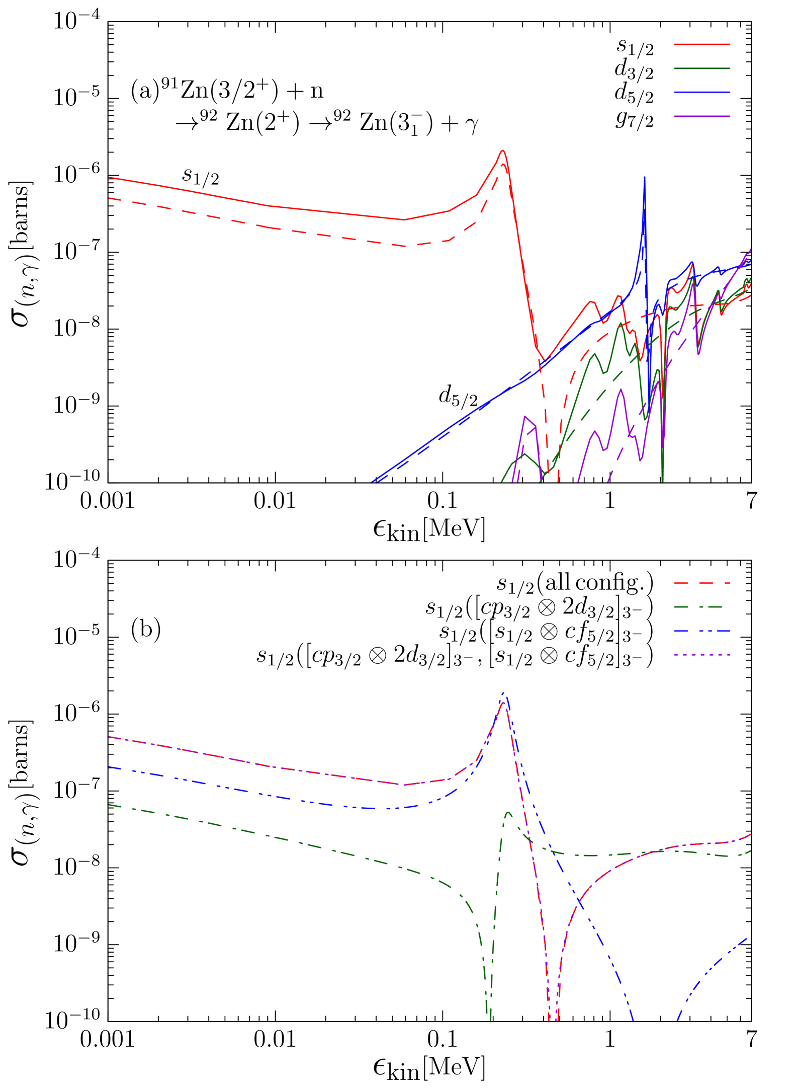
Figure 10: (a) The calculated partial $(n,\gamma)$ cross sections for the specific channel ${}^{91}{\rm Zn}(3/2^{+})+n\to^{92}{\rm Zn}(2^{+})\to^{92}{\rm Zn}(3^{-}_{1})+\gamma$ with $E1$ transition, plotted separately for different partial waves of the incident neutron. The solid curves represent the results of the present theory while the dashed curves do the results of the semi-QRPA approximation, see text. (b) The calculated semi-QRPA partial $(n,\gamma)$ cross sections where scattering neutron is limited to $s$-wave and two-quasineutron configurations are limited to $[cp_{3/2}\otimes 2d_{3/2}]_{3^{-}}$, $[s_{1/2}\otimes cf_{5/2}]_{3^{-}}$ or both. The horizontal axis is kinetic energy $\epsilon_{\rm kin}$ of the incident neutron. The smoothing parameter $\epsilon$ is $0.1$ MeV.

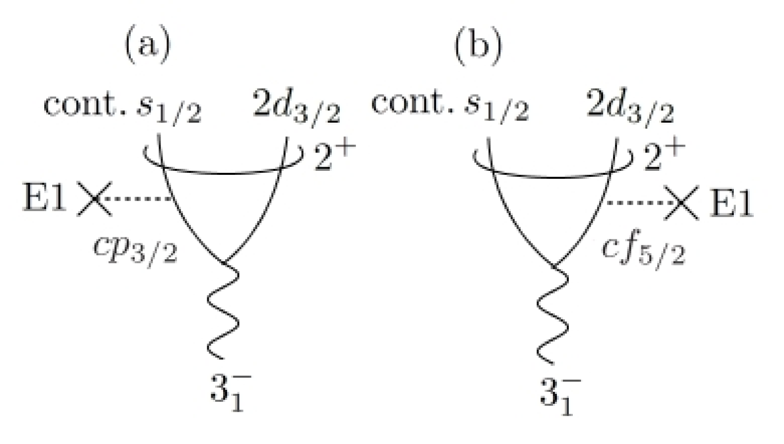
Figure 11: Diagrams in the semi-QRPA representing $s$-wave capture ${}^{91}{\rm Zn}(3/2^{+})+n_{s_{1/2}}\to^{92}{\rm Zn}(2^{+})\to^{92}{\rm Zn}(3^{-}_{1})+\gamma$ with $E1$ transition.

IV conclusions

The cQRPA enables one to describe collective excitations which decay through emission of a nucleon. Taking this advantage of the cQRPA, we have formulated a prototype theory previously Matsuo (2015) with which one can calculate the cross section of radiative neutron capture reaction on neutron-rich nuclei, relevant to $r$-process nucleosynthesis. In this prototype formulation, however, we have restricted ourselves to the case where the final state of $\gamma$ transition is the ground state of an even-even nucleus. In the present study, we have extended the formulation of Ref. Matsuo (2015) by incorporating the method of Ref. Saito and Matsuo (2023) that allows to describe the $\gamma$ transitions populating low-lying excited states such as surface vibrational $2_{1}^{+}$ and $3_{1}^{-}$ states. In the present framework, there appear resonances of collective and non-collective characters at low excitation energy near the threshold of neutron separation. Contributions of the resonances to the $(n,\gamma)$ cross section are taken into account in a consistent way together with direct transitions from scattering neutron state.

We have demonstrated the new features of the theory by presenting numerical calculations performed for reactions on neutron-rich open-shell nuclei in the region with $A\sim 90$ ( $N>50$, $Z>28$ ) with $S_{1n}\sim 2$ MeV: ${}^{89}{\rm Ge}(n,\gamma)^{90}{\rm Ge}$ and ${}^{91}{\rm Zn}(n,\gamma)^{92}{\rm Zn}$, in which $E1$ $\gamma$ transition to the ground state or low-lying excited states $2^{+}_{1},3^{-}_{1}$ are evaluated. The example of germanium is a case where a collective state having the character of the pygmy quadrupole resonance (PQR) appears in ${}^{90}{\rm Ge}$ just above the neutron separation energy. The resonance brings about a significant peak in the capture cross section as well as enhancement at very low energy. Here the enhanced cross section occurs for the transition to the low-lying $3^{-}_{1}$ state of the octupole vibration. Collectivities in the PQR and the octuple $3_{1}^{-}$ state play key roles.

The case of zirconium provides an example in which another type of resonance shows up. The neutron $3s_{1/2}$ orbit, which is an occupied bound orbit in the Hartree-Fock approximation, becomes with the neutron pairing a resonant quasiparticle state coupled to scattering neutron in the $s$-wave. This quasiparticle resonance contributes also to the cross section of ${}^{91}{\rm Zn}(n,\gamma)^{92}{\rm Zn}$, especially for the transition to the octupole $3^{-}_{1}$ state in ${}^{92}{\rm Zn}$. Note that the $E1$ transition from a $s$-wave is possible only to $p$-wave orbits, but there is no bound $p$-orbits around the $N\sim 60$ Fermi energy. Thanks to the collectivity, the octupole $3^{-}_{1}$ state contains a large number of two-quasineutron configurations, including those with unbound $p$-wave orbits, through which the $E1$ transition becomes possible.

The numerical examples point to new resonance mechanisms in the low-energy radiative neutron capture on neutron-rich nuclei. However, quantitative aspects should be taken with reservation as the results depend on the Skyrme and pairing parameters. Dependence on these parameters will be discussed in a forthcoming paper. In the present study, we have evaluated the $E1$ transitions. Inclusion of $M1$ component, another dominant transition, is straightforward. For systematic description of the $(n,\gamma)$ reaction, extension to other types of target nuclei, e.g., the proton-odd and even-even nuclei, is necessary, and it is also in progress.

V Acknowledgments

The numerical calculations were performed on the supercomputer HPE SGI8600 in the Japan Atomic Energy Agency. This work was supported by the JSPS KAKENHI (Grant No. 20K03945 and No. 24K07014).

Appendix A linear response equations

The generalized density matrix is defined and evaluated as

$${\cal R}(x,y)=\begin{pmatrix}\langle\psi^{{\dagger}}(y)\psi(x)\rangle&\langle\psi(\tilde{y})\psi(x)\rangle\\ \langle\psi^{{\dagger}}(y)\psi^{{\dagger}}(\tilde{x})\rangle&\langle\psi(\tilde{y})\psi^{\dagger}(\tilde{x})\rangle\\ \end{pmatrix}=\sum_{i}\bar{\phi}_{\tilde{i}}(x)\bar{\phi}^{\dagger}_{\tilde{i}}(y).$$ (51)

Its fluctuation under the perturbing field $\hat{V}_{\rm scf}$ is then given as

$$\delta{\cal R}(x,y,\omega) =\sum_{i}\delta\bar{\phi}_{\tilde{i}}(x,\omega)\bar{\phi}^{\dagger}_{\tilde{i}}(y)+\bar{\phi}_{\tilde{i}}(x)\delta\bar{\phi}^{\dagger}_{\tilde{i}}(y,-\omega)$$

$$=\iint dx^{{}^{\prime}}dy^{{}^{\prime}}\sum_{i}{\cal G}_{0}(x,x^{{}^{\prime}},-E_{i}+\hbar\omega+i\epsilon){\cal V}_{\rm scf}(x^{{}^{\prime}},y^{{}^{\prime}},\omega)\bar{\phi}_{\tilde{i}}(y^{{}^{\prime}})\bar{\phi}^{\dagger}_{\tilde{i}}(y)$$

$$+\iint dx^{{}^{\prime}}dy^{{}^{\prime}}\sum_{i}\bar{\phi}_{\tilde{i}}(x)\bar{\phi}^{\dagger}_{\tilde{i}}(x^{{}^{\prime}}){\cal V}_{\rm scf}(x^{{}^{\prime}},y^{{}^{\prime}},\omega){\cal G}_{0}(y^{{}^{\prime}},y,-E_{i}-\hbar\omega-i\epsilon),$$ (52)

where ${\cal G}_{0}(E)=(E-{\cal H}_{0})^{-1}$ is the quasiparticle Green’s function defined with the $2\times 2$ Hamiltonian ${\cal H}_{0}$ for the HFB equation, Eq. (12). Each component of the generalized density matrix fluctuation is accordingly given by

$$\delta\rho_{\alpha}(x,y,\omega)={\rm Tr}{\cal A}_{\alpha}\delta{\cal R}(x,y,\omega)=\iint dx^{{}^{\prime}}dy^{{}^{\prime}}\sum_{\beta}R^{\alpha\beta}_{0}(x,y;y^{{}^{\prime}},x^{{}^{\prime}};\omega)V^{\rm scf}_{\beta}(x^{{}^{\prime}},y^{{}^{\prime}},\omega).$$ (53)

The function $R^{\alpha\beta}_{0}(x,y;y^{{}^{\prime}},x^{{}^{\prime}};\omega)$ is an unperturbed response function defined by

$$R^{\alpha\beta}_{0}(x,y;y^{{}^{\prime}},x^{{}^{\prime}};\omega) =\sum_{i}\Big{\{}\bar{\phi}^{{\dagger}}_{\tilde{i}}(y){\cal A}_{\alpha}{\cal G}_{0}(x,x^{{}^{\prime}},-E_{i}+\hbar\omega+i\epsilon){\cal A}_{\beta}\bar{\phi}_{\tilde{i}}(y^{{}^{\prime}})$$

$$+\bar{\phi}^{{\dagger}}_{\tilde{i}}(x^{{}^{\prime}}){\cal A}_{\beta}{\cal G}_{0}(y^{{}^{\prime}},y,-E_{i}-\hbar\omega-i\epsilon){\cal A}_{\alpha}\bar{\phi}_{\tilde{i}}(x)\Big{\}}.$$ (54)

Furthermore, the response function is expressed as a contour integral form,

$$R^{\alpha\beta}_{0}(x,y;y^{{}^{\prime}},x^{{}^{\prime}};\omega) =\frac{1}{2\pi i}\int_{C}dE\Big{\{}{\rm Tr}{\cal A}_{\alpha}{\cal G}_{0}(x,x^{{}^{\prime}},E+\hbar\omega+i\epsilon){\cal A}_{\beta}{\cal G}_{0}(y^{{}^{\prime}},y,E)$$

$$+{\rm Tr}{\cal A}_{\alpha}{\cal G}_{0}(x,x^{{}^{\prime}},E){\cal A}_{\beta}{\cal G}_{0}(y^{{}^{\prime}},y,E-\hbar\omega-i\epsilon)\Big{\}}.$$ (55)

The Green’s function satisfies proper asymptotic boundary condition for $|{\bf r}_{x}|,|{\bf r}_{x^{{}^{\prime}}}|\to\infty$ so that describes unbound scattering waves Matsuo (2001). In the actual numerical calculation we use this expression in order to treat scattering states properly without discretization of spectrum.

The spectral representation of the unperturbed response function $R^{\alpha\beta}_{0}(x,y;y^{{}^{\prime}},x^{{}^{\prime}};\omega)$ given by Eq. (II.3.2) is obtained by using the spectral representation of the quasiparticle Green’s function,

$${\cal G}_{0}(x,x^{{}^{\prime}},E)=\sum_{i}\frac{\phi_{i}(x)\phi_{i}^{\dagger}(x^{{}^{\prime}})}{E-E_{i}}+\frac{\bar{\phi}_{\tilde{i}}(x)\bar{\phi}_{\tilde{i}}^{\dagger}(x^{{}^{\prime}})}{E+E_{i}},$$ (56)

and $\bra{ij}\hat{V}\ket{0}=\iint dxdy\phi_{i}^{\dagger}(x){\cal V}(x,y)\bar{\phi}_{\tilde{j}}(y)$ for two-quasiparticle state $\ket{ij}$.

In the numerical calculations presented in this paper, we assume that the density functional which produces the mean field $\hat{U}$ and the induced field $\delta\hat{U}_{\rm ind}$ is a functional of spin-independent local densities:

$$\rho_{\alpha}(\mbox{\boldmath$r$})=\sum_{\sigma}\langle\psi^{{\dagger}}(x)\psi(x)\rangle,\sum_{\sigma}\langle\psi(\tilde{x})\psi(x)\rangle,\sum_{\sigma}\langle\psi^{{\dagger}}(x)\psi^{{\dagger}}(\tilde{x})\rangle,$$ (57)

representing particle density and pair-add and pair-removal densities, respectively. Then the matrix elements of the induced field $\delta\hat{U}_{\rm ind}$ read

$$\delta U_{\beta}^{\rm ind}(x,y,\omega)=\sum_{\gamma}\frac{\partial U_{\beta}[\rho]}{\partial\rho_{\gamma}(\mbox{\boldmath$r$})}\delta\rho_{\gamma}(\mbox{\boldmath$r$},\omega)\delta(x-y),$$ (58)

and the fluctuations in the local densities follow

$$\delta\rho_{\alpha}(\mbox{\boldmath$r$},\omega)= \sum_{\sigma}\int dx^{{}^{\prime}}\sum_{\beta}R^{\alpha\beta}_{0}(x,x;x^{{}^{\prime}},x^{{}^{\prime}};\omega)\sum_{\gamma}\frac{\partial U_{\beta}[\rho]}{\partial\rho_{\gamma}(\mbox{\boldmath$r$}^{\prime})}\delta\rho_{\gamma}(\mbox{\boldmath$r$}^{\prime},\omega)$$

$$+\sum_{\sigma}\iint dx^{{}^{\prime}}dy^{{}^{\prime}}\sum_{\beta}R^{\alpha\beta}_{0}(x,x;y^{{}^{\prime}},x^{{}^{\prime}};\omega)F_{\beta}(x^{{}^{\prime}},y^{{}^{\prime}}).$$ (59)

Solving this equation, we obtain density fluctuations $\delta\rho_{\alpha}(\mbox{\boldmath$r$},\omega)$ and also the induced field $\delta\hat{U}_{\rm ind}(\omega)$

Appendix B Equations with spherical symmetry

We give here some equations where the system is spherical symmetric, and the partial wave representations are adopted with the polar coordinate system.

We express the quasiparticle wave function as

$$\phi(x)=Y_{ljm}(\hat{x})\phi_{lj}(r_{x})/r_{x},$$ (60)

and the quasiparticle Green’s function as

$${\cal G}_{0}(x,x^{{}^{\prime}},E)=\sum_{ljm}Y_{ljm}(\hat{x})\frac{1}{r_{x}r_{x^{{}^{\prime}}}}{\cal G}_{0,lj}(r_{x},r_{x^{{}^{\prime}}},E)Y^{*}_{ljm}(\hat{x}^{{}^{\prime}}).$$ (61)

The response functions are expanded as

$$R_{0}^{\alpha\beta}(x,y;y^{{}^{\prime}},x^{{}^{\prime}};\omega)=\sum_{ljm,l^{{}^{\prime}}j^{{}^{\prime}}m^{{}^{\prime}}}Y_{l^{{}^{\prime}}j^{{}^{\prime}}m^{{}^{\prime}}}(\hat{x})Y^{*}_{ljm}(\hat{y})\frac{1}{r_{x}r_{y}r_{y^{{}^{\prime}}}r_{x^{{}^{\prime}}}}R^{\alpha\beta}_{0,l^{{}^{\prime}}j^{{}^{\prime}},lj}(r_{x},r_{y};r_{y^{{}^{\prime}}},r_{x^{{}^{\prime}}};\omega)Y_{ljm}(\hat{y}^{{}^{\prime}})Y^{*}_{l^{{}^{\prime}}j^{{}^{\prime}}m^{{}^{\prime}}}(\hat{x}^{{}^{\prime}}).$$ (62)

Here $Y_{ljm}$ is the spin spherical harmonics.

The density responses with multipolarity $LM$ is expressed as

$$\delta\rho_{\alpha LM}(x,y,\omega)=\sum_{ljm,l^{{}^{\prime}}j^{{}^{\prime}}m^{{}^{\prime}}}Y_{l^{{}^{\prime}}j^{{}^{\prime}}m^{{}^{\prime}}}(\hat{x})\frac{1}{\sqrt{2j^{{}^{\prime}}+1}}\braket{jmLM|j^{{}^{\prime}}m^{{}^{\prime}}}\frac{\delta\rho_{\alpha L,l^{{}^{\prime}}j^{{}^{\prime}},lj}(r_{x},r_{y},\omega)}{r_{x}r_{y}}Y^{*}_{ljm}(\hat{y}),$$ (63)

$$\delta\rho_{\alpha LM}(\mbox{\boldmath$r$},\omega)=Y_{LM}(\hat{\mbox{\boldmath$r$}})\delta\rho_{\alpha L}(r,\omega)/r^{2}.$$ (64)

Linear response equation, Eq. (29), for $\delta\rho_{\alpha}(\mbox{\boldmath$r$},\omega)$ reduces to

$$\delta\rho_{\alpha L}(r_{x},\omega) =\sum_{lj,l^{{}^{\prime}}j^{{}^{\prime}}}\Big{\{}\frac{|\langle l^{{}^{\prime}}j^{{}^{\prime}}||Y_{L}||lj\rangle|^{2}}{2L+1}\int dr_{x^{{}^{\prime}}}\sum_{\beta}R^{\alpha\beta}_{0,l^{{}^{\prime}}j^{{}^{\prime}},lj}(r_{x},r_{x};r_{x^{{}^{\prime}}},r_{x^{{}^{\prime}}};\omega)\sum_{\gamma}\frac{\partial U_{\beta}[\rho]}{\partial\rho_{\gamma}}\frac{1}{r^{2}_{x^{{}^{\prime}}}}\delta{\rho}_{\gamma L}(r_{x^{{}^{\prime}}},\omega)$$

$$+\frac{\langle l^{{}^{\prime}}j^{{}^{\prime}}||Y_{L}||lj\rangle}{2L+1}\int dr_{x^{{}^{\prime}}}dr_{y^{{}^{\prime}}}\sum_{\beta}R^{\alpha\beta}_{0,l^{{}^{\prime}}j^{{}^{\prime}},lj}(r_{x},r_{x};r_{y^{{}^{\prime}}},r_{x^{{}^{\prime}}};\omega)F_{\beta L,l^{{}^{\prime}}j^{{}^{\prime}},lj}(r_{x^{{}^{\prime}}},r_{y^{{}^{\prime}}})\Big{\}}.$$ (65)

We evaluate the transition densities of a QRPA excited state $\ket{\nu}$ by using the linear response equation where the operator $\hat{F}_{LM}$ in Eq. (B) is replaced with the multipole operator $\hat{M}_{\lambda_{\nu}\mu_{\nu}}$.

$$\rho^{({\rm tr})\nu}_{\alpha\lambda_{\nu}}(r)=-\frac{C}{\pi r^{2}}{\rm Im}\delta\rho_{\alpha\lambda_{\nu}}(r,\omega_{\nu}),$$ (66)

where

$$C=\frac{\sqrt{\int^{\hbar\omega_{\nu}+\Delta E}_{\hbar\omega_{\nu}-\Delta E}\hbar d\omega S(M_{\lambda_{\nu}};\hbar\omega)}}{-\frac{1}{\pi}(2\lambda_{\nu}+1)\int dr\sum_{\alpha}f_{\alpha\lambda_{\nu}}(r_{x}){\rm Im}\delta\rho_{\alpha\lambda_{\nu}}(r_{x},\omega_{\nu})}.$$ (67)

The integral interval $\Delta E$ is chosen to cover the peak corresponding to $\ket{\nu}$. The same relation holds for the pseudo transition density matrix,

$$\bar{\rho}^{({\rm tr})\nu}_{\alpha\lambda_{\nu},l^{{}^{\prime}}j^{{}^{\prime}},lj}(r_{x},r_{y})=-\frac{C}{\pi r_{x}r_{y}}{\rm Im}\delta\bar{\rho}_{\alpha\lambda_{\nu},l^{{}^{\prime}}j^{{}^{\prime}},lj}(r_{x},r_{y},\omega_{\nu}),$$ (68)

but with changing sign of the backward term in the unperturbed response function in Eq. (B) ($R_{0}\to\bar{R}_{0}$, Ref. Saito and Matsuo (2021)). We compute the pseudo transition density matrix using Eq. (68) and the linear response equation with the Green’s function instead of Eq. (28).

The matrix elements of ${\cal F}_{LM}(x,y)$ and the self-consistent field ${\cal V}^{\rm scf}_{LM}(x,y,\omega)$ are expanded as

$${\cal F}_{LM}(x,y)=\sum_{ljm,l^{{}^{\prime}}j^{{}^{\prime}}m^{{}^{\prime}}}Y_{l^{{}^{\prime}}j^{{}^{\prime}}m^{{}^{\prime}}}(\hat{x})\frac{1}{\sqrt{2j^{{}^{\prime}}+1}}\braket{jmLM|j^{{}^{\prime}}m^{{}^{\prime}}}\frac{{\cal F}_{L,l^{{}^{\prime}}j^{{}^{\prime}},lj}(r_{x},r_{y},\omega)}{r_{x}r_{y}}Y^{*}_{ljm}(\hat{y}),$$ (69)

$${\cal V}^{\rm scf}_{LM}(x,y,\omega)=\sum_{ljm,l^{{}^{\prime}}j^{{}^{\prime}}m^{{}^{\prime}}}Y_{l^{{}^{\prime}}j^{{}^{\prime}}m^{{}^{\prime}}}(\hat{x})\frac{1}{\sqrt{2j^{{}^{\prime}}+1}}\braket{jmLM|j^{{}^{\prime}}m^{{}^{\prime}}}\frac{{\cal V}^{\rm scf}_{L,l^{{}^{\prime}}j^{{}^{\prime}},lj}(r_{x},r_{y},\omega)}{r_{x}r_{y}}Y^{*}_{ljm}(\hat{y}).$$ (70)

References

- Burbidge et al. (1957) E. M. Burbidge, G. R. Burbidge, W. A. Fowler, and F. Hoyle, Rev. Mod. Phys. 29, 547 (1957).
- Arnould et al. (2007) M. Arnould, S. Goriely, and K. Takahashi, Phys. Rep. 450, 97 (2007).
- Cowan et al. (2021) J. J. Cowan, C. Sneden, J. E. Lawler, A. Aprahamian, M. Wiescher, K. Langanke, G. Martinez-Pinedo, and F. Thielemann, Rev. Mod. Phys. 93, 015002 (2021).
- Abbott et al. (2017a) B. P. Abbott et al., Phys. Rev. Lett. 119, 161101 (2017a).
- Abbott et al. (2017b) B. P. Abbott et al., Astrophys. J. Lett. 848, L12 (2017b).
- Pian et al. (2017) E. Pian et al., nature 551, 67 (2017).
- Kasen et al. (2017) D. Kasen, B. Metzger, J. Barnes, E. Quataert, and E. Ramirez-Ruiz, Nature 551, 80 (2017).
- Villar et al. (2017) V. A. Villar et al., Astrophys. J. Lett. 851, L21 (2017).
- Hauser and Feshbach (1952) W. Hauser and H. Feshbach, Phys. Rev. 87, 366 (1952).
- käppeler et al. (2011) F. käppeler, R. Gallino, S. Bisterzo, and W. Aoki, Rev. Mod. Phys. 83, 157 (2011).
- Mathews et al. (1983) G. J. Mathews, A. Mengoni, F.-K. Thielemann, and W. A. Fowler, Astrophys. J. 270, 740 (1983).
- Rauscher et al. (1998) T. Rauscher, R. Bieber, H. Oberhummer, K.-L. Kratz, J. Dobaczewski, P. Möller, and M. M. Sharma, Phys. Rev. C 57, 2031 (1998).
- Bonneau et al. (2007) L. Bonneau, T. Kawano, T. Watanabe, and S. Chiba, Phys. Rev. C 75, 054618 (2007).
- Chiba et al. (2008) S. Chiba, H. Koura, T. Hayakawa, T. Maruyama, T. Kawano, and T. Kajino, Phys. Rev. C 77, 015809 (2008).
- Rauscher (2010) T. Rauscher, Nucl. Phys. A 834, 635c (2010).
- Xu and Goriely (2012) Y. Xu and S. Goriely, Phys. Rev. C 86, 045801 (2012).
- Xu et al. (2014) Y. Xu, S. Goriely, A. J. Koning, and S. Hilaire, Phys. Rev. C 90, 024604 (2014).
- Zhang et al. (2015) S.-S. Zhang, J.-P. Peng, M. S. Smith, G. Arbanas, and R. L. Kozub, Phys. Rev. C 91, 045802 (2015).
- Sieja and Goriely (2021) K. Sieja and S. Goriely, Eur. Phys. J. A 57, 110 (2021).
- Tanihata et al. (1985) I. Tanihata et al., Phys. Rev. Lett. 55, 2676 (1985).
- Hansen and Jonson (1987) P. G. Hansen and B. Jonson, Europhys. Lett. 4, 409 (1987).
- Suzuki et al. (1990) Y. Suzuki, K. Ikeda, and H. Sato, Prog. Theor. Phys. 83, 180 (1990).
- Bertsch and Esbensen (1991) G. F. Bertsch and H. Esbensen, Ann. Phys. A 209, 327 (1991).
- Paar et al. (2007) N. Paar, D. Vretenar, E. Khan, and G. Colò, Rep. Prog. Phys. 70, 691 (2007).
- Tanihata et al. (2013) I. Tanihata, H. Savajols, and R. Kanungo, Prog. Part. Nucl. Phys. 68, 215 (2013).
- Goriely (1998) S. Goriely, Phys. Lett. B 436, 10 (1998).
- Goriely and Khan (2002) S. Goriely and E. Khan, Nucl. Phys. A706, 217 (2002).
- Goriely et al. (2004) S. Goriely, E. Khan, and M. Shamyn, Nucl. Phys. A 739, 331 (2004).
- Litvinova et al. (2009) E. Litvinova, H. P. Loens, K. Langanke, G. Martínez-Pinedo, T. Rauscher, P. Ring, F.-K. Thielemann, and V. Tselyaev, Nucl. Phys. A 823, 26 (2009).
- Avdeenkov et al. (2011) A. Avdeenkov, S. Goriely, S. Kamerdzhiev, and S. Krewald, Phys. Rev. C 83, 064316 (2011).
- Daoutidis and Goriely (2012) I. Daoutidis and S. Goriely, Phys. Rev. C 86, 034328 (2012).
- Tsoneva et al. (2015) N. Tsoneva, S. Goriely, H. Lenske, and R. Schwengner, Phys. Rev. C 91, 044318 (2015).
- Martini et al. (2016) M. Martini, S. Péru, S. Hilaire, S. Goriely, and F. Lechaftois, Phys. Rev. C 94, 014304 (2016).
- Matsuo (2015) M. Matsuo, Phys. Rev. C 91, 034604 (2015).
- Saito and Matsuo (2023) T. Saito and M. Matsuo, Phys. Rev. C 107, 064607 (2023).
- Zangwill and Soven (1980) A. Zangwill and P. Soven, Phys. Rev. A 21, 1561 (1980).
- Ring and Schuck (1980) P. Ring and P. Schuck, The Nuclear Many-Body Problem (Springer-Verlag, Berlin, 1980).
- Bertulani and Danielewicz (2004) C. A. Bertulani and P. Danielewicz, Introduction to Nuclear Reaction (Institute of Physics Publishing, London, 2004).
- Thompson and Nunes (2004) I. J. Thompson and F. M. Nunes, Nuclear Reactions for Astrophysics (Cambridge University Press, Cambridge, 2004).
- Saito and Matsuo (2021) T. Saito and M. Matsuo, Phys. Rev. C 104, 034305 (2021).
- Matsuo (2001) M. Matsuo, Nucl. Phys. A 696, 371 (2001).
- Shimoyama and Matsuo (2013) H. Shimoyama and M. Matsuo, Phys. Rev. C 88, 054308 (2013).
- Dobaczewski et al. (1984) J. Dobaczewski, H. Flocard, and J. Treiner, Nucl. Phys. A422, 103 (1984).
- Surman et al. (2014) R. Surman, M. Mumpower, R. Sinclair, L. L. Jones, W. R. Hix, and G. C. McLaughlin, AIP Advances 4, 041008 (2014).
- (45) Mass explorer, http://massexplorer.frib.msu.edu/content/DFTMassTables.html.
- Bartel and Quentin (1982) J. Bartel and P. Quentin, Nucl. Phys. A 386, 79 (1982).
- Chabanat et al. (1998) E. Chabanat, P. Bonche, P. Haensel, J. Meyer, and R. Schaeffer, Nucl. Phys. A 635, 231 (1998).
- Matsuo and Serizawa (2010) M. Matsuo and Y. Serizawa, Phys. Rev. C 82, 024318 (2010).
- Shand et al. (2017) C. Shand et al., Phys. Lett. B 773, 492 (2017).
- Miernik et al. (2013) K. Miernik et al., Phys. Rev. Lett. 111, 132502 (2013).
- Tsoneva and Lenske (2011) N. Tsoneva and H. Lenske, Phys. Lett. B 695, 174 (2011).
- Matsuo et al. (2005) M. Matsuo, K. Mizuyama, and Y. Serizawa, Phys. Rev. C 71, 064326 (2005).
- Dobaczewski et al. (1996) J. Dobaczewski, W. Nazarewicz, T. R. Werner, J. F. Berger, C. R. Chinn, and J. Decharge, Phys. Rev. C 53, 2809 (1996).
- Bennaceur et al. (1999) K. Bennaceur, J. Dobaczewski, and M. Ploszajczak, Phys. Rev. C 60, 034308 (1999).
- (55) A. Balgac, arXiv:nucl-th/9907088 .