Phenomenology of Schwarzschild-like Black Holes with a Generalized Compton Wavelength
Abstract
We investigate the influence of the generalized Compton wavelength (GCW), emerging from a three-dimensional dynamical quantum vacuum (3D DQV) on Schwarzschild-like black hole spacetimes, motivated by the work of Fiscaletti [10.1134/S0040577925020096] Fiscaletti (2025). The GCW modifies the classical geometry through a deformation parameter , encoding quantum gravitational backreaction. We derive exact analytical expressions for the black hole shadow radius, photon sphere, and weak deflection angle, incorporating higher-order corrections and finite-distance effects of a black hole with generalized Compton effect (BHGCE). Using Event Horizon Telescope (EHT) data, constraints on are obtained: for Sgr. A* and for M87*, both consistent with general relativity yet allowing moderate deviations. Weak lensing analyses via the Keeton-Petters and Gauss-Bonnet formalisms further constrain , aligning with solar system bounds. We compute the modified Hawking temperature, showing that positive suppresses black hole evaporation. Quasinormal mode frequencies in the eikonal limit are also derived, demonstrating that both the oscillation frequency and damping rate shift under GCW-induced corrections. Additionally, the gravitational redshift and scalar perturbation waveform exhibit deformations sensitive to . Our results highlight the GCW framework as a phenomenologically viable semiclassical model, offering testable predictions for upcoming gravitational wave and VLBI observations.
pacs:
95.30.Sf, 04.70.-s, 97.60.Lf, 04.50.+hI Introduction
The union between quantum mechanics and gravity remains one of the deepest frontiers in theoretical physics. Central to this effort is the quest for a unified framework that reconciles quantum principles with spacetime curvature. One promising path emerges through the Generalized Uncertainty Principle (GUP)–a quantum gravity-inspired extension of Heisenberg’s principle–which posits a minimal length scale and predicts modifications to both quantum and gravitational phenomena at the Planck scale. Foundational work in this area, particularly by Scardigli Scardigli (1999), has shown that GUP arises naturally in thought experiments involving micro black holes, establishing the theoretical groundwork for phenomenological extensions of general relativity.
Building on these insights, researchers such as Carr and Lake have proposed the Compton-Schwarzschild correspondence, a duality between the Compton wavelength and Schwarzschild radius that becomes evident when quantum gravitational effects are considered. This correspondence implies the existence of sub-Planckian black holes–entities with mass below the Planck scale but radii comparable to their Compton wavelength Carr et al. (2011); Carr (2015); Carr et al. (2015). These results have been reinforced by modified wave-packet descriptions and extended de Broglie relations that interpolate between quantum and relativistic limits Lake and Carr (2015).
The broader implications of these frameworks are manifold. Ref. Carr (2022) explores how extra dimensions modify the duality between quantum and gravitational length scales, impacting both particle physics and black hole models. Complementary studies investigate how GUP modifies black hole thermodynamics, entropy bounds, and even the Wheeler-DeWitt equation, suggesting novel behavior near singularities Bina et al. (2010); Vayenas and Grigoriou (2015). Recent work has even drawn connections between GUP and quantum information theory, where black hole entropy may reflect underlying entanglement structures da Silva and Silva (2022). The phenomenological properties of hypothetical “GUP stars,” compact objects governed by the generalized uncertainty principle, were analyzed Buoninfante et al. (2020). Connections between a nonzero GUP parameter and Lorentz‑violating terms in effective field theories were investigated Scardigli and Lambiase (2018). A value for the GUP deformation parameter was derived by computing quantum corrections to the Newtonian gravitational potential Scardigli et al. (2017). Coherent states satisfying generalized uncertainty relations were constructed and shown to act as Tsallis‑type probability amplitudes in nonextensive thermostatistics Jizba et al. (2023). The relationship between the GUP framework and asymptotically safe gravity scenarios was examined Lambiase and Scardigli (2022). A mechanism by which the generalized uncertainty principle could generate the observed baryon asymmetry in the early Universe was proposed Das et al. (2022). Implications of the generalized uncertainty principle for three‑dimensional gravity and the BTZ black hole were analyzed Iorio et al. (2020). Interplay between noncommutative Schwarzschild geometry and GUP‑induced modifications was studied Kanazawa et al. (2019). Emergence of Lorentz‑violating operators alongside a generalized uncertainty principle in effective quantum gravity models was explored Lambiase and Scardigli (2018). The quantum‑corrected scattering cross‑section of a Schwarzschild black hole incorporating GUP effects was computed Heidari et al. (2023). EUP‑corrected thermodynamic properties of the BTZ black hole were derived Hamil et al. (2022). Thermodynamics of a Schwarzschild black hole surrounded by quintessence under GUP was analyzed Lütfüoğlu et al. (2021). Thermodynamic behavior of Schwarzschild and Reissner-Nordström black holes under a higher‑order GUP was investigated Hassanabadi et al. (2021). Generalized Klein–Gordon oscillator dynamics in a cosmic spacetime with a space‑like dislocation and associated Aharonov–Bohm effect were studied Lütfüoğlu et al. (2020). Applications of a new higher‑order generalized uncertainty principle to quantum and gravitational systems were explored Hamil and Lütfüoğlu (2021).
In parallel, observationally relevant signatures of these quantum-corrected black holes–such as black hole shadows and weak deflection angles–have become focal points in recent research. As observed by the Event Horizon Telescope, the shape and size of black hole shadows are sensitive to spacetime modifications Zakharov (2024, 2022, 2014); Khodadi et al. (2020); Vagnozzi et al. (2023); Vagnozzi and Visinelli (2019); Allahyari et al. (2020). Neves and collaborators established an upper bound on the generalized uncertainty principle parameter by analyzing its effects on the shadow of a Schwarzschild black hole Neves (2020). Tamburini, Feleppa, and Thide derived constraints on the GUP by studying the twisting of light by rotating black holes and comparing with the Event Horizon Telescope image of M87* Tamburini et al. (2022). Anacleto et al. investigated how quasinormal mode frequencies and the apparent shadow of a Schwarzschild black hole are modified under a GUP framework Anacleto et al. (2021). Karmakar et al. examined the thermodynamics and shadow structure of GUP-corrected black holes with topological defects within the context of Bumblebee gravity Karmakar et al. (2023). Ong critiqued aspects of the effective metric derived from the generalized uncertainty principle, highlighting conceptual and technical issues in previous formulations Ong (2023). Lambiase et al. explored connections between the GUP and asymptotically safe gravity by analyzing black hole shadows and quasinormal modes Lambiase et al. (2023). Hoshimov and colleagues studied weak gravitational lensing and the shadow of a GUP-modified Schwarzschild black hole in the presence of a plasma environment Hoshimov et al. (2024). Chen et al. assessed thermodynamic properties, evaporation times, and shadow constraints of GUP-corrected black holes using EHT observations of M87* and Sgr A* Chen et al. (2024a). One introduced a generalized extended uncertainty principle to analyze black hole shadows and lensing effects across macro- and microscopic scales Lobos and Pantig (2022). Moreover, it has been applied Event Horizon Telescope data to constrain black hole solutions influenced by dark matter under a GUP minimal length-scale effect Övgün et al. (2024). Chaudhary et al. investigated the imaging signatures and stability of black holes surrounded by a cloud of strings and quintessence within an extended GUP framework Chaudhary et al. (2024). Similarly, AGEUP-inspired metrics incorporating spacetime curvature effects yield predictions for deflection angles and shadows that could be tested with future VLBI observations Pantig et al. (2025). Further developments have emerged from nonlocal gravity frameworks Fu et al. (2022), loop quantum gravity corrections Alloqulov et al. (2025), and even quantum fuzziness models based on multifractional geometries Pantig (2025).
In this evolving context, the work in Ref. Fiscaletti (2025) introduces a compelling and underexplored approach. His formulation–based on a three-dimensional dynamical quantum vacuum (3D DQV)–proposes a generalized Compton wavelength derived from vacuum energy density fluctuations, leading to modified expressions for black hole metrics and event horizons. While rich in conceptual innovation, this model has not yet been applied to observational features such as shadows and deflection angles, nor has it been framed within the broader body of GUP-based and phenomenological gravity research. The present study aims to bridge this gap: by extending Fiscaletti’s results to compute the black hole shadow radius and weak deflection angle, we explore whether his quantum vacuum framework yields distinctive, testable predictions that align with–or deviate from–other GUP-based theories.
The paper is organized as follows: In Section II, we provide a brief overview of quantum-geometric corrections to general relativity via the generalized Compton wavelength (GCW) formalism, which yields a quantum-modified Schwarzschild-like metric. Section III explores the shadow cast by this modified black hole, leading to analytical expressions for the photon sphere and shadow radius, with constraints on the quantum deformation parameter derived from Event Horizon Telescope (EHT) observations. In Section IV, we apply the Keeton-Petters formalism to compute the weak deflection angle and its impact on lensing observables, including image magnification and time delays. Section V complements this with an independent calculation via the Gauss-Bonnet theorem, extending the deflection angle analysis to finite distances and including massive particles. Section VI addresses the modified Hawking temperature arising from the deformed lapse function and shows how modifies black hole thermodynamics. In Section VII, we study the quasinormal mode (QNM) spectrum in the eikonal limit, relating the damping and oscillation frequencies to the photon sphere’s location and stability. Section VIII derives the gravitational redshift for static observers near the black hole, while Section IX numerically analyzes scalar perturbations and ringdown waveforms, revealing the influence of quantum corrections on echo structures and late-time tails. Finally, unless otherwise specified, we used , metric signature of .
II Brief Review of Quantum-Geometric Corrections to General Relativistic Effects via Generalized Compton Wavelength Formalism
In recent explorations aimed at reconciling quantum mechanics with general relativity, particular attention has been devoted to the formulation of generalized uncertainty principles (GUP) and their ramifications for both microphysical and macrophysical regimes. A compelling development in this direction is offered by Fiscaletti Fiscaletti (2025), who proposes a unifying framework predicated upon a generalized Compton wavelength derived from energy-density fluctuations in a three-dimensional dynamical quantum vacuum (3D DQV). This approach yields a quantum-modified extension of the Schwarzschild geometry and engenders corrections to canonical predictions of general relativity, most notably light deflection, perihelion precession, gravitational redshift, and time dilation.
The theoretical starting point is a modified uncertainty relation, incorporating a deformation parameter and the vacuum’s variable quantum energy density :
| (1) |
This relation implies the existence of a minimal measurable length, especially pertinent at Planckian scales. The associated fluctuation in vacuum energy density for a particle of mass within volume is defined as:
| (2) |
From these premises, a generalized Compton wavelength (GCW) is derived that smoothly interpolates between the Compton scale of particles and the Schwarzschild radius of black holes:
| (3) |
Eq. (3) embodies the central unifying principle of the model: that micro- and macro-scale entities are manifestations of the same quantum-geometric substrate, governed by vacuum fluctuations and encoded in the GCW.
The GCW is then employed to deform the Schwarzschild metric , where and , yielding a quantum-modified lapse function Fiscaletti (2025):
| (4) |
Here, is a dimensionless deformation parameter characterizing quantum backreaction. Within this framework, even the mass of a black hole becomes an emergent quantity, expressed in terms of the GCW:
| (5) |
This reformulation signifies a deep ontological shift: mass itself is no longer a primary attribute but arises from quantum fluctuations of vacuum energy within the 3D DQV framework.
Substituting Eq. (5) to Eq. (II), we can effectively recast the lapse function as
| (6) |
which shows dimensional consistency. It can be seen that the domain of is . With a little deviation from the standard Schwarzschild geometry, where , we can write
We can further simplify it by introducing
| (7) |
yielding
| (8) |
For the succeeding sections, we assume a black hole metric that is static and spherically symmetric, and specialize only along the equatorial plane where . Then we have a black hole metric with dimensionality:
| (9) |
III Shadow of the BHGCE
The study of black hole shadows has emerged as a powerful probe of strong-field gravity, particularly in testing deviations from the classical Schwarzschild and Kerr metrics. With the advent of the Event Horizon Telescope (EHT) and its imaging of the supermassive black hole Sgr. A* and M87*, the size and shape of the shadow cast by a black hole can now be constrained with increasing precision. Within this observational context, the shadow radius encodes rich information about the underlying spacetime geometry. As such, black hole shadow observations offer a compelling means to place bounds on theoretical modifications to general relativity, including those induced by quantum gravitational corrections, such as those predicted by the generalized Compton wavelength (GCW) framework.
With Eq. (8), it is now possible to find the photon sphere radius analytically Claudel et al. (2001). The solution with physical significance is
| (10) |
Using Eq. (10), the critical impact parameter is found as
| (11) |
Finally, the exact expression for the shadow radius, with dependence on the observer’s distance , is found as
| (12) |
Let represent the amount of uncertainty from the Schwarzschild radius found by the EHT. For Sgr. A* at level, which gives at level Vagnozzi et al. (2023), while for M87* at level, giving Kocherlakota et al. (2021). Then, equating Eq. (III) to , it is possible to find some numerical constraint for . For Sgr. A*, the constraint ranges to , while for M87* .
It can be seen that both bounds are now within a regime where the square roots appearing in the metric functions remain real, provided one adopts the admissible domain . While negative values of remain allowed, the emergence of for Sgr. A* suggests that strong quantum corrections cannot yet be entirely excluded, though the plausibility of such large deformations should be weighed against additional constraints, e.g., from light deflection or redshift data.
Crucially, the fact that (the Schwarzschild case) remains comfortably within both intervals implies that current EHT data are consistent with general relativity, but do not yet preclude moderate quantum gravitational corrections of the form introduced in this GCW-inspired framework. Future high-resolution shadow observations, especially those from next-generation VLBI arrays, may further narrow these bounds and provide sharper tests of the quantum nature of spacetime near black holes.
IV Weak Deflection Angle of BHGCE via the Keeton-Petters Formalism
A powerful observational tool to test gravitational theories beyond General Relativity (GR) is the measurement of gravitational lensing effects, especially the weak deflection angle of photons passing near massive astrophysical bodies. Modifications to GR can alter the spacetime geometry around massive compact objects, producing deviations in gravitational lensing signatures such as deflection angles, magnifications, image separations, and time delays. Precise measurements of these observables from astrophysical sources like galaxies, quasars, or supermassive black holes thus provide unique windows to constrain alternative gravitational theories.
Testing gravity theories beyond general relativity (GR) requires analyzing modifications to fundamental predictions, such as the gravitational deflection of light. The parametrized post-Newtonian (PPN) formalism provides a systematic approach to quantify deviations from GR through parameters characterizing modifications to the metric Epstein and Shapiro (1980); Will (2014).
In this section, we apply the Keeton-Petters formalism Keeton and Petters (2005); Ruggiero (2016); Kumaran and Övgün (2022), a robust and systematic parametrized post-post-Newtonian (PPN) approach, to the static and spherically symmetric spacetime described by the line element presented in Eq. (9), with a metric function given by Eq. (8).
IV.1 Keeton-Petters formalism for weak deflection angle of BHGCE
The Keeton-Petters formalism Keeton and Petters (2005) expresses the metric components in a series expansion around the Newtonian gravitational potential :
| (13) | ||||
| (14) |
where and . Matching explicitly, we find the coefficients relevant to our spacetime are:
| (15) |
The weak gravitational deflection angle , up to second order in the gravitational radius and impact parameter , is given by
| (16) |
with coefficients
| (17) | ||||
| (18) |
Substituting explicitly from Eq. (15), we find
| (19) | ||||
| (20) |
thus yielding our explicit result for the deflection angle:
| (21) |
IV.2 Implications for lensing observables of BHGCE
In astrophysical gravitational lensing scenarios, the thin-lens approximation is commonly employed, where the deflecting mass is assumed to be compact and well localized. The lens equation connecting source and image positions (see e.g. Ref. Ruggiero (2016); Virbhadra (2024); Kudo and Asada (2025); Virbhadra (2022)) is written as:
| (22) |
where , , and denote observer-lens, observer-source, and lens-source angular diameter distances, respectively, and is the deflection angle given by Eq. (21).
When the source aligns precisely behind the lens (), one obtains the Einstein angular radius :
| (23) |
a critical angular scale in gravitational lensing studies.
Higher-order expansions in the lens equation yield image positions as:
| (24) |
For our spacetime, explicitly, this becomes:
| (25) |
Magnifications are particularly sensitive observables, given by
| (26) | ||||
| (27) |
which shows explicit dependency on the deviation parameters. Physically, deviations in magnifications from GR predictions can signal modified gravity effects or nonlinear electromagnetic backgrounds around lensing objects.
IV.3 Gravitational lensing time delay of BHGCE
The gravitational lensing time delay , the difference in photon travel time due to spacetime curvature around the lensing mass, is one of the most precisely measurable lensing observables, particularly in strong-lensing systems of quasars and galaxies. Within the Keeton-Petters formalism, the time delay is expanded as:
| (28) |
yielding explicitly for our metric:
| (29) |
Therefore, the differential time delay between two observed images to first order becomes approximately:
| (30) |
showing how gravitational lensing time delay measurements can explicitly constrain modifications to the spacetime geometry, particularly in future high-precision timing observations such as those achievable with next-generation space-based interferometry and pulsar timing experiments. These results emphasize the potential of gravitational lensing as a crucial probe into fundamental gravitational physics and modified gravity theories.
V Weak deflection angle of BHGCE via Gauss-Bonnet theorem method
In this section, we derive a more general expression for the weak deflection angle that includes the finite distance of the source S and the receiver R. Furthermore, we also include the deflection of massive particles, thereby implying the case of . For this purpose, we utilize the methods in Ref. Li et al. (2020). We only show here the important steps.
We begin by considering the orbit equation of a test particle, derived from the geodesic equations in the deformed Schwarzschild geometry with metric coefficients modified by the GCW framework. The radial potential function governs the trajectory through
| (31) |
where is the reciprocal radial coordinate, is the conserved energy, and the angular momentum per unit mass of the particle. By employing a perturbative iterative method consistent with weak field conditions, an approximate solution to the orbit equation can be obtained:
| (32) |
where is the impact parameter and the velocity of the particle, which becomes unity in the massless (photon) case.
Next, the Gaussian curvature of the Jacobi (optical) metric is integrated over a radial segment, with the upper limit determined by the perturbed geodesic path:
| (33) |
To obtain the total deflection, we now integrate the curvature over both the radial and angular extents of the geodesic region defined by the light path and the circular orbit at the photon sphere. This yields:
| (34) |
To proceed, we must determine , the angular coordinate of the photon’s path, as a function of the impact parameter and the radial coordinate. By inverting the orbit solution and including quantum corrections, we obtain:
| (35) |
which can be used to compute the angular separation between the source and receiver. Consequently, the cosine of the angle can be expanded to include deformation corrections:
| (36) |
providing the necessary ingredients to evaluate the curvature integrals explicitly. Finally, invoking the geometric symmetry of the setup and using the trigonometric identity
| (37) |
we assemble all the contributions to determine the total weak deflection angle via the Gauss-Bonnet formalism, incorporating both metric deformation and finite-distance corrections:
| (38) |
when ,
| (39) |
For photons ,
| (40) |
which elegantly recovers the classic Einstein result in the limit , while clearly showing how higher-order quantum corrections manifest as suppressed terms in powers of . These corrections are particularly important in precision lensing observations near the Sun or compact objects, where even sub-arcsecond deviations may be measurable.
Let us find a constraint on using the solar system test. Under the parametrized post-Newtonian (PPN) framework, the angular deflection of starlight that grazes the Sun is expressed as Chen et al. (2024b)
| (41) |
where quantifies the uncertainty in the curvature caused by the Sun’s immense gravitational field, Fomalont et al. (2009), , and . Comparing Eq. (41) with Eq. (40)), one can extract some numerical constraint on , which we found as for (the positive value produces an imaginary result for ). This is consistent with Solar System observations, while remaining within the theoretically permitted regime where . This is a crucial point, as overly large values of would either violate observational bounds or render the metric ill-defined (e.g., due to complex-valued square roots). Notably, only the case yields a real, physically meaningful value for , suggesting that the best-fit correction is slightly reducing the deflection angle compared to GR. This finding aligns with your shadow-based analysis, where moderate positive values of were also shown to be compatible with observations. Furthermore, the second-order term, while subleading, contributes a finite correction that becomes non-negligible for high-precision measurements and may play a role in future solar-system or pulsar-lensing tests.
VI Hawking Temperature of the BHGCE
Black hole thermodynamics bridges classical gravity, quantum field theory, and holographic principles, thus providing profound insights into quantum gravity. The concept of temperature, especially Hawking and Unruh temperatures, serves as a fundamental cornerstone in understanding these connections. In this context, Hawking radiation emerges naturally as a consequence of quantum effects near black hole horizons, and deviations from classical General Relativity (GR) could manifest distinctively in the thermodynamic properties of black holes, potentially observable through astrophysical phenomena.
To determine the local acceleration and temperature experienced by stationary observers, it is instructive to introduce a generalized gravitational potential, defined through the timelike Killing vector field :
| (42) |
where the normalization condition as ensures an asymptotically flat spacetime.
The local gravitational acceleration, , experienced by static observers is then given by:
| (43) |
expressing the covariant gradient of the gravitational potential in curved spacetime.
Consequently, the temperature experienced locally by stationary observers (the Unruh-Verlinde temperature) can be written as Verlinde (2011):
| (44) |
with representing the unit normal to the holographic screen at radius , and the gravitational redshift factor.
We now specialize to the line element describing a static and spherically symmetric spacetime,
| (45) |
where, in our scenario, and .
The relevant timelike Killing vector, reflecting the stationary symmetry of spacetime, is:
| (46) |
Thus, the gravitational potential simplifies to:
| (47) |
From this potential, the radial gravitational acceleration becomes explicitly:
| (48) |
Then, the Unruh-Verlinde temperature for our modified spacetime can be succinctly expressed as:
| (49) |
Evaluating explicitly, we have:
| (50) |
thus yielding the generalized Hawking temperature at radius :
| (51) |
The horizon radius, defined by , is found as:
| (52) |
This explicitly demonstrates how the horizon structure itself depends critically on , influencing observable thermodynamics.
The corresponding Hawking temperature at the horizon, , explicitly becomes:
| (53) |
Substituting explicitly, we find:
| (54) |
The result in Eq. (54) provides a physically transparent interpretation: the parameter , representing quantum or cosmological corrections, significantly modifies the horizon structure and thus the thermal properties of the black hole. Specifically, the temperature is lowered by positive values, suggesting reduced quantum evaporation rates. Conversely, negative values could enhance Hawking radiation. Such effects are critical in scenarios of primordial black holes, where evaporation timescales and resultant gravitational wave signatures are highly sensitive to small modifications in the black hole temperature.
From an observational perspective, these corrections become increasingly relevant as gravitational-wave astronomy matures. Deviations from classical Hawking radiation predictions, potentially measurable indirectly via black hole population statistics or directly via stochastic gravitational wave backgrounds, could place stringent constraints on and . This scenario underscores the broader scientific value of exploring Hawking temperatures within modified spacetimes, connecting quantum gravity hypotheses with astrophysical observables.
Moreover, the formulation presented here elegantly connects thermodynamics with the dynamics of null geodesics, since the surface gravity—and thus the Hawking temperature—is closely tied to the photon sphere properties. Indeed, as we examine below, the location of the photon sphere, angular velocity, and associated quasinormal mode frequencies are directly influenced by the same parameters (, ) affecting temperature. Consequently, combined observational signatures from black hole shadows, gravitational lensing, and gravitational-wave ringdown phases offer robust, complementary methods to test fundamental theories beyond GR.
VII Eikonal Quasinormal Mode Frequencies of BHGCE
Quasinormal modes (QNMs) represent characteristic oscillations of black holes, arising from perturbations in spacetime geometry that propagate outward and gradually decay due to gravitational radiation. The precise determination of QNM frequencies provides an essential observational test of General Relativity (GR) and its potential modifications. In particular, the eikonal (large angular momentum, ) limit of QNMs has a profound physical interpretation: it directly connects the oscillation frequencies to the properties of the unstable circular photon orbits (the photon sphere), thereby offering a clear astrophysical signature of deviations from GR.
In the eikonal limit, scalar, electromagnetic, or gravitational perturbations around black holes can be approximated by an effective potential of the form:
| (55) |
with the photon sphere defined by the maximum of the function:
| (56) |
The photon sphere radius, , corresponds to the unstable circular orbit radius of photons, determined by the condition . Explicit calculation yields:
| (57) |
In the Schwarzschild limit (), Eq. (57) recovers the well-known photon sphere radius Claudel et al. (2001). The deviation parameters and thus directly influence the position of the photon sphere, shifting it inward or outward from the standard GR value.
Physically, a shift in the photon sphere radius modifies key observational features, including black hole shadows observed by very-long-baseline interferometry (e.g., Event Horizon Telescope observations) and gravitational lensing patterns. Precise measurements of these observables provide constraints on and , probing theories beyond standard GR predictions.
The angular velocity of null geodesics orbiting at the photon sphere, , is crucial since it determines the characteristic frequency of the oscillatory component of the quasinormal modes. It is given by:
| (58) |
Evaluating explicitly with the photon sphere radius defined in Eq. (57), we find:
| (59) |
This expression makes explicit how deviations from GR encoded in and alter photon sphere geodesic motion. A change in implies modifications to observed gravitational lensing ring radii and angular positions of photon orbits, potentially detectable with high-precision gravitational lensing measurements.
Another critical quantity is the Lyapunov exponent, , characterizing the timescale for instability of the photon orbit. Physically, determines how rapidly perturbations diverge from the photon sphere orbit, controlling the damping rate of the associated QNMs. It is defined as:
| (60) |
Explicit computation gives:
| (61) |
The Lyapunov exponent sensitively depends on the modification parameters and . Physically, a larger indicates faster damping of the perturbation, thus potentially altering the duration and visibility of gravitational wave ringdown signals observed by detectors like LIGO, Virgo, and the upcoming Einstein Telescope. Precise ringdown observations may therefore strongly constrain modifications to the black hole metric.
In the eikonal regime, QNM frequencies () exhibit a direct relationship to photon sphere characteristics:
| (62) |
where is the angular mode number and the overtone number. Using the expressions from Eqs. (59) and (61), the QNM spectrum explicitly reveals how and influence both oscillatory and damping aspects of perturbations.
Astrophysically, this result has significant implications. The real part, governed by , sets the frequency of gravitational wave oscillations during black hole mergers, while the imaginary part, controlled by , governs the damping and decay time. Deviations from Schwarzschild predictions, characterized by or , could manifest clearly in observed gravitational waveforms, especially during the post-merger ringdown phase. Such signals provide stringent tests of gravitational theories, placing robust constraints on possible modifications arising from quantum gravity corrections, extra dimensions, scalar fields, or dark-sector physics.
Our detailed derivation and explicit analysis demonstrate how the geometry surrounding black holes, modified through the parameters and , directly impacts photon sphere properties and consequently, quasinormal mode spectra. High precision measurements from current and next generation gravitational wave observatories, combined with electromagnetic observations from black hole shadow imaging, offer promising avenues to observationally constrain these parameters. Thus, black hole spectroscopy carefully analyzing the QNM frequencies and damping rates emerges as a powerful astrophysical tool to explore and potentially validate theories of gravity beyond General Relativity.
VIII Gravitational Redshift of the BHGCE
When a light pulse travels through a gravitational field, its frequency and photon energy decrease between the emission and reception events, a phenomenon referred to as gravitational redshift. Mathematically, this redshift is defined by Misner et al. (1973); Nicolini and Spallucci (2010); Cárdenas et al. (2021)
| (63) |
where is the frequency, and the subscripts and denote the emitter and the observer, respectively.
For a static observer in a spacetime possessing a timelike Killing vector field, , one has
| (64) |
A static observer at a constant radial coordinate has a four-velocity
| (65) |
Let denote the four-momentum of a photon. In the presence of a Killing vector field, the conserved quantity
| (66) |
remains constant along the photon trajectory. The frequency measured by an observer with four velocity is given by
| (67) |
Thus, at the emission point and at the observation point (taken to be , where ), one obtains
| (68) |
Here, and are the photon frequencies measured by the static observer at and at infinity, respectively.
Defining the gravitational redshift as
| (69) |
we arrive at
| (70) |
Substituting Eq. (2) into Eq. (9) yields the final form:
| (71) |
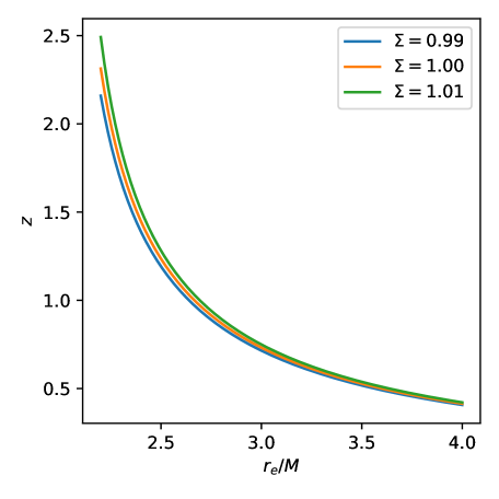
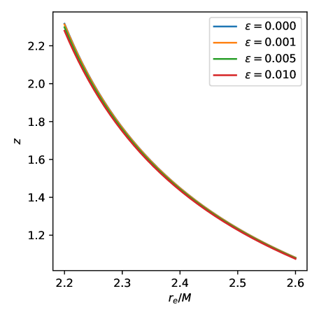
Equation encapsulates the gravitational redshift in the RN metric and is shown in Fig. 1. Notice that in the limit and , Eq. 71 reduces to the well-known redshift formula for the Schwarzschild black hole,
| (72) |
The domain of validity of the event horizon is for , where is the outer (event) horizon. As the function approaches zero, leading to which reflects the infinite redshift at the horizon.
In summary, gravitational redshift encapsulates how the energy of a photon diminishes when traveling from an emitter deeper in a gravitational well to an observer located farther out (or even at spatial infinity). The magnitude of depends on the spacetime geometry, the motion of the emitter (e.g., circular orbits), and the observer’s location and velocity.
IX Ringdown Waveform of the BHGCE
In our study, we restrict attention to static, spherically symmetric black hole geometries. The line element is expressed in its most general form as
| (73) |
with the outer event horizon located at where .
To isolate the effect of the metric on black hole echoes, we perturb the spacetime by a free, massless scalar field , which obeys
| (74) |
Employing the standard separation of variables,
| (75) |
reduces the field equation to a radial and temporal differential equation:
| (76) | |||
where the prime indicates differentiation with respect to ; the coordinate ranges over .
For quasinormal mode (QNM) calculations, the appropriate boundary conditions are imposed: the field is purely ingoing at the horizon () and purely outgoing at infinity. To facilitate this analysis, we map the radial coordinate to the tortoise coordinate defined by
| (77) |
which transforms the wave equation into
| (78) |
with the effective potential given by
| (79) |
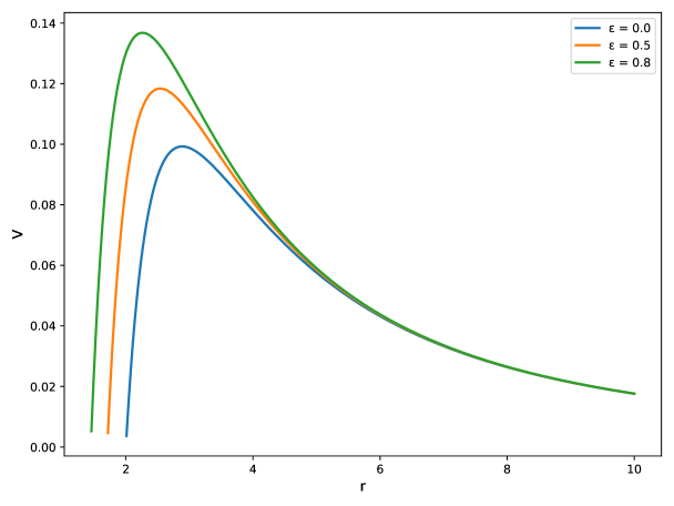
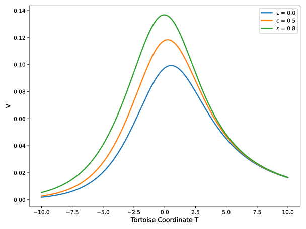
The transformation to reparameterizes the spatial domain (stretching it to ) while preserving the intrinsic structure of the potential, particularly the number of its extrema. In upper Figure 2 we plot the radial profile of the effective potential for three representative values of the deformation parameter, . As increases, the height of the potential barrier grows monotonically, signaling a stronger trapping region for perturbations. Moreover, the location of the peak shifts slightly outward (toward larger ) with larger , indicating that the photon‑sphere radius is pushed to larger radii by the quantum‑vacuum backreaction. Lower Figure 2 shows the same potential plotted against the tortoise coordinate , which logarithmically stretches the near–horizon region. Here, one sees that the barrier becomes both taller and narrower in tortoise space as increases: the uphill “walls” on either side of the peak steepen, reflecting the fact that modes take longer (in coordinate time) to traverse the potential as quantum corrections strengthen.
A brief analysis shows that with a positive slope, . At spatial infinity, assuming an asymptotically flat form (), one obtains and . Consequently, the effective potential must exhibit at least one maximum. In standard black holes such as Schwarzschild or Reissner-Nordström, the single-peak structure precludes echo phenomena, which require a resonant cavity typically associated with at least three extrema—a minimum bounded by two maxima. Notably, for large angular momentum the dominant term behaves as , corresponding to the photon sphere; thus, multiple peaks in are closely linked to the presence of multiple photon spheres, a feature rarely encountered in classical black hole solutions.
To extract the time-domain evolution of as governed by the wave equation, we employ a finite difference approach a method that has proven effective in probing QNMs for both black hole Zhu et al. (2014) and wormhole Liu et al. (2021) geometries.
The temporal and spatial variables are discretized by setting and (with ), and the scalar field and potential are correspondingly denoted by
| (80) |
Under these definitions, the wave equation is approximated by the finite difference equation:
| (81) |
For the initial condition we adopt a Gaussian wave packet:
| (82) |
where defines the center of the packet. We explore two distinct configurations: when the packet is situated outside the double-peaked region of the potential, and when it is located within the well between the peaks. In the latter scenario, as the initial packet is placed nearer to the potential minimum, echo signals become more pronounced and the characteristic echo frequency approximately doubles relative to the exterior configuration.
Boundary conditions are imposed by requiring
| (83) |
with denoting the QNM frequency (distinct from the echo frequency). The update rule is then formulated as
| (84) | |||
To ensure numerical stability, the time step is chosen in compliance with the von Neumann criterion, specifically (see, e.g., Zhu et al. (2014) for further details).
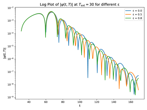
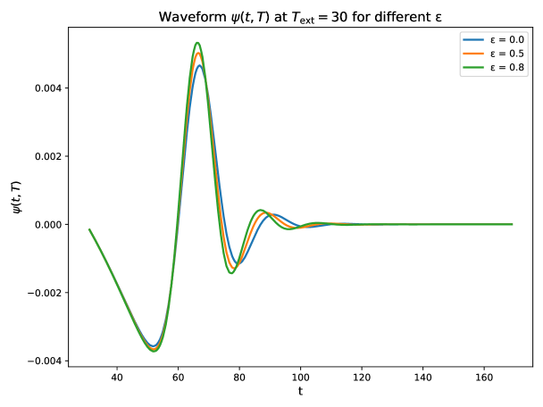
In the lower panel of Figure 3 we display the late‑time ringdown signal (extracted at a fixed observation radius) for the same set of values. With increasing , the oscillation period visibly lengthens, and the envelope decays more slowly. In the upper panel of Figure 3 we plot , which makes the quasi‑periodic oscillations and exponential damping far more transparent: Oscillation Frequency: The spacing between successive peaks in the log‑plot clearly increases with , indicating that the real part of the quasinormal frequency decreases as the GCW deformation grows. Damping Rate: The magnitude of the slope of the peak‑envelope in the plot (i.e. the imaginary part of the mode) diminishes for larger , showing that the ringdown damps more slowly under stronger quantum‑vacuum corrections.
Together, these results demonstrate that both the oscillation frequency and damping rate of the dominant quasinormal mode are sensitive probes of the generalized Compton wavelength parameter.
X Conclusion
In this work, we have investigated the implications of a generalized Compton wavelength framework, embedded in a three-dimensional dynamical quantum vacuum (3D DQV), on a Schwarzschild-like black hole geometry. The introduction of the quantum deformation parameter , which encapsulates backreaction effects due to vacuum energy density fluctuations, modifies the black hole metric in a controlled and theoretically consistent manner. Through analytical methods, we derived explicit corrections to key physical observables and assessed their phenomenological viability.
The black hole shadow analysis in Section III provided an exact expression for the shadow radius, yielding bounds on from EHT observations of Sgr. A* and M87*. These constraints lie within the domain of theoretical consistency and do not exclude significant deviations from general relativity, particularly in the case of Sgr. A*, where negative values corresponding to enhanced gravitational attraction remain observationally viable. The weak deflection angle was computed via two independent methods: the Keeton-Petters post-post-Newtonian expansion and the Gauss-Bonnet topological approach. Both revealed non-trivial corrections scaling with and confirmed that solar system lensing observations restrict to values near zero, with a representative upper bound of consistent with PPN constraints.
Thermodynamically, we found that the Hawking temperature of the modified black hole depends nonlinearly on , with positive deformation reducing the evaporation rate—a feature with potential implications for the fate of primordial black holes. Complementing this, the eikonal quasinormal mode frequencies, computed in Section VII, demonstrated that both the real and imaginary parts of the QNM spectrum are sensitive to and the rescaling factor , suggesting that gravitational wave ringdown observations can serve as a sharp probe of quantum corrections to the metric.
We also derived the gravitational redshift and ringdown waveform in the presence of the GCW-induced deformation. The redshift formula remains analytically tractable and reveals that the modification becomes significant near the horizon. Based on scalar perturbations, the ringdown analysis showed how the effective potential, and consequently the waveform morphology, is altered by varying , offering a potential observational signature in the form of modified echo dynamics.
Taken together, these results highlight the observational richness of the GCW-modified black hole metric. With analytical control over corrections to classical phenomena and consistency with existing data, this framework presents a promising semiclassical window into quantum gravity phenomenology. Further constraints may be extracted through multi-messenger observations involving VLBI shadow imaging, gravitational lensing, and gravitational wave spectroscopy, placing tighter bounds on the deformation parameter and its role in black hole physics.
A natural extension of this work would be exploring the GCW-modified metric’s rotating analogs, particularly examining how the generalized Compton wavelength formalism deforms the Kerr geometry. This would enable the analysis of frame dragging, ergosphere structure, and shadow asymmetry, all key signatures in upcoming high-resolution VLBI measurements. Furthermore, coupling this framework to quantum field dynamics in curved spacetime may yield corrections to greybody factors and emission spectra, deepening the connection between semiclassical gravity and observational signatures.
Acknowledgements.
R. P., A. Ö. and G. L. would like to acknowledge networking support of the COST Action CA21106 - COSMIC WISPers in the Dark Universe: Theory, astrophysics and experiments (CosmicWISPers), the COST Action CA22113 - Fundamental challenges in theoretical physics (THEORY-CHALLENGES), the COST Action CA21136 - Addressing observational tensions in cosmology with systematics and fundamental physics (CosmoVerse), the COST Action CA23130 - Bridging high and low energies in search of quantum gravity (BridgeQG), and the COST Action CA23115 - Relativistic Quantum Information (RQI) funded by COST (European Cooperation in Science and Technology). A. Ö. also thanks to EMU, TUBITAK, ULAKBIM (Turkiye) and SCOAP3 (Switzerland) for their support.References
- Fiscaletti (2025) D. Fiscaletti, “Implications of generalized Compton wavelength in the effects of general relativity,” Theor. Math. Phys. 222, 332–355 (2025).
- Scardigli (1999) Fabio Scardigli, “Generalized uncertainty principle in quantum gravity from micro-black hole gedanken experiment,” Physics Letters B 452, 39–44 (1999).
- Carr et al. (2011) Bernard Carr, Leonardo Modesto, and Isabeau Premont-Schwarz, “Generalized Uncertainty Principle and Self-dual Black Holes,” (2011), arXiv:1107.0708 [gr-qc] .
- Carr (2015) Bernard J. Carr, 1st Karl Schwarzschild Meeting on Gravitational Physics (Springer International Publishing, 2015) pp. 159–167.
- Carr et al. (2015) Bernard Carr, Jonas Mureika, and Piero Nicolini, “Sub-planckian black holes and the generalized uncertainty principle,” Journal of High Energy Physics 2015 (2015), https://doi.org/10.1007/JHEP07(2015)052.
- Lake and Carr (2015) Matthew J. Lake and Bernard Carr, “The compton-schwarzschild correspondence from extended de broglie relations,” Journal of High Energy Physics 2015 (2015), https://doi.org/10.1007/JHEP11(2015)105.
- Carr (2022) B. J. Carr, “The generalized uncertainty principle and higher dimensions: Linking black holes and elementary particles,” Frontiers in Astronomy and Space Sciences 9 (2022), https://doi.org/10.3389/fspas.2022.1008221.
- Bina et al. (2010) A. Bina, S. Jalalzadeh, and A. Moslehi, “Quantum black hole in the generalized uncertainty principle framework,” Physical Review D 81, 023528 (2010).
- Vayenas and Grigoriou (2015) Constantinos G Vayenas and Dimitrios Grigoriou, “Microscopic black hole stabilization via the uncertainty principle,” Journal of Physics: Conference Series 574, 012059 (2015).
- da Silva and Silva (2022) Marcelo Ferreira da Silva and Carlos A. S. Silva, “The Compton/Schwarzschild duality, black hole entropy and quantum information,” (2022), arXiv:2205.09502 [gr-qc] .
- Buoninfante et al. (2020) Luca Buoninfante, Gaetano Lambiase, Giuseppe Gaetano Luciano, and Luciano Petruzziello, “Phenomenology of GUP stars,” Eur. Phys. J. C 80, 853 (2020), arXiv:2001.05825 [gr-qc] .
- Scardigli and Lambiase (2018) Fabio Scardigli and Gaetano Lambiase, “GUP parameter and Lorentz violating terms,” J. Phys. Conf. Ser. 1071, 012019 (2018).
- Scardigli et al. (2017) Fabio Scardigli, Gaetano Lambiase, and Elias Vagenas, “GUP parameter from quantum corrections to the Newtonian potential,” Phys. Lett. B 767, 242–246 (2017), arXiv:1611.01469 [hep-th] .
- Jizba et al. (2023) Petr Jizba, Gaetano Lambiase, Giuseppe Gaetano Luciano, and Luciano Petruzziello, “Coherent states for generalized uncertainty relations as Tsallis probability amplitudes: New route to nonextensive thermostatistics,” Phys. Rev. D 108, 064024 (2023), arXiv:2308.12368 [gr-qc] .
- Lambiase and Scardigli (2022) Gaetano Lambiase and Fabio Scardigli, “Generalized uncertainty principle and asymptotically safe gravity,” Phys. Rev. D 105, 124054 (2022), arXiv:2204.07416 [hep-th] .
- Das et al. (2022) Saurya Das, Mitja Fridman, Gaetano Lambiase, and Elias C. Vagenas, “Baryon asymmetry from the generalized uncertainty principle,” Phys. Lett. B 824, 136841 (2022), arXiv:2107.02077 [gr-qc] .
- Iorio et al. (2020) Alfredo Iorio, Gaetano Lambiase, Pablo Pais, and Fabio Scardigli, “Generalized Uncertainty Principle in three-dimensional gravity and the BTZ black hole,” Phys. Rev. D 101, 105002 (2020), arXiv:1910.09019 [hep-th] .
- Kanazawa et al. (2019) T. Kanazawa, G. Lambiase, G. Vilasi, and A. Yoshioka, “Noncommutative Schwarzschild geometry and generalized uncertainty principle,” Eur. Phys. J. C 79, 95 (2019).
- Lambiase and Scardigli (2018) Gaetano Lambiase and Fabio Scardigli, “Lorentz violation and generalized uncertainty principle,” Phys. Rev. D 97, 075003 (2018), arXiv:1709.00637 [hep-th] .
- Heidari et al. (2023) N. Heidari, H. Hassanabadi, and H. Chen, “Quantum-corrected scattering of a Schwarzschild black hole with GUP effect,” Phys. Lett. B 838, 137707 (2023).
- Hamil et al. (2022) B. Hamil, B. C. Lütfüoğlu, and L. Dahbi, “EUP-corrected thermodynamics of BTZ black hole,” Int. J. Mod. Phys. A 37, 2250130 (2022), arXiv:2203.09394 [gr-qc] .
- Lütfüoğlu et al. (2021) B. C. Lütfüoğlu, B. Hamil, and L. Dahbi, “Thermodynamics of Schwarzschild black hole surrounded by quintessence with generalized uncertainty principle,” Eur. Phys. J. Plus 136, 976 (2021), arXiv:2110.01383 [gr-qc] .
- Hassanabadi et al. (2021) S. Hassanabadi, J. Kříž, W. S. Chung, B. C. Lütfüoğlu, E. Maghsoodi, and H. Hassanabadi, “Thermodynamics of the Schwarzschild and Reissner–Nordström black holes under higher-order generalized uncertainty principle,” Eur. Phys. J. Plus 136, 918 (2021), arXiv:2110.01363 [gr-qc] .
- Lütfüoğlu et al. (2020) B. C. Lütfüoğlu, J. Kříž, P. Sedaghatnia, and H. Hassanabadi, “The generalized Klein-Gordon oscillator in a Cosmic Space-Time with a Space-Like Dislocation and the Aharonov-Bohm Effect,” Eur. Phys. J. Plus 135, 691 (2020), arXiv:2011.02056 [quant-ph] .
- Hamil and Lütfüoğlu (2021) B. Hamil and B. C. Lütfüoğlu, “New Higher-Order Generalized Uncertainty Principle: Applications,” Int. J. Theor. Phys. 60, 2790–2803 (2021), arXiv:2009.13838 [gr-qc] .
- Zakharov (2024) Alexander F. Zakharov, “Shadows near supermassive black holes: From a theoretical concept to GR test,” Int. J. Mod. Phys. D 33, 2340004 (2024), arXiv:2308.01301 [gr-qc] .
- Zakharov (2022) Alexander F. Zakharov, “Constraints on a Tidal Charge of the Supermassive Black Hole in M87* with the EHT Observations in April 2017,” Universe 8, 141 (2022), arXiv:2108.01533 [gr-qc] .
- Zakharov (2014) Alexander F. Zakharov, “Constraints on a charge in the Reissner-Nordström metric for the black hole at the Galactic Center,” Phys. Rev. D 90, 062007 (2014), arXiv:1407.7457 [gr-qc] .
- Khodadi et al. (2020) Mohsen Khodadi, Alireza Allahyari, Sunny Vagnozzi, and David F. Mota, “Black holes with scalar hair in light of the Event Horizon Telescope,” JCAP 09, 026 (2020), arXiv:2005.05992 [gr-qc] .
- Vagnozzi et al. (2023) Sunny Vagnozzi et al., “Horizon-scale tests of gravity theories and fundamental physics from the Event Horizon Telescope image of Sagittarius A,” Class. Quant. Grav. 40, 165007 (2023), arXiv:2205.07787 [gr-qc] .
- Vagnozzi and Visinelli (2019) Sunny Vagnozzi and Luca Visinelli, “Hunting for extra dimensions in the shadow of M87*,” Phys. Rev. D 100, 024020 (2019), arXiv:1905.12421 [gr-qc] .
- Allahyari et al. (2020) Alireza Allahyari, Mohsen Khodadi, Sunny Vagnozzi, and David F. Mota, “Magnetically charged black holes from non-linear electrodynamics and the Event Horizon Telescope,” JCAP 02, 003 (2020), arXiv:1912.08231 [gr-qc] .
- Neves (2020) Juliano C. S. Neves, “Upper bound on the GUP parameter using the black hole shadow,” Eur. Phys. J. C 80, 343 (2020), arXiv:1906.11735 [gr-qc] .
- Tamburini et al. (2022) Fabrizio Tamburini, Fabiano Feleppa, and Bo Thidé, “Constraining the Generalized Uncertainty Principle with the light twisted by rotating black holes and M87*,” Phys. Lett. B 826, 136894 (2022), arXiv:2103.13750 [gr-qc] .
- Anacleto et al. (2021) M. A. Anacleto, J. A. V. Campos, F. A. Brito, and E. Passos, “Quasinormal modes and shadow of a Schwarzschild black hole with GUP,” Annals Phys. 434, 168662 (2021), arXiv:2108.04998 [gr-qc] .
- Karmakar et al. (2023) Ronit Karmakar, Dhruba Jyoti Gogoi, and Umananda Dev Goswami, “Thermodynamics and shadows of GUP-corrected black holes with topological defects in Bumblebee gravity,” Phys. Dark Univ. 41, 101249 (2023), arXiv:2303.00297 [gr-qc] .
- Ong (2023) Yen Chin Ong, “A critique on some aspects of GUP effective metric,” Eur. Phys. J. C 83, 209 (2023), arXiv:2303.10719 [gr-qc] .
- Lambiase et al. (2023) Gaetano Lambiase, Reggie C. Pantig, Dhruba Jyoti Gogoi, and Ali Övgün, “Investigating the connection between generalized uncertainty principle and asymptotically safe gravity in black hole signatures through shadow and quasinormal modes,” Eur. Phys. J. C 83, 679 (2023), arXiv:2304.00183 [gr-qc] .
- Hoshimov et al. (2024) Husanboy Hoshimov, Odil Yunusov, Farruh Atamurotov, Mubasher Jamil, and Ahmadjon Abdujabbarov, “Weak gravitational lensing and shadow of a GUP-modified Schwarzschild black hole in the presence of plasma,” Phys. Dark Univ. 43, 101392 (2024), arXiv:2312.10678 [gr-qc] .
- Chen et al. (2024a) H. Chen, S. H. Dong, E. Maghsoodi, S. Hassanabadi, J. Křiž, S. Zare, and H. Hassanabadi, “Gup-corrected black holes: thermodynamic properties, evaporation time and shadow constraint from EHT observations of M87* and Sgr A*,” Eur. Phys. J. Plus 139, 759 (2024a).
- Lobos and Pantig (2022) Nikko John Leo S. Lobos and Reggie C. Pantig, “Generalized Extended Uncertainty Principle Black Holes: Shadow and Lensing in the Macro- and Microscopic Realms,” MDPI Physics 4, 1318–1330 (2022), arXiv:2208.00618 [gr-qc] .
- Övgün et al. (2024) Ali Övgün, Lemuel John F. Sese, and Reggie C. Pantig, “Constraints via the Event Horizon Telescope for Black Hole Solutions with Dark Matter under the Generalized Uncertainty Principle Minimal Length Scale Effect,” Annalen Phys. 536, 2300390 (2024), arXiv:2309.07442 [gr-qc] .
- Chaudhary et al. (2024) Shahid Chaudhary, Muhammad Danish Sultan, Adnan Malik, Atiq ur Rehman, Ali Övgün, and Ayman A. Ghfar, “Images and stability of black hole with cloud of strings and quintessence in EGUP framework,” Nucl. Phys. B 1006, 116635 (2024).
- Pantig et al. (2025) Reggie C. Pantig, Gaetano Lambiase, Ali Övgün, and Nikko John Leo S. Lobos, “Spacetime-curvature induced uncertainty principle: Linking the large-structure global effects to the local black hole physics,” Physics of the Dark Universe 47, 101817 (2025).
- Fu et al. (2022) Qi-Ming Fu, Shao-Wen Wei, Li Zhao, Yu-Xiao Liu, and Xin Zhang, “Shadow and weak deflection angle of a black hole in nonlocal gravity,” Universe 8, 341 (2022).
- Alloqulov et al. (2025) Mirzabek Alloqulov, Yokubjon Isaqjonov, Sanjar Shaymatov, and Abdul Jawad, “Shadow and gravitational weak lensing around a quantum-corrected black hole surrounded by plasma*,” Chinese Physics C 49, 045104 (2025).
- Pantig (2025) Reggie C. Pantig, “Traces of quantum fuzziness on the black hole shadow and particle deflection in the multi-fractional theory of gravity,” Chin. Phys. C 49, 065102 (2025), arXiv:2410.15106 [gr-qc] .
- Claudel et al. (2001) Clarissa-Marie Claudel, K. S. Virbhadra, and G. F. R. Ellis, “The Geometry of photon surfaces,” J. Math. Phys. 42, 818–838 (2001), arXiv:gr-qc/0005050 .
- Kocherlakota et al. (2021) Prashant Kocherlakota et al. (Event Horizon Telescope), “Constraints on black-hole charges with the 2017 EHT observations of M87*,” Phys. Rev. D 103, 104047 (2021), arXiv:2105.09343 [gr-qc] .
- Epstein and Shapiro (1980) R. Epstein and I. I. Shapiro, “POST POSTNEWTONIAN DEFLECTION OF LIGHT BY THE SUN,” Phys. Rev. D 22, 2947–2949 (1980).
- Will (2014) Clifford M. Will, “The Confrontation between General Relativity and Experiment,” Living Rev. Rel. 17, 4 (2014), arXiv:1403.7377 [gr-qc] .
- Keeton and Petters (2005) Charles R. Keeton and A. O. Petters, “Formalism for testing theories of gravity using lensing by compact objects. I. Static, spherically symmetric case,” Phys. Rev. D 72, 104006 (2005), arXiv:gr-qc/0511019 .
- Ruggiero (2016) Matteo Luca Ruggiero, “Light bending in gravity,” Int. J. Mod. Phys. D 25, 1650073 (2016), arXiv:1601.00588 [gr-qc] .
- Kumaran and Övgün (2022) Yashmitha Kumaran and Ali Övgün, “Deflection Angle and Shadow of the Reissner–Nordström Black Hole with Higher-Order Magnetic Correction in Einstein-Nonlinear-Maxwell Fields,” Symmetry 14, 2054 (2022), arXiv:2210.00468 [gr-qc] .
- Virbhadra and Ellis (2000) K. S. Virbhadra and George F. R. Ellis, “Schwarzschild black hole lensing,” Phys. Rev. D 62, 084003 (2000), arXiv:astro-ph/9904193 .
- Virbhadra et al. (1998) K. S. Virbhadra, D. Narasimha, and S. M. Chitre, “Role of the scalar field in gravitational lensing,” Astron. Astrophys. 337, 1–8 (1998), arXiv:astro-ph/9801174 .
- Virbhadra (2024) K. S. Virbhadra, “Conservation of distortion of gravitationally lensed images,” Phys. Rev. D 109, 124004 (2024), arXiv:2402.17190 [gr-qc] .
- Kudo and Asada (2025) Ryuya Kudo and Hideki Asada, “Correspondence between two gravitational lens equations in a static and spherically symmetric spacetime,” Phys. Rev. D 111, 044014 (2025), arXiv:2407.02046 [gr-qc] .
- Virbhadra (2022) K. S. Virbhadra, “Distortions of images of Schwarzschild lensing,” Phys. Rev. D 106, 064038 (2022), arXiv:2204.01879 [gr-qc] .
- Li et al. (2020) Zonghai Li, Guodong Zhang, and Ali Övgün, “Circular Orbit of a Particle and Weak Gravitational Lensing,” Phys. Rev. D 101, 124058 (2020), arXiv:2006.13047 [gr-qc] .
- Chen et al. (2024b) Ruo-Ting Chen, Shulan Li, Li-Gang Zhu, and Jian-Pin Wu, “Constraints from Solar System tests on a covariant loop quantum black hole,” Phys. Rev. D 109, 024010 (2024b), arXiv:2311.12270 [gr-qc] .
- Fomalont et al. (2009) E. Fomalont, S. Kopeikin, G. Lanyi, and J. Benson, “Progress in measurements of the gravitational bending of radio waves using the vlba,” The Astrophysical Journal 699, 1395–1402 (2009).
- Verlinde (2011) Erik P. Verlinde, “On the Origin of Gravity and the Laws of Newton,” JHEP 04, 029 (2011), arXiv:1001.0785 [hep-th] .
- Misner et al. (1973) Charles W. Misner, K. S. Thorne, and J. A. Wheeler, Gravitation (W. H. Freeman, San Francisco, 1973).
- Nicolini and Spallucci (2010) Piero Nicolini and Euro Spallucci, “Noncommutative geometry inspired wormholes and dirty black holes,” Class. Quant. Grav. 27, 015010 (2010), arXiv:0902.4654 [gr-qc] .
- Cárdenas et al. (2021) Víctor H. Cárdenas, Mohsen Fathi, Marco Olivares, and J. R. Villanueva, “Probing the parameters of a Schwarzschild black hole surrounded by quintessence and cloud of strings through four standard astrophysical tests,” Eur. Phys. J. C 81, 866 (2021), arXiv:2109.08187 [gr-qc] .
- Zhu et al. (2014) Zhiying Zhu, Shao-Jun Zhang, C. E. Pellicer, Bin Wang, and Elcio Abdalla, “Stability of Reissner-Nordström black hole in de Sitter background under charged scalar perturbation,” Phys. Rev. D 90, 044042 (2014), [Addendum: Phys.Rev.D 90, 049904 (2014)], arXiv:1405.4931 [hep-th] .
- Liu et al. (2021) Hang Liu, Peng Liu, Yunqi Liu, Bin Wang, and Jian-Pin Wu, “Echoes from phantom wormholes,” Phys. Rev. D 103, 024006 (2021), arXiv:2007.09078 [gr-qc] .