A transiting rocky super-Earth and a non-transiting sub-Neptune orbiting the M dwarf TOI-771

Abstract

Context. The origin and evolution of the sub-Neptune population is a highly debated topic in the exoplanet community. With the advent of JWST, atmospheric studies can now put unprecedented constraints on the internal composition of this population. In this context, the THIRSTEE project aims to investigate the population properties of sub-Neptunes with a comprehensive and demographic approach, providing a homogeneous sample of precisely characterised sub-Neptunes across stellar spectral types.

Aims. We present here the precise characterisation of the planetary system orbiting one of the THIRSTEE M-dwarf targets, TOI-771 ($d=25$ pc, $V=14.9$ mag), known to host one planet, TOI-771 b, which has been statistically validated using TESS observations.

Methods. We use TESS, SPECULOOS, TRAPPIST and M-Earth photometry together with $31$ high-precision ESPRESSO radial velocities to derive the orbital parameters and investigate the internal composition of TOI-771 b, as well as exploring the presence of additional companions in the system.

Results. We derive precise mass and radius for TOI-771 b, a super-Earth with $R_{\rm b}=1.36\pm 0.10$ R_⊕ and $M_{\rm b}=2.47_{-0.31}^{+0.32}$ M_⊕ orbiting every $2.3$ days around its host star. Its composition is consistent with an Earth-like planet, and it adds up to the rocky population of sub-Neptunes lying below the density gap identified around M dwarfs. With a $\sim 13$% precision in mass, a $\sim 7$% radius precision, and a warm equilibrium temperature of $T_{{\rm eq}}$$=543$ K, TOI-771 b is a particularly interesting target for atmospheric characterisation with JWST, and it is indeed one of the targets under consideration for the Rocky World DDT program. Additionally, we discover the presence of a second, non-transiting planet in the system, TOI-771 c, with a period of $7.61$ days and a minimum mass of $M_{\rm p}$ $\sin{i}=2.87_{-0.38}^{+0.41}$ M_⊕. Even though the inclination is not directly constrained, the planet likely belongs to the temperate sub-Neptune population, with an equilibrium temperature of $\sim 365$ K.

1 Introduction

One of the major discoveries of dedicated exoplanet transit missions like Kepler (Borucki et al., 2010) and TESS (Ricker et al., 2014) has been the identification of the so-called sub-Neptune population. This class of small ($1$ R_⊕ $<$ $R_{\rm p}$ $<4$ R_⊕), close-in ($P<100$ d) planets is absent in our Solar System, but is likely the most abundant in the Milky Way (Batalha et al., 2013; Petigura et al., 2013; Bean et al., 2021; Biazzo et al., 2022). Despite the increasing number of discovered sub-Neptunes, the nature of this population is currently highly debated, both in terms of formation/evolution and composition. In fact, up to now the main observables to constrain their composition have been only mass and radius, but the vast majority of sub-Neptunes lies in a highly degenerate region of the mass-radius diagram, where different theories can explain their bulk densities (Rogers & Seager, 2010). The theories explored till now have mainly followed two strands, namely (1) atmospheric mass-loss processes, based on the atmospheric evolution of rocky cores surrounded by H-He envelopes (e.g. Owen & Wu 2013; Ginzburg et al. 2018; Rogers et al. 2023), and (2) the water-world hypothesis, with a formation beyond the ice line implying a high mass fraction content of volatiles and subsequent inner migration (e.g. Izidoro et al. 2022; Bitsch et al. 2019; Venturini et al. 2020; Dorn & Lichtenberg 2021; Burn et al. 2021).

Both theories can explain the observed properties of the sub-Neptune population (Lissauer et al., 2011; Fabrycky et al., 2014; Weiss & Marcy, 2014; Mulders et al., 2018; Otegi et al., 2020), with one of the most noticeable ones being the dearth of planets in the radius distribution around $1.5$ R_⊕, a feature known as the ‘radius gap’ (Fulton et al., 2017; Fulton & Petigura, 2018; Cloutier et al., 2020; Petigura et al., 2022). Planets below the radius gap are usually termed super-Earths, with bulk compositions consistent with the Earth’s. Planets above the radius gap have lower bulk densities, and they are usually referred to as ‘mini-Neptunes’, even though they can be also called ‘gas dwarfs’ (e.g. Buchhave et al. 2014; Phillips et al. 2021; Rigby et al. 2024) or ‘water worlds’ (e.g. Léger et al. 2004; Luque et al. 2022; Diamond-Lowe et al. 2022; Osborne et al. 2023; Cadieux et al. 2024) depending on the adopted composition and evolution theory.

The launch of JWST provided a unique opportunity to start breaking the degeneracy on the composition of sub-Neptunes, providing further observables and using atmospheric studies to investigate their chemistry and interior structures. JWST recently provided initial, promising results, with the detection of the first molecular features in the atmospheres of a collection of sub-Neptunes (e.g. Madhusudhan et al. 2023; Benneke et al. 2024; Piaulet-Ghorayeb et al. 2024). In this context, planets orbiting M dwarfs are particularly interesting targets, as M dwarfs are the most numerous stars in our Galaxy, and their low mass and radius make the detection of the planetary atmospheres less challenging than for Sun-like stars.

Still, to perform accurate atmospheric retrieval, precise mass measurements ($<20$%) are needed (Batalha et al., 2019), and a large, homogeneous sample of well-characterised sub-Neptunes is essential for demographic studies. The THIRSTEE project represents a significant step in this direction. This international observing program aims to shed light on the sub-Neptune population by providing an enlarged sample of precisely-characterised planets across stellar types, and combining precise and accurate densities with atmospheric characterization and a novel statistical approach (Lacedelli et al., 2024). We report here the characterization of the planetary system orbiting one of the THIRSTEE M-dwarf targets, TOI-771. We analysed TESS (Sect. 2) and ground-based photometry together with ESPRESSO radial velocities (RVs) collected under the THIRSTEE program (Sect. 3) to derive stellar parameters (Sect. 4) and precise mass, radius, and orbital configuration of the planetary system orbiting TOI-771 (Sect. 5), identifying a second, non-transiting candidate. Finally, we discuss our results and the characterization of the TOI-771 system in the context of the THIRSTEE project and of the atmospheric characterisation picture (Sect. 6).

2 TESS photometry

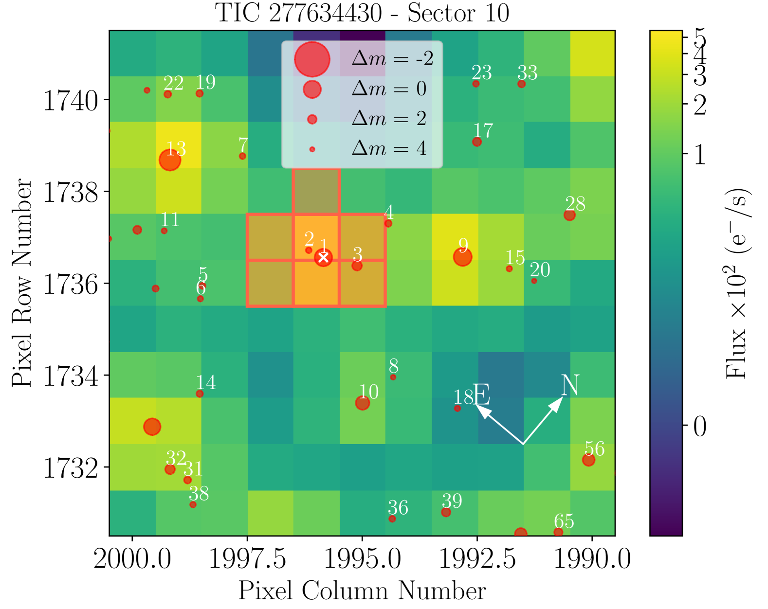
Figure 1: Sector 10 TPF image of TOI-771 computed with tpfplotter. The red squares mark the TESS aperture used for the photometric extraction. Red circles show Gaia DR3 (Gaia Collaboration et al., 2023) stars with magnitude contrast up to $\Delta m=4$. Star 1 corresponds to TOI-771. The SPOC pipeline accounts for dilution due to stars 2 ($G=16.56$ mag) and 3 ($G=15.07$ mag) using the crowding metric and subtracting the corresponding median flux level percentage (Guerrero et al., 2021). The TPFs images of the remaining sectors are reported in Appendix A.

TESS observed TOI-771 for a total of seven sectors, summarised in Table 1. The two-minute cadence light curves were reduced using the Science Processing Operations Center (SPOC) pipeline (Jenkins et al., 2016; Jenkins, 2020). The SPOC pipeline identified a $2.33$-day period candidate (TOI-771.01), which was vetted and statistically validated as TOI-771 b by (Mistry et al., 2024) using the validation tool TRICERATOPS (Giacalone & Dressing, 2020; Giacalone et al., 2021), together with ground-based photometric and high-resolution imaging follow-up observations from the TESS Follow-up Observing Program (TFOP; Collins 2019).

For our analysis we downloaded the two-minute cadence Pre-search Data Conditioning Simple Aperture Photometry (PDCSAP, Smith et al., 2012; Stumpe et al., 2012, 2014) light curves from the Mikulski Archive for Space Telescopes (MAST). The target field of view and the photometric apertures selected for each sector and used by the SPOC pipeline for the light curve extraction are shown in the target pixel file (TPF) images computed with tpfplotter (Aller et al., 2020) in Figs. 1 and 18.

For our photometric analysis, we first removed from the PDCSAP light curves all points flagged as ‘bad quality’ (DQUALITY>0), and we performed a $3\sigma$ clipping to remove outliers, after masking the in-transit points according to the Mistry et al. (2024) planetary parameters. The resulting light curves are presented in Figs. 20 and  21.

Table 1: Summary of TESS observations for TOI-771.

Sectors	Dates
10, 11, 12	March 26-June 19, 2019
37, 38	April 2-May 26, 2021
64, 65	April 6-June 2, 2023

3 Ground-based follow-up observations

TOI-771 b has been statistically validated by Mistry et al. (2024) using ground-based follow-up observations, including high-resolution imaging data and photometric transit observations scheduled using the TESS Transit Finder tool (Jensen, 2013) as part of the TFOP program. All the TFOP light curves initially employed in Mistry et al. (2024) (their Table 3) as input for the statistical validation of the planet are available on the EXOFOP-TESS webpage. Here, we included all those light curves for the first time in the global modelling (Sect. 5.3). In addition, we collected four additional transits as part of the SPECULOOS consortium. We detail below all the ground-based photometric and RV observations that we employed in this work to characterise TOI-771 b.

3.1 M-Earth-South photometry

We observed one transit window of TOI-771 b as part of TFOP with the eight 0.4 m M-Earth-South telescopes (Irwin et al., 2007) located at Cerro Tololo Inter-American Observatory, Chile. Observations were taken on February 2, 2020 using the RG715 filter. Data analysis and extraction were performed through the custom pipelines outlined in Irwin et al. (2007). We used a circular photometric aperture of $5\aas@@fstack{\prime\prime}0$, which excluded the nearest neighbour in the Gaia DR3 catalogue (Gaia DR3 5229384714548082944).

3.2 TRAPPIST-South photometry

We observed two transit windows of TOI-771 b as part of TFOP with the TRAnsiting Planets and PlanetesImals Small Telescope (TRAPPIST) South 0.6 m telescope (Jehin et al., 2011; Gillon et al., 2011) located at ESO La Silla Observatory, Chile. The first transit was observed on January 29, 2022 in the I+z band, while the second one on February 2, 2022 in the Sloan $z^{\prime}$ band. As part of the TRAPPIST consortium, we collected an additional transit on March 19, 2022 in the I+z band. Data calibration and photometric extraction were performed using either AstroImageJ or the dedicated prose pipeline outlined in Garcia et al. (2022). We used circular photometric apertures of $4\aas@@fstack{\prime\prime}5$, $5\aas@@fstack{\prime\prime}0$, and $4\aas@@fstack{\prime\prime}6$ respectively, to exclude the nearest neighbour star Gaia DR3 5229384714548082944.

3.3 SPECULOOS-South

We observed two transit windows of TOI-771-b as part of TFOP with the SPECULOOS Southern Observatory (SSO, Jehin et al. 2018) located at the ESO Paranal Observatory, Chile. Both transits were observed in the Sloan $g^{\prime}$ band, one with the 1-m SSO-Io telescope on February 5, 2022, and one with the 1-m SSO-Europa telescope, on April 2, 2022. As part of the SPECULOOS consortium, we collected three additional transits, one on March 19, 2022 with the SSO-Europa telescope in the Sloan-$g^{\prime}$ band, and two during the same night on April 20, 2024, one with the SSO-Io telescope and one with the SSO-Callisto telescope, both in the Sloan-$i^{\prime}$ band. Data calibration and extraction was performed with a specific pipeline, reported in Sebastian et al. (2020). We used circular photometric apertures of $3\aas@@fstack{\prime\prime}3$ for the SSO-Io and $3\aas@@fstack{\prime\prime}6$ for SSO-Europa TFOP observations, to exclude the nearest neighbour star Gaia DR3 5229384714548082944. For the additional transits, circular photometric apertures of $2\aas@@fstack{\prime\prime}2$, $5\aas@@fstack{\prime\prime}1$, and $3\aas@@fstack{\prime\prime}0$ were used for the Europa, Io and Callisto telescopes, respectively.

3.4 Long-term photometric monitoring

We recovered the All-Sky Automated Survey for Supernovae (ASAS-SN; Shappee et al. 2014, Kochanek et al. 2017) photometric V and g long-term light curves of TOI-771 from the ASAS-SN portal (Hart et al., 2023). The star was observed in the V filter between 2014 and 2018, for a total time span of $\sim 1538$ days, with a median cadence of $\sim 3$ days. The median magnitude is $V=14.25$ mag, the median photometric uncertainty $\sigma_{V}$ is $0.009$ mag, and the root mean square (RMS) is $0.027$ mag. In the g filter, observations span from 2017 to 2024, for a total of $\sim 2363$ days, with a median cadence of $\sim 1$ d. The median magnitude, uncertainty and RSM are $g=14.77$ mag, $\sigma_{g}=0.010$ mag and RMS $=0.039$ mag. The time series are plotted in Fig. 2. The photometric precision and cadence of the ASAS-SN light curves are not suited to detect the transiting planet, but they were employed to study the stellar activity and investigate the stellar rotational period (see Sect. 4.2). For this analysis, we filtered the light curves selecting only the good-quality flagged observations (QUALITY=G), and rejecting the outliers by applying a $5\sigma$ clipping, as in (Hart et al., 2023).

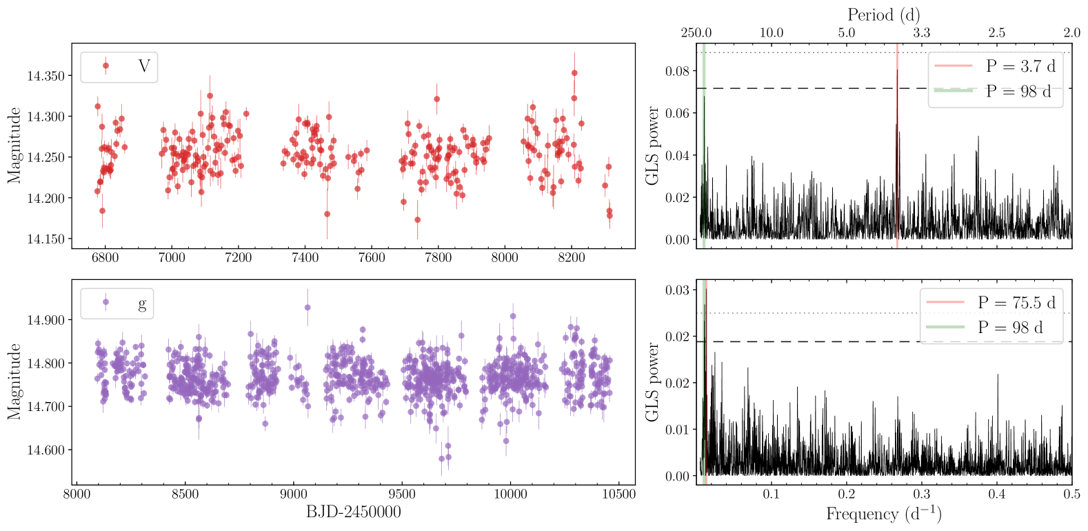
Figure 2: ASAS-SN V- and g photometry of TOI-771. The GLS periodogram of each light curve is shown in the right panel, with the $10$% and $1$% FAP levels marked with an horizontal dashed and dotted line, respectively. The vertical red line highlights the most significant peak, while the vertical green line shows the periodicity at $\sim 98$ d.

3.5 ESPRESSO spectroscopic observations

We collected $31$ high-resolution spectra of TOI-771 with the Echelle SPectrograph for Rocky Exoplanets and Stable Spectroscopic Observations (ESPRESSO, Pepe et al. 2021) installed at the ESO Very Large Telescope telescope array at Paranal Observatory, Chile. The star was selected as part of THIRSTEE RV follow-up (Lacedelli et al., 2024), and it was observed within the 112.25F2.001 program (PI: E. Palle). The observations span between December 6, 2023, and March 9, 2024, covering a total baseline of $\sim 94$ days. We employed the ESPRESSO’s single Unit Telescope (1UT) set-up, using the high-resolution (HR) mode ($1$ arcsec fibre, $R\sim 140000$) with the $2\times 1$ detector binning (HR21), covering the spectral range $\sim 380-780$ nm. For background subtraction, we selected the observing configuration with fibre B placed on the sky. Spectra were gathered with an exposure time of $1800$ seconds, resulting in a median signal-to-noise ratio (S/N) of $17$ at $550$ nm. Data were reduced using ESPRESSO’s data reduction pipeline (DRS), version 3.0.0. Following the methodology of Lacedelli et al. (2024), seeking for an homogeneous analysis of the whole THIRSTEE sample, we extracted the RV values using the template-matching SERVAL algorithm (Zechmeister et al., 2018). The resulting RV dataset, listed in Table 5, has an RMS of $3.99$ m s^-1 and a median internal uncertainty of $0.65$ m s^-1.

4 The star

Table 2: Stellar properties of TOI-771.

[t] TOI-771 TIC 277634430 Gaia DR3 5229384714547758720 2MASS J10562716-7259054 Parameter Value Source RA (J2000; hh:mm:ss.ss) 10:56:27.34 A Dec (J2000; dd:mm:ss.ss) $-$72:59:06.66 A $\mu_{\alpha}$ (mas yr^-1) $39.300\pm 0.017$ A $\mu_{\delta}$ (mas yr^-1) $-76.417\pm 0.015$ A Parallax (mas) $39.4467\pm 0.0136$ A Distance (pc) $25.325\pm 0.008$ B $\gamma$ (km s^-1) $-5.90\pm 1.02$ A U (km s^-1) $4.56\pm 0.42$ F^a V (km s^-1) $9.86\pm 0.91$ F^a W (km s^-1) $-4.82\pm 0.21$ F^a TESS (mag) $12.087\pm 0.007$ C G (mag) $13.343\pm 0.003$ A G_BP (mag) $14.877\pm 0.004$ A G_RP (mag) $12.141\pm 0.004$ A B (mag) $16.768\pm 0.162$ C V (mag) $14.888\pm 0.080$ C J (mag) $10.507\pm 0.023$ D H (mag) $9.955\pm 0.022$ D K (mag) $9.664\pm 0.021$ D W1 (mag) $9.479\pm 0.023$ E W2 (mag) $9.303\pm 0.020$ E W3 (mag) $9.173\pm 0.024$ E W4 (mag) $8.885\pm 0.216$ E $T_{{\rm eff}}$ (K) $3370\pm 100$ F log g  (cgs) $4.80\pm 0.07$ F, Spectroscopic log g  (cgs) $5.05\pm 0.14$ F, Bolometric $[$Fe/H$]$ (dex) $-0.13\pm 0.07$ F $\log{\rm R}^{\prime}_{\rm HK}$ $-6.36\pm 0.06$ F $P_{\rm rot}$ (d) $98_{-5}^{+10}$ F $R_{\star}$ (R_⊙) $0.232^{+0.017}_{-0.023}$ F $M_{\star}$ (M_⊙) $0.220^{+0.030}_{-0.035}$ F $L_{\star}$ ($L_{\odot}$) $0.00626^{+0.00015}_{-0.00053}$ F Spectral type M3 F A) Gaia DR3 (Gaia Collaboration et al., 2023). B) Bailer-Jones et al. (2021). C) TESS Input Catalogue Version 8 (TICv8, Stassun et al. 2018). D) Two Micron All Sky Survey (2MASS, Cutri et al. 2003). E) Wide-field Infrared Survey Explorer (AllWISE; Cutri et al., 2021). F) This work.

4.1 Stellar parameters

To obtain homogeneous parameters for the THIRSTEE sample, we used the same methodology as in Lacedelli et al. (2024) to derive the stellar parameters of TOI-771. We applied the SteParSyn (Tabernero et al., 2022) code to the ESPRESSO spectra, combining the BT-Settl stellar atmospheric models (Allard et al., 2012), and atomic and molecular data from the Vienna atomic line database (VALD3, see Ryabchikova et al., 2015) with the Turbospectrum-generated (Plez, 2012) grid of synthetic spectra. We employed an optimised set of Fe i and Ti i lines, as well as various TiO molecular bands, for M-type stars, following (Marfil et al., 2021). We obtained the following parameters: $T_{\rm eff}$ $=$ 3370 $\pm$ 18 K, $\log{g}$ $=$ 4.80 $\pm$ 0.07 dex, and [Fe/H] $=$ $-0.13$ $\pm$ 0.07 dex. The first set of error bars refers only to the internal errors, and to estimate a more realistic uncertainty on $T_{{\rm eff}}$(see also Tayar et al. 2022), we added a systematic component to the errors, following Marfil et al. (2021), for a final temperature value and uncertainties of $T_{\rm eff}$ $=$ 3370 $\pm$ 100 K. All our derived parameters, listed in Table 2, are consistent within $1\sigma$ with Mistry et al. (2024).

To derive the stellar luminosity, mass and radius, we first computed the photometric spectral energy distribution (SED) of TOI-771 (Fig. 3) using the publicly available broad-band photometry from the American Association of Variable Star Observers Photometric All-Sky Survey (APASS, Henden & Munari, 2014), the Sloan Digital Sky Survey (SDSS instead York et al., 2000), the Gaia DR3 archive (Gaia Collaboration et al., 2016, 2023), 2MASS (Skrutskie et al., 2006), and the Wide-field Infrared Survey Explorer archive (WISE, Wright et al., 2010). We used the zero points listed in the Virtual Observatory SED Analyzer tool (VOSA, Bayo et al., 2008) to convert the observed magnitudes into fluxes, and the Gaia DR3 trigonometric parallax to transform from observed to absolute fluxes. We then integrated the observed SED to obtain the stellar bolometric luminosity $L_{\star}=0.00626^{+0.00015}_{-0.00053}$ L_⊙, which we employed together with our derived $T_{{\rm eff}}$ to compute the stellar radius ($R_{\star}=0.232^{+0.017}_{-0.022}$ R_⊙) using the Stefan-Boltzmann law. We then used the mass-radius relation of Schweitzer et al. (2019) to derive the stellar mass $M_{\star}=0.221^{+0.030}_{-0.035}$ M_⊙. As a consistency check, we compared the surface gravity obtained using our mass and radius values (log g$=5.05\pm 0.14$ dex), with our derived spectroscopic value (log $g=4.80\pm 0.07$ dex), confirming that they are consistent within 1.5 $\sigma$.

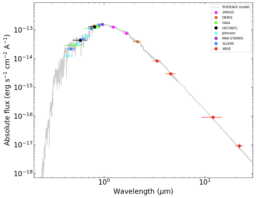
Figure 3: SED of TOI-771. The grey line shows the BT-Settl model (which uses the PHOENIX atmospheric code) assuming $T_{{\rm eff}}$ $=3300$ K, log g $=5.0$ dex, and solar metallicity.

Finally, we performed a kinematic analysis of TOI-771 to assess its position in the Galactic framework. Starting from Gaia DR3 positions, proper motions, parallax, and systemic RV (see Table 2), we computed the galactic heliocentric space velocities in the directions of the Galactic centre, Galactic rotation, and north Galactic pole, obtaining $U=44.05\pm 0.31$ km s^-1, $V=-44.44\pm 0.29$ km s^-1, and $W=-0.18\pm 0.29$ km s^-1, respectively. Based on these values, and adopting the probabilistic framework of Bensby et al. (2014), we infer that TOI-771 kinematically belongs to the thin-disk population.

4.2 Activity indices and rotational period

To identify the stellar rotational period, we first analysed the ASAS-SN photometry. The generalised Lomb-Scargle (GLS, Zechmeister & Kürster 2009) periodogram of the ASAS-SN $V$ and $g$ light curves show the most significant periodicity at $3.7$ d and $75.5$ d, respectively (see Fig. 2). However, the $3.7$ d periodicity is not identified in the TESS periodogram, neither in the PDCSAP nor in the SAP light curves, and it is likely to be related to the light curve cadence ($\sim 3$ d). Additionally, both ASAS-SN time series show a second periodicity around $\sim 98$ d, especially significant in the g filter. We searched for this long-period signal in the TESS SAP light curve, but we could not identify it, probably due to the clustering of the sectors, favouring shorter periods (see Appendix B and Fig. 19).

This long-term periodicity is also identified in the spectroscopic time series. Indeed, we analysed various spectral activity indicators of the ESPRESSO dataset, including the SERVAL absorption line indicators (Na i doublet ($\lambda\lambda 589.0$ nm, $589.6$ nm), H$\alpha$ ($\lambda 656.2$ nm), and $S$-index (Ca ii H&K lines, $\lambda\lambda 396.8470$ nm, $393.3664$ nm), as derived from the ACTIN2 code (Gomes da Silva et al., 2018, 2021)), the RV chromatic index (CRX) and the differential line width (dLW; see Zechmeister et al. 2018 and Jeffers et al. 2022 for more details). Moreover, we included in the analysis the ESPRESSO DRS (Baranne et al., 1996; Pepe et al., 2002) activity indexes, namely the bisector span (BIS) (Queloz et al., 2001), the full-width-half-maximum (FWHM), and the contrast (Contr) of the cross-correlation function (CCF), which was computed using the M3 ESPRESSO DRS mask.

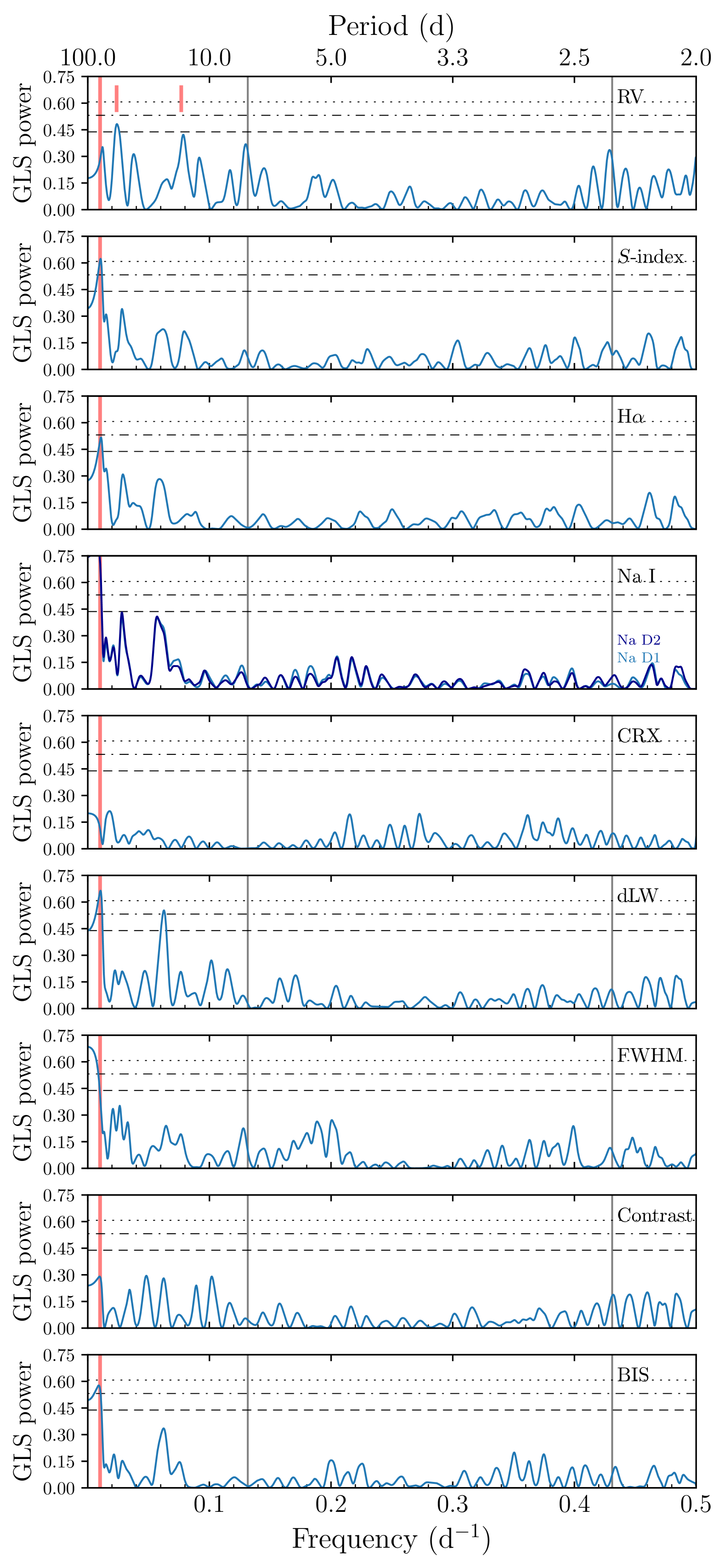
Figure 4: GLS periodogram of the TOI-771 ESPRESSO RVs and activity indicators. The vertical red line marks the possible stellar rotational period at $\sim 98$ days. The vertical red ticks in the RV periodogram mark the peaks at $\sim 42$ d and $\sim 13$ d, which are related to each other, and to the $98$-d signal (see Fig. 5). The vertical grey lines show the periods of TOI-771 b ($2.33$ d), and of the second planet candidate TOI-771 c ($\sim 7.6$ d). The $10\%$, $1$%, and 0.1% FAP levels are drawn with dashed, dash-dotted, and dotted horizontal lines, respectively.

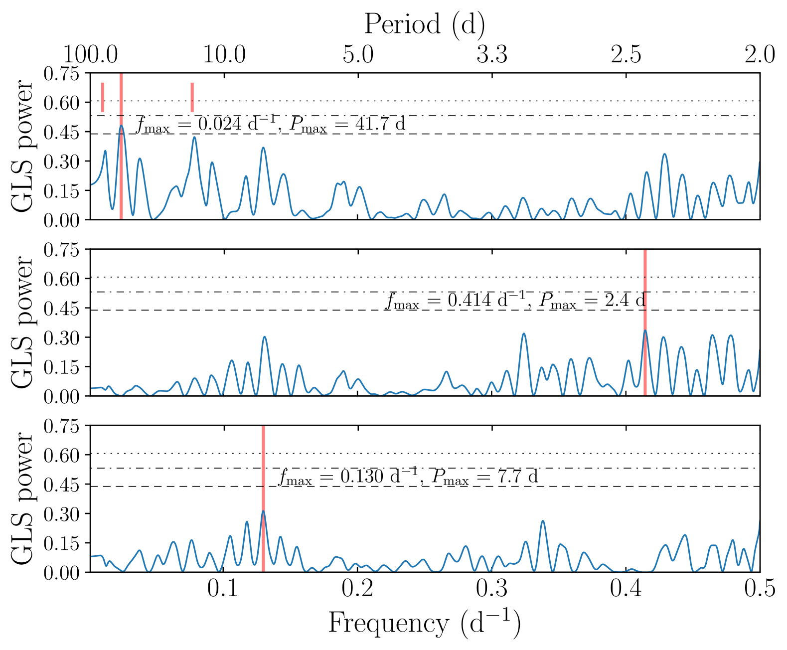
Figure 5: Iterative GLS periodogram of the TOI-771 ESPRESSO RVs. The sinusoidal model corresponding to the best frequency is subtracted at each iteration, starting from top to bottom. The vertical red line marks most significant peak in each iteration, and the corresponding frequency and period are reported. The vertical red ticks in the first panel mark the peaks at $\sim 98$ d and $\sim 13$ d, which are related to each other and to the $42$-d signal. All three peaks disappear after the first iteration. The $10\%$, $1$%, and 0.1% FAP levels are drawn with dashed, dash-dotted, and dotted horizontal lines, respectively.

We show the GLS periodograms of the ESPRESSO RVs and activity indexes in Fig. 4. The most significant peak in the RVs periodogram is identified at $\sim 42$ d, and we associate it to an alias of the long-term signal at $\sim 98$ d. In fact, when removing the $42$ d signal from the periodogram, the $\sim 98$ d peak also vanishes (see Fig. 5). The $98$-d signal is also present with high significance in various activity indicators, especially in the $S$-index, H$\alpha$, dLW, and BIS (Fig. 4).

To search for additional periodicities in the RV time series, we performed an iterative frequency search on the GLS periodogram, subtracting at each iteration the sinusoidal model associated to the most significant frequency. As Fig. 5 shows, our search identified the frequencies $f_{\rm 1}=0.024$ d^-1 ($P_{\rm 1}=41.8$ d), $f_{\rm 2}=0.415$ d^-1 ($P_{\rm 2}=2.4$ d, corresponding to TOI-771 b), and $f_{\rm 3}=0.130$ d^-1 ($P_{\rm 3}=7.7$ d), even though with low significance. The first signal at $42$ d is related not only to the $98$-d peak, but also to the one at $\sim 13$ d, since they both disappear in the periodogram when subtracting the $42$-d signal (Fig. 5).

The presence of these three peaks, with the long-term periodicity recovered as a broad peak around $100$ d, TOI-771 b’ signal at $\sim 2.3$ d, and an additional signal at $\sim 7.7$ d, is further confirmed from our analysis using the $\ell_{1}$ periodogram (Hara et al., 2017). Due to the intrinsic algorithm construction, fewer peaks related to aliases are identified in the $\ell_{1}$ periodogram (Fig. 6). Given the presence of a similar periodicity (around $90-100$ d) in the ASAS-SN photometry, as well as in various spectroscopic activity indicators, we identify this long-term signal as the rotational period of the star, and we fitted the RVs time series together with the S-index (see Sec. 5.3) to recover the stellar rotational period, obtaining P_rot$=98_{-5}^{+10}$ d. Such a slow rotation is consistent with the low activity level of the star ($\log{\rm R}^{\prime}_{\rm HK}$ $=-6.361\pm 0.056$, computed from the median $S$-index, assuming $B-V=1.88$ and applying (Suárez Mascareño et al., 2016) relations) in the optical regime (Suárez Mascareño et al., 2016; Astudillo-Defru et al., 2017). However, considering the $94$-days time span of the current ESPRESSO dataset, RV observations spanning a longer baseline will be necessary to definitively confirm the nature and periodicity of this signal, which is only broadly constrained by the current analysis.

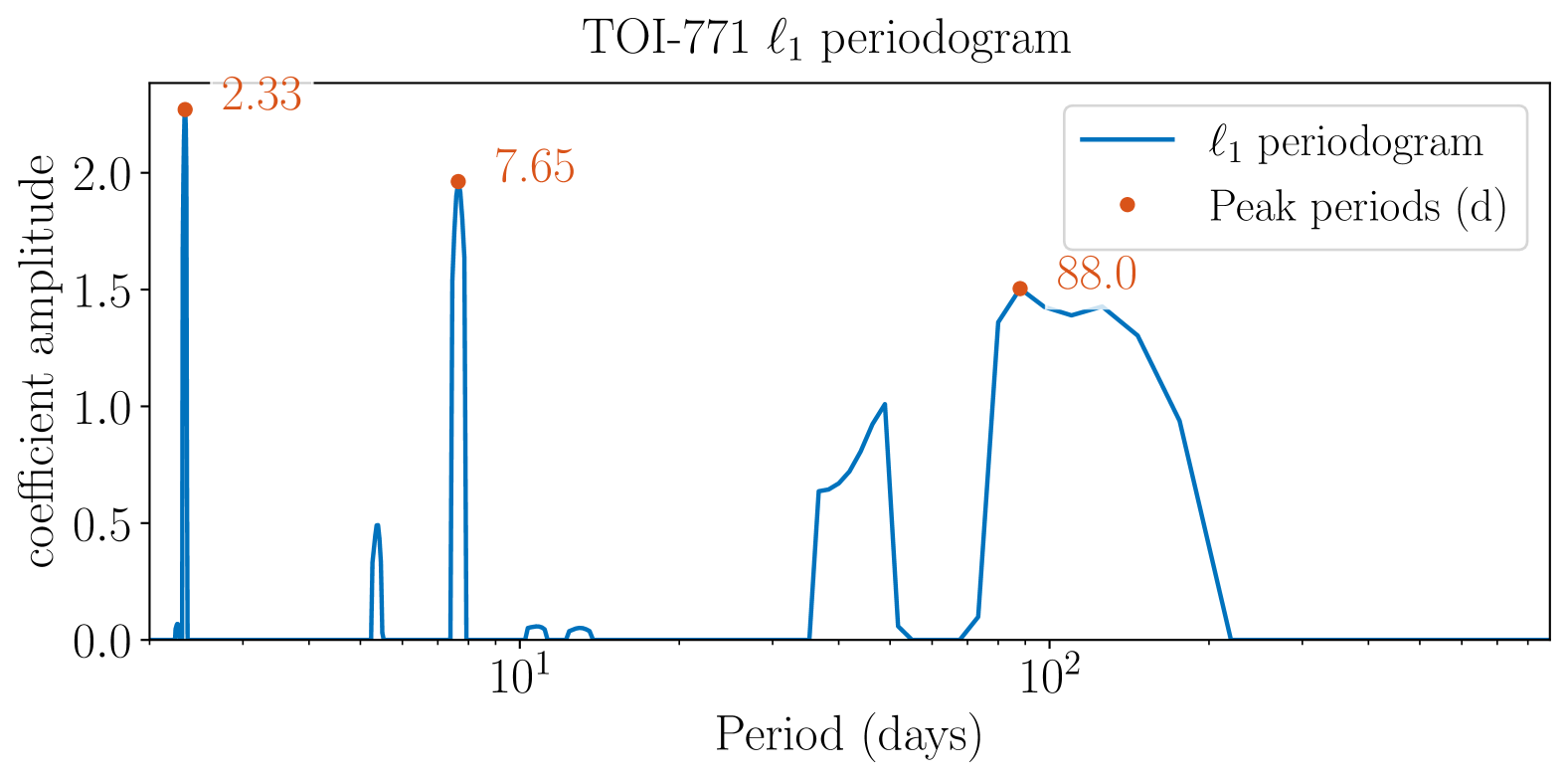
Figure 6: $\ell_{1}$ periodogram of TOI-771 ESPRESSO RVs. The frequency grid is computed from 0 to 1 cycle per day. The time-span of the observations is $\sim 94$ days. Significant peaks (with $\Delta\ln\mathcal{Z}>10$, $\mathcal{Z}$ being the Bayesian evidence) are highlighted with orange dots.

5 Data analysis and results

5.1 Photometric fit

We performed an initial fit of the TESS light curves only, to recover the transit of TOI-771 b using PyORBIT (Malavolta et al., 2016, 2018), a versatile Python framework which allows for the modelling of light curves, RVs, transit time variations, and stellar activity. We employed the PyDE + emcee (Foreman-Mackey et al., 2013) PyORBIT set-up, using the same convergence criteria of (Lacedelli et al., 2022). We employed $2n_{\mathrm{dim}}$ walkers, being $n_{\mathrm{dim}}$ the dimensionality of the model, and we ran the chains for $250000$ iterations, discarding the first $30000$ steps as burn-in and adopting a thinning factor of $100$. We used batman (Kreidberg, 2015) as implemented in PyORBIT to fit the mid-transit time ($T_{0}$), the period ($P$), the stellar radius ratio ($R_{\mathrm{p}}/$$R_{\star}$), the impact parameter ($b$), and the stellar density ($\rho_{\star}$), using our derived parameters (Table 2) as a Gaussian prior. We adopted a quadratic limb-darkening (LD) law with Kipping (2013) parametrisation ($q_{1}$, $q_{2}$), using PyLDTk (Husser et al., 2013; Parviainen & Aigrain, 2015) to estimate the initial values of the coefficients, which we imposed as a Gaussian priors adopting a custom $0.1$ uncertainty. Finally, we included a jitter term to account for additional, uncorrelated noise. For all the fitted parameters, we adopted uniform priors, unless specified otherwise.

We performed an initial fit including a Gaussian Process (GP) regression model with a Matérn-3/2 kernel. The resulting model is shown in Fig. 20. Given the low activity level of the star, and the absence of strong correlated noise, we then tested a second model on pre-detrended TESS light curves. We detrended the light curves using WOTAN (Hippke et al., 2019), adopting a biweight time-windowed slider with a $1$ d window, and masking the in-transit points to preserve the transit shape. The resulting light curves and model are shown in Fig. 21. A comparison between the planetary parameters derived from both fits provided consistent results. Therefore, to reduce the computational time, for the joint analysis in Sect. 5.3 we adopted the pre-detrended light curves without including a GP model.

5.2 Radial velocity fit

According to our frequency analysis, the signal identified in the RV time series at $7.6$ d is unlikely to be related to stellar activity, as none of the activity indicators shows significant peaks at such period. Therefore, we hypothesised the presence of an additional planetary candidate, and we tested its presence by comparing the Bayesian evidence of a one-planet model versus a two-planet model. We computed the Bayesian evidence using the dynamical nested-sampling (NS) algorithm dynesty (Skilling, 2004, 2006; Speagle, 2020) as implemented in PyORBIT. In both fits, we assumed for each planet a wide uniform prior on the RV semi-amplitude ($K\in[0.01$-$100$] m s^-1), exploring it in logarithmic space, and a half-Gaussian zero-mean prior (Van Eylen et al., 2019) on the eccentricity $e$, adopting the ($\sqrt{e}\sin{\omega}$, $\sqrt{e}\cos{\omega}$) parametrisation of Eastman et al. (2013), where $\omega$ is the argument of periastron. For TOI-771 b, we assumed Gaussian priors on $T_{0}$ and $P$ from (Mistry et al., 2024), and in the two-planet fit we allowed the period of the second candidate to span between $3$ and $40$ days, i.e. with the upper limit smaller than the alias of the stellar rotational period. We also included a systemic RV offset, and a jitter term to account for extra stellar and instrument noise. We investigated both the cases with and without stellar activity, to test the robustness of the planetary detection. When including stellar activity, we modelled it using a GP regression with a quasi-periodic kernel (Grunblatt et al., 2015). We assumed as GP hyper-parameters the stellar rotation period (P_rot), the characteristics decay timescale ($P_{\mathrm{dec}}$), the coherence scale (w), and the GP amplitude ($A$). We ran the NS fits assuming 1000 live points and a sampling efficiency of 0.3.
Table 3 reports the obtained Bayesian evidences of the models, as well as the semi-amplitudes, and the period of the second candidate. Overall, the models including the GP modelling are strongly favoured with respect to the case with no stellar activity, with a difference in the logarithmic Bayes factor $2\,\Delta\ln\mathcal{Z}>7$ (Kass & Raftery, 1995). Moreover, both in the case with and without the GP modelling, the two-planet model is favoured with respect to the one-planet model. Therefore, also considering our frequency analysis in Sect. 4.2, we decided to adopt the two-planet model with the GP as the final one, and we identify the $7.6$ d periodicity with a second planet in the system, TOI-771 c. As Table 3 shows, the semi-amplitude of TOI-771 b is consistent among all fits, but modelling the stellar activity and the additional signal including a second planet improves significantly the precision on $K_{\rm b}$.

Table 3: Comparison between the one-planet (1P) and two-planet (2P) models parameters, with and without GP modelling.

Model	$\Delta\ln\mathcal{Z}$	$K_{\mathrm{b}}$ (m s-1)	$K_{\mathrm{c}}$ (m s-1)	$P_{\mathrm{c}}$ (d)
1P	$-98.9\pm 0.1$	$2.7_{-1.5}^{+1.0}$	-	-
2P	$-97.4\pm 0.2$	$2.99_{-0.75}^{+0.71}$	$3.02_{-1.10}^{+0.71}$	$7.64_{-0.09}^{+0.07}$
1P + GP	$-93.9\pm 0.1$	$3.11_{-0.59}^{+0.52}$	-	-
2P + GP	$-89.1\pm 0.2$	$3.32\pm 0.32$	$2.55_{-0.56}^{+0.33}$	$7.60_{-0.03}^{+0.03}$

As a further test, to evaluate the robustness of the obtained semi-amplitude of TOI-771 b, we also tried a less flexible approach, modelling the stellar activity with a sinusoid instead of using GPs. We included in the model the two planetary signals plus a third Keplerian with a circular orbit, and we explored the periodicities at $\sim 98$ d and its alias at $\sim 42$ d in two different runs, using wide, uniform priors around the test period. In the first case, we obtained a consistent semi-amplitude of $K_{\mathrm{b}}=3.49\pm 0.31$ m s^-1, recovering a period of $102_{-7}^{+10}$ d for the sinusoidal signal. When fitting the activity period alias (deriving $P_{\rm rot}=42_{-4}^{+2}$ d), the fit struggled to reach convergence, and we only obtained a partial (yet consistent) detection for planet b ($K_{\mathrm{b}}=2.33_{-1.0}^{+0.68}$ m s^-1). Moreover, the difference in the Bayes factor between the two models ($2\,\Delta\ln\mathcal{Z}=19.9$) strongly favours the $\sim 98$ d period for the stellar activity modelling. In all cases, the semi-amplitude of TOI-771 b is consistent within $1\sigma$ between the models, showing the robustness of the result.

5.3 Joint photometric and RV modelling

We analysed all the TESS and ground-based light curves together with the spectroscopic data using PyORBIT, adopting the two-planet model as described in Sect. 5.2 and the photometric parameters as described in Sect. 5.1. In the joint fit, we also included the $S$-index time series as a proxy of the stellar activity, due to the significant signal detected around the expected rotational period of the star (Sect. 4.2), and we modelled it together with the RVs, to better inform the GP (Osborn et al., 2021; Langellier et al., 2021; Rajpaul et al., 2021; Barragán et al., 2023). We assumed P_rot, $P_{\mathrm{dec}}$, and w as common GP hyper-parameters for the two covariance matrices, while we independently fitted the amplitude of each covariance matrix. For the light curve modelling, we fitted the LD coefficients independently for each filter, using the PyLDTk (Husser et al., 2013; Parviainen & Aigrain, 2015) estimates as initial values with a $0.1$ uncertainty as Gaussian priors. We adopted the TESS model described in Sect. 5.1, while for each ground-based dataset we included a quadratic term in the modelling to account for potential systematics, and an additional jitter term. Table 4 reports our best-fitting parameters. Figures 7 and 8 show the transit models from TESS and ground-based photometry, respectively. The phase-folded RVs and the global RV model are displayed in Figs. 9 and 10.

We derived precise planetary parameters for TOI-771 b, a super-Earth with $R_{\rm b}=1.36\pm 0.10$ R_⊕, $M_{\rm b}=2.47_{-0.31}^{+0.32}$ M_⊕ (from $K_{\rm b}=3.29\pm 0.28$ m s^-1), and a bulk density of $\rho_{\rm b}=5.4\pm 1.4$ g cm^-3. The planet orbits with a period of $2.32$ d, implying an equilibrium temperatures of $T_{{\rm eq}}$ $=543_{-34}^{+28}$ K . Additionally, we recovered a second periodic signal in the RVs, which we identify as the non-transiting planet TOI-771 c (see also Sect. 6.2), with a minimum mass of $M_{\rm c}=2.87_{-0.38}^{+0.41}$ M_⊕  (from $K_{\rm c}=2.58_{-0.25}^{+0.27}$ m s^-1) and a period of $7.61\pm 0.03$ d.

We also recover a broad value for the stellar rotational period at $P_{\rm rot}=98_{-5}^{+10}$ days from our GP joint modelling of the RVs and $S$-index (see Fig. 10), a periodicity that we also tentatively recovered in the ASAS-SN photometry (Sect. 4.2). However, given the short baseline of the RV observations, a longer time-span is needed to definitely confirm the value of the stellar rotational period, which showed a couple of aliases in the RV dataset.

No additional signals have been identified in the ESPRESSO residuals after the joint fit (Fig. 10). As a further confirmation, we performed an additional fit including a third Keplerian signal, from which we obtained consistent results for planets b and c, while the parameters of the additional signal did not converge. We therefore adopt the results described in this section as our final results, as no additional planets can be identified in the current RV and photometric (see Sect. 5.4) datasets.

Finally, given the presence of an additional planet in the system, we investigated the presence of possible transit timing variations (TTVs) of TOI-771 b due to the gravitational interaction among the two planets. We performed a photometric fit of both TESS and ground-based data with PyORBIT as described in Section 5.1, but leaving each T₀ as a free parameter. We then compared the observed transit times with the predicted ones derived from the linear ephemeris (T₀ and $P$ as in Table 4) to evaluate the TTVs presence. We could not identify any significant TTV trend (see Fig. 22), with all transit times being consistent with the linear ephemeris within $2\sigma$. This is not surprising, giving that the period commensurability of the two planets is not close to any first-order mean motion resonance (see also Sect. 6.3), when the TTV signal is expected to be enhanced (Agol et al., 2005; Holman & Murray, 2005).

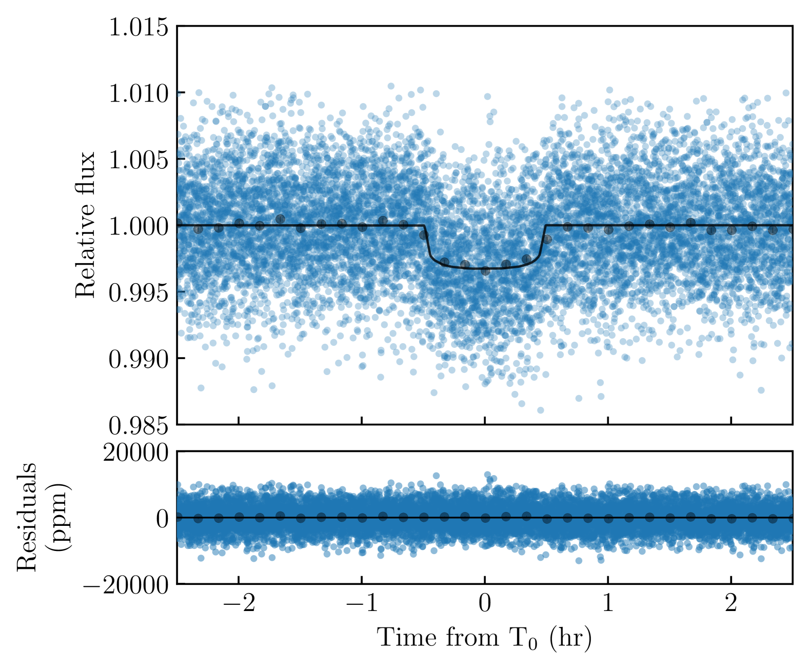
Figure 7: Phase-folded TESS photometry of TOI-771 b. The solid black line shows the best-fitting model. Data binned over $10$ min are shown as black dots. Residuals are displayed in the bottom panel.

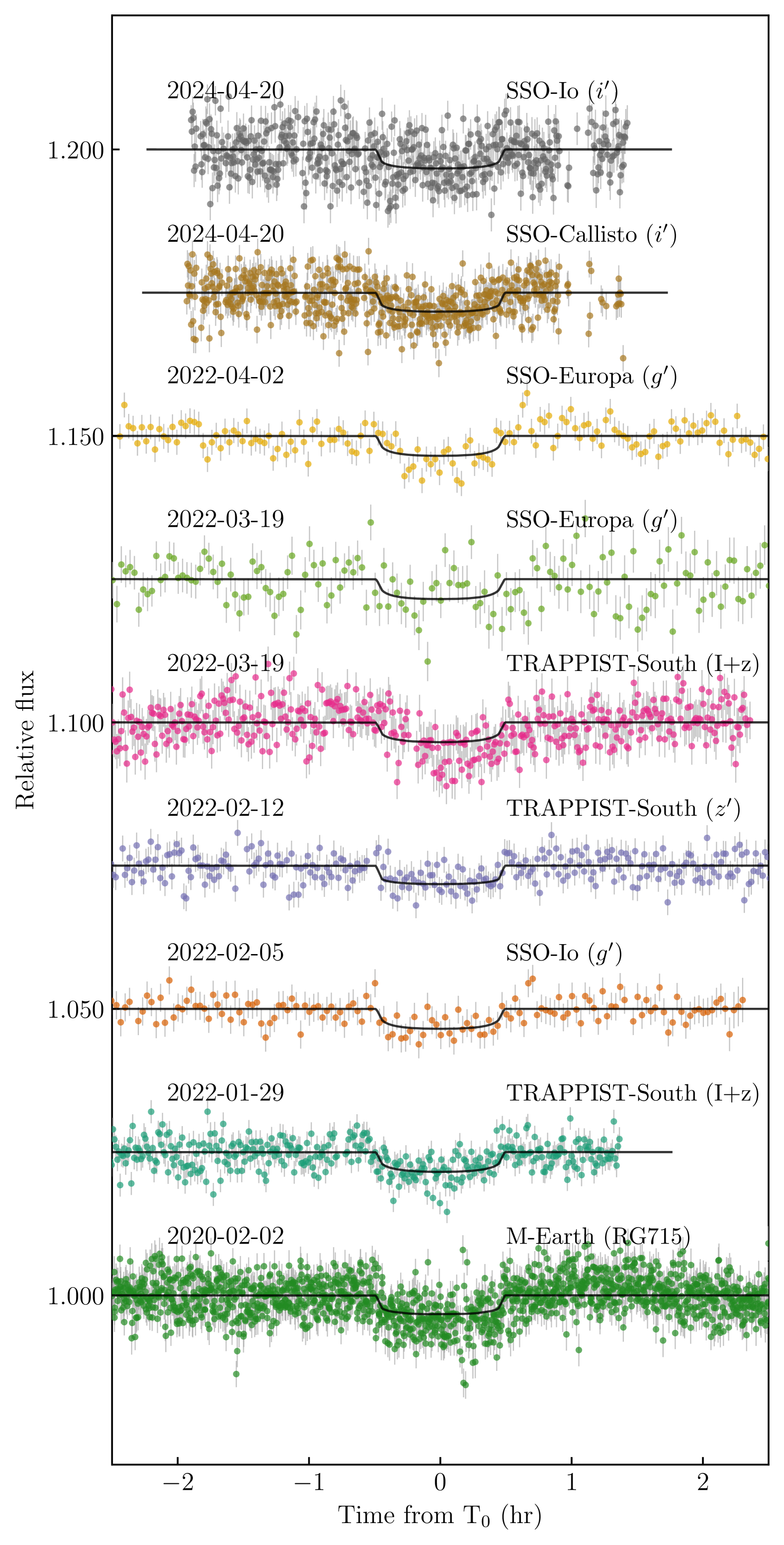
Figure 8: Ground-based photometric light curves of TOI-771 b. The solid black line shows the best-fitting model.

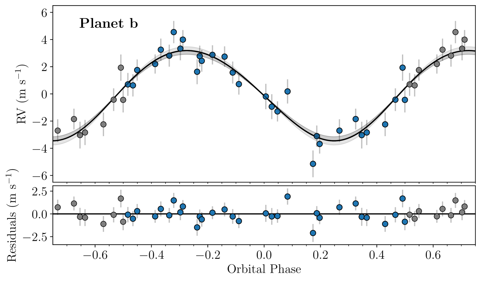
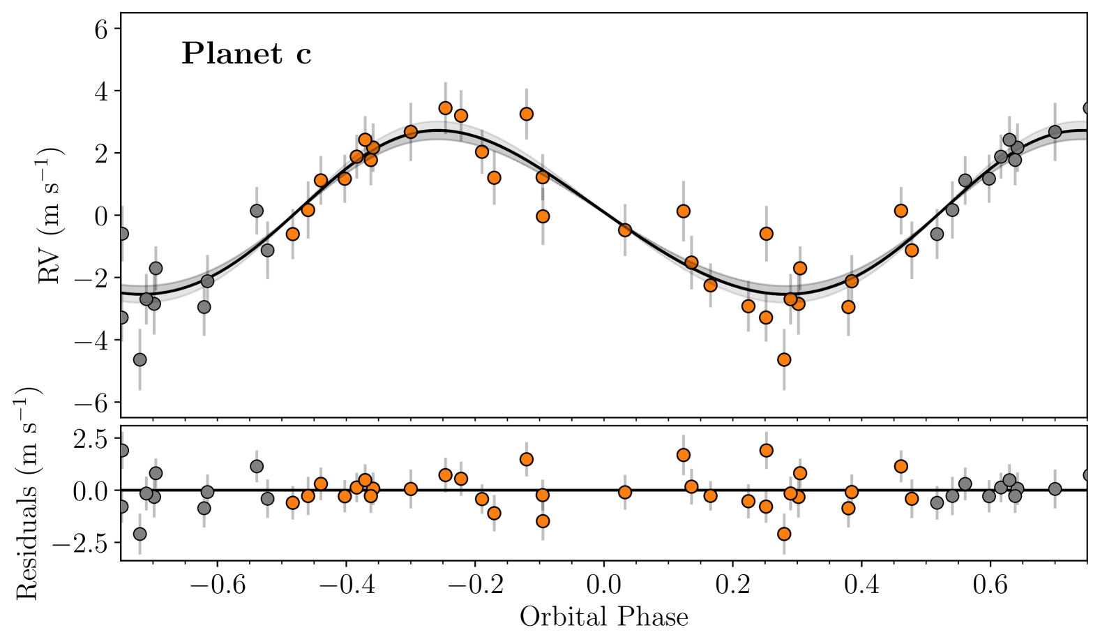
Figure 9: Phase-folded RVs of TOI-771 b and c and global RV model from the joint analysis. In the phase-folded plots, the coloured points shows the ESPRESSO data (with over-phased points in gray), and the solid black line shows the best-fitting model, with the $\pm 1\sigma$ region displayed as a shaded area. Residuals are shown in the bottom panel. The jitter term has been added in quadrature to each error bar.

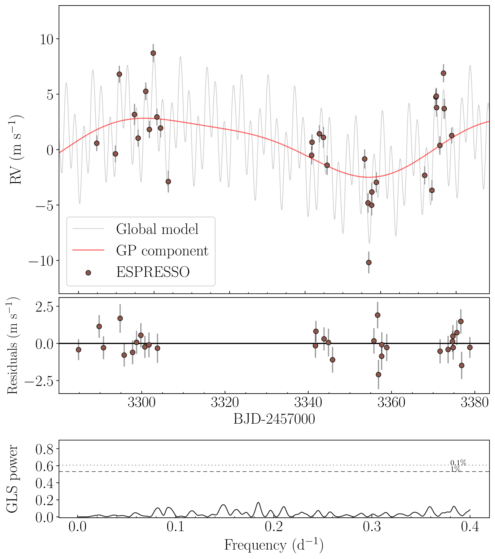
Figure 10: TOI-771 RV model from the joint fit. The solid grey line shows the best-fit global model, while the red solid line refers to GP component. Residuals are shown in the central panel. The jitter term has been added in quadrature to each error bar. The GLS periodogram of the residuals is shown in the bottom panel. The $1$% and $0.1$% FAP levels are marked with a dashed and dotted horizontal line, respectively. No significant signals are identified in the periodogram.

Table 4: Best-fitting parameters of the TOI-771 system.

[t] Planetary parameters TOI-771 b TOI-771 c $P$ (d) $2.3260155_{-0.0000009}^{+0.0000010}$ $7.61\pm 0.03$ $T_{0}$ (TBJD)^a $1572.4191_{-0.0003}^{+0.0003}$ $1573.8\pm 2.5$ $a/$$R_{\star}$ $18.9\pm 1.1$ $42\pm 2$ $a$ (AU) $0.0208_{-0.0010}^{+0.0009}$ $0.046\pm 0.002$ $R_{\mathrm{p}}/$$R_{\star}$ $0.05369\pm 0.0008$ - $R_{\rm p}$ (R_⊕) $1.36\pm 0.10$ - $b$ $0.22_{-0.16}^{+0.18}$ - $i$ (deg) $89.3\pm 0.5$ - $T_{14}$ (h) $0.96_{-0.05}^{+0.04}$ - $e$ $0.055_{-0.036}^{+0.047}$ $0.065_{-0.045}^{+0.062}$ $\omega$ (deg) $-130_{-66}^{+38}$ $-82_{-84}^{+88}$ $K$ (m s^-1) $3.29\pm 0.28$ $2.58_{-0.25}^{+0.27}$ $M_{\rm p}$ (M_⊕) $2.47_{-0.31}^{+0.32}$ - $M_{\rm p}$ $\sin{i}$ (M_⊕) - $2.87_{-0.38}^{+0.41}$ $\rho_{\rm p}$ (g cm^-3) $5.4\pm 1.4$ - $\rho/\rho_{\oplus,s}^{b}$ $0.84\pm 0.22$ - $S_{\rm p}$ ($S_{\oplus}$) $14_{-3}^{+4}$ $3.0_{-0.7}^{+0.6}$ $T_{\rm eq}^{c}$ (K) $543_{-34}^{+28}$ $365_{-19}^{+22}$ $g_{\rm p}^{d}$ (m s^-2) $13\pm 2$ - Common parameters $\rho_{\star}$ ($\rho_{\odot}$) $16.8_{-2.7}^{+3.0}$ $u_{1,\mathrm{TESS}}$ $0.17\pm 0.08$ $u_{2,\mathrm{TESS}}$ $0.40_{-0.08}^{+0.10}$ $u_{1,\mathrm{RG715}}$ $0.25\pm 0.10$ $u_{2,\mathrm{RG715}}$ $0.31\pm 0.10$ $u_{1,\mathrm{g^{\prime}}}$ $0.26\pm 0.09$ $u_{2,\mathrm{g^{\prime}}}$ $0.54_{-0.10}^{+0.09}$ $u_{1,z^{\prime}}$ $0.19\pm 0.09$ $u_{2,z^{\prime}}$ $0.27\pm 0.10$ $u_{1,i^{\prime}}$ $0.23\pm 0.10$ $u_{2,i^{\prime}}$ $0.36\pm 0.09$ $u_{1,\mathrm{I+z}}$ $0.33\pm 0.10$ $u_{2,\mathrm{I+z}}$ $0.37\pm 0.10$ $\sigma_{\rm j,ESPRESSO}^{\rm e}$ (m s^-1) $0.72_{-0.24}^{+0.27}$ $\gamma_{\rm ESPRESSO}^{\rm f}$ (m s^-1) $-4.6\pm 4.2$ GP hyper-parameters P_rot (d) $98_{-5}^{+10}$ $P_{\rm dec}$ (m s^-1) $771_{-288}^{+169}$ $w$ (m s^-1) $0.95_{-0.07}^{+0.04}$ $A^{\rm g}_{\rm RV}$ (m s^-1) $4.9_{-1.6}^{+2.9}$ $A^{\rm g}_{\rm S-index}$ (m s^-1) $0.68_{-0.18}^{+0.34}$

5.4 Photometric planet searches and detection limits

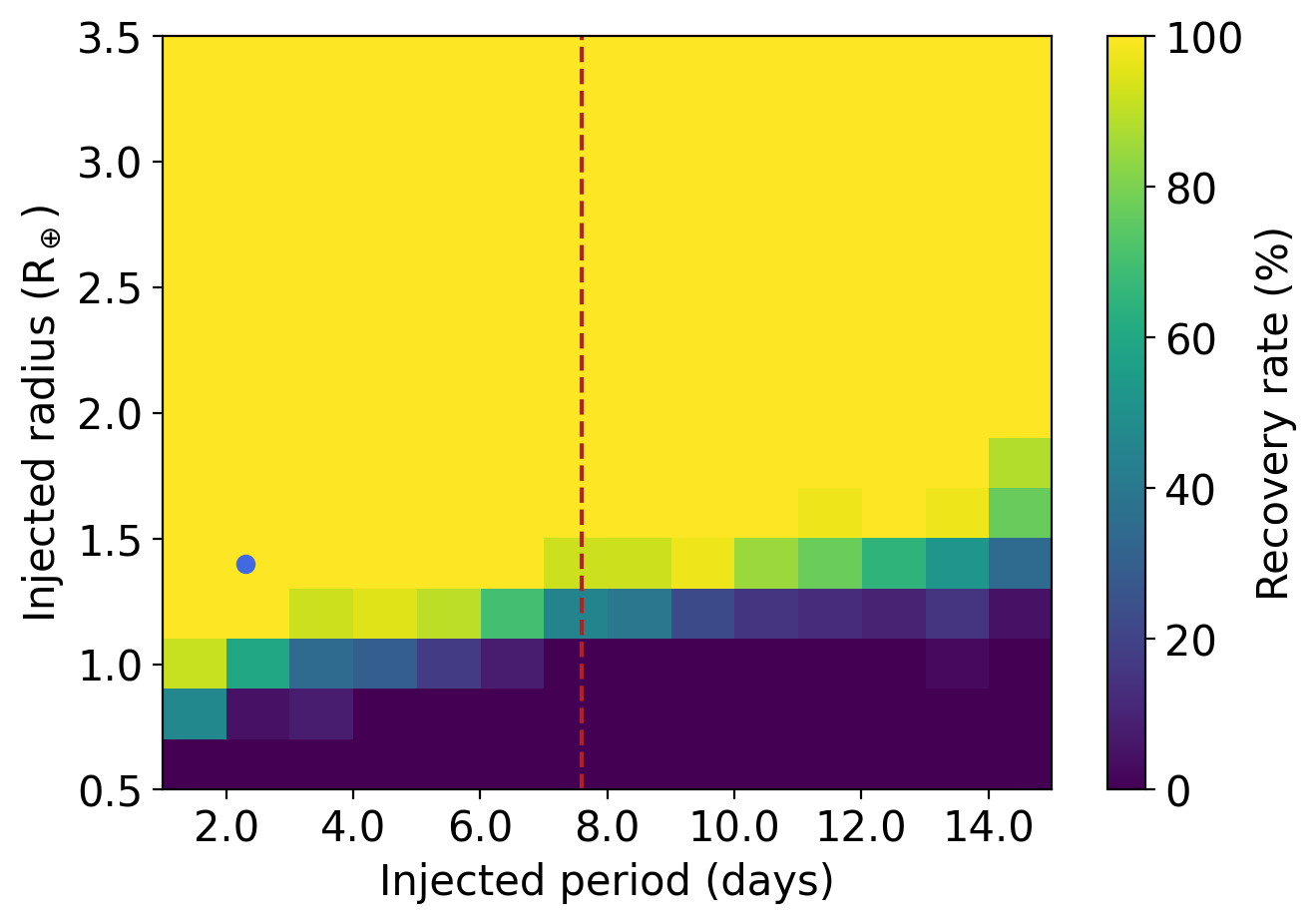
Figure 11: Detectability map of TOI-771. The injection-and-recovery experiment was conducted to establish the detection limits using the TESS data. The blue dot marks the position of TOI-771 b, while the dotted red line indicates the 7.6 d period of TOI-771 c as inferred from the RV fit. We explored 9000 different scenarios, where each pixel evaluates $\sim$45 of them. Larger recovery rates are presented in yellow and green colors, while lower recovery rates are shown in blue and darker hues.

As described in Sect.5, we found the presence of an extra planet in our RV dataset, with a period of $\sim 7.6$ d. There is no alert associated with this orbital period coming from TESS, which might hint at the non-transiting nature of this planet. Still, some transiting planets may remain undetected due to the high detection thresholds employed by official search pipelines, such as SPOC and Quick-Look Pipeline (QLP, Huang et al. 2020), which effectively render low S/N ratio planets undetectable (see, e.g., Delrez et al., 2022; Peterson et al., 2023; Gillon et al., 2024). Hence, to confirm or rule out the transiting nature of this candidate, we carefully examined the available TESS data using the SHERLOCK pipeline (Pozuelos et al., 2020; Demory et al., 2020). This pipeline is an open-source package that relies on six modules to (1) automatically acquire the data from an online database; (2) search for transiting planetary candidates; (3) perform a vetting of the detected signals; (4) conduct a statistical validation of the vetted signals; (5) refine the ephemerides by employing a Bayesian inference framework to model the transit light curves; and (6) find the upcoming transit windows observable from ground-based observatories. See Pozuelos et al. (2023) for recent applications and different searching strategies, and Dévora-Pajares et al. (2024) for further details of the most updated pipeline version.

In our first trial, we allowed SHERLOCK to search for signals with orbital periods ranging from 0.5 to 20 d. After our first execution, we found a strong signal with a period of 2.32 d, which corresponds to the known planet TOI-771 b. During the subsequent runs, we found some additional weaker signals, all attributable to non-corrected noise or spurious results. We also conducted a dedicated search around the expected period of the planet TOI-771 c, with a period grid ranging from 7.3 to 7.9 d; however, we did not find any hint of a transiting signal in this range.

The lack of a signal corresponding to the orbital period of TOI-771 c does not necessarily confirm the non-transiting nature of this planet, as it could remain below our detection limit. To test this hypothesis, we conducted an injection-and-recovery experiment that allows us to build a detectability map based on the TESS data. To this end, we employed the MATRIX package (Dévora-Pajares & Pozuelos, 2022). MATRIX generates a sample of synthetic planets by combining a range of orbital periods, planetary radii, and orbital phases, it injects them into the TESS light curve, and it executes a searching module mimicking the SHERLOCK algorithm. In particular, we generated 9000 scenarios by combining a grid of 30 periods (from 1 to 15 d), 30 radii (from 0.5 to 3.5 $R_{\oplus}$), and 10 different epochs. Our results are displayed in Fig. 11, where we find that any transiting planet larger than 1.6 R_⊕ in our range of studied periods would have been detected using the current dataset, yielding recovery rates higher than 80$\%$. Hence, this result allows us to confirm the non-existence of any transiting planet with $R_{\rm p}$ $\geq$1.6 R_⊕ with orbital periods shorter than 15 d in the TOI-771 system. Considering the semi-amplitude derived from our RV fit (Sect. 5.2), and assuming the same inclination of TOI-771 b ($i=89.3\pm 0.5$, see Sect. 5.3), we derived a minimum mass of $M_{\rm p}\sin{i}=2.9\pm 0.4$ M_⊕ for TOI-771 c. Using spright, a Python Bayesian tool to compute the radius-density-mass relations for small planets (Parviainen et al., 2024), we obtained a radius distribution with $R_{\rm p}$ lying between $1.3$ R_⊕ and $4.1$ R_⊕ (95% limits), with the most probable value being $R_{\rm p}$ $=1.46$ R_⊕ (see also Sect. 6.2). Our detectability map allows us to rule out most of the potential sizes for TOI-771 c, and hence, the planet is most likely not transiting, even though there is a small probability of non-detection in the lower limit case of $R_{\rm p}$ $=1.3$ R_⊕, where we have a recovery rate of $\sim$50$\leavevmode\nobreak\ \%$. In addition, our detectability map also allowed us to confirm that Earth and sub-Earth-sized planets are extremely challenging, if not impossible, to detect using TESS photometry on such systems.

6 Discussion

6.1 TOI-771 b planetary properties

Following the THIRSTEE goal of identifying population patterns within sub-Neptunes, we compared the position of TOI-771 b in the mass-radius diagram with respect to the well-characterised population of planets with $R_{\rm p}$ $<4$ R_⊕ orbiting M dwarfs (Fig. 12). Very similarly to TOI-406 c, the first M-dwarf planet characterised within THIRSTEE (Lacedelli et al., 2024), the density of TOI-771 b is slightly lower than Earth’s, but still consistent with a rocky composition. Considering its equilibrium temperature of $\sim 543$ K, higher than the runaway greenhouse limit (Turbet et al., 2020), a supercritical steam atmosphere (that could be a consequence of magma ocean-hydrogen interactions Kite & Barnett 2020; Rogers et al. 2024) could explain TOI-771 b’s density, if water is present in a few percentages of mass fraction. Moreover, if water is present, the planet interior could be lighter also because of water solubility (Dorn & Lichtenberg, 2021; Luo et al., 2024).

In the attempt to quantify the water mass fraction of the planet, we performed interior modelling using ExoMDN (Baumeister & Tosi, 2023), a machine-learning algorithm which uses the observed planetary radius $R_{\rm p}$, mass $M_{\rm p}$, and equilibrium temperature $T_{{\rm eq}}$ to infer the internal planet composition assuming a four fixed-layers model (iron core, silicate mantle, water and high-pressure ice layer, H/He envelope). Figure 13 shows the thickness (i.e. the radius fraction) and the mass fraction of the interior layers of TOI-771 b, using as input our derived $M_{\rm p}$, $R_{\rm p}$ and $T_{{\rm eq}}$ (Table 4). As expected, when assuming the ExoMDN model properties, TOI-771 b has a prominent planetary iron core, taking up to $63$% of the planet size and $72$% of its mass. For the other layers, the model predicts a possibly considerable mantle ($19$% in mass fraction), a relatively small water layer ($\sim 6$% in mass fraction), and a negligible amount of gas.

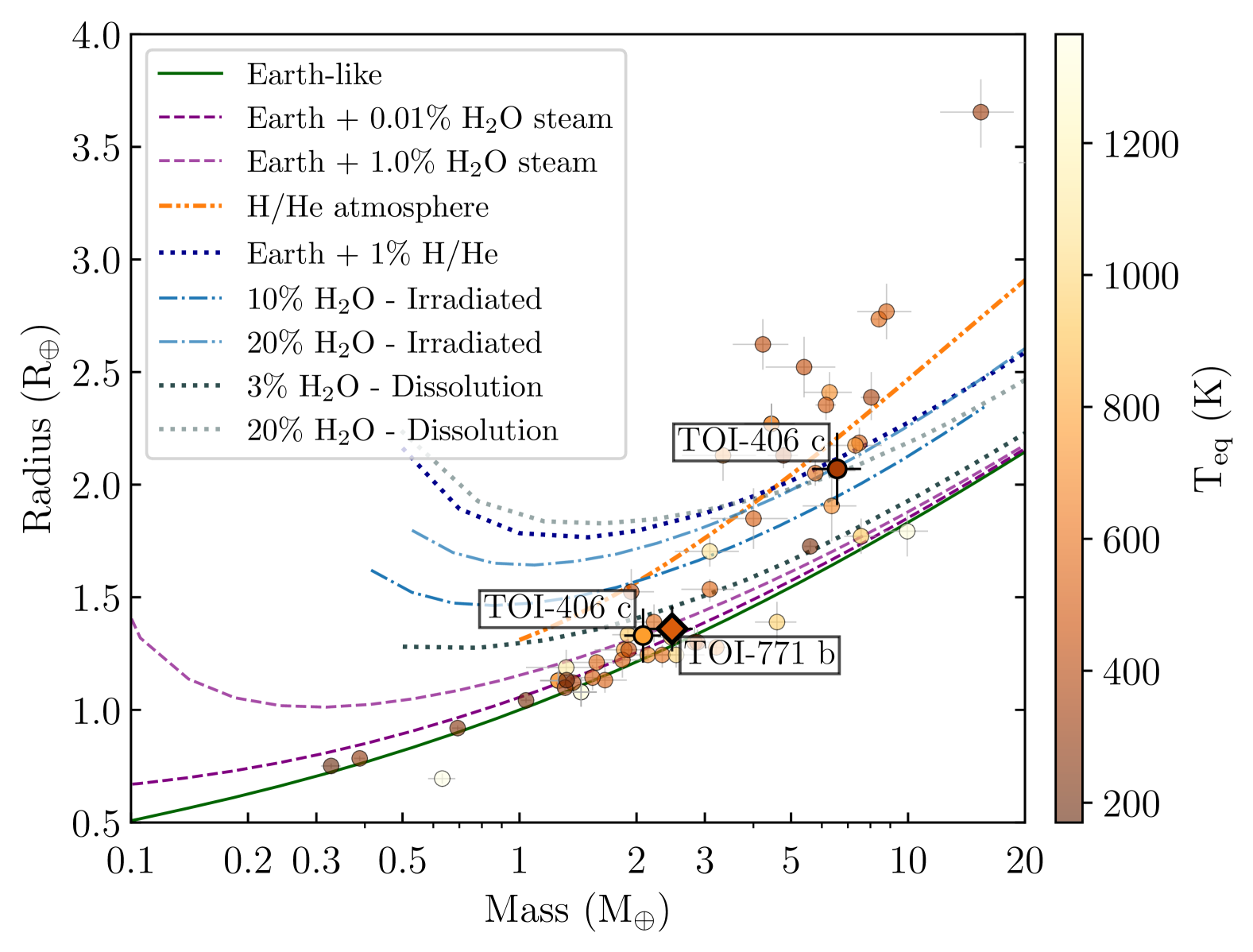
Figure 12: Mass-radius diagram for well-characterised M-dwarf exoplanets with $R_{\rm p}$$<4$ R_⊕. The orange diamond marks the position of TOI-771 b. Previous THIRSTEE M-dwarf planets (TOI-406 b and c, Lacedelli et al. 2024) are labelled and highlighted with solid black contours. Planets are colour-coded according to their equilibrium temperature. The planetary properties come from the PlanetS catalogue (Parc et al., 2024), updated with the more recently published planets from the NASA Exoplanet Archive as of December 12, 2024, having mass and radius precision better than 25% and 8%, respectively. Different theoretical compositional tracks are show: Zeng et al. (2019) models for Earth-like composition (green solid line), and for Earth-like rocky cores with H/He atmospheres by different percentages in mass at $300$ K (dotted dark blue lines); Rogers et al. (2023) mass-radius distribution from photoevaporation models (dotted orange line); Turbet et al. (2020) models for water steam atmospheres (dotted purple lines); Aguichine et al. (2021) models for irradiated ocean worlds at $500$ K with different water percentages (dash-dotted blue lines); and Luo et al. (2024) models for rocky interior with water dissolution in both mantle and core with different water percentages (dotted gray lines).

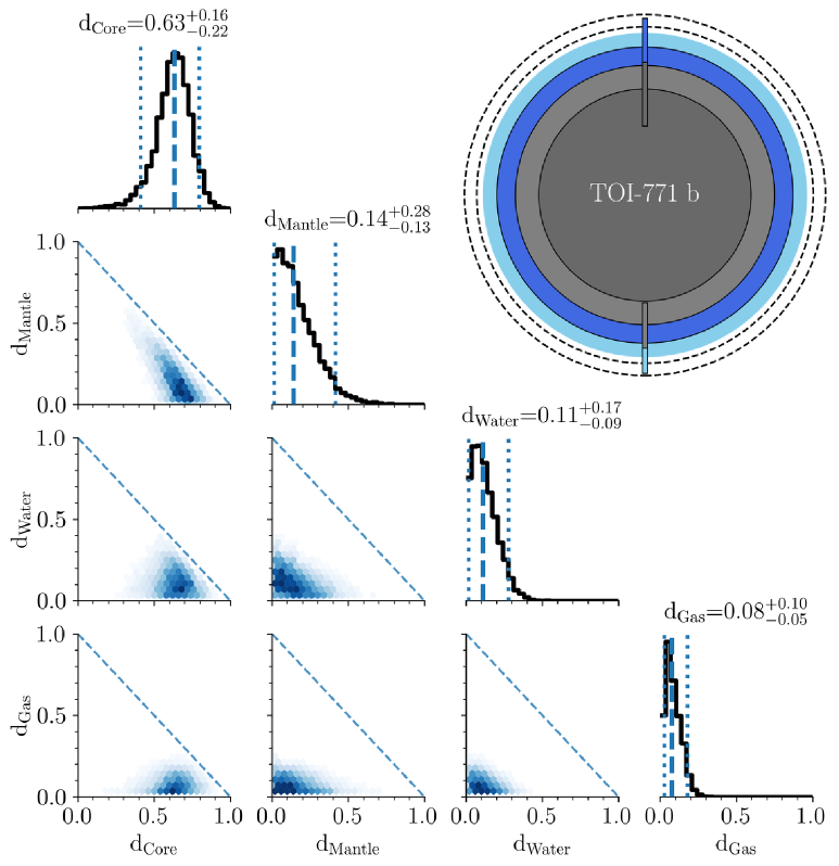
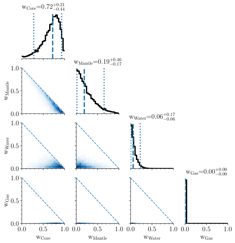
Figure 13: Left panel: predicted thickness (radius fraction, d) of the interior layers of TOI-771 b as computed with ExoMDN. The panel also features a sketch of the planet showing the radius fractions corresponding to the posterior distributions of the inner core, mantle, water layer, and gas envelope in dark grey, light grey, dark blue and light blue, respectively. The total uncertainty on the planetary radius is shown with the black dashed outer rings, while the uncertainties on each layers thickness are shown by coloured rectangles. Right panel: predicted mass fraction (w) of the interior layers of TOI-771 b as computed with ExoMDN.

When compared to the synthetic population models of (Venturini et al., 2024) for planets around M dwarfs, TOI-771 b’s position is consistent with the population of pure rocky cores. Hints of formation inside the water ice line arise from the small amount of volatiles suggested from the slightly lower planetary density with respect to a pure rocky core.

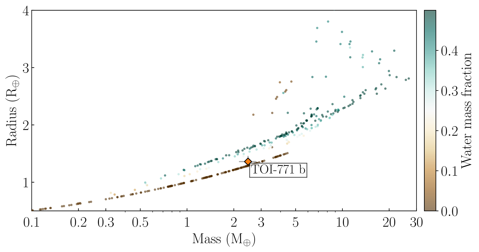
Figure 14: Theoretical mass-radius diagram for a synthetic population of planets at $2$ Gyr around an M dwarf with $M_{\star}$ $=0.4$ M_⊙, orbiting with periods $P<100$ d (Venturini et al., 2024). Each point represents a synthetic planet, and it is colour-coded according to its water mass fraction, with brown colours indicating purely rocky cores, and blue colours showing planets with a substantial amount of water (up to $50$%), as predicted from formation beyond the ice line (Alibert et al., 2013; Raymond et al., 2018; Bitsch et al., 2018; Brügger et al., 2020; Izidoro et al., 2021; Venturini et al., 2020). TOI-771 b is marked with an orange diamond, and it is consistent with the rocky population.

In line with the previous THIRSTEE results, TOI-771 b adds to the population of planets around M dwarfs with bulk density comparable to Earth’s identified in the $1.4-2$ R_⊕ regime by Luque & Pallé (2022). Such a population differs from a second, lower-density group of planets identified in the same radius range, which could be both enriched in volatiles (Luque & Pallé, 2022), or it might host a gaseous envelope (Rogers et al., 2023). This result further supports the hypothesis of the density gap in the observed small exoplanet population orbiting M dwarfs, initially proposed by Luque & Pallé (2022). The presence of such a density gap has been statistically confirmed by Schulze et al. (2024), and theoretically supported by formation and evolution models (Venturini et al., 2024), even though its significance and location is still debated, especially due to sample incompleteness in the low-mass regime (Parc et al., 2024). A larger, well-characterized sample will be crucial to assess the statistical significance of this density gap, as generally aimed by the THIRSTEE  project, and the characterisation of TOI-771 b significantly contributes to this goal.

6.2 The non-transiting candidate TOI-771 c

The retrieved semi-amplitude of TOI-771 c implies a minimum mass of $M_{\rm c}\sin{i}=2.87_{-0.38}^{+0.41}$ M_⊕ for the planet. We do not recover TOI-771 c with the current photometric dataset. Considering our injection-recovery tests, the planet is likely non-transiting, preventing the measure of the true planetary mass. For the TOI-771 system, even a small mutual inclination ($\Delta i\sim 1$ $\deg$) would allow planet c not to transit. In fact, considering the derived planetary and stellar parameters, the condition for showing a transit is $i_{\rm c}>88.64$ $\deg$, where the inclination of the inner planet is $i_{\rm b}=89.3\pm 0.5$ $\deg$.

Even though inclination cannot directly be constrained, according to Fischer et al. (2014) the planet has an 87% probability of having an inclination between 30 $\deg$ and 90 $\deg$ (Fischer et al., 2014), which implies a true mass lying within a factor two of the minimum mass, i.e. $M_{\rm p}$$\lesssim 5.82$ M_⊕. Assuming this mass value, the planet likely belongs to the sub-Neptune population (Parviainen et al., 2024). Additional constraint on the inclination can be derived considering the presence of the additional transiting companion TOI-771 b. In fact, based on population statistical studies, multi-planet systems with $a/$$R_{\star}$$>5$ tend to have mutual inclination $\Delta i\lesssim 5$ $\deg$ (Tremaine & Dong, 2012; Fang & Margot, 2012; Fabrycky et al., 2014; Dai et al., 2018). Assuming a mutual inclination of $\Delta i=5$ $\deg$ ($i_{\rm c}=84.3$ $\deg$), the planet would have a mass of $M_{\rm c}=2.92\pm 0.42$ M_⊕. A similarity between the masses of the two planets (with $M_{\rm b}=2.47_{-0.31}^{+0.32}$ M_⊕), is also expected from the so-called ‘peas in a pod’ pattern, according to which planets in the same system are likely to have similar masses (Millholland et al., 2017; Goyal & Wang, 2022), as well as orbital spacings and radii (Weiss et al., 2018). Finally, from our dynamical and stability analysis (Sect. 6.3), we derive a conservative mass upper limit of $11$ M_⊕, which confirms the sub-Neptune nature of the planet.

With an equilibrium temperature of $365_{-19}^{+22}$ K, TOI-771 c belongs to the warm temperature regime ($T_{{\rm eq}}$$<400$ K), however it is located outside the empirical habitable zone of its star, which embraces planets with periods $12$ d $<$ P $<73$ d (Kopparapu et al., 2013).

6.3 Dynamical analysis

To investigate the possible proximity of the TOI-771 system to mean motion resonances (MMRs) and the dynamical stability of our best-fit solution, we used direct $N$-body integrations and a CPU-efficient fast indicator called the Reversibility Error Method (REM; Panichi et al., 2017). REM is closely related to the Maximum Lyapunov Exponent (MLE). It is based on integrating the equations of motion with a time-reversible (symplectic) scheme back and forth for the same number of steps. Then the difference between the initial and final states of the system, normalised by the size of the phase-space trajectory, makes it possible to distinguish between regular and chaotic evolution. REM is scaled so that $\log\mathrm{\widehat{REM}}=0$ means that the difference between the initial and final states is of the order of the size of the orbit.

We integrated REM with the WHFAST integrator with the 17-th order corrector, with a fixed time step of $0.06$ d, as implemented in the REBOUND package (Rein & Liu, 2012; Rein & Tamayo, 2015) for $\simeq 2\times 10^{5}$ orbital periods of the outer planet. As shown in Fig. 15, our best-fit solution has $\log\mathrm{\widehat{REM}}$ $\leq$ -5, indicating a stable solution. Furthermore, the location of the best-fit model in phase space indicates its non-resonant character. The dynamical map shows the nominal system shifted by a few $\sigma$ from the 10:3 MMR in $(P_{\rm c},e_{\rm c})$ plane, and it shows a narrow limitation in the $3\sigma$ range due to the high-order resonance structure.

In the attempt to constrain the mutual inclination of the orbits using dynamics, we first computed the REM maps in the $(\Delta\Omega,i_{\rm c})$ plane, where $\Delta\Omega\in[0^{\circ},360^{\circ}]$ is the separation of the nodal lines of the orbits and $i_{\rm c}\in[1^{\circ},179^{\circ}]$ is the inclination of planet c. Then, the mutual inclination of the orbits is:

$$i_{\rm mut}=\cos i_{\rm b}\cos i_{\rm c}+\sin i_{\rm b}\cos i_{\rm c}\cos\Delta\Omega.$$ (1)

We show in Fig. 16 the results of the REM simulations, computed with an integration step of $0.02$ d. Perhaps non-intuitively, stable regions appear only in a portion of the parameter plane, outside mutual inclinations of approximately $i_{\rm mut}\in(75^{\circ},140^{\circ})$. This implies moderate mutual inclinations, in line with the discussion presented in Sect. 6.2. Considering that $i_{\rm b}=89.3^{\circ}\pm 0.5^{\circ}$, the inclination of TOI-771 c for a stable configuration is restricted to $i_{\rm c}\in(15^{\circ},165^{\circ})$, and therefore its mass must be at most $M_{\rm c}\simeq 11$ M_⊕.

The resulting scan of the $(\Delta\Omega,i_{\rm b})$ plane is reminiscent of the results for the Lidov-Kozai resonance (e.g., Shevchenko, 2017; Naoz et al., 2013). Due to the fact that the LK resonance can be suppressed by General Relativity (GR) perturbations (and star-planet tides) in the calculations we included the GR perturbations in the simplest, yet quantitatively correct and CPU-efficient form of the radial and conservative potential $\sim r^{-2}$ introduced by Nobili & Roxburgh (1986). The interactions considered make it possible to consciously reduce the range of external body masses.

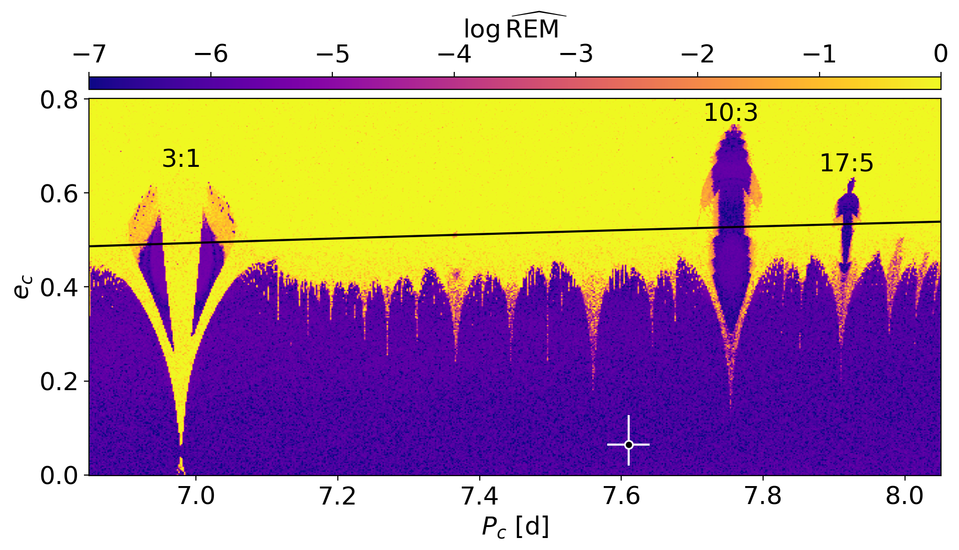
Figure 15: REM dynamical map for the solution presented in Table 4 in the $(P_{\rm c},e_{\rm c})$ plane of planet c. Small values of $\log\mathrm{\widehat{REM}}$ characterise regular (long-term stable) solutions, marked with a dark blue colour. Dynamically chaotic solutions are marked with lighter colours, up to yellow. Some of the MMRs producing dynamical features in the map are highlighted. The black curve represents the geometric collision of the orbits, defined by the condition: $a_{\rm b}(1+e_{\rm b})=a_{\rm c}(1-e_{\rm c})$. The white circle with crossed lines shows our best-fit solution with uncertainties. The resolution of the map is 601 $\times$ 301 points.

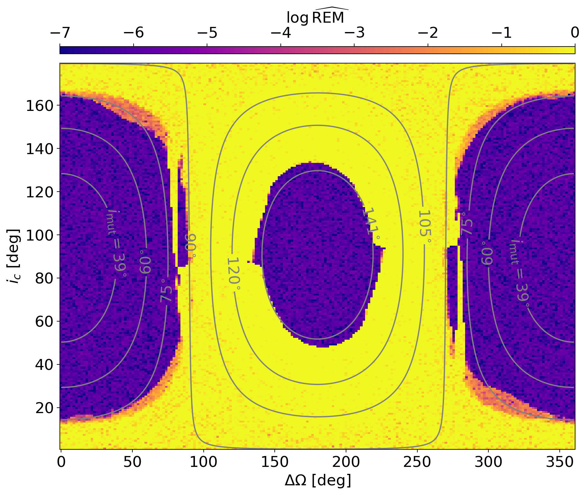
Figure 16: Dynamic REM map for several cycles of oscillation of the elements in the $(\Delta\Omega,i_{\rm c})$ plane. In addition to the gravitational interactions, GR perturbations are also included. The gray curves mark the levels of mutual inclination of the orbits.

6.4 Prospects for atmospheric characterisation

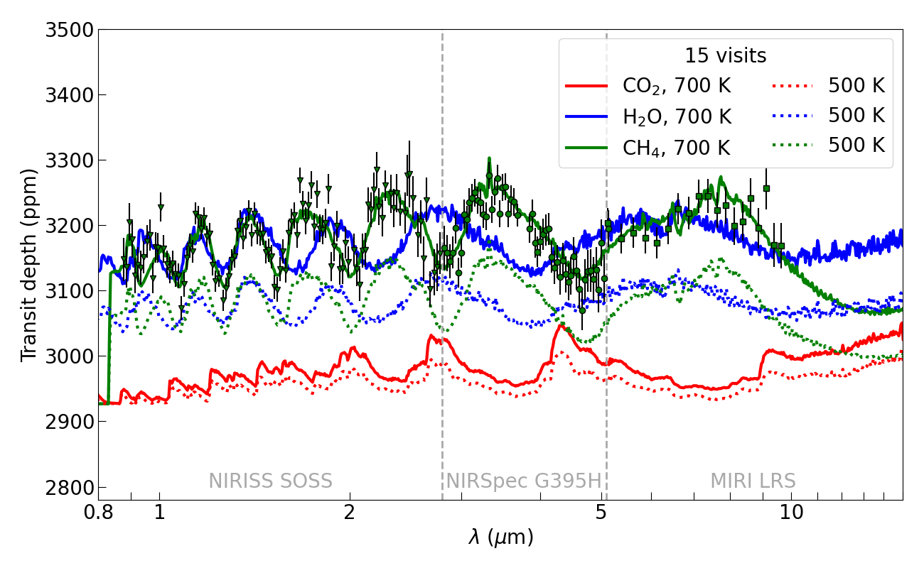
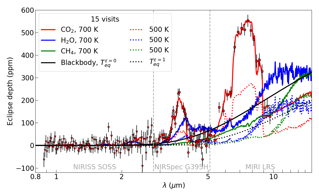
Figure 17: Modelled transmission (left) and emission (right) spectra of TOI-771 b, assuming an atmospheric composition of 100% CO₂ (red), 100% H₂O (blue), and 100% CH₄ (green) at different temperatures. For each composition we considered T-P profiles with equilibrium temperatures of 700 K (continuos) and 500 K (dashed line). Points with error-bars shows the simulated spectra for 15 transits/eclipses using the JWST NIRISS-SOSS, NIRSpec G395H, and MIRI LRS configurations.

To investigate the feasibility of TOI-771 b’s atmospheric characterisation, we calculated its transmission spectroscopy metric (TSM) and emission spectroscopy metric (ESM) following Kempton et al. (2018). With TSM $=15.5$ and ESM $=4.7$, TOI-771 b lies among the most favourable targets for both transmission and emission spectroscopy. In fact, the planet has a TSM higher than the threshold of $10$ proposed by Kempton et al. 2018 for $R_{\rm p}$ $<1.5$ R_⊕, and it is classified among the top five best-in-class targets for emission spectroscopy according to (Hord et al., 2024). The high precision on the planetary mass obtained from our analysis ($13$%) makes it an even more appealing target. In fact, a mass precision of at least $20$% is needed to break the degeneracy on compositional models and retrieve accurate atmospheric composition (Batalha et al., 2019).

We investigated the suitability of TOI-771 b for transmission and emission spectroscopy with the JWST by performing spectral simulations based on a tailored set of atmospheric models. We adopted TauREx 3 (Al-Refaie et al., 2021) to generate the synthetic spectra, using the stellar and planetary parameters from Tables 2 and 4. The atmospheric equilibrium temperature falls within the range of $\sim$500–700 K, depending on its Bond albedo and circulation efficiency, as derived in Section 5.3. We selected suitable temperature-pressure (T-P) profiles from the grid provided by Kempton et al. (2023). TOI-771 b has most likely lost its primordial H/He envelope, but it may possess a secondary atmosphere formed by mantle outgassing. We focused on three end-member compositions for the volatile-rich atmosphere: a water-world scenario with 100% H₂O, a Venus-like atmosphere with 100% CO₂, and an intriguing methane-world with 100% CH₄. Additionally, for completeness, we considered H/He atmospheres with 1$\times$ and 100$\times$ scaled solar abundances under chemical equilibrium, in both clear and hazy conditions, similar to those described in previous papers (e.g., Luque et al., 2022; Orell-Miquel et al., 2023; Goffo et al., 2024).

We used ExoTETHyS (Morello et al., 2021) to simulate the corresponding JWST spectra, as observed with the NIRISS-SOSS (0.6–2.8 $\mu$m), NIRSpec-G395H (2.88–5.20 $\mu$m), and MIRI-LRS (5–12 $\mu$m) instrumental modes. We adopted a spectral resolution of $R\sim$100 for NIRISS-SOSS and NIRSpec-G395H, and a constant bin size of 0.25 $\mu$m for MIRI-LRS, following the recommendations of the JWST Transiting Exoplanet Community Early Release Science team (Carter et al., 2024; Powell et al., 2024). The predicted error bars for a single transit observation are 49–197 ppm (mean error 88 ppm) for NIRISS-SOSS, 66–139 ppm (mean error 98 ppm) for NIRSpec-G395H, and 88–134 ppm (mean error 105 ppm) for MIRI-LRS.

Figure 17 shows the modelled transmission and emission spectra for the three steam atmosphere compositions, each paired with two distinct T-P profiles corresponding to equilibrium temperatures of 500 K and 700 K. The figure also overlays simulated spectra from 15 combined visits, for visualization purposes, for each instrumental mode. The transmission spectra exhibit small features of $\sim$100 parts per million (ppm) for the methane and water-world scenarios, with even smaller features for the Venus-like composition. This behaviour is unsurprising, as CO₂ has the largest molecular weight, corresponding to smaller atmospheric scale heights. The T-P profiles also affect the atmospheric scale heights, but the wavelength dependence is negligible, practically resulting in small offsets between models with the same chemistry. The emission spectra may display larger features at wavelengths $>$3 $\mu$m, reaching up to $\sim$600 ppm for the hotter CO₂ model and $\sim$300 ppm for the hotter H₂O model. The methane-world emission is the most similar to a blackbody spectrum. For all cases in emission, the spectral amplitudes are roughly halved when the cooler T-P profiles are assumed.

Observing multiple secondary eclipses of TOI-771 b with MIRI-LRS and/or NIRSpec-G395H would provide the best opportunity to determine its atmospheric composition. In the most favourable case of a Venus-like atmosphere with low circulation efficiency (dayside temperature $\sim$700 K), even one or two eclipses may suffice to detect strong CO₂ features. However, additional observations would be needed to distinguish a water-world from a methane-world or other configurations leading to blackbody-like spectra.

Observing multiple primary transits of TOI-771 b with NIRISS-SOSS and/or NIRSpec-G395H offers a viable alternative to detect an H₂O or CH₄-dominated atmosphere, but is less effective for heavier molecular weight compositions such as those of Venus and Earth. In the unlikely case of an H/He-dominated envelope with up to $\sim$100$\times$ solar metallicity, clear or hazy conditions, a single transit observation could easily reveal molecular absorption features (models not shown). However, clouds may attenuate absorption features in transmission, hindering their detection regardless of the atmospheric chemical composition. Another challenge for transit spectroscopy may arise from unocculted stellar spots on the M dwarf host, which can mimic water-world absorption features (e.g., Moran et al., 2023).

In summary, our simulations identify eclipse spectroscopy as the most promising technique to robustly detect and characterize the atmosphere of TOI-771 b (if present), owing to the possibility of larger spectral features in the mid-IR and a lower risk of contamination from stellar activity compared to transit spectroscopy. The success of this approach also depends on the atmospheric composition. For instance, a methane-world would emit less than 100 ppm at wavelengths below 10 $\mu$m, with a spectrum closely resembling that of an airless, reflective blackbody at the planetary equilibrium temperature. These scenarios could be distinguished by incorporating a precise measurement with the MIRI 15 $\mu$m photometer.

7 Conclusions

In this work, we used TESS and ground-based photometry, together with ultra-precise ESPRESSO RVs, to analyse one of the targets of the THIRSTEE project, the M-dwarf star TOI-771. We derived precise planetary parameters for TOI-771 b, a super Earth with an orbit of $2.32$ d and radius and mass of $R_{\rm b}=1.36\pm 0.10$ R_⊕, $M_{\rm b}=2.47_{-0.31}^{+0.32}$ M_⊕. Its bulk density ($\rho_{\rm b}=5.4\pm 1.4$ g cm^-3) makes it consistent with a rocky composition, even though a small amount of volatiles could be present. Additionally, we inferred from the RV dataset the presence of a second, non-transiting sub-Neptune in the system, TOI-771 c, with a minimum mass of $M_{\rm c}\sin{i}=2.87_{-0.38}^{+0.41}$ M_⊕  and a period of $7.61\pm 0.03$ d.

In line with previous THIRSTEE results, TOI-771 b supports the evidence of two populations with different composition around M dwarfs, separated by a density gap. With a high-precision mass ($13$%) and a warm effective temperature of $543_{-34}^{+28}$ K, the planet is a particularly interesting target for atmospheric characterisation, and it is included in the list of targets under consideration of the Rocky World Director’s Discretionary Time (DDT) program, a 500-hour JWST and HST program to investigate the atmosphere of terrestrial exoplanets orbiting M dwarfs (Redfield et al., 2024). Our simulations show that JWST eclipse spectroscopy is the most effective approach to detect and characterise the atmosphere of this planet (if present), and distinguish between a methane, CO₂, or water-dominated atmospheric composition.

The characterisation of the TOI-771 system provides a valuable addition to the sample of small, well-characterised planets around M dwarfs, pursuing one of the goals of the THIRSTEE project by enlarging the sample of well-characterised planets across spectral types, with the ultimate aim of understanding the sub-Neptune population under a global perspective.

Data availability

The ESPRESSO RVs and activity indicators (Table 5) are available in electronic form at the CDS via anonymous ftp to cdsarc.u-strasbg.fr (130.79.128.5) or via http://cdsweb.u-strasbg.fr/cgi-bin/qcat?J/A+A/.

Appendix A TESS target pixel files

We report in Fig. 18 the TPF images of TOI-771 for all TESS sectors except for sector 10, which is shown in Fig. 1.

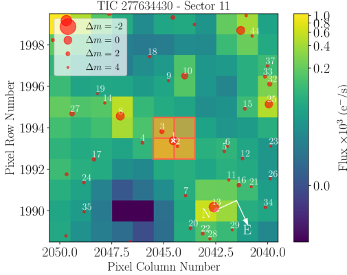
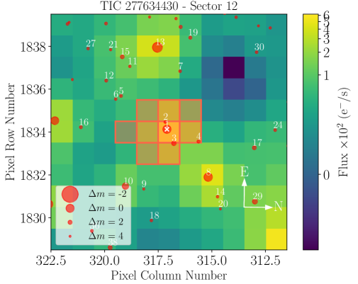
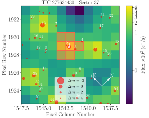
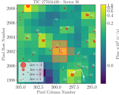
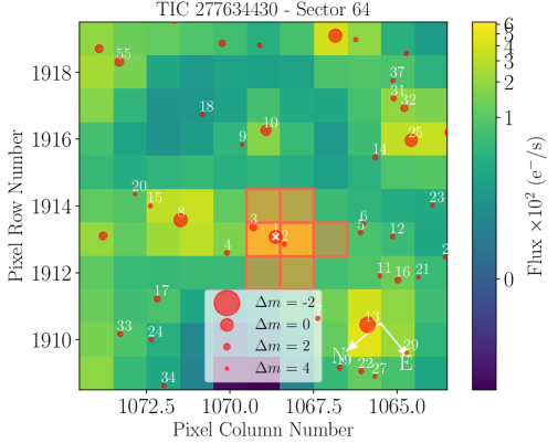
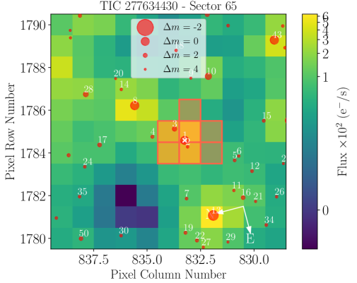
Figure 18: Same as Fig. 1, but for TESS sectors 11, 12, 37, 38, 64, 65.

Appendix B TESS light curves

We show in Fig. 19 the TESS SAP light curves of TOI-771 and the related GLS periodogram, searching for the rotational period of the star at $\sim 98$ d (Sect. 4.2). Such a long-period signal is difficult to identify in the current TESS photometry, as the clustering of the sectors in consecutive groups of two or three (S10, S11, S12; S37, S38; S64, S65), spread along the $\sim 4$ years of observations favour a shorter period of $\sim 37$ d, which is however not identified in any of the other activity indicators.

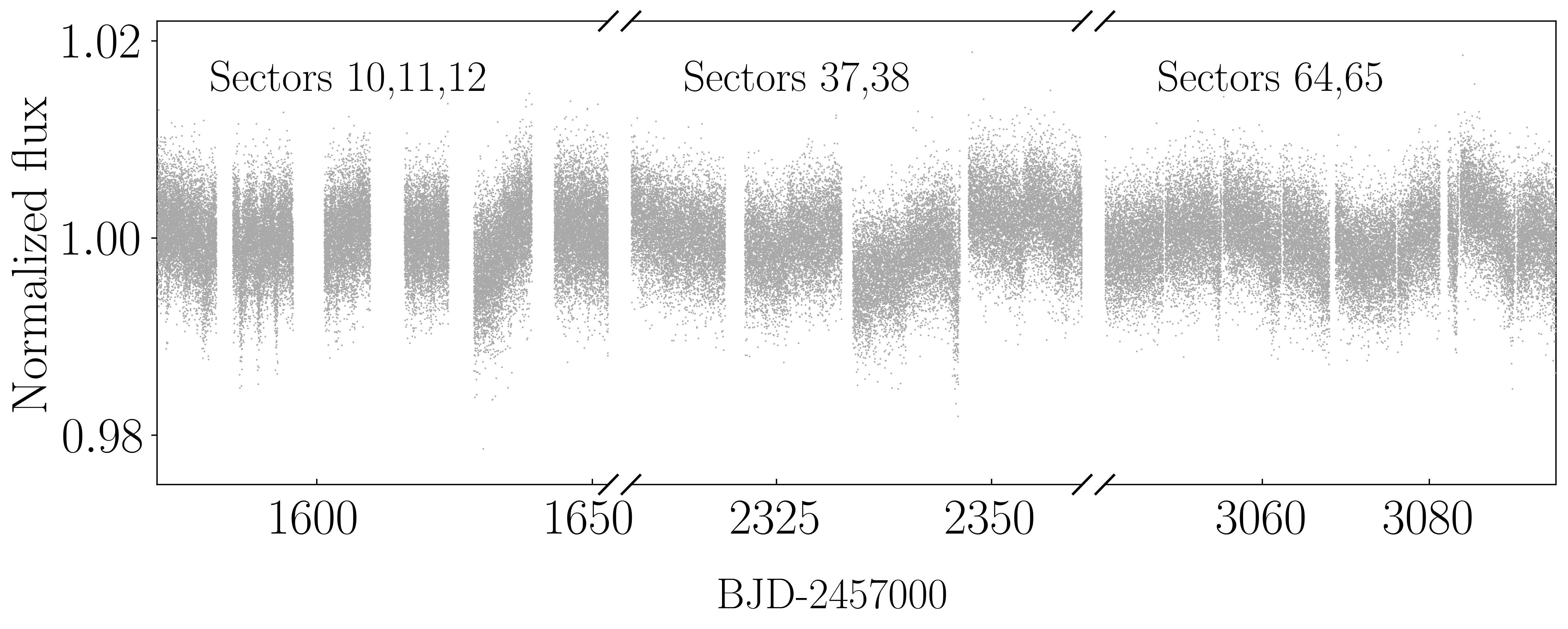
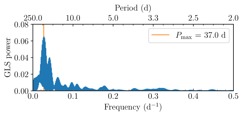
Figure 19: Top: TOI-771 TESS SAP light curves of TOI-771, grouped in consecutive sectors. Bottom: GLS periodogram of the whole TESS SAP light curve, with the most significant peak marked with a vertical orange line. The dashed line shows the 1% FAP probability.

We show in Figs. 20 the TESS light curves of TOI-771 modelled with the Matérn-3/2 kernel GP regression as described in Sect. 5.1). Figure  21 shows the pre-detrended TESS light curves with the best-fitting model as derived from the joint analysis described in Sect. 5.3.

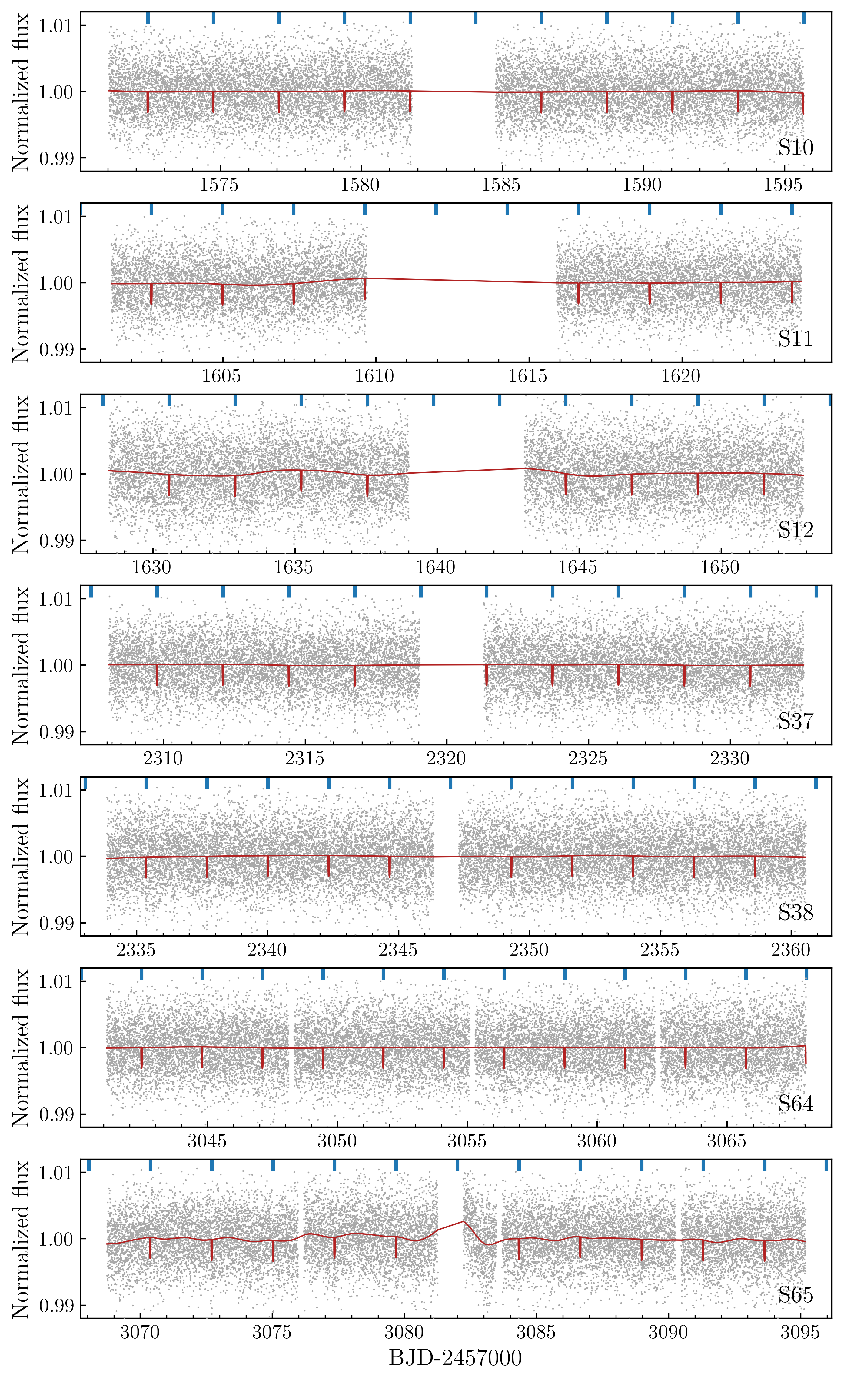
Figure 20: TOI-771 PDCSAP light curves of all available TESS sectors. The solid red line shows the photometric model including the Matérn-3/2 kernel GP regression (Sect. 5.1. The vertical blue lines highlight the transit ephemeris of TOI-771 b.

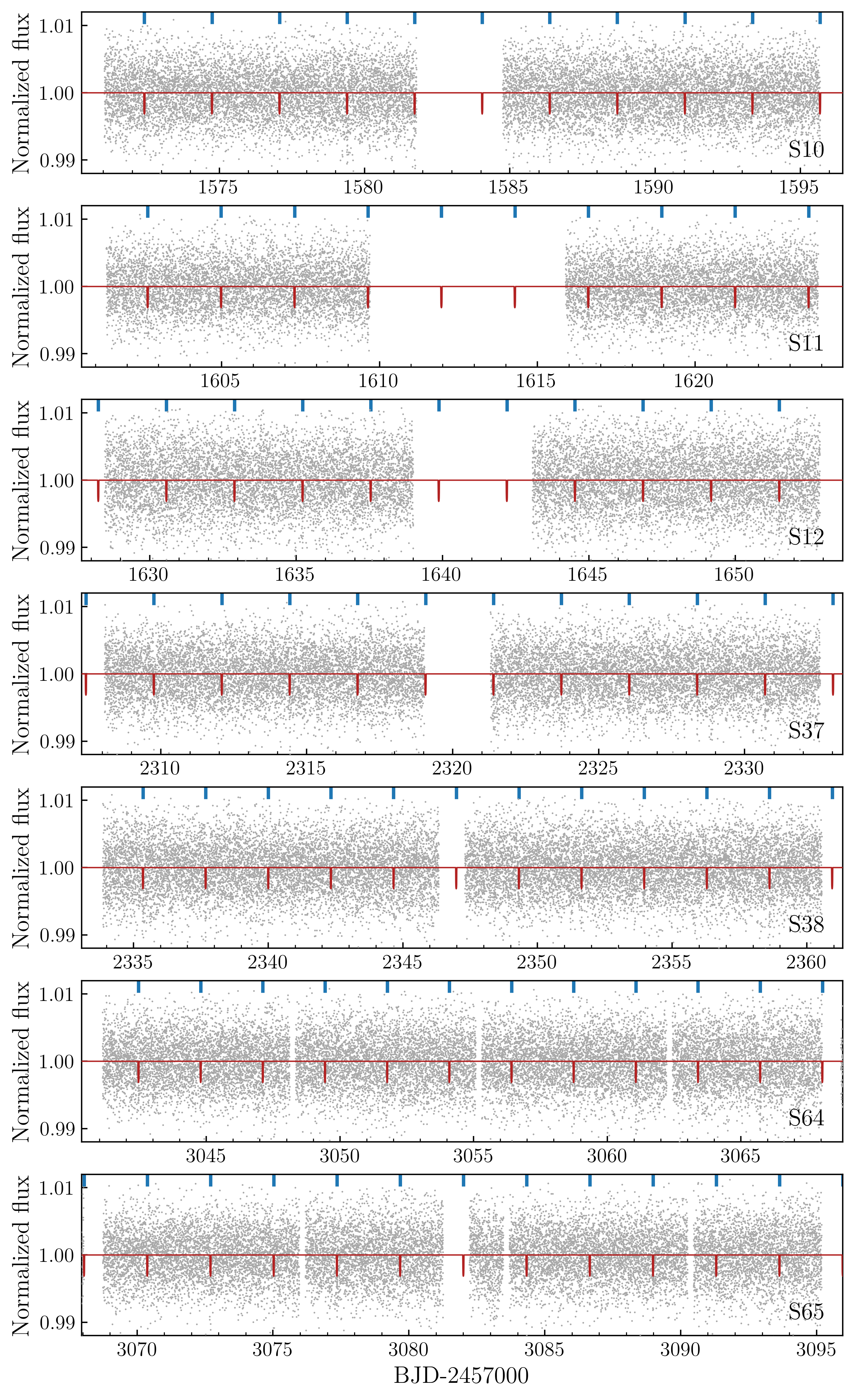
Figure 21: Same as Fig. 20, but using pre-detrended TESS light curves with no GP regression model. The solid red line shows the best-fitting model (Sect. 5.3).

Appendix C RV data

We list in Table 5 the ESPRESSO RVs and activity indicators collected for TOI-771.

Table 5: ESPRESSO RV measurements and activity indicators of TOI-771.

BJDTDB	RV	dLW	CRX	Na i D1	Na i D2	H$\alpha$	FWHM	BIS	$S$-index
$($d$)$	(m s-1)	(m2 s-2)	(m s-1)	(dex)	(dex)	(dex)	(m s-1)	(m s-1)
2460284.824724	$-4.39\pm 0.50$	$1.38\pm 0.21$	$6.0\pm 3.3$	$0.3312\pm 0.0059$	$0.2534\pm 0.0053$	$0.9510\pm 0.0028$	$2716.2\pm 2.6$	$-496.4\pm 2.5$	$0.946\pm 0.050$
2460289.774452	$-5.35\pm 0.58$	$1.10\pm 0.28$	$7.6\pm 3.9$	$0.3620\pm 0.0069$	$0.2665\pm 0.0061$	$0.9289\pm 0.0030$	$2718.7\pm 2.9$	$-562.0\pm 2.9$	$1.002\pm 0.070$
2460290.812825	$1.84\pm 0.59$	$1.21\pm 0.25$	$-3.0\pm 4.1$	$0.3408\pm 0.0067$	$0.2535\pm 0.0060$	$0.9657\pm 0.0031$	$22719.8\pm 2.9$	$-264.5\pm 2.9$	$1.172\pm 0.064$
…	…	…	…	…	…	…	…	…	…

Appendix D TTV search

We show in Figure 22 the TTVs of TOI-771 b computed as described in Section 5.3.

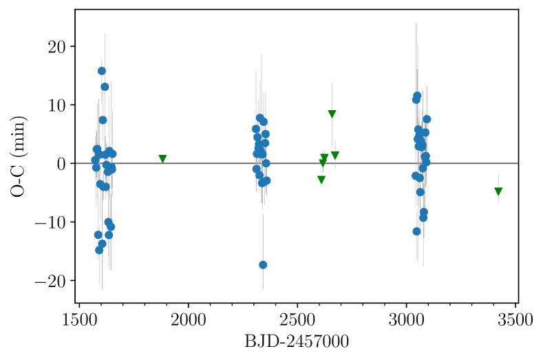
Figure 22: TTVs of TOI-771 b, measured computing the observed (O) minus calculated (C) transit times. Blue points show TESS transits, while green triangles refer to ground-based transit observations.