Quantum droplets in a beyond-mean-field density-dependent gauge theory
Abstract
The beyond-mean-field corrections appropriate to a bosonic many-body system experiencing a density-dependent gauge potential are derived, and from this the dimensional hierarchy of quantum droplet solutions are explored. Non-stationary quantum droplet solutions are supported by a single interaction parameter characterising the strength of the gauge potential, while in one dimension the beyond-mean-field theory can be solved exactly to yield chiral quantum droplets and dark soliton-like excitations. Numerical simulations of single and pairs of chiral droplets indicate a rich dynamics in the beyond-mean-field regime.
Introduction. Interactions underpin the emergence of a wide variety of quantum mechanical phenomena in condensed matter systems. Here, the particulars of the atoms statistics, dimensionality and potential environment contribute to the overall equilibrium description of the many-particle state. Prominent illustrations are given by superconductivity bruus_book and the family of quantum Hall effects klitzing_2020 in fermionic systems, while for bosonic systems the Lieb-Liniger franchini_book ; cazalilla_2011 and closely related Tonks-Girardeau models sowinski_2019 describe the many-body physics in this limit, possessing solutions which allow important insight into weakly and strongly coupled interacting many-body quantum gases mistakidis_2023 . Closely related to this, the BCS to BEC crossover remains an important concept for understanding the interplay of quantum statistics and many-body interactions ohashi_2020 ; strinati_2018 .
Over the last few years systems comprised from ensembles of bosonic particles possessing either magnetic dipole-dipole interactions kadau_2016 ; schmitt_2016 ; barbut_2016 or formed from binary mixtures cabrera_2018 ; semeghini_2018 ; cheiney_2018 ; ferioli_2019 ; derrico_2019 ; cavicchioli_2025 have received an intense amount of theoretical and experimental attention, due to the discovery and subsequent explanation of their ability to host droplet-like phases – where the weakly interacting system can exist in regimes where established theories predicted the collapse of the mean-field wave function. The stability of the liquid-like phase has been accounted for by beyond-mean-field corrections lima_2011 ; lima_2012 ; petrov_2015 to the ground state energy of the system in the form of the Lee-Huang-Yang (LHY) term lee_1957 .
Quantum droplet phases now represent an established paradigm within the quantum gas community. Studies have also focused on realizing pure LHY fluids jorgensen_2018 ; skov_2021 , extensions to coherently coupled systems chiquillo_2019 , spinor systems uchino_2010 ; yogurt_2023 , Bose-Fermi mixtures adhikari_2018 ; rakshit_2019 and understanding the fundamental physics of dipolar droplets in terms of the quantum fluctuations of the gas edler_2017 . Recently the enigmatic supersolid phase where off-diagonal and long-range order can paradoxically coexist was demonstrated in dipolar condensates tanzi_2019 ; bottcher_2019 ; chomaz_2019 . Parallel to investigations in quantum gas systems, droplet-like phases of matter have also been studied in the Helium fluids barranco_2006 , optomechanical walker_2022 , semiconductor hunter_2014 and optical systems realising photonic droplets wilson_2018 .
Ultracold quantum gases represent highly amenable platforms for simulating synthetic forms of matter, close to absolute zero where quantum mechanical effects can be clearly studied and accurately modelled schafer_2020 . Engineering synthetic degrees of freedom has allowed a series of state-of-the-art experiments to simulate orbital magnetism lin_2009 ; lin_2009b ; lin_2011 with quantum gases. While these accomplishments brought important effects from condensed matter into the cold atom realm such as spin-orbit coupling lin_2011b , spin-Hall phenomena beeler_2013 and synthetic dimensions celi_2014 ; a fundamental limitation existed in that these systems describe static gauge theories such that the gauge potential is not itself a dynamical object.
The last few years has seen the experimental demonstration of quasi-dynamical gauge theories where the synthetic gauge degree of freedom is coupled to the generally time-dependent quantum state of the system, thus providing a form of nonlinear feedback between the gauge and matter degrees of freedom. Pioneering experiments realised density-dependent gauge theories in optical lattice geometries for both bosons clark_2018 ; kwan_2024 and fermions gorg_2019 and also for an ensemble of Rydberg atoms lienhard_2020 . Following this two groups independently realised density-dependent gauge potentials in the continuum where a domain wall excitation was observed yao_2022 , and a type of topological gauge theory associated with the quantum Hall effect aglietti_1996 was realised frolian_2022 possessing an unusual type of edge mode in the form of a chiral soliton chisholm_2022 .
These synthetic forms of quasi-dynamical gauge theories have stimulated further questions regarding both the inherent phenomenology of these unusual systems; such as the nature of their nonlinear dingwall_2019 ; bhat_2021 ; jia_2022 ; chen_2022 ; zhang_2023 ; gao_2023 ; xu_2023 ; arazo_2023 ; faugno_2024 , spinor zezyulin_2018 ; xu_2021 ; abdullaev_2023 ; arazo_2024 and superfluid states bhat_2023 ; bhat_2024 ; gao_2024 as well as more fundamental goals concerning the route to simulating a truly dynamical gauge field with quantum gas systems rojas_2020 ; rojas_2023 . While existing theories account for density-dependent magnetism in the dilute weakly interacting limit, given the interest in beyond-mean-field phases, there is currently a gap in describing the phenomenology of this inherently many-body system in a regime where LHY physics comes into play. The purpose of this work is to derive such a theory appropriate to a system of many-body interacting bosons, and from this explore the allowed quantum droplet solutions across the parameter space of the model.
Beyond-mean-field model. We consider the following second-quantized Hamiltonian describing a system of interacting bosons
| (1) |
here defines the annihilation operator for a boson at position , while the gauge potential is defined as where a defines the vectorial strength of the density-dependent gauge potential while defines the dimensionally-dependent strength of the -wave interactions. Then the Heisenberg equation for is
| (2) |
where the second-quantized current operator is defined as
| (3) |
We transform Eq. (1) into momentum space which gives the total Hamiltonian where
| (4a) | ||||
| (4b) | ||||
| (4c) | ||||
Here defines the volume of the system and is the single-particle energy. The terms , , and contribute respectively the single, two and effective three-body interactions to the total Hamiltonian . Applying the Bogoliubov approximation pethick_book to the system (4) and diagonalizing the resulting quadratic Hamiltonian leads to the expression
| (5) |
where . Equation (5) introduces the canonical quasi-particle operator defined as satisfying , defines the homogeneous density, while the two amplitude functions are defined by and , where is the difference between the Hartree-Fock energy of a particle and the chemical potential . The diagonalized Hamiltonian’s eigenfunctions from Eq. (5) are given by Fock states where the momentum mode possesses Bogolon quasiparticles. The eigenvalue equation for the quasiparticle number operator is
| (6) |
and the Bogoliubov ground state associated with Eq. (6) is ueda_book . Corrections to the ground state energy can then be obtained from Eq. (5) from . The energy is divergent in , requiring regularization for both the two and three-dimensional cases. Defining , one obtains
| (7a) | ||||
| (7b) | ||||
| (7c) | ||||
Equations (7) introduce the three-dimensional scattering parameter and the energy cut-off arising from the infrared divergence of the momentum-space regularization of . In general the scattering parameters differ from the three-dimensional case due to the anisotropic geometry, resulting in a confinement induced resonance olshanii_1998 ; salasnich_2016 . Then, the total beyond-mean-field energy can be written in dimension using Eqs. (7) giving r_note
| (8) |
where , and Eq. (8) is obtained by transforming the classical field equation associated with Eq. (2) into the moving frame using the ansatz harikumar_1998 .
Quantum droplets. The purely mean-field model obtained from Eqs. (2) and (3) by taking the symmetry-breaking average already possesses an unusual nonlinear structure stemming from the nonlinear gauge potential . It is instructive to understand when this model manifests solutions in the parameter space. In what follows we work in the homogeneous limit which can be associated with a parameter regime where there are a large number of atoms constituting the quantum droplet. Without the LHY correction, Eq. (8) will in general admit solutions possessing a stable minima in the space if with a density obtained by minimizing the energy per particle petrov_2016 , giving . Then the mean-field chemical potential is found as
| (9) |
In the analysis that follows pertaining to the beyond-mean-field limit, we consider the purely gauge coupled system in the absence of the background scattering length gnote . Then at the mean-field level stable minima in with only exist when , a situation which changes when beyond-mean-field corrections are included. In what follows we take similar to the experimental works in the continuum yao_2022 ; frolian_2022 .
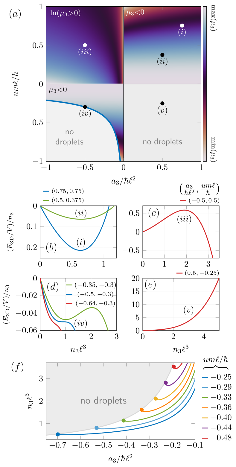
Figure 1 scrutinizes the allowed three-dimensional droplet solutions in the parameter space. Panel (a) shows heat maps of the beyond-mean-field chemical potential for all combinations of the signs of and . For the energy per particle possesses a single minima at finite positive ; examples of for this quadrant are shown in (b)(i) and (b)(ii). When the extrema of the energy per particle are given by unstable maxima with positive chemical potential , here (c)(iii) shows an example of this situation. If , quantum droplet states exist in a metastable regime where comprises a maxima and minima whose depth depends on the particular choice of and . This quadrant manifests points of inflection that comprise a border between the metastable droplets and a region where there are no droplets due to the energy per particle decreasing monotonically as shown in (d)(iv). The borderline between the stable and unstable region can be computed analytically as . This means that the effect of including beyond-mean-field corrections reduces the stable region of the parameter space in this quadrant compared to the pure mean-field model Eq. (9). Meanwhile the energy per particle for the final quadrant of (a) corresponding to does not possess any stable minima, instead monotonically increases as shown in (e)(v). The final panel of Fig. 1, (f) explores how the equilibrium density behaves as a function of the gauge potential strength in the quadrant. For a fixed value of , there exists a value of at which the solution terminates (see individual coloured data sets). The equilibrium density is found to increase for a given value of , with a sharp increase occurring as .
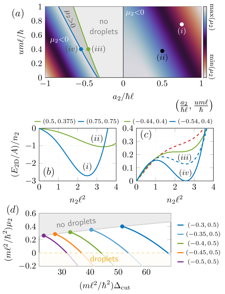
Next we examine the allowed droplet solutions in two-dimensions corresponding to Eqs. (7b) and (8), shown in Fig. 2. The two-dimensional regularization procedure is known to be infrared divergent, leading to the existence of a cut-off energy salasnich_2016 . Choices of the cut-off depend, in general on the low-energy scattering properties of the underlying model and are generally independent of the density of the gas. Here, we work with a fixed value of in Figs. 2(a)-(c). We have checked that altering the cut-off modifies our results only quantitatively, the specific choice here allowing a clear visual depiction of the key physical behaviours of the parameter space. Then, regions possessing droplet solutions are shown in panel (a) in the parameter space. Note that the two-dimensional energy per particle possesses the mirror symmetry hence only states with are depicted.
When or single minima are found with , see (b)(i) and (ii) for examples. The depth of the minima is found to increase when the strength of the gauge potential and velocity are simultaneously increased. Then for or the allowed solutions are separated into three regions. The energy per particle changes from being monotonically increasing (light grey region) to showing an inflection point (solid green line) to finally forming a metastable minima (solid blue line), each of which is depicted in (c). The dark grey region sandwiched between the inflection and metastable minima also possesses stable solutions – however the chemical potential here, which we do not associate with a bound droplet solution (dashed blue curve in (c)). The critical density at which the inflection point manifests can be shown to be
| (10) |
which is independent of the cut-off . In contrast to the two-dimensional mean-field result Eq. (9), the beyond-mean-field model can exhibit solutions in the attractive regime when . Finally panel (d) shows how the chemical potential depends on . The light grey shaded region corresponds to the red dashed curve in (c), while the border to the inflection region corresponds to the solid green in (a) and (c). The effect of changing is explored in (d). Here each of the coloured curves shows how varies for fixed as the strength of the two-dimensional gauge potential is changed. Each curve starting at an inflection point (coloured circles) decreases towards (dashed gold line) where bound two-dimensional droplets are predicted.
Low dimensional systems have provided ample opportunity for the exploration of quantum droplet phases, in particular one-dimensional models are often solvable, allowing deeper theoretical insight into the liquid-like state bottcher_2020 ; luo_2021 ; khan_2022 . Using Eqs. (2) and (7c) along with the local density approximation, an extended Gross-Pitaevskii equation can be obtained as
| (11) |
where the current operator is given by and . The gauge potential appearing in Eq. (11) can be decoupled using the Jordan-Wigner-like transformation aglietti_1996
| (12) |
which gives a current-coupled derivative cubic-quintic Schrödinger equation
| (13) |
along with the transformed current nonlinearity . Applying the transformation to Eq. (13) leads to the cubic quintic Schrödinger model . In writing Eq. (13) we have chosen the gauge potential strength such that motivated by the known solutions studied in nonlinear optics and strongly-interacting Bose gases birnbaum_2008 ; kolomeisky_2000 . Two classes of stable solutions exist, the first with vanishing boundary conditions gives rise to the quantum droplet solution
| (14) |
Analogous to the situation in higher dimensions the droplet solution in Eq. (14) possess an equilibrium density with associated chemical potential , while the total atom number can be found using as
| (15) |
with the length scale . We note that the atom number in Eq. (15) diverges as . Next we compute the surface tension of the quantum droplet in Eq. (14) defined as bulgac_2002 , where , which results in
| (16) |
Through the equilibrium chemical potential the surface tension depends in general on both the strength of the gauge potential and unusually the velocity of the quantum droplet. The surface tension will for fixed increase monotonically with , while for fixed will instead decrease with increasing .
The corresponding dark soliton-like solution is instead given by
| (17) |
with the asymptotic (vacua) appearing in Eq. (17) defined as . Then the function is given by
| (18) |
while the dimensionless function appearing in the definition of in Eq. (17) is given by . Equation (17) describes a propagating solitary wave whose amplitude develops a low-density region centred around the spatial origin that increases in size as . A regularized atom number kivshar_1998 can be associated with Eq. (17) defined as , given by
| (19) |
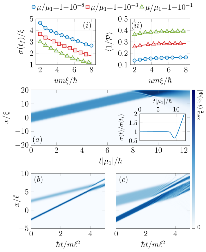
The dynamics of single and pairs of chiral droplets are explored in Fig. 3. The dynamics of a single quantum droplet solution to Eq. (13) with and is shown in (a). Here the droplet propagates before expanding due to collision with the edge of the numerical box. The inset computes the width as a function of time. To further quantify the dynamics, the droplet’s width as a function of velocity and time-averaged inverse participation ratio (IPR) with
| (20) |
are shown in panels (i) and (ii) respectively for three fixed values of . Smaller droplets (green triangles) correspond to the smallest values of and the largest values of . The IPR quantifies how localized a solution is. The larger droplets possess smaller values of due to the increased dominance of the beyond-mean-field term in Eq. (13). Panels (b) and (c) show the dynamics of a pair of droplets with and , with droplet normalizations (a) and (b). Increasing the atom number has the effect of changing the dynamics from particle-like (b) to showing non-integrable effects, where indeed the collision in (c) shows chiral droplet fusion. The initial phase difference between the droplets is in both cases.
Finally we can assess the viability of the theoretical predictions obtained in this work with experimental values. In the work of Frölian et al.,frolian_2022 , the current strength was given by
| (21) |
where defines the effective mass of the atoms, is the recoil momentum, is the radial length scale, encapsulates the -wave scattering lengths with , , and is the two-photon Rabi coupling strength. Using values appropriate for 39K and a radial trap strength haller_2009 , we obtain Js which along with a typical velocity gives a feasible one-dimensional equilibrium density of .
Outlook. We derived the beyond-mean-field (LHY) corrections appropriate to a density-dependent gauge theory which are free from the issues associated with the complex-valued beyond-mean-field ground state energy inherent to theoretical treatments of Bose-Bose and dipolar condensates cikojevi_2020 ; hu_2025 . We explored the dimensional-dependence of the droplet solutions, scrutinising the allowed stable equilibrium phases in the full two- and three-dimensional parameter space. Moving quantum droplet solutions in this model are supported by a single interaction parameter, and exist in regimes where the mean-field model is unstable in the two-dimensional case. In one dimension exact analytical solutions were obtained, along with an expression for the surface tension of the droplet. Numerical simulations explored the nonlinear dynamics of the beyond-mean-field model, revealing the fundamental phenomenology of the chiral droplet states.
The beyond-mean-field system explored in this work offers several opportunities for future work. Lower dimensional systems provide a wealth of phenomena with potential applications to quantum technologies like atomtronics amico_2021 . The allowed superfluid behaviour would also constitute an interesting avenue to explore, particularly the case for vortex states in two dimensions tengstrand_2019 where an additional rigid-body rotation would give insight into the topological physics of the model.
Acknowledgments. We thank Antonino Flachi, Stewart Lang, Antonio Muñoz Mateo, Joel Priestley, Gerard Valentí-Rojas and Ewan Wright for helpful discussions. This research was supported by the Australian Research Council Centre of Excellence in Future Low-Energy Electronics Technologies (Project No. CE170100039) and funded by the Australian government, and by the Japan Society of Promotion of Science Grant-in-Aid for Scientific Research (KAKENHI Grant No. JP20K14376).
References
- (1) H. Bruus and K. Flensberg, Quantum Theory in Condensed Matter Physics (Oxford University Press, 2006).
- (2) K. von Klitzing, T. Chackraborty, P. Kim, V. Madhaven, X. Dai, J. McIver, Y. Tokura, L. Savary, D. Smirnova, A. Maria Rey, C. Felser, J. Gooth, and X. Qi, Nat. Rev. Phys. 2, 397 (2020).
- (3) F. Franchini, An Introduction to Integrable Techniques for One-Dimensional Quantum Systems (Springer International Publishing, Cham, 2017).
- (4) M. A. Cazalilla, R. Citro, T. Giamarchi, E. Orignac, and M. Rigol, Rev. Mod. Phys. 83, 1405 (2011).
- (5) Tomasz Sowiński and Miguel Ángel García-March, Rep. Prog. Phys. 82, 104401 (2019).
- (6) S. I. Mistakidis, A. G. Volosniev, R. E. Barfknecht, T. Fogarty, Th. Busch, A. Foerster, P. Schmelcher, and N. T. Zinner, Phys. Rep. 1042, 1 (2023).
- (7) Y. Ohashi, H. Tajima, and P. van Wyk, Prog. Part. Nucl. Phys. 111, 103739 (2020).
- (8) G. C. Strinati, P. Pieri, G. Röpke, P. Schuck, and M. Urban, Phys. Rep. 738, 1 (2018).
- (9) H. Kadau, M. Schmitt, M. Wenzel, C. Wink, T. Maier, I. F.-Barbut, and T. Pfau, Nature 530, 194 (2016).
- (10) M. Schmitt, M. Wenzel, F. Böttcher, I. F.-Barbut, and T. Pfau, Nature 539, 259 (2016).
- (11) I. F.-Barbut, H. Kadau, M. Schmitt, M. Wenzel, and T. Pfau, Phys. Rev. Lett. 116, 215301 (2016).
- (12) C. R. Cabrera, L. Tanzi, J. Sanz, B. Naylor, P. Thomas, P. Cheiney, and L. Tarruell, Science 359, 301 (2018).
- (13) G. Semeghini, G. Ferioli, L. Masi, C. Mazzinghi, L. Wolswijk, F. Minardi, M. Modugno, G. Modugno, M. Inguscio, and M. Fattori, Phys. Rev. Lett. 120, 235301 (2018).
- (14) P. Cheiney, C. R. Cabrera, J. Sanz, B. Naylor, L. Tanzi, and L. Tarruell, Phys. Rev. Lett. 120, 135301 (2018).
- (15) G. Ferioli, G. Semeghini, L. Masi, G. Giusti, G. Modugno, M. Inguscio, A. Gallemí, A. Recati, and M. Fattori, Phys. Rev. Lett. 122, 090401 (2019).
- (16) C. D’Errico, A. Burchianti, M. Prevedelli, L. Salasnich, F. Ancilotto, M. Modugno, F. Minardi, and C. Fort, Phys. Rev. Research 1, 033155 (2019).
- (17) L. Cavicchioli, C. Fort, F. Ancilotto, M. Modugno, F. Minardi, A. Burchianti, Phys. Rev. Lett. 134, 093401 (2025).
- (18) A. R. P. Lima and A. Pelster, Phys. Rev. A 84, 041604(R) (2011).
- (19) A. R. P. Lima and A. Pelster, Phys. Rev. A 86, 063609 (2012).
- (20) D. S. Petrov, Phys. Rev. Lett. 115, 155302 (2015).
- (21) T. D. Lee, K. Huang, and C. N. Yang, Phys. Rev. 106, 1135 (1957).
- (22) N. B. Jørgensen, G. M. Bruun, and J. J. Arlt, Phys. Rev. Lett. 121, 173403 (2018).
- (23) T. G. Skov, Magnus G. Skou, N. B. Jørgensen, and J. J. Arlt, Phys. Rev. Lett. 126, 230404 (2021).
- (24) E. Chiquillo, Phys. Rev. A 99, 051601(R) (2019).
- (25) S. Uchino, M. Kobayashi, and M. Ueda, Phys. Rev. A 81, 063632 (2010).
- (26) T. A. Yoğurt, A. Keleş, and M. Ö. Oktel, Phys. Rev. A 107, 023322 (2023).
- (27) S. Adhikari, Laser Phys. Lett. 15, 095501 (2018).
- (28) D. Rakshit, T. Karpiuk, M. Brewczyk, and M. Gajda, SciPost Phys. 6, 079 (2019).
- (29) D. Edler, C. Mishra, F. Wächtler, R. Nath, S. Sinha, and L. Santos, Phys. Rev. Lett. 119, 050403 (2017).
- (30) L. Tanzi, E. Lucioni, F. Famà, J. Catani, A. Fioretti, C. Gabbanini, R. N. Bisset, L. Santos, and G. Modugno, Phys. Rev. Lett. 122, 130405 (2019).
- (31) F. Böttcher, J.-N. Schmidt, M. Wenzel, J. Hertkorn, M. Guo, T. Langen, and T. Pfau, Phys. Rev. X 9, 011051 (2019).
- (32) L. Chomaz, D. Petter, P. Ilzhöfer, G. Natale, A. Trautmann, C. Politi, G. Durastante, R. M. W. van Bijnen, A. Patscheider, M. Sohmen, M. J. Mark, and F. Ferlaino, Phys. Rev. X 9, 021012 (2019).
- (33) M. Barranco, R. Guardiola, S. Hernández, R. Mayol, J. Navarro, and M. Pi, J. Low Temp. Phys. 142, 1 (2006).
- (34) J. G. M. Walker, G. R. M. Robb, G.-L. Oppo, and T. Ackemann, Phys. Rev. A 105, 063305 (2022).
- (35) A. E. Almand-Hunter, H. Li, S. T. Cundiff, M. Mootz, M. Kira and S. W. Koch, Nature 506, 471 (2014).
- (36) K. E. Wilson, N. Westerberg, M. Valiente, C. W. Duncan, E. M. Wright, P. Öhberg, and D. Faccio, Phys. Rev. Lett. 121, 133903 (2018).
- (37) F. Schäfer, T. Fukuhara, S. Sugawa, Y. Takasu, and Y. Takahashi, Nat. Rev. Phys. 2, 411 (2020).
- (38) Y.-J. Lin, R. L. Compton, K. Jiménez-García, J. V. Porto, and I. B. Spielman, Nature 462, 628 (2009).
- (39) Y.-J. Lin, R. L. Compton, A. R. Perry, W. D. Phillips, J. V. Porto, and I. B. Spielman, Phys. Rev. Lett. 102, 130401 (2009).
- (40) Y.-Ju Lin, R. L. Compton, K. Jiménez-García, W. D. Phillips, J. V. Porto, and I. B. Spielman, Nat. Phys. 7, 531 (2011).
- (41) Y.-J. Lin, K. Jiménez-García, and I. B Spielman, Nature 471, 83 (2011).
- (42) M. C. Beeler, R. A. Williams, K. Jiménez-García, L. J. LeBlanc, A. R. Perry, I. B. Spielman, Nature 498, 201 (2013).
- (43) A. Celi, P. Massignan, J. Ruseckas, N. Goldman, I. B. Spielman, G. Juzeliūnas, and M. Lewenstein, Phys. Rev. Lett. 112, 043001 (2014).
- (44) L. W. Clark, B. M. Anderson, L. Feng, A. Gaj, K. Levin, and C. Chin, Phys. Rev. Lett. 121, 030402 (2018).
- (45) J. Kwan, P. Segura, Y. Li, S. Kim, A. V. Gorshkov, A. Eckardt, B. Bakkali-Hassani, and M. Greiner, Science 386, 1055 (2024).
- (46) F. Görg, K. Sandholzer, J. Minguzzi, R. Desbuquois, M. Messer, and T. Esslinger, Nat. Phys. 15, 1161 (2019).
- (47) V. Lienhard, P. Scholl, S. Weber, D. Barredo, S. de Léséleuc, R. Bai, N. Lang, M. Fleischhauer, H. P. Büchler, T. Lahaye, and A. Browaeys, Phys. Rev. X 10, 021031 (2020).
- (48) K.-X. Yao, Z. Zhang, and C. Chin, Nature 602, 68 (2022).
- (49) U. Aglietti, L. Griguolo, R. Jackiw, S.-Y. Pi, and D. Seminara, Phys. Rev. Lett. 77, 4406 (1996).
- (50) A. Frölian, C. S. Chisholm, E. Neri, C. R. Cabrera, R. Ramos, A. Celi, and L. Tarruell, Nature 602, 68 (2022).
- (51) C. S. Chisholm, A. Frölian, E. Neri, R. Ramos, L. Tarruell, and A. Celi, Phys. Rev. Research 4, 043088 (2022).
- (52) R. J. Dingwall and P. Öhberg, Phys. Rev. A 99, 023609 (2019).
- (53) I. A. Bhat, S. Sivaprakasam, and B. A. Malomed, Phys. Rev. E 103, 032206 (2021).
- (54) Q. Jia, H. Qiu, and A. M. Mateo, Phys. Rev. A 106, 063314 (2022).
- (55) L. Chen and Q. Zhu, New J. Phys. 24 053044, (2022).
- (56) A.-Q. Zhang, C. Jiao, Z.-F. Yu, J. Wang, A.-X. Zhang, and J.-K. Xue, Phys. Rev. E 107, 024218 (2023).
- (57) R. Gao, X. Qiao, Y.-E. Ma, Y. Jian, A.-X. Zhang and J.-K. Xue et al., Europhys. Lett. 141, 55003 (2023).
- (58) J. Xu, Q. Jia, H. Qiu, and A. M. Mateo, Phys. Rev. A 108, 053313 (2023).
- (59) M. Arazo, M. Guilleumas, R. Mayol, V. Delgado, and A. M. Mateo, Phys. Rev. A 108, 053302 (2023).
- (60) W. N. Faugno, Mario Salerno, and Tomoki Ozawa, Phys. Rev. Lett. 132, 023401 (2024).
- (61) D. A. Zezyulin, D. R. Gulevich, D. V. Skryabin, and I. A. Shelykh, Phys. Rev. B 97, 161302(R) (2018).
- (62) P. Xu, T.-Shu Deng, W. Zheng, and H. Zhai, Phys. Rev. A 103, L061302 (2021).
- (63) F. Kh. Abdullaev, M. S. A. Hadi, B. Umarov, L. A. Taib, and M. Salerno, Phys. Rev. E 107, 044218 (2023).
- (64) M. Arazo, M. Guilleumas, R. Mayol, V. Delgado, and A. M. Mateo, Phys. Rev. A 110, 023316 (2024).
- (65) I. A. Bhat, T. Mithun, and B. Dey, Phys. Rev. E 107, 044210 (2023).
- (66) I. A. Bhat and B. Dey, Phys. Rev. E 110, 024208 (2024).
- (67) M.-Z. Zhou, Y.-E. Ma, S.-D. Xu, L.-L. Mi, A.-X. Zhang, and J.-K. Xue, J. Phys. B: At. Mol. Opt. Phys. 57 125301 (2024).
- (68) G. Valentí-Rojas, N. Westerberg, and P. Öhberg, Phys. Rev. Research 2, 033453 (2020).
- (69) G. Valentí-Rojas, A. J. Baker, A. Celi, and P. Öhberg, Phys. Rev. Research 5, 023128 (2023).
- (70) C. J. Pethick and H. Smith, Bose-Einstein Condensation in Dilute Gases, (Cambridge University Press, Cambridge, 2002).
- (71) M. Ueda, Fundamentals and New Frontiers of Bose-Einstein Condensation, (World Scientific, Singapore, 2010).
- (72) M. Olshanii, Phys. Rev. Lett. 81, 938 (1998).
- (73) L. Salasnich and F. Toigo, Phys. Rep. 640, 1 (2016).
- (74) The term appearing in is not included in Eq. (8) so that the underlying mean-field theory agrees with existing works, Refs. aglietti_1996 ; chisholm_2022 . Including this term contributes only quantitatively to .
- (75) E. Harikumar, C. Nagaraja Kumar, and M. Sivakumar, Phys. Rev. D 58, 107703, (1998).
- (76) D. S. Petrov and G. E. Astrakharchik, Phys. Rev. Lett. 117, 100401 (2016).
- (77) One could also include the background -wave scattering term , but our goal here is to understand the interplay of the gauge and beyond-mean-field terms.
- (78) F. Böttcher, J.-N. Schmidt, J. Hertkorn, K. S. H. Ng, S. D. Graham, M. Guo, T. Langen, and T. Pfau, Rep. Prog. Phys. 84, 012403 (2020).
- (79) Z.-H. Luo, W. Pang, B. Liu, Y.-Y. Li, and B. A. Malomed, Font. Phys. 16, 32201 (2021).
- (80) A. Khan and A. Debnath, Front. Phys. 10, 887338 (2022).
- (81) Z. Birnbaum and B. A. Malomed, Physica D 237, 3252 (2008).
- (82) E. B. Kolomeisky, T. J. Newman, J. P. Straley, and X. Qi, Phys. Rev. Lett. 85, 1146 (2000).
- (83) A. Bulgac, Phys. Rev. Lett. 89, 050402 (2002).
- (84) Y. S. Kivshar and B. L.-Davies, Phys. Rep. 298, 81 (1998).
- (85) E. Haller, M. Gustavsson, M. J. Mark, J. G. Danzl, R. Hart, G. Pupillo, and H.-C. Nägerl, Science 325, 1224 (2009).
- (86) V. Cikojević, L. V. Markić, and J. Boronat, New J. Phys. 22 053045 (2020).
- (87) H. Hu, J. Wang, H. Pu, and X.-J. Liu, Phys. Rev. A 111, 023309 (2025).
- (88) L. Amico et al., AVS Quantum Sci. 3, 039201 (2021).
- (89) M. N. Tengstrand, P. Stürmer, E. Ö. Karabulut, and S. M. Reimann, Phys. Rev. Lett. 123, 160405 (2019).