Study of $K\pi$ final states from four-body deacy of $\bar{B}_{s}$ meason under perturbation QCD

Abstract

In the perturbative QCD framework, we use the quasi-two-body method to study the CP violations and branching ratios in the $\bar{B}_{s}\rightarrow[\phi(\rho^{0},\omega)\rightarrow K^{+}K^{-}][K^{*0}\rightarrow K^{+}\pi^{-}]$ and $\bar{B}_{s}\rightarrow[\rho^{0}(\omega,\phi)\rightarrow(\pi^{+}\pi^{-})][K^{*0}\rightarrow K^{+}\pi^{-}]$ decay processes. Owing to the interference effects of $\rho^{0}$, $\omega$, and $\phi$, new strong phases associated with vector mesons will be generated, resulting in relatively large CP violation within the interference region. Moreover, we provide numerical comparisons of CP violation from resonance effects and non-resonance contributions. In order to provide better theoretical predictions for future experiments, we integrate CP violation over invariant mass to obtain the regional CP violation value. Furthermore, we have calculated the polarization fractions and branching ratios for different intermediate states in the four-body decay process, which may be influenced by vector interference effects. Additionally, we discuss the possibility of observing the predicted CP violation at the LHC.

I Introduction

CP violation is a topic of great interest in the field of particle physics. Both theoretical and experimental efforts have been continuously exploring and searching for the origin of CP violation. In the Standard Model (SM), CP violation is mainly attributed to the Cabibbo-Kobayashi-Maskawa (CKM) matrix, which arises from the mixing and phase differences between quarks leading to CP violation in weak interaction Cabibbo:1963yz . At the same time, some resonance effects are related to complex strong phares, which may affect the CP violation in the decay process Zhang:2013oqa . The $\rho^{0}-\omega-\phi$ mixing mechanism can induce significant phase differences, leading to substantial CP violation within the interference range Li:2019xwh ; Shi:2022ggo ; Lu:2022rdi . Since the discovery of CP violation in the $K^{0}\bar{K}^{0}$ system in 1964 Christenson:1964fg , the study of CP violation has become increasingly profound and precise due to continuous advancements in experimental techniques and an increase in data KTeV:1999aiu ; Belle:2001zzw ; BaBar:2001oxa . In particular, the significant CP violation phenomenon observed during the multi-body decays of the B meson system provides a crucial experimental basis for in-depth research on the mechanism of CP violationLHCb:2012kja ; LHCb:2012uja ; Belle:2017cxf ; LHCb:2023exl . Therefore, multi-body decays have become a hot topic in recent years, providing clues for the revelation of new physics phenomena Bediaga:2013ela ; Cheng:2016shb ; Klein:2017xti ; Li:2018lbd ; Lu:2018fqe ; Ma:2019qlm ; LHCb:2019xmb ; LHCb:2019jta ; Yan:2022kck ; Liang:2022mrz .

B mesons contain heavy b quarks, making reliable calculation of perturbation effects for their decay processes. The large branching ratios of B meson also provide excellent plate for detecting CP violation Bander:1979px . The four-body decay of B mesons is more complex compared to two-body and three-body decays due to complex phase space. Specifically, four-body decay requires consideration of interactions and kinematics among more final-state particles, as well as more decay pathways. Due to the relatively limited research on B meson four-body decays, experimental and theoretical studies on this topic are of significant importance. Through in-depth investigation of the four-body decay process of B mesons, we can gain a more comprehensive understanding of the CP violation phenomena. Unexpectedly, we observe that the interference of vector mesons induces significant alterations in the polarization fractions and branching ratios within certain four-body decay processes. This finding also offers a valuable theoretical reference for experimental studies on the polarization fractions and branching ratios of four-body decays.

In this work, we used the perturbative QCD (PQCD) method to calculate the CP violation and branching ratio in the four-body decay process Lu:2000em ; Keum:2000ph ; Keum:2000wi . The PQCD method has been successfully applied to study the non-leptonic two-body decay processes of B mesons, achieving significant progress Xiao:2006mg . Typically, the multibody decay process involves sophisticated kinematics mechanisms, and the calculation of the corresponding hadronic matrix elements is not simple. However, in the quasi-two-body approach, the four-body decay process can be viewed as a quasi-two-body decay process with an intermediate resonance state Zhang:2025jlt ; Zou:2020fax ; Hua:2020usv . Therefore, the PQCD factorization formula for the studied four-body decay amplitude can be expressed as:

$$\begin{array}[]{ll}\mathcal{A}=A_{1}(\bar{B}_{s}\rightarrow V_{1}V_{2})A_{2}(V_{1}\rightarrow P_{1}P_{2})A_{3}(V_{2}\rightarrow P_{3}P_{4}),\\[7.0pt] \end{array}$$ (2)

for the decay process $\bar{B}_{s}\rightarrow V_{1}V_{2}$, its amplitude $A_{1}$ can be expressed as the convolution of the wave functions $\Phi_{B}$, $\Phi_{V_{1}}$, $\Phi_{V_{2}}$ and the hard kernel function ${\cal H}$, that is $\Phi_{B}\otimes{\cal H}\otimes\Phi_{V_{1}}\otimes\Phi_{V_{2}}$. Based on the formalism of Lepage, Brodsky, Botts, and Sterman, the PQCD factorization theorem has been developed for non-leptonic heavy meson decays Chang:1996dw ; Yeh:1997rq ; Lepage:1980fj ; Botts:1989kf . $A_{2}$ and $A_{3}$ represent the amplitudes of the $V_{1}\rightarrow P_{1}P_{2}$ and $V_{2}\rightarrow P_{3}P_{4}$ processes, respectively. Currently, extensive research has been carried out on the two-body decays of B mesons, and a large amount of data and research results related to B meson decays have been accumulated, including the CP violation phenomenon and the branching ratios Ali:2007ff . Therefore, under a mixing mechanism, we utilized the quasi-two-body method to calculate the CP violation and branching ratio in the $\bar{B}_{s}\rightarrow{(K^{+}K^{-})(K^{+}\pi^{-})}$ and $\bar{B}_{s}\rightarrow{(\pi^{+}\pi^{-})(K^{+}\pi^{-})}$ decay processes. By utilizing PQCD and quasi-two-body methods, we simplified the complex kinematics correlations, providing an effective computational framework for studying multi-body decays.

In the $\bar{B}_{s}\rightarrow V_{1}(V_{1}\rightarrow P_{1}P_{2})V_{2}(V_{2}\rightarrow P_{3}P_{4})$ decay process, $V_{1}$ and $V_{2}$ act as intermediate vector particles which subsequently decay into two hadrons. Specifically, $V_{1}$ decays into $P_{1}P_{2}$, while $V_{2}$ decays into $P_{3}P_{4}$. By using the factorization relation, also known as the narrow width approximation (NWA), we can effectively decompose this decay process into a continuous two-body decay:

$$\Gamma\left(\bar{B}_{s}\rightarrow V_{1}(V_{1}\rightarrow P_{1}P_{2})V_{2}(V_{2}\rightarrow P_{3}P_{4})\right)=\Gamma\left(B\rightarrow V_{1}V_{2}\right)\mathcal{B}\left(V_{1}\rightarrow P_{1}P_{2}\right)\mathcal{B}\left(V_{2}\rightarrow P_{3}P_{4}\right),$$ (3)

where $\Gamma$ represents the decay width and $\mathcal{B}$ represents the decay branching ratio. This method is only effective with narrow width limits, and it requires correction when the width becomes sufficiently large. Therefore, we introduce a correction factor:

$$\eta_{v_{12}}=\frac{\Gamma\left(B\rightarrow V_{1}V_{2}\right)\mathcal{B}\left(V_{1}\rightarrow P_{1}P_{2}\right)\mathcal{B}\left(V_{2}\rightarrow P_{3}P_{4}\right)}{\Gamma\left(\bar{B}_{s}\rightarrow V_{1}(V_{1}\rightarrow P_{1}P_{2})V_{2}(V_{2}\rightarrow P_{3}P_{4})\right)}.$$ (4)

The corrections to vector resonance typically fall below 10$\%$. When applying the QCD factorization method, the correction factor for decay processes is approximately around 7$\%$ Cheng:2020iwk ; Cheng:2020mna . When calculating CP violation, the constant $\eta_{v_{12}}$ can be eliminated without affecting the result, thereby disregarding the impact of the NWA on CP violation.

The article is structured as follows: In Sec. II, we provide a detailed explanation of the physical mechanism and calculation of mixing parameters based on the vector meson dominance (VMD) model, specifically focusing on the $\rho^{0}-\omega-\phi$ resonance effects. In Sec. III, we analyze the kinematics of the four-body decay process. In Sec. IV, we present typical Feynman diagrams and amplitude forms for first-order four-body decays within the framework of perturbative QCD (PQCD). In Sec. V, we conduct a comprehensive analysis of CP violation in the $\bar{B}_{s}\rightarrow{(K^{+}K^{-})(K^{+}\pi^{-})}$ and $\bar{B}_{s}\rightarrow{(\pi^{+}\pi^{-})(K^{+}\pi^{-})}$ decay processes under the $\rho^{0}-\omega-\phi$ vector meson resonance mechanism. Relevant parameters are provided in Sec. VI. The numerical results for CP violation, regional CP violation, polarization fractions, and branching ratios are presented in Sec. VII. Finally, in Sec. VIII, we summarize our findings and discuss the feasibility of observing the predicted CP violation at the LHC.

II VECTOR MESON MIXING MECHANISM

The vector meson dominance model (VMD) treats vector mesons as propagators interacting with photons Nambu:1957wzj ; Kroll:1967it . This model effectively elucidates the interaction between photons and hadrons. It plays a crucial role in our understanding of resonant states. Based on the VMD model, positron pairs annihilate to form photons. Subsequently, the resulting photons polarize in vacuum and generate vector particles such as $\rho^{0}(770)$, $\omega(782)$, and $\phi(1020)$. These vector particles then decay into $\pi^{+}\pi^{-}$ meson pair Ivanov:1981wf ; Achasov:2016lbc . In VMD model, the electromagnetic form factor of the $\pi$ meson is needed to obtain the mixing parameters corresponding to the two vector particles OConnell:1995nse . The contribution of the vector meson dominance model to the $e^{+}e^{-}\rightarrow\pi^{+}\pi^{-}$ process is illustrated in Fig. 1 and Fig. 2.

Figure 1: In the S-channel, electron-positron pairs annihilate into a photon, which subsequently decays into a $\pi^{+}\pi^{-}$ pair.

Figure 2: In the S-channel, the Vector Meson Dominance (VMD) model is employed to describe the process of $e^{+}e^{-}\rightarrow\pi^{+}\pi^{-}$.

The circle in Fig. 1 represents the form factor and represents all possible strong interactions that occur within the circle. We employ the VMD model to derive the description of the $e^{+}e^{-}\rightarrow\pi^{+}\pi^{-}$ process, as illustrated in Fig. 2. The mechanism of $\rho-\omega$ mixing arises from quark mass differences and electromagnetic interaction effects. In the QCD Lagrangian, quark mass differences lead to isospin symmetry breaking, causing hadrons such as $\rho$ and $\omega$ to interact with photons, thereby inducing mixing. A similar mechanism applies to $\rho-\phi$ mixing. Therefore, the contribution of isospin breaking to the process $e^{+}e^{-}\rightarrow\pi^{+}\pi^{-}$ from $\rho-\omega$ mixing and $\rho-\phi$ mixing at leading order is illustrated in Fig. 3.

Figure 3: The contributions of $\rho-\omega$ and $\rho-\phi$ mixing to the process $e^{+}e^{-}\rightarrow\pi^{+}\pi^{-}$.

Since the resonance state $\rho^{0}-\omega-\phi$ belongs to a non-physical state, in order to obtain its expression in the physical field, we need to transform the isospin field into the physical field through the unitary matrix R(s) Lu:2022rdi . There is a linear relationship between the physical state $\rho^{0}-\omega-\phi$ and the isospin state $\rho^{0}_{I}-\omega_{I}-\phi_{I}$, which is connected through the unitary matrix R(s): $A^{3\times 1}=R(s)A^{3\times 1}_{I}$. The matrix A comprises the elements $\rho^{0}$, $\omega$ and $\phi$, the matrix $A_{I}$ comprises the elements $\rho^{0}_{I}$, $\omega_{I}$ and $\phi_{I}$. And expression of R(s) is given as follows:

$$R(s)=\left(\begin{array}[]{lll}<\rho_{I}^{0}|\rho^{0}>&\hskip 8.5359pt<\omega_{I}|\rho^{0}>&\hskip 8.5359pt<\phi_{I}|\rho^{0}>\\[14.22636pt] <\rho_{I}^{0}|\omega>&\hskip 8.5359pt<\omega_{I}|\omega>&\hskip 8.5359pt<\phi_{I}|\omega>\\[14.22636pt] <\rho_{I}^{0}|\phi>&\hskip 8.5359pt<\omega_{I}|\phi>&\hskip 8.5359pt<\phi_{I}|\phi>\end{array}\right)=\left(\begin{array}[]{ccc}1&\hskip 8.5359pt-F_{\rho^{0}\omega}(s)&\hskip 8.5359pt-F_{\rho^{0}\phi}(s)\\ \\ F_{\rho^{0}\omega}(s)&\hskip 8.5359pt1&\hskip 8.5359pt-F_{\omega\phi}(s)\\ \\ F_{\rho^{0}\phi}(s)&\hskip 8.5359ptF_{\omega\phi}(s)&\hskip 8.5359pt1\end{array}\right),$$ (5)

where $<\rho_{I}^{0}|\omega>$, $<\rho_{I}^{0}|\phi>$, $<\omega_{I}|\phi>$ and $F_{\rho^{0}\omega}(s)$, $F_{\rho^{0}\phi}(s)$, $F_{\omega\phi}(s)$ are all first-order approximations terms. Based on the isospin representation, we construct the isospin base vector $|I,I_{3}>$, where $I$ and $I_{3}$ represent the isospin and its third component, respectively. Subsequently, we used an orthogonal normalization relation to establish the relationship between physical states and isospin states. Then we can obtain the expression of ${\rho^{0}}$, $\omega$ and $\phi$ in the physical field:

$$\begin{split}\rho^{0}=\rho_{I}^{0}-F_{\rho^{0}\omega}(s)\omega_{I}-F_{\rho^{0}\phi}(s)\phi_{I},\\ \\ \omega=F_{\rho^{0}\omega}(s)\rho_{I}^{0}+\omega_{I}-F_{\omega\phi}(s)\phi_{I},\\ \\ \phi=F_{\rho^{0}\phi}(s)\rho_{I}^{0}+F_{\omega\phi}(s)\omega_{I}+\phi_{I}.\end{split}$$ (6)

Furthermore, the mixed parameters $\Pi_{\rho^{0}\omega}$, $\Pi_{\rho^{0}\phi}$, $\Pi_{\omega\phi}$ and $F_{\rho^{0}\omega}$, $F_{\rho^{0}\phi}$, $F_{\omega\phi}$ are are order of $\mathcal{O}(\lambda)$ ($\lambda\ll 1$), while their multiplication yields higher order terms that can be disregarded in this processLu:2022rdi . Consequently, we obtain the expression of $F_{\rho^{0}\omega}$, $F_{\rho^{0}\phi}$, $F_{\omega\phi}$ as follows:

$$\begin{split}F_{\rho^{0}\omega}=\frac{\Pi_{\rho^{0}\omega}}{s_{\rho^{0}}-s_{\omega}},\hskip 8.5359pt\,F_{\rho^{0}\phi}=\frac{\Pi_{\rho^{0}\phi}}{s_{\rho^{0}}-s_{\phi}},\hskip 8.5359pt\,F_{\omega\phi}=\frac{\Pi_{\omega\phi}}{s_{\omega}-s_{\phi}}.\end{split}$$ (7)

The relationship between $F_{V_{1}V_{2}}$=$-F_{V_{2}V_{1}}$ can be observed. We define the propagator by combining the meson width dependent on energy with the meson mass and momentum. $s_{V}$ represents the inverse propagator of the vector meson $(V=\rho^{0}$, $\omega$ or $\phi)$, and we define $s_{V}=s-m_{V}^{2}+\mathrm{i}m_{V}\Gamma_{V}$. $m_{V}$ signifies the mass of the vector meson, $\Gamma_{V}$ is the decay width of a vector meson related to energy, and $\sqrt{s}$ corresponds to the invariant mass of a pair of $P_{1}P_{2}$ mesons.

In this paper, we introduce the momentum-related mixed parameter $\Pi_{V_{1}V_{2}}$ to achieve a noticeable s-dependence Lu:2023yxa . Wolfe and Maltnan accurately measured the mixed parameter $\Pi_{\rho^{0}\omega}=-4470\pm 250\pm 160-i(5800\pm 2000\pm 1100)\mathrm{MeV}^{2}$ near meson $\rho^{0}$ Wolfe:2009ts ; Wolfe:2010gf . The mixing parameter $\Pi_{\omega\phi}=19000+i(2500\pm 300)\mathrm{MeV}^{2}$ is determined near the $\phi$ meson. Moreover, the mixed parameter $\Pi_{\phi\rho^{0}}=720\pm 180-i(870\pm 320)\mathrm{MeV}^{2}$ is obtained near the $\phi$ meson Achasov:1999wr . Then we define :

$$\begin{split}\widetilde{\Pi}_{\rho^{0}\omega}=\frac{s_{\rho^{0}}\Pi_{\rho^{0}\omega}}{s_{\rho^{0}}-s_{\omega}},\hskip 8.5359pt\,~~\widetilde{\Pi}_{\rho^{0}\phi}=\frac{s_{\rho^{0}}\Pi_{\rho^{0}\phi}}{s_{\rho^{0}}-s_{\phi}},\hskip 8.5359pt\,~~\widetilde{\Pi}_{\phi\omega}=\frac{s_{\phi}\Pi_{\phi\omega}}{s_{\phi}-s_{\omega}}.\end{split}$$ (8)

III FOUR-BODY DECAY KINEMATICS

Compared to the kinematics of two-body decay, the kinematics of four-body decay is significantly more intricate. Currently, there is extensive research on the kinematics of four-body hadronic decay Pais:1968zza ; Kane:1978ie ; Lee:1992ih ; Kramer:1992ag . The process of four-body decay not only encompasses contributions from resonant and non-resonant components but also involves interactions among the final-state particles Grozin:1983tt ; Grozin:1986at ; Muller:1994ses ; Diehl:1998dk ; Diehl:2000uv ; Hagler:2002nf . The $\bar{B}_{s}\rightarrow V_{1}(V_{1}\rightarrow P_{1}P_{2})V_{2}(V_{2}\rightarrow P_{3}P_{4})$ process involves the decay of a $\bar{B}_{s}$ meson into two vector mesons, $V_{1}$ and $V_{2}$. Subsequently, $V_{1}$ decays into a pair of pseudoscalar mesons, $P_{1}$ and $P_{2}$, while $V_{2}$ decays into another pair of pseudoscalar mesons, $P_{3}$ and $P_{4}$.

Figure 4: The decay diagrams of $\bar{B}_{s}\rightarrow V_{1}(V_{1}\rightarrow P_{1}P_{2})V_{2}(V_{2}\rightarrow P_{3}P_{4})$ process.

As illustrated in Fig. 4, $P$, $p_{1}$, $p_{2}$, $q_{1}$ and $q_{2}$ denote the momenta of the $\bar{B}_{s}$ meson and the final-state four mesons respectively. For $\bar{B}_{s}$ meson with initial spin 0, the phase space integral in its four-body decay process depends on five variables: the three helicity angles and the square of the invariant masses of the two final meson pairs. These variables encompass:

(1). $s_{1}=(p_{1}+p_{2})^{2}$, the square of the invariant mass of the $P_{1}P_{2}$ meson pair.

(2). $s_{2}=(q_{1}+q_{2})^{2}$, the square of the invariant mass of the $P_{3}P_{4}$ meson pair.

(3). $\theta_{1}$, the angle between the direction of motion of $P_{1}$ in the rest frame of the $V_{1}$ meson and the direction of motion of the $V_{1}$ meson in the rest frame of the $\bar{B}_{s}$ meson.

(4). $\theta_{2}$, the angle between the direction of motion of $P_{3}$ in the rest frame of the $V_{2}$ meson and the direction of motion of the $V_{2}$ meson in the rest frame of the $\bar{B}_{s}$ meson.

(5). $\varphi$, the angle between the plane defined by the $P_{1}P_{2}$ meson pair and the plane defined by the $P_{3}P_{4}$ meson pair in the rest frame of the $\bar{B}_{s}$ meson.

$\Omega$ represents the phase space of four-body decay process, where $\mathrm{d}\Omega=X\alpha\beta ds_{1}ds_{2}d\cos\theta_{1}d\cos\theta_{2}d\varphi~$. The partial decay width is defined as follows:

$$d\Gamma=\frac{|{\cal M}|^{2}}{4(4\pi)^{6}m_{B}^{3}}X\alpha\beta ds_{1}ds_{2}d\cos\theta_{1}d\cos\theta_{2}d\varphi~,$$ (9)

where $|{\cal M}|^{2}$ represents the square of the amplitude Hsiao:2017nga . $X$, $\alpha$, and $\beta$ are represented respectively:

$$X=[(m_{B}^{2}-s_{1}-s_{2})^{2}/4-s_{1}s_{2}]^{1/2}\,,$$

$$\alpha=\lambda^{1/2}(s_{1},m_{p1}^{2},m^{2}_{p2})/s_{1}\,,$$

$$\beta=\lambda^{1/2}(s_{2},m_{q1}^{2},m^{2}_{q2})/s_{2}\,.$$ (10)

with $\lambda(a,b,c)=a^{2}+b^{2}+c^{2}-2ab-2bc-2ca$.

The permissible range of the five variables, on which the phase space integral depends, is defined as follows:

$$(m_{p1}+m_{p2})^{2}\leq \,s_{1}\, \leq(m_{\bar{B}_{s}}-\sqrt{s_{2}})^{2}\,,$$

$$(m_{q1}+m_{q2})^{2}\leq \,s_{2}\, \leq(m_{\bar{B}_{s}}-m_{p1}-m_{p2})^{2}\,,$$

$$0\leq\theta_{1,2}\leq\pi \,, 0\leq\varphi\leq 2\pi\,.$$ (11)

We can derive the branching ratio formula:

$$\mathcal{B}=\frac{\tau_{\bar{B}_{s}}}{4(4\pi)^{6}m_{\bar{B}_{s}}^{3}}\int{X\alpha\beta ds_{1}ds_{2}d\cos\theta_{1}d\cos\theta_{2}d\varphi|{\cal M}|^{2}}~,$$ (12)

where $\tau_{\bar{B}_{s}}$ refers to the lifetime of $\bar{B}_{s}$ meson.

IV THE AMPLITUDE OF THE QUASI-TWO-BODY DECAY PROCESS IN THE PERTURBATIVE QCD FRAME

In the PQCD factorization method, the non-leptonic decay of B mesons is dominated by the exchange of hard gluons. The hard part of the decay process is separated and treated using perturbation theory, while the non-perturbative part is absorbed into the universal hadron wave function. According to the “color transparency mechanism” in the initial state of the B-meson, the decay of the B meson causes the light quark to move at a high speed. For the spectator quark inside the B meson to gain large momentum and produce a fast-moving final meson with the light quark, a hard gluon is needed to provide energy. Thus the two “final state” vector mesons continue to decay, eventually producing four final state particles. The specific Feynman diagram is as follows:

Figure 5: The Feynman diagrams of $\bar{B}_{s}\rightarrow V_{1}(V_{1}\rightarrow P_{1}P_{2})V_{2}(V_{2}\rightarrow P_{3}P_{4})$ process.

Typical Fig.5 is leading-order Feynman diagram for the four-body decay, where the symbol •represents the weak interaction vertex. Diagrams (a)-(d) represents the emission contribution and diagrams (e)-(h) represents the annihilation contribution, with possible four-quark operator insertions. Using the quasi-two-body method, the total amplitude of $\bar{B}_{s}\rightarrow V_{1}(V_{1}\rightarrow P_{1}P_{2})V_{2}(V_{2}\rightarrow P_{3}P_{4})$ consists of two components: $\bar{B}_{s}\rightarrow V_{1}V_{2}$ and $V_{1}V_{2}\rightarrow{(P_{1}P_{2})(P_{3}P_{4})}$. When calculating the decay amplitude of $\bar{B}_{s}\rightarrow V_{1}V_{2}$, where the intermediate particles consist of two vector mesons, the vector mediators exhibit three polarizations: longitudinal (L), normal (N), and transverse (T). The amplitude is also characterized by the polarization states of these vector mediators.

In this paper, we define the momenta of $\bar{B}_{s}$ meson and two vector mesons using light-cone coordinates. By analyzing the Lorentz structure, its decay amplitude is decomposed into the following form Chen:2002pz ; Lu:2005be ; Li:2004ti ; Huang:2005if :

$$A^{(\sigma)}_{1} = \epsilon^{*}_{1\mu}\epsilon^{*}_{2\nu}(ag^{\mu\nu}+\frac{b}{M_{1}M_{2}}P^{\mu}P^{\nu}+\frac{ic}{M_{1}M_{2}}\epsilon^{\mu\nu\alpha\beta}P_{1\alpha}P_{2\beta})$$ (13)

$$= M^{2}_{\bar{B}_{s}}A_{L}+M^{2}_{\bar{B}_{s}}A_{N}\epsilon^{*}_{2}(\sigma=T)\cdot\epsilon^{*}_{3}(\sigma=T)+iA_{T}\epsilon^{\alpha\beta\gamma\rho}\epsilon^{*}_{2\alpha}(\sigma)\epsilon^{*}_{3\beta}(\sigma)P_{2\gamma}P_{3\rho}\;,$$

The superscript $\sigma$ indicates the helicity states of two vector mesons, where L (T) respectively represent the longitudinal (transverse) components. We can define the longitudinal $H_{0}$, transverse $H_{\pm}$ helicity amplitudes as :

$$H_{0}=M^{2}_{\bar{B}_{s}}{\cal A}_{L}\,,$$

$$H_{\pm}=M^{2}_{\bar{B}_{s}}{\cal A}_{N}\mp M_{1}M_{2}\sqrt{r^{{}^{\prime}2}-1}{\cal A}_{T}\,.$$ (14)

In the equation $r^{{}^{\prime}2}=\frac{P_{V_{1}}\cdot P_{V_{2}}}{M_{1}M_{2}}=\frac{M^{2}_{\bar{B}_{s}}}{2M_{1}M_{2}}$, $P_{V_{1}}$ and $P_{V_{2}}$ denote the momenta of the two vector particles, while $M_{1}$ and $M_{2}$ represent their respective masses. These quantities satisfy the following equation:

$$\sum_{\sigma}{A_{1}}^{(\sigma)\dagger}{A_{1}^{(\sigma)}}=|H_{0}|^{2}+|H_{+}|^{2}+|H_{-}|^{2}.$$ (15)

There exists another equivalent set of definitions for the helicity amplitudes:

$$A_{0} = -\xi M^{2}_{\bar{B}_{s}}{\cal A}_{L},$$

$$A_{\parallel} = \xi\sqrt{2}M^{2}_{\bar{B}_{s}}{\cal A}_{N},$$

$$A_{\perp} = \xi M_{1}M_{2}\sqrt{2(r^{{}^{\prime}2}-1)}{\cal A}_{T}\;,$$ (16)

with $\xi$ the normalization factor to satisfy $|A_{0}|^{2}+|A_{\parallel}|^{2}+|A_{\perp}|^{2}=1$, where the notations $A_{0}$, $A_{\parallel}$, $A_{\perp}$ denote the longitudinal, parallel, and perpendicular polarization amplitude.

In the process $V_{1}\rightarrow P_{1}P_{2}$, the amplitude is given by $A_{V_{1}\rightarrow P_{1}P_{2}}^{\lambda}=g_{V_{1}}\epsilon(\lambda)\cdot(p_{1}-p_{2})$, and for the process $V_{2}\rightarrow P_{3}P_{4}$, the amplitude is $A_{V_{2}\rightarrow P_{3}P_{4}}^{\gamma}=g_{V_{2}}\epsilon(\gamma)\cdot(q_{1}-q_{2})$. Here, $g_{V}$ represents the effective coupling constant of the vector meson. By utilizing matrix elements that include the CKM matrix and incorporating Feynman diagrams, we can derive the amplitude form for the four-body decay:

$$\langle P_{1}P_{2}P_{3}P_{4}\left|H_{eff}\right|\bar{B}_{s}\rangle = \langle P_{1}P_{2}|V_{1}\rangle\langle P_{3}P_{4}|V_{2}\rangle\langle V_{1}V_{2}\left|{\cal H}_{eff}\right|\bar{B}_{s}\rangle$$ (17)

$$= \frac{g_{V_{1}}\epsilon(\lambda)\cdot\left(p_{1}-p_{2}\right)g_{V_{2}}\epsilon(\gamma)\cdot\left(q_{1}-q_{2}\right)}{s_{V_{1}}s_{V_{2}}}$$

$$\epsilon^{*}_{1\mu}\epsilon^{*}_{2\nu}(ag^{\mu\nu}+\frac{b}{M_{1}M_{2}}P^{\mu}P^{\nu}+\frac{ic}{M_{1}M_{2}}\epsilon_{\mu\nu\alpha\beta}P^{\alpha}_{1}P^{\beta}_{2}).$$

V Computational Analysis of CP Violation under Resonance Effects

V.1 The computational formalism for CP violation in the decay process ${\bar{B}_{s}\rightarrow[\phi(\rho^{0},\omega)\rightarrow K^{+}K^{-}][{K^{*0}}\rightarrow K^{+}\pi^{-}]}$

We first utilize the decay channel ${\bar{B}_{s}\rightarrow[\phi(\rho^{0},\omega)\rightarrow K^{+}K^{-}][{K^{*0}}\rightarrow K^{+}\pi^{-}]}$ as an illustrative example to investigate the CP violation, and present the corresponding decay diagram in Fig. 6.

Figure 6: The main contributing term in the amplitude of the ${\bar{B}_{s}\rightarrow[\phi(\rho^{0},\omega)\rightarrow K^{+}K^{-}][{K^{*0}}\rightarrow K^{+}\pi^{-}]}$ process.

In the aforementioned decay diagram, we have employed the quasi-two-body approach to effectively address the intricacies of the four-body decay process. In the decay process depicted in diagrams (a), (d) and (g) of Fig. 6, the $K^{+}K^{-}$ pair is produced directly by $\rho^{0}$, $\omega$ and $\phi$ mesons, while the $K^{+}\pi^{-}$ pair is produced directly by $K^{*0}$ meson. Furthermore, it is well-established that the production of KK mesons can also be attributed to various mixing effects. In diagram (b), as compared to diagram (a), the production of the $K^{+}K^{-}$ pair can be attributed to the $\omega-\rho^{0}$ mixing effect, where the transition proceeds via $\omega\rightarrow\rho^{0}\rightarrow K^{+}K^{-}$. The black dots represent the resonance effect in Fig. 6. The contribution of mixed resonance to the amplitude is relatively minor compared to that of diagrams (a), (d), and (g); However, it is still substantial enough to merit consideration. Diagrams (c), (e), (f), (h), and (i) display resonance effects analogous to those in diagram (b), specifically the $\omega-\rho^{0}$ ($\rho^{0}-\omega$), $\phi-\rho^{0}$ ($\rho^{0}-\phi$), and $\phi-\omega$ ($\omega-\phi$) resonances.

The amplitude of the four-body decay of ${\bar{B}_{s}\rightarrow[\phi(\rho^{0},\omega)\rightarrow K^{+}K^{-}][{K^{*0}}\rightarrow K^{+}\pi^{-}]}$ is expressed as follows:

$$A=A_{a}+...+A_{i},$$ (18)

combined with the contribution of the decay process shown in Fig. 6. The total amplitude form of the decay process ${\bar{B}_{s}\rightarrow[\phi(\rho^{0},\omega)\rightarrow K^{+}K^{-}][{K^{*0}}\rightarrow K^{+}\pi^{-}]}$ in quasi-two-body form is obtained, as follows (In the following equation, for the sake of simplifying the expression, we have omitted the polarization vector and momentum terms.):

$$\begin{split}\left\langle K^{+}K^{-}K^{+}\pi^{-}\left|H_{eff}\right|\bar{B}_{s}\right\rangle=&\frac{g_{\rho^{0}\rightarrow K^{+}K^{-}}g_{K^{*0}}}{s_{\rho^{0}}s_{K^{*0}}}A_{\rho^{0}K^{*0}}+\frac{g_{\rho^{0}\rightarrow K^{+}K^{-}}g_{K^{*0}}}{s_{\omega}s_{\rho^{0}}s_{K^{*0}}}\widetilde{\Pi}_{\rho^{0}\omega}A_{\omega{K^{*0}}}+\frac{g_{\rho^{0}\rightarrow K^{+}K^{-}}g_{K^{*0}}}{s_{\phi}s_{\rho^{0}}s_{K^{*0}}}\widetilde{\Pi}_{\rho^{0}\phi}A_{\phi{K^{*0}}}\\ &+\frac{g_{\omega\rightarrow K^{+}K^{-}}g_{K^{*0}}}{s_{\omega}s_{K^{*0}}}A_{\omega{K^{*0}}}+\frac{g_{\omega\rightarrow K^{+}K^{-}}g_{K^{*0}}}{s_{\rho^{0}}s_{\omega}s_{K^{*0}}}\widetilde{\Pi}_{\omega\rho^{0}}A_{\rho^{0}{K^{*0}}}+\frac{g_{\omega\rightarrow K^{+}K^{-}}g_{K^{*0}}}{s_{\phi}s_{\omega}s_{K^{*0}}}\widetilde{\Pi}_{\omega\phi}A_{\phi{K^{*0}}}\\ &+\frac{g_{\phi\rightarrow K^{+}K^{-}}g_{K^{*0}}}{s_{\phi}s_{K^{*0}}}A_{\phi{K^{*0}}}+\frac{g_{\phi\rightarrow K^{+}K^{-}}g_{K^{*0}}}{s_{\omega}s_{\phi}s_{K^{*0}}}\widetilde{\Pi}_{\phi\omega}A_{\omega{K^{*0}}}+\frac{g_{\phi\rightarrow K^{+}K^{-}}g_{K^{*0}}}{s_{\rho^{0}}s_{\phi}s_{K^{*0}}}\widetilde{\Pi}_{\phi\rho^{0}}A_{\rho^{0}{K^{*0}}}.\end{split}$$ (19)

The amplitudes of the decay processes $\bar{B}_{s}\rightarrow\rho^{0}K^{*0}$, $\bar{B}_{s}\rightarrow\omega K^{*0}$, and $\bar{B}_{s}\rightarrow\phi K^{*0}$ are represented by $A_{\rho^{0}K^{*0}}$, $A_{\omega K^{*0}}$, and $A_{\phi K^{*0}}$, respectively. Here, $s_{V}$ denotes the inverse propagator of the vector meson $V(\rho^{0},\omega,\phi,K^{*0})$ Chen:1999nxa ; Wolfe:2009ts ; Wolfe:2010gf , while $g_{V}$ represents the coupling constant for the decay process $V\rightarrow P_{1}P_{2}$. Specifically, these coupling constants can be expressed as $\sqrt{2}g_{\rho^{0}\rightarrow K^{+}K^{-}}=\sqrt{2}g_{\omega\rightarrow K^{+}K^{-}}=-g_{\phi\rightarrow K^{+}K^{-}}=4.54$ Bruch:2004py , and $g_{K^{*0}\rightarrow K^{+}\pi^{-}}=4.59$ Cheng:2020ipp .

According to Eq.(16), the amplitudes of the direct decays represented by diagrams (a), (d), and (g) in Fig. 6, denoted as $A_{a}$, $A_{d}$, and $A_{g}$, can be respectively expressed as follows:

$$A^{i=L,N,T}_{a}(\bar{B}_{s}^{0}\rightarrow\rho^{0}(\rho^{0}\rightarrow K^{+}K^{-})K^{*0}(\ K^{*0}\rightarrow K^{+}\pi^{-})) = \frac{G_{F}g_{\rho}\epsilon\left(\lambda\right)\cdot\left(p_{1}-p_{2}\right)g_{K^{*}}\epsilon\left(\gamma\right)\cdot\left(q_{1}-q_{2}\right)}{2s_{\rho}s_{K^{*}}}A_{\rho^{0}K^{*0}}$$ (20)

$$= \frac{G_{F}g_{\rho}\epsilon\left(\lambda\right)\cdot\left(p_{1}-p_{2}\right)g_{K^{*}}\epsilon\left(\gamma\right)\cdot\left(q_{1}-q_{2}\right)}{2s_{\rho}s_{K^{*}}}$$

$$\times\Bigg{\{}V_{ub}V_{ud}^{*}\left[f_{\rho}F_{B_{s}\rightarrow K^{*}}^{LL,i}\left(a_{2}\right)+M_{B_{s}\rightarrow K^{*}}^{LL,i}\left(C_{2}\right)\right]$$

$$+V_{tb}V_{td}^{*}[f_{\rho}F_{B_{s}\rightarrow K^{*}}^{LL,i}\left(-a_{4}+\frac{3}{2}a_{7}+\frac{3}{2}a_{9}+\frac{1}{2}a_{10}\right)$$

$$-M_{B_{s}\rightarrow K^{*}}^{LR,i}\left(-C_{5}+\frac{1}{2}C_{7}\right)+M_{B_{s}\rightarrow K^{*}}^{LL,i}\left(-C_{3}+\frac{1}{2}C_{9}+\frac{3}{2}C_{10}\right)$$

$$-M_{B_{s}\rightarrow K^{*}}^{SP,i}\left(\frac{3}{2}C_{8}\right)+f_{B_{s}}F_{ann}^{LL,i}\left(-a_{4}+\frac{1}{2}a_{10}\right)$$

$$-f_{B_{s}}F_{ann}^{SP,i}\left(-a_{6}+\frac{1}{2}a_{8}\right)+M_{ann}^{LL,i}\left(-C_{3}+\frac{1}{2}C_{9}\right)$$

$$-M_{ann}^{LR,i}\left(-C_{5}+\frac{1}{2}C_{7}\right)\bigg{]}\bigg{\}},$$

$$A^{i}_{d}(\bar{B}_{s}^{0}\rightarrow\omega\left(\omega\rightarrow K^{+}K^{-}\right)K^{*0}(\ K^{*0}\rightarrow K^{+}\pi^{-})) = \frac{G_{F}g_{\omega}\epsilon\left(\lambda\right)\cdot\left(p_{1}-p_{2}\right)g_{K^{*}}\epsilon\left(\gamma\right)\cdot\left(p_{1}-p_{2}\right)}{2s_{\omega}s_{K^{*}}}A_{\omega K^{*0}}$$ (21)

$$= \frac{G_{F}g_{\omega}\epsilon\left(\lambda\right)\cdot\left(p_{1}-p_{2}\right)g_{K^{*}}\epsilon\left(\gamma\right)\cdot\left(p_{1}-p_{2}\right)}{2s_{\omega}s_{K^{*}}}$$

$$\times\bigg{\{}V_{ub}V_{ud}^{*}\left[f_{\omega}F_{B_{s}\rightarrow K^{*}}^{LL,i}\left(a_{2}\right)+M_{B_{s}\rightarrow K^{*}}^{LL,i}\left(C_{2}\right)\right]$$

$$-V_{tb}V_{td}^{*}[f_{\omega}F_{B_{s}\to K^{*}}^{LL,i}\left(2a_{3}+a_{4}+2a_{5}+\frac{1}{2}a_{7}+\frac{1}{2}a_{9}-\frac{1}{2}a_{10}\right)$$

$$+M_{B_{s}\to K^{*}}^{LL,i}\left(C_{3}+2C_{4}-\frac{1}{2}C_{9}+\frac{1}{2}C_{10}\right)$$

$$-M_{B_{s}\to K^{*}}^{LR,i}\left(C_{5}-\frac{1}{2}C_{7}\right)-M_{B_{s}\to K^{*}}^{SP,i}\left(2C_{6}+\frac{1}{2}C_{8}\right)$$

$$+f_{B_{s}}F_{ann}^{LL,i}\left(a_{4}-\frac{1}{2}a_{10}\right)-f_{B_{s}}F_{ann}^{SP,i}\left(a_{6}-\frac{1}{2}a_{8}\right)$$

$$+M_{ann}^{LL,i}\left(C_{3}-\frac{1}{2}C_{9}\right)-M_{ann}^{LR,i}\left(C_{5}-\frac{1}{2}C_{7}\right)\bigg{]}\bigg{\}},$$

$$A^{i}_{g}(\bar{B}_{s}^{0}\rightarrow K^{*0}(\ K^{*0}\rightarrow K^{+}\pi^{-})\phi\left(\phi\rightarrow K^{+}K^{-}\right)) = -\frac{G_{F}g_{K^{*}}\epsilon(\lambda)\cdot\left(p_{1}-p_{2}\right)g_{\phi}\epsilon(\gamma)\cdot\left(q_{1}-q_{2}\right)}{\sqrt{2}s_{K^{*}}s_{\phi}}A_{\phi K^{*0}}$$ (22)

$$= -\frac{G_{F}g_{K^{*}}\epsilon(\lambda)\cdot\left(p_{1}-p_{2}\right)g_{\phi}\epsilon(\gamma)\cdot\left(q_{1}-q_{2}\right)}{\sqrt{2}s_{K^{*}}s_{\phi}}$$

$$\times V_{tb}V_{td}^{*}\bigg{[}f_{\phi}F_{B_{s}\to K^{*}}^{LL,i}\left(a_{3}+a_{5}-\frac{1}{2}a_{7}-\frac{1}{2}a_{9}\right)$$

$$+f_{K^{*}}F_{B_{s}\to\phi}^{LL,i}\left(a_{4}-\frac{1}{2}a_{10}\right)+M_{B_{s}\to K^{*}}^{LL,i}\left(C_{4}-\frac{1}{2}C_{10}\right)$$

$$+M_{B_{s}\to\phi}^{LL,i}\left(C_{3}-\frac{1}{2}C_{9}\right)-M_{B_{s}\to K^{*}}^{SP,i}\left(C_{6}-\frac{1}{2}C_{8}\right)$$

$$-M_{B_{s}\to\phi}^{LR,i}\left(C_{5}-\frac{1}{2}C_{7}\right)+f_{B_{s}}F_{ann}^{LL,i}\left(a_{4}-\frac{1}{2}a_{10}\right)$$

$$-f_{B_{s}}F_{ann}^{SP,i}\left(a_{6}-\frac{1}{2}a_{8}\right)+M_{ann}^{LL,i}\left(C_{3}-\frac{1}{2}C_{9}\right)$$

$$-M_{ann}^{LR,i}\left(C_{5}-\frac{1}{2}C_{7}\right)\bigg{]}.$$

The coefficient $C_{i}$ represents the Wilson coefficient, while $a_{i}$ denotes the terms associated with Wilson coefficient. The variable $\epsilon$ indicates the polarization of the vector meson, $G_{F}$ is the Fermi constant, and $f_{\rho^{0}}$ refers to the decay constant of the $\rho^{0}$ meson Li:2006jv . Additionally, $F_{\bar{B}_{s}\to V}^{LL}$ and $M_{\bar{B}_{s}\to V}^{LL}$ represent factorizable emission diagrams and annihilation diagrams, respectively, whereas $F_{ann}^{LL}$ and $M_{ann}^{LL}$ denote non-factorizable emission diagrams and annihilation diagrams. The superscripts $LL$, $LR$, and $SP$ correspond to the contributions from the $(V-A)\otimes(V-A)$, $(V-A)\otimes(V+A)$, and $(S-P)\otimes(S+P)$ current operators, respectively Ali:2007ff . For the interference amplitudes caused by mixing represented in diagrams (b), (c), (e), (f), (h), and (i) in Fig.6, taking diagrams (b) as an example, then $A_{b}$ can be expressed as:

$$A^{i}_{b}(\bar{B}_{s}^{0}\rightarrow\omega\rightarrow\rho^{0}\left(\rho^{0}\rightarrow K^{+}K^{-}\right)K^{*0}(\ K^{*0}\rightarrow K^{+}\pi^{-})) = \frac{G_{F}g_{\rho^{0}}\epsilon\left(\lambda\right)\cdot\left(p_{1}-p_{2}\right)g_{K^{*}}\epsilon\left(\gamma\right)\cdot\left(p_{1}-p_{2}\right)}{2s_{\omega}s_{\rho^{0}}s_{K^{*}}}\widetilde{\Pi}_{\rho^{0}\omega}A_{\omega{K^{*0}}}$$ (23)

$$= \frac{G_{F}g_{\rho^{0}}\epsilon\left(\lambda\right)\cdot\left(p_{1}-p_{2}\right)g_{K^{*}}\epsilon\left(\gamma\right)\cdot\left(p_{1}-p_{2}\right)}{2s_{\omega}s_{\rho^{0}}s_{K^{*}}}\widetilde{\Pi}_{\rho^{0}\omega}$$

$$\times\bigg{\{}V_{ub}V_{ud}^{*}\left[f_{\omega}F_{B_{s}\rightarrow K^{*}}^{LL,i}\left(a_{2}\right)+M_{B_{s}\rightarrow K^{*}}^{LL,i}\left(C_{2}\right)\right]$$

$$-V_{tb}V_{td}^{*}[f_{\omega}F_{B_{s}\to K^{*}}^{LL,i}\left(2a_{3}+a_{4}+2a_{5}+\frac{1}{2}a_{7}+\frac{1}{2}a_{9}-\frac{1}{2}a_{10}\right)$$

$$+M_{B_{s}\to K^{*}}^{LL,i}\left(C_{3}+2C_{4}-\frac{1}{2}C_{9}+\frac{1}{2}C_{10}\right)$$

$$-M_{B_{s}\to K^{*}}^{LR,i}\left(C_{5}-\frac{1}{2}C_{7}\right)-M_{B_{s}\to K^{*}}^{SP,i}\left(2C_{6}+\frac{1}{2}C_{8}\right)$$

$$+f_{B_{s}}F_{ann}^{LL,i}\left(a_{4}-\frac{1}{2}a_{10}\right)-f_{B_{s}}F_{ann}^{SP,i}\left(a_{6}-\frac{1}{2}a_{8}\right)$$

$$+M_{ann}^{LL,i}\left(C_{3}-\frac{1}{2}C_{9}\right)-M_{ann}^{LR,i}\left(C_{5}-\frac{1}{2}C_{7}\right)\bigg{]}\bigg{\}}.$$

For the four-body decay, the polarization fractions $f_{i}(i=0,\parallel,\perp)$ are defined as follows:

$$f_{i}=\frac{|A_{i}|^{2}}{|A_{0}|^{2}+|A_{\parallel}|^{2}+|A_{\perp}|^{2}}\;.$$ (24)

$f_{0}+f_{\parallel}+f_{\perp}=1$ that satisfies the normalization condition.

The differential parameters of CP violation are calculated in the following form:

$$A_{CP}=\frac{\left|A\right|^{2}-\left|\overline{A}\right|^{2}}{\left|A\right|^{2}+\left|\overline{A}\right|^{2}}.$$ (25)

In recent years, research data on CP violation in multibody decays of B mesons have been accumulated through collaborative experiments such as LHCb LHCb:2018oeb ; LHCb:2019maw ; LHCb:2023sim , Belle Belle:2009roe ; Belle:2010uya , and BaBar BaBar:2007wwj ; BaBar:2008zea . These studies primarily focus on the invariant mass region of quasi-two-body decays of B mesons. To facilitate comparison with experimental results, we compute the $A_{CP}^{\Omega}$-integral, which accounts for both resonant and non-resonant contributions within a specific region $\Omega$. By integrating the numerator and denominator of $A_{CP}$ over region $\Omega$, we obtain the regional integral CP violation. Its form is as follows:

$$A_{CP}^{\Omega}=\frac{\int\mathrm{d}\Omega\left(|A|^{2}-|\overline{A}|^{2}\right)}{\int\mathrm{d}\Omega\left(|A|^{2}+|\overline{A}|^{2}\right)}.$$ (26)

V.2 The computational formalism for CP violation in the decay process $\bar{B}_{s}\rightarrow[\rho^{0}(\omega,\phi)\rightarrow\pi^{+}\pi^{-}][K^{*0}\rightarrow K^{+}\pi^{-}]$

We further investigated the CP violation in the decay process $\bar{B}_{s}\rightarrow[\rho^{0}(\omega,\phi)\rightarrow\pi^{+}\pi^{-}][K^{*0}\rightarrow K^{+}\pi^{-}]$, and the corresponding decay diagrams are illustrated in Fig. 7 and Fig. 8. Since the decay modes of $\rho^{0}\rightarrow\pi^{+}\pi^{-}$ and $K^{*0}\rightarrow K^{+}\pi^{-}$ have branching ratios of $100\%$, the dominant contribution to the amplitude in the $\bar{B}_{s}\rightarrow[\rho^{0}(\omega,\phi)\rightarrow\pi^{+}\pi^{-}][K^{*0}\rightarrow K^{+}\pi^{-}]$ process originates from diagram (a) in Fig. 7. Diagrams (b) and (c) of Fig. 7 also contribute significantly, representing the mixed resonance contributions to the amplitude through the processes $\omega-\rho^{0}$ $(\omega\rightarrow\rho^{0}\rightarrow\pi^{+}\pi^{-})$ and $\phi-\rho^{0}$ $(\phi\rightarrow\rho^{0}\rightarrow\pi^{+}\pi^{-})$. These resonance processes result in mixing amplitudes.

Figure 7: The main contributing term in the amplitude of the $\bar{B}_{s}\rightarrow[\rho^{0}(\omega,\phi)\rightarrow\pi^{+}\pi^{-}][{K^{*0}}\rightarrow K^{+}\pi^{-}]$ decay process.

However, in diagrams (d) and (g) of Fig. 8, the CP violation arising from isospin symmetry breaking in the $\omega\rightarrow\pi^{+}\pi^{-}$ and $\phi\rightarrow\pi^{+}\pi^{-}$ decay processes are higher-order terms ($\varepsilon_{1}$) and can thus be neglected. Additionally, the mixed parameters $\widetilde{\Pi}_{\rho^{0}\omega}$, $\widetilde{\Pi}_{\rho^{0}\phi}$, and $\widetilde{\Pi}_{\omega\phi}$ are small quantities of first-order approximation ($\varepsilon_{2}$). In diagrams (e), (f), (h), and (i), the product $\varepsilon_{1}\varepsilon_{1}$ represents a higher-order small quantity. Therefore, the contributions from diagrams (d) through (i) of Fig. 8 can be disregarded.

Figure 8: The contribution terms of amplitudes that can be neglected in the $\bar{B}_{s}\rightarrow[\rho^{0}(\omega,\phi)\rightarrow\pi^{+}\pi^{-}][{K^{*0}}\rightarrow K^{+}\pi^{-}]$ decay process.

Consequently, the $\bar{B}_{s}\rightarrow[\rho^{0}(\omega,\phi)\rightarrow\pi^{+}\pi^{-}][{K^{*0}}\rightarrow K^{+}\pi^{-}]$ decay process primarily involves contributions from diagrams (a), (b), and (c) of Fig. 7, as indicated by the aforementioned considerations. The total amplitude associated with diagrams (a), (b), and (c) of Fig. 7 can be expressed as:

$$A=A_{a}+A_{b}+A_{c}.$$ (27)

Combined with the contribution of the decay process in the above consideration, the total amplitude form of the decay process of $\bar{B}_{s}\rightarrow[\rho^{0}(\omega,\phi)\rightarrow\pi^{+}\pi^{-}][{K^{*0}}\rightarrow K^{+}\pi^{-}]$ is obtained (Similarly, in the following equation, we have omitted the polarization vector and momentum terms.):

$$\left\langle\pi^{+}\pi^{-}K^{+}\pi^{-}\left|H_{eff}\right|\bar{B}_{s}\right\rangle=\frac{g_{\rho^{0}\rightarrow\pi^{+}\pi^{-}}g_{K^{*0}}}{s_{\rho^{0}}s_{K^{*0}}}A_{\rho^{0}K^{*0}}+\frac{g_{\rho^{0}\rightarrow\pi^{+}\pi^{-}}g_{K^{*0}}}{s_{\omega}s_{\rho^{0}}s_{K^{*0}}}\widetilde{\Pi}_{\rho^{0}\omega}A_{\omega{K^{*0}}}+\frac{g_{\rho^{0}\rightarrow\pi^{+}\pi^{-}}g_{K^{*0}}}{s_{\phi}s_{\rho^{0}}s_{K^{*0}}}\widetilde{\Pi}_{\rho^{0}\phi}A_{\phi{K^{*0}}}.$$

Here the coupling constant of the $\rho^{0}\rightarrow\pi^{+}\pi^{-}$process is $g_{\rho^{0}\rightarrow\pi^{+}\pi^{-}}=6.00$ Cheng:2020ipp . The amplitudes $A_{a}$, $A_{b}$, and $A_{c}$ follow the similar formalism as presented in Eqs. (19)-(22). The amplitudes ($A_{\rho^{0}K^{*0}}$, $A_{\omega K^{*0}}$, and $A_{\phi K^{*0}}$) of the two-body processes $\bar{B}_{s}\rightarrow\rho^{0}K^{*0}$, $\bar{B}_{s}\rightarrow\omega K^{*0}$, and $\bar{B}_{s}\rightarrow\phi K^{*0}$ are the same, and the corresponding parameters need to be modified. The CP violation differential parameter $A_{CP}$ , the polarization fractions $f_{i}(i=0,\parallel,\perp)$ and the integrated CP violation over the region $\Omega$, denoted as $A_{CP}^{\Omega}$, for the decay process $\bar{B}_{s}\rightarrow\rho^{0}(\omega,\phi)K^{*0}\rightarrow\pi^{+}\pi^{-}K^{+}\pi^{-}$ are consistent with Eqs. (23), (24) and (25).

VI INPUT PARAMETER

The elements of the CKM matrix can be parameterized using the Wolfenstein parameters $\lambda$, $A$, $\bar{\rho}$, and $\bar{\eta}$ Cabibbo:1963yz ; Kobayashi:1973fv ; Wolfenstein:1983yz . Specifically, $V_{ub}V_{ud}^{*}=A\lambda^{3}(\bar{\rho}-i\bar{\eta})(1-\frac{\lambda^{2}}{2})$ and $V_{tb}V_{td}^{*}=A\lambda^{3}(1-\bar{\rho}+i\bar{\eta})$. The most recent values for these parameters are provided in Ref. ParticleDataGroup:2024cfk :

$$\begin{split}&&\lambda=0.22650\pm 0.00048,\quad A=0.790^{+0.017}_{-0.012},\\ &&\bar{\rho}=0.141_{-0.017}^{+0.016},\hskip 22.76228pt\quad\bar{\eta}=0.357\pm 0.011,\end{split}$$ (29)

where $\bar{\rho}=\rho(1-\frac{\lambda^{2}}{2}),\bar{\eta}=\eta(1-\frac{\lambda^{2}}{2})$.

The central values of the parameters used in the calculation are given in the Table I Li:2006jv ; ParticleDataGroup:2024cfk .

Table 1: Parameters used in calculation

Parameters		Input data
Mass (GeV)	$m_{B_{s}}=5.36677$	$m_{W}=80.385$	$m_{\rho^{0}}=0.7753$	$m_{\omega}=0.7827$
	$m_{\phi}=1.0195$	$m_{K^{*0}}=0.8917$	$m_{\pi^{0}}=0.135$	$m_{K^{0}}=0.4976$
	$m_{\pi^{\pm}}=0.1396$	$m_{K^{\pm}}=0.4937$
Decay constants (GeV)	$f_{\rho^{0}}=0.209$	$f_{\omega}=0.195$	$f_{\phi}=0.231$	$f_{K^{*0}}=0.217$
	$f_{\rho^{0}}^{T}=0.169$	$f_{\omega}^{T}=0.145$	$f_{\phi}^{T}=0.200$	$f_{K^{*0}}^{T}=0.185$
	$f_{\bar{B_{s}}}$= $0.23$
Decay width (GeV)	$\Gamma_{\rho}=0.15$	$\Gamma_{\omega}=8.68\times 10^{-3}$	$\Gamma_{\phi}=4.25\times 10^{-3}$	$\Gamma_{{K^{*0}}}=4.73\times 10^{-2}$
Lifetime (ps)	$\tau_{B_{s}}=1.51$

VII NUMERICAL RESULT ANALYSIS

Based on the discussion in the previous chapter, we have obtained the relationship between the $A_{CP}$ and the invariant mass $\sqrt{s}$ in the decay process. In the calculation, we find that the contribution of $g_{K^{*0}}$ and $s_{K^{*0}}$ in the $\sqrt{s_{2}}$ (the invariant mass of $K^{+}\pi^{-}$) direction is completely eliminated, so we mainly analyze the relationship between $A_{CP}$ and $\sqrt{s_{1}}$ (the invariant mass of $K^{+}K^{-}$ or $\pi^{+}\pi^{-}$).

Table 2: Direct $A_{CP}$ values (in units of $\%$) of $\bar{B}_{s}\rightarrow{(K^{+}K^{-})(K^{+}\pi^{-})}$ and $\bar{B}_{s}\rightarrow{(\pi^{+}\pi^{-})(K^{+}\pi^{-})}$ decay processes in different intermediate states.

Decay Modes	${\cal A}^{\rm CP}_{0}$	${\cal A}^{\rm CP}_{\|}$	${\cal A}^{\rm CP}_{\bot}$	${\cal A}^{\rm CP}$
$\bar{B}_{s}^{0}\rightarrow\rho^{0}\left(\rho^{0}\rightarrow K^{+}K^{-}\right)K^{*0}(\ K^{*0}\rightarrow K^{+}\pi^{-})$	$63.57^{\pm 1.46}_{\pm 8.45}$	$71.01^{\pm 0.73}_{\pm 6.10}$	$25.15^{\pm 0.14}_{\pm 5.34}$	$53.24^{\pm 0.57}_{\pm 15.73}$
$\bar{B}_{s}^{0}\rightarrow\omega\left(\omega\rightarrow K^{+}K^{-}\right)K^{*0}(\ K^{*0}\rightarrow K^{+}\pi^{-})$	$-77.38^{\pm 1.97}_{\pm 7.92}$	$53.44^{\pm 0.92}_{\pm 5.23}$	$78.43^{\pm 1.34}_{\pm 8.11}$	$-60.31^{\pm 1.82}_{\pm 13.12}$
$\bar{B}_{s}^{0}\rightarrow\phi\left(\phi\rightarrow K^{+}K^{-}\right)K^{*0}(\ K^{*0}\rightarrow K^{+}\pi^{-})$	$\cdots$	$\cdots$	$\cdots$	$0$
$\bar{B}_{s}^{0}\rightarrow\rho^{0}\left(\rho^{0}\rightarrow\pi^{+}\pi^{-}\right)K^{*0}(\ K^{*0}\rightarrow K^{+}\pi^{-})$	$63.58^{\pm 1.44}_{\pm 8.45}$	$71.01^{\pm 0.72}_{\pm 6.11}$	$25.14^{\pm 0.14}_{\pm 5.34}$	$53.24^{\pm 0.57}_{\pm 15.73}$
$\bar{B}_{s}^{0}\rightarrow\omega\left(\omega\rightarrow\pi^{+}\pi^{-}\right)K^{*0}(\ K^{*0}\rightarrow K^{+}\pi^{-})$	$-77.39^{\pm 1.98}_{\pm 7.92}$	$53.44^{\pm 0.92}_{\pm 5.23}$	$78.44^{\pm 1.35}_{\pm 8.11}$	$-60.31^{\pm 1.82}_{\pm 13.12}$
$\bar{B}_{s}^{0}\rightarrow\phi\left(\phi\rightarrow\pi^{+}\pi^{-}\right)K^{*0}(\ K^{*0}\rightarrow K^{+}\pi^{-})$	$\cdots$	$\cdots$	$\cdots$	$0$

In the Table II, we give the results of the four-body decay without the mixing effect of the intermediate state, which provides a reference for the experiment. The results indicate that the direct CP violation ($A_{CP}$) values for the decay processes $\bar{B}_{s}^{0}\rightarrow\phi\left(\phi\rightarrow K^{+}K^{-}\right)K^{*0}(\ K^{*0}\rightarrow K^{+}\pi^{-})$ and $\bar{B}_{s}^{0}\rightarrow\phi\left(\phi\rightarrow\pi^{+}\pi^{-}\right)K^{*0}(\ K^{*0}\rightarrow K^{+}\pi^{-})$ are both $0\%$. This is consistent with theoretical expectations, as these decays are dominated by penguin diagrams only. The central value of $A_{CP}$ for $\bar{B}_{s}^{0}\rightarrow\rho^{0}\left(\rho^{0}\rightarrow K^{+}K^{-}\right)K^{*0}(\ K^{*0}\rightarrow K^{+}\pi^{-})$ and $\bar{B}_{s}^{0}\rightarrow\omega\left(\omega\rightarrow K^{+}K^{-}\right)K^{*0}(\ K^{*0}\rightarrow K^{+}\pi^{-})$ are $53.24\%$ and $-60.31\%$, respectively. For the processes of $\bar{B}_{s}^{0}\rightarrow\rho^{0}\left(\rho^{0}\rightarrow K^{+}K^{-}\right)K^{*0}(\ K^{*0}\rightarrow K^{+}\pi^{-})$ and $\bar{B}_{s}^{0}\rightarrow\rho^{0}\left(\rho^{0}\rightarrow\pi^{+}\pi^{-}\right)K^{*0}(\ K^{*0}\rightarrow K^{+}\pi^{-})$, the CP-violation values of the four-body systems are almost the same. This is because in the four-body kinematics processes, the weak phases of the two processes are the same, and the strong phases cancel each other out, with the momentum having a negligible impact on the results. The same holds true for the $\bar{B}_{s}^{0}\rightarrow\omega\left(\omega\rightarrow K^{+}K^{-}\right)K^{*0}(\ K^{*0}\rightarrow K^{+}\pi^{-})$ and $\bar{B}_{s}^{0}\rightarrow\omega\left(\omega\rightarrow\pi^{+}\pi^{-}\right)K^{*0}(\ K^{*0}\rightarrow K^{+}\pi^{-})$ processes.

After the introduction of the mixing mechanism, the phenomenon of CP violation has undergone significant changes. When the invariant mass of the $K^{+}K^{-}$ pair of the $\bar{B}_{s}\rightarrow{(K^{+}K^{-})(K^{+}\pi^{-})}$ decay channel is near the resonance range of $\phi$ , the CP violation ranges from $74.98\pm 0.44\pm 18.86\%$ to $-81.73\pm 0.35\pm 12.56\%$. For the decay process of $\bar{B}_{s}\rightarrow{\pi^{+}\pi^{-}K^{+}\pi^{-}}$, when the $\rho^{0}$ and $\omega$ resonances fall within the resonance region, the peak value of CP violation can reach $-71.04\pm 0.77\pm 11.98\%$. Based on the above results, we can find that the addition of the vector particle mixing mechanism significantly changes CP violation.

In order to better understand the regional CP violation and provide theoretical predictions for future experiments, we provide the ${A}^{\Omega}_{\mathrm{CP}}$ integral in the decay process. The numerical results are given in Table III and Table IV.

Table 3: The peak regional integral of ${A}^{\Omega}_{\mathrm{CP}}$ from different resonance rangs for $\bar{B}_{s}\rightarrow{(K^{+}K^{-})(K^{+}\pi^{-})}$ decay processes.

Decay channel	Different resonance effect	$\sqrt{s_{1}}=$ $\mathrm{0.99-1.20}(GeV)$
$\bar{B}_{s}\rightarrow(K^{+}K^{-})(K^{+}\pi^{-})$	$\phi-\rho-\omega$	$\mathrm{-0.291\pm 0.078\pm 0.198}$
	$\phi-\rho$	$\mathrm{-0.006\pm 0.001\pm 0.012}$
	$\phi-\omega$	$\mathrm{-0.021\pm 0.009\pm 0.034}$
	$\rho-\omega$	$\mathrm{0.016\pm 0.029\pm 0.154}$

In Table III, we provide the regional integrals ${A}^{\Omega}_{\mathrm{CP}}$ of peak values for different resonance ranges during the decay of $\bar{B}_{s}\rightarrow{(K^{+}K^{-})(K^{+}\pi^{-})}$. Taking into account the threshold effects of the KK pair and in order to comprehensively analyze the trend of CP violation, we have expanded the integration range from $0.99$ $GeV$ to $1.20$ $GeV$. In this decay channel, the resonance effect of three-particle mixing has more significant effect on ${A}^{\Omega}_{\mathrm{CP}}$ value than that of two-particle mixing. In the case of $\rho^{0}-\omega$ situation, the result symbol of ${A}^{\Omega}_{\mathrm{CP}}$ obtained is opposite to that when $\phi$ mesons are included. The penguin diagram contribution of process $\bar{B}_{s}^{0}\rightarrow\phi\left(\phi\rightarrow\pi^{+}\pi^{-}\right)K^{*0}(\ K^{*0}\rightarrow K^{+}\pi^{-})$ plays major role in the whole.

Table 4: The peak regional integral of ${A}^{\Omega}_{\mathrm{CP}}$ from different resonance rangs for $\bar{B}_{s}\rightarrow{(\pi^{+}\pi^{-})(K^{+}\pi^{-})}$ decay processes

Decay channel	Different resonance effect	$\sqrt{s_{1}}=$ $\mathrm{0.70-1.10}(GeV)$
$\bar{B}_{s}\rightarrow{(\pi^{+}\pi^{-})(K^{+}\pi^{-})}$	$\rho-\omega-\phi$	$\mathrm{-0.537\pm 0.020\pm 0.135}$
	$\rho-\phi$	$\mathrm{-0.532\pm 0.006\pm 0.085}$
	$\rho-\omega$	$\mathrm{-0.537\pm 0.021\pm 0.134}$
	$\omega-\phi$	$\mathrm{-0.302\pm 0.012\pm 0.192}$

For decay process $\bar{B}_{s}\rightarrow{(\pi^{+}\pi^{-})(K^{+}\pi^{-})}$ in Table IV, we also provide regional integrals ${A}^{\Omega}_{\mathrm{CP}}$ of peaks in different resonance ranges in the integration interval $0.70$ $GeV$ to $1.10$ $GeV$. By comparing the results of different intermediate states in Table II, which include $\rho^{0}-\omega-\phi$ mixing, $\rho^{0}-\phi$ mixing, $\rho^{0}-\omega$ mixing, and $\omega-\phi$ mixing, it is evident that the mixed resonance processes alter CP violation both in terms of signs and magnitudes. This decay process, $\bar{B}_{s}^{0}\rightarrow\phi\left(\phi\rightarrow\pi^{+}\pi^{-}\right)K^{*0}(\ K^{*0}\rightarrow K^{+}\pi^{-})$, is predominantly governed by penguin diagram contributions, with negligible tree diagram contributions. Consequently, CP violation is more pronounced in decay processes that involve intermediate states with $\rho^{0}$ particles. In comparison to $\omega-\phi$ mixing, the CP violation arising from $\rho^{0}-\phi$ mixing is significantly more evident.

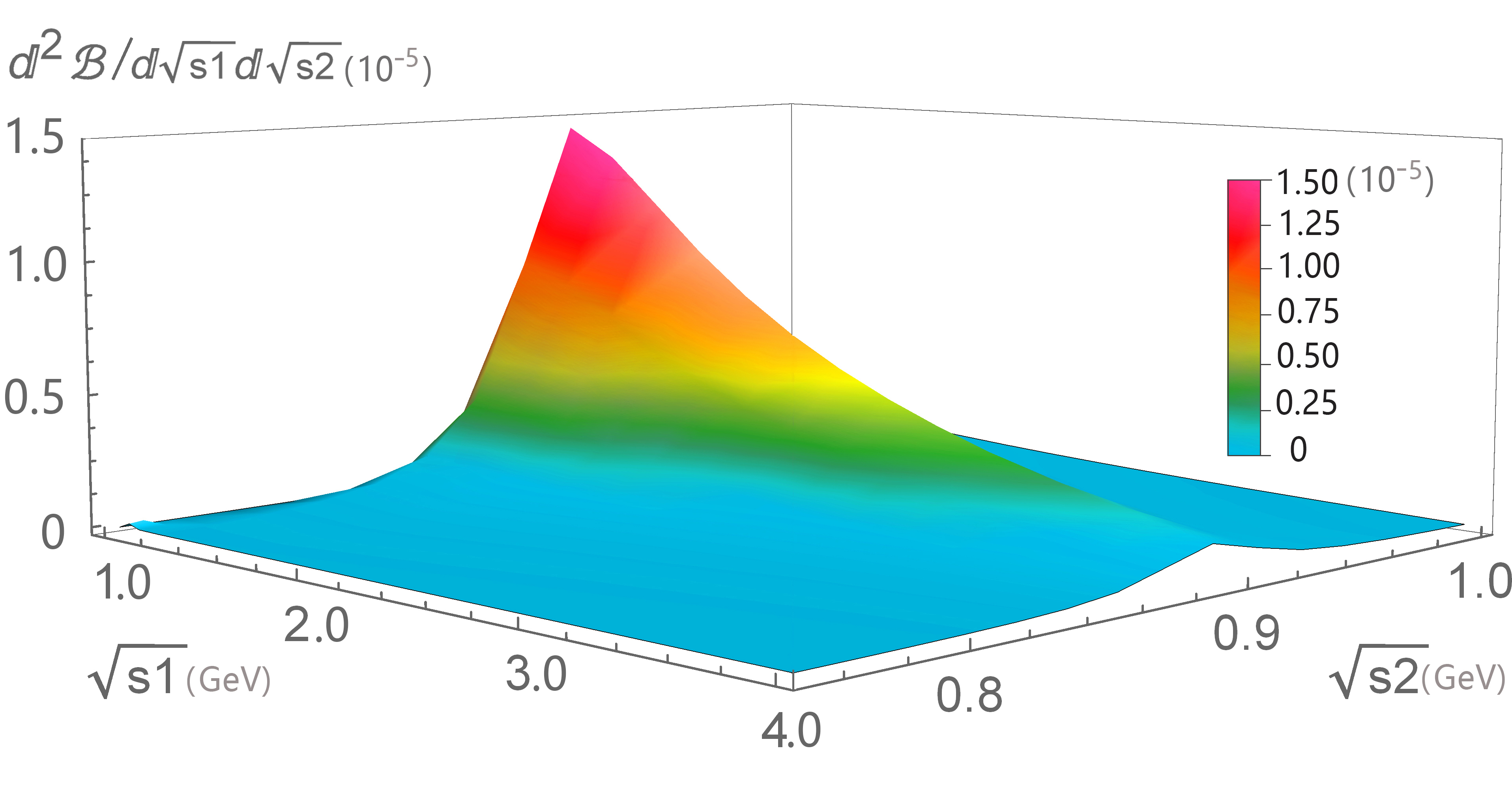
Figure 9: The differential branching ratio plot for the quasi-two-body decay process $\bar{B}_{s}\rightarrow[\phi(\rho^{0},\omega)\rightarrow K^{+}K^{-}][K^{*0}\rightarrow K^{+}\pi^{-}]$ .

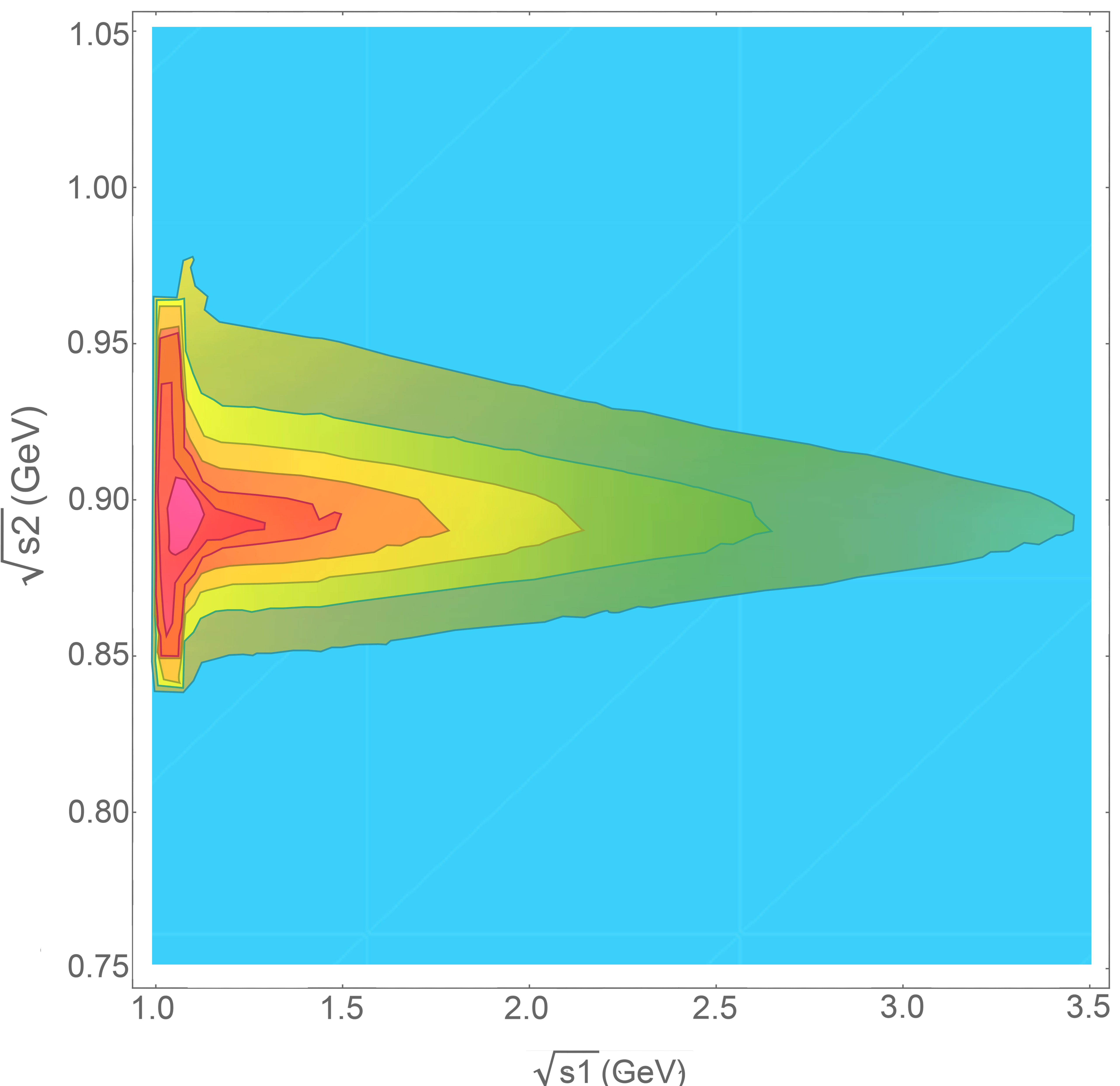
Figure 10: The plane mapping plot of the differential branching ratios for the decay process $\bar{B}_{s}\rightarrow[\phi(\rho^{0},\omega)\rightarrow K^{+}K^{-}][K^{*0}\rightarrow K^{+}\pi^{-}]$.

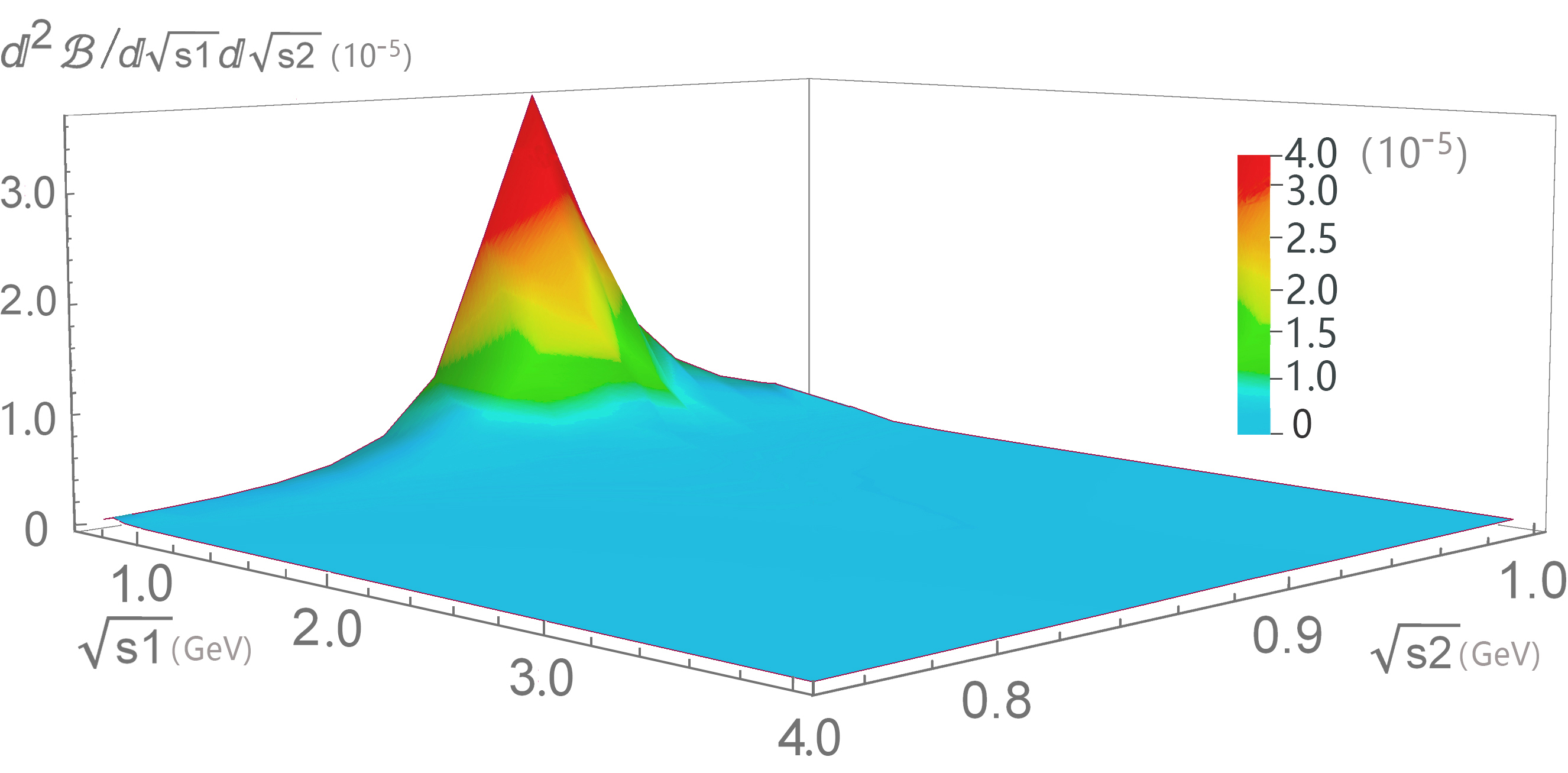
Figure 11: The differential branching ratio plot for the quasi-two-body decay process $\bar{B}_{s}\rightarrow[\rho^{0}(\omega,\phi)\rightarrow(\pi^{+}\pi^{-})][K^{*0}\rightarrow K^{+}\pi^{-}]$ .

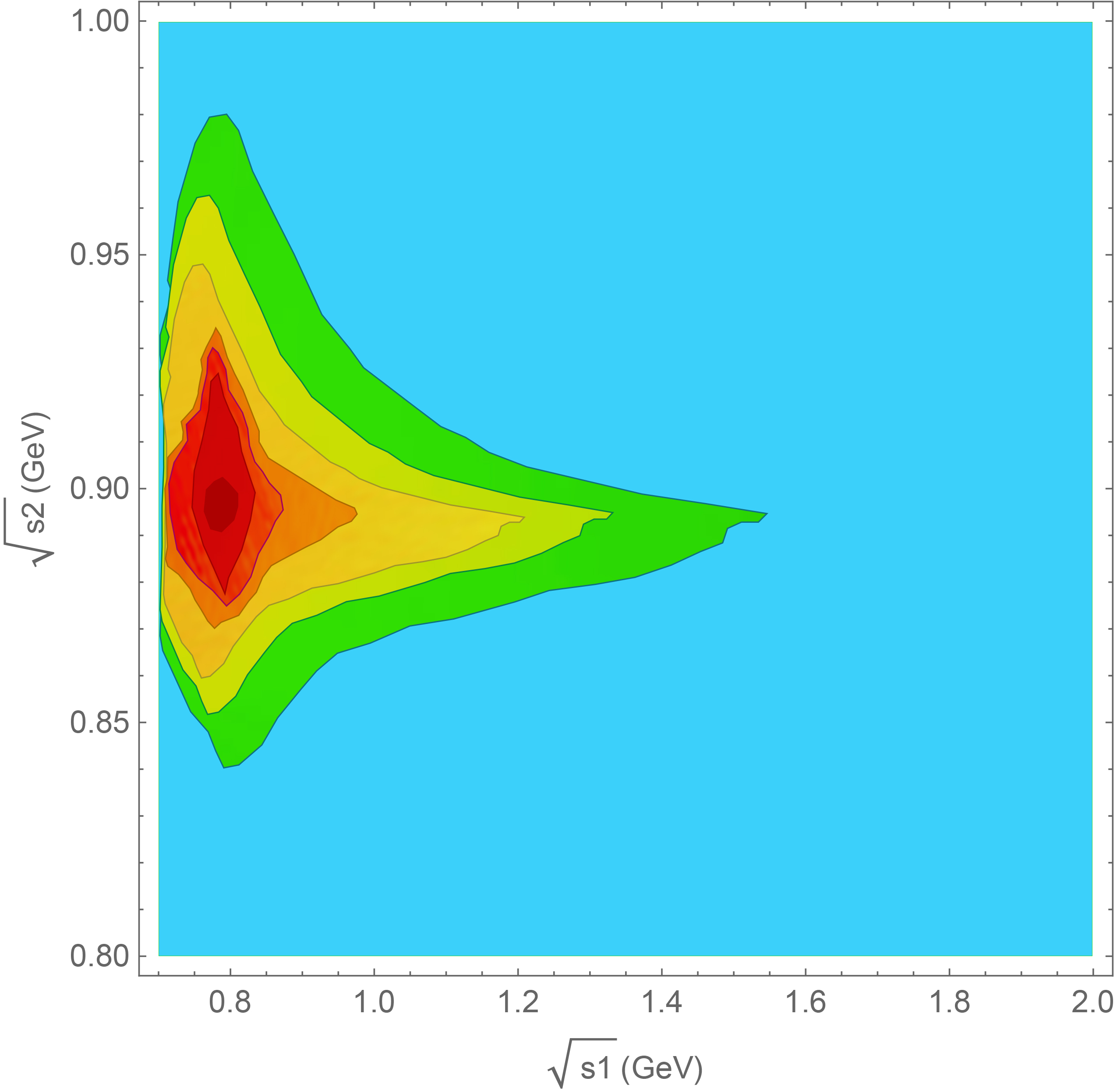
Figure 12: The plane mapping plot of the differential branching ratios for the decay process $\bar{B}_{s}\rightarrow[\rho^{0}(\omega,\phi)\rightarrow(\pi^{+}\pi^{-})][K^{*0}\rightarrow K^{+}\pi^{-}]$.

In Figs. 9 and 10, the differential branching ratios for the decay process $\bar{B}_{s}\rightarrow[\phi(\rho^{0},\omega)\rightarrow K^{+}K^{-}][K^{*0}\rightarrow K^{+}\pi^{-}]$ are illustrated. For the $\bar{B_{s}}\to(K^{+}K^{-})(K^{+}\pi^{-})$ decay, integration is performed within the peak regions, with the selected ranges being ${\sqrt{s_{1}}}$ from 0.99 to 1.2 GeV and ${\sqrt{s_{2}}}$ from 0.85 to 0.95 $GeV$. Similarly, in Figs. 11 and 12, the differential branching ratios for the decay process $\bar{B}_{s}\rightarrow[\rho^{0}(\omega,\phi)\rightarrow(\pi^{+}\pi^{-})][K^{*0}\rightarrow K^{+}\pi^{-}]$ are shown. For the $\bar{B_{s}}\to(\pi^{+}\pi^{-})(K^{+}\pi^{-})$ decay, integration is also conducted within the peak regions, with the chosen ranges being ${\sqrt{s_{1}}}$ from 0.70 to 1.10 $GeV$ and ${\sqrt{s_{2}}}$ from 0.85 to 0.95 $GeV$.

Table 5: Polarization fractions $\bar{B}_{s}\rightarrow{(K^{+}K^{-})(K^{+}\pi^{-})}$ and $\bar{B}_{s}\rightarrow{(\pi^{+}\pi^{-})(K^{+}\pi^{-})}$ decay processes.

Decay Channel	Modes	$f_{0}(\%)$	$f_{\|}(\%)$	$f_{\perp}(\%)$	${\cal B}(10^{-6})$
$\bar{B_{s}}\to(K^{+}K^{-})(K^{+}\pi^{-})$	$\rho^{0}K^{*0}$	$46.65^{\pm 0.32}_{\pm 9.31}$	$27.50^{\pm 0.02}_{\pm 2.65}$	$25.84^{\pm 0.30}_{\pm 2.35}$	$0.063^{\pm 0.006}_{\pm 0.039}$
	$\omega K^{*0}$	$50.12^{\pm 2.99}_{\pm 8.66}$	$25.78^{\pm 1.57}_{\pm 3.84}$	$24.10^{\pm 1.43}_{\pm 6.82}$	$0.014^{\pm 0.002}_{\pm 0.015}$
	$\phi K^{*0}$	$78.22^{\pm 0.53}_{\pm 12.76}$	$11.54^{\pm 0.32}_{\pm 3.25}$	$10.23^{\pm 0.18}_{\pm 1.56}$	$1.49^{\pm 0.10}_{\pm 0.56}$
	$(\phi-\rho^{0})K^{*0}$	$77.43^{\pm 0.02}_{\pm 4.53}$	$11.29^{\pm 0.01}_{\pm 1.45}$	$11.28^{\pm 0.01}_{\pm 1.16}$	$1.51^{\pm 0.07}_{\pm 0.52}$
	$(\phi-\omega)K^{*0}$	$76.54^{\pm 0.08}_{\pm 6.26}$	$12.18^{\pm 0.03}_{\pm 2.01}$	$11.28^{\pm 0.05}_{\pm 1.12}$	$1.28^{\pm 0.07}_{\pm 0.57}$
	$(\rho^{0}-\omega)K^{*0}$	$59.25^{\pm 2.36}_{\pm 8.89}$	$25.27^{\pm 1.42}_{\pm 5.84}$	$15.48^{\pm 0.94}_{\pm 3.94}$	$0.092^{\pm 0.017}_{\pm 0.043}$
	$(\phi-\rho^{0}-\omega)K^{*0}$	$75.90^{\pm 0.07}_{\pm 9.02}$	$12.68^{\pm 0.03}_{\pm 6.57}$	$11.41^{\pm 0.05}_{\pm 3.56}$	$1.28^{\pm 0.07}_{\pm 0.57}$
$\bar{B_{s}}\to(\pi^{+}\pi^{-})(K^{+}\pi^{-})$	$\rho^{0}K^{*0}$	$46.64^{\pm 0.31}_{\pm 9.19}$	$27.51^{\pm 0.01}_{\pm 2.43}$	$28.84^{\pm 0.12}_{\pm 2.24}$	$0.25^{\pm 0.03}_{\pm 0.07}$
	$(\rho^{0}-\omega)K^{*0}$	$39.65^{\pm 1.96}_{\pm 12.80}$	$36.03^{\pm 1.31}_{\pm 10.92}$	$24.32^{\pm 0.65}_{\pm 8.54}$	$0.38^{\pm 0.11}_{\pm 0.19}$
	$(\rho^{0}-\phi)K^{*0}$	$46.65^{\pm 0.32}_{\pm 9.18}$	$27.50^{\pm 0.02}_{\pm 2.42}$	$25.85^{\pm 0.29}_{\pm 2.25}$	$0.25^{\pm 0.02}_{\pm 0.06}$
	$(\rho^{0}-\omega-\phi)K^{*0}$	$39.66^{\pm 0.023}_{\pm 12.82}$	$36.03^{\pm 1.31}_{\pm 10.93}$	$24.31^{\pm 0.36}_{\pm 8.52}$	$0.58^{\pm 0.01}_{\pm 0.11}$

In Table V, we present the polarization fractions and corresponding branching ratios for the four-body decays through various intermediate states. Subsequently, we analyze the central values of these results. The branching ratio for the decay process $\bar{B_{s}}\to\phi(\phi\to K^{+}K^{-})K^{*0}(K^{*0}\to K^{+}\pi^{-})$ is two orders of magnitude higher than that for the decay processes $\bar{B_{s}}\to\rho^{0}(\rho^{0}\to K^{+}K^{-})K^{*0}(K^{*0}\to K^{+}\pi^{-})$ and $\bar{B_{s}}\to\omega(\omega\to K^{+}K^{-})K^{*0}(K^{*0}\to K^{+}\pi^{-})$. However, the polarization fractions $f_{\|}(\%)$ and $f_{\perp}(\%)$ for the decay processes $\bar{B_{s}}\to\rho^{0}(\rho^{0}\to K^{+}K^{-})K^{*0}(K^{*0}\to K^{+}\pi^{-})$ and $\bar{B_{s}}\to\omega(\omega\to K^{+}K^{-})K^{*0}(K^{*0}\to K^{+}\pi^{-})$ are approximately 2.5 times higher than those for the decay process $\bar{B_{s}}\to\phi(\phi\to K^{+}K^{-})K^{*0}(K^{*0}\to K^{+}\pi^{-})$. Due to the $\rho^{0}-\omega$ mixing, the branching ratio for the decay process $\bar{B_{s}}\to\rho^{0}(\omega)(\rho^{0}(\omega)\to K^{+}K^{-})K^{*0}(K^{*0}\to K^{+}\pi^{-})$ changes significantly compared to the direct decay $\bar{B_{s}}\to\phi(\phi\to K^{+}K^{-})K^{*0}(K^{*0}\to K^{+}\pi^{-})$ as shown in Table V. Meanwhile, the $\rho^{0}-\omega$ mixing also affects the polarization fractions: the polarization fraction $f_{0}$ decreases from $78.22\%$ to $59.25\%$, while $f_{\|}$ increases from $11.54\%$ to $25.27\%$ and $f_{\perp}$ increases from $10.23\%$ to $15.84\%$ when comparing $\bar{B_{s}}\to(\rho^{0}-\omega\to K^{+}K^{-})K^{*0}(K^{*0}\to K^{+}\pi^{-})$ with $\bar{B_{s}}\to\phi(\phi\to K^{+}K^{-})K^{*0}(K^{*0}\to K^{+}\pi^{-})$. After incorporating the mixing mechanisms of $\rho^{0}-\omega$ and $\rho^{0}-\omega-\phi$, the branching ratio and the longitudinal polarization fraction $f_{\|}(\%)$ for the decay $\bar{B_{s}}\to\rho^{0}(\rho^{0}\to\pi^{+}\pi^{-})K^{*0}(K^{*0}\to K^{+}\pi^{-})$ increase slightly, while the transverse polarization fraction $f_{0}(\%)$ decreases slightly. In contrast, introducing the $\rho^{0}-\phi$ mixing mechanism has a negligible effect on both the branching ratio and the polarization fractions for this decay.

In the heavy quark limit, theoretical uncertainties arise from various sources, leading to ambiguity in the results. Specifically, the $1/m_{b}$ power correction introduces additional complexity that necessitates a thorough error analysis. In this study, the primary sources of error are as follows: First, uncertainties associated with the CKM matrix elements; Second, uncertainties stemming from hadronic interaction parameters, including form factors, decay constants, and meson wave functions.

VIII Summary and conclusion

In this work, we introduce the $\rho-\omega-\phi$ mesons mixing mechanism and study the CP violation, regional CP violation ($A^{\Omega}_{CP}$), polarization fractions, and branching ratios in the four-body decay processes of $\bar{B}_{s}\rightarrow(K^{+}K^{-})(K^{+}\pi^{-})$ and $\bar{B}_{s}\rightarrow(\pi^{+}\pi^{-})(K^{+}\pi^{-})$ under the PQCD approach. The interference effects arising from the mixing of $\rho$, $\omega$, and $\phi$ mesons lead to more pronounced CP violation phenomena compared to direct decay processes. ${A}^{\Omega}_{CP}$ is quantified by integrating over phase space, and distinct CP violation is observed for different mixing intermediate states when the invariant mass of the $K^{+}K^{-}(\pi^{+}\pi^{-})$ pair is within specific ranges. When the invariant masses of $K^{+}K^{-}$ pair and $\pi^{+}\pi^{-}$ pair are in the resonance region, the CP violation can be detected experimentally by reconstructing $\rho$, $\omega$ and $\phi$ mesons. This study may provide some reference for the future detection and research of the LHCb experiment.

In 2010, the Large Hadron Collider (LHC) at CERN successfully carried out proton-proton collisions at $7$ TeV. The LHC is designed with a center-of-mass energy of $14$ TeV and a luminosity of $L=10^{34}cm^{-2}s^{-1}$. The production cross-section of $b\bar{b}$ at the LHC is anticipated to be $0.5mb$, yielding approximately $0.5\times 10^{12}$ bottom events annually QuarkoniumWorkingGroup:2004kpm . The LHCb experiment, leveraging these events, focuses on studying CP violation and rare decays within the $b$ hadron system. During Runs 1 and 2, LHCb amassed substantial data, while ATLAS and CMS gathered $5fb^{-1}$, $20fb^{-1}$, and $150fb^{-14}$ at $\sqrt{s}=7$ TeV, $8$ TeV, and $13$ TeV, respectively. The High-Luminosity Large Hadron Collider (HL-LHC) and its potential upgrade to the High-Energy Large Hadron Collider (HE-LHC), a $27$ TeV proton-proton collider, are poised to further advance flavor physics research. The experimental sensitivity of the HL-LHC is expected to markedly improve, with ATLAS and CMS planning to record $3000fb^{-1}$ of data and LHCb’s Upgrade II aiming to capture $300fb^{-1}$ Cerri:2018ypt . These datasets will offer new opportunities for the study of CP violation phenomena.

References

• (1) N. Cabibbo, Phys. Rev. Lett. 10,531 (1963).
• (2) Z. H. Zhang, X. H. Guo and Y. D. Yang, Phys. Rev. D 87, 076007 (2013).
• (3) S. T. Li and G. Lü, Phys. Rev. D 99, 116009 (2019).
• (4) D. S. Shi, G. Lü, Y. L. Zhao, Na-Wang and X. H. Guo, Eur. Phys. J. C 83, 345 (2023).
• (5) G. Lü, Y. L. Zhao, L. C. Liu and X. H. Guo, Chin. Phys. C 46, 113101 (2022).
• (6) J. H. Christenson, J. W. Cronin, V. L. Fitch and R. Turlay, Phys. Rev. Lett. 13, 138-140 (1964).
• (7) A. Alavi-Harati et al. [KTeV], Phys. Rev. Lett.84, 408 (2000).
• (8) K. Abe et al. [Belle], Phys. Rev. Lett. 87, 091802 (2001).
• (9) B. Aubert et al. [BaBar], Phys. Rev. D. 65, 051101 (2002).
• (10) R. Aaij et al. [LHCb], LHCb-CONF-2012-018 (2012).
• (11) R. Aaij et al. [LHCb], LHCb-CONF-2012-028 (2012).
• (12) C. L. Hsu et al. [Belle], Phys. Rev. D 96, 031101 (2017).
• (13) R. Aaij et al. [LHCb], Phys. Rev. Lett. 131, 171802 (2023).
• (14) I. Bediaga, T. Frederico and O. Lourenço, Phys. Rev. D 89, 094013 (2014).
• (15) H. Y. Cheng, C. K. Chua and Z. Q. Zhang, Phys. Rev. D 94, 094015 (2016).
• (16) R. Klein, T. Mannel, J. Virto and K. K. Vos, JHEP 10, 117 (2017).
• (17) Y. Li, A. J. Ma, Z. Rui, W. F. Wang and Z. J. Xiao, Phys. Rev. D 98, 056019 (2018).
• (18) G. Lü, Y. T. Wang and Q. Q. Zhi, Phys. Rev. D 98, 013004 (2018).
• (19) A. J. Ma, W. F. Wang, Y. Li and Z. J. Xiao, Eur. Phys. J. C 79, 539 (2019)
• (20) R. Aaij et al. [LHCb], Phys. Rev. Lett. 123, 231802 (2019).
• (21) R. Aaij et al. [LHCb], Phys. Rev. Lett. 124, 031801 (2020).
• (22) D. C. Yan, Z. Rui, Z. J. Xiao and Y. Li, Phys. Rev. D 105, 093001 (2022).
• (23) H. Q. Liang and X. Q. Yu, Phys. Rev. D 105, 096018 (2022).
• (24) M. Bander, D. Silverman and A. Soni, Phys. Rev. Lett. 43, 242 (1979).
• (25) C. D. Lu, K. Ukai and M. Z. Yang, Phys. Rev. D 63, 074009 (2001).
• (26) Y. Y. Keum, H. N. Li and A. I. Sanda, Phys. Lett. B 504, 6 (2001).
• (27) Y. Y. Keum, H. N. Li and A. I. Sanda, Phys. Rev. D 63, 054008 (2001).
• (28) Z. J. Xiao, D. Q. Guo and X. f. Chen, Phys. Rev. D 75, 014018 (2007).
• (29) C. C. Zhang and G. Lü, Phys. Rev. D 111, 033001 (2025).
• (30) Z. T. Zou, Y. Li and X. Liu, Eur. Phys. J. C 80, 517 (2020).
• (31) J. Hua, H. N. Li, C. D. Lu, W. Wang and Z. P. Xing, Phys. Rev. D 104, 016025 (2021).
• (32) C. H. V. Chang and H. N. Li, Phys. Rev. D 55, 5577 (1997).
• (33) T. W. Yeh and H. N. Li, Phys. Rev. D 56, 1615 (1997).
• (34) G. P. Lepage and S. J. Brodsky, Phys. Rev. D 22, 2157 (1980).
• (35) J. Botts and G. F. Sterman,Nucl. Phys. B 325, 62 (1989).
• (36) A. Ali, G. Kramer, Y. Li, C. D. Lu, Y. L. Shen, W. Wang and Y. M. Wang, Phys. Rev. D 76, 074018 (2007).
• (37) H. Y. Cheng, C. W. Chiang and C. K. Chua, Phys. Rev. D 103, 036017 (2021).
• (38) H. Y. Cheng, C. W. Chiang and C. K. Chua, Phys. Lett. B 813, 136058 (2021).
• (39) Y. Nambu, Phys. Rev. 106, 1366 (1957).
• (40) N. M. Kroll, T. D. Lee and B. Zumino, Phys. Rev. 157, 1376 (1967).
• (41) P. M. Ivanov, L. M. Kurdadze, M. Y. Lelchuk, V. A. Sidorov, et al., Phys. Lett. B 107, 297 (1981).
• (42) M. N. Achasov, V. M. Aulchenko, A. Y. Barnyakov, M. Y. Barnyakov, et al. Phys. Rev. D 94, 112006 (2016).
• (43) H. B. O,Connell, B. C. Pearce, A. W. Thomas and A. G. Williams, Prog. Part. Nucl. Phys.39, 201 (1997).
• (44) G. Lü, Y. L. Zhao, L. C. Liu and X. H. Guo, Chin. Phys. C 46, no.11, 113101 (2022).
• (45) G. Lü, C. C. Zhang, Y. L. Zhao and L. Y. Zhang, Chin. Phys. C 48, 013103 (2024)
• (46) C. E. Wolfe and K. Maltman, Phys. Rev. D 80, 114024 (2009).
• (47) C. E. Wolfe and K. Maltman, Phys. Rev. D 83, 077301 (2011).
• (48) M. N. Achasov, V. M. Aulchenko, A. V. Berdyugin, A. V. Bozhenok, et al., Nucl. Phys. B 569, 158 (2000)
• (49) A. Pais and S. B. Treiman, Phys. Rev. 168, 1858 (1968).
• (50) G. L. Kane, K. Stowe and W. B. Rolnick, Nucl. Phys. B 152, 390 (1979).
• (51) C. L. Y. Lee, M. Lu and M. B. Wise, Phys. Rev. D 46, 5040 (1992).
• (52) G. Kramer and W. F. Palmer, Phys. Lett. B 298, 437 (1993).
• (53) A. G. Grozin, Sov. J. Nucl. Phys. 38 , 289 (1983).
• (54) A. G. Grozin, Theor. Math. Phys. 69 , 1109 (1986).
• (55) D. Müller, D. Robaschik, B. Geyer, F. M. Dittes and J. Hořejši, Fortsch. Phys. 42, 101-141 (1994).
• (56) M. Diehl, T. Gousset, B. Pire and O. Teryaev, Phys. Rev. Lett. 81, 1782 (1998).
• (57) M. Diehl, T. Gousset and B. Pire, Phys. Rev. D 62, 073014 (2000).
• (58) P. Hagler, B. Pire, L. Szymanowski and O. V. Teryaev, Eur. Phys. J. C 26, 261 (2002).
• (59) Y. K. Hsiao and C. Q. Geng, Phys. Lett. B 770, 348 (2017).
• (60) C. H. Chen, Y. Y. Keum and H. N. Li, Phys. Rev. D 66, 054013 (2002).
• (61) C. D. Lu, Y. l. Shen and J. Zhu, Eur. Phys. J. C 41, 311-317 (2005).
• (62) H. N. Li and S. Mishima, Phys. Rev. D 71, 054025 (2005).
• (63) H. W. Huang, C. D. Lu, T. Morii, Y. L. Shen, G. Song and Jin-Zhu, Phys. Rev. D 73, 014011 (2006).
• (64) Y. H. Chen, H. Y. Cheng, B. Tseng and K. C. Yang, Phys. Rev. D 60, 094014 (1999).
• (65) C. Bruch, A. Khodjamirian and J. H. Kuhn, Eur. Phys. J. C 39, 41 (2005).
• (66) H. Y. Cheng and C. K. Chua, Phys. Rev. D 102, 053006 (2020).
• (67) H. N. Li and S. Mishima, Phys. Rev. D 74, 094020 (2006).
• (68) R. Aaij et al. [LHCb], Phys. Rev. D 98, 072006 (2018).
• (69) R. Aaij et al. [LHCb], Phys. Rev. Lett. 122, 152002 (2019).
• (70) I. Bezshyiko et al. [LHCb], Phys. Rev. Lett. 132, 051802 (2024).
• (71) S. H. Kyeong et al. [Belle], Phys. Rev. D 80, 051103 (2009).
• (72) C. C. Chiang et al. [Belle], Phys. Rev. D 81, 071101 (2010).
• (73) B. Aubert et al. [BaBar], Phys. Rev. Lett. 100, 081801 (2008).
• (74) B. Aubert et al. [BaBar], Phys. Rev. Lett. 101, 201801 (2008).
• (75) H. Y. Cheng and C. K. Chua, Phys. Rev. D 102, 053006 (2020).
• (76) M. Kobayashi and T. Maskawa, Prog. Theor. Phys. 49, 652 (1973).
• (77) L. Wolfenstein, Phys. Rev. Lett. 51, 1945 (1983).
• (78) S. Navas et al. [Particle Data Group], Phys. Rev. D 110, 030001 (2024).
• (79) N. Brambilla et al. [Quarkonium Working Group], CERN-2005-005 (2005).
• (80) A. Cerri, V. V. Gligorov, S. Malvezzi, et al. CERN Yellow Rep. Monogr. 7, 867 (2019).