A Composable Game-Theoretic Framework for Blockchains

Abstract.

Blockchains rely on economic incentives to ensure secure and decentralised operation, making incentive compatibility a core design concern. However, protocols are rarely deployed in isolation. Applications interact with the underlying consensus and network layers, and multiple protocols may run concurrently on the same chain. These interactions give rise to complex incentive dynamics that traditional, isolated analyses often fail to capture.

We propose the first compositional game-theoretic framework for blockchain protocols. Our model represents blockchain protocols as interacting games across layers—application, network, and consensus. It enables formal reasoning about incentive compatibility under composition by introducing two key abstractions: the cross-layer game, which models how strategies in one layer influence others, and cross-application composition, which captures how application protocols interact concurrently through shared infrastructure.

We illustrate our framework through case studies on HTLCs, Layer-2 protocols, and MEV, showing how compositional analysis reveals subtle incentive vulnerabilities and supports modular security proofs.

1. Introduction

Blockchains currently secure more than $3 trillion in digital assets. As most operate in an open, permissionless fashion, such as Bitcoin and Ethereum, their security fundamentally relies on financial incentives. That is, participants invest resources, whether computational power or cryptocurrency holdings, in exchange for rewards such as block rewards and transaction fees.

This incentive-driven security model supports a broader ecosystem commonly referred to as Web3—a decentralised digital environment where applications operate on distributed networks rather than being governed by centralised entities. Web3 is composed of multiple interdependent layers, each fulfilling distinct roles. At its core, the blockchain (or consensus) layer is responsible for ordering transactions in a trustless manner. On top of it operates the application layer, which includes decentralised applications (dApps) and Layer 2 (L2) solutions designed to enhance functionality, efficiency, and scalability of the underlying blockchain layer. Underpinning these layers is the network layer, which facilitates secure and reliable communication among geographically distributed participants.

These layers do not operate in isolation. Their interdependence gives rise to complex security dependencies that fall outside the scope of traditional game-theoretic models, which typically focus on a single layer while abstracting away the rest. In particular, incentives leak across layers, introducing subtle but critical vulnerabilities. Notable examples of such cross-layer issues include timelock bribing attacks (Nadahalli et al., 2021; Avarikioti and Litos, 2022) and Maximal Extractable Value (MEV) exploits (Daian et al., 2020). In timelock bribing attacks, adversaries at the application layer bribe validators to censor transactions, allowing them to extract funds from protocols relying on time-based smart contracts. MEV exploits, in contrast, arise from validators (or external actors) observing pending transactions and manipulating their inclusion on-chain–for instance, via frontrunning, backrunning, or sandwich attacks (Zhou et al., 2023). While timelock bribing constitutes an explicit security breach, MEV exploits reflect an emergent consequence of misaligned incentives between the network and consensus layers. Both cases underscore the limitations of layer-specific security models and highlight the need for a compositional game-theoretic security framework; one that captures the incentive dynamics spanning multiple layers and supports the design of economically secure blockchain protocols.

Nevertheless, existing analyses largely fail to address this need. Prior works either do not account for rational behaviour, remaining rooted in cryptographic models that assume participants are honest or Byzantine, e.g., (Garay et al., 2024; Kiayias et al., 2017; Gilad et al., 2017; Daian et al., 2019; Yin et al., 2019), or adopt monolithic rational models that abstract away cross-layer interactions, e.g., (Garay et al., 2013; Badertscher et al., 2018; Kiayias et al., 2016; Aiyer et al., 2005; Pass and Shi, 2017; Avarikioti et al., 2020b, 2024). As a result, none of these approaches offer a general, composable framework capable of reasoning about cross-layer incentive dynamics or the concurrent execution of multiple application protocols on a shared blockchain infrastructure.

1.1. Our Contributions

This work addresses this gap by introducing a composable game-theoretic framework for blockchains that enables formal reasoning about protocol security across multiple layers of the blockchain stack. To this end, we characterise and formalise the distinct layers of a blockchain ecosystem—the application, network, and consensus layers—alongside the interfaces that govern their interactions.

We first define the blockchain game, which models the strategic behaviour of miners or validators in response to a set of fee-paying transactions. We then define the application game, which captures the actions of protocol participants operating an application-layer protocol and whose outcome is a set of transaction triples (each consisting of a transaction, a fee, and a timestamp) intended for submission to the blockchain. Finally, we introduce the network game, a novel intermediary layer that models how these transactions are disseminated to the consensus layer. This is the layer where phenomena such as Maximal Extractable Value (MEV) emerge, as it governs the visibility and timing of transactions across the system.

To reason about incentive security in such settings, we introduce a rigorous notion of game-theoretically secure protocols. Informally, we require that the expected utility of protocol participants does not increase when the protocol is executed in a composed setting—interacting with the blockchain game, the network game, and other application games—compared to when it is executed in isolation. At the core of our framework are two new constructs: the cross-layer game, which integrates the application, network, and blockchain layers to capture their strategic interplay, and cross-application composition, which enables reasoning about the concurrent execution of multiple protocols on a shared blockchain infrastructure.

We demonstrate the expressiveness and generality of our framework through a number of illustrative applications. First, we model and analyse the composition of Hashed Timelock Contracts (HTLCs) across multiple payment channels, identifying those parameter regimes under which compositional security holds in the presence of rational participants. Second, we revisit, using our framework, a recent payment channel protocol (Aumayr et al., 2024) and derive tighter incentive bounds by leveraging a more expressive blockchain model. Finally, we illustrate how even a simple broadcast network model can, when composed with an application game, lead to rational miners deviating from consensus to exploit MEV opportunities. This showcases how our framework can surface emergent vulnerabilities that layer-specific analyses fail to capture.

Beyond these detailed examples, we outline a broader class of settings that our framework naturally captures. These include interactions between decentralized exchanges and oracles, cross-chain protocols such as atomic swaps, and multi-layer incentive mechanisms like proposer-builder separation (PBS). While not formalised as case studies, these examples underscore the versatility and broader applicability of our framework for reasoning about complex, concurrent protocols within modern blockchain ecosystems.

Summary of Contributions.

Our contributions are as follows:

• We develop the first composable game-theoretic framework for blockchain ecosystems, capturing incentive interactions across application, network, and consensus layers.

• We formalise three core games—the blockchain game, the application game, and the network game—and define their composition.

• We introduce the notions of cross-layer games and of cross-application composition to enable compositional reasoning about protocol security under rational participants.

• We apply our framework to multiple case studies showcasing its ability to capture incentive dynamics, expose vulnerabilities, and improve security through composition. We further outline broader applications to demonstrate the framework’s potential to model complex settings such as cross-application, cross-chain, and multi-layer interactions.

Paper Organisation

Section 1.2 reviews prior work. In Section 2, we introduce our framework by translating protocols into formal games, which allows us to define incentive compatibility in a composable setting. Section 3 then formalises the composition of these games and identifies conditions under which incentive compatibility is preserved. To illustrate the applicability of our framework, Section 4 presents several representative case studies. Finally, Section 5 discusses the framework’s limitations and outlines directions for future research.

1.2. Related Work

Layer-specific models.

A large body of work studies incentive mechanisms within isolated layers of the blockchain stack. At the consensus layer, researchers have analysed block rewards (Eyal and Sirer, 2018; Budish et al., 2024; Chen et al., 2019) and transaction fee mechanisms (Bahrani et al., 2024b, a; Roughgarden, 2024). Other works model consensus dynamics using rational agents (Abraham et al., 2013; Aiyer et al., 2005; Amoussou-Guenou et al., 2019; Kiayias et al., 2016; Bentov et al., 2021; Kiayias and Stouka, 2021; Liao and Katz, 2017; Winzer et al., 2019; Liu et al., 2019; Pass and Shi, 2017; Budish et al., 2024). Similarly, other works restrict their analysis on the network layer, e.g. (Babaioff et al., 2012). Several works conduct a rational analysis on the application layer, either targeting specific applications like auctions (Chitra et al., 2023) or off-chain systems like payment channels (Avarikioti et al., 2020a, 2024, b; Rain et al., 2023; Aumayr et al., 2025). However, these results assume fixed behaviour from other layers and do not account for strategic interactions across layers or with other applications. In contrast, our framework explicitly models such cross-layer and cross-application dependencies.

Monolithic protocol analyses. Some works jointly analyse protocol layers, especially in Layer-2 constructions where application behaviour and miner incentives interact (Tsabary et al., 2021; Wadhwa et al., 2022; Aumayr et al., 2024; Avarikioti and Litos, 2022; Avarikioti et al., 2021, 2025; Doe et al., 2023). For instance, (Tsabary et al., 2021; Wadhwa et al., 2022) model how rational miners affect the execution of HTLCs. However, these analyses are monolithic, capturing the entire system in a single game. This limits extensibility and compositional reasoning: security properties must be re-derived from scratch for each new protocol interaction. Our approach instead defines modular game components with formally specified interfaces, allowing reuse and composition across protocols.

MEV and dynamic incentives. Daian et al. (Daian et al., 2020) introduced the concept of Maximal Extractable Value (MEV), showing how application-level transactions influence miner strategies. Follow-up work has explored incentive-aligned auction designs and mitigation techniques (Doe et al., 2023), but analyses remain tightly coupled to specific systems and do not generalise to arbitrary protocol interactions. Our framework generalises MEV through the network game, an abstraction that sits between the application and blockchain layers. This allows for systematic reasoning about its impact across a wide range of protocol designs.

Cross-application and cross-layer security. More closely related to our approach is the work by Zappalà et al. (2021), which aims to formalise secure protocol composition. Unlike our framework, theirs assumes independence between subgames rather than deriving it, limiting applicability for systems with interdependent protocols. For example, in their analysis of the Lightning Network (Poon and Dryja, 2016), they treat HTLCs as independent if all transactions are posted on time, thereby sidestepping strategic deviations. Their approach defines security conditions statically and does not account for the dynamic strategic behaviours that can arise during execution. In contrast, our framework handles compositional reasoning even when games are not independent, enabling the analysis of incentive-driven interactions such as adversarial timing or MEV extraction across concurrent protocols.

Compositional game theory. Our work is inspired by compositional game theory (Ghani et al., 2018), which uses category-theoretic tools to model complex systems as compositions of modular components called open games. While this approach offers a powerful and elegant abstraction, it remains largely theoretical and lacks concrete results about how strategic behaviour composes. Moreover, it does not address domain-specific settings like blockchains, where incentives are shaped by structured interfaces such as transaction propagation and fee mechanisms. In contrast, our framework instantiates these compositional principles in the blockchain setting, leveraging its layered architecture to define explicit interfaces and enabling formal reasoning about incentive compatibility and strategic behaviour across interdependent protocols. This enables us to derive concrete results that would be challenging to obtain using the abstract approach of Ghani et al. (2018).

Rational protocol design and simulation-based models. Our approach also differs fundamentally from Rational Protocol Design (RPD)(Garay et al., 2013; Badertscher et al., 2018), which models security as a Stackelberg game between a protocol designer and an attacker, with utilities defined via ideal functionalities in the simulation paradigm. While RPD inherits compositionality from the Universal Composability (UC) framework(Canetti, 2001), this form of composition corresponds to subroutine replacement and does not address how strategic behaviour composes across protocols. In contrast, our framework models composition at the level of incentives and strategic interaction, allowing us to reason about equilibrium properties in composed games. For instance, RPD can capture the behaviour of a single validator extracting MEV in a fixed environment, but it lacks the tools to analyse how MEV opportunities arise from the strategic interplay of multiple protocols, such as DEX arbitrage, oracle manipulation, or searcher-builder auctions, operating concurrently over shared infrastructure. Our framework, by explicitly modelling the application, network, and consensus layers, supports such analyses and enables formal reasoning about incentive alignment in systems where protocols interact dynamically and adversarially.

Automated tools. Recent automated tools for reasoning about rational security, such as CheckMate (Brugger et al., 2023), focus on verifying strategic properties in isolated protocols using symbolic game representations. These tools provide valuable automation but do not model layered architectures or inter-protocol interactions. In contrast, our framework is designed to analyse composed systems spanning multiple layers and concurrent applications.

This work. While prior works offer valuable insights into rational security, they either focus narrowly on isolated components, assume idealised independence between interacting parts, lack a modular framework for capturing the dynamic nature of incentive interactions across protocols and layers, or are too abstract to yield concrete results in blockchain settings. Our framework fills this gap by enabling modular, game-theoretic analysis of blockchain systems as they are deployed in practice.

2. Model

Our framework aims to support a broad class of protocols operating atop a common blockchain infrastructure. We consider three distinct layers: a network layer, composed of nodes that communicate over a peer-to-peer network; a consensus layer, which establishes an ordered sequence of transactions; and an application layer, that captures the internal logic of decentralised applications. Our framework models each of these layers separately and formalises their interfaces. This enables us to reason about the composition of the different layers and consequently study the game-theoretic security properties of protocols operating within a blockchain ecosystem in a modular way.

Game-theoretic security concerns the behaviour of rational players who act to maximise their utility, typically measured in cryptocurrency holdings. A protocol is said to be incentive-compatible (IC) if following its prescribed behaviour yields the highest expected utility for all participants, making deviation unprofitable.

Participants behave rationally if they act to maximise their utility. The utility function can be defined to model different behaviours. For instance, participants may always follow the protocol, which can be modelled by assigning infinite utility when they comply and zero otherwise. Alternatively, adversarial participants may derive utility from minimising another participant’s utility. In the following, we make the natural assumption that everyone tries to maximise their cryptocurrency holdings, but we stress that our framework can accommodate other utility functions as well.

We assume that participants can collude, meaning they can coordinate strategies and aggregate their utilities. Colluding participants effectively merge into a single entity capable of executing joint actions. They can also freely share any information they possess. Conversely, non-colluding participants can only communicate through the blockchain. We will formally define collusion and information-sharing later in this work.

Remark 2.1.

Incentive compatibility does not assess the quality of a protocol’s design. A flawed protocol – such as one that destroys half of all participants’ funds – could still be IC if rational participants adhere to its prescribed actions. While such protocols may be impractical, our focus is solely on whether rational agents will follow the protocol once they choose to participate.

The cryptocurrency holdings of all players (which they try to maximise) are determined by the state of the blockchain. This state can be updated by players broadcasting transactions over the network. The role of the blockchain is to create an ordered sequence of transactions. We will denote by $\mathscr{X}$ the set of all transactions that could be made within the blockchain ecosystem, and denote by $\Omega$ the set of all orderings of (a subset of) transactions in $\mathscr{X}$. We abstract the behaviour of the blockchain as the following mapping.

Definition 2.2.

We define a blockchain behaviour $\beta:\mathscr{X}\to\Omega$ as a function which has as input a set $X\in\mathscr{X}$ of transactions, and outputs a sequence $(A_{t})_{t\geq 0}$ of blocks of transactions, where for each $t\geq 0$, $A_{t}\subseteq X$ is a sequence of transactions. We call $A_{t}$ a block and a specific instance of the output a (blockchain) ordering.

Remark 2.3.

Our definition of a blockchain behaviour is as abstract as possible, in order to accommodate for the widest range of existing blockchain systems. It should be noted that the transactions in $\mathscr{X}$ are defined to implicitly contain all the information necessary for the function $\beta$ to determine an ordering. For example, a transaction in $\mathscr{X}$ may implicitly define a transaction fee, as well as a time at which its existence becomes known to $\beta$. Explicitly keeping track of these fee and time attributes will in fact be crucial for our framework.

This ordered sequence of transactions can then be executed according to a specific set of rules, which leads to an update in the state. Concretely, given an ordering $(A_{t})_{t\geq 0}\in\Omega$, the set of execution rules defines for each participant $i$ its balance in the blockchain ecosystem. This can be abstracted with an execution function $\omega_{i}:\Omega\to\mathbb{R}$, which for a given ordering returns the balance of a given participant $i$.

2.1. The Blockchain Game

We are interested in turning a blockchain behaviour into an object, which we can reason with game-theoretically. After all, the ordering that comes out upon input of a set of transactions is potentially determined by decisions made by rational actors, who try to maximise a given utility. These actors could be miners in a Proof-of-Work blockchain, or validators in a Proof-of-Stake blockchain.

To this end, we introduce the blockchain game. This is not a game in the traditional game-theoretic sense due to the lack of a utility function. To keep our framework as modular as possible, we refrain from defining the utility function as part of this blockchain game, but introduce it only in Section 3.1. The players in this game are the miners or validators. Upon input of a set of transactions, their decisions will lead to a certain blockchain ordering. In our framework, we explicitly mention two attributes alongside each transaction: a posting time and a transaction fee. This does not contradict Definition 2.2, as this information is considered to be already present in the transaction, we just explicitly keep track of it. Intuitively, the posting time determines when a miner/validator learns about the existence of a transaction, and the transaction fee determines what utility the miner/validator receives by including that transaction in the ordering. By explicitly stating the posting time and transaction fee, we extract from the transaction the information that players in the blockchain game need to make decisions. We therefore speak of transaction triples. These are tuples $(x,t,f)$, with $x$ a transaction, $t\in\mathbb{N}_{0}$ the posting time of that transaction, and $f\in\mathbb{R}_{\geq 0}$ the transaction fee. For a given set $X$ of transactions, we denote by $\mathscr{Y}(X)$ the set of all sets of transaction triples of $X$, i.e., $\mathscr{Y}(X)=\mathscr{P}\quantity(\quantity{(x,t,f):x\in X,t\in\mathbb{N}_{0},f\in\mathbb{R}_{\geq 0}})$.

The blockchain game thus takes as input a set of transaction triples $Y$ for some set of transactions $X$. The players in this game then all decide on a strategy, which results in an ordering $b\in\mathscr{O}_{M}(Y)$ of the transactions present in $Y$, i.e., the transactions in $X_{Y}=\quantity{x\in X:\exists t\in\mathbb{N}_{0},\exists f\in\mathbb{R}_{\geq 0}:(x,t,f)\in Y}$. We denote here by $\mathscr{O}_{M}(Y)\subseteq\Omega$ the set of all possible orderings from an input set $Y$ of transaction triples for a given set of blockchain game players $M$. Recall that $\Omega$ is the set of all possible orderings. More correctly, given $Y$, the strategies of the players give a strategy profile, which results in a probability measure on $\mathscr{O}_{M}(Y)$, as there might still be an element of randomness involved in determining the ordering.

Definition 2.4 (Blockchain Game).

Let $Y\in\mathscr{Y}(X)$ be a set of transaction triples for some set $X$ of transactions. Denote by $X_{Y}=\quantity{x\in X:\exists t\in\mathbb{N}_{0},\exists f\in\mathbb{R}_{\geq 0}:(x,t,f)\in Y}$ the set of transactions present in $Y$. The blockchain game $\mathcal{B}_{Y}$ induced by $Y$ is a tuple $(M,Y,\Sigma_{bg},\pi_{bg})$, where:

• $M$ is the set of miners/validators, which are the players of the blockchain game, together with their respective hashrates (for miners) or stakes (for validators).

• $\Sigma_{bg}$ is the set of strategy profiles. For any $(x,t,f)\in Y$, players of the blockchain game only become aware of the transaction $x$ and its fee $f$ at time $t$.

• $\pi_{bg}:\Sigma_{bg}\to\mathscr{D}(\mathscr{O}_{M}(Y))$ is the ordering function, which maps every strategy profile in $\Sigma_{bg}$ to a probability measure on $\mathscr{O}_{M}(Y)$.

It will be useful later to keep track of which player in $M$ will receive the transaction fee for a specific transaction by introducing a dedicated function, which we call the fee function.

Definition 2.5 (Fee function).

For a set of miners $M$ and a set of transaction triples $Y$, we define the fee function $\phi=(\phi_{j})_{j\in M}$, where for each $j\in M$, $\phi_{j}:\mathscr{O}_{M}(Y)\to\mathscr{P}(Y)$ maps each ordering to the set of transaction triples for which $j$ receives the transaction fees.

It is far from trivial to capture all of the complexity of a blockchain behaviour in the format of a blockchain game. Simplifications are therefore necessary. For now, we assume a simple blockchain behaviour with a random leader selection, in the spirit of Bitcoin, where each miner can decide on which transactions to include and at what time, but always builds on the same chain and does not withhold valid blocks that it found, as in selfish mining (Eyal and Sirer, 2018). We also assume that the transactions we input into this game are the only fee-paying ones, so there are no other ways, such as other transactions or block rewards, by which the miners can gain funds. We call this blockchain game the Censor-Only Miner Game, since a miner’s only power is to decide whether or not, and if so, when, to include a transaction. Due to our framework’s modularity, we can in the future easily swap out this model for a more complicated one that adheres to the blockchain game format.

Definition 2.6 (Censor-Only Miner Game (COMG)).

The Censor-Only Miner Game (COMG) $\mathcal{B}_{0,Y}$ induced by $Y$ is defined as the tuple $(\boldsymbol{\lambda},Y,\Sigma_{bg,0},\pi_{bg,0})$, where

• $\boldsymbol{\lambda}=\quantity(\lambda_{j})_{j=0}^{m}$ specifies the hashrate distribution (or the distribution of stake in PoS), where $\lambda_{m}\geq\lambda_{m-1}\geq\ldots\geq\lambda_{1}>0$ are the hashrates of the $m$ largest miners, and $\lambda_{0}\geq 0$ is the remainder hashrate, aggregating the hashrate of miners so small that they will always include any transaction that is valid at the time of mining. Note that a valid distribution requires $\sum_{j=0}^{m}\lambda_{j}=1$. This naturally yields a set of miners $M=\quantity{0,\ldots,m}$.

• To describe $\Sigma_{bg,0}$ and $\pi_{bg,0}$, we will describe how the game is played. The game proceeds in rounds indexed by $t$, starting from round $t=0$. At the start of round $s\geq 0$, all miners learn about the transaction triples which have posting time $s$. Each miner $j$ will create a block proposal $b_{j,s}$ for that round, which may include any of the transactions that miner is aware of. At the end of the round, one of the $m+1$ block proposals will be randomly selected according to the hashrate distribution $\boldsymbol{\lambda}$. We call this block proposal the block at round $s$, and denote it by $b_{s}$. All miners become aware of that block before the start of the next round. The strategy of miner $j\in M\setminus\quantity{0}$ consists of a sequence of functions $(\mu_{j,t})_{t\geq 0}$, which maps for each $t\geq 0$ the sequence $(b_{s})_{s=0}^{t-1}$ to a block proposal $b_{j,t}$. The set $\Sigma_{bg,0}$ can be constructed from this strategy definition, as can the ordering function $\pi_{bg,0}$.

2.2. The Application Game

The transaction triples that will serve as the input of the blockchain game will come from the specific application that we are studying. Our goal is now to encapsulate everything that can happen while running some application protocol, into a game-like structure. Studying this structure will allow us to determine whether a protocol $\Pi$ is secure, i.e., incentivises participants to follow the intended protocol behaviour. The idea is that the internal protocol logic, and how the application outputs are submitted to the blockchain, should be represented by a strategy profile, which is then mapped to a set of transaction triples that serves as input to the blockchain game. Our framework will be able to reason about any protocol $\Pi$ that can be written as a tuple $(N,\mathcal{A},\overline{\sigma}_{a})$, with $N$ the set of protocol participants, $\mathcal{A}$ a parametrised application game, and $\overline{\sigma}_{a}$ the intended protocol behaviour(s) (IPB).

Definition 2.7 (Application Game).

An application game $\mathcal{A}$ is a tuple $(N,X,\Sigma_{a},\pi_{a})$, where:

• $N$ is the set of $n=|N|$ application protocol participants, referred to as (protocol) players.

• $X$ is the set of all transactions that could be included in the blockchain as a result of the application protocol.

• $\Sigma_{a}$ is the set of strategy profiles, where a strategy profile $\sigma_{a}\in\Sigma_{a}$ is a vector of strategies $(\sigma_{a,i})_{i\in N}$, where a strategy $\sigma_{a,i}$ specifies what a player $i\in N$ does at each point in the game.

• $\pi_{a}:\Sigma_{a}\to\mathscr{Y}(X)$ is the outcome function, which maps each strategy profile $\sigma_{a}\in\Sigma_{a}$ to a set of transaction triples.

Definition 2.8.

A parametrised application game is a collection $\mathcal{A}=(\mathcal{A}^{p})_{p\in\mathcal{P}}$, where $\mathcal{P}$ is some parameter set, and $\mathcal{A}^{p}$ is an application game $(N,X^{p},\Sigma_{a}^{p},\pi_{a}^{p})$ for each $p\in\mathcal{P}$.

Remark 2.9.

For a given set $X$ of transactions, we can interpret the collection $(\mathcal{B}_{Y})_{Y\in\mathscr{Y}(X)}$ as a parametrised blockchain game with parameter space $\mathscr{Y}(X)$. We may then denote $\mathcal{B}_{Y}=(M,Y,\Sigma_{bg}^{Y},\pi_{bg}^{Y})$ to clearly indicate the dependency of $\Sigma_{bg}$ and $\pi_{bg}$ on $Y$.

Henceforth, we only consider protocols $\Pi$ that can be written as a tuple $(N,(\mathcal{A}^{p})_{p\in\mathcal{P}},(\overline{\sigma}_{a}^{p})_{p\in\mathcal{P}})$. We also assume that there will always be exactly one player in $N$ who can broadcast a specific transaction and who can alter its fee. To this end, we define for each $p\in\mathcal{P}$ a so-called player function.

Definition 2.10 (Player function).

Given a parametrised application game $(\mathcal{A}^{p})_{p\in\mathcal{P}}$ with $\mathcal{A}^{p}=(N,X^{p},\Sigma_{a}^{p},\pi_{a}^{p})$, we define for each $p\in\mathcal{P}$ the player function $\chi^{p}:N\to\mathscr{P}(X^{p})$, which maps each player to the set of transactions of which the fees are paid for by $i$.

2.3. The Network Game

The application game outputs a set of transaction triples, but these do not immediately become inputs to the blockchain game. In practice, transactions are relayed over a communication network, whose structure determines how and when they are observed. For instance, in a synchronous setting with a global clock, all blockchain participants see the same transactions at the same time. In contrast, in more realistic settings, where mempool visibility may vary and adversarial actors can selectively delay or withhold propagation, participants may receive different subsets of transactions at different times, leading to diverging views and strategic behavior.

The network model we choose induces a so-called network game. Players in this game could be protocol participants, as well as players in the blockchain game. For example, the L2 participants might have the option to share their transactions only with specific blockchain game players. This, together with network assumptions, may lead to players in the blockchain game having different perspectives on the outcome of the application game. Moreover, in settings where the ordering of transactions within blocks in the blockchain might be of importance, such as Maximal Extractable Value (MEV), (Daian et al., 2020) a flexible network game is crucial.

Definition 2.11 (Network Game).

Let $Y\in\mathscr{Y}(X)$ be a set of transaction triples for some set $X$ of transactions. The network game $\mathcal{N}_{Y}$ induced by $Y$ is a tuple $(N,M,Y,\Sigma_{ng},\pi_{ng})$, where

• $N$ is the set of $n=|N|$ application protocol participants, referred to as (protocol) players.

• $M$ is the set of miners/validators, which are the players of the blockchain game, together with their respective hashrates (for miners) or stakes (for validators).

• $\Sigma_{ng}$ is the set of strategy profiles, where a strategy profile $\sigma_{ng}\in\Sigma_{ng}$ is a vector of strategies $(\sigma_{ng,i})_{i\in N}$, where a strategy $\sigma_{ng,i}$ specifies what a player $i\in N$ does at each point in the game.

• $\pi_{ng}=(\pi_{ng,j})_{j\in M}$ is the outcome function, where $\pi_{ng,j}:\Sigma_{ng}\to\mathscr{Y}(X)$ maps each strategy profile $\sigma_{ng}\in\Sigma_{ng}$ to the set of transaction triples shared with $j$ for the upcoming blockchain game.

Remark 2.12.

In general, blockchain players may receive different sets of transaction triples. Definition 2.4 extends naturally by taking as input a tuple $(Y_{j})_{j\in M}$, with each player $j$ receiving only $Y_{j}$. The resulting blockchain game $\mathscr{O}_{M}((Y_{j})_{j\in M})$ produces orderings based on individual views. Henceforth, we assume a synchronous network model with instantaneous message delivery and a global clock, as is common in prior work (Garay et al., 2024; Kiayias et al., 2017). This implies that all blockchain players observe the same outcome from the application game. That is, we assume for any set $X$ of transactions and set $Y$ of transaction triples in $\mathscr{Y}(X)$ the network game with $\Sigma_{ng}=\quantity{\sigma_{ng}}$ such that $\pi_{ng,j}(\sigma_{ng})=Y$ for each $j\in M$. To simplify notation, we henceforth omit the network game, except in Section 4.3, where MEV motivates a richer model.

3. Composition

In the previous section we have introduced game-theoretic representations of the different layers of a blockchain ecosystem. We will now discuss how these representations relate to each other, and how we can form a game in the traditional sense out of them.

3.1. Cross-layer Composition

Protocols deployed on a blockchain rarely operate in isolation. Instead, their security depends not only on the protocol logic at the application level but also on how these applications interact with the underlying network and consensus layers. For instance, a protocol that assumes timely inclusion of transactions may become insecure if blockchain participants have incentives to censor or reorder them. To reason about such interactions systematically, we introduce the cross-layer game—a formal construction that composes application, network, and blockchain games into a unified model.

This composition allows us to evaluate how strategies in one layer, such as transaction selection by miners, affect outcomes and incentives in other layers, such as protocol correctness or reward allocation. At the core of this construction is a utility function that maps each blockchain ordering $b$ to payoffs for all players in the application and blockchain games. This allows us to formally reason about the incentive compatibility of a protocol executed over a blockchain behaviour $\beta$, which we assume can be instantiated as a blockchain game $\mathcal{B}_{Y}$ for any set of transaction triples $Y$.

Definition 3.1 ((Parametrised) Cross-layer Game).

Consider a protocol $\Pi=\quantity(N,(\mathcal{A}^{p})_{p\in\mathcal{P}},(\overline{\sigma}_{a}^{p})_{p\in\mathcal{P}})$ as defined in Section 2.2 with parametrised application game $(\mathcal{A}^{p})_{p\in\mathcal{P}}$ and a blockchain behaviour $\beta$ that can be modelled by a blockchain game $\mathcal{B}$ (with player set $M$). The parametrised cross-layer game with respect to $\beta$ of the protocol $\Pi$ is a collection $(\mathcal{C}^{p}_{\Pi,\beta})_{p\in\mathcal{P}}$, where for each $p\in\mathcal{P}$, $\mathcal{C}^{p}_{\Pi,\beta}$ is a cross-layer game with respect to $\beta$ of the protocol $\Pi$, which is defined as a tuple $(\mathcal{A}^{p},\mathcal{B}_{\mathcal{A}^{p}},\omega)$, where

• $\mathcal{A}^{p}=(N,X^{p},\Sigma_{a}^{p},\pi_{a}^{p})$ is an application game, which yields for every strategy $\sigma_{a}\in\Sigma_{a}^{p}$ a set $\pi_{a}^{p}(\sigma_{a})$ of transaction triples.

• $\mathcal{B}_{\mathcal{A}^{p}}=\quantity(\mathcal{B}_{\pi_{a}^{p}(\sigma_{a})})_{\sigma_{a}\in\Sigma_{a}^{p}}$ is the collection of blockchain games, where $\mathcal{B}_{\pi_{a}^{p}(\sigma_{a})}=\Big{(}M,\pi_{a}^{p}(\sigma_{a}),\Sigma_{bg}^{\pi_{a}^{p}(\sigma_{a})},\pi_{bg}^{\pi_{a}^{p}(\sigma_{a})}\Big{)}$ for each $\sigma_{a}\in\Sigma_{a}^{p}$. This implies for each $\sigma_{a}\in\Sigma_{a}^{p}$ and $\sigma_{bg}\in\Sigma_{bg}^{\pi_{a}^{p}(\sigma_{a})}$ an output probability measure $P_{\sigma_{bg}}$ on $\mathscr{O}_{M}(\pi_{a}(\sigma_{a}))$.

• $\omega=(\omega_{i})_{i\in N\cup M}$ specifies the execution function for each of the application and blockchain game players. This defines moreover a utility function $u_{i}^{p}$ for each $i\in N\cup M$. Indeed, first observe that the tuple $\sigma_{c}=(\sigma_{a},(\sigma_{bg}^{\pi_{a}^{p}(\sigma_{a}^{\prime})})_{\sigma_{a}^{\prime}\in\Sigma_{a}^{p}})$ can be seen, up to natural identification, as a strategy profile of the cross-layer game. We therefore denote the set of cross-layer strategy profiles

  $$\Big{\{}(\sigma_{a},(\sigma_{bg}^{\pi_{a}^{p}(\sigma_{a}^{\prime})})_{\sigma_{a}^{\prime}\in\Sigma_{a}^{p}}):\sigma_{a}\in\Sigma_{a}^{p},\forall\sigma_{a}^{\prime}\in\Sigma_{a}^{p}:\sigma_{bg}^{\pi_{a}^{p}(\sigma_{a}^{\prime})}\in\Sigma_{bg}^{\pi_{a}^{p}(\sigma_{a}^{\prime})}\Big{\}}$$

  by $\Sigma_{c}^{p}$. The utility function for player $i\in N\cup M$ can then be defined as a function $u^{p}_{i}:\Sigma_{c}^{p}\to\mathbb{R}$ which maps

  (1) $$(\sigma_{a},(\sigma_{bg}^{\pi_{a}^{p}(\sigma_{a}^{\prime})})_{\sigma_{a}^{\prime}\in\Sigma_{a}^{p}})\mapsto\int_{\mathscr{O}_{M}(\pi_{a}^{p}(\sigma_{a}))}\omega_{i}(b)\differential P_{\sigma_{bg}^{\pi_{a}^{p}(\sigma_{a})}}(b).$$

  Because we are explicitly keeping track of the transaction fees, it will be useful to write $\omega_{i}(b)=\tilde{\omega}^{p}_{i}(b)-\sum_{(x,t,f)\in b:x\in\chi^{p}(i)}f$, for all $i\in N$ and each $b\in\mathscr{O}_{M}(Y)$, where $\tilde{\omega}^{p}_{i}$ is modified accordingly for each $p\in\mathcal{P}$, and to write $\omega_{j}(b)=\tilde{\omega}_{j}(b)+\sum_{(x,t,f)\in\phi_{j}(b)}f$, for all $j\in M$ and each $b\in\mathscr{O}_{M}(Y)$, where $\tilde{\omega}_{j}$ is modified accordingly.

We have now defined an actual game, where first, for any $p\in\mathcal{P}$, players in $N$ choose a strategy profile $\sigma_{a}\in\Sigma_{a}^{p}$ in the application game, and players in $M$ determine a strategy profile $\sigma_{bg}^{\pi_{a}^{p}(\sigma_{a}^{\prime})}\in\Sigma_{bg}^{\pi_{a}^{p}(\sigma_{a}^{\prime})}$ for every $\sigma_{a}^{\prime}\in\Sigma_{a}^{p}$. The utility function $u$ then assigns a utility to each player in $N\cup M$, given the combined strategy profile $\sigma_{c}=(\sigma_{a},(\sigma_{bg}^{\pi_{a}^{p}(\sigma_{a}^{\prime})})_{\sigma_{a}^{\prime}\in\Sigma_{a}^{p}})$. To analyse the game-theoretic security of a protocol $\Pi=\quantity(N,(\mathcal{A}^{w})_{w\in E\times N},(\overline{\sigma}_{a}^{w})_{w\in E\times N})$ with respect to a given $\beta$, we must construct the game $\mathcal{C}^{p}_{\Pi,\beta}$ for each $p\in\mathcal{P}$ and examine its utility function. In particular, we are interested in how the utility changes when players deviate from the IPB.

Definition 3.2 (Deviation).

Consider a cross-layer game $\mathcal{C}^{p}_{\Pi,\beta}$ with strategy profile space $\Sigma_{c}^{p}$. Let $\sigma_{c},\sigma_{c}^{\prime}\in\Sigma_{c}^{p}$ be two arbitrary strategy profiles. A strategy profile $\sigma_{c}$ can be interpreted as a vector of strategies for all players in the cross-layer game, i.e., $\sigma_{c}=\quantity(\sigma_{c,i})_{i\in N\cup M}$, where $\sigma_{c,i}=\sigma_{a,i}$ for $i\in N\setminus M$, $\sigma_{c,i}=(\sigma_{bg,i}^{\pi_{a}^{p}(\sigma_{a}^{\prime})})_{\sigma_{a}^{\prime}\in\Sigma_{a}^{p}}$ for $i\in M\setminus N$, and $\sigma_{c,i}=\Big{(}\sigma_{a,i},(\sigma_{bg}^{\pi_{a}^{p}(\sigma_{a}^{\prime}),i})_{\sigma_{a}^{\prime}\in\Sigma_{a}^{p}}\Big{)}$ for $i\in N\cap M$. A strategy $\sigma_{c}^{\prime}=(\sigma^{\prime}_{c,i})_{i\in N\cup M}$ is called a deviation from $\sigma_{c}$ by $i$ if $\sigma_{c,i}\neq\sigma^{\prime}_{c,i}$ and $\sigma_{c,j}=\sigma^{\prime}_{c,j}$ for all $j\in(N\cup M)\setminus\quantity{i}$.

A key goal of our framework is to reason about collusion without sacrificing composability. To achieve this, we formalise a reduction mechanism that preserves strategic structure and utility. While our initial definition of deviation focuses on unilateral actions, real-world settings often involve coordinated deviations by coalitions of protocol participants. We will define a coalition or collusion as any group of players that act as one player. Such a collusion can consist of multiple players from the application layer, and include one player from the blockchain layer. The latter is mainly for simplicity in the rest of the text. Moreover, it is without loss of generality for many blockchain games. For example, for COMG, we could consider an instance of this blockchain game with hashrate distribution $\boldsymbol{\lambda}=(\lambda_{0},\ldots,\lambda_{j},\ldots,\lambda_{k},\ldots,\lambda_{m})$ in which two miners $j,k\in M$ collude as a different instance of that blockchain game where $j$ and $k$ are replaced by one miner with hashrate $\lambda_{j}+\lambda_{k}$.

To model collusions formally, we introduce an $\eta$-collusion reduction (CR), which maps a game $\mathcal{G}$ to a reduced game $\tilde{\mathcal{G}}$ in which a set of colluding players is represented by a single aggregated player. The function $\eta$ specifies how coalitions in $\mathcal{G}$ are mapped to unified players in $\tilde{\mathcal{G}}$, enabling structured analysis of coalition strategies while preserving the utility semantics of the original game. Note that the game $\mathcal{G}$ can refer to an application game, a network game, a blockchain game, or most likely, a cross-layer composition of different layer games. Due to our construction of the layer games, even a cross-layer composition will always have the form $(N,*,\Sigma,\pi)$, where $N$ is some player set, $\Sigma$ a strategy profile set, and $\pi$ some kind of outcome function. $*$ indicates any additional layer-specific components that would be present.

Definition 3.3 ($\eta$-CR).

Let $\mathcal{G}=\quantity(N,*,\Sigma,\pi)$ and $\tilde{\mathcal{G}}=(\tilde{N},*,\tilde{\Sigma},\tilde{\pi})$ be two application games. Let $\eta:N\rightarrow N$ be a transformation of $N$. We say that $\tilde{\mathcal{G}}$ is an $\eta$-collusion reduction (CR) of $\mathcal{G}$ if $\tilde{N}=N$, $\tilde{\Sigma}=\Sigma$, $\tilde{\pi}=\pi$ and any other additional components are also equal. Every player $i\in\eta(N)$ now decides on a strategy $\sigma_{i}=(\sigma_{j})_{j\in\eta^{-1}(i)}$, which means deciding on the strategies of all $j\in N$ for which $\eta(j)=i$.

Remark 3.4.

We assume from now on that if the player set $N$ contains a subset $N_{bg}$ of players from a blockchain game, every transformation $\eta:N\to N$ satisfies $\eta(j)=j$ for all $j\in N_{bg}$.

Note that all the players in $N$ are still part of the $\eta$-CR $\tilde{\mathcal{G}}$, except some of them will have no actions to take. The $\eta$-CR $\tilde{\mathcal{G}}$ of a game $\mathcal{G}$ can again be used to construct—or already is—a cross-layer game. With our definition of utility in (1), the utility of any player in $i\in\tilde{N}$ can be written as the sum of the utilities of the players in $\eta^{-1}(i)$. This effectively defines the CR of a cross-layer game, from which we can define the CR of a protocol.

Definition 3.5 (CR of a protocol).

Consider two instances $\Pi=(N,(\mathcal{A}^{p})_{p\in\mathcal{P}},(\overline{\sigma}_{a}^{p})_{p\in\mathcal{P}})$ and $\tilde{\Pi}=(N,(\tilde{\mathcal{A}}^{p})_{p\in\mathcal{P}},(\overline{\sigma}_{a}^{p})_{p\in\mathcal{P}})$ of the same protocol, leading with a blockchain behaviour $\beta$ (implying a player set $M$) and an execution function $\omega$ to respective collections of cross-layer games $(\mathcal{A}^{p},\mathcal{B}_{\mathcal{A}^{p}},\omega)_{p\in\mathcal{P}}$ and $(\tilde{\mathcal{A}}^{p},\mathcal{B}_{\tilde{\mathcal{A}}^{p}},\omega)_{p\in\mathcal{P}}$. We say that $\tilde{\Pi}$ is a CR of $\Pi$, if there exists an $\eta:N\cup M\rightarrow N\cup M$ such that for every $p\in\mathcal{P}$, the cross-layer game $(\tilde{\mathcal{A}}^{p},\mathcal{B}_{\tilde{\mathcal{A}}^{p}},\omega)$ is a CR, more specifically an $\eta$-CR, of the cross-layer game $(\mathcal{A}^{p},\mathcal{B}_{\mathcal{A}^{p}},\omega)$.

The CR of a protocol essentially groups together each collusion of players into one player, which will make the decisions of all players within that collusion. Definition 3.2 naturally applies to the CR of a cross-layer game; a deviation by a player in the CR corresponds to multiple deviations by multiple players in that cross-layer game.

As the blockchain game players are assumed not collude with each other, we can look at the blockchain game as a black box. That is, given a set of transaction triples, the blockchain game will output a probability measure over the appropriate space of blockchain orderings. Intuitively, we could thus pre-compute the strategy profiles that the miners/validators in the blockchain game would form, for any possible set of transaction triples.

Definition 3.6 (Optimal strategy sets of $X$ w.r.t. $\beta$).

For a given blockchain $\beta$, an execution function $\omega$ and a set $Y\in\mathscr{Y}(X)$, we define the completed blockchain game $(\mathcal{B}_{Y},\omega)$. This is just the blockchain game induced by $Y$, together with the utility function $u=(u_{j})_{j\in M}$, where $u_{j}:\Sigma_{bg}\rightarrow\mathbb{R}_{\geq 0}$ for $j\in M$ is defined, similarly to (1), as the expected fees obtained by player $j$, together with any other funds that can be claimed by $j$ according to the execution function, i.e., $u_{j}(\sigma_{bg})=\int_{\mathscr{O}_{M}(Y)}\omega_{j}(b)\differential P_{\sigma_{bg}}(b)$. One can compute the set of strategy profiles $\overline{\Sigma}_{bg}^{Y}$, containing all (mixed-strategy) Nash equilibria of $(\mathcal{B}_{Y},\omega)$, after iterated removal of weakly dominated strategies. We call $\overline{\Sigma}_{bg}^{Y}$ the optimal strategy set for $Y$ w.r.t. $\beta$. Similarly, we call elements of $\overline{\Sigma}_{bg}^{Y}$ the optimal strategy profiles for $Y$ w.r.t. $\beta$ and denote them by $\overline{\sigma}_{bg}$. The collection $(\overline{\Sigma}_{bg}^{Y})_{Y\in\mathscr{Y}(X)}$ is the collection of optimal strategy sets of $X$. Keep in mind that an (optimal) strategy profile in the cross-layer game would be a collection of (optimal) strategy profiles for $Y$, for all $Y$ that could be the outcome of the application game.

Remark 3.7.

For ease of presentation, we will henceforth assume that for a given blockchain behaviour $\beta$ (implying player set $M$), an execution function $\omega$ and a set $Y\in\mathscr{Y}(X)$, $|\overline{\Sigma}_{bg}^{Y}|=1$, i.e., there will be a unique optimal strategy profile, denoted by $\overline{\sigma}_{bg}^{Y}$ for $Y$ w.r.t. $\beta$. This allows us to define a utility function immediately for an application game $\mathcal{A}=(N,X,\Sigma_{a},\pi_{a})$ as follows. For $i\in N\cup M$, let $u_{i}:\Sigma_{a}\to\mathbb{R}$ map $\sigma_{a}\mapsto\int_{\mathscr{O}_{M}(\pi_{a}(\sigma_{a}))}\omega_{i}(b)\differential P_{\overline{\sigma}_{bg}^{\pi_{a}(\sigma_{a})}}(b)$. We will denote the completed application game w.r.t. $\beta$ as $(\mathcal{A},\beta,\omega)$. The definition of a CR easily extends to this completed application game.

As discussed earlier, a protocol is considered game-theoretically secure if rational players, or coalitions thereof, have no incentive to deviate from the prescribed strategy profile. For a given set of transactions $X$ and a blockchain behaviour $\beta$, we have defined the optimal strategy sets of $X$ with respect to $\beta$, allowing us to describe how rational blockchain players will respond to any set of transaction triples in $\mathscr{Y}(X)$. With these components in place, we can now define the notion of incentive compatibility for a protocol.

Definition 3.8 (IC w.r.t. $\beta$).

Let $\Pi=\quantity(N,(\mathcal{A}^{p})_{p\in\mathcal{P}},(\overline{\sigma}_{a}^{p})_{p\in\mathcal{P}})$ be a protocol, $\beta$ a blockchain behaviour (implying player set $M$) and $(\mathcal{C}^{p}_{\Pi,\beta})_{p\in\mathcal{P}}$ the corresponding collection of cross-layer games. We say that $\Pi$ is IC w.r.t. $\beta$ if for each $p\in\mathcal{P}$, the pair $((\mathcal{A}^{p},\beta,\omega),\overline{\sigma}_{a}^{p})$ is IC w.r.t. $\beta$. That is, after removal of weakly dominated strategies, the strategy profile $\overline{\sigma}_{a}^{p}$ is a Nash equilibrium for every CR of $(\mathcal{A}^{p},\beta,\omega)$. In other words, for each $\eta:N\cup M\rightarrow N\cup M$, we have for each $i\in\eta(N\cup M)$ and deviation $\sigma_{a}$ from $\overline{\sigma}_{a}^{p}$ by $i$, that $u_{i}(\overline{\sigma}_{a}^{p})\geq u_{i}(\sigma_{a})$.

3.2. Cross-application Composition

A central goal of our framework is to reason about the incentive security of protocols not just in isolation, but when deployed together. We refer to this property as security under composition. While the previous section focused on a single protocol’s interaction with the blockchain, real-world systems often involve multiple applications operating concurrently. These may interfere with each other through shared blockchain resources—affecting both strategy and outcome. To capture such settings, we now formalise the composition of parametrised application games. For simplicity, we assume that the sets of transactions $X_{1}$ and $X_{2}$ generated by two protocols $\Pi_{1}$ and $\Pi_{2}$ are disjoint; otherwise, we would no longer be modelling two distinct protocols, but rather a single unified one.

Definition 3.9 ($\mathbf{g}$-composition of parametrised application games).

Given the parametrised application games $\mathcal{A}_{1}:=(\mathcal{A}_{1}^{p})_{p\in\mathcal{P}}$ and $\mathcal{A}_{2}:=(\mathcal{A}_{2}^{q})_{q\in\mathcal{Q}}$, where for any $p\in\mathcal{P}$, $\mathcal{A}_{1}^{p}=(N_{1},X_{1}^{p},\Sigma_{a,1}^{p},\pi_{a,1}^{p})$ and any $q\in\mathcal{Q}$, $\mathcal{A}_{2}^{q}=(N_{2},X_{2}^{q},\Sigma_{a,2}^{q},\pi_{a,2}^{q})$, and $\mathbf{g}$ is a collection of functions $\mathbf{g}=(g_{p})_{p\in\mathcal{P}}$, where $g_{p}:\Sigma_{a,1}^{p}\to\mathcal{Q}$, we define the $g$-composition of $\mathcal{A}_{2}$ and $\mathcal{A}_{1}$, denoted by $\mathcal{A}_{2}\circ_{\mathbf{g}}\mathcal{A}_{1}$, as the parametrised application game $\mathcal{A}_{2}\circ_{\mathbf{g}}\mathcal{A}_{1}=(\mathcal{A}^{p})_{p\in\mathcal{P}}$, where for any $p\in\mathcal{P}$, $\mathcal{A}^{p}=\quantity(N,X^{p},\Sigma_{a}^{p},\pi_{a}^{p})$ is defined by

• $N=N_{1}\cup N_{2}$ is the set of players,

• $X^{p}=X^{p}_{1}\cup\bigcup_{q\in g_{p}(\Sigma_{a,1}^{p})}X^{q}_{2}$ is the set of transactions,

• $\Sigma_{a}^{p}$ is the set of strategy profiles, which up to natural identification equals $\Sigma_{a,1}\times\prod_{\sigma_{a,1}\in\Sigma_{a,1}}\Sigma_{a,2}^{g_{p}(\sigma_{a,1})}$.

• $\pi_{a}^{p}:\Sigma_{a}^{p}\to\mathscr{Y}(X^{p})$ is the outcome function, mapping each $\sigma_{a}=\allowbreak(\sigma_{a,1},(\sigma_{a,2,\sigma_{a}})_{\sigma_{a}\in\Sigma_{a,1}})\in\Sigma_{a}^{p}$ to $\pi_{a,1}^{p}(\sigma_{a,1})\cup\pi_{a,2}^{g_{p}(\sigma_{a,1})}(\sigma_{a,2,\sigma_{a,1}})$.

Since the composition of two parametrised application games is again a parametrised application game, we can use it to construct a cross-layer game with respect to a blockchain behaviour $\beta$. We can now say whether two protocols are IC w.r.t $\beta$ under $\mathbf{g}$-composition.

Definition 3.10 (IC w.r.t. $\beta$ under $\mathbf{g}$-composition).

Consider a blockchain behaviour $\beta$, an execution function $\omega$, and two protocols $\Pi_{1}=\quantity(N_{1},(\mathcal{A}^{p}_{1})_{p\in\mathcal{P}},(\overline{\sigma}^{p}_{a,1})_{p\in\mathcal{P}}),\Pi_{2}=\quantity(N_{2},(\mathcal{A}^{q}_{2})_{q\in\mathcal{Q}},(\overline{\sigma}^{q}_{a,2})_{q\in\mathcal{Q}})$. We say that $\Pi_{1}$ and $\Pi_{2}$ are IC w.r.t. $\beta$ under $\mathbf{g}$-composition if $\Pi_{1}$ is IC w.r.t. $\beta$, $\Pi_{2}$ is IC w.r.t. $\beta$, and if for each $p\in\mathcal{P}$, $((\mathcal{A}^{p},\beta,\omega),\overline{\sigma}_{a}^{p})$ is IC w.r.t. $\beta$, where $(\mathcal{A}^{p})_{p\in\mathcal{P}}=\mathcal{A}_{2}\circ_{\mathbf{g}}\mathcal{A}_{1}$ and for each $p\in\mathcal{P}$, $\overline{\sigma}_{a}^{p}$ is given, up to natural identification, by $\overline{\sigma}_{a}^{p}=\quantity(\overline{\sigma}_{a,1}^{p},(\overline{\sigma}_{a,2}^{g_{p}(\sigma_{a})})_{\sigma_{a}\in\Sigma_{a,1}^{p}})$.

Determining which protocols remain IC under $\mathbf{g}$-composition, and under what conditions on the blockchain and execution models, is a challenging problem. In general, such results require specific structural assumptions about the protocols, player utilities, and the environment. We now highlight preliminary results in the setting of additive execution functions. In the next section, we demonstrate the applicability of our framework through illustrative examples grounded in practical blockchain protocols.

Definition 3.11.

Consider a blockchain behaviour $\beta$ (implying player set $M$) and an execution function $\omega$. We say that the execution function $\omega$ is additive, if for any two different parametrised application games $(\mathcal{A}_{1}^{p})_{p\in\mathcal{P}}$ and $(\mathcal{A}_{2}^{q})_{q\in\mathcal{Q}}$, for every collection of functions $\mathbf{g}=(g_{p})_{p\in\mathcal{P}}$, and for every $p\in\mathcal{P}$ and $i\in N\cup M$, the utility function $u^{p}_{i}:\Sigma_{a}^{p}\rightarrow\mathbb{R}$ of the completed application game $((\mathcal{A}_{2}\circ_{\mathbf{g}}\mathcal{A}_{1})^{p},\beta,\omega)$ is given by the map $(\sigma_{a,1},(\sigma_{a,2,\sigma_{a}^{\prime}})_{\sigma_{a}^{\prime}\in\Sigma_{a,1}})\mapsto u^{p}_{1,i}(\sigma_{a,1})\mathbbm{1}_{\quantity{i\in N_{1}}}+u^{g_{p}(\sigma_{a,1})}_{2,i}(\sigma_{a,2,\sigma_{a,1}})\mathbbm{1}_{\quantity{i\in N_{2}}}$, where $u^{p}_{1,i}$ is the utility function of the completed application game $(\mathcal{A}_{1}^{p},\beta,\omega)$ and $u^{q}_{2,i}$ the utility function of the completed application game $(\mathcal{A}_{2}^{q},\beta,\omega)$.

A simple result holds for compositions with collections $\mathbf{g}=(g_{p})_{p\in\mathcal{P}}$, where for each $p\in\mathcal{P}$, $g_{p}$ is a constant function of $\sigma_{a}\in\Sigma_{a}^{p}$, i.e., for all $\sigma_{a}\in\Sigma_{a}^{p}$, $g_{p}(\sigma_{a})=q$ for some $q\in\mathcal{Q}$.

Theorem 3.12 (B.1).

Let $\beta$ be a blockchain behaviour and $\omega$ an additive execution function. Let $\Pi_{1}=(N_{1},(\mathcal{A}^{p}_{1})_{p\in\mathcal{P}},(\overline{\sigma}^{p}_{a,1})_{p\in\mathcal{P}})$ and $\Pi_{2}=(N_{2},(\mathcal{A}^{p}_{2})_{q\in\mathcal{Q}},(\overline{\sigma}^{q}_{a,2})_{q\in\mathcal{Q}})$ be two IC protocols w.r.t. $\beta$. Then $\Pi_{1}$ and $\Pi_{2}$ are IC w.r.t. $\beta$ under $\mathbf{g}$-composition, for each collection $\mathbf{g}=(g_{p})_{p\in\mathcal{P}}$ of constant functions, i.e., where for each $p\in\mathcal{P}$, there exists some $q_{p}\in\mathcal{Q}$ such that $g_{p}(\sigma_{a,1})=q_{p}$ for each $\sigma_{a,1}\in\Sigma_{a,1}^{p}$.

4. Illustrative Use Cases

To illustrate the applicability of our framework, we present a sequence of examples and analyse their security properties. We begin by studying COMG in more detail. Next, we consider the closing of a Hashed Timelock Contract (HTLC) in a payment channel (PC). In particular, we stress that the miners’ behaviour analysed in COMG can be directly reused for the HTLC closing. This illustrates how our framework supports modular analysis across layers.

We then extend the setting to include a second PC, enabling us to reason about cross-application interactions. We further analyse a recent PC construction introduced by Aumayr et al. (2024), which is designed to be secure against rational miners. We show how to prove this construction secure in a more systematic and modular fashion. Unlike the original, more ad hoc proof, our framework supports replacing the underlying blockchain model when deemed unfit for a specific application of the PC construction.

Finally, we conclude by outlining a broader class of applications, including cross-dApp interactions, cross-chain protocols, and multi-layer mechanisms such as proposer-builder separation (PBS). While not formalised here, these examples illustrate the wider applicability of our framework to modelling incentive dynamics across heterogeneous blockchain protocols and deployment architectures.

4.1. The Censor-Only Miner Game

In several of the forthcoming examples, we must determine the probability distribution over blockchain orderings induced by a given set of transaction triples. Since most examples adopt COMG as their blockchain model, we begin by analysing it in greater detail. Specifically, we investigate the miner strategy that maximises utility in the completed COMG $((\boldsymbol{\lambda},Y,\Sigma_{b,0},\pi_{b,0}),\omega)$, where $Y$ is a set of transaction triples and $\omega$ is a Bitcoin-like execution function. This execution function is designed such that only orderings consistent with Bitcoin’s rules (e.g., no double-spends, proper timelocks) are incentivised. Accordingly, we assume that miners avoid proposing block orderings containing invalid transactions—such as double-spends or prematurely spendable outputs.

Intuitively, when a miner observes a valid transaction that does not conflict with existing ones and offers a positive fee, it is rational to include it immediately in that miner’s block proposal for the current round. Since all miners behave identically, the transaction will be included with probability one in the round it becomes available.

The situation becomes more intricate when the transaction set contains mutually exclusive elements, such as transactions spending the same inputs. If multiple such transactions can be included immediately, miners will prefer the one yielding the highest fee. By “preferring” a transaction, we mean ordering it ahead of its competitors so that it is executed while the others are rendered invalid. A more subtle question arises when two mutually exclusive transactions offer different timing constraints: one is immediately includable, while the other is subject to a timelock. This tension has been explored in various mining models (Avarikioti and Litos, 2022; Wang et al., 2022; Aumayr et al., 2024). We now examine this scenario in the context of COMG. To do so, we consider the minimal setting where $Y=\{(x_{1},t_{1},f_{1}),(x_{2},t_{2},f_{2})\}$, with $x_{1}$ available from time 0 and $x_{2}$ only from time $T$. Let us analyse the miner’s optimal strategy in this case and outline the resulting blockchain dynamics. We distinguish multiple cases; (1) if $t_{1}<t_{2}$, the miners will only be aware of $x_{1}$ at round $t_{1}$ and will thus include $x_{1}$ right away. Otherwise, (2) if $t_{1}>t_{2}$, the miners will be aware of $x_{2}$ earlier. (a) If $t_{2}<T$, the miners cannot yet include $x_{2}$, (i) if also $t_{1}<T$, the miners have to decide from round $t_{1}$ whether to include or censor $x_{1}$. (ii) If $t_{1}>T$, the miners will include $x_{2}$ at $T$ as they are not aware of $x_{1}$. (iii) If $t_{1}=T$, either transaction could be mined, so the transaction will be included which yields the higher fee. If both fees are equal, either transaction has a probability of $1/2$ of being included. Alternatively, (b) if $t_{2}\geq T$, the miners will include $x_{2}$ at $t_{2}$ as they are again not aware of $x_{1}$. Finally, (3) if $t_{1}=t_{2}$, we have two cases: (a) if $t_{1}=t_{2}<T$, the miners have to decide from round $t_{1}$ whether to include or censor $x_{1}$, and (b) if $t_{1}=t_{2}\geq T$, either transaction could be mined, so the transaction which yields the higher fee will be included. If both fees are equal either transactions has a probability of $1/2$ to be included.

The non-trivial cases are $(2)(\text{a})(\text{i})$ and $(3)(\text{a})$. The former reduces to the latter, so we will, without loss of generality, narrow down our analysis to the setting where $t_{1}=t_{2}=0$ and $T>0$. We will also assume that $f_{1}<f_{2}$. Indeed, if $f_{1}>f_{2}$, even if the two transaction were valid at the same time, the miners would already favour $x_{1}$, even more so if $x_{1}$ is valid before $x_{2}$. A similar argument could be made for $f_{1}=f_{2}$; miners would prefer to obtain a fee $f_{1}=f_{2}$ now rather than the same fee later, at $T$. Similar to (Nadahalli et al., 2021), we determine for each miner $j=1,\ldots,m$, at each round $t=0,\ldots,T$, whether this miner should include $x_{1}$ in its block template for round $t$, or censor $x_{1}$ with the aim of including $x_{2}$ later. We present our findings in Theorem 4.1, which we prove in Appendix B.2.

Theorem 4.1 (B.2).

Consider the COMG $(\boldsymbol{\lambda},Y,\allowbreak\Sigma_{bg,0},\pi_{bg,0})$ with hashrate distribution $\boldsymbol{\lambda}=\quantity(\lambda_{j})_{j=0}^{m}$, and $Y=\quantity{(x_{1},0,f_{1}),(x_{2},0,f_{2})}$, such that $x_{2}$ can be included at or after round $T>0$. Assume that $f_{1}<f_{2}$. Then the optimal strategy $(\overline{\sigma}_{bg,j}^{t})_{t=0}^{T}$ for miner $j=1,\ldots,m$ is to include $x_{1}$ if $t<t_{j}^{*}$, and to censor $x_{1}$ until $T$ if $t\geq t_{j}^{*}$, for any $t=0,\ldots,T$, where we let $t_{j}^{*}=T-\lceil\rho_{j}\rceil$, where $\rho_{j}(f_{1},f_{2};\boldsymbol{\lambda})$ is defined recursively as

$$\rho_{j}=\lceil\rho_{j-1}\rceil+\frac{\log\frac{f_{1}}{\lambda_{j}f_{2}}-\sum_{i=\ell+1}^{j-1}\quantity(\lceil\rho_{i}\rceil-\lceil\rho_{i-1}\rceil)\log\quantity(\sum_{k=i}^{m}\lambda_{k})}{\log\sum_{k=j}^{m}\lambda_{k}},$$

for $j=\ell+1,\ldots,m$, where $\ell$ is defined such that $\lambda_{\ell}\leq f_{1}/f_{2}<\lambda_{\ell+1}$. For $j=1,\ldots,\ell$, we have $\rho_{j}=0$.

Moreover, the probability $p(T;\boldsymbol{\lambda},f_{1},f_{2})$ that $x_{1}$ is included instead of $x_{2}$ is 1 if $T>\lceil\rho_{m}\rceil$ and for $\lceil\rho_{j-1}\rceil<T\leq\lceil\rho_{j}\rceil$ is given by

$$p(T;\boldsymbol{\lambda},f_{1},f_{2})=1-\quantity(\sum_{k=j}^{m}\lambda_{k})^{T-\lceil\rho_{j-1}\rceil}\prod_{i=1}^{j-1}\quantity(\quantity(\sum_{k=i}^{m}\lambda_{k})^{\lceil\rho_{i}\rceil-\lceil\rho_{i-1}\rceil}).$$

Intuitively, this theorem tells us for any hashrate distribution, at what time before $T$ each miner will start censoring $x_{1}$. This enables us to determine at every point in time before $T$ with what probability $x_{1}$ will be censored until $T$. In particular, this allows us to determine how long a timelock should be in order to have a zero probability of censoring for given values of $f_{1}$ and $f_{2}$.

4.2. Timelock-based Games

Building on our analysis of miner incentives in isolation, we now shift to the application layer to demonstrate how these incentives affect protocol execution in a compositional setting.

4.2.1. An HTLC in a Payment Channel

We begin with a classic protocol, Hashed Timelock Contracts (HTLCs) inside a PC, to show how miners directly impacts the incentives of PC participants.

Assume that Alice and Bob have a PC, where the current state is that Alice holds a balance $v_{A}$, Bob a balance $v_{B}$, and there is an amount $v$ locked in an HTLC from Alice to Bob, with timelock $T$ and secret $s$. The channel can be closed in this state with a transaction $x^{H}$. The HTLC is a transaction output in $x^{H}$ which can be spent in two ways. Bob can claim the amount $v$ by posting the transaction $x_{B}$. To be able to post this transaction, Bob needs to include the secret $s$ in the transaction witness. If Bob did not do so after $T$ blocks, Alice can get her funds back by posting $x_{A}$.

Alice and Bob can collaborate in order to update the state of their channel. They can also always close the channel by posting one of the fully-signed commitment transactions they have. We present an application game that certainly oversimplifies the protocol, but that will be able to describe the IPB. In this game, we assume that if Alice and Bob collaborate, they either decide to revert the payment, leading to a transaction $x^{R}$ where Alice holds $v_{A}+v$ and Bob $v_{B}$, or to complete the payment, leading to a transaction $x^{P}$ where Alice holds $v_{A}$ and Bob $v_{B}+v$.

Definition 4.2 (HTLC Application Game).

We define the HTLC application game $\mathcal{H}^{p}$ with parameter $p=(t^{s},t^{e})$, timelock $T$, secret $s$ (which Bob learns at time $t^{s}$), and values $(v_{A},v_{B},x)$ between $A$ and $B$ as an application game with player set $N=\quantity{A,B}$, and where $(X,\Sigma_{a},\pi)$ are defined implicitly by the sequence $(H_{t})_{t=0}^{t^{e}}$, where $H_{t}$ is defined by Figures 1(a) and 1(b).

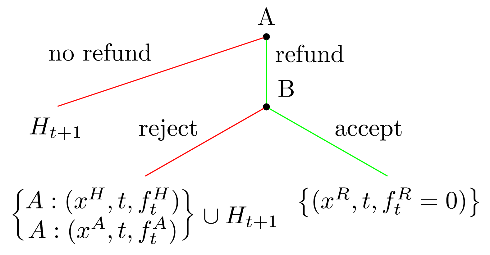
(a) Tree for $H_{t}$ for $t<t^{s}$. If $t=t^{e}$, replace $H_{t+1}$ by $\varnothing$.

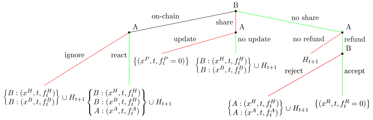
(b) Tree for $H_{t}$ for $t\geq t^{s}$. If $t=t^{e}$, replace $H_{t+1}$ by $\varnothing$.

By the notation $Y\cup H_{t+1}$, we mean that we move on to playing $H_{t+1}$, but that the set $Y$ will be outputted additionally to every leaf of $H_{t+1}$. Whenever a transaction triple is preceded by “$A:$” or “$B:$”, this indicates that Alice or Bob, respectively, will post that transaction triple, and will decide at that point in the game on the transaction fee. In other words, an action is concealed within this node. If this notation is absent, the fee is indicated to be zero, meaning that this transaction will only be included if no other conflicting transactions are posted. This is to simulate the case in which the channel remains open. In that case, no fees are paid and Alice and Bob can keep using the channel. Finally, we have indicated in red the IPB for $t<T$, which amounts to doing nothing as long as the secret is unknown, and Bob sharing it once he learns it, and in green the IPB for $t\geq T$, which amounts to reverting the payment off-chain once the timelock expired.

First of all, note that setting $\mathcal{P}=\overline{\mathbb{N}}_{0}\times\mathbb{N}_{0}$ defines an obvious parametrised application game $(\mathcal{H}^{p})_{p\in\mathcal{P}}$. Second, realise that $\mathcal{H}^{p}$ is essentially a game tree with at each leaf a set of transaction triples. By playing the completed HTLC application game, implied by some $\beta$ and $\omega$, we can replace these sets of transaction triples by utilities for Alice and Bob. Standard computational tools could be used to solve this game, especially for larger $t^{e}$.

We can however make some general statements for the completed HTLC application game. Let us consider the game $\mathcal{H}^{p}$ with $p=(0,T)$, where $T>0$ is the timelock. This specific choice of parameters already captures a lot of interesting behaviour, and is quite general. Indeed, one can convince themselves that at time $t=T$, every strategy that brings the game to the next round $H_{T+1}$ is strictly dominated by an action in $H_{T}$, in which Alice will definitely try to revert the payment or get $x^{A}$ included. Furthermore, we can think of a game with $t^{s}=t^{\prime}>0$ and timelock $T>t^{\prime}$ as a game with $t^{s}=0$ and timelock $T^{\prime}=T-t^{\prime}$.

One can show that for $\mathcal{H}^{(0,T)}$, the IPB as defined in Definition 4.2 is actually not IC w.r.t $\beta_{0}$, where $\beta_{0}$ is modelled by COMG with hashrate distribution $\boldsymbol{\lambda}$. To make it IC, we would have to alter the red lines starting from $t=t^{*}_{m}(\overline{f^{B}},v;\boldsymbol{\lambda},T)$, where $t^{*}_{m}$ is as defined in Theorem 4.1, and where $\overline{f^{B}}$ is the maximum fee Bob is willing to pay for $x^{B}$. Indeed, from that point onward, Alice can force Bob to close the channel and with nonzero probability she will manage to censor Bob’s $x^{B}$, at least forcing Bob to pay a fee higher than $\overline{f^{B}}$ in order to get his $x^{B}$ in (and paying no fees herself), or at best censoring $x^{B}$ and turning a profit herself. This deviation from Alice has a strictly greater expected utility. We will omit the exact description of this IC strategy profile.

On the other hand, notice that for any value of $\overline{f^{B}}$, Bob can choose the timelock $T>0$ accordingly in order for $t^{*}_{m}(\overline{f^{B}},v;\boldsymbol{\lambda},T)$ to be strictly greater than zero. In that case, we will always end up down the path $(\text{share,update})$ in the tree for $H_{0}$, at the end of which Alice and Bob update their channel, as it is not rational for either of them to deviate. Hence, for suitable $T$ and $\overline{f^{B}}$, the IPB will lead to the game ending up down the path $(\text{share,update})$ in the tree for $H_{0}$.

For $T=0$, the IPB indicated in Definition 4.2 is not IC w.r.t. $\beta_{0}$, as Bob is indifferent between updating the channel collaboratively and closing the channel and paying at most $v$ in fees to get $x^{B}$ included (which happens with probability $1/2$) if Alice also pays $v$ in fees to get $x^{A}$ included. Finally, for $t^{s}>T$, the analysis is trivial as Bob will not learn the secret before the game ends. The indicated IPB is again not IC here as in the round $t=T$, Bob is actually indifferent between accepting and rejecting.

4.2.2. Two HTLCs, Two Payment Channels

The HTLC within a PC is arguably among the simplest protocols in the blockchain setting. As we have seen, even this basic construction can fail to be IC. Nonetheless, under certain conditions, Alice and Bob may still adhere—at least partially—to the IPB. We now extend our analysis to a setting with two PCs, each containing an HTLC. While incentive compatibility under $\mathbf{g}$-composition is clearly unattainable, this example offers insight into how compositional effects can reshape incentive structures.

To this end, consider two PCs: one between Alice and Bob, and one between Charlie and Dave. We assume both channels set up their HTLCs at $t=0$, with timelocks $T_{1},T_{2}$, secrets $s_{1},s_{2}$, and values $(v_{A},v_{B},v_{1}),(v_{C},v_{D},v_{2})$, respectively. We model both PCs via parametrised HTLC application games $(\mathcal{H}_{1}^{(t^{s}_{1},t^{e}_{1})})_{(t_{1}^{s},t_{1}^{e})\in\mathcal{P}}$ and $(\mathcal{H}_{2}^{(t^{s}_{2},t^{e}_{2})})_{(t_{2}^{s},t_{2}^{e})\in\mathcal{Q}}$ with $\mathcal{P}=\mathcal{Q}=\overline{\mathbb{N}}_{0}\times\mathbb{N}_{0}$. By defining suitable compositions, we can reason about non-trivial cases where one channel’s behaviour may influence the other. Assume for simplicity that $t_{1}^{e}=t_{2}^{e}=T:=T_{1}\vee T_{2}$. As in the single-channel case, this only removes dominated strategies.

Let us now study, without loss of generality, two kinds of compositions of $(\mathcal{H}^{(p,T)}_{1})_{p\in\overline{\mathbb{N}}_{0}}$ and $(\mathcal{H}^{(q,T)}_{2})_{q\in\overline{\mathbb{N}}_{0}}$. Trivially, we could define the collection $\mathbf{g}^{ind}=(g_{q}^{ind})_{q\in\overline{\mathbb{N}}_{0}}$ where for all $q\in\overline{\mathbb{N}}_{0}$, $g_{q}^{ind}(\sigma_{a,2})=q$ for every $\sigma_{a,2}\in\Sigma_{a,2}^{(q,T)}$. This “independent” composition would correspond with the two channels having nothing to do with each other, except that Bob and Dave learn $s_{1}$ and $s_{2}$, respectively, at the same time $q\in\overline{\mathbb{N}}_{0}$. It is useful to keep in mind that we could have defined the “HTLC in PC”-IPB differently, and would now have been able to apply Theorem 3.12 to conclude that these modified protocols are secure under $\mathbf{g}^{ind}$-composition.

Another collection we could define is $\mathbf{g}^{dep}=(g_{q}^{dep})_{q\in\overline{\mathbb{N}}_{0}}$ where for all $q\in\overline{\mathbb{N}}_{0}$, $g_{q}^{dep}(\sigma_{a,2})=\tau_{C}(\sigma_{a,2})$ for every $\sigma_{a,2}\in\Sigma_{a,2}^{(q,T)}$, where $\tau_{C}(\sigma_{a,2})\in\overline{\mathbb{N}}_{0}$ is the time at which Charlie learns the secret when strategy profile $\sigma_{a,2}\in\Sigma_{a,2}^{(q,T)}$ is chosen. This “dependent” composition essentially reflects a setting in which Charlie and Bob are the same entity (or where Charlie passes the secret on to Bob as soon as he learns it). Note that we could have either $s_{1}=s_{2}$ or $s_{1}\neq s_{2}$; after all, it does not really matter as the composition encapsulates the dynamic that Bob can figure out $s_{1}$ as soon as Charlie learns $s_{2}$.

This dependent composition poses some additional conditions that the two protocols should have had to satisfy in order to be secure under $\mathbf{g}^{dep}$-composition. In particular, consider a CR in which Alice and Dave are one party, and Bob and Charlie are one party. That is, we have the channels Dave-Charlie ($\mathcal{H}_{1}$) and Charlie-Dave ($\mathcal{H}_{2}$). Then $T_{1}$ should be sufficiently larger than $T_{2}$ to prevent Dave from deviating and hence avoiding Charlie losing funds.

Theorem 4.3 (B.3).

In the above setting, with the usual COMG, it is necessary in order for Dave not to deviate from the IPB, that $t^{*}_{m}(\overline{f^{C}_{1}},v_{1};\boldsymbol{\lambda},T_{1})+1\geq t^{*}_{m}(\overline{f^{D}_{2}},v_{2};\boldsymbol{\lambda},T_{2})$.

4.2.3. Wormhole Attack

We conclude this section by noting that the parametrised game approach easily scales to multiple compositions. We could model for example the composition of three channels Alice-Bob, Bob-Charlie and Charlie-Dave. All channels have set up an HTLC at $t=0$, with timelocks $T_{1},T_{2},T_{3}$, secrets $s_{1},s_{2},s_{3}$ and values $(v^{A}_{1},v^{B}_{1},v_{1})$, $(v^{B}_{2},v^{C}_{2},v_{2})$, $(v^{C}_{3},v^{D}_{3},v_{3})$, respectively. We assume moreover that the timelocks satisfy the condition in Theorem 4.3, mutatis mutandis.

The PCs are modelled via parametrised HTLC application games $(\mathcal{H}_{1}^{(t_{1}^{s},T)})_{t_{1}^{s}\in\overline{\mathbb{N}}_{0}}$, $(\mathcal{H}_{2}^{(t_{2}^{s},T)})_{t_{2}^{s}\in\overline{\mathbb{N}}_{0}}$ and $(\mathcal{H}_{3}^{(t_{3}^{s},T)})_{t_{3}^{s}\in\overline{\mathbb{N}}_{0}}$, where we let $T:=T_{1}\vee T_{2}\vee T_{3}$. By clever use of compositions, we can accommodate for the possibility of Bob and Dave colluding, in such a way that Bob learns the secret $s_{1}$ at the same time that Dave learns $s_{3}$. Indeed, we can study the following composition $\mathcal{H}:=\mathcal{H}_{1}\circ_{\mathbf{g}^{12}}\mathcal{H}_{2}\circ_{\mathbf{g}^{23}}\mathcal{H}_{3}$, where $\mathbf{g}^{23}$ would be like $\mathbf{g}^{dep}$, i.e. $\mathbf{g}^{23}=(g_{r}^{23})_{r\in\overline{\mathbb{N}}_{0}}$ with for all $r\in\overline{\mathbb{N}}_{0}$, $g^{23}_{r}(\sigma_{a,3})=\tau_{D}(\sigma_{a,3})$ for every $\sigma_{a,3}\in\Sigma_{a,3}^{r,T}$, and where $\mathbf{g}^{12}$ would be like $\mathbf{g}^{ind}$, i.e. $\mathbf{g}^{12}=(g^{12}_{q})_{q\in\overline{\mathbb{N}}_{0}}$ with for all $q\in\overline{\mathbb{N}}_{0}$, $g^{12}_{q}(\sigma_{a,2})=q$ for every $\sigma_{a,2}\in\Sigma_{a,2}^{q,T}$. From now on, we refer with Dave to both Bob and Dave.

Theorem 4.4 (B.4).

In the above setting, with usual COMG, Dave deviates from the IPB in $\mathcal{H}_{1}\circ_{\mathbf{g}^{12}}\mathcal{H}_{2}\circ_{\mathbf{g}^{23}}\mathcal{H}_{3}$ if $v_{2}>v_{3}$.

In essence, Theorem 4.4 states that Dave will manage to steal the routing fee meant for Charlie, as usually $v_{2}=v_{3}+f_{route}^{C}$ in order to reward $f_{route}^{C}$ Charlie for routing the payment. Charlie, in the meantime, is simply under the impression that the payment failed. This shows that the currently used HTLC construction in for example the Lightning Network is vulnerable to the so-called wormhole attack (Malavolta et al., 2018). Mitigations to this attack are known, which in terms of our framework would make it impossible to have the $\mathbf{g}^{12}$-composition as we defined it now, forcing a dependent composition of $\mathcal{H}_{1}$ and $\mathcal{H}_{2}$, similar to $\mathbf{g}^{23}$.

4.2.4. A CRAB Payment Channel

Unlike the prior examples, where the structure of the underlying PC was kept implicit, we now consider a specific construction in detail. In particular, Lightning-style channels are known to be vulnerable to bribing attacks when miners behave rationally (Aumayr et al., 2024). To address this, Aumayr et al. (2024) introduced the CRAB channel, a design that mitigates such attacks. The core idea is to let the participants each put in an additional collateral $c$ into the channel, that will be rewarded to a miner in case a participant misbehaves by publishing an old channel state. The CRAB construction introduces a delay $T$ before which the party closing the channel cannot claim their balance. In Appendix A, we write the CRAB channel closing protocol as an application game $\mathcal{K}^{T}$, which leads us to the following result.

Theorem 4.5 (B.5).

In, $(\mathcal{K}^{T},\mathcal{B}_{0,\mathcal{K}^{T}},\omega)$, Alice will not post an old commitment transaction if $T>\lceil\rho_{m}(c,v;\boldsymbol{\lambda})\rceil$, where $\boldsymbol{\lambda}$ is the hashrate distribution assumed in $\mathcal{B}_{0,\mathcal{K}^{T}}$.

Remark 4.6.

If we assume the worst-case hashrate distribution $\boldsymbol{\lambda}=(0,\frac{1}{2},\frac{1}{2})$, we have $\rho_{1}=\rho_{2}$ equal to $0$ if $\frac{c}{v}>\frac{1}{2}$ and equal to $\infty$ otherwise, so we retrieve the same condition as Aumayr et al. (2024) that $c>\frac{v}{2}$ in order for Alice not to post an old commitment transaction. We stress once again that we can easily keep the application game as is and study the CRAB channel under different blockchain assumptions without changing the proof.

4.3. A Simple Example of MEV

The previous examples focused on how application-layer strategies interact with a fixed blockchain model. We now shift focus to the network layer, exploring how transaction propagation itself can shape incentives and strategic behaviour. Until now, the network game has been kept intentionally simple: all players in the blockchain game receive the full set of transaction triples produced by the application game. We now consider a richer network game where application-layer players can selectively forward transactions to specific blockchain participants. This models limited propagation which can influence MEV outcomes and strategic behaviour.

Consider the following abstract model of a DeFi smart contract where a user $U$ makes a trade by placing a buy limit order, i.e., a transaction $x_{U}$, that buys some asset for a price up to $l$. The current price is $l-s$, with $s\geq 0$, and so if $x_{U}$ were included as is, $U$ would have utility $s$. However, the miners are also able to interact with the smart contract and are thus part of the application game. Upon seeing $x_{U}$, each miner has the capability to front- and backrun, or sandwich, $x_{U}$. In particular, each miner $j\in M$ could add a transaction $x_{F,j}$ before $x_{U}$ buying the asset at price $l-s$, and a transaction $x_{B,j}$ after $x_{U}$, selling the asset again at price $l$. In doing so, the miner captures $s$ and $U$ is left with utility $0$, as the transaction now buys at price $l$ instead of $l-s$.

We model this by playing the application game $\mathcal{A}=(\quantity{U}\cup M,\{x_{U}\}\cup\{x_{F,j},x_{B,j}\}_{j\in M},\Sigma_{a},\pi_{a})$. The set $M$ contains the miners, who are all part of the application game and can thus monitor the intents of other players. The strategy profile set $\Sigma_{a}$ reflects this by corresponding to a simultaneous game in which each miner gets to decide whether or not construct sandwiching transactions, upon seeing $x_{U}$. We will assume that $(x_{U},0,f)\in\pi_{a}(\sigma_{a})$ for each $\sigma_{a}\in\Sigma_{a}$, with $f>0$ some fixed fee. Afterwards, we play for a given $\pi_{a}(\sigma_{a})$ a network game where $U$ gets to decide to which miners to send $(x_{U},0,f)$, i.e., the network game $\mathcal{N}=(\quantity{U},M,\pi_{a}(\sigma_{a}),\mathscr{P}(M),\pi_{ng})$, where $\sigma_{ng}\in\mathscr{P}(M)$ is the strategy profile containing the set of miners that $U$ chose to share $x_{U}$ with, and $\pi_{ng}(\sigma_{ng})$ is the tuple $(\pi_{ng,j}(\sigma_{ng}))_{j\in M}$ where for each $j\in M$, $\pi_{ng,j}(\sigma_{ng})$ is defined as $\pi_{a}(\sigma_{a})\cap\{(x_{F,j},0,0),(x_{B,j},0,0)\}$ if $j\in\sigma_{ng}$ and $\pi_{a}(\sigma_{a})\cap\{(x_{F,j},0,0),(x_{B,j},0,0)\}\setminus\{(x_{U},0,f)\}$ otherwise. Remark that although the miners might already know $U$ wants to make the trade $x_{U}$, they would only be willing to sandwich $x_{U}$ if they have actually received $x_{U}$ as input to the blockchain game.

For a given $\pi_{ng}(\sigma_{ng})$, the subsequent blockchain game is given by $(M,\pi_{ng}(\sigma_{ng}),\Sigma_{bg},\pi_{bg})$. We specify $\Sigma_{bg}=\quantity{H,D}^{\quantity|M|}$, where each miner decides whether to ($H$) just include $x_{U}$, or to ($D$) sandwich $x_{U}$, if they were to receive the transaction $x_{U}$. One miner $j\in M$ then gets selected at random (proportional to its hashrate) to propose the blockchain ordering, which will either be $b=b_{H,j}$ (containing only $x_{U}$) or $b=b_{D,j}$ (containing $x_{F,j},x_{U},x_{B,j}$). This implicitly defines the ordering function $\pi_{bg}$. We moreover specify, for each possible ordering $b$, the execution function $\omega$ for $U$ as $\omega_{U}(b)=s$ if $b=b_{H,j}$ for some $j\in M$ and $\omega_{U}(b)=0$ if $b=b_{D,j}$ for some $j\in M$, and for each $j\in M$ as $\omega_{j}(b)=f\mathbbm{1}_{b=b_{H,j}}+(f+s)\mathbbm{1}_{b=b_{D,j}}$.

From the above formulation, it is clear that without any additional measures, the miners will always choose strategy $D$. Given that, $U$ will always end up with zero utility and does not have any preference with regards to which miner to share $(x_{U},0,f)$ with. A simple countermeasure to this inevitable MEV scenario would be to introduce a trusted miner, holding a proportion $\lambda_{H}$ of the hashrate. We can model this miner as a player with only the strategy $H$ (or equivalently assign a utility of $-\infty$ to any strategy profile where this miner has strategy $D$). Consequently, it is clear that $U$ will only share $(x_{U},0,f)$ with the trusted miner.

4.4. Broader Applications

Our framework is designed to facilitate compositional reasoning in complex blockchain environments where incentive alignment arises from the interaction of multiple protocols and layers. While earlier case studies have formalised specific constructions, the framework naturally generalises to a broader class of real-world settings. This subsection outlines three principal categories that reflect common compositional patterns in practice, each introducing distinct modelling requirements and incentive dynamics. Detailed examples are provided in Appendix C.

1. Cross-application composition: Multiple decentralised applications (dApps) share a common blockchain infrastructure and may interact implicitly through shared state or timing dependencies. Representative examples include arbitrage between decentralised exchanges (DEXs) or oracle-driven feedback loops, where strategic behaviour emerges only from the interplay of otherwise independent systems.

2. Cross-blockchain composition: Protocols such as atomic swaps coordinate actions across independent blockchains with distinct execution environments and trust models. By treating each chain as a separate game and specifying inter-chain dependencies explicitly, our framework enables modular analysis under heterogeneous assumptions.

3. Complex Network and Multi-layer Dynamics: Architectures like proposer-builder separation (PBS) span the application, network, and consensus layers. Our model treats each layer explicitly, supporting rigorous reasoning about how network-level logic (e.g., auctions among builders) and consensus-level inclusion policies jointly affect incentive compatibility.

These categories illustrate how the framework accommodates modern protocol designs that defy traditional single-layer analysis. Concrete examples corresponding to each setting are outlined informally in Appendix C, focusing on how the framework could be instantiated to capture the relevant dynamics. Although these use cases are not fully formalised, they demonstrate how modular reasoning can be leveraged to isolate critical assumptions, detect edge-case vulnerabilities, and explore design alternatives.

Crucially, each category supports meaningful questions that would be difficult to approach without a layered and compositional model. In cross-application scenarios, it enables formal reasoning about whether composability introduces profitable but unintended deviations, e.g., does arbitrage across DEXs destabilise pricing mechanisms, or can oracle design be hardened against feedback-driven manipulation? In cross-chain protocols, our framework provides the structure to analyse swap soundness under heterogeneous security assumptions, e.g., how do differences in block times, censorship resistance, or finality affect incentive compatibility? Finally, in multi-layer systems such as PBS and MEV auctions, the framework enables principled mechanism design: which auction formats discourage censorship? When does exclusive order flow lead to centralisation? How should fees and rebates be structured to align incentives across builders, searchers, and proposers? These examples demonstrate how the layered, compositional design of our framework provides a modular and rigorous foundation for evaluating incentive properties in emerging blockchain protocols.

5. Conclusion

In this work, we presented a compositional framework for analysing the game-theoretic security of blockchain protocols. Unlike traditional approaches that analyse individual protocols in isolation or assume fixed-layer behaviour, our model embraces the modular structure of modern blockchain ecosystems by decomposing them into layered games. Each layer—the application, network, and blockchain—is formalised as a strategic game, and interactions are expressed through explicitly defined interfaces. This layered architecture allows us to reason not only about the behaviour of each component but also about how incentive flows propagate across the system.

At the core of our approach lies the definition of cross-layer games and cross-application composition, which enable reasoning about concurrent protocol execution and emerging vulnerabilities such as bribing, censorship, and MEV. These abstractions support modular security analysis: properties of individual layers or protocols can be verified and then composed, facilitating the study of more complex interactions without rederiving the entire system’s behaviour. Our use of parametrised games further introduces modelling flexibility, allowing protocols to interleave in time or through shared components.

Through detailed case studies, we demonstrate the expressiveness and utility of our framework. These examples show how existing incentive misalignments can be captured and formalised, revealing both subtle vulnerabilities and new levers for robust protocol design.

This work also opens several directions for future research. First, extending the framework to capture richer network models, including asynchronous message propagation, selective delivery, or targeted censorship, would better reflect the operational characteristics of blockchain networks. Second, formalising the translation from protocol specifications to application games is essential to enable broader applicability and automation. Third, identifying the classes of protocols that satisfy compositional incentive compatibility under various assumptions would clarify the expressive limits of the framework. Finally, generalising the framework to support parametrised families of blockchain environments, e.g., based on hashrate distributions or latency assumptions, and exploring alternative definitions of incentive compatibility could yield practically relevant, robust security guarantees across diverse deployments.

Our framework bridges a long-standing gap between incentive-aware protocol analysis and modular security reasoning. It provides a foundation for understanding the strategic behaviour of blockchain participants in complex, multi-protocol environments and contributes to the development of provably secure, incentive-aligned decentralised systems.

Appendix A CRAB Payment Channels in Detail

The CRAB construction is illustrated in Figure 2.

Figure 2. Transaction flow for a CRAB PC

Just as in standard Lightning channels, the CRAB channel locks its capacity in a 2-of-2 multisignature output via a transaction $x_{F}$. Each participant can unilaterally broadcast a commitment transaction that closes the channel and distributes the funds on-chain. In Figure 2, we specified Alice’s $k$-th commitment transaction $x_{A,C}^{k}$. These commitment transactions are regularly updated to reflect the latest balances, but earlier (outdated) versions remain valid and can still be broadcast. To discourage this, participants exchange revocation keys during updates, enabling the other party to claim the entire channel balance through a punishment transaction if an old commitment is posted. For example, when updating from state $k$ to state $k+1$, Alice will share $r_{A}^{k}$ with Bob and Bob will give $r_{B}^{k}$ to Alice. Because there is a timelock $T$, Alice cannot immediately post $x_{A,S}^{k}$ to claim her funds, giving Bob the opportunity to punish her by posting $x_{A,P}^{k}$ in case state $k$ would be an old state. The second output $c$ in $x_{A,P}^{k}$ can be claimed by anyone, and will thus be claimed by the miner who includes $x_{A,P}^{k}$.

In standard Lightning, rational miners may be bribed to include an outdated commitment transaction while censoring the corresponding punishment transaction—resulting in fund loss for the honest party. CRAB channels mitigate this by requiring both participants to lock up collateral, which is forfeited to the miner if a party attempts to close the channel dishonestly using an old commitment. Using our framework, we analyse under which conditions such misbehaviour becomes unprofitable with respect to the COMG.

Consider a CRAB channel between Alice and Bob. Alice wishes to close the channel and can choose to broadcast either her most recent commitment transaction $x_{A,C}^{l}$, reflecting balances $v_{A}^{l}$ and $v_{B}^{l}$, or an outdated one $x_{A,C}^{o}$, reflecting $v_{A}^{o}$ and $v_{B}^{o}$. She may also choose whether to attach a corresponding spending transaction $x_{A,S}^{l}$ or $x_{A,S}^{o}$. If Alice posts $x_{A,C}^{o}$, Bob can retaliate by broadcasting a punishment transaction $x_{A,P}^{o}$, which gives him Alice’s balance and the miner her collateral. Alice can try to prevent this by raising the fee on $x_{A,S}^{o}$, effectively bribing miners to ignore the punishment. Bob may counter-bribe by increasing the fee on his punishment transaction. This fee race continues until the timelock expires, allowing Alice to settle using $x_{A,S}^{o}$ if the punishment was successfully censored.

We model this interaction as an application game $\mathcal{K}$ with player set $N=\quantity{A,B}$, and $(X,\Sigma_{a},\pi_{a})$ defined via a recursive extensive-form game. The game unfolds as a sequence $(K_{t})_{t=-1}^{T}$, illustrated in Figures 3 and 4.

Figure 3. Tree for $K_{-1}$.

Figure 4. Tree for $K_{t}$ for $0\leq t\leq T$. If $t=T$, replace $K_{t+1}$ by $\varnothing$.

We can prove a sufficient condition for Alice not posting old commitment transactions in the parametrised cross-layer game $(\mathcal{K}^{T},\mathcal{B}_{0,\mathcal{K}^{T}},\omega)$. Here, $\omega$ can be defined via $\tilde{\omega}$ as in Definition 3.1 by:

$$\tilde{\omega}_{A}(b) =\begin{cases}v_{A}^{l}+c,&b\supseteq\{x_{A,C}^{l},x_{A,S}^{l}\},\\ v_{A}^{o}+c,&b\supseteq\{x_{A,C}^{o},x_{A,S}^{o}\},\\ 0,&b\supseteq\{x_{A,C}^{o},x_{A,P}^{o}\},\end{cases}$$

$$\tilde{\omega}_{B}(b) =\begin{cases}v_{B}^{l}+c,&b\supseteq\{x_{A,C}^{l}\},\\ v_{B}^{o}+c,&b\supseteq\{x_{A,C}^{o}\},\\ v+c,&b\supseteq\{x_{A,C}^{o},x_{A,P}^{o}\},\end{cases}$$

$$\tilde{\omega}_{j}(b) =\begin{cases}c,&b\supseteq\{x_{A,C}^{o},x_{A,P}^{o}\}\\ 0,&\text{otherwise},\end{cases}$$

where $j$ is the miner who included $x_{A,P}^{o}$. With the notation $b\supseteq S$ we mean every blockchain ordering that prioritises the transactions in $S$ over any possible transactions that might spend the same funds as the transactions in $S$, by either putting the former transactions earlier in the ordering than the latter, or not including the latter in the ordering at all.

Appendix B Proofs

B.1. Proof of Theorem 3.12

For ease of notation, we will for this proof write $\sigma$ and $\Sigma$ instead of $\sigma_{a}$ and $\Sigma_{a}$ for strategies and strategy profiles in the application game. Let us first define the concept of a projection on a player subset, which will be useful in a bit.

Definition B.1 (Projection on a player subset).

For a player set $N$, and a subset $S\subseteq N$, we say that the transformation $\eta_{S}:S\to S$ is a projection on S of the transformation $\eta:N\to N$, if for every $i\in S$ we have

$$\eta_{S}(i)=\begin{cases}\eta(i),&\eta(i)\in S,\\ \zeta(\eta(i)),&\eta(i)\notin S,\end{cases}$$

for some injective map $\zeta:\eta(S)\setminus S\rightarrow S\setminus\eta(S)$, defined whenever $\eta(S)\setminus S\neq\varnothing$.

It suffices to show that for each value of the parameter $p\in\mathcal{P}$, $(((\mathcal{A}_{2}\circ_{\mathbf{g}}\mathcal{A}_{1})^{p},\beta,\omega),\overline{\sigma}^{p})$ is IC w.r.t $\beta$ (implying player set $M$), where $\mathbf{g}$ is a collection $(g_{p})_{p\in\mathcal{P}}$ of constant functions. We proceed by contradiction. Fix some $p\in\mathcal{P}$, let $\eta:N\cup M\to N\cup M$ (with $N=N_{1}\cup N_{2}$) be some transformation, and denote by $\tilde{\mathcal{A}}$ the $\eta$-CR of $\mathcal{A}:=(\mathcal{A}_{2}\circ_{\mathbf{g}}\mathcal{A}_{1})^{p}$. We will derive a contradiction by assuming that the strategy profile $\overline{\sigma}^{p}:=(\overline{\sigma}_{1}^{p},(\overline{\sigma}_{2}^{g_{p}(\sigma_{1})})_{\sigma_{1}\in\Sigma_{1}^{p}})$, which we will refer to as $\overline{\sigma}=(\overline{\sigma}_{1},\overline{\sigma}_{2})$ as $p\in\mathcal{P}$ is fixed and $g_{p}(\overline{\sigma}_{1})=q_{p}$ for some constant $q_{p}\in\mathcal{Q}$, is not a Nash equilibrium for $(\tilde{\mathcal{A}},\beta,\omega)$. That is, in $(\tilde{\mathcal{A}},\beta,\omega)$ there exists a deviation $\sigma=(\sigma_{1},\sigma_{2})$ by some player $k\in N\cup M$ such that $u_{k}(\sigma)>u_{k}(\overline{\sigma})$.

Let us denote by $\eta_{1}$ and $\eta_{2}$ the projections of $\eta$ on $N_{1}\cup M$ and $N_{2}\cup M$, as defined in Definition B.1. These projections define CRs $\tilde{\mathcal{A}}_{1}$ of $\mathcal{A}_{1}$ and $\tilde{\mathcal{A}}_{2}$ of $\mathcal{A}_{2}$, respectively. It should be clear by additivity of the execution function, and by the fact that the utility of a collusion of players is the sum of the utilities of the individual players in that collusion, that $u_{k}(\sigma)=u_{1,k_{1}}(\sigma_{1})+u_{2,k_{2}}(\sigma_{2})$, and $u_{k}(\overline{\sigma})=u_{1,k_{1}}(\overline{\sigma}_{1})+u_{2,k_{2}}(\overline{\sigma}_{2})$, where $k_{1}=\eta_{1}(\eta^{-1}(k)\cap(N_{1}\cup M))$ and $k_{2}=\eta_{2}(\eta^{-1}(k)\cap(N_{2}\cup M))$. But then, by assumption,

$$u_{1,k_{1}}(\sigma_{1})+u_{2,k_{2}}(\sigma_{2})>u_{1,k_{1}}(\overline{\sigma}_{1})+u_{2,k_{2}}(\overline{\sigma}_{2}),$$

which means that $u_{1,k_{1}}(\sigma_{1})>u_{1,k_{1}}(\overline{\sigma}_{1})$ or $u_{2,k_{2}}(\sigma_{2})>u_{2,k_{2}}(\overline{\sigma}_{2})$. But then, $\sigma_{1}$ is a profitable deviation by $k_{1}$ from $\overline{\sigma}_{1}$ in $(\tilde{\mathcal{A}}_{1},\beta,\omega)$, or $\sigma_{2}$ is a profitable deviation by $k_{2}$ from $\overline{\sigma}_{2}$ in $(\tilde{\mathcal{A}}_{2},\beta,\omega)$. This contradicts $\Pi_{1}$ and $\Pi_{2}$ being both IC w.r.t. $\beta$.

B.2. Proof of Theorem 4.1

For ease of notation, we will for this proof write $\sigma$ instead of $\sigma_{bg}$ for strategies and strategy profiles in the COMG. We will work our way backwards, starting at round $T$. For each round $t=0,\ldots,T$, and for each miner $j=1,\ldots,m$, we will compute the expected gain $v_{j}^{t}\quantity(\sigma_{j}^{t};(\sigma_{j}^{s})_{s=t+1}^{T})$, where $\sigma_{j}^{s}\in\quantity{1,2}$ denotes the decision taken by miner $j$ at time $s$, where $\sigma_{j}^{s}=1$ encodes the miner trying to include $x_{1}$ in round $s$, and $\sigma_{j}^{s}=2$ encodes the miner censoring $x_{1}$ in round $s$, or including $x_{2}$ if possible.

For miner $j=1,\ldots,m$ we have the following expected gain in round $T$:

(2) $$v_{j}^{T}\quantity(\sigma_{j}^{T})=\begin{cases}\lambda_{j}f_{1},&\sigma_{j}^{T}=1,\\ \lambda_{j}f_{2},&\sigma_{j}^{T}=2.\end{cases}$$

By assumption, $f_{1}<f_{2}$ and so in round $T$ all miners will include $x_{2}$. Keep in mind that in the COMG, we also consider a portion of the hashrate $\lambda_{0}$ that will by construction always include $x_{1}$ in rounds before $T$, and will switch to including $x_{2}$ only in round $T$ as it is the more rewarding transaction to include.

For rounds $t<T$, the expected gain depends on what players expect to gain in subsequent rounds. For example, at a round $t<T$, a miner $j$ can decide whether to include $x_{1}$. Out of the remaining miners, there will be a portion of hashrate $\lambda_{I,j}^{t}$ that will include $x_{1}$ at round $t$, and a portion of hashrate $\lambda_{C,j}^{t}$ that will censor $x_{1}$ at round $t$. Hence, with probability $\lambda_{I,j}^{t}$, in round $t$ another miner will mine a block including $x_{1}$, leaving $j$ with a zero gain. With probability $\lambda_{C,j}^{t}$, another miner will mine a block in round $t$ excluding $x_{1}$, leading to miner $j$ having to decide in round $t+1$ again whether or not to include $x_{1}$. If we assume that $j$’s decision in round $t+1$ leads to an expected gain of $g$, $j$ will have with probability $\lambda_{C,j}^{t}$ a gain of $g$. This reasoning leads us to the following recursive expression for the expected gain in round $t=0,\ldots,T-1$:

$$v_{j}^{t}\quantity(\sigma_{j}^{t};(\sigma_{j}^{s})_{s=t+1}^{T})=$$

(3) $$\begin{cases}\lambda_{j}f_{1}+\lambda_{C,j}^{t}v_{j}^{t+1}\quantity(\sigma_{j}^{t+1};(\sigma_{j}^{s})_{s=t+2}^{T}),&\sigma_{j}^{t}=1,\\ \lambda_{j}v_{j}^{t+1}\quantity(\sigma_{j}^{t+1};(\sigma_{j}^{s})_{s=t+2}^{T})+\lambda_{C,j}^{t}v_{j}^{t+1}\quantity(\sigma_{j}^{t+1};(\sigma_{j}^{s})_{s=t+2}^{T}),&\sigma_{j}^{t}=2.\end{cases}$$

Hence, if $f_{1}<v_{j}^{t+1}\quantity(\sigma_{j}^{t+1};(\sigma_{j}^{s})_{s=t+2}^{T})$, $j$ will choose to censor $x_{1}$ instead of including it.

For each miner $j=1,\ldots,m$, we are interested in the strategy $(\sigma_{j}^{s})_{s=0}^{T}$ that maximises the expected gain $v_{j}^{0}$. First of all, we claim that this optimal strategy is always of the the form $(1,\ldots,1,2,\ldots,2)$. That is, a miner will always include $x_{1}$ up to some point, after which this miner switches to censoring $x_{1}$, never trying to include it again.

Lemma B.2.

For a fixed miner $j=1,\ldots,m$, the strategy $(\overline{\sigma}_{j}^{t})_{t=0}^{T}$ that maximises the expected gain $v_{j}^{0}$ is of the form

(4) $$\overline{\sigma}_{j}^{t}=\begin{cases}1,&t<t_{j}^{*},\\ 2,&t\geq t_{j}^{*}.\end{cases}$$

for some $t_{j}^{*}\in\quantity{0,\ldots,T}$.

Proof.

Clearly, since $f_{1}<f_{2}$, $\overline{\sigma}_{j}^{T}=2$. Let us now assume that for some $t\in\quantity{1,\ldots,T}$, and given a sequence $(\overline{\sigma}_{j}^{s})_{s=t+1}^{T}$, we have $\overline{\sigma}_{j}^{t}=1$. By Equation (B.2), this implies that $f_{1}\geq v_{j}^{t+1}\quantity((\overline{\sigma}_{j}^{s})_{s=t+1}^{T})$. Again by Equation (B.2), we find that

$$v_{j}^{t}\quantity(\overline{\sigma}_{j}^{t};(\overline{\sigma}_{j}^{s})_{s=t+1}^{T}) =(\lambda_{j}+\lambda_{C,j}^{t})v_{j}^{t+1}\quantity(\overline{\sigma}_{j}^{t+1};(\overline{\sigma}_{j}^{s})_{s=t+2}^{T})$$

$$\leq(\lambda_{j}+\lambda_{C,j}^{t})f_{1}\leq f_{1}.$$

But then, using Equation (B.2) one last time for round $t-1$, we find $v_{j}^{t-1}\quantity(1;(\overline{\sigma}_{j}^{s})_{s=t}^{T})\geq v_{j}^{t-1}\quantity(2;(\overline{\sigma}_{j}^{s})_{s=t}^{T})$. Hence, $\overline{\sigma}_{j}^{t-1}=1$. By an induction argument, this implies that if we have $\overline{\sigma}_{j}^{t}=1$ at some round $t\in\quantity{0,\ldots,T-1}$, we have $\overline{\sigma}_{j}^{s}=1$ for all $s<t$ as well. By contraposition and a similar induction argument, if we have $\overline{\sigma}_{j}^{t}=2$ at some round $t\in\quantity{0,\ldots,T-1}$, we must also have $\overline{\sigma}_{j}^{s}=2$ for all $s>t$. Consequently, the optimal strategy must be of the form specified in (4). ∎

By Lemma B.2, determining the optimal strategy for each miner amounts to finding the round $t_{j}^{*}$ at which miner $j$ switches from including $x_{1}$ to censoring $x_{1}$, for each $j=1,\ldots,m$. Combining (2), (B.2), and (4), we know that for any miner $j=1,\ldots,m$, the expected gain for $t\geq t_{j}^{*}$ is given by

(5) $$v_{j}^{t}\quantity((\overline{\sigma}_{j}^{s})_{s=t}^{T})=\quantity(\prod_{s=t}^{T-1}\lambda_{C}^{s})\lambda_{j}f_{2},$$

where for $t\geq t_{j}^{*}$, we defined $\lambda_{C}^{t}=\lambda_{j}+\lambda_{C,j}^{t}$ as the total portion of hashrate that is censoring $x_{1}$ in round $t$. Now remark that if we have $\overline{\sigma}_{j}^{t}=2$, we have $v_{j}^{t+1}\quantity((\overline{\sigma}_{j}^{s})_{s=t+1}^{T})>f_{1}$. Consequently, for any miner $k\in\quantity{j+1,\ldots,m}$, which has by Definition 2.6 a hashrate $\lambda_{k}\geq\lambda_{j}$, (5) implies that,

$$v_{k}^{t+1}\quantity((\overline{\sigma}_{k}^{s})_{s=t+1}^{T}) =\quantity(\prod_{s=t+1}^{T-1}\lambda_{C}^{s})\lambda_{k}f_{2}$$

$$\geq\quantity(\prod_{s=t+1}^{T-1}\lambda_{C}^{s})\lambda_{j}f_{2}$$

$$=v_{k}^{t+1}\quantity((\overline{\sigma}_{j}^{s})_{s=t+1}^{T})>f_{1}.$$

where the first equality holds whenever $t+1\geq t_{k}^{*}$. That is, $\overline{\sigma}_{k}^{t}=2$. By induction, one can easily find the following Corollary.

Corollary B.3.

Assume that $\lambda_{j}\leq\lambda_{k}$ for some $j,k\in\quantity{1,\ldots,m}$. Then $\overline{\sigma}_{j}^{t}=2$ implies that $\overline{\sigma}_{k}^{t}=2$.

In other words, larger miners will start censoring $x_{1}$ before smaller miners.

Starting at $t=T$ and working our way backwards, we will have an ever-shrinking set of censoring miners, where going further back in time will result in the smallest miner that is still censoring switching to including $x_{1}$. To compute the times $t_{j}^{*}$ for all $j=1,\ldots,m$, it will therefore be easier to sometimes work with the reverse time $r:=T-t$, looking backwards starting from $t=T$ and computing the value $r^{*}_{j}:=T-t_{j}^{*}$, starting from the smallest miner and working our way up.

At $r=0$ (that is, $t=T$), we have already established that all miners will go for $x_{2}$. At $r=1$, (B.2) tells us that miner $j\in\quantity{1,\ldots,m}$ will censor $x_{1}$ as long as $f_{1}<\lambda_{j}f_{2}$. In other words, all miners with a hashrate smaller than or equal to $f_{1}/f_{2}$ will include $x_{1}$ at $r=0$ (which is round $T-1$). Say there are $\ell$ miners with such a small hashrate, i.e., $\lambda_{1}\leq\ldots\lambda_{\ell}\leq f_{1}/f_{2}<\lambda_{\ell+1}$. Then for all $j=1,\ldots,\ell$, we have $r_{j}^{*}=0$ and so $t_{j}^{*}=T$.

Let us now consider miner $j=\ell+1$. This miner will still censor at $r=1$, but how long will this miner keep censoring? We are looking for the smallest value of $t$ for which $v_{\ell+1}^{t+1}\quantity((2)_{s=t+1}^{T})>f_{1}$. In other words, by Equation 5, we are looking for the smallest $t$ for which

$$\quantity(\prod_{s=t+1}^{T-1}\lambda_{C}^{s})\lambda_{\ell+1}f_{2}>f_{1}.$$

We know that the hashrate $\sum_{k=1}^{\ell}\lambda_{k}$ is already trying to include $x_{1}$, and that for all rounds larger than this smallest $t$, $j=\ell+1$ will be censoring. Hence, by Corollary B.3, we know that the portion $\sum_{k=\ell+1}^{m}\lambda_{k}$ of hashrate will censor $x_{1}$. That is, $\lambda_{C}^{s}=\sum_{k=\ell+1}^{m}\lambda_{k}=1-\lambda_{0}-\sum_{k=1}^{\ell}\lambda_{k}$ for $s=t,\ldots,T-1$. We are thus looking for $r_{\ell+1}^{*}$, the largest $r$ such that

$$\quantity(\sum_{k=\ell+1}^{m}\lambda_{k})^{r-1}\lambda_{\ell+1}f_{2}>f_{1}.$$

It is easy to see that since $r\in\mathbb{N}_{0}$, $r_{\ell+1}^{*}-1=\lfloor\rho_{\ell+1}\rfloor$, where $\rho_{\ell+1}$ satisfies

$$\quantity(\sum_{k=\ell+1}^{m}\lambda_{k})^{\rho_{\ell+1}}\lambda_{\ell+1}f_{2}=f_{1}\implies\rho_{\ell+1}=\frac{\log\frac{f_{1}}{\lambda_{\ell+1}f_{2}}}{\log\sum_{k=\ell+1}^{m}\lambda_{k}}.$$

In other words, we have $r_{\ell+1}^{*}=\lceil\rho_{\ell+1}\rceil$. Moving on, for the next miner $j=\ell+2$, we know that $r_{j}^{*}\geq r_{\ell+1}^{*}$. For $r>r_{\ell+1}^{*}$, miner $\ell+1$ is no longer censoring $x_{1}$, hence from then on we have a portion $\sum_{k=\ell+2}^{m}\lambda_{k}$ censoring $x_{1}$. We are thus looking for the largest $r$ such that

$$\quantity(\sum_{k=\ell+2}^{m}\lambda_{k})^{r-r_{\ell+1}^{*}-1}\quantity(\sum_{k=\ell+1}^{m}\lambda_{k})^{r_{\ell+1}^{*}}\lambda_{\ell+2}f_{2}>f_{1}.$$

Again, since $r\in\mathbb{N}_{0}$, we have $r_{\ell+2}^{*}-1=\lfloor\rho_{\ell+2}\rfloor$, and so $r_{\ell+2}^{*}=\lceil\rho_{\ell+2}\rceil$, where $\rho_{\ell+2}$ is defined by

$$\quantity(\sum_{k=\ell+2}^{m}\lambda_{k})^{\rho_{\ell+2}-\lceil\rho_{\ell+1}\rceil}\quantity(\sum_{k=\ell+1}^{m}\lambda_{k})^{\lceil\rho_{\ell+1}\rceil}\lambda_{\ell+2}f_{2}=f_{1},$$

which implies

$$\rho_{\ell+2}=\lceil\rho_{\ell+1}\rceil+\frac{\log\frac{f_{1}}{\lambda_{\ell+2}f_{2}}-\lceil\rho_{\ell+1}\rceil\log\quantity(\sum_{k=\ell+1}^{m}\lambda_{k})}{\log\sum_{k=\ell+2}^{m}\lambda_{k}}.$$

Repeating this argument inductively, one can see that more generally, for miner $j\in\quantity{\ell+1,\ldots,m}$, we have $r_{j}^{*}=\lceil\rho_{j}\rceil$, where $\rho_{j}$ satisfies

$$\quantity(\sum_{k=j}^{m}\lambda_{k})^{\rho_{j}-\lceil\rho_{j-1}\rceil}\prod_{i=\ell+1}^{j-1}\quantity(\quantity(\sum_{k=i}^{m}\lambda_{k})^{\lceil\rho_{i}\rceil-\lceil\rho_{i-1}\rceil})\lambda_{j}f_{2}=f_{1}.$$

where we set $\rho_{\ell}=0$. This gives us the following recursion for $\rho_{j}$:

(6) $$\rho_{j}=\lceil\rho_{j-1}\rceil+\frac{\log\frac{f_{1}}{\lambda_{j}f_{2}}-\sum_{i=\ell+1}^{j-1}\quantity(\lceil\rho_{i}\rceil-\lceil\rho_{i-1}\rceil)\log\quantity(\sum_{k=i}^{m}\lambda_{k})}{\log\sum_{k=j}^{m}\lambda_{k}}.$$

This identity allows us to compute recursively the values $r_{j}^{*}=\lceil\rho_{j}\rceil$ for every $j\in\quantity{\ell+1,\ldots,m}$, for any given hashrate distribution $\boldsymbol{\lambda}$ and fees $f_{1},f_{2}$.

Now, given the values $(r_{j}^{*})_{j=1}^{m}$ (keep in mind that $r_{j}^{*}=0$ for $j=1,\ldots,\ell$), we can write down the probability $p(T;\boldsymbol{\lambda},f_{1},f_{2})$ that $x_{1}$ will be included instead of $x_{2}$, as a function of the timelock $T$. Clearly, if $T>r_{m}^{*}$, there will be at least one round in which all the miners will try to mine a block that includes $x_{1}$, so $x_{1}$ will be included with probability $1$. Trivially, since $f_{2}>f_{1}$, if $T=0$, all miners will go for $x_{2}$ and so $x_{1}$ will be included with probability $0$. Now, suppose that $T>r_{j-1}^{*}$ and $T\leq r_{j}^{*}$ for some $j\in\quantity{1,\ldots,m}$ (we set $r_{0}^{*}=0$). Then the probability that $x_{1}$ is censored for $T$ rounds is $\prod_{s=0}^{T-1}\lambda_{C}^{s}$. Since $\lambda_{C}^{s}=\sum_{k=j}^{m}\lambda_{k}$ for $s=r_{j-1}^{*}+1,\ldots,r_{j}^{*}$, we can write

(7) $$p(T;\boldsymbol{\lambda},f_{1},f_{2})=1-\quantity(\sum_{k=j}^{m}\lambda_{k})^{T-r_{j-1}^{*}}\prod_{i=1}^{j-1}\quantity(\quantity(\sum_{k=i}^{m}\lambda_{k})^{r_{i}^{*}-r_{i-1}^{*}}).$$

B.3. Proof of Theorem 4.3

Suppose that $t^{*}_{m}(\overline{f^{C}_{1}},v_{1};\boldsymbol{\lambda},T_{1})+1<t^{*}_{m}(\overline{f^{D}_{2}},v_{2};\boldsymbol{\lambda},T_{2})$. Dave will deviate from the intended protocol behaviour in $\mathcal{H}_{2}$ by not sharing the secret with Charlie until $\tilde{t}:=t^{*}_{m}(\overline{f^{C}_{1}},v_{1};\boldsymbol{\lambda},T_{1})+1$. At time $\tilde{t}$, the Charlie-Dave channel will simply be updated off-chain (censoring would indeed fail with probability 1), giving Dave the same utility as if he would act according to the protocol. Charlie will want to claim $v_{1}$ in $\mathcal{H}_{1}$, but Dave will not respond, forcing Charlie to close the channel and post $x_{1}^{H},x_{1}^{C}$, the latter with a fee at most $\overline{f_{1}^{C}}$ (we can assume without loss of generality that $x_{1}^{H}$ has fee $0$). One can see that there must exist an $\varepsilon>0$ such that $t_{m}^{*}(\overline{f_{1}^{C}},v_{1}-\varepsilon;\boldsymbol{\lambda},T_{1})=\tilde{t}$. Dave will post $x_{1}^{D}$ with the fee $v_{1}-\varepsilon$. With positive probability, $x_{1}^{D}$ will be included, in which case Dave gains $\varepsilon>0$. Dave’s expected utility gain is positive and he will thus deviate from the intended protocol behaviour.

B.4. Proof of Theorem 4.4

Assume without loss of generality that $t^{s}_{3}=0$. If everyone were to follow the protocol, we would have in $\mathcal{H}_{3}$ Dave sharing $s_{3}$ at $t=t^{s}_{3}=0$ with Charlie, who can update the channel, leading to the transaction triple $(x_{3}^{P},0,0)$ being outputted. Charlie can now share $s_{2}$ at $t=0$ with Dave in $\mathcal{H}_{2}$, who will also update the channel, leading to $(x_{2}^{P},0,0)$ being outputted. Similarly, in $\mathcal{H}_{1}$, Dave will share $s_{1}$ at $t=0$ with Alice, leading to $(x_{1}^{P},0,0)$ being outputted. The blockchain game induced by the transaction triple set $\{(x_{1}^{P},0,0),(x_{2}^{P},0,0),(x_{3}^{P},0,0)\}$ will trivially lead to an ordering which includes $x_{1}^{P},x_{2}^{P},x_{3}^{P}$. This implies a utility of $v^{A}_{1}$ for Alice, $v^{C}_{2}+v^{C}_{3}+v^{2}$ for Charlie, and $v^{B}_{1}+v^{B}_{2}+v^{1}+v^{D}_{3}+v^{3}$ for Dave.

However, Dave can perform the following deviation. Instead of sharing $s_{3}$ in $\mathcal{H}_{3}$, Dave does not share the secret at all, i.e., $\tau_{D}=\infty$. Since Charlie does not deviate, at $t=T_{3}$, Charlie will initiate a refund and Dave will accept, leading to the triple $(x^{R}_{3},T_{3},0)$. Since $\tau_{3,D}=\infty$, Dave will initiate a refund at $t=T_{2}$ in $\mathcal{H}_{2}$, and Charlie will accept, outputting $(x^{R}_{2},T_{2},0)$. Finally, since Dave knows the secret $s_{1}$, Dave will actually share $s_{1}$ with Alice at $t=0$ in $\mathcal{H}_{1}$, outputting $(x^{P}_{1},0,0)$. These three transaction triples will lead via the blockchain game to a utility of $v^{A}_{1}$ for Alice, just as before, but to a utility of $v^{C}_{2}+v^{C}_{3}+v^{3}$ for Charlie, and a utility of $v^{B}_{1}+v^{1}+v^{B}_{2}+v^{2}+v^{D}_{3}$ for Dave. Clearly, Dave has a gain of $v^{B}_{1}+v^{1}+v^{B}_{2}+v^{2}+v^{D}_{3}-(v^{B}_{1}+v^{B}_{2}+v^{1}+v^{D}_{3}+v^{3})=v^{2}-v^{3}$ by deviating.

B.5. Proof of Theorem 4.5

Realise that as a result of playing the sequence $(K_{t})_{t=0}^{T}$ and the subsequent blockchain game, the resulting blockchain ordering will include the old commitment transactions and either a spending transaction or a punishment transaction. In the case of a spending transaction, Alice would receive an amount $v_{A}^{o}+c$, whereas in the case of a punishment transaction, she would receive $0$. If Alice would post the latest commitment transaction, she would receive $v_{A}^{l}+c$. Since Alice is rational, she will therefore not be willing to bribe the miners with more than $v_{A}^{o}-v_{A}^{l}$. If Bob already broadcasts in $K_{0}$ the punishment transaction, which rewards the miner immediately with an amount $c$, and if $c$ is high enough for the miners not to censor the punishment transaction, Alice will have no incentive to broadcast the spending transaction.

This brings us in the setting of Section 4.1, with the punishment transaction yielding an immediate reward of $c$ to the miners, and the spending transaction yielding a reward of at most $v_{A}^{o}-v_{A}^{l}$ after $T$ blocks. Hence, for a given hashrate distribution $\boldsymbol{\lambda}$, Theorem 4.1 guarantees us that the punishment transaction will be included with probability $1$ if $T>\lceil\rho_{m}(c,v_{A}^{o}-v_{A}^{l};\boldsymbol{\lambda})\rceil$. Since $v_{A}^{o}-v_{A}^{l}\leq v$, if $T>\lceil\rho_{m}(c,v;\boldsymbol{\lambda})\rceil$, the punishment transaction will always be included and so Alice has no incentive to broadcast an old commitment transaction.

Appendix C Broader Applications

Composition Across Different Applications.

We begin by illustrating how our framework supports reasoning about the interaction of distinct application-layer protocols that execute concurrently on a shared blockchain infrastructure. Such interactions are increasingly prevalent in decentralised finance (DeFi), where composability enables sophisticated behaviour but also introduces subtle incentive misalignments. We present two representative examples, Cross-DEX arbitrage and Oracle-to-DEX feedback loops, that highlight how our framework can formally capture cross-application dependencies and enable compositional security analysis that would be difficult to achieve in isolation.

Cross-DEX Arbitrage.

Arbitrage strategies across decentralised exchanges (DEXs) may span multiple smart contracts executing in parallel on the same blockchain. While individual DEXs might appear secure in isolation, the compositional perspective reveals how IC behaviour at one layer (e.g., submitting a buy order) can enable profit extraction in another (e.g., selling on a second DEX before the price adjusts). Our framework captures these interactions as separate games composed over a shared blockchain layer, making it possible to analyse whether such arbitrage behaviours are expected, profitable, or potentially destabilising under different network and consensus assumptions.

Oracle-DEX Feedback Loops

Oracles supply real-world data to smart contracts, and DEXs may use this data to trigger conditional logic such as liquidations or price-based execution. This setup creates a feedback loop: oracle updates influence DEX behaviour, which in turn can incentivise manipulation of the oracle. Our framework captures this setting by representing the oracle and DEX as two parametrised application games, composed through a dependency on a shared data stream. By instantiating different network games or blockchain models (e.g., censorship-tolerant vs. adversarial ordering), we can formally analyse the conditions under which oracle manipulation becomes profitable and explore mitigation strategies such as delay windows or cross-validation mechanisms.

Cross-Blockchain Games: Atomic Swaps

Atomic swaps are a class of protocols that enable trustless exchange of assets between two different blockchains—such as Bitcoin and Ethereum—without intermediaries. Modelling such protocols requires reasoning about two independent blockchain environments, each with its own set of participants, timing assumptions, and strategic behaviour. Our framework naturally extends to this setting by treating each blockchain as a separate but composable component.

To model an atomic swap, we instantiate two distinct blockchain games: $\mathcal{B}^{(1)}$ and $\mathcal{B}^{(2)}$, corresponding to the execution environments of the two blockchains. Each blockchain game has its own player set, transaction structure, and execution function. Likewise, the protocols executed on these blockchains—e.g., Hashed Timelock Contracts (HTLCs) on both chains—are modelled as separate parametrised application games $\mathcal{A}_{1}=(\mathcal{A}_{1}^{p})_{p\in\mathcal{P}}$ and $\mathcal{A}_{1}=(\mathcal{A}_{2}^{q})_{q\in\mathcal{Q}}$, possibly sharing overlapping players. For simplicity, assume we have in both games players sets containing Alice and Bob.

The interaction between the two chains is captured via a shared parameter, typically a secret $s$ revealed through the execution of a transaction on one blockchain. For example, Alice posts a transaction on $\mathcal{B}^{(1)}$ that discloses $s$, enabling Bob to claim funds on $\mathcal{B}^{(2)}$ before a timelock expires. We express this dependency by considering the composition $\mathcal{A}_{2}\circ_{\mathbf{g}}\mathcal{A}_{1}$, where similarly to the collection $\mathbf{g}^{dep}$ in Section 4.2.2, we define the collection $\mathbf{g}$ as $(g_{p})_{p\in\mathcal{P}}$ where for all $p\in\mathcal{P}$, $g_{p}(\sigma_{a,1})$ is a function of the time $\tau_{A}(\sigma_{a,1})$ at which Alice discloses $s$ in case of strategy profile $\sigma_{a,1}\in\Sigma_{a,1}^{p}$.

This yields two cross-layer games $(\mathcal{A}_{1}^{p},\mathcal{N}_{\mathcal{A}_{1}^{p}},\mathcal{B}^{(1)}_{\mathcal{N}_{\mathcal{A}_{1}^{p}}},\omega_{1})$ and $(\mathcal{A}_{2}^{p},\mathcal{N}_{\mathcal{A}_{2}^{p}},\mathcal{B}^{(2)}_{\mathcal{N}_{\mathcal{A}_{2}^{p}}},\omega_{2})$, whose compositional analysis allows us to study incentive compatibility in the joint system. Specifically, our framework allows for evaluating under which conditions rational participants would follow the intended swap protocol or deviate—e.g., by claiming coins on one chain without enabling the counterparty to do so on the other.

A key advantage of our approach is that each blockchain can be modelled with different network assumptions, execution rules, or adversarial capabilities. As such, one can study swap security under heterogeneous conditions—such as delayed propagation, partial censorship, or differing hashrate distributions—while preserving a modular and rigorous incentive analysis. This illustrates how our framework extends beyond single-chain reasoning to capture the growing class of cross-chain protocols in a principled and compositional manner.

Composing Complex Application-Network-Consensus Layer: MEV Auctions and PBS

Proposer-Builder Separation (PBS) is a design principle introduced to mitigate MEV centralisation in proof-of-stake systems like Ethereum. In PBS, specialised actors called builders aggregate user transactions into blocks and participate in out-of-protocol block auctions to sell these blocks to validators or proposers, who ultimately publish them on-chain. This decouples the roles of transaction inclusion and block finalisation, creating a complex multi-agent incentive environment spanning all blockchain layers.

Our framework naturally captures the layered structure of PBS. First, we model the searchers—who scan mempools and dApps for profitable transaction orderings—as players in one or more application games. Each application game produces a set of transaction triples based on strategic behaviour, including MEV-seeking bundles.

These bundles are passed into a network-layer game $\mathcal{N}^{\text{PBS}}$, representing the builder auction layer. In this game, multiple builders (players) receive bundles from searchers and compete to construct block proposals. Each builder’s strategy is to select and order a subset of received transactions into a candidate block, compute a bid (i.e., the payment they are willing to offer to the proposer), and submit this to the auction.

The proposer is modelled either as a designated player in the blockchain game or as part of the network game logic. It selects the highest-bidding builder and forwards its block to the consensus layer, inducing the actual blockchain ordering $b$. The corresponding blockchain game $\mathcal{B}$ thus reflects not direct transaction submission, but the output of the PBS auction, mediated by proposer selection rules and builder behaviour.

The execution function $\omega$ maps the resulting blockchain ordering to utilities for all participants: searchers receive utility if their bundles are included profitably, builders earn the difference between the bid and their internal profit margin, and the proposer earns the winning bid.

This compositional structure allows us to: (i) model timing asymmetries (e.g., builders with faster access to bundles), (ii) incorporate collusion or exclusive order flow via $\mathcal{N}^{\text{PBS}}$, (iii) reason about incentive compatibility of proposer or builder strategies, and (iv) study the effect of network propagation models (e.g., which searchers reach which builders) on MEV extraction.

Crucially, since application games are parametrised, our framework supports scenarios where the utility of one application-layer actor (e.g., a searcher exploiting a DEX arbitrage) depends on the success of another (e.g., a liquidator in a lending protocol), highlighting cross-application interactions common in real-world MEV.

By explicitly modelling the PBS architecture as a compositional game, we enable principled analysis of incentive alignment between searchers, builders, and proposers. This facilitates exploration of mechanism design questions such as: what auction formats discourage censorship? How should rebates or fees be structured to incentivise honest builder behaviour? And how robust are MEV mitigation techniques under strategic deviation? Our framework provides the tools to formally investigate such questions within a layered game-theoretic abstraction.

References

- (1)
- Abraham et al. (2013) Ittai Abraham, Danny Dolev, and Joseph Y Halpern. 2013. Distributed protocols for leader election: A game-theoretic perspective. In Distributed Computing: 27th International Symposium, DISC 2013, Jerusalem, Israel, October 14-18, 2013. Proceedings 27. Springer, 61–75.
- Aiyer et al. (2005) Amitanand S Aiyer, Lorenzo Alvisi, Allen Clement, Mike Dahlin, Jean-Philippe Martin, and Carl Porth. 2005. BAR fault tolerance for cooperative services. In Proceedings of the twentieth ACM symposium on Operating systems principles. 45–58.
- Amoussou-Guenou et al. (2019) Yackolley Amoussou-Guenou, Bruno Biais, Maria Potop-Butucaru, and Sara Tucci-Piergiovanni. 2019. Rationals vs byzantines in consensus-based blockchains. arXiv preprint arXiv:1902.07895 (2019).
- Aumayr et al. (2024) Lukas Aumayr, Zeta Avarikioti, Matteo Maffei, and Subhra Mazumdar. 2024. Securing Lightning Channels against Rational Miners. In Proceedings of the 2024 on ACM SIGSAC Conference on Computer and Communications Security. 393–407.
- Aumayr et al. (2025) Lukas Aumayr, Zeta Avarikioti, Iosfi Salem, Stefan Schmid, and Michelle Yeo. 2025. X-Transfer: Enabling and Optimizing Cross-PCN Transactions. In Financial Cryptography and Data Security (FC).
- Avarikioti et al. (2020a) Zeta Avarikioti, Lioba Heimbach, Yuyi Wang, and Roger Wattenhofer. 2020a. Ride the Lightning: The Game Theory of Payment Channels. In Financial Cryptography and Data Security (FC). 264–283. https://doi.org/10.1007/978-3-030-51280-4_15
- Avarikioti et al. (2021) Zeta Avarikioti, Eleftherios Kokoris Kogias, Roger Wattenhofer, and Dionysis Zindros. 2021. Brick: Asynchronous Incentive-Compatible Payment Channels. In Financial Cryptography and Data Security (FC).
- Avarikioti and Litos (2022) Zeta Avarikioti and Orfeas Stefanos Thyfronitis Litos. 2022. Suborn Channels: Incentives Against Timelock Bribes. In Financial Cryptography and Data Security (FC).
- Avarikioti et al. (2020b) Zeta Avarikioti, Orfeas Stefanos Thyfronitis Litos, and Roger Wattenhofer. 2020b. Cerberus Channels: Incentivizing Watchtowers for Bitcoin. Financial Cryptography and Data Security (FC) (2020), 346–366. https://doi.org/10.1007/978-3-030-51280-4_19
- Avarikioti et al. (2024) Zeta Avarikioti, Stefan Schmid, and Samarth Tiwari. 2024. Musketeer: Incentive-Compatible Rebalancing for Payment Channel Networks. Advances in Financial Technologies (AFT) (2024). https://ia.cr/2023/938
- Avarikioti et al. (2025) Zeta Avarikioti, Yuheng Wang, and Yuyi Wang. 2025. Thunderdome: Timelock-Free Rationally-Secure Virtual Channels. In USENIX Security Symposium.
- Babaioff et al. (2012) Moshe Babaioff, Shahar Dobzinski, Sigal Oren, and Aviv Zohar. 2012. On bitcoin and red balloons. In Proceedings of the 13th ACM Conference on Electronic Commerce, EC 2012, Valencia, Spain, June 4-8, 2012, Boi Faltings, Kevin Leyton-Brown, and Panos Ipeirotis (Eds.). ACM, 56–73. https://doi.org/10.1145/2229012.2229022
- Badertscher et al. (2018) Christian Badertscher, Juan Garay, Ueli Maurer, Daniel Tschudi, and Vassilis Zikas. 2018. But why does it work? A rational protocol design treatment of bitcoin. In Advances in Cryptology–EUROCRYPT 2018: 37th Annual International Conference on the Theory and Applications of Cryptographic Techniques, Tel Aviv, Israel, April 29-May 3, 2018 Proceedings, Part II 37. Springer, 34–65.
- Bahrani et al. (2024a) Maryam Bahrani, Pranav Garimidi, and Tim Roughgarden. 2024a. Transaction Fee Mechanism Design in a Post-MEV World. In 6th Conference on Advances in Financial Technologies, AFT 2024, September 23-25, 2024, Vienna, Austria (LIPIcs, Vol. 316), Rainer Böhme and Lucianna Kiffer (Eds.). Schloss Dagstuhl - Leibniz-Zentrum für Informatik, 29:1–29:24. https://doi.org/10.4230/LIPICS.AFT.2024.29
- Bahrani et al. (2024b) Maryam Bahrani, Pranav Garimidi, and Tim Roughgarden. 2024b. Transaction Fee Mechanism Design with Active Block Producers. In Financial Cryptography and Data Security. FC 2024 International Workshops - Voting, DeFI, WTSC, CoDecFin, Willemstad, Curaçao, March 4-8, 2024, Revised Selected Papers (Lecture Notes in Computer Science, Vol. 14746), Jurlind Budurushi, Oksana Kulyk, Sarah Allen, Theo Diamandis, Ariah Klages-Mundt, Andrea Bracciali, Geoffrey Goodell, and Shin’ichiro Matsuo (Eds.). Springer, 85–90. https://doi.org/10.1007/978-3-031-69231-4_6
- Bentov et al. (2021) Iddo Bentov, Pavel Hubáček, Tal Moran, and Asaf Nadler. 2021. Tortoise and hares consensus: the meshcash framework for incentive-compatible, scalable cryptocurrencies. In Cyber Security Cryptography and Machine Learning: 5th International Symposium, CSCML 2021, Be’er Sheva, Israel, July 8–9, 2021, Proceedings 5. Springer, 114–127.
- Brugger et al. (2023) Lea Salome Brugger, Laura Kovács, Anja Petkovic Komel, Sophie Rain, and Michael Rawson. 2023. CheckMate: Automated Game-Theoretic Security Reasoning. In Proceedings of the 2023 ACM SIGSAC Conference on Computer and Communications Security (Copenhagen, Denmark) (CCS ’23). Association for Computing Machinery, New York, NY, USA, 1407–1421. https://doi.org/10.1145/3576915.3623183
- Budish et al. (2024) Eric Budish, Andrew Lewis-Pye, and Tim Roughgarden. 2024. The Economic Limits of Permissionless Consensus. In Proceedings of the 25th ACM Conference on Economics and Computation, EC 2024, New Haven, CT, USA, July 8-11, 2024, Dirk Bergemann, Robert Kleinberg, and Daniela Sabán (Eds.). ACM, 704–731. https://doi.org/10.1145/3670865.3673548
- Canetti (2001) Ran Canetti. 2001. Universally composable security: A new paradigm for cryptographic protocols. In Proceedings 42nd IEEE Symposium on Foundations of Computer Science. IEEE, 136–145.
- Chen et al. (2019) Xi Chen, Christos Papadimitriou, and Tim Roughgarden. 2019. An Axiomatic Approach to Block Rewards. In Proceedings of the 1st ACM Conference on Advances in Financial Technologies (AFT ’19). Association for Computing Machinery, 124–131. https://doi.org/10.1145/3318041.3355470
- Chitra et al. (2023) Tarun Chitra, Matheus V. X. Ferreira, and Kshitij Kulkarni. 2023. Credible, Optimal Auctions via Blockchains. CoRR abs/2301.12532 (2023). https://doi.org/10.48550/ARXIV.2301.12532 arXiv:2301.12532
- Daian et al. (2020) Philip Daian, Steven Goldfeder, Tyler Kell, Yunqi Li, Xueyuan Zhao, Iddo Bentov, Lorenz Breidenbach, and Ari Juels. 2020. Flash boys 2.0: Frontrunning in decentralized exchanges, miner extractable value, and consensus instability. In 2020 IEEE symposium on security and privacy (SP). IEEE, 910–927.
- Daian et al. (2019) Phil Daian, Rafael Pass, and Elaine Shi. 2019. Snow White: Robustly Reconfigurable Consensus and Applications to Provably Secure Proof of Stake. Springer-Verlag, Berlin, Heidelberg, 23–41. https://doi.org/10.1007/978-3-030-32101-7_2
- Doe et al. (2023) Daniel Mawunyo Doe, Jing Li, Dusit Niyato, Li Wang, and Zhu Han. 2023. Incentive Mechanism Design for Mitigating Frontrunning and Transaction Reordering in Decentralized Exchanges. IEEE Access 11 (2023), 96014–96028. https://doi.org/10.1109/ACCESS.2023.3236891
- Eyal and Sirer (2018) Ittay Eyal and Emin Gün Sirer. 2018. Majority is not enough: Bitcoin mining is vulnerable. Commun. ACM 61, 7 (2018), 95–102.
- Garay et al. (2013) Juan Garay, Jonathan Katz, Ueli Maurer, Björn Tackmann, and Vassilis Zikas. 2013. Rational protocol design: Cryptography against incentive-driven adversaries. In 2013 IEEE 54th Annual Symposium on Foundations of Computer Science. IEEE, 648–657.
- Garay et al. (2024) Juan A. Garay, Aggelos Kiayias, and Nikos Leonardos. 2024. The Bitcoin Backbone Protocol: Analysis and Applications. J. ACM (apr 2024). https://doi.org/10.1145/3653445 Just Accepted.
- Ghani et al. (2018) Neil Ghani, Jules Hedges, Viktor Winschel, and Philipp Zahn. 2018. Compositional Game Theory. In Proceedings of the 33rd Annual ACM/IEEE Symposium on Logic in Computer Science (LICS). ACM, 472–481. https://doi.org/10.1145/3209108.3209165
- Gilad et al. (2017) Yossi Gilad, Rotem Hemo, Silvio Micali, Georgios Vlachos, and Nickolai Zeldovich. 2017. Algorand: Scaling Byzantine Agreements for Cryptocurrencies. In Proceedings of the 26th Symposium on Operating Systems Principles (Shanghai, China) (SOSP ’17). Association for Computing Machinery, New York, NY, USA, 51–68. https://doi.org/10.1145/3132747.3132757
- Kiayias et al. (2016) Aggelos Kiayias, Elias Koutsoupias, Maria Kyropoulou, and Yiannis Tselekounis. 2016. Blockchain mining games. In Proceedings of the 2016 ACM Conference on Economics and Computation. 365–382.
- Kiayias et al. (2017) Aggelos Kiayias, Alexander Russell, Bernardo David, and Roman Oliynykov. 2017. Ouroboros: A Provably Secure Proof-of-Stake Blockchain Protocol. In Advances in Cryptology - CRYPTO 2017 - 37th Annual International Cryptology Conference, Santa Barbara, CA, USA, August 20-24, 2017, Proceedings, Part I (Lecture Notes in Computer Science, Vol. 10401), Jonathan Katz and Hovav Shacham (Eds.). Springer, 357–388. https://doi.org/10.1007/978-3-319-63688-7_12
- Kiayias and Stouka (2021) Aggelos Kiayias and Aikaterini-Panagiota Stouka. 2021. Coalition-safe equilibria with virtual payoffs. In Proceedings of the 3rd ACM Conference on Advances in Financial Technologies. 71–85.
- Liao and Katz (2017) Kevin Liao and Jonathan Katz. 2017. Incentivizing blockchain forks via whale transactions. In Financial Cryptography and Data Security: FC 2017 International Workshops, WAHC, BITCOIN, VOTING, WTSC, and TA, Sliema, Malta, April 7, 2017, Revised Selected Papers 21. Springer, 264–279.
- Liu et al. (2019) Ziyao Liu, Nguyen Cong Luong, Wenbo Wang, Dusit Niyato, Ping Wang, Ying-Chang Liang, and Dong In Kim. 2019. A survey on blockchain: A game theoretical perspective. IEEE Access 7 (2019), 47615–47643.
- Malavolta et al. (2018) Giulio Malavolta, Pedro Moreno-Sanchez, Clara Schneidewind, Aniket Kate, and Matteo Maffei. 2018. Anonymous multi-hop locks for blockchain scalability and interoperability. Cryptology ePrint Archive (2018).
- Nadahalli et al. (2021) Tejaswi Nadahalli, Majid Khabbazian, and Roger Wattenhofer. 2021. Timelocked bribing. In Financial Cryptography and Data Security: 25th International Conference, FC 2021, Virtual Event, March 1–5, 2021, Revised Selected Papers, Part I 25. Springer, 53–72.
- Pass and Shi (2017) Rafael Pass and Elaine Shi. 2017. Fruitchains: A fair blockchain. In Proceedings of the ACM symposium on principles of distributed computing. 315–324.
- Poon and Dryja (2016) Joseph Poon and Thaddeus Dryja. 2016. The bitcoin lightning network: Scalable off-chain instant payments.
- Rain et al. (2023) Sophie Rain, Zeta Avarikioti, Laura Kovács, and Matteo Maffei. 2023. Towards a Game-Theoretic Security Analysis of Off-Chain Protocols. IEEE Computer Security Foundations Symposium (CSF) (2023). https://arxiv.org/abs/2109.07429
- Roughgarden (2024) Tim Roughgarden. 2024. Transaction Fee Mechanism Design. J. ACM 71, 4 (2024), 30:1–30:25. https://doi.org/10.1145/3674143
- Tsabary et al. (2021) Itay Tsabary, Matan Yechieli, Alex Manuskin, and Ittay Eyal. 2021. MAD-HTLC: Because HTLC is Crazy-Cheap to Attack. In 2021 IEEE Symposium on Security and Privacy (SP). 1230–1248. https://doi.org/10.1109/SP40001.2021.00080
- Wadhwa et al. (2022) Sarisht Wadhwa, Jannis Stoeter, Fan Zhang, and Kartik Nayak. 2022. He-HTLC: Revisiting Incentives in HTLC. Cryptology ePrint Archive, Paper 2022/546. https://doi.org/10.14722/ndss.2023.24775 https://eprint.iacr.org/2022/546.
- Wang et al. (2022) Yuheng Wang, Jiliang Li, Zhou Su, and Yuyi Wang. 2022. Arbitrage attack: Miners of the world, unite!. In International Conference on Financial Cryptography and Data Security. Springer, 464–487.
- Winzer et al. (2019) Fredrik Winzer, Benjamin Herd, and Sebastian Faust. 2019. Temporary censorship attacks in the presence of rational miners. In 2019 IEEE European Symposium on Security and Privacy Workshops (EuroS&PW). IEEE, 357–366.
- Yin et al. (2019) Maofan Yin, Dahlia Malkhi, Michael K. Reiter, Guy Golan Gueta, and Ittai Abraham. 2019. HotStuff: BFT Consensus with Linearity and Responsiveness (PODC ’19). Association for Computing Machinery, New York, NY, USA, 347–356. https://doi.org/10.1145/3293611.3331591
- Zappalà et al. (2021) Paolo Zappalà, Marianna Belotti, Maria Potop-Butucaru, and Stefano Secci. 2021. Game Theoretical Framework for Analyzing Blockchains Robustness. In Leibniz International Proceedings in Informatics (LIPIcs) (Leibniz International Proceedings in Informatics (LIPIcs), Vol. 209). Schloss Dagstuhl, Freiburg, Germany, 42:1–42:18. https://doi.org/10.4230/LIPIcs.DISC.2021.42
- Zhou et al. (2023) Liyi Zhou, Xihan Xiong, Jens Ernstberger, Stefanos Chaliasos, Zhipeng Wang, Ye Wang, Kaihua Qin, Roger Wattenhofer, Dawn Song, and Arthur Gervais. 2023. SoK: Decentralized Finance (DeFi) Attacks. In 2023 IEEE Symposium on Security and Privacy (SP). 2444–2461. https://doi.org/10.1109/SP46215.2023.10179435