Unveiling 3D Ocean Biogeochemical Provinces: A Machine Learning Approach for Systematic Clustering and Validation

Abstract

Defining ocean regions and water masses helps to understand marine processes and can serve downstream-tasks such as defining marine protected areas. However, such definitions are often a result of subjective decisions potentially producing misleading, unreproducible results. Here, the aim was to objectively define regions of the North Atlantic. For this, a data-driven, systematic machine learning approach was applied to generate and validate ocean clusters employing external, internal and relative validation techniques. About 300 million measured salinity, temperature, and oxygen, nitrate, phosphate and silicate concentration values served as input for various clustering methods (KMeans, agglomerative Ward, and Density-Based Spatial Clustering of Applications with Noise (DBSCAN)). Uniform Manifold Approximation and Projection (UMAP) emphasised (dis-)similarities in the data while reducing dimensionality. Based on a systematic validation of the considered clustering methods and their hyperparameters, the results showed that UMAP-DBSCAN best represented the data. To address stochastic variability, 100 UMAP-DBSCAN clustering runs were conducted and aggregated using Native Emergent Manifold Interrogation (NEMI), producing a final set of 321 clusters. Reproducibility was evaluated by calculating the ensemble overlap ($88.81\pm 1.8\%$) and the mean grid cell-wise uncertainty estimated by NEMI ($15.49\pm 20\%$). The presented clustering results agreed very well with common water mass definitions. This study revealed a more detailed regionalization compared to previous concepts such as the Longhurst provinces. The applied method is objective, efficient and reproducible and will support future research focusing on biogeochemical differences and changes in oceanic regions.

Objective, reproducible 3d clustering of North Atlantic physics and biogeochemistry

DBSCAN on embedded data outperformed KMeans and agglomerative Ward clustering

Nonlinear dimensionality reduction substantially improved clustering performance

Grid-cells were assigned to clusters with a mean uncertainty of about $15\text{\,}\mathrm{\char 37\relax}$

Good agreement with previous ecological and biogeochemical subdivisions

1 Introduction

The definition of ocean regions is fundamental for advancing our understanding of marine (eco)systems, biodiversity distributions and their variability. Since the 19th century, efforts to delineate biogeographic patterns have evolved from early taxonomic classifications (Forbes, 1856) to more comprehensive ecological and physical ocean regionalisations (Ekman, 1935; Hedgpeth, 1957; Briggs, 1974; Hayden et al., 1984; Briggs, 1995; Bailey, 1998). One of the most influential partitioning schemes, the ecological provinces by Longhurst (2007), has provided a foundational framework for investigating large-scale oceanographic patterns and processes, hotspots of biodiversity and ecological relationships. For example, they helped quantify primary production (Longhurst et al., 1995), characterise tuna movements (Logan et al., 2020) and trophic dynamics and food web structure (Arnoldi et al., 2023).

Ocean regionalisations have been used in studies addressing fields such as biogeographic realms (Costello et al., 2017), carbon flux (Gloege et al., 2017) or patterns of marine viruses (Brum et al., 2015). They also serve economic decisions in fisheries (Juan Jordá et al., 2022) and policy (Sonnewald et al., 2020) such as the designation of marine protected areas (Reisinger et al., 2022; Spalding et al., 2007; Zhao et al., 2020b).

While previous approaches often rely on predefined thresholds and subjective criteria, emerging data-driven techniques, particularly clustering algorithms, provide a more objective framework for ocean region delineation (Devred et al., 2007; Hardman-Mountford et al., 2008; Oliver and Irwin, 2008; Kavanaugh et al., 2014; Sonnewald et al., 2019, 2020; Sonnewald, in review). However, clustering results are influenced by algorithmic biases (Thrun, 2021) and, for some algorithms, the possibility of variable outcomes raising concerns about suitability, comparability and reproducibility. Two main validation strategies exist (Rui and Wunsch, 2005; Ullmann et al., 2022): (i) Internal validation, which assesses cohesion within clusters and separation between clusters using indices, such as the Calinski-Harabasz index (Caliński and Harabasz, 1974), Davies-Bouldin index (Davies and Bouldin, 1979), and silhouette score (Rousseeuw, 1987), and (ii) external validation, which utilises knowledge not seen during model training, like comparing clustering results to established ecological classifications or visual analysis in different data spaces. For example, dimensionality reduction techniques like UMAP (McInnes et al., 2018a) enhance the interpretability of clustering outcomes through visualisation (Allaoui et al., 2020).

A key challenge for clustering is quantifying uncertainty. Some clustering and dimensionality reduction algorithms are non-deterministic and a globally optimal solution is not guaranteed. For example, Uniform Manifold Approximation and Projection (UMAP) uses stochasticity (McInnes et al., 2018a), Density-Based Spatial Clustering of Applications with Noise (DBSCAN) results may change with permuted input data (Schubert et al., 2017) and KMeans is sensitive to cluster centroid initialization (Fränti and Sieranoja, 2019). Quantifying clustering variability is crucial to assess reproducibility and reliability. One approach involves multiple runs and single-number similarity metrics, such as overlap (Manning et al., 2008). The Native Emergent Manifold Interrogation (NEMI) method, which combines multiple clustering runs to form a final cluster set, has been proposed as a novel solution to represent statistical variability and quantify uncertainty (Sonnewald, in review).

Most prior studies on ocean partitioning focus on surface waters (e.g. Devred et al. (2007); Longhurst (2007); Hardman-Mountford et al. (2008); Oliver and Irwin (2008); Vichi et al. (2011); Reygondeau et al. (2013); Fay and Mckinley (2014); Kavanaugh et al. (2014); Reygondeau et al. (2020); Sonnewald et al. (2020)) despite the fact that critical processes such as particle export, upwelling or deep-water formation extend into deeper layers. Also, vertical mixing affects biodiversity leading to depth-variable community trends (DeLong et al., 2006; Hörstmann et al., 2022). Recent efforts to develop 3d ocean regionalisations have incorporated clustering approaches such as KMeans (Sayre et al., 2017) and hybrid methods combining KMeans, CMeans, agglomerative Ward and agglomerative full linkage (Reygondeau et al., 2017). In physical oceanography, the definition of 3d water masses, mainly defined by temperature and salinity but also e.g. oxygen, has always played a central role (e.g. Emery (2001); Tomczak and Godfrey (2003)). More recent definitions of water masses are based either on regional (Liu and Tanhua, 2021) or model data (Zika et al., 2021).

This study aims to develop an objective and reproducible 3d regionalization of the North Atlantic ocean and its marginal seas using a data-driven clustering approach. Geographic coordinates and depth were excluded from the clustering to ensure that the regions are purely based on water properties. A key novelty of this work is the systematic definition and evaluation of a marine clustering using both internal and external validation criteria, bridging statistical rigor with oceanographic knowledge. Furthermore, we increase statistical representativeness by combining multiple clustering runs applying the novel NEMI approach, which also allows for quantification of uncertainty. To contextualize the results, clustering outputs are compared to established definitions of ecological provinces and ocean regions (Longhurst, 2007; Sayre et al., 2017) in three distinct areas: the deep Atlantic, the Mediterranean, and the Labrador Sea. This work specifically addressed the following research questions: (i) Which clustering method is most appropriate for the given data? (ii) How reproducible are the clustering results? (iii) How do the results compare to existing definitions of ecological provinces and ocean regions?

The insights gained from this study have broad potential for ecological and environmental research. A thoroughly validated, data-driven ocean partitioning may refine or challenge existing frameworks, influencing our understanding of oceanic systems, climate dynamics, and marine resource management. By integrating ecological informatics methodologies, we contribute to the advancement of reproducible and objective ocean classifications, ultimately supporting more robust marine ecosystem assessments and policy applications.

The final gridded 3d set of clusters of the North Atlantic Ocean is publicly available (https://doi.org/10.5281/zenodo.15201767). It also contains auxiliary information, like the gridded oceanographic parameters.

2 Material and Methods

2.1 Data

The dataset for this study (Korablev and Olsen, 2022) was assembled in the framework of the EU project “Our Common Future Ocean in the Earth System” (COMFORT) and combines ten observational datasets, including the World Ocean Database 2018 (WOD18) and Argo floats (for more information refer to Korablev et al. (2021)). It contains data on 47 parameters measured globally from the year 1772 to 2020 amounting to 458,724,734 values.

The focus area was the North Atlantic from $-77\text{\,}$ to $30\text{\,}\mathrm{\SIUnitSymbolDegree}$ longitude, from 0 to $70\text{\,}\mathrm{\SIUnitSymbolDegree}$ latitude and from 0 to $5000\text{\,}\mathrm{m}$ depth. From the COMFORT dataset, the parameters temperature, salinity, as well as oxygen, nitrate, silicate and phosphate concentration were selected, which had comparatively good spatial coverage. After quality filtering, unit conversions and averaging over all times (years 1772 – 2020), the data was mapped on a grid with a spatial resolution of $1\text{\,}\mathrm{\SIUnitSymbolDegree}$ and 12 water depth intervals: 0 – $50\text{\,}\mathrm{m}$, 50 – $100\text{\,}\mathrm{m}$, 100 – $200\text{\,}\mathrm{m}$, 200 – $300\text{\,}\mathrm{m}$, 300 – $400\text{\,}\mathrm{m}$, 400 – $500\text{\,}\mathrm{m}$, 500 – $1000\text{\,}\mathrm{m}$, 1000 – $1500\text{\,}\mathrm{m}$, 1500 – $2000\text{\,}\mathrm{m}$, 2000 – $3000\text{\,}\mathrm{m}$, 3000 – $4000\text{\,}\mathrm{m}$, 4000 – $5000\text{\,}\mathrm{m}$. Missing values were imputed using the K-Nearest Neighbours (KNN) algorithm (Python library scikit-learn, version 1.4; Pedregosa et al. (2011)). Details on data preparation and parameter distributions can be found in Supplementary Material A.

2.2 Clustering

Following a systematic clustering procedure (Fig. 1), three clustering methods were selected (Python library scikit-learn, version 1.4; Pedregosa et al. (2011)) for comparison, also called relative validation: KMeans (the baseline), agglomerative Ward clustering (a hierarchical method) and DBSCAN (a density-based algorithm). All six parameters were scaled to a range from zero to one (MinMaxScaler, Python library scikit-learn, version 1.4). This made the values comparable and usable with distance-variant methods like KMeans clustering.

To assess the influence of pre-processing, each algorithm was applied to the scaled data and to a dimensionality-reduced version of the scaled data. For the dimensionality reduction from six parameters (6d) to 3d, the non-linear method UMAP (Python library umap-learn, version 0.5.5; McInnes et al. (2018b)) was applied. The resulting 3d space will be called embedding in the following. This study focused on clustering methods that map a data point to exactly one cluster/label and assumed that the number of clusters must be $K>1$. The terms cluster and label will be used interchangeably. For methodological details see Supplementary Material B.

We defined confetti as clusters too small to be scientifically interesting for the current, basin-wide application (e.g. Fig. S3). Each cluster, for which

$$\frac{|cluster|}{|grid|}\cdot 100\leq 0.1$$ (Eq. 1)

holds is considered confetti. This means that if a cluster contains less data points than $0.1\text{\,}\mathrm{\char 37\relax}$ of the overall data, it is confetti. This is an assessment to describe the clustering and does not imply that confetti clusters would not contain meaningful information for other research questions.

To analyse the importance of each input parameter, cluster assignments were replicated with a more interpretable, predictive model by using the six scaled parameters as input and the cluster labels as output. The idea is similar to translating the clustering function into a neural network (Kauffmann et al., 2024), though without explicitly transferring the formulas and thus additionally requiring a second training step. For cluster assignment replication, a random forest classifier (RandomForestClassifier, Python library scikit-learn, 1.4) was trained for each clustering model and its inherent feature importance was leveraged. The hyperparameters were configured as follows: The number of trees was set to 1,000, weights were balanced and the random state was fixed.

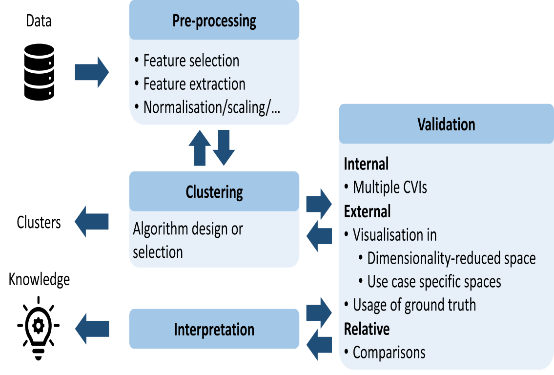
Figure 1: Clustering procedure adapted from Rui and Wunsch (2005). The workflow was iterative and comprised (i) pre-processing, (ii) clustering, (iii) external, internal and relative validation that helped refine the selection of pre-processings, clustering methods and hyperparameter settings, and (iv) interpretation within the respective context leading to (new) knowledge.

2.3 Validation

Validation can generally be categorized into internal and external approaches. Sometimes relative validation is listed as a third option referring to the comparison of different models (Rui and Wunsch, 2005). Internal validation exploits information available during the modelling process. In particular for clustering, Cluster Validity Indices (CVIs) or “scores” provide information on how cohesive a cluster is within itself and how separate it is to other clusters. Here, the Calinski-Harabasz (CH, Caliński and Harabasz (1974)), Davies-Bouldin (DB, Davies and Bouldin (1979)) and Silhouette (SH, Rousseeuw (1987)) scores (Python library scikit-learn, version 1.4) were computed to determine hyperparameters and compare performance. Desirable high within-cluster cohesiveness and between-cluster separation is indicated by low DB and SH and by a local or global maximum of CH.

External validation is achieved by additional knowledge, such as ground truth labels or domain expertise. For biogeochemical and physical clustering, basic principles can be used to evaluate the cluster sets in their 3d geographic space as well as in their temperature-salinity (TS) space. Visual cluster examination can also be conducted in a dimensionality-reduced feature space to assess compliance with feature topology.

2.4 Post-Processing and Uncertainty Assessment

This work addressed uncertainty of the dimensionality reduction by computing the UMAP embedding 100 times and by comparing the similarity between runs using the root mean-squared error (RMSE). For hyperparameter tuning, uncertainty was taken into account by computing each hyperparameter combination ten times for each experiment (see Section 3.2). To quantify uncertainty of DBSCAN, it was applied 100 times to a fixed embedding. The overlap measure (Manning et al., 2008) served as a similarity metric. For uncertainty analysis of the final clustering method, UMAP followed by DBSCAN, the complete embedding-clustering pipeline was executed 100 times. The runs were combined into a final set of clusters using Native Emergent Manifold Interrogation (NEMI; Sonnewald (in review)), whose inherent uncertainty quantification and overlap were used to assess reproducibility. Computational feasibility determined the number of iterations. For more details on uncertainty sources and quantification methods see Supplementary Material C.

3 Results

3.1 Embedding using UMAP

As an initial validation step, the influence of UMAP hyperparameters was tested. A lower number of neighbours led to a more curled structure, while a higher number unfolded it (Fig. 2, a-c). Increasing the number of neighbours to more than 20 did not further change the embedding (Fig. 2, c). As expected, a higher minimum distance caused the data points to spread apart further, blurring finer topologies (Fig. 2, e-f). For the final cluster runs, the number of neighbours was set to 20 and the minimum distance to 0 (Fig. 2, b and d) so that the embedding-space, with three dimensions, exhibited a distinct topology.

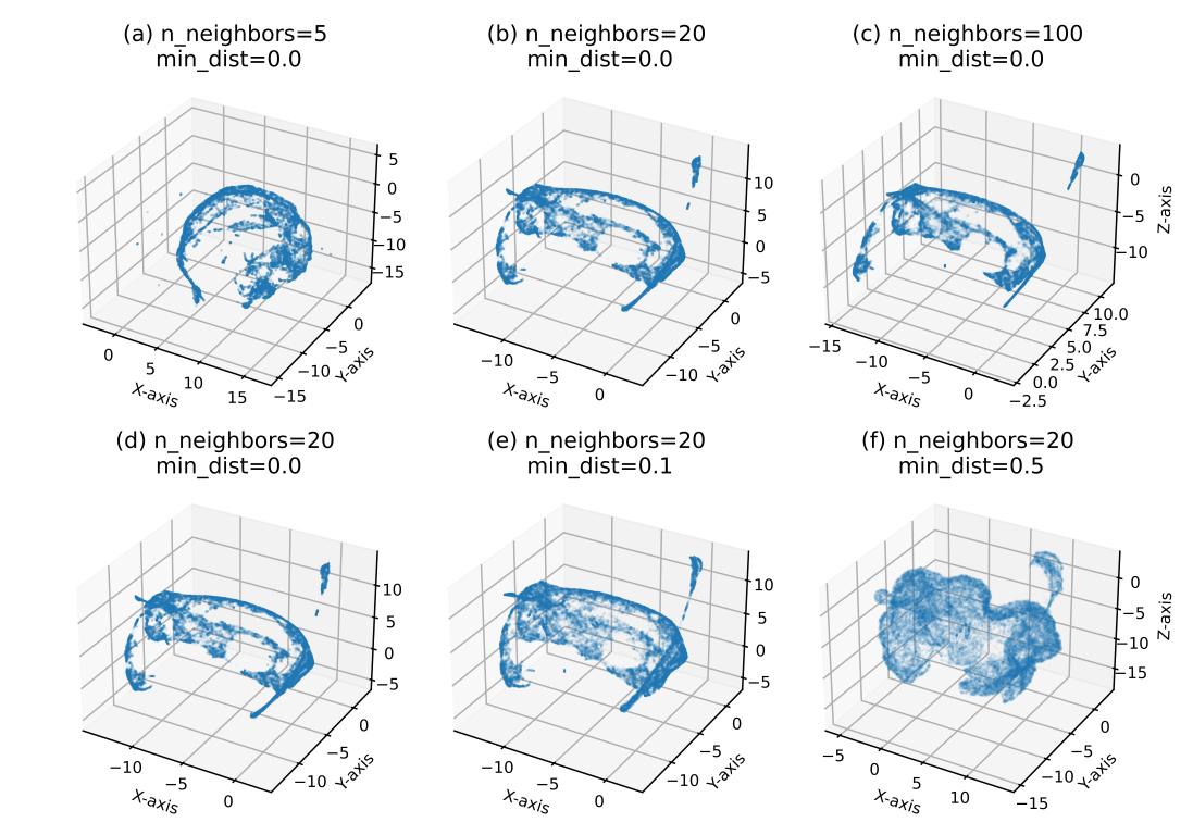
Figure 2: Influence of the UMAP hyperparameters number of neighbours (n_neighbors, top) and minimum distance (min_dist, bottom) on the embedded space. With an increasing number of neighbours, the topology unfolded but did not substantially change for more than 20 neighbours. With a growing minimum distance, the data structure lost structural detail.

3.2 Clustering Results

Six experiments were carried out during which three clustering methods were applied to original and embedded data. Each experiment was run ten times for every hyperparameter combination (Table 1).

Table 1: Overview of clustering results. For external validation, the clustering was visually analysed in geographical and embedding spaces (last two columns, cf. Section 3.2). Note that the Cluster Validity Indexes (CVIs), such as Calinski-Harabasz Score (CH), Davies-Bouldin Score (DB) and Silhouette Score (SH), are not suitable to compare across clustering methods (see Section 4.3). High CH, low DB and high SH indicate a well separated clustering.

Data	Clustering Algorithm	Final Hyperparameters	Internal Validation			External Validation
			CH $\uparrow$	DB $\downarrow$	SH $\uparrow$	Visualisation in Geographic Space	Visualisation in UMAP Space
Original	KMeans	$\textit{n\_clusters}=2$	57,358	0.78	0.5	Warm-cold separation	Division is nearly a straight cut
Embedded	KMeans	$\textit{n\_clusters}=10$	54,457	0.73	0.46	No separation of deep areas	Non-separation of distinct data structures
Original	Agglomerative Ward	$\textit{n\_clusters}=2$	51,825	0.84	0.48	Resembles a hot-cold separation	Intrusions
Embedded	Agglomerative Ward	$\textit{n\_clusters}=23$	64,436	0.72	0.46	Geographically connected	Non-separation of distinct data structures, intrusions
Original	DBSCAN	$\textit{epsilon}=0.11949153$, $\textit{min\_samples}=11$	800	1.44	0.55	Focus on Baltic	Resembles one big cluster
Embedded	DBSCAN	$\textit{epsilon}=0.10661017$, $\textit{min\_samples}=5$	1,818	1.46	$-0.34\text{\,}$	Noisy	Density-oriented, confetti

3.2.1 KMeans

Clustering original data. For KMeans applied to the original 6d data, all three scores reached their peak performance when setting the number of clusters to two (Fig. S5). Plotting the result of KMeans with two clusters in geographic space, two coherent regions emerged (Fig. 3). They most strongly resembled the input temperature distribution, supported by temperature having the highest feature importance ($47\text{\,}\mathrm{\char 37\relax}$). Note that clustering here is not performed on the embedding. The embedding is merely used to visualise how the clusters look like in this space. The visualisation in UMAP space showed clear errors: Structures that are separate were not subdivided, other clusters intruded into foreign clusters.

Higher numbers of clusters resulted in more globular clusters in UMAP space (Fig. S6). Across most clustering levels, temperature and oxygen emerge as the most important features. Meanwhile, the lower-ranked feature of phosphate slightly increased in importance for larger clusters.

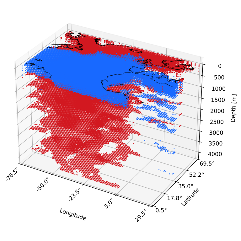
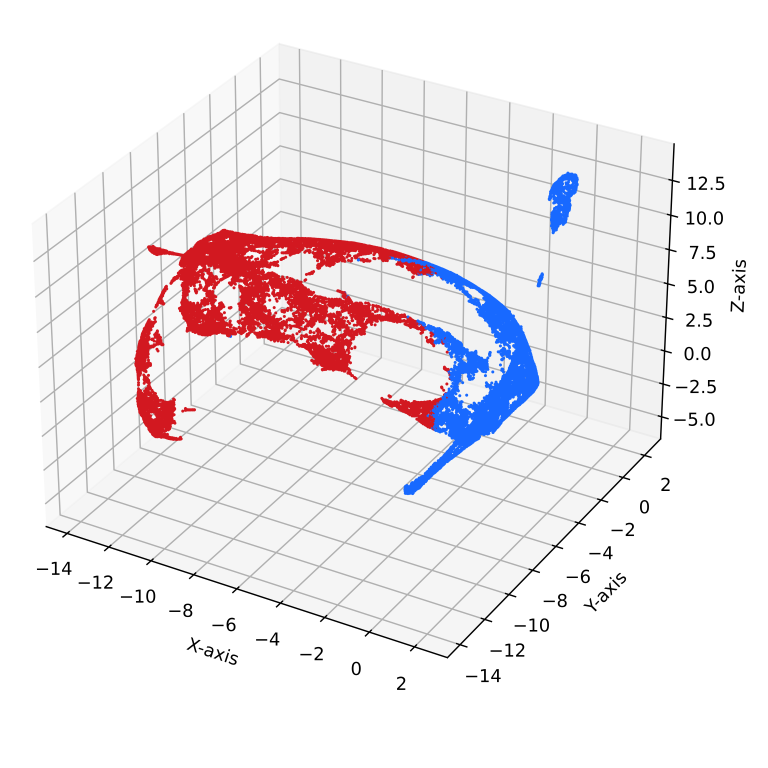
Figure 3: KMeans applied to the original data with two clusters in geographic space (left) and its projection into the embedded space (right). The geographic separation of the clusters resembled the temperature distribution. In UMAP space, the division approximated a straight cut.

Clustering embedded data. For KMeans applied to the data in the previously computed embedded space (Section 3.1), internal validation (the scores) suggested numbers of clusters greater than two (Fig. S5). SH voted for eight clusters and DB for ten, while CH rose beyond the selected value range with a local peak at 13 clusters. The subsequent external validation revealed a more representative clustering as compared to KMeans on original data. However, there were still non-separated regions visible in UMAP space (Fig. 4).

In case that the scores did not detect the proper number of clusters, the cluster sets, generated by varying the number of clusters, were examined by external validation. A higher number of clusters resulted in the embedded space adapting a chessboard pattern (Fig. S7), that was clearly not representative of the underlying co-variance space given by the data.

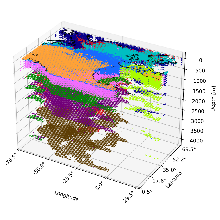
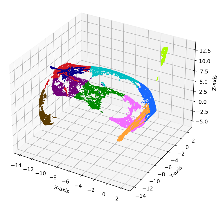
Figure 4: KMeans applied to the embedded data with ten clusters (right) and its projection to geographic space (left). Insufficient performance is reflected in clusters that are not separated despite their clear segregation in UMAP space, e.g. the brown cluster.

3.2.2 Agglomerative Ward

Clustering original data. Similar to KMeans on the original data, all three CVI’s suggested two clusters as the best split using agglomerative Ward clustering (Fig. S8). The visualisation in the embedding revealed a straight cut (Fig. 5) and temperature had the highest importance ($35\text{\,}\mathrm{\char 37\relax}$) followed by oxygen ($34\text{\,}\mathrm{\char 37\relax}$). Increasing the number of clusters up to 30, regardless of the scores, resulted in unseparated clusters and intrusion issues (visible in the embedded space), though less than using KMeans. Temperature contributed most to separation followed by oxygen and salinity.

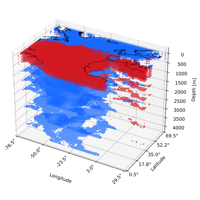
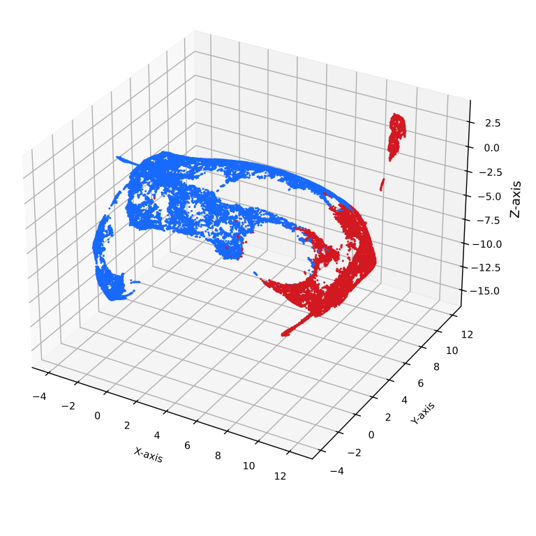
Figure 5: Agglomerative Ward clustering applied to the original data with two clusters (left) and its projection into the embedded space (right).

Clustering embedded data. The scores for agglomerative Ward clustering applied to the embedded data preferred a number of clusters larger than two (Fig. S8). While CH did not show an extreme value that could be used to optimise the number of clusters, DB and SH suggested 24 and 23 clusters as the optimum, respectively. Selecting 23 clusters for less complexity reasonably divided the embedded data at areas of low data point density, except for some smaller clusters (Fig. 6). Deeper ocean regions (two bulbous structures on the left side of UMAP space) and the Mediterranean water masses were well-separated while clustering of original data was not able to find these differences.

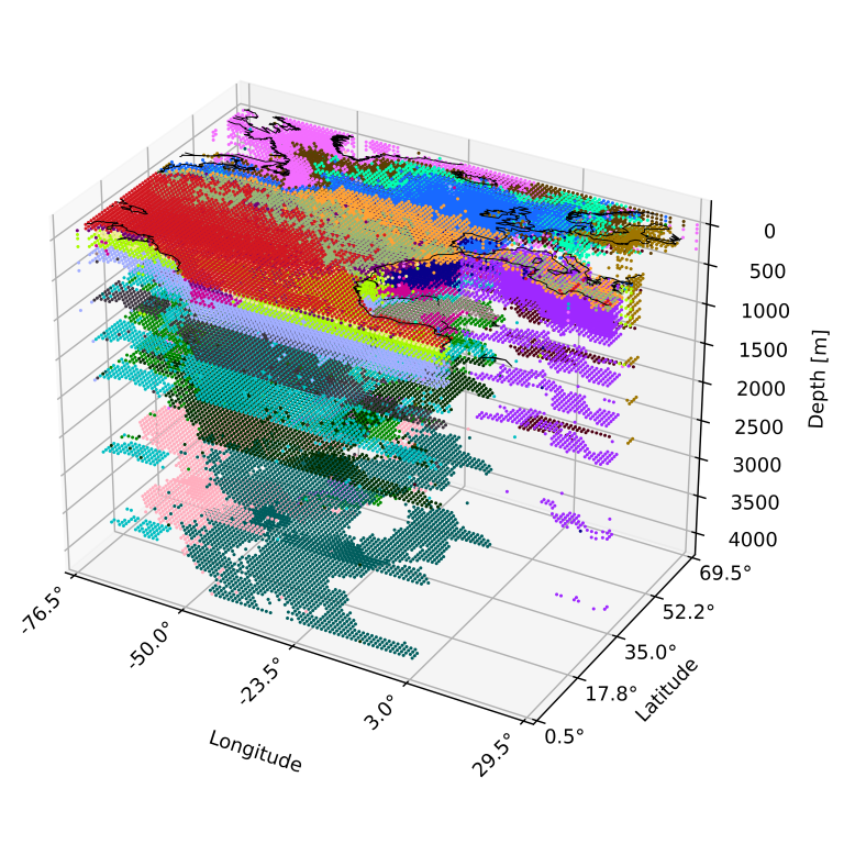
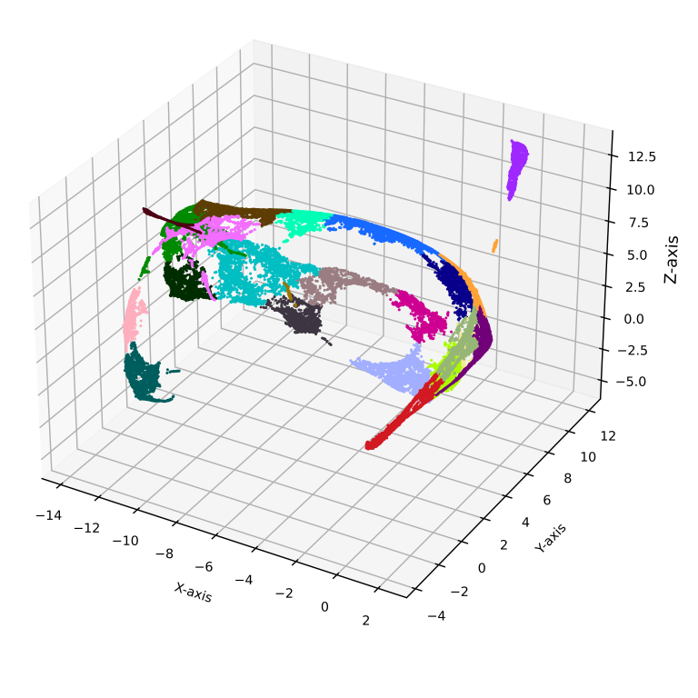
Figure 6: Agglomerative Ward applied to embedded data with 23 clusters (right) and its projection to geographic space (left).

3.2.3 DBSCAN

In contrast to KMeans and Agglomerative Ward clustering, DBSCAN requires tuning of two main hyperparameters: epsilon, i.e., the search radius, and min_samples, i.e., the minimum cluster size. DBSCAN labels data points that it could not assign to a cluster as noise. Therefore, the amount of noise was taken into account for the final choice of hyperparameter settings. For hyperparameter tuning of min_points, values between 2 and 11 and for epsilon values between 0.01 and 0.2 (20 steps with step size 0.00322) were tested for original and embedded data. The number of clusters was considered for hyperparameter selection to prevent an excessive number of regions. For this, the elbow method was applied in the 2d space given by the two hyperparameters, i.e., by selecting the steepest gradient in cluster number in the heatmap (Sonnewald et al., 2020).

Clustering original data. All tested hyperparameter combinations for DBSCAN applied to the original 6d data resulted in similar clusterings that heavily focused on the Baltic, Black and/or Mediterranean Sea (Fig. 7) independent of the tuning criterion (Table ST1). The number of very small clusters or confetti (Section 2.2) decreased with increasing epsilon while higher min_samples led to less confetti and more coherent, but few (mostly below 10) regions.

CH favoured a high min_samples producing a low-noise clustering with coherent regions in the Baltic Sea. DB preferred fewer min_samples and generated a clustering with low noise but spatially less coherent clusters. SH suggested high values for both hyperparameters. Using the number of clusters for the hyperparameter selection resulted in about $34\text{\,}\mathrm{\char 37\relax}$ noise, a lot of confetti and only three larger clusters.

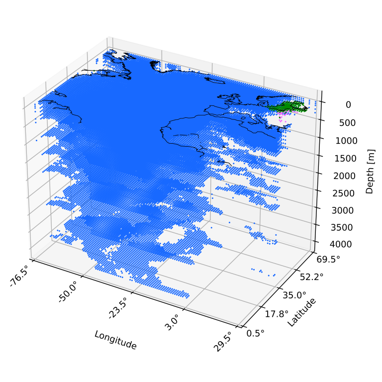
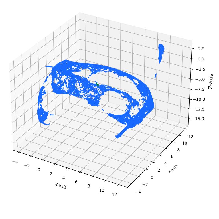
Figure 7: DBSCAN applied to original data (left) and its projection to UMAP space (right). The hyperparameters were selected through the Calinski-Harabasz Score (CH). The clustering was heavily focused on the Baltic.

Clustering embedded data. The distribution of the number of clusters and the noise fraction was similar for DBSCAN applied to the embedded data compared to original data. However, the number of clusters rose above 6,000 and the noise reached proportions of $99\text{\,}\mathrm{\char 37\relax}$. Low epsilon and high min_samples generally resulted in highest noise. Low epsilon and low min_samples led to a large number of clusters (confetti), while an epsilon value above 0.1 generated larger, coherent structures.

The CH (Fig. 8) formed a clear ridge that rose linearly with increasing min_samples. It separated very coarse cluster sets (above the ridge, i.e., larger epsilon values) from cluster sets consisting of smaller regions and increasing confetti (below the ridge, i.e., smaller epsilon). The score hence delineated a compromise between coarse and fine cluster sets. Its optimal/maximal value (at $epsilon=0.16135593$, $min\_samples=11$) produced a cluster set that incorporated clearly delineated regions in geographic and embedded space. In the embedded space, some larger structures were not subdivided despite only thin connections, such as a geographic region in the north. The SH resembled the CH only favouring lower epsilon and min_samples resulting in more confetti. In contrast, the DB preferred hyperparameter combinations producing much noise.

Final hyperparameters were selected based on CH as well as external validation, i.e., the visual inspection of embedded and geographic space. CH was used as orientation since it reflected the trade-off between confetti versus larger coherent regions. The other scores were ignored due to their lack of agreement with visual clustering quality, i.e., they favoured cluster sets with more noise and/or confetti. The visual inspection led to the decision of $epsilon=0.10661017$ and $min\_samples=4$ (Fig. 8, red square). Epsilon smaller than the selected value resulted in more confetti while for larger epsilon, clusters tended to merge. A min_samples smaller than four at the selected epsilon formed a larger cluster in the Labrador Sea and more confetti. The clustering for a minimum of five samples was similar, but had more noise ($5.21\text{\,}\mathrm{\char 37\relax}$ versus $3.82\text{\,}\mathrm{\char 37\relax}$). Increasing the min_samples up to 11 resulted in smaller regions.

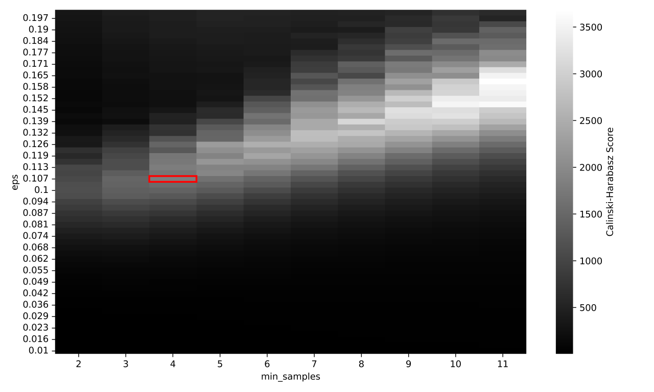
Figure 8: Heatmap showing the Calinski-Harabasz Score (CH) for DBSCAN clustering applied to the embedded data space. Each grid cell represents one cluster experiment carried out with a given combination of the hyperparameters values epsilon and min_samples. The final hyperparameter selection is highlighted by a red square.

3.3 UMAP-DBSCAN: Uncertainty and Post-Processing

Based on the above analysis, DBSCAN applied to the data embedded by UMAP best represented the given data structure. Due to stochasticity of UMAP-DBSCAN, each of the 100 runs produced slightly different results. To assess reproducibility, three sources of uncertainty were examined:

First, UMAP was applied 100 times with the same $n\_neighbors$ and $min\_dist$ to the scaled input data. It was not possible to directly compute the Root Mean Squared Error (RMSE) between any two embeddings since they were not always spatially aligned. Therefore, the point clouds of the embeddings were aligned through manual translation, rotation and/or mirroring followed by the application of the Iterative Closest Point (ICP, Python library simpleicp, version 2.0.14) algorithm to maximise alignment. ICP calculates a translation and rotation matrix for one point cloud trying to minimise distances to another point cloud. The RMSE was computed for the embeddings before and after applying ICP. The minimal deviation, i.e. the error when two embeddings aligned best, was stored, resulting in an average RMSE of $0.22\pm 0.06$ (or about $1.3\pm$$0.36\text{\,}\mathrm{\char 37\relax}$ of the value range)

Second, variability of DBSCAN was assessed by applying it 100 times to a fixed, pre-computed embedding while keeping hyperparameters fixed. For each run, the training data was shuffled. The mean overlap between the resulting cluster sets was $99.99\pm 0.003\%$.

Third, variability of the combined UMAP-DBSCAN pipeline was assessed by running it 100 times, i.e., in each iteration both, the embedding and the clustering, were recomputed. On average, the overlap between the resulting cluster sets was $88.81\pm 1.8\%$ (Fig. S9) .

Native Emergent Manifold Interrogation. To obtain a final cluster set, the statistical variability of the ensemble was exploited by combining the individual members of the 100 UMAP-DBSCAN runs into one cluster set using Native Emergent Manifold Interrogation (NEMI). As base_id, the cluster set with lowest mean NEMI uncertainty was chosen. The final clustering (Fig. 9) had 321 clusters and $3.92\text{\,}\mathrm{\char 37\relax}$ ($n=1,920$) of the grid cells were assigned as noise and were subsequently excluded.

The average NEMI uncertainty (Fig. S10) was $15.49\pm 20\%$ (min: $0\text{\,}\mathrm{\char 37\relax}$, max: $96\text{\,}\mathrm{\char 37\relax}$) and $50\text{\,}\mathrm{\char 37\relax}$ of the uncertainties were $\leq 5\%$. Lowest mean NEMI uncertainties ($0\text{\,}\mathrm{\char 37\relax}$) were found in 6 clusters, three of which were geographically scattered but well separated in embedding space (labels 209, 244, 288). The three certain, geographically cohesive clusters were located in the Black Sea (100 – $2.000\text{\,}\mathrm{m}$; label 93), in the southern Baltic Sea (100 – $400\text{\,}\mathrm{m}$; label 102) and in the Gulf of Saint Lawrence (200 – $1.000\text{\,}\mathrm{m}$; label 112). Uncertainties $\geq 50\%$ were geographically scattered with the exception of a cluster stretching from the Strait of Gibraltar until $-64.5\text{\,}\mathrm{\SIUnitSymbolDegree}$ West (0 – $300\text{\,}\mathrm{m}$; label 28) and a cluster off the coast of North West Africa (200 – $1.500\text{\,}\mathrm{m}$; label 53).

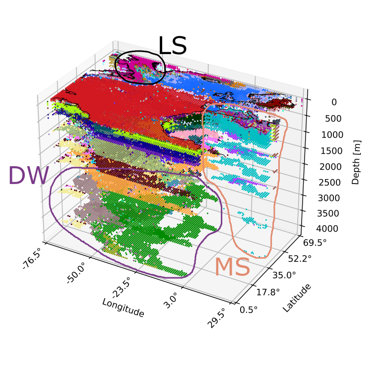
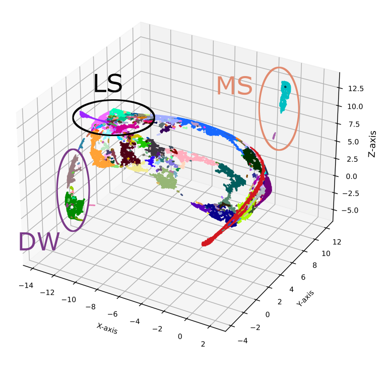
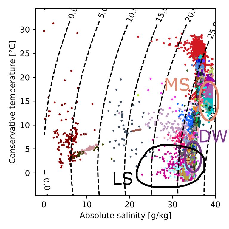
Figure 9: Final UMAP-DBSCAN clustering melted from 100 runs using Native Emergent Manifold Interrogation (NEMI) in geographic (top), embedded (bottom left) and temperature-salinity (TS) space (bottom right). The three use cases (discussed in Section 3.4) are highlighted: Deep Atlantic waters (DW), Labrador Sea (LS) and Mediterranean Sea (MS).

3.4 Case Studies

Three ocean regions from the final clustering, that was based on the combination of 100 UMAP-DBSCAN runs using NEMI (Fig. 9), were inspected.

3.4.1 Mediterranean Sea

In the presented regionalisation, the Mediterranean Sea, delineated by longitude $\in[-6,30]$ and latitude $\in[30,48]$ omitting the Black Sea and Bay of Biscay, had a total of 2,509 grid cells (Fig. 10). The region was subdivided into one large cluster occupying $83\text{\,}\mathrm{\char 37\relax}$ of all cells (label 6), the second largest cluster covering $7\text{\,}\mathrm{\char 37\relax}$ of the grid cells (label 35) and 25 smaller clusters ($<80$ cells) that were mainly found at the surface. Only one larger clusters extended downwards until $100\text{\,}\mathrm{m}$ (label 35, eastern basin).

The main Mediterranean clusters (labels 6, 32, 35, 138) were partly related to the North Atlantic representing the Mediterranean in- and outflow (labels 0, 10, 19, 28) at the Strait of Gibraltar. In TS space, the division between the Mediterranean Sea and North Atlantic waters was clearly visible around the 27-isopycnal. In UMAP space, it was even more pronounced by the large distance between the main Mediterranean cluster (label 6) and the remaining data structure. The clusters representing the Mediterranean outflow were sorted by increasing depth in UMAP space. Highest uncertainties were found in this outflow area (Fig. S11), while the remaining clusters of the Mediterranean Sea had low uncertainty.

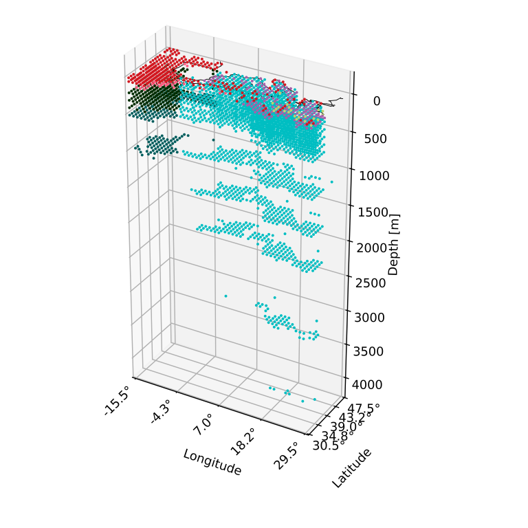
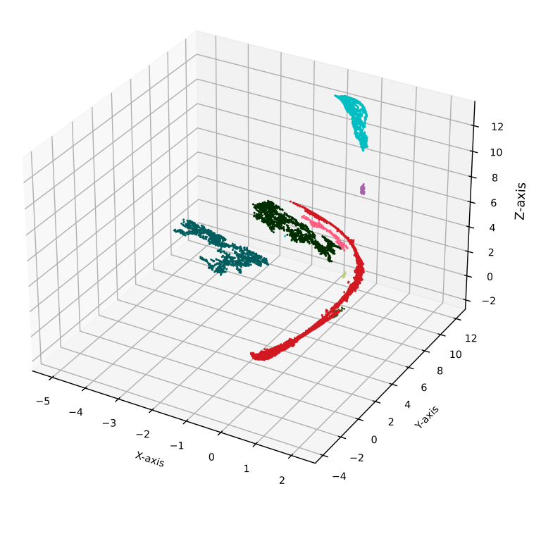
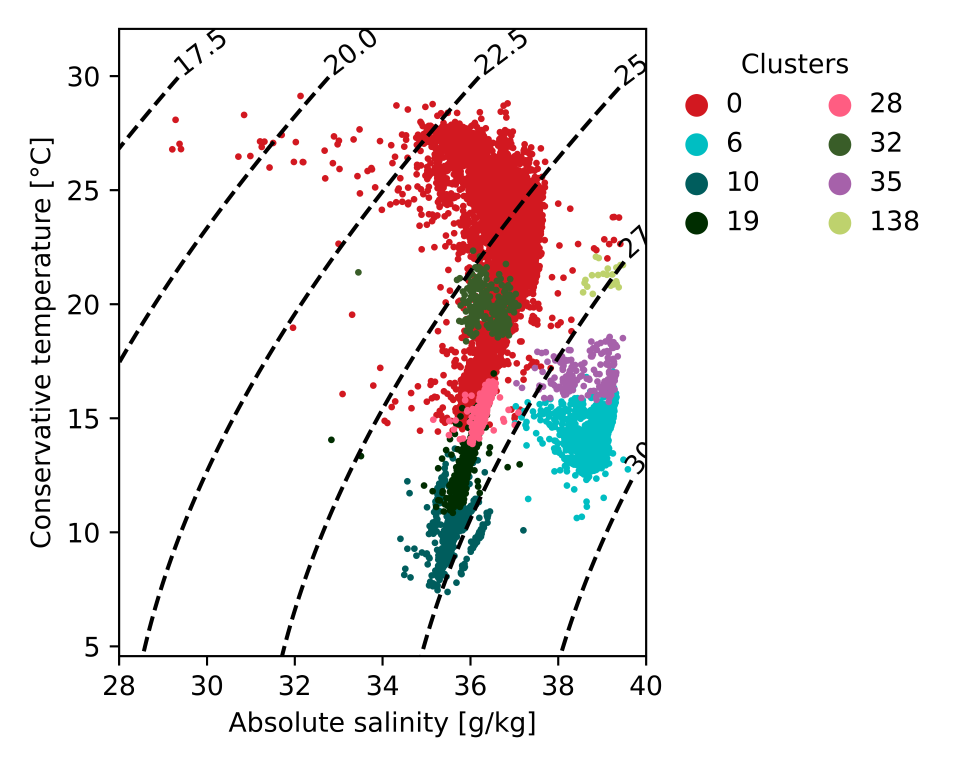
Figure 10: Selected Mediterranean Sea clusters (labels 6, 32, 35, 138) and related in-/outflow regions in the North Atlantic (labels 0, 10, 19, 28) in geographic (left, zoomed into the geographic area of the Mediterranean Sea), embedded (middle) and temperature-salinity (TS) space (right).

3.4.2 Deep Atlantic Waters

The deep waters of the North Atlantic extended from $3.000\text{\,}\mathrm{m}$ to $5.000\text{\,}\mathrm{m}$ stretching over the complete range of considered latitudes and longitudes excluding the Mediterranean Sea. The presented clustering detected 43 clusters (Fig. 11), two of which accounted for the assignment of $79\text{\,}\mathrm{\char 37\relax}$ of the grid cells in that area (labels 2 and 11). 38 clusters had less than 100 cells. Despite having been generally separated by the North Atlantic Ridge, the eastern water mass was also present at the west side of the ridge between 10 and $30\text{\,}\mathrm{\SIUnitSymbolDegree}$. In TS space, these water masses were not distinguishable. For further analysis, six clusters (labels 2, 11, 31, 42, 51, 52) were chosen which had uncertainties below $10\text{\,}\mathrm{\char 37\relax}$, except one in the south-west ($27\text{\,}\mathrm{\char 37\relax}$, label 52, Fig. S12).

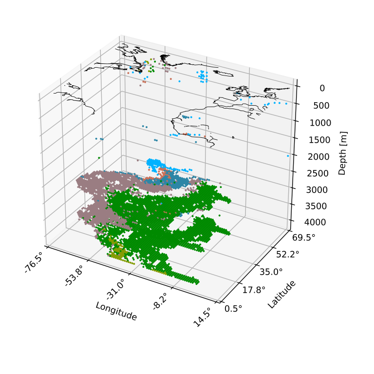
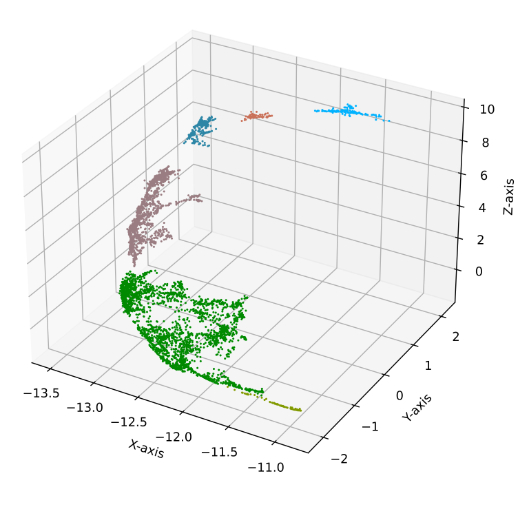
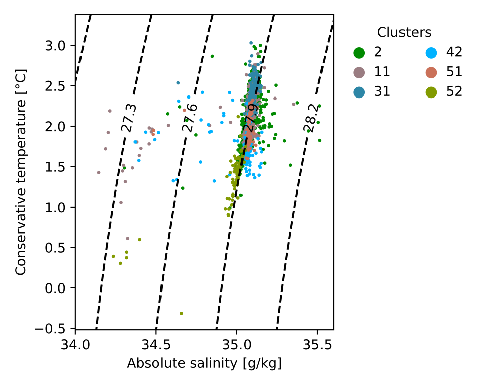
Figure 11: Selected clusters in the deep North Atlantic (labels 2, 11, 31, 42, 51, 52) in geographic (left), embedded (middle) and temperature-salinity (TS) space (right). The clusters were indistinguishable in TS space (except label 50 in the south), but well separable in UMAP space. In geographic space, a division along the Mid-Atlantic ridge was visible.

The east-west separation (label 2 and 11 in Fig. 11) was not clear in TS space but very pronounced in UMAP space (which also considered oxygen and nutrients). Taking a closer look at parameter distributions (Fig. 12) revealed that the western region has notably less silicate and more oxygen as well as lower nitrate and phosphate values.

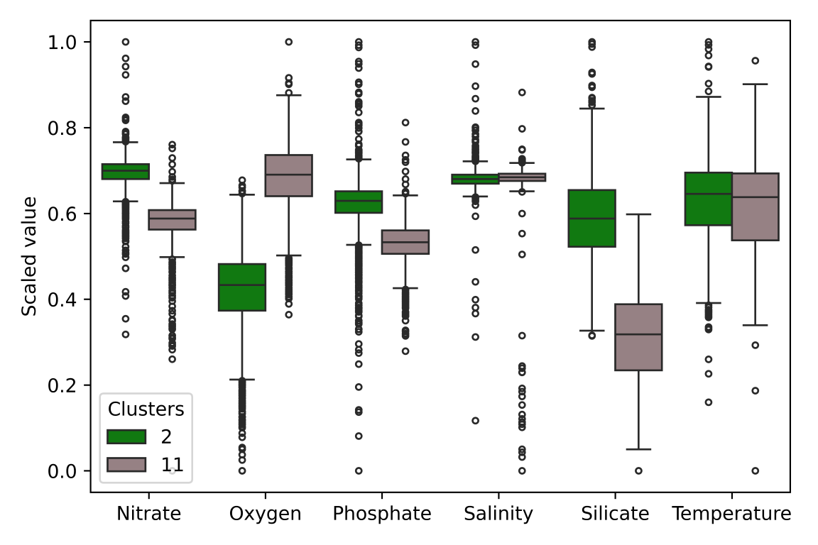
Figure 12: Comparison of parameter statistics of the eastern (label 2) and western deep Atlantic (label 11). Note that the western region had lower nutrient and higher oxygen concentration. The per-parameter differences were statistically significant (p_value$=0$, Mann-Whitney U test, Python library scipy, version 1.11.4).

3.4.3 Labrador Sea and Davis Strait

The Labrador Sea is located between the Labrador Peninsula and Greenland. The Davis Strait between 60 and $70\text{\,}\mathrm{\SIUnitSymbolDegree}$N connects it with Baffin Bay forming a shallower water pathway. 4,170 grid cells were located between 45 and $70\text{\,}\mathrm{\SIUnitSymbolDegree}$N and 40 and $77\text{\,}\mathrm{\SIUnitSymbolDegree}$W, which were assigned to 124 different clusters. The six largest clusters (labels 3, 17, 18, 24, 30, 42, Fig. 13) were analysed, each comprising more than 100 grid cells and the largest having 780 cells (label 17).

The clusters exhibited a strong vertical structure. One cluster (label 17) formed a wide stretch around the surface coasts vanishing at about $300\text{\,}\mathrm{m}$, another one appeared centrally in the Labrador Sea at $50\text{\,}\mathrm{m}$ depth stretching down to $1.000\text{\,}\mathrm{m}$ (label 18). It borders the largest cluster (label 3), which reaches until $3.000\text{\,}\mathrm{m}$ where it is replaced until the bottom by another cluster (label 42). Cluster label 30 filled Baffin Bay from 100 to $400\text{\,}\mathrm{m}$ and was separated from the central cluster (label 18) by an intermediate region (label 24). The latter reached form the surface until $3.000\text{\,}\mathrm{m}$.

The cluster assignment uncertainty (Fig. S13) in this region was on average $10.73\pm 15.4\%$, the median was $4\text{\,}\mathrm{\char 37\relax}$ indicating that uncertainty was inclined towards the lower end. Uncertainties mainly increased along the edges of the embedded data structure, which corresponded geographically to the central area (0 – $500\text{\,}\mathrm{m}$) and an area along the American east coast ($1.500\text{\,}\mathrm{m}$).

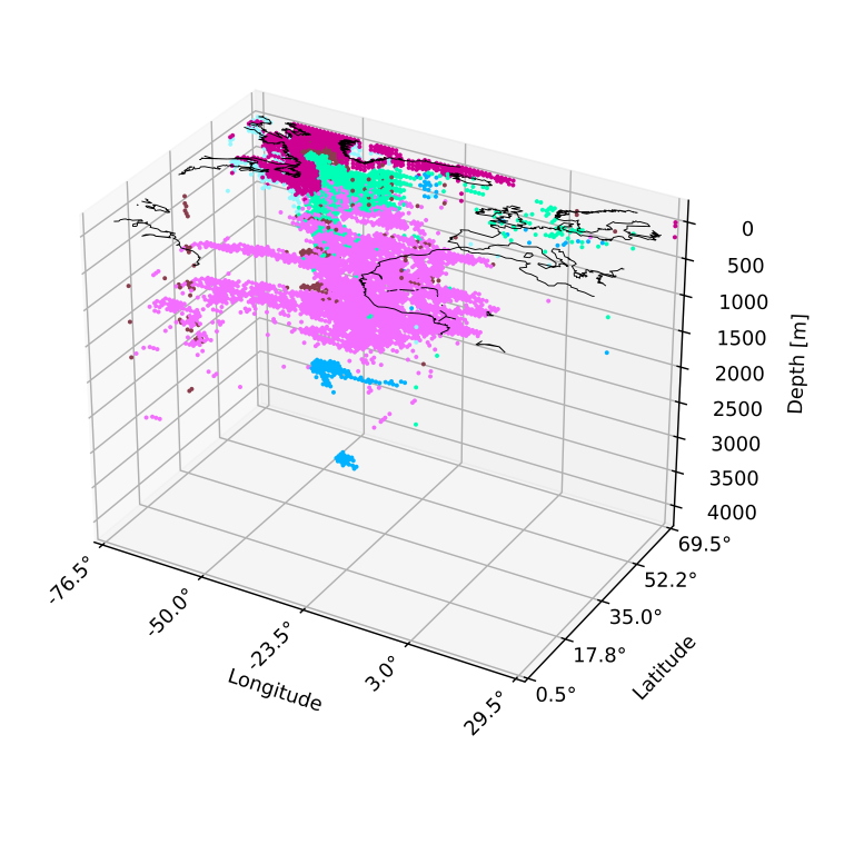
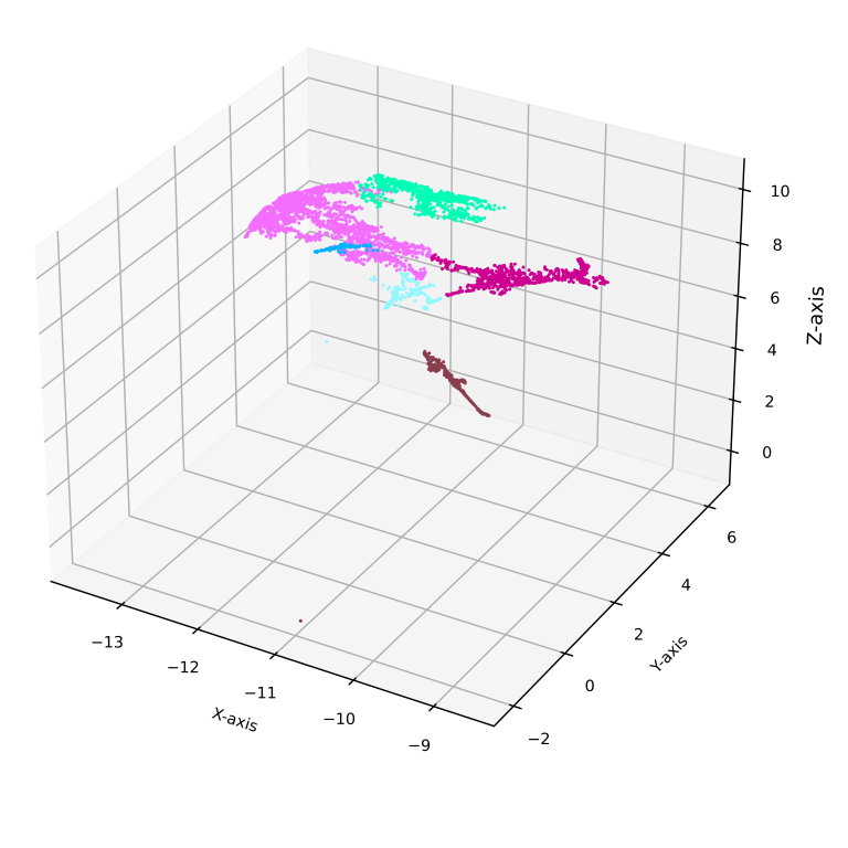
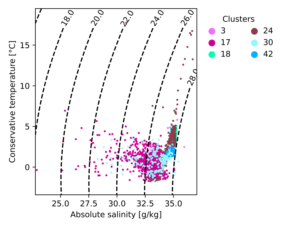
Figure 13: Selected clusters in the Labrador Sea and Davis Strait (labels 3, 17, 18, 24, 30, 42) in geographic (left), embedded (middle) and temperature-salinity (TS) space (right).

4 Discussion

4.1 Comparison of Clustering Algorithm Performance

DBSCAN applied to embedded space created through UMAP best suited the input data. It outperformed KMeans, agglomerative Ward clustering and DBSCAN on original data, as seen in external validation, specifically the visualisation in geographic and UMAP spaces. KMeans and (to a smaller extent) Ward clustering were not able to distinguish small data structures in the embedded space, where clusters were non-separated or merged (Section 3.2). The main reason for the superiority of DBSCAN is its ability to detect clusters of any shape since it operates on data density (Ahmad and Dang, 2015), i.e., it identifies areas where points are concentrated. Also, DBSCAN proved to work well in a similar use case, where it is applied to a dimensionality-reduced data space using t-Stochastic Neighbour Embedding (t-SNE) (Sonnewald et al., 2020). Clusters with varying densities pose challenges for DBSCAN (Ahmad and Dang, 2015), which may explain the occurrence of confetti. Erroneous data could also contribute to this issue.

DBSCAN on original data led to unsatisfactory results, as none of the tested hyperparameter combinations yielded a clustering that reflected the actual data structure, neither in embedded nor in geographic space. The focus on the Baltic Sea, whose salinity levels are well below oceanic average (Tomczak and Godfrey, 2003), is consistent with the feature importances revealing salinity ($35\text{\,}\mathrm{\char 37\relax}$) as the most important feature followed by silicate ($19\text{\,}\mathrm{\char 37\relax}$).

KMeans is a common and fast clustering method and therefore used as a baseline in this work. However, KMeans was not able to reflect the data structure. When applied to the original data, the CVIs agreed on two as the optimal number of clusters. However, the scores cannot be computed for less than two clusters and there is no clustering for less than two clusters. Hence, this result indicated that either (i) two clusters was indeed the best number of clusters or (ii) KMeans could not separate the data structure into relevant clusters or (iii) the scores were not meaningful. For only two clusters, the clustering is mainly a trivial hot-cold separation as seen by the high feature importance of temperature. Mapping the clusters into the embedded space highlighted how KMeans operates, i.e., drawing straight cuts through data structures. Further visual investigation with higher numbers of clusters revealed a tendency to form globular clusters and no increase in clustering quality, i.e., better representation of the embedded data structure.

When applying KMeans to the embedding, the CVIs reached their optimum beyond two clusters. Compared to clustering on the original data, this indicated that KMeans was now better able to detect structures that were also recognized by the scores. However, the scores did not agree: While SH reached its optimum for eight and DB for ten clusters, the DB rose beyond the selected value range. This disagreement emphasised the need for selecting scores carefully and consulting not only one but multiple scores. Still, the clustering exhibited obvious flaws as it could e.g. not distinguish clearly separate structures in UMAP space, such as the deep water. Again, a likely explanation is that KMeans detects spherical clusters best (Ahmad and Dang, 2015; Jain, 2010; Harris and De Amorim, 2022), which were not observed in the embedded space. This clearly indicated that KMeans was not appropriate for the data and might not be for other non-linear use cases either, which are frequent in environmental sciences. Moreover, KMeans is sensitive to the initialisation of cluster centroids (Jain, 2010; Harris and De Amorim, 2022) introducing a variance not investigated in this study.

In contrast to KMeans and DBSCAN, hierarchical clustering provides a complete hierarchy of clusters. In this work, agglomerative Ward detected the overall data structures in UMAP space well (Section 3.2.2) but neglected smaller data point collections. Ward linkage is mathematically close to a KMeans algorithm in a hierarchical context since both methods try to minimise the same objective function, namely the within-cluster-sum-of-squares (Murtagh and Legendre, 2014). It is therefore reasonable that they also had similar score curves.

Regarding post-processing, the combination of the 100 runs from the ensemble into one clustering using NEMI was sensitive towards the $base\_id$ parameter. However, initial experiments showed that the standard deviation of mean uncertainties across runs with different $base\_id$s was only $1\text{\,}\mathrm{\char 37\relax}$. An alternative to NEMI for combining cluster sets from an ensemble are averages over the proximity matrices (whose $ij$-entry is 1 if $i$-th and $j$-th point are in the same cluster, else 0) of a UMAP-clustering pipeline (Bollon et al., 2022). This average is then partitioned using spectral clustering.

For data preparation, further research is required especially for the imputation. Also, density was set to a constant value of $1.025\text{\,}\mathrm{kg}\text{\,}{\mathrm{m}}^{-3}$ for unit conversions as suggested previously (Korablev et al., 2021) when temperature or salinity values are unavailable. Feature importances computed by random forests were only used to get a first impression on the influence of parameters on cluster sets. For a thorough analysis, the models require further tuning and validation.

4.2 The Importance of UMAP Embedding for Clustering Performance

All clustering algorithms performed better when applied to the embedding despite the relatively low dimensional original data space, confirming previous findings (Allaoui et al., 2020; Herrmann et al., 2023). Additionally, the embedded data shows a more balanced feature contribution across all parameters (Fig. S14), reflecting a potentially less biased clustering result. This may lead to clusters that are influenced by multiple factors rather than being driven by a single dominant feature. A possible reason for the performance gain using UMAP is that it enhances separability and thus the ability to cluster data (Herrmann et al., 2023). Moreover, working on a space with fewer dimensions accelerates computation and optimises memory consumption of the given down-stream clustering tasks, and supports external validation by visualisation in the 3d space, where the six original dimensions could not have been used. Working on the embedding helps to overcome the “curse of dimensionality” (Ayesha et al., 2020) that encompasses all phenomena related to higher dimensional data resulting in challenges for learning algorithms. For example, the amount of necessary training data grows exponentially with the number of dimensions to prevent overfitting. Also, Euclidean distances, which are used in all three clustering algorithms, become less discriminative in higher dimensional spaces (Verleysen and François, 2005).

Due to the non-linear nature of the used environmental data, linear dimensionality reduction techniques were discarded such as Principal Component Analysis (PCA), Linear Discriminant Analysis (LDA), Singular Value Decomposition (SVD), Latent Semantic Analysis (LSA), Locality Preserving Projections (LPP), Independent Component Analysis (ICA) and Project Pursuit (PP) (Nanga et al., 2021). Popular non-linear methods include Kernel Principal Component Analysis (KPCA), Multi-Dimensional Scaling (MDS), Isomap, Locally Linear Embedding (LLE), Self-Organizing Map (SOM), Latent Vector Quantization (LVQ), t-Stochastic Neighbour Embedding (t-SNE) and Uniform Manifold Approximation and Projection (UMAP) (Nanga et al., 2021). With the perspective to apply the method to a larger dataset in the future (e.g. by considering a larger geographic area or time as an additional dimension), slow dimensionality reduction methods that do not scale well were omitted (KPCA, ISOMAP, LVQ, t-SNE) (Nanga et al., 2021). SOMs are computationally demanding (Vesanto et al., 2000) and MDS and LLE are sensitive to noise (Nanga et al., 2021) that could be present in the input data. Therefore, UMAP was favoured because it is able to preserve non-linear structures and to scale well.

4.3 Choice and Meaningfulness of Cluster Validity Indices (CVIs)

CVIs for comparing clustering methods did not agree well with external validation. In contrast to the conclusions above, DBSCAN received the worst CVIs for five out of six experiments. The exception was SH, which found DBSCAN on original data the best solution and which was visually the worst subdivision. In four out of six cases, KMeans was classified as the best solution. SH, CH applied to KMeans and DB applied to DBSCAN indicated that the clustering was worse on the embedding than on original data, which conflicted with the previous finding that the clusterings generally benefited from the preceding dimensionality reduction.

All three CVIs used in this study favour clusters of convex shape, a precondition shared by KMeans. It tries to subdivide the data structure into Gaussian regions corresponding to spheres in 3d. Agglomerative Ward is based on an objective function closely related to KMeans, which may explain their similar performance on the clustering and on the scores.

In the used dataset, few convex and many connected clusters with varying shapes were visually found in embedded space questioning the expressiveness of the CVIs for hyperparameter tuning. Since the scores favour a specific type of cluster structure, they are not useful for the comparison of clustering algorithms. Thrun (2021) support this by arguing that instead of selecting a clustering algorithm based on a CVI, the same result would be achieved by directly optimising for that CVI (Thrun, 2021). In practice, the CVIs have nevertheless proven useful in some cases, e.g. CH for DBSCAN tuning. This suggested that the three CVIs can be useful for tuning hyperparameters in non-convex clusters, but should be used with caution.

The selection of CVIs is not trivial and depends on the context and structure of the data. Generally, Arbelaitz et al. (2013) found that overlapping clusters or presence of noise significantly deteriorated performance of the 30 CVIs they investigated (Arbelaitz et al., 2013). Other scores could be tested to tune hyperparameters of the clustering methods, like the Dunn index (Dunn, 1973), WB index (a weighted ratio of sum-of-squares within and sum-of-squares between clusters) (Zhao and Fränti, 2014), I index (Maulik and Bandyopadhyay, 2002), Clustering Validation index based on Nearest Neighbours (CVNN) (Liu et al., 2013), Cluster Validity index based on Density-involved Distance (CVDD) (Hu and Zhong, 2019) or Distance-based Separability Index (DSI) (Guan and Loew, 2020). Each has its own mathematical assumptions about the data (Thrun, 2021). CVDD e.g. claims that it can deal with both spherical and non-spherical clusters. To assess ecological similarity, indices such as the Jaccard and Bray-Curtis indices have been utilized (e.g. Carteron et al. (2012); Sonnewald et al. (2020)).

4.4 Uncertainty Quantification

The uncertainty and reproducibility of the best-performing clustering method (UMAP-DBSCAN) was evaluated using overlap (between all UMAP-DBSCAN runs) and RMSE as a measure. DBSCAN is sensitive to the sequence of input samples (Tran et al., 2013), which was here determined to be negligible (overlap: $99.99\pm 0.003\%$). UMAP uses randomness as it implements stochastic gradient descent for an efficient optimization (McInnes et al., 2018a). With an average RMSE between the data points of the 100 embeddings of 0.22, or $1.3\text{\,}\mathrm{\char 37\relax}$ of the value range, the procedure was assessed reproducible on the given data. The combination of both methods (UMAP followed by DBSCAN) had a mean overlap of $88.81\pm 1.8\%$, corresponding to about $11\text{\,}\mathrm{\char 37\relax}$ uncertainty. Hence, the clusterings were very similar with minor differences. The grid cell-wise uncertainty computed using NEMI amounted to a slightly worse value of $15.49\pm 20\%$. In summary, both, UMAP and DBSCAN, yielded robust and reproducible results alone and in combination.

Uncertainty can be a factor for deciding on a clustering method since a reproducible clustering is often desired. Variance of KMeans and agglomerative Ward was not further investigated, though both methods can differ over multiple runs.

4.5 Relevance for Ecological Interpretations

The biogeochemical clustering approach in our study has strong connections to previous approaches. In comparison to the ecological and biogeochemical regionalisations by Longhurst (2007) and Sayre et al. (2017), the clustering of this study resulted in similar but more detailed clusters with some variation in the spatial extents (Fig. 14). It is obvious that the physical and biogeochemical conditions are closely connected to the characteristics of marine biomes, such as primary production (e.g. Taylor et al. (2011)), microbial diversity (e.g. Friedline et al. (2012)) or cycling of organic matter (e.g. Koch and Kattner (2012); Schmitt-Kopplin et al. (2012); Hertkorn et al. (2013)). For example, the Labrador Sea showed strong similarities across the three clustering sets, though Longhurst (2007) suggested a coarser subdivision. Similarly, Longhurst (2007) and Sayre et al. (2017) identified only one or few regions in the Mediterranean Sea, whereas this study resulted in a total of 27 clusters. This is a result of our strictly data-driven approach, which avoids an arbitrary delineation guided by expert knowledge. Previous studies are based on a priori decisions on the total number of clusters - based on the data or the parameters applied for the clustering method. For example, KMeans (as used by Sayre et al. (2017)) uses a predefined number of clusters and optimises for the entire dataset. This can result in smoothing over local variations, with consequences for the ecological interpretations of the regions. DBSCAN in out study does not enfore a specific number of clusters but prescribes the connectivity conditions, i.e., how far apart data points in feature space may be to form a cluster, which promotes fine-grained subdivisions. In global ecological studies, the Mediterranean is often described as one region (e.g. Longhurst (2007); Costello et al. (2017)) though works like Sayre et al. (2017); Zhao et al. (2020a) and this study suggest a higher diversity especially at the surface in comparison, for example, to the North Atlantic. This is likely caused by complex upper ocean currents (Tomczak and Godfrey, 2003) and small-scale patterns of seasonal primary production (as represented in https://www.grida.no/resources/5937). A short analysis of the proportion of endemic species per region using OBIS data (Ocean Biodiversity Information System (2025) (OBIS), data not shown) revealed $12\text{\,}\mathrm{\char 37\relax}$ of occuring species in the largest and in the second largest Mediterranean clusters (labels 6, 35) to be endemic suggesting the ecological uniqueness of the main biogeochemical water masses in the Mediterranean Sea.

An example for varying region extent in different clustering approaches is the western deep North Atlantic (cluster 11). In this study using DBSCAN and UMAP, the region extended further south along the American coast compared to the Ecological Marine Units by Sayre et al. (2017). By using KMeans, we were able to reproduce the spatial extend in the previous work. The visualisation in UMAP space revealed that KMeans struggled to adequately separate this area. This might be attributable to the complexity of the data, visible in UMAP space as an irregularly connected, curved structure, not resembling normal distributions for which KMeans is optimised. Despite the intrinsic bias of KMeans, the clustering from Sayre et al. (2017) approach and the DBSCAN clustering presented here exhibited many similarities (e.g. surface regions, Fig. 14). A possible reason is that Sayre et al. (2017) use a higher depth resolution: In total, 102 depth intervals were defined and the very variable first $100\text{\,}\mathrm{m}$ of the ocean column are subdivided into $5\text{\,}\mathrm{m}$ steps. This higher resolution might enable a better separation of data points in feature space and thus a more precise clustering.

Generally, the presented cluster set picked up well-known oceanographic features, like the outflow of warm, saline Mediterranean water through the Strait of Gibraltar (Pinardi et al., 2023) that is traceable at the $2.000\text{\,}\mathrm{m}$ level across the North Atlantic Ocean (Tomczak and Godfrey, 2003). Due to the time-averaging of data, small-scale and dynamic oceanographic features such as eddies were not sufficiently represented in this cluster set. Another well-represented feature is the subdivision of deep Atlantic waters along the north-west axis. Compared to the east, the western waters were characterized by lower silicate, nitrate and phosphate and higher oxygen concentration (Fig. 12). This is in good agreement with the fact that the western part of the deep North Atlantic is more influenced by relatively young North Atlantic deep water, while there is more influence of Southern Ocean deep waters in the east (Johnson, 2008). This emphasises that while temperature and salinity remain key parameters in defining water masses, the inclusion of additional parameters such as oxygen and nutrients is crucial for a comprehensive and detailed analysis of water mass properties and dynamics in the ocean.

The clustering results for the case study in the Labrador Sea and Davis Strait, an area of deep-water formation, were generally in very good agreement with pertinent oceanographic literature. Those clusters that represented freshly formed deep water (particularly labels 3 and 24) were characterized by high salinity, low temperature and slightly depleted oxygen values, as shown previously e.g. by Tomczak and Godfrey (2003). The clustering did not always yield spatially coherent clusters, for example a cluster in the deep Atlantic near the equator (label 7). Despite fairly different temperatures, the same cluster label was also assigned to water in the Labrador Sea, because of a high similarity in the inorganic nutrient concentrations. A possible reason is the exclusion of geographic coordinates (or proximity to coasts, such as in Longhurst (2007)) from the clustering process or that additional parameter(s) are required for the distinction.

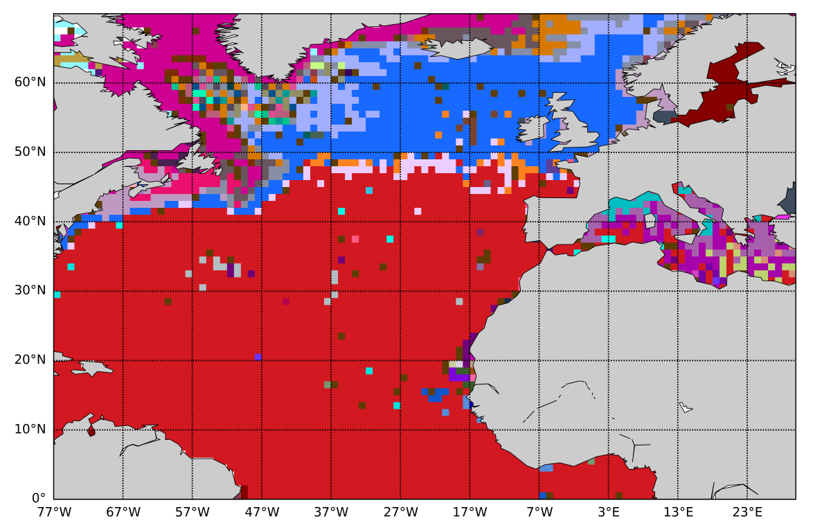
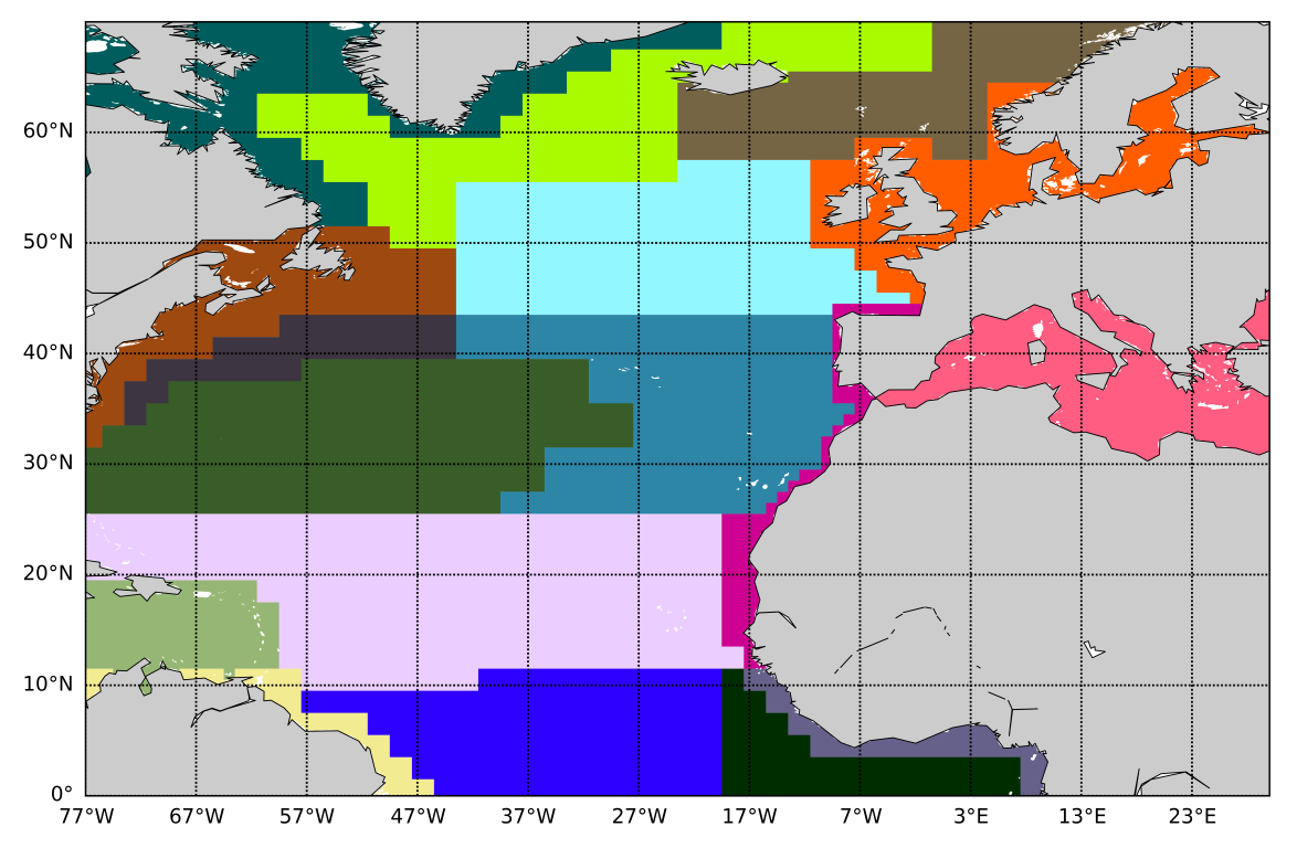
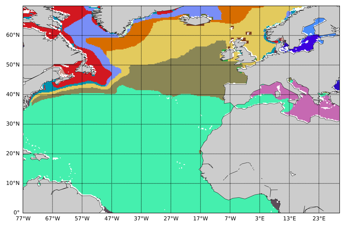
Figure 14: Surface water masses as defined in this study (UMAP-DBSCAN, left), by Longhurst (2007) (middle) and Sayre et al. (2017) (right). While similarities e.g. in the Labrador Sea stand out, there were also differences, such as Longhurst (2007)’s subdivision of the central North Atlantic.

5 Conclusion and Outlook

By comparing pre-processings, clustering methods and various validation techniques, this study found a clustering that adequately reflected the embedded data structure of North Atlantic physical and biogeochemical properties. Such a methodological approach to clustering is of high importance for quality and hence potential downstream tasks. Thrun (2021) formulated this precisely referring to their medical use case:

“[…] only the combination of empirical medical knowledge and an unbiased, structure-based choice of the optimal cluster analysis method w.r.t. the data will result in precise and reproducible clustering with the potential for knowledge discovery of high clinical value.”
— Thrun (2021)

DBSCAN applied to a dimensionality-reduced space using UMAP best reflected the data structure, outperforming KMeans and agglomerative Ward. When validating the results, it was imperative to not rely on single criteria, e.g. to compute multiple CVIs for hyperparameter tuning. The presented results moreover discourage using CVIs for the comparison between clustering methods.

For reproducibility purposes, analysis of uncertainty is an important aspect to consider when non-deterministic algorithms are applied. The variability of the presented method was quantified using ensemble analysis revealing low variabilities of the individual methods (UMAP, DBSCAN) and slight deviations in the clustering when combined (overlap of $88.81\pm 1.8\%$). By combining the clustering results over the ensemble using NEMI, reproducibility and representativeness of the statistical co-variance space was further increased (uncertainty of $15.49\pm 20\%$).

There were several aspects that could be further explored related to data, pre-processing, method and post-processing. Regarding the data, further parameters like dissolved (in-)organic carbon or biogeochemical tracers such as Apparent Oxygen Utilisation (AOU) could be added. We aim to scale the clustering up to global coverage and add the temporal component to increase the benefit for oceanographers. For this, data sparsity could be a problem. Also, other clustering methods that are able to deal with varying densities, such as HDBSCAN, are worth exploring. Also, self-organising maps (Kohonen, 1990) could increase interpretability of results by providing meaningful maps of the classes while preserving data topology (Yonggang and Weisenberg, 2011). To further improve performance, other hyperparameters can be explored. For agglomerative Ward, connectivity constraints could be used to e.g. enforce spatially connected clusters (Camêlo Aguiar et al., 2020). Moreover, distance metrics other than Euclidean could be investigated for Ward and DBSCAN clustering to ensure the optimal strategy for the given data. Oceanographically, the cluster set can be compared more extensively to existing definitions to potentially extract new knowledge.

Acknowledgments
We would like to express our gratitude to the COMFORT project group for their invaluable contribution in providing the dataset that formed the foundation of this research. We are thankful to Claire Monteleoni and Anastase Alexandre Charantonis for their insightful discussions that helped shape the direction of this study. Also, we wish to thank Marlo Bareth for being a valuable discussion partner, whose perspectives helped refine the analysis. YJ was funded through the Helmholtz School for Marine Data Science (MarDATA, Grant No. HIDSS-0005). This work was supported by a fellowship of the German Academic Exchange Service (DAAD), allowing for a research stay of YJ with MS at Princeton University and University of Washington, Seattle. We acknowledge support by the Open Access publication fund of Alfred-Wegener-Institut Helmholtz-Zentrum für Polar- und Meeresforschung.

Data Availability
The cluster set and auxiliary information is publicly available on Zenodo (https://doi.org/10.5281/zenodo.15201767) along with the code base used to conduct and analyse the presented experiments (https://doi.org/10.5281/zenodo.15202343). Column descriptions can be found in Supplementary Material E. The COMFORT dataset is publicly available online (Korablev and Olsen, 2022).

Supplementary Material

Appendix A Data

A.1 Data Preparation

We focused on the North Atlantic and considered a rectangular area extending from $-77\text{\,}$ to $30\text{\,}\mathrm{\SIUnitSymbolDegree}$ longitude, from 0 to $70\text{\,}\mathrm{\SIUnitSymbolDegree}$ and from 0 to $5000\text{\,}\mathrm{m}$ depth. This area had better data coverage compared to the remaining ocean. From the COMFORT dataset (Korablev and Olsen, 2022), we selected the parameters temperature, salinity, oxygen, nitrate, silicate and phosphate, which had best spatial coverage and can serve biogeochemical research questions. The six parameters globally comprised 441,054,314 measured values.

The data was filtered for quality flags provided in the COMFORT dataset. The primary quality flag 1 (PQF1, inherited from the original data sources) was restricted to $>0$ (value was checked) and primary quality flag 2 (PQF2, additional range check) was restricted to $>2$ (acceptable value), which reduced the number of measured values to 313,387,613.

Temperature and salinity values were averaged over identical times and locations (i.e., latitude, longitude, and depth). The averaged salinity and temperature values were joined with the other parameters based on time and location. This enabled the subsequent harmonisation of different units for oxygen, nitrate, silicate and phosphate to $\text{\,}\mathrm{\SIUnitSymbolMicro mol}\text{\,}{\mathrm{kg}}^{-1}$ (Python implementation of Gibbs SeaWater Oceanographic Toolbox of TEOS-10; gsw, version 3.6.17). For the unit conversion, suggestions and formulas from Korablev et al. (2021) were applied. If temperature and salinity values were available, they were used for density computation. Otherwise, density was set to a constant value of $1.025\text{\,}\mathrm{kg}\text{\,}{\mathrm{m}}^{-3}$ as suggested by Korablev et al. (2021). For the oxygen conversion from $\text{\,}\mathrm{\char 37\relax}$ to $\text{\,}\mathrm{\SIUnitSymbolMicro mol}\text{\,}{\mathrm{kg}}^{-1}$, we leveraged formula 31 from Benson and Krause Jr. (1984). This conversion required temperature and salinity values wherefore three oxygen values were discarded. Silicate, nitrate, phosphate and oxygen were averaged over time and location. Temperature was converted to potential temperature (Python library gsw, version 3.6.17) making temperature values from different depths comparable. This procedure resulted in a final set of 306,652,251 measured values.

The six parameters were averaged over all available times (years 1772 – 2020) and mapped on a grid with a spatial resolution of $1\text{\,}\mathrm{\SIUnitSymbolDegree}$ and 12 water depth intervals: 0 – $50\text{\,}\mathrm{m}$, 50 – $100\text{\,}\mathrm{m}$, 100 – $200\text{\,}\mathrm{m}$, 200 – $300\text{\,}\mathrm{m}$, 300 – $400\text{\,}\mathrm{m}$, 400 – $500\text{\,}\mathrm{m}$, 500 – $1000\text{\,}\mathrm{m}$, 1000 – $1500\text{\,}\mathrm{m}$, 1500 – $2000\text{\,}\mathrm{m}$, 2000 – $3000\text{\,}\mathrm{m}$, 3000 – $4000\text{\,}\mathrm{m}$, 4000 – $5000\text{\,}\mathrm{m}$. The depth intervals were roughly aligned with definitions by Sayre et al. (2017) but more coarse to achieve a lower proportion of empty grid cells. We limited the gridded data to latitude in $[0,70]$$\text{\,}\mathrm{\SIUnitSymbolDegree}$, longitude in $[-77,30]$$\text{\,}\mathrm{\SIUnitSymbolDegree}$ and depth in $[0,5000]$$\text{\,}\mathrm{m}$ to achieve good spatial coverage and due to the computational expense. For measurements geographically located on a grid cell boundary, we defined the cells to include values on the lower boundary while excluding values on the upper boundary. The only exceptions were cells with maximum latitude, longitude or depth for which the upper or right boundary was included. To depict a grid cell, we used the horizontal centre and the vertical upper depth boundary, e.g. a grid cell covering $[0,1)$$\text{\,}\mathrm{\SIUnitSymbolDegree}$ $\times[0,1)$$\text{\,}\mathrm{\SIUnitSymbolDegree}$ $\times[0,50)$$\text{\,}\mathrm{m}$ would be labelled [0.5, 0.5, 0].

Grid cells on land were removed from the grid using GEBCO bathymetry information (GEBCO Compilation Group, 2022), resulting in a total of 49,030 grid cells. GEBCO has a resolution of 15 arc seconds, which we downsampled to our $1\text{\,}\mathrm{\SIUnitSymbolDegree}$ resolution by selecting the nearest depth information to each grid cell centre. Downsampling can lead to inaccuracies especially around the coastlines. This means that even though the cell is labelled as land, it can contain a value from a water measurement. Therefore, we only dropped land cells that had no parameter value assigned to it, which also encompassed a few data points that were located further inland.

Grid cells that had values only for a subset or none of the six parameters were filled using K-Nearest Neighbours (KNN, Python library scikit-learn, version 1.4) to achieve a completely specified grid. KNN has two hyperparameters, the number of neighbours, which was set to five and the weights parameter, which was set to “distance”. The six parameters as well as latitude, longitude and depth were scaled to $[0,1]$ and served as input for training the imputer. In total, $3.4\text{\,}\mathrm{\char 37\relax}$ of the grid cells were completely empty, $36.6\text{\,}\mathrm{\char 37\relax}$ were partly empty. Nitrate had the highest proportion of missing values in the grid cells ($35.3\text{\,}\mathrm{\char 37\relax}$), followed by silicate ($26.4\text{\,}\mathrm{\char 37\relax}$), phosphate ($19.7\text{\,}\mathrm{\char 37\relax}$), oxygen ($7.7\text{\,}\mathrm{\char 37\relax}$), temperature ($5.3\text{\,}\mathrm{\char 37\relax}$) and salinity ($3.6\text{\,}\mathrm{\char 37\relax}$). The proportion of missing values for all measurements was $16.4\text{\,}\mathrm{\char 37\relax}$.

A.2 Data Description

The overall average temperature of the prepared data (Fig. S15, top left) was $9.37\text{\,}\mathrm{\SIUnitSymbolCelsius}$, with a minimum of $-1.74\text{\,}\mathrm{\SIUnitSymbolCelsius}$ in the high latitudes and a maximum of $29.83\text{\,}\mathrm{\SIUnitSymbolCelsius}$ at the surface of the Caribbean Sea. Temperature generally decreased with depth, with the exception of the Mediterranean Sea, where warmer waters occurred below the less saline surface layer.

The average salinity (Fig. S15, top middle) was 35.25, with highest values in the Mediterranean (max: 39.49) and in the central area of the North Atlantic, where fluvial input and precipitation is low. Lowest values occurred at the northern coasts, which are influenced by higher precipitation and river run-off (min: 0.05).

The average oxygen concentration (Fig. S15, top right) was $222.4\text{\,}\mathrm{\SIUnitSymbolMicro mol}\text{\,}{\mathrm{kg}}^{-1}$ (min: $0\text{\,}\mathrm{\SIUnitSymbolMicro mol}\text{\,}{\mathrm{kg}}^{-1}$, max: $419.2\text{\,}\mathrm{\SIUnitSymbolMicro mol}\text{\,}{\mathrm{kg}}^{-1}$) with high values at low surface temperatures in the north (due to higher solubility and high primary production in the summer season). The Atlantic subsurface oxygen minimum zone (Karstensen et al., 2008) extends from the west coast of Africa towards South America (blue subsurface layer, Fig. S15).

The average nitrate concentration (Fig. S15, bottom left) was $13.69\text{\,}\mathrm{\SIUnitSymbolMicro mol}\text{\,}{\mathrm{kg}}^{-1}$ (min: $0\text{\,}\mathrm{\SIUnitSymbolMicro mol}\text{\,}{\mathrm{kg}}^{-1}$, max: $315.43\text{\,}\mathrm{\SIUnitSymbolMicro mol}\text{\,}{\mathrm{kg}}^{-1}$) and varied with depth. The surface is nitrate-poor with slightly higher values around Greenland and Iceland and a few exceptionally high values at England’s south coast and the north coasts and estuaries of France and Germany. Higher nitrate values were generally found below the surface, especially at intermediate depths between South America and Africa.

Average phosphate concentrations (Fig. S15, bottom right) were $0.91\text{\,}\mathrm{\SIUnitSymbolMicro mol}\text{\,}{\mathrm{kg}}^{-1}$ (min: $0\text{\,}\mathrm{\SIUnitSymbolMicro mol}\text{\,}{\mathrm{kg}}^{-1}$, max: $7.42\text{\,}\mathrm{\SIUnitSymbolMicro mol}\text{\,}{\mathrm{kg}}^{-1}$. Exceptionally high concentrations occur at the Baltic seafloor, the Gulf of St. Lawrence between $200\text{\,}\mathrm{m}$ and $400\text{\,}\mathrm{m}$, and in the Black Sea (from which only a small region was included in this work). Phosphate showed a strong positive linear correlation with nitrate concentration ($r=0.83$; Fig. S16).

Silicate (Fig. S15, bottom middle) had an average concentration of $13.44\text{\,}\mathrm{\SIUnitSymbolMicro mol}\text{\,}{\mathrm{kg}}^{-1}$ (min: $0\text{\,}\mathrm{\SIUnitSymbolMicro mol}\text{\,}{\mathrm{kg}}^{-1}$, max: $260\text{\,}\mathrm{\SIUnitSymbolMicro mol}\text{\,}{\mathrm{kg}}^{-1}$). The surface was characterised by low values with the main exception being the Labrador Sea and the terrestrially-influenced Baltic Sea. Similar to nitrate, values increased with depth. However, the general correlation between silicate and nitrate/phosphate was weaker ($r\in[0.5,0.6]$; Fig. S16) compared to nitrate and phosphate. At $2000\text{\,}\mathrm{m}$, a large high-silicate area was present at the coasts of Western Europe and Western Africa with values increasing towards the seafloor. Another region of exceptionally high silicate values was located off the west coast of Greenland stretching from $50\text{\,}\mathrm{m}$ down to the sea floor.

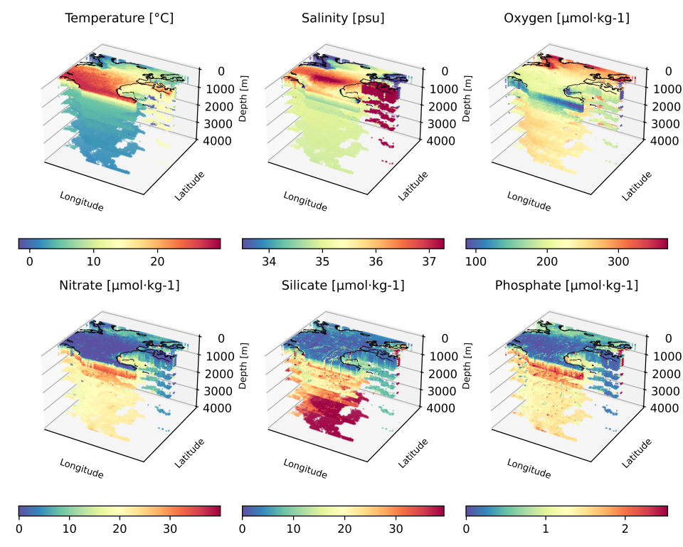
Figure S15: Spatial distribution of the $1\text{\,}\mathrm{\SIUnitSymbolDegree}$ gridded and imputed six input parameters (temperature, salinity, oxygen, nitrate, silicate, phosphate).

Temperature had a Pearson correlation coefficient between $-0.5\text{\,}$ and $-0.6\text{\,}$ with the three nutrients (Fig. S16). Correlations among nutrients ranged between 0.5 and 0.8. All other Pearson coefficients were below 0.5 highlighting that most parameters were not linearly correlated (compare Dickey et al. (2006); Yang et al. (2020)).

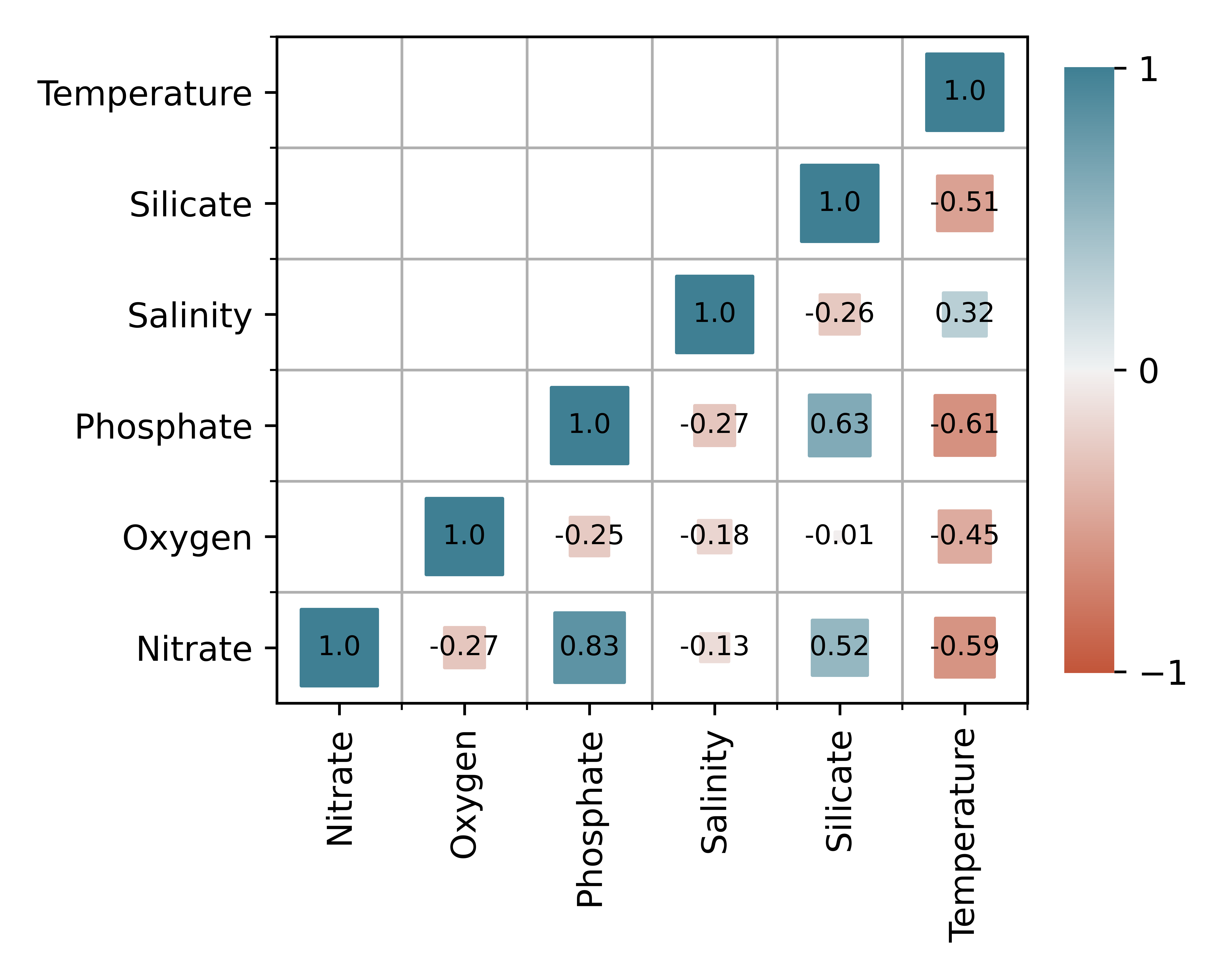
Figure S16: Pearson correlation coefficients between features. Note the moderate to strong correlation between the nutrients, as well as the moderate correlation of temperature with nutrients and oxygen.

Appendix B Method Details

B.1 Dimensionality Reduction: Uniform Manifold Approximation and Projection (UMAP)

Dimensionality reduction is a technique to project data from high to lower dimensionality. It can be classified as a feature selection and feature extraction method (Ayesha et al., 2020). Here we focused on feature extraction, i.e., transforming input features into a new set of features. We applied the non-linear dimensionality reduction technique Uniform Manifold Approximation and Projection (UMAP, McInnes et al. (2018a), Python library umap-learn, version 0.5.5, McInnes et al. (2018b)). UMAP emphasises similarities and differences between data points while keeping the topology. It first represents neighbourhoods by a fuzzy topology, i.e., a high-dimensional graph. Then a low-dimensional graph is constructed to be as similar as possible to the high-dimensional representation by optimising the cross entropy between the two fuzzy sets (Eq. SE2, McInnes et al. (2018a)). The lower-dimensional representation of the data is called embedding.

$$C((A,\mu),(A,\nu))\triangleq\sum_{a\in A}\left(\mu(a)\log\left(\frac{\mu(a)}{\nu(a)}\right)+(1-\mu(a))\log\left(\frac{1-\mu(a)}{1-\nu(a)}\right)\right)$$ (SE2)

where
$(A,\mu)$: Fuzzy set
$A$: Reference set
$\mu\mapsto[0,1]$: Membership strength function

UMAP has two main hyperparameters: The number of neighbours used to compute the high-dimensional representation (n_neighbors) and the minimum distance between points in the low-dimensional space (min_dist). Fewer neighbours lead to a focus on more local structures, while higher values to a focus on more global structures. Increasing the minimum distance shifts the focus from fine to coarse topology in the target space.

B.2 Clustering

A clustering is defined as a function $F$ that maps a set of $d$-dimensional data points $X=\{x_{i}\mid i=1,...,n\}$ to a set of $K$ labels/clusters $\text{Cl}=\{C_{k}\mid k=1,...,K\}$, namely $F:X\mapsto Cl$ (Jain, 2010).

B.2.1 KMeans Clustering

KMeans was introduced independently by various researchers (Ikotun et al., 2023), including Steinhaus (1956), MacQueen (1967) and Lloyd (1982). The default implementation of KMeans (Python library scikit-learn, version 1.4) uses Lloyd’s algorithm, which minimises the within-cluster sum-of-squares and operates in three steps:

1. Select $k$ cluster centroids by default using greedy KMeans++.

2. Assign data points to nearest centroids using Euclidean distances.

3. Update centroids by computing the mean of the assigned data points.

Steps 2-3 are repeated until the centroids do not change more than a threshold (Jain, 2010). The main hyperparameter to tune is the number of clusters $k$.

B.2.2 Agglomerative Clustering

Agglomerative clustering is a type of hierarchical clustering in which the algorithm starts with each data point as a cluster. Then, it successively merges the most similar clusters until only one cluster for all data points remains. The linkage metric determines similarity and thus merging of clusters. Here, we applied Ward linkage (Eq. SE3). It is defined as the sum of squared distances within each cluster and distances between these values for each cluster pair (Ward Jr., 1963):

$$\Delta(C_{i},C_{j})=\frac{|C_{i}||C_{j}|}{|C_{i}|+|C_{j}|}\left\|\text{centroid}(C_{i})-\text{centroid}(C_{j})\right\|^{2}$$ (SE3)

where
$\Delta(C_{i},C_{j})$: Distance between two clusters $C_{i}$ and $C_{j}$ in $Cl$

The clustering proceeds by merging the clusters that are closest according to the linkage (Nielsen, 2016).

B.2.3 Density-Based Spatial Clustering of Application with Noise (DBSCAN)

Density-Based Spatial Clustering of Applications with Noise (DBSCAN, Ester et al. (1996), Python library scikit-learn, version 1.4) groups data according to density: First, neighbours for each data point are detected, i.e., the points that fall into a $d$-dimensional sphere of radius (epsilon) drawn around the initial data point. If this set consists of less than a minimum number of neighbours (min_samples), the central data point is labelled as noise - a label that DBSCAN introduces for data points that it cannot assign. Otherwise, the central point is considered a core point and a new cluster is created. This cluster is expanded by all data points that are found by recursively drawing circles around the member points (Schubert et al., 2017).

Figure S17: An example of a cluster set only consisting of confetti in geographic (left) and in UMAP space (right). It was generated by applying DBSCAN to the embedded data with $\textit{epsilon}=0.01$ and $\textit{min\_samples}=2$.

B.3 Internal Validation

The three scores used in this study are based on different mathematical assumptions and could hence lead to different conclusions. Moreover, all three favour convex clusters. Favouring convexity means that, for example, a clustering with two perfect spheres would result in better scores than a banana-shaped cluster with a cluster in its cavity (Fig. S18).

Figure S18: Convex (left, blue) and concave cluster (right, blue). In a concave cluster it is possible to find two points whose connecting line leaves the cluster. The applied scores (Calinski-Harabasz Score (CH), Davies-Bouldin Score (DB), Silhouette Score (SH)) favour convex clusters, meaning that they would give the left two clusters (blue and grey) a better score than the right two clusters even though the separation is clear in both cases.

Calinski-Harabasz Score. The Calinski-Harabasz Score (CH) or Variance Ratio Criterion (Caliński and Harabasz, 1974) is a measure for within-cluster cohesion and between-cluster disparities. It computes distances to all cluster centres and to the overall data centre:

$$\text{CH}=\frac{tr(B)}{tr(W)}\times\frac{n_{E}-k}{k-1}$$ (SE4)

where $tr(W)$ is the trace of the within-cluster dispersion matrix $W$, which is defined as the sum of within-cluster distances (Eq. SE5)

$$W=\sum_{q=1}^{k}\sum_{x\in C_{q}}(x-c_{q})(x-c_{q})^{T}$$ (SE5)

and $tr(B)$ is the trace of the between-cluster dispersion matrix $B$ (Eq. SE6) that represents the weighted sum of distances between cluster centres and the overall data centre

$$B=\sum_{q=1}^{k}n_{q}(c_{q}-c_{E})(c_{q}-c_{E})^{T}$$ (SE6)

where
$k$: Number of clusters
$n_{E}$: Number of samples in data set $E$
$n_{q}$: Number of points in cluster $q$
$c_{E}$: Centre of data set $E$
$C_{q}$: Set of samples in cluster $q$
$c_{q}$: Centre of cluster $q$

Caliński and Harabasz (1974) recommend selecting an absolute or local maximum in the CH curve or if not present, a comparatively steep increase to decide on a number of clusters. A decreasing coefficient is associated with a possible hierarchical structure of the points. An increasing score indicates clusters that are not well separated. A global/local maximum in the CH curve represents a good balance between within- and between-cluster dispersion, whereas a monotonically increasing CH curve suggests that no partition was better than the one into individual points (Caliński and Harabasz, 1974).

Davies-Boulding Score. Similar to the CH, the Davies-Bouldin Score (DB, Davies and Bouldin (1979)) considers both intra- and inter-cluster Euclidean distances. DB differs from CH by averaging over nearest-cluster similarities instead of taking all cluster centroids into account (Eq. SE7):

$$\text{DB}=\frac{1}{k}\sum_{i=1}^{k}\max_{i\neq j}\frac{s_{i}+s_{j}}{d_{ij}}$$ (SE7)

where
$k$: Number of clusters
$s_{i}$: Mean distance between each point of cluster i and the cluster centroid
$d_{ij}$: Distance between the centroids of cluster i and its most similar cluster j

Small DB indicates better clustering with the minimum value being 0.

Silhouette Score. The Silhouette Score (SH, Rousseeuw (1987)) computes the mean intra-cluster distance $a$ and the mean nearest-cluster distance $b$. Contrary to CH and DB, the SH uses pairwise distances, not centroid distances. The SH for one sample is computed as

$$s=\frac{b-a}{max(a,b)}$$ (SE8)

The SH for the complete clustering averages the SH from each sample. The metric to measure the distance between two data points is Euclidean by default. Besides being higher for convex clusters, this coefficient favours clusters that are dense and clearly separated. SH close to 1 is the best achievable result. Scores around 0 suggest overlapping clusters. Negative values down to $-1\text{\,}$ signify that the data point better fits to another cluster.

B.4 Elbow Method

The elbow or knee method is a well-established subjective heuristic method to balance cost and benefit/performance when altering a system parameter (Satopaa et al., 2011). For example, a Cluster Validity Index (CVI) can be plotted over the number of clusters detected by KMeans, resulting in an L-shaped curve. The elbow of the L-shape indicates a tradeoff between complexity and performance. The elbow concept is transferable to 2d for methods that require two hyperparameters, here for DBSCAN by replacing the elbow curve by a heatmap, in which the elbow was detected as the steepest gradient in the heatmap by computing differences between neighbouring cells.

Appendix C Post-Processing and Uncertainty Assessment

The presented approach was affected by three main sources of uncertainty: (i) data quality and coverage, (ii) missing value imputation and (iii) the pipeline of dimensionality reduction and clustering. Data was filtered using existing quality flags, wherefore data quality was not further investigated in this study. It should be noted though that the COMFORT dataset comprises data measured at different times and with different instruments, which decreases accuracy and precision. Another potential source of uncertainty was the imputation of non-existent measurement values in the defined geospatial grid, which was considered by flagging each imputed data point. Lastly, mapping the original data into the embedding space and the subsequent clustering algorithms comprise a stochastic component leading to uncertainties.

C.1 Cluster Overlap

An asymmetric measure to compare two cluster sets $A$ and $B$ and hence quantify reproducibility is overlap or purity (Manning et al., 2008), which ranges between 0 and 1. It assesses how much the clusters of two cluster sets overlap by calculating the maximum overlap for each cluster/label in $A$ with labels in $B$ and vice versa. The average overlap is used as a cluster set similarity measure.

Let there be $N$ objects that are grouped by clustering $A$ into clusters $a_{0},...,a_{I}$ and by clustering $B$ into clusters $b_{0},...,b_{J}$. The overlap of $A$ with $B$ is then defined as

$$\text{overlap}(A,B)=\frac{1}{N}\sum_{i}\max_{j}|a_{i}\cap b_{j}|$$ (SE9)

To obtain a symmetric measure, we computed the overlap as

$$\text{overlap}=\frac{\text{overlap}(A,B)+\text{overlap}(B,A)}{2}$$ (SE10)

C.2 Native Emergent Manifold Interrogation (NEMI)

Native Emergent Manifold Interrogation (Sonnewald, in review) is a framework that combines clustering with UMAP embedding to compute final cluster labels from an ensemble of partitions. The algorithm requires manual selection of a base cluster set (base_id), against which all other cluster sets are compared. The process begins by matching labels across ensemble members. For this, each cluster set is reassigned new labels sorted by cluster size (with label zero corresponding to the largest cluster). For every member cluster set (except the base), the algorithm visits every possible pair of a base label $a_{i}$ and a member label $b_{j}$ and determines the NEMI overlap as

$$\text{NEMI\_overlap}(a_{i},b_{j})=\frac{\text{volume}(a_{i}\cap b_{j})}{\text{volume}(a_{i}\cup b_{j})}$$ (SE11)

i.e., the volume of geographically shared data points divided by the joint volume of data points. The original NEMI code works with cell count instead of volume.

The ensemble approach also allows uncertainty quantification per grid cell which was computed here as the number of times the cell was assigned to different clusters:

$$\text{NEMI\_uncertainty(grid\_cell)}=100-\frac{|\text{same\_cluster\_assignment}|}{|\text{ensemble}|}$$ (SE12)

In this study, the NEMI approach was used in the final clustering method (UMAP-DBSCAN) to extract cluster labels over an ensemble and determine grid cell-wise uncertainties.

Appendix D Figures for Results and Discussion Sections

Figure S19: Internal validation of KMeans. For clustering the original data (blue), all scores suggest two clusters as the optimal number of clusters. For clustering the embedded data (orange), the scores gave a more clear answer but did not agree on an optimal number of clusters.

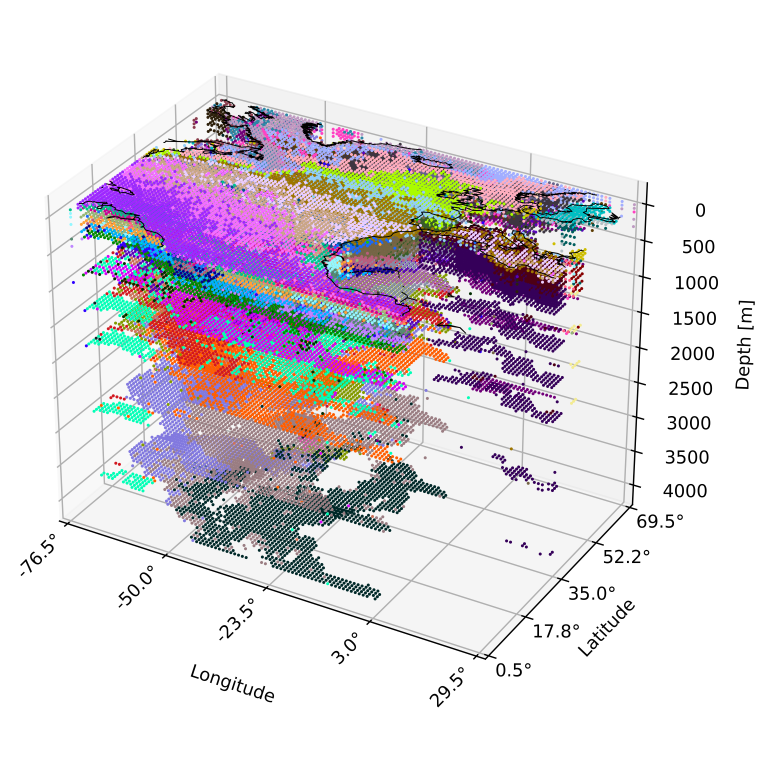
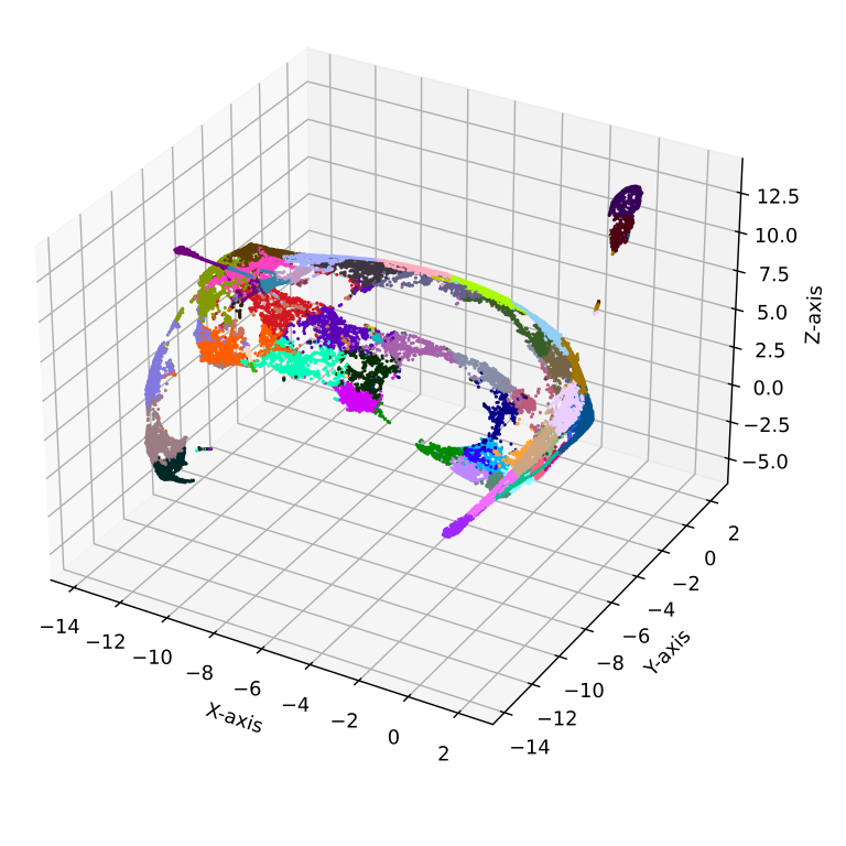
Figure S20: KMeans on original data with the number of clusters set to 60 (left) and its projection into the embedded space (right). A tendency to form convex clusters in UMAP space is visible, clearly not suiting the given data structure.

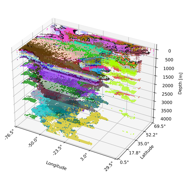
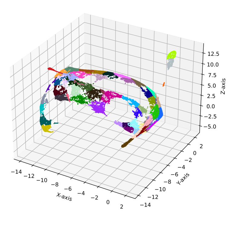
Figure S21: KMeans on embedded data with number of clusters set to 60 (right) and its projection into geographic space (left). The tendency to form convex clusters in UMAP space is even more clear than for KMeans on original data, clearly not suiting the given data structure.

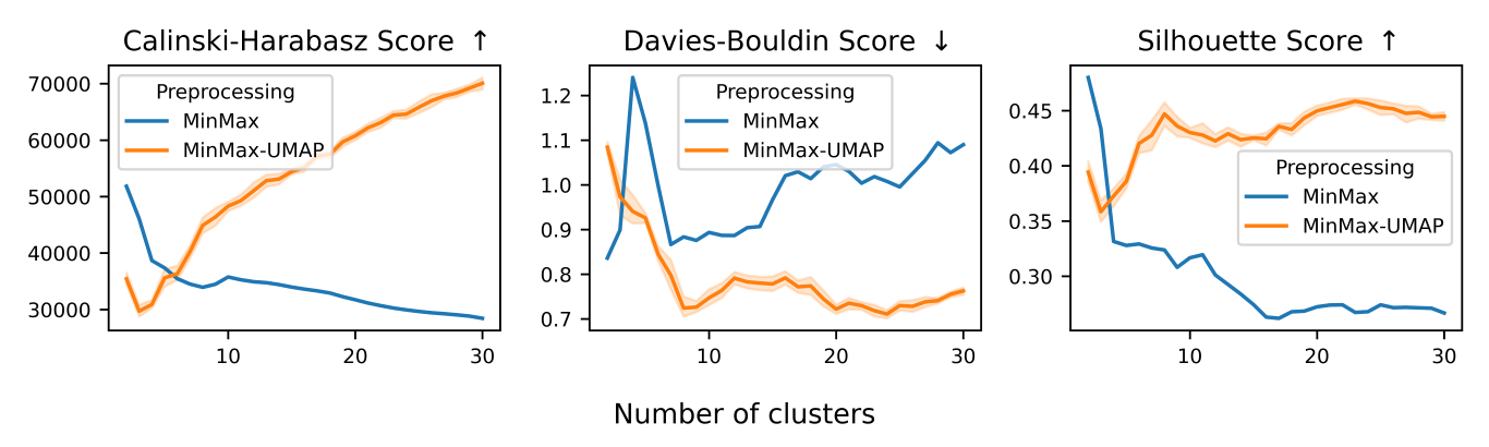
Figure S22: Internal validation of agglomerative Ward. For clustering the original data (blue), all scores suggested two clusters as the optimal number of clusters. For clustering the embedded data (orange), the scores gave a more clear answer but did not agree on an optimal cluster number.

Table ST2: Suggested hyperparameter combinations for clustering with DBSCAN according to the number of clusters, Calinski-Harabasz Score (CH), Davies-Bouldin Score (DB) and Silhouette Score (SH). High CH, low DB and high SH indicate a well separated clustering.

Data	Selection criterion	$epsilon$	$min\_\allowbreak samples$	CH $\uparrow$	DB $\downarrow$	SH $\uparrow$	Number of clusters	Proportion noise grid cells [%]
Original	CH	0.11949153	11	800	1.44	0.55	4	0
Original	DB	0.10338983	3	108	1.08	0.38	12	0
Original	SH	0.2	7	338	1.32	0.58	3	0
Original	Number of clusters	0.01	2	5	1.57	-0.73	2127	34
Embedded	CH	0.16135593	11	3684	1.53	-0.23	110	4
Embedded	DB	0.01966102	7	17	0.95	-0.81	262	93
Embedded	SH	0.04220339	2	35	1.11	0.03	5356	22
Embedded	Number of clusters	0.01966102	2	6	1.04	-0.31	6053	57

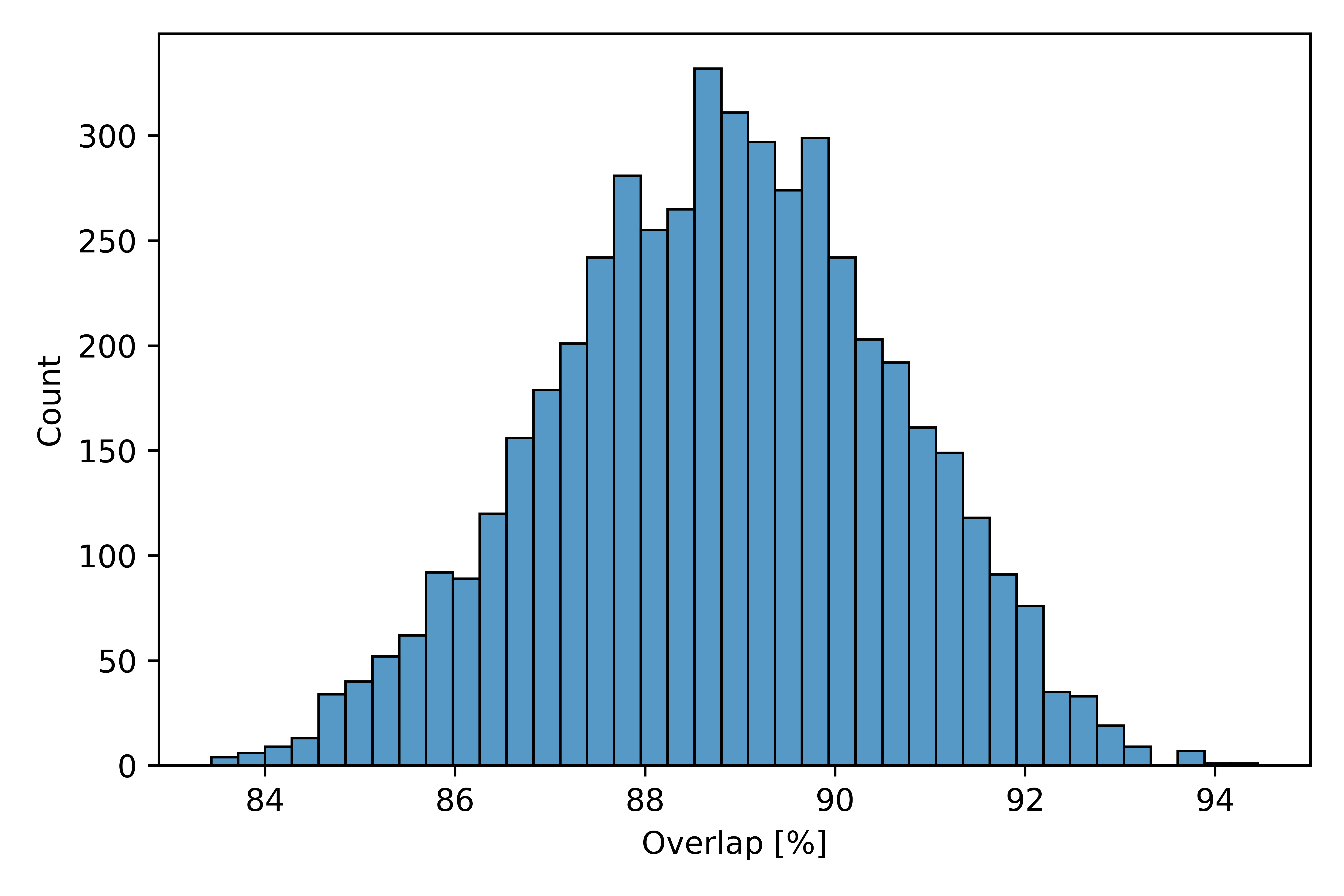
Figure S23: Overlap computed for every pair of clusterings resulting from re-running UMAP-DBSCAN 100 times. The average overlap was $88.81\pm 1.8\%$.

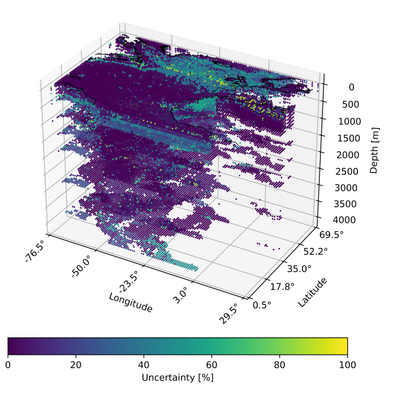
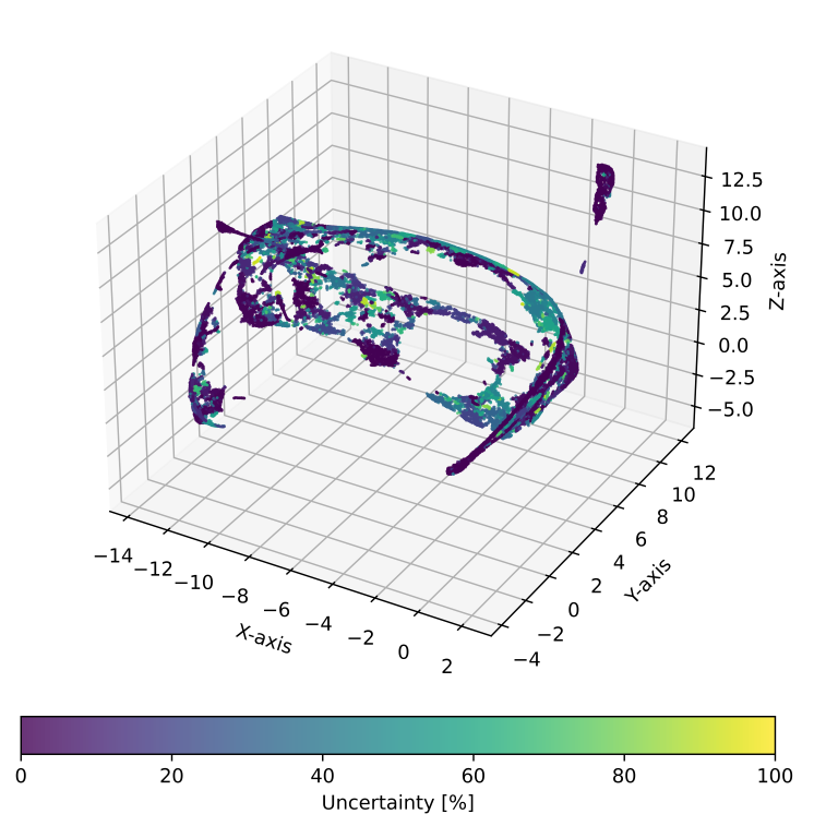
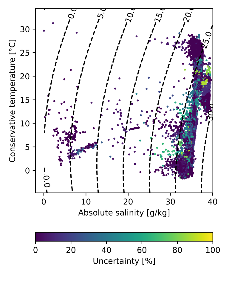
Figure S24: NEMI uncertainty of a UMAP-DBSCAN clustering melted from 100 runs using NEMI in geographic (left), embedded (middle) and temperature-salinity (TS) space (right). The mean uncertainty was $15.49\pm 20\%$ with a median of $5\text{\,}\mathrm{\char 37\relax}$. The high standard deviation and low median indicate a few highly uncertain grid cells skewing the mean.

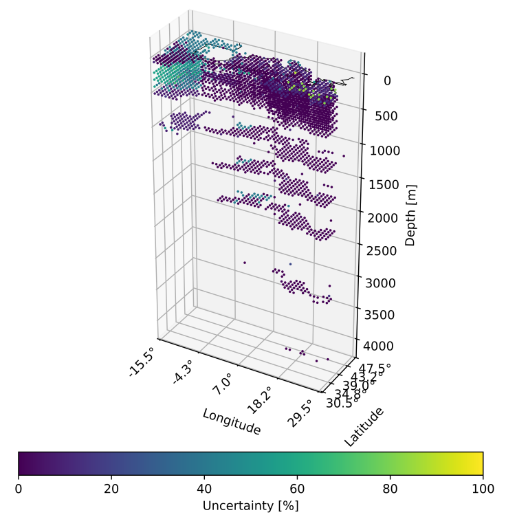
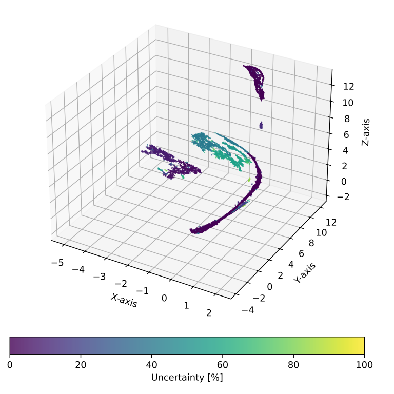
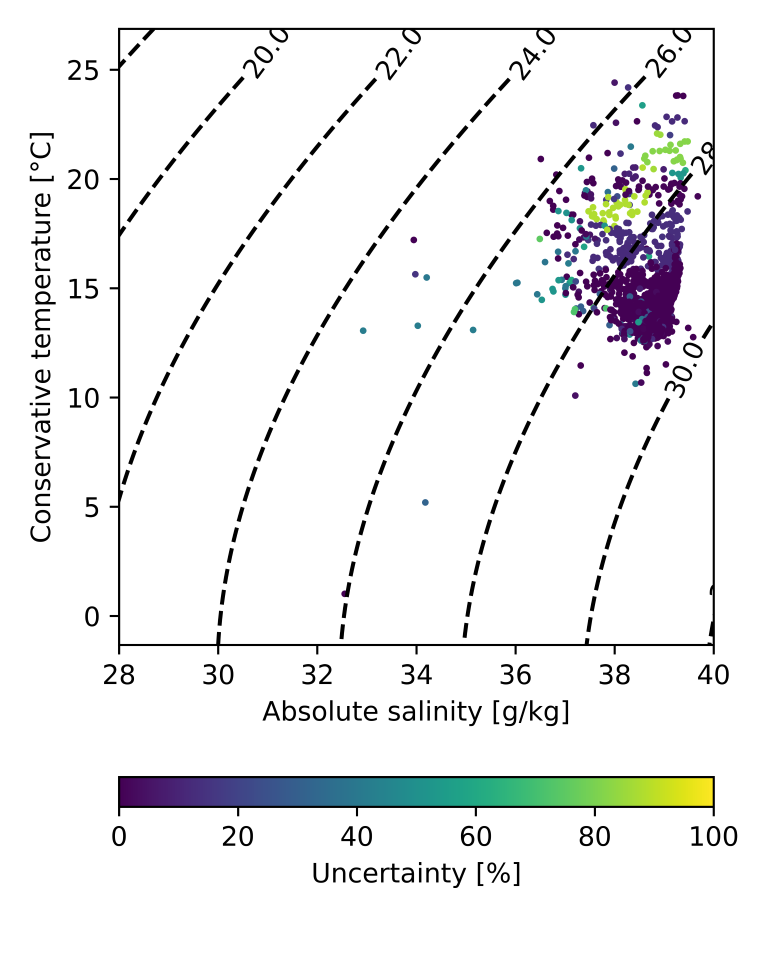
Figure S25: NEMI uncertainty, generated from the variability of the combination of 100 UMAP-DBSCAN runs, of selected clusters in the Mediterranean Sea (labels 6, 32, 35, 138) and its related in-/outflow regions in the North Atlantic (labels 0, 10, 19, 28) in geographic (left, zoomed into the geographic area of the Mediterranean Sea), embedded (middle) and temperature-salinity (TS) space (right). The average uncertainty was $13.08\pm 20.7\%$.

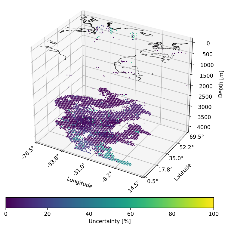
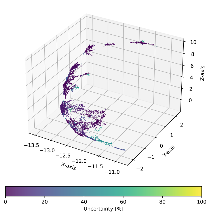
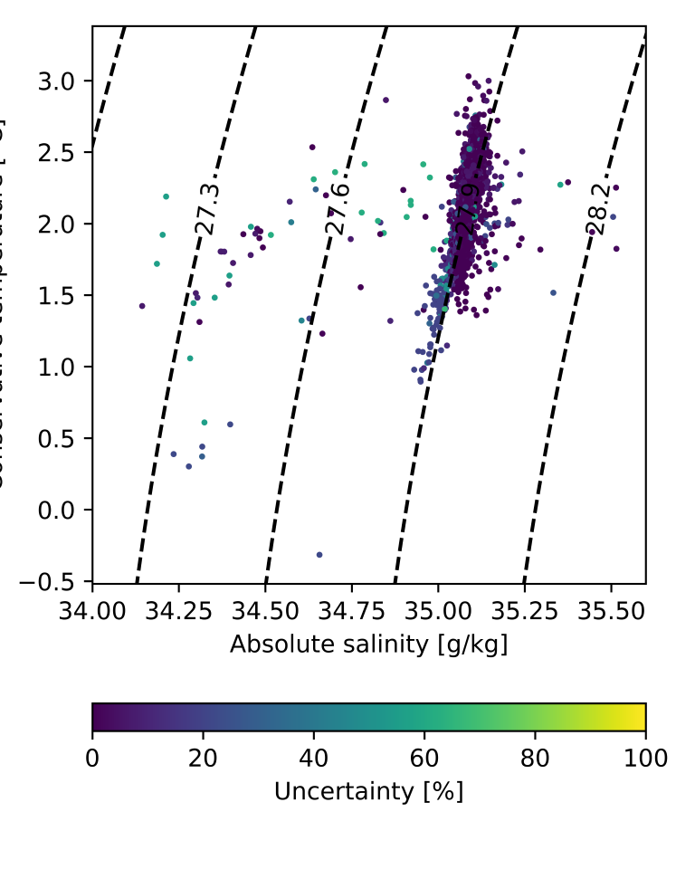
Figure S26: NEMI uncertainty, generated from the variability of the combination of 100 UMAP-DBSCAN runs, of selected clusters in the deep North Atlantic (labels 2, 11, 31, 42, 51, 52) in geographic (left), embedded (middle) and temperature-salinity (TS) space (right). The average uncertainty was $7.74\pm 13.4\%$.

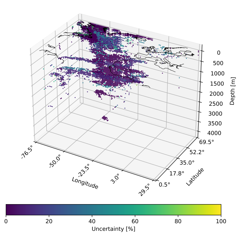
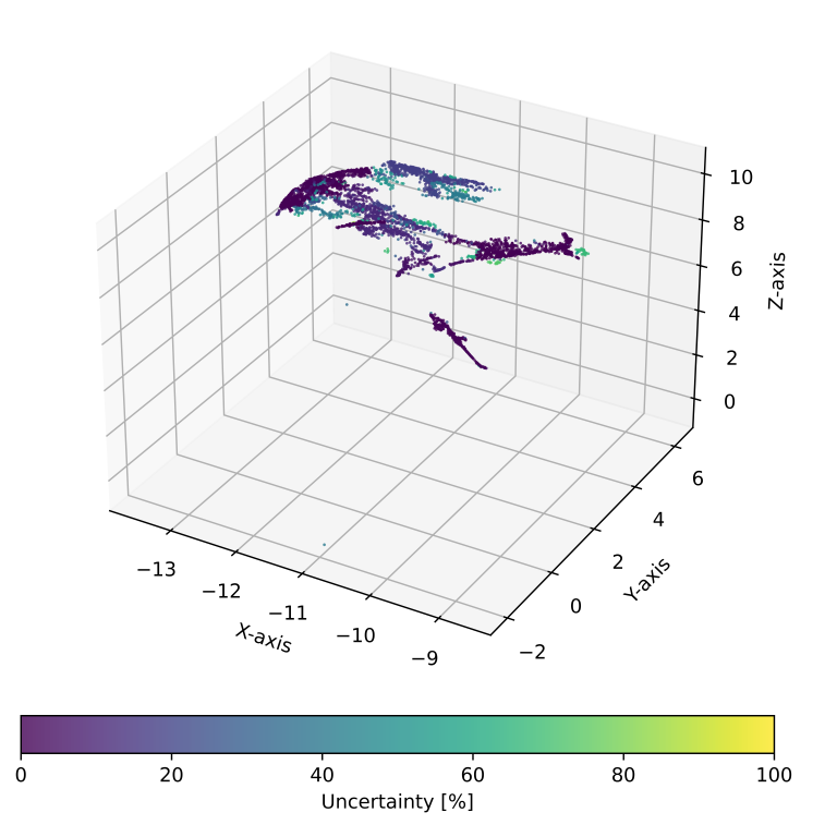
Figure S27: NEMI uncertainty, generated from the variability of the combination of 100 UMAP-DBSCAN runs, of selected clusters in the Labrador Sea and Davis Strait (labels 3, 17, 18, 24, 30, 42) in geographic (left), embedded (middle) and temperature-salinity (TS) space (right). The average uncertainty was $10.73\pm 15.4\%$.

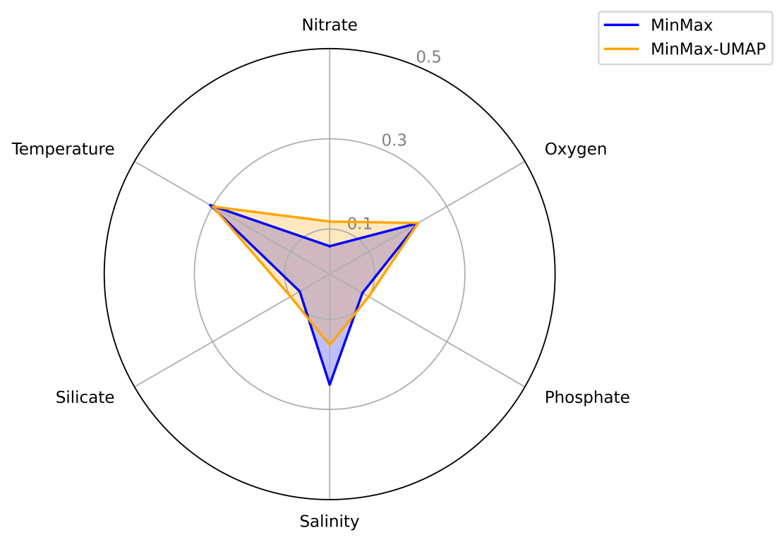
Figure S28: Feature importance of the six input variables averaged over all six clustering experiments revealed temperature, salinity and oxygen as strongest drivers. Clustering embedded data shows a more balanced parameter influence than clustering original data.

Appendix E Cluster Dataset

The final produced clustering (100 UMAP-DBSCAN runs combined into one cluster set using NEMI) is publicly available online (cluster_set.csv). Cluster label eight represents noise as assigned by DBSCAN. The provided file has 18 columns:

1. LEV_M: Upper grid cell depth in $\text{\,}\mathrm{m}$

2. LATITUDE: Geographic latitude of the grid cell centre in decimal degrees

3. LONGITUDE: Geographic longitude of the grid cell centre in decimal degrees

4. P_TEMPERATURE: Average potential temperature of the grid cell in $\text{\,}\mathrm{\SIUnitSymbolCelsius}$

5. P_SALINITY: Average salinity of the grid cell in psu

6. P_OXYGEN: Average oxygen concentration of the grid cell in $\text{\,}\mathrm{\SIUnitSymbolMicro mol}\text{\,}{\mathrm{kg}}^{-1}$

7. P_NITRATE: Average nitrate concentration of the grid cell in $\text{\,}\mathrm{\SIUnitSymbolMicro mol}\text{\,}{\mathrm{kg}}^{-1}$

8. P_SILICATE: Average silicate concentration of the grid cell in $\text{\,}\mathrm{\SIUnitSymbolMicro mol}\text{\,}{\mathrm{kg}}^{-1}$

9. P_PHOSPHATE: Average phosphate concentration of the grid cell in $\text{\,}\mathrm{\SIUnitSymbolMicro mol}\text{\,}{\mathrm{kg}}^{-1}$

10. e0: First reduced feature from UMAP dimensionality reduction

11. e1: Second reduced feature from UMAP dimensionality reduction

12. e2: Third reduced feature from UMAP dimensionality reduction

13. volume: Volume of the grid cell in $\text{\,}{\mathrm{m}}^{3}$

14. label: Cluster label assigned to the grid cell

15. uncertainty: NEMI uncertainty of the cluster label of the grid cell

16. color: Hexadecimal color assigned to the cluster label of the grid cell

17. water: Binary flag denoting if the grid cell is located on land or in water according to GEBCO bathymetry information (GEBCO Compilation Group, 2022)

18. imputed: Percentage of parameters that needed to be imputed for the grid cell, e.g. 50 denotes that $50\text{\,}\mathrm{\char 37\relax}$ = 3 of the six parameters were imputed using KNN

References

- Ahmad and Dang (2015) Ahmad, P.H., Dang, S., 2015. Performance evaluation of clustering algorithm using different datasets. International Journal of Advance Research in Computer Science and Management Studies 3, 167–173.
- Allaoui et al. (2020) Allaoui, M., Kherfi, M.L., Cheriet, A., 2020. Considerably improving clustering algorithms using umap dimensionality reduction technique: A comparative study, in: El Moataz, A., Mammass, D., Mansouri, A., Nouboud, F. (Eds.), Image and Signal Processing, Springer International Publishing. pp. 317–325. doi:10.1007/978-3-030-51935-3_34.
- Arbelaitz et al. (2013) Arbelaitz, O., Gurrutxaga, I., Muguerza, J., PéRez, J.M., Perona, I., 2013. An extensive comparative study of cluster validity indices. Pattern Recognition 46, 243–256. doi:https://doi.org/10.1016/j.patcog.2012.07.021.
- Arnoldi et al. (2023) Arnoldi, N.S., Litvin, S.Y., Madigan, D.J., Micheli, F., Carlisle, A., 2023. Multi-taxa marine isoscapes provide insight into large-scale trophic dynamics in the north pacific. Progress in Oceanography 213, 103005. doi:https://doi.org/10.1016/j.pocean.2023.103005.
- Ayesha et al. (2020) Ayesha, S., Hanif, M.K., Talib, R., 2020. Overview and comparative study of dimensionality reduction techniques for high dimensional data. Information Fusion 59, 44–58. doi:https://doi.org/10.1016/j.inffus.2020.01.005.
- Bailey (1998) Bailey, R.G., 1998. Ecoregions: The Ecosystem Geography of the Oceans and Continents. 1 ed., Springer, New York.
- Benson and Krause Jr. (1984) Benson, B.B., Krause Jr., D., 1984. The concentration and isotopic fractionation of oxygen dissolved in freshwater and seawater in equilibrium with the atmosphere. Limnology and Oceanography 29, 620–632. doi:https://doi.org/10.4319/lo.1984.29.3.0620.
- Bollon et al. (2022) Bollon, J., Assale, M., Cina, A., Marangoni, S., Calabrese, M., Salvemini, C.B., Christille, J.M., Gustincich, S., Cavalli, A., 2022. Investigating how reproducibility and geometrical representation in umap dimensionality reduction impact the stratification of breast cancer tumors. doi:https://doi.org/10.3390/app12094247.
- Briggs (1974) Briggs, J.C., 1974. Maringe zoogeography. McGraw-Hill, New York.
- Briggs (1995) Briggs, J.C., 1995. Global Biogeography. volume 14 of Developments in Palaeontology and Stratigraphy. Elsevier. doi:https://doi.org/10.1016/S0920-5446(06)80051-8.
- Brum et al. (2015) Brum, J.R., Ignacio-Espinoza, J.C., Roux, S., Doulcier, G., Acinas, S.G., Alberti, A., Chaffron, S., Cruaud, C., de Vargas, C., Gasol, J.M., Gorsky, G., Gregory, A.C., Guidi, L., Hingamp, P., Iudicone, D., Not, F., Ogata, H., Pesant, S., Poulos, B.T., Schwenck, S.M., Speich, S., Dimier, C., Kandels-Lewis, S., Picheral, M., Searson, S., Tara Oceans, C., Bork, P., Bowler, C., Sunagawa, S., Wincker, P., Karsenti, E., Sullivan, M.B., 2015. Ocean plankton. patterns and ecological drivers of ocean viral communities. Science 348, 1261498. doi:https://doi.org/10.1126/science.1261498.