On the approximation of the von-Neumann equation in the semi-classical limit. Part II : numerical analysis

Abstract.

This paper is devoted to the numerical analysis of the Hermite spectral method proposed in [14], which provides, in the semi-classical limit, an asymptotic preserving approximation of the von Neumann equation. More precisely, it relies on the use of so-called Weyl’s variables to effectively address the stiffness associated to the equation. Then by employing a truncated Hermite expansion of the density operator, we successfully manage this stiffness and provide error estimates by leveraging the propagation of regularity in the exact solution.

Keywords: Quantum mechanics, von Neumann equation, Hermite polynomial expansion.

1. Introduction

Quantum dynamics exhibits high-frequency waves and requires the numerical resolution of small wavelengths, which presents substantial computational difficulties [2, 13, 19, 22]. Hence, for such problems, it is essential to consider an appropriate mesh strategy, which includes the correlation between time steps, mesh size, and the physical wavelength related to the Planck constant $\hbar$. Similarly, numerical schemes used to solve the Schrödinger equation typically demand that both the time step $\Delta t$ and mesh size, in the semi-classical regime when $\hbar\ll 1$, are of order $O(\hbar)$, or may even be smaller than $\hbar$ [1, 28]. Conversely, time splitting methods have the potential to enhance large time steps when only the physical observables are concerned, as has been shown in [3].

A fundamental concept for understanding these mesh strategies is the Wigner transform, which serves as a useful tool for investigating the semi-classical limit of the Schrödinger equation. In [17], uniform error estimates of time splitting methods have been established for the von Neumann equation in the semi-classical regime. This equation describes the evolution of mixed quantum states, and reduces to the Schrödinger equation in the case of pure quantum states. More precisely, we consider an operator $\hat{\rho}$, called the density-matrix operator, which satisfies the Liouville-von Neumann or simply von Neumann equation, in the operator formulation

$$\left\{\begin{array}[]{l}\displaystyle i\,\hbar\,\partial_{t}\hat{\rho}\,=\,[H,\hat{\rho}],\\[11.00008pt] \hat{\rho}(0)\,=\,\hat{\rho}^{in}\,,\end{array}\right.$$

where $\hbar$ is the reduced Planck constant. The operator $\hat{\rho}$ is acting on the Hilbert space $L^{2}({\mathbb{R}}^{d}):=L^{2}({\mathbb{R}}^{d},{\mathbb{C}})$ equipped with the inner product

(1.1) $$\langle f,g\rangle=\int_{{\mathbb{R}}^{d}}f(x)\,\overline{g(x)}\,\mathrm{d}x\,,$$

and the associated norm of a state to be $\|.\|=\sqrt{\langle.,.\rangle}$. Moreover, the quantum mechanical Hamiltonian $H$ is given, for instance, by

$$H=-\frac{\hbar^{2}}{2m}\,\Delta\,+\,V(X),$$

where $V$ a real-valued function such that $H$ is a self-adjoint operator on $L^{2}({\mathbb{R}}^{d})$. On the other hand, for any $\phi\in L^{2}({\mathbb{R}}^{d})$, $\phi\mapsto V\phi(X)\,=\,V(X)\,\phi(X)$ while

$$[H,\hat{\rho}]=H\,\hat{\rho}-\hat{\rho}\,H$$

is the commutator. Here, we suppose that $\hat{\rho}(t)$ is a density matrix or operator on $L^{2}({\mathbb{R}}^{d})$, such that

$$\hat{\rho}(t)^{*}\,=\,\hat{\rho}(t)\,\geq\,0\,,\quad\text{Tr}(\hat{\rho}(t))\,=\,1,\quad t\geq 0.$$

In particular, $\hat{\rho}(t)$ is trace-class, and therefore Hilbert-Schmidt, hence by [12, Theorem 6.12], there exists a unique function $\rho(t|\,X,Y)\in{L^{2}_{X,Y}:=L^{2}({\mathbb{R}}^{d}\times{\mathbb{R}}^{d},{\mathbb{C}})}$, such that for any $\phi\in L^{2}({\mathbb{R}}^{d})$, we define $\hat{\rho}(t)\phi$ as the function

$$X\,\mapsto\,\hat{\rho}(t)\,\phi(X)\,=\;\int_{{\mathbb{R}}^{d}}\rho(t|\,X,Y)\,\phi(Y)\,\mathrm{d}Y\,.$$

Thus, using this latter representation, the von Neumann equation can be written as follows for the function $(X,Y)\mapsto\rho(t|\,X,Y)$ :

(1.2) $$\left\{\begin{array}[]{l}\displaystyle i\,\hbar\,\partial_{t}\rho(t|\,X,Y)\,=\,-\frac{\hbar^{2}}{2\,m}\,\left(\Delta_{X}\,-\,\Delta_{Y}\right)\,\rho(t|\,X,Y)\,+\,\left(V(X)\,-\,V(Y)\right)\,\rho(t|\,X,Y)\,,\\[11.00008pt] \displaystyle\rho(0)\,=\,\rho^{in}\,.\end{array}\right.$$

First, it is important to emphasize that when $\hbar$ is significantly smaller than $1$, the dynamics governed by the von Neumann equation exhibits stiffness, resulting in a multiscale problem. Consequently, one of the primary challenges in quantum dynamics is the development of efficient numerical techniques capable of describing a diverse range of wavelength amplitudes. For example, we refer the reader to references [21, 31, 32, 33] and the associated literature for discussions concerning the numerical approximation of the Schrödinger equation within the semi-classical limit. Alternative methods based on stochastic algorithms [39] may be also applied in this context.

Furthermore, the density operator associated with the von Neumann equation is defined to be Hermitian, positive semi-definite, and has a trace equal to one, hence preserving these intrinsic properties at the discrete level is crucial to ensure the generation of realistic physical outcomes. In this regard, an initial approach was introduced in [18] which involves the successive application of short-time propagators evaluated using fast Fourier transforms. This method exhibits considerable efficiency for short time intervals, particularly when the density matrix is spatially localized. However, it is worth noting that it necessitates a small time step of the order of $\hbar$ or potentially even smaller. Later in [5], the authors proposed a numerical scheme for a related model, again based on the Fourier pseudo-spectral method. It allows a description both in configuration as well as in momentum space. More recently, various structure preserving schemes have been studied to guarantee trace conservation and positivity of the discrete density matrix allowing long-term simulations.

Recently, we proposed a new approach based on Weyl’s variables to address the stiffness associated with the equation and applied a truncated Hermite expansion of the density operator to manage this stiffness [14]. Actually, this approach is inspired by the link between the von Neumann equation and the Wigner equation, which share the same kind of numerical difficulties arising from the nonlocal and highly-oscillating pseudo-differential operator associated to the potential energy. In [37, 40], it has been shown that the Wigner function can be discretized in a robust way using adaptive pseudo-spectral methods, where the oscillatory components introduced by the Wigner kernel are solved exactly. Finally, the oscillatory quantum effects can also be mitigated by decomposing the potential into classical and quantum parts [35, 36] or by reformulating the Wigner equation using spectral components of the force field [38]. Furthermore, as we will see, the use of Hermite expansion allows for the partial preservation of the operator structure $\hat{\rho}$, which will be helpful in ensuring the stability of this approach.

Our aim here is to analyze the Hermite spectral method proposed in [14], for equation (1.2). We begin by rewriting the von Neumann equation in terms of Weyl’s variables, which eliminates the stiffness associated with $\hbar\ll 1$. The resulting equation is well-suited for the semi-classical limit as $\hbar$ tends to zero (Theorem 1.2). Next, we expand the density matrix using Hermite polynomials, leading to a spectrally accurate approximation. We provide new estimates on the solution of (1.2), demonstrating the propagation of regularity in a weighted Sobolev space. From these estimates, we first derive error estimates in terms of the number of Hermite modes, which are uniform with respect to the parameter $\hbar$ (Theorem 2.1). Additionally, we establish error estimates for the Hermite spectral method applied to the semi-classical limit model (Theorem 2.2). Sections 3 and 4 are dedicated to the proofs of Theorems 2.1 and 2.2. Finally, we perform numerical simulations to illustrate the spectral accuracy of the Hermite method in the last section and refer the reader to [14] for more extensive results.

1.1. Quantum dynamics in Weyl’s variables

To remove the stiffness due to the parameter $\hbar$ in the von Neumann equation, the key idea consists in rewriting (1.2) in the new variables defined below, called “Weyl’s variables”:

(1.3) $$\left\{\begin{array}[]{l}\displaystyle x\,:=\,\frac{X\,+\,Y}{2}\,,\\[8.99994pt] \displaystyle y\,:=\,\frac{X\,-\,Y}{\hbar}\,,\end{array}\right.$$

which can be explicitly inverted as

$$X\,=\,x\,+\,\frac{\hbar}{2}\,y\,,\qquad Y\,=\,x\,-\,\frac{\hbar}{2}\,y\,.$$

Although this terminology is not common, it is obviously suggested by Weyl’s quantization (see formula (1.1.9) of [25]). Hence, we set

$$R(t|\,x,y)\,:=\,\rho\left(t|\,X,Y\right)\,,$$

and find that $\rho$ is solution to (1.2) if and only if $R$ satisfies

(1.4) $$\left\{\begin{array}[]{l}\displaystyle\partial_{t}R(t|\,x,y)\,=\,i\,\sum_{j=1}^{d}\partial_{x_{j}}\partial_{y_{j}}R(t|\,x,y)\,-\,i\frac{V\left(x+\frac{\hbar}{2}\,y\right)\,-\,V\left(x-\frac{\hbar}{2}\,y\right)}{\hbar}\,R(t|\,x,y)\,,\\[11.00008pt] R(0)\,=\,R^{in}\,.\end{array}\right.$$

Let us first review some elementary properties on the function $\hat{\rho}$ and their interpretation in terms of the operator $R$. We first recall that $\hat{\rho}$ is a density operator on $L^{2}({\mathbb{R}}^{2d})$, that is $\hat{\rho}(t)^{*}=\hat{\rho}(t)$, which means that $R$ satisfies

(1.5) $$R(t|\,x,-y)\,=\,\overline{R(t|\,x,y)}\,,$$

whereas the trace property becomes

(1.6) $$\text{Tr}\left(\hat{\rho}(t)\right)\,=\,\int_{{\mathbb{R}}^{d}}\rho(t|\,X,X)\,\mathrm{d}X\,=\,\int_{{\mathbb{R}}^{d}}R(t|\,x,0)\,\mathrm{d}x\,=\,1\,.$$

Translating the positivity condition on $\hat{\rho}(t)\geq 0$ in terms of the function $R$ is more difficult : for all function $\phi\in L^{2}({\mathbb{R}}^{d})$, we have

$$0\,\leq\,\langle\phi|\,\hat{\rho}(t)|\phi\rangle := \iint_{{\mathbb{R}}^{2d}}\overline{\phi(X)}\,\rho(t|\,X,Y)\,\phi(Y)\,\mathrm{d}X\mathrm{d}Y\,,$$

$$= \hbar^{d}\,\iint_{{\mathbb{R}}^{2d}}\overline{\phi(x+\tfrac{\hbar}{2}y)}\,R(t|\,x,y)\,\phi(x-\tfrac{\hbar}{2}y)\,\mathrm{d}x\,\mathrm{d}y\,.$$

We refer to [16] for a characterization of rank-$1$ density operators in Weyl’s variables. Finally, for all $t\geq 0$, we define $\mathcal{S}_{\hbar}(t)$ to be the semi-group associated to the von Neumann equation (1.4) and we have for all $R^{in}\in L^{2}({\mathbb{R}}^{2d})$,

(1.7) $$R(t)\,=\,\mathcal{S}_{\hbar}(t)\,R^{in}\,.$$

By a simple change of variables, we first get the conservation of the $L^{2}$ norm for equation (1.4), hence we have the following proposition.

Proposition 1.1.

Consider $R$ the solution to the von Neumann equation (1.4). Then, we have for each $t\geq 0$,

(1.8) $$\iint_{{\mathbb{R}}^{2d}}|R(t|\,x,y)|^{2}\,\mathrm{d}x\,\mathrm{d}y\,=\,\|\mathcal{S}_{\hbar}(t)R^{in}\|^{2}_{L^{2}}\,\,=\,\|R^{in}\|^{2}_{L^{2}}\,<\,\infty\,.$$

Proof.

On the one hand, since $\hat{\rho}(t)=\exp(-itH/\hbar)\hat{\rho}(0)\exp(itH/\hbar)$ for all $t$, one has

$$\hat{\rho}(t)^{*}=\hat{\rho}(t),\quad\text{ since }\,\hat{\rho}(0)^{*}=\hat{\rho}(0)\quad\text{ and }\quad\mathrm{Tr}(\hat{\rho}(t)^{2})=\mathrm{Tr}(\hat{\rho}(0)^{2})<\infty\,,$$

and it is equally well-known that the Hilbert-Schmidt norm of an operator is the $L^{2}$ norm of its integral kernel, so that

$$\|\rho(t|\cdot,\cdot)\|^{2}_{L^{2}(\mathbf{R}^{d}\times\mathbf{R}^{d})}=\mathrm{Tr}(\hat{\rho}(t)^{2})=\mathrm{Tr}(\hat{\rho}(0)^{2})=\|\rho(0|\cdot,\cdot)\|^{2}_{L^{2}(\mathbf{R}^{d}\times\mathbf{R}^{d})}\,.$$

The simple change of variables (1.3), leading to

$$\|\rho(t|\cdot,\cdot)\|^{2}_{L^{2}({\mathbb{R}}^{d}\times{\mathbb{R}}^{d})}\,=\,\hbar^{d}\|R(t|\cdot,\cdot)\|^{2}_{L^{2}({\mathbb{R}}^{d}\times{\mathbb{R}}^{d})}\;,$$

which yields to the conservation of the $L^{2}$ norm for equation (1.4) : for each $t\in[0,+\infty)$,

$$\iint_{{\mathbb{R}}^{2d}}|R(t|\,x,y)|^{2}\,\mathrm{d}x\,\mathrm{d}y\,=\,\|R^{in}_{\hbar}\|^{2}_{L^{2}}\,<\,\infty\,.$$

∎

This latter property will be crucial in the stability analysis of a numerical method. However, it is not enough to prove convergence, hence we will establish some regularity estimates on the solution to the von Neumann equation (1.4) by propagating moments and derivatives of the solution in $L^{2}$.

1.2. Semi-classical limit

The formulation of the von Neumann equation using Weyl’s variables facilitates the semi-classical limit. Indeed, passing to the limit as $\hbar\to 0$ in the latter equation does not lead to any difficulty related to the stiffness in $\hbar$, since $V\in{\mathscr{C}}^{1}({\mathbb{R}}^{d})$ we have :

$$\frac{V(x+\frac{\hbar}{2}\,y)-V(x-\frac{\hbar}{2}\,y)}{\hbar}\to\nabla V(x)\cdot y,\qquad\text{as }\hbar\to 0\,.$$

Therefore, setting

(1.9) $$\mathcal{E}^{\hbar}(x,y)\,=\,\frac{V(x+\frac{\hbar}{2}\,y)-V(x-\frac{\hbar}{2}\,y)}{\hbar}\,-\,\nabla V(x)\cdot y\,,$$

the function $R$ now solves

(1.10) $$\left\{\begin{array}[]{l}\displaystyle\partial_{t}R(t|\,x,y)\,=\,i\,\sum_{j=1}^{d}\partial_{x_{j}}\partial_{y_{j}}R(t|\,x,y)\,-\,i\left(\nabla V(x)\cdot y\,+\,\mathcal{E}^{\hbar}(x,y)\right)\,R(t|\,x,y)\,,\\[11.00008pt] R(0)\,=\,R^{in}\,,\end{array}\right.$$

where $\mathcal{E}^{\hbar}$ goes to zero as $\hbar\rightarrow 0$. The error made in approximating the solution $R(t|\,x,y)$ of (1.4), or equivalently (1.10), by the solution obtained by neglecting the source term $\mathcal{E}^{\hbar}$, corresponds to the semi-classical limit, given by

(1.11) $$\left\{\begin{array}[]{l}\displaystyle\partial_{t}\hat{R}(t|\,x,y)\,=\,i\,\sum_{j=1}^{d}\partial_{x_{j}}\partial_{y_{j}}\hat{R}(t|\,x,y)\,-\,i\,\nabla V(x)\cdot y\,\hat{R}(t|\,x,y)\,,\\[11.00008pt] \hat{R}(0)\,=\,\hat{R}^{in}\,.\end{array}\right.$$

This limit was made rigorous by P.-L. Lions and T. Paul [26], and P. Markowich and C. Ringhofer [27, 29] for each smooth potential. We also refer to [30, Section 1.4], where an asymptotic expansion of $\mathcal{E}^{\hbar}$ in powers of $\hbar$ is performed for smooth potential. In the following, we define $\mathcal{S}_{0}(t)$, to be the semi-group corresponding to the semi-classical limit equation (1.11), so that

(1.12) $$\hat{R}(t)=\mathcal{S}_{0}(t)\,\hat{R}^{in}.$$

We now restrict ourselves to the one-dimensional case $d=1$ and present an error estimate between the solutions $R(t|\,\cdot,\cdot)$ of (1.4) and $\hat{R}(t|\,\cdot,\cdot)$ of (1.11) in terms of $\hbar$. The key point here is to establish some regularity estimates on the solution to (1.11). To this effect, we introduce the following quantity for any function $R$ and each integer $m\geq 0$

(1.13) $$\mathcal{N}_{m}(t)\,:=\,\sum_{a+b+\alpha+\beta\leq m\atop a,b,\alpha,\beta\in{\mathbb{N}}}\|x^{a}\partial^{b}_{x}y^{\alpha}\partial^{\beta}_{y}R(t)\|_{L^{2}}\,.$$

Let us fix an integer $m\geq 0$ and suppose that the potential $V$ is such that

(1.14) $$V\in{\mathscr{C}}^{m+1}({\mathbb{R}})\quad{\rm with}\quad m\geq 1\quad{\rm and}\quad V(x)\to+\infty,\quad{\rm as}\quad|x|\to\infty\,,$$

and for all $n=2,\ldots,m+1$, there exists a constant $C>0$, independent of $\hbar$, such that

(1.15) $$\|V^{(n)}\|_{L^{\infty}}\,\leq\,C,{\quad{\rm with\,}V^{(n)}=\frac{d^{n}V}{dx^{n}}}\,.$$

We prove the following result.

Theorem 1.2.

Assume that $V$ satisfies (1.14)-(1.15) with $m=3$ while for all integers $a$, $b$, $\alpha$ and $\beta$ such that $a+b+\alpha+\beta\leq 3$, we have

(1.16) $$\left\{\begin{array}[]{l}\displaystyle\|x^{a}\partial^{b}_{x}y^{\alpha}\partial^{\beta}_{y}\hat{R}^{in}\|_{L^{2}}\,<\,\infty,\\ \displaystyle\|R^{in}\|_{L^{2}}\,<\,\infty.\end{array}\right.\displaystyle$$

Then the solution $R$ to the von Neumann equation (1.4) and the solution $\hat{R}$ to (1.11) with the initial data $R^{in}$ and $\hat{R}^{in}$ satisfy

$$\|R(t)\,-\,\hat{R}(t)\|_{L^{2}}\,\leq\,\|R^{in}\,-\,\hat{R}^{in}\|_{L^{2}}\,+\,\mathcal{C}(t)\,\hbar^{2}\,,$$

where $\mathcal{C}(t)$ is given by the following expression

$$\mathcal{C}(t)\,:=\,\frac{1}{24}\,\|V^{(3)}\|_{L^{\infty}}\,\frac{e^{C_{3}[V]\,t}\,-\,1}{C_{3}[V]}\,\mathcal{N}_{3}(0)\,,$$

with $C_{3}[V]$ defined later in (3.1) and $\mathcal{N}_{3}(0)$ is given in (1.13) applied to $R^{in}$.

The proof of this theorem is presented in Section 3. Actually, it is relatively elementary since it is a consequence of a simple Taylor expansion of the potential $V$, but the propagation of regularity of the solution to the semi-classical limit problem (1.11) is required. This will be achieved by studying the functional $\mathcal{N}_{m}(t)$, defined in (1.13), applied to the solution $\hat{R}(t)$ to (1.11). This results can be interpreted as a modulated energy estimate where only regularity on the solution of the limit equation is required (see for instance [4] or [11]).

2. Hermite Spectral method

The purpose of this section is to present a formulation of the von Neumann equation (1.4) written in Weyl’s variables based on Hermite polynomials. We first use Hermite polynomials in the $y$ variable and write the von Neumann equation (1.4) as an infinite hyperbolic system for the Hermite coefficients depending only on time and space. The idea is to apply a Galerkin method keeping only a small finite set of orthogonal polynomials rather than discretizing the operator $R$ in $y$ on a grid. The merit of using an orthogonal basis like the so-called scaled Hermite basis has been shown in [20, 34] and more recently in [7, 6, 10, 9, 8, 15] for the Vlasov-Poisson system. We define a weight function $\omega$ as

$$\omega(y):=\pi^{-1/4}\,e^{-y^{2}/2}\,,\qquad y\in{\mathbb{R}}\,,$$

and the sequence of Hermite polynomials (called the “physicist’s Hermite polynomials”) by

$$H_{k}(y)\,=\,(-1)^{k}\,\omega^{-2}(y)\,\partial_{y}^{k}\omega^{2}(y)\,,\qquad k\geq 0\,.$$

In this context the family of Hermite functions $\left(\Phi_{k}\right)_{k\in{\mathbb{N}}}$ defined as

$$\Phi_{k}(y)\,=\,\frac{1}{\sqrt{2^{k}k!}}\,\omega(y)\,H_{k}(y)\,,\qquad k\geq 0$$

is a complete, orthonormal system for the classical $L^{2}$ inner product, that is,

$$\int_{{\mathbb{R}}}\,\Phi_{k}(y)\,\Phi_{l}(y)\,\mathrm{d}y\,=\,\delta_{k,l}\,,\quad{\rm and}\quad\overline{{\rm Span}\{\Phi_{k},\quad k\geq 0\}}=L^{2}({\mathbb{R}}).$$

The sequence $\displaystyle\left(H_{k}\right)_{k\in{\mathbb{N}}}$ defined in (2.1) satisfies the recursion relation, as follows:

(2.1) $$\left\{\begin{array}[]{l}\displaystyle H_{-1}=0,\quad H_{0}=1,\\[8.99994pt] \displaystyle H_{k+1}(y)\,=\,2\,y\,H_{k}(y)\,-\,2\,k\,H_{k-1}(y)\,,\quad\,k\,\geq\,0\,.\end{array}\right.$$

We now expand the solution to the von Neumann and semi-classical limit equations in terms of Hermite functions.

2.1. Hermite approximation of the von Neumann equation

We consider the decomposition of $R$, solution to (1.4), into its components $R\,=\,(R_{k})_{k\in{\mathbb{N}}}$ in the Hermite basis:

$$R\left(t|\,x,y\right)\,=\,\sum_{k\in{\mathbb{N}}}\,R_{k}\left(t|\,x\right)\,\Phi_{k}(y)\,,$$

where

$$R_{k}(t|\,x)\,:=\,\int_{{\mathbb{R}}}R(t|\,x,y)\,\Phi_{k}(y)\,\mathrm{d}y\,,\quad k\in{\mathbb{N}}\,.$$

Since the Hermite functions verify the following relations :

(2.2) $$\Phi_{k}^{\prime}(y)\,=\,-\sqrt{\frac{k+1}{2}}\,\Phi_{k+1}(y)\,+\,\sqrt{\frac{k}{2}}\,\Phi_{k-1}(y)\,,\quad\forall\,k\,\geq\,0\,,$$

and

(2.3) $$y\,\Phi_{k}(y)\,=\,\sqrt{\frac{k+1}{2}}\,\Phi_{k+1}(y)\,+\,\sqrt{\frac{k}{2}}\,\Phi_{k-1}(y)\,,\quad\forall\,k\,\geq\,0\,,$$

we have

$$\int_{{\mathbb{R}}}\partial_{y}R(t|\,x,y)\,\Phi_{k}(y)\,\mathrm{d}y\,=\,\displaystyle-\sqrt{\frac{k}{2}}\,R_{k-1}(t|\,x)\,+\,\sqrt{\frac{k+1}{2}}\,R_{k+1}(t|\,x)\,,$$

whereas

$$\int_{{\mathbb{R}}}R(t|\,x,y)\,y\,\Phi_{k}(y)\,\mathrm{d}y = \displaystyle\sqrt{\frac{k}{2}}\,R_{k-1}(t|\,x)\,+\,\sqrt{\frac{k+1}{2}}\,R_{k+1}(t|\,x)\,,$$

with $R_{-1}=0$. Furthermore, the contribution of the potential $V$ in (1.9), now becomes

$$\int_{{\mathbb{R}}}\left\{\frac{V(x+\frac{\hbar}{2}\,y)-V(x-\frac{\hbar}{2}\,y)}{\hbar}-V^{\prime}(x)\,y\right\}\,R(t|\,x,y)\Phi_{k}(y)\,\mathrm{d}y\,=\,\sum_{l\in{\mathbb{N}}}\mathcal{E}^{\hbar}_{k,l}(x)\,R_{l}(t|\,x)\,,$$

with

(2.4) $$\mathcal{E}^{\hbar}_{k,l}(x\,):=\,\int_{{\mathbb{R}}}\mathcal{E}^{\hbar}(x,y)\,\Phi_{k}(y)\Phi_{l}(y)\,\mathrm{d}y\,,\qquad k,\,l\,\in\,{\mathbb{N}}\,,$$

where the function $\mathcal{E}^{\hbar}(.,.)$ is defined in (1.9). Before going further, let us first review some properties of $\mathcal{E}_{k,l}$. Obviously $\mathcal{E}^{\hbar}_{k,l}(x)\in{\mathbb{R}}$ and we also have

(2.5) $$\mathcal{E}_{k,l}(x)\,=\,\mathcal{E}_{l,k}(x)\,,\quad x\in{\mathbb{R}},\,\,k,l\geq 0\,.$$

Furthermore, applying the change of variable $y\mapsto-y$ in (2.4) and using that $H_{k}(y)\,=\,(-1)^{k}\,H_{k}(-y)$ we also get

(2.6) $$\mathcal{E}^{\hbar}_{k,l}(x)\,=\,-(-1)^{k+l}\,\mathcal{E}^{\hbar}_{k,l}(x)\,,\quad x\in{\mathbb{R}},\quad k,l\geq 0\,.$$

This latter property implies that $\mathcal{E}^{\hbar}_{k,l}$ is identically $0$ when ever $k+l$ is even.

We thus end up with the formulation of the von Neumann equation written the Hermite basis for all integers $k\geq 0$,

$$\left\{\begin{array}[]{l}\displaystyle\partial_{t}R_{k}\,+\,i\,\left(\sqrt{\frac{k}{2}}\,\mathcal{D}\,R_{k-1}\,+\,\sqrt{\frac{k+1}{2}}\,\mathcal{D}^{\star}R_{k+1}\right)\,=\,-\,i\,\sum_{l\geq 0}\mathcal{E}^{\hbar}_{k,l}\,R_{l}\,,\\[11.99998pt] \displaystyle R_{k}(t=0)=R^{in}_{k}\,,\end{array}\right.$$

where $\mathcal{D}$ and $\mathcal{D}^{\star}$ are given by

$$\left\{\begin{array}[]{ll}\displaystyle\mathcal{D}\,u&=\,\displaystyle+\partial_{x}u\,+\,V^{\prime}(x)\,u\,,\\[11.00008pt] \displaystyle\mathcal{D}^{\star}\,u&=\,\displaystyle-\partial_{x}u\,+\,V^{\prime}(x)\,u\,.\end{array}\right.$$

Let us emphasize an important property satisfied by $\mathcal{D}$, which we will need to recover later on, in the discrete setting. The operator $\mathcal{D}^{\star}$ is its adjoint operator in $L^{2}({\mathbb{R}})$, meaning that for all $u$, $v\in{\rm Dom}(\mathcal{D})$ it holds

(2.7) $$\left\langle\mathcal{D}^{\star}u,\,v\right\rangle=\left\langle u,\,\mathcal{D}v\right\rangle,$$

where $\langle.,\,.\rangle$ denotes the classical inner product in $L^{2}({\mathbb{R}})$ (1.1). Then we define an approximation $R^{N}=(R_{k}^{N})_{0\leq k\leq N}\in{\mathscr{P}}_{N}({\mathbb{R}})$, where the space ${\mathscr{P}}_{N}({\mathbb{R}})$ will be precisely set later in (2.12), solution to the following system obtained after neglecting Hermite modes of order larger than $N$, that is, for $0\leq k\leq{N}$

(2.8) $$\left\{\begin{array}[]{l}\displaystyle\partial_{t}R_{k}^{N}\,+\,i\,\left(\sqrt{\frac{k}{2}}\,\mathcal{D}R_{k-1}^{N}\,+\,\sqrt{\frac{k+1}{2}}\,\mathcal{D}^{\star}R_{k+1}^{N}\right)\,=\,-\,i\,\sum_{l=0}^{N}\mathcal{E}^{\hbar}_{k,l}\,R_{l}^{N}\,,\\[11.99998pt] \displaystyle R_{k}^{N}(0)=R^{in}_{k}\,,\end{array}\right.$$

where $R_{-1}^{N}=R_{N+1}^{N}=0$.

We are now ready to present our second main result on error estimates of between the Hermite-Galerkin approximation and the solution to the von Neumann equation (1.4). The use of Weyl variables allows us to obtain uniform accuracy with respect to the parameter $\hbar$ ensuring naturally the asymptotic preserving property of the Hermite approximation for the von Neumann equation. Again the key point here is to establish some regularity estimates on the solution to the von Neumann equation written in Weyl’s variables.

Theorem 2.1.

Let $p\geq 1$ and assume that $V$ satisfies (1.14)-(1.15) with $m=2(p+1)$, while for all integers $a$, $b$, $\alpha$ and $\beta$ such that $a+b+\alpha+\beta\leq m$, we suppose that

(2.9) $$\|x^{a}\partial^{b}_{x}y^{\alpha}\partial^{\beta}_{y}R^{in}\|_{L^{2}}\,<\,\infty.$$

Then the solutions $R$ to (1.4) and $R^{N}$ to (2.8) satisfy

$$\|R^{N}(t)-R(t)\|_{L^{2}} \leq \frac{1}{(2{N}+3)^{p}}\,e^{C_{2p}[V]\,t}\,\mathcal{N}_{2p}(0)$$

$$+ \frac{\sqrt{C_{p}\,\max(1,|V^{\prime}(0)|,\|V^{\prime\prime}\|_{L^{\infty}})}}{(2{N}+3)^{p-1/2}}\,\frac{e^{C_{2p+1}[V]t}-1}{C_{2p+1}[V]}\,\mathcal{N}_{2p+1}(0)$$

$$+ \frac{\hbar^{2}}{4\,(2N+3)^{p-1/2}}\,\|V^{(3)}\|_{L^{\infty}}\,\,\frac{e^{C_{2p+2}[V]t}-1}{C_{2p+2}[V]}\,\mathcal{N}_{2p+2}(0)\,,$$

where $C_{p}$ is a constant depending only on $p$, while $C_{l}[V]$, for $l=2p,\ldots,2p+2$, is the constant defined later in Proposition 4.1.

This result is particularly remarkable because, on the one hand, it provides an error estimate for the Hermite spectral method where the convergence rate in $N$ depends only on the regularity of the solution to the continuous problem (1.4). On the other hand, these estimates are uniform with respect to the parameter $\hbar\ll 1$, which guarantees a uniform accuracy of the numerical approximation for different physical regimes. We can thus guarantee the asymptotic preservation property in the limit where $\hbar$ tends to 0.

The proof is split in two steps. First, we establish stability estimates for the $L^{2}$ norm of $R^{N}$. In other words we obtain a uniform in $\hbar$ error estimate for the approximation of the solution of the von Neumann equation (in Weyl’s variables) by the Hermite Galerkin system (2.8). Then we prove the propagation of regularity of the solution to the von Neumann equation (1.4) written in Weyl’s variables.

2.2. Hermite approximation of the semi-classical limit equation

As we have seen before, the formulation (2.8) is well adapted to getting the semi-classical limit as $\hbar\rightarrow 0.$ Indeed, the Hermite formulation of the semi-classical limit equation (1.11) is simply obtained by neglecting the right-hand side term in (2.8). Thus, $\hat{R}^{N}=(\hat{R}_{k}^{N})_{0\leq k\leq N}$ satisfies, for all $k\in\{0,\ldots,N\}$,

(2.10) $$\left\{\begin{array}[]{l}\displaystyle\partial_{t}\hat{R}_{k}^{N}\,+\,i\,\left(\sqrt{\frac{k}{2}}\,\mathcal{D}\hat{R}_{k-1}^{N}\,+\,\sqrt{\frac{k+1}{2}}\,\mathcal{D}^{\star}\hat{R}_{k+1}^{N}\right)\,=\,0\,,\\[11.99998pt] \displaystyle\hat{R}_{k}^{N}(t=0)=\hat{R}^{in}_{k}\,.\par\end{array}\right.$$

Following the same strategy as the one applied for the von Neumann equation, we provide error estimates of the Hermite-Galerkin method for smooth solutions of the semi-classical limit equation (1.11). Hence, using the propagation of regularity, we prove the following result.

Theorem 2.2.

Let $p\geq 1$ and assume that $V$ satisfies (1.14)-(1.15) with $m=2p+1$ while for all integers $a$, $b$, $\alpha$ and $\beta$ such that $a+b+\alpha+\beta\leq m$, we suppose that the initial data $\hat{R}^{in}$ satisfies

(2.11) $$\|x^{a}\partial^{b}_{x}y^{\alpha}\partial^{\beta}_{y}\hat{R}^{in}\|_{L^{2}}\,<\,\infty.$$

Then the solutions $\hat{R}$ to (1.11) and $\hat{R}^{N}$ to (2.10) satisfy

$$\|\hat{R}(t)\,-\,\hat{R}^{N}(t)\|_{L^{2}}\,\leq\,\frac{e^{C_{2p}[V]t}}{(2{N}+3)^{p}}\,\mathcal{N}_{2p}(0)$$

$$+\frac{\sqrt{C_{p}\max(1,|V^{\prime}(0)|,\|V^{\prime\prime}\|_{L^{\infty}})}}{(2{N}+3)^{p-1/2}}\,\frac{e^{C_{2p+1}[V]t}-1}{C_{2p+1}[V]}\,\mathcal{N}_{2p+1}(0)\,,$$

where $C_{p}$ is a constant depending only on $p$, whereas the constants $C_{l}[V]$, for $l=2p$ and $2p+1$ are given later in (3.1).

First let us emphasize that this result requires slightly less regularity on the initial data than the one provided in Theorem 2.1. This is due to the fact that here the non-local term does not interfere. Furthermore, in order to offer a smooth presentation, we will first present the proof of this latter result in Section 3 and then focus on the estimate of the non-local term to prove Theorem 2.1 in Section 4.

It is worth mentioning that the proof of these three results follows the lines of the famous Lax theorem in numerical analysis [24, 23], where we exploit the regularity of the solution to get an error estimate. A similar approach, either called the “relative entropy method” or the “modulated energy”, has also been widely used in kinetic theory to compare the solutions of a kinetic and fluid equations [4] or [11]. In this work, we treat simultaneously the error estimates with respect to the physical parameter $\hbar$ and the discrete parameter $N$.

2.3. Preliminary results

Before starting our analysis on the discretization of the von Neumann equation using Hermite functions, let us briefly recall some basic properties on spectral methods.

Consider $G\in L^{2}({\mathbb{R}})$ written in the Hermite basis

$$G(y)\,=\,\sum_{k\in{\mathbb{N}}}\,G_{k}\,\Phi_{k}(y)\,,$$

where

$$G_{k}\,:=\,\int_{{\mathbb{R}}}G(y)\,\Phi_{k}(y)\,\mathrm{d}y\,,\quad k\geq 0\,.$$

The Hermite-Galerkin method consists truncating the series, keeping only the $N$-th first coefficients $G_{k}$ in the expansion of the function $G$ on the basis $\Phi_{k}(y)$ of Hermite functions. Thus, we define the closed linear space ${\mathscr{P}}_{N}({\mathbb{R}})\subset L^{2}({\mathbb{R}})$ of dimension $N+1$ :

(2.12) $${\mathscr{P}}_{N}({\mathbb{R}})\,=\,{\rm Span}\{\Phi_{k},\quad k=0,\ldots,N\}\,,$$

and let $\mathcal{P}_{N}$ be the orthogonal projection from $L^{2}({\mathbb{R}})$ to ${\mathscr{P}}_{N}({\mathbb{R}})$.

Let us first evaluate the error of the projection operator $\mathcal{P}_{N}:L^{2}({\mathbb{R}})\mapsto{\mathscr{P}}_{N}({\mathbb{R}})$ when applied to smooth functions.

Lemma 2.3.

Let $G\in L^{2}({\mathbb{R}})$ satisfy, for some integer $p\geq 0$,

$$\|y^{2p}\,G\|_{L^{2}}+\|G\|_{H^{2p}}\,<\,\infty.$$

Then, we have

$$\|G-\mathcal{P}_{N}G\|_{L^{2}}\,\leq\,\frac{1}{(2N+3)^{p}}\left(\int_{{\mathbb{R}}}\left|\left(y^{2}-\frac{\mathrm{d}^{2}}{\mathrm{d}y^{2}}\right)^{p}\,G(y)\right|^{2}\mathrm{d}y\right)^{1/2}\,.$$

Proof.

On the one hand, using that Hermite functions constitute a complete family of orthonormal functions in $L^{2}({\mathbb{R}})$, we deduce from the Parseval equality that

$$\|G-\mathcal{P}_{N}G\|^{2}_{L^{2}}\,=\,\sum_{k>{N}}|G_{k}|^{2}\,.$$

On the other hand, for an integer $p\geq 0$, we apply again the Parseval equality to get

$$\int_{\mathbb{R}}\left|\left(y^{2}-\frac{\mathrm{d}^{2}}{\mathrm{d}y^{2}}\right)^{p}\,G\right|^{2}\mathrm{d}y\,=\,\sum_{k\geq 0}\left|\left(\left(y^{2}-\frac{\mathrm{d}^{2}}{\mathrm{d}y^{2}}\right)^{p}\,G\right)_{k}\right|^{2}$$

and observe that

$$\frac{1}{2}\,\left(y^{2}-1-\frac{\mathrm{d}^{2}}{\mathrm{d}y^{2}}\right)\,\Phi_{k}(y)\,=\,k\,\Phi_{k}(y)\,,\quad k\geq 0\,.$$

Hence, by induction

$$\left(y^{2}-\frac{\mathrm{d}^{2}}{\mathrm{d}y^{2}}\right)^{p}\,\Phi_{k}(y)\,=\,(2k+1)^{p}\,\Phi_{k}(y)\,,\quad k\geq 0\,,$$

and for all integer $p\geq 0$, we find that

$$\left(\left(y^{2}-\frac{\mathrm{d}^{2}}{\mathrm{d}y^{2}}\right)^{p}G\right)_{k}\,=\,\int_{\mathbb{R}}G(y)\,\left(y^{2}-\frac{\mathrm{d}^{2}}{\mathrm{d}y^{2}}\right)^{p}\Phi_{k}(y)\mathrm{d}y\,=\,(2k+1)^{p}\,G_{k}\,.$$

Therefore,

$$\int_{{\mathbb{R}}}\left|\left(y^{2}-\frac{\mathrm{d}^{2}}{\mathrm{d}y^{2}}\right)^{p}G(y)\right|^{2}\mathrm{d}y\,=\,\sum_{k\geq 0}(2k+1)^{2p}\,|G_{k}|^{2}\,.$$

This leads to

$$\|G\,-\,\mathcal{P}_{N}G\|^{2}_{L^{2}} = \sum_{k>N}|G_{k}|^{2}$$

$$\leq \frac{1}{(2{N}+3)^{2p}}\,\sum_{k>{N}}(2k+1)^{2p}|G_{k}|^{2}$$

$$\leq \frac{1}{(2{N}+3)^{2p}}\,\int_{{\mathbb{R}}}\left|\left(y^{2}-\frac{\mathrm{d}^{2}}{\mathrm{d}y^{2}}\right)^{p}G(y)\right|^{2}\mathrm{d}y\,,$$

which is the sought inequality. ∎

For sake of simplicity we first present our analysis on the semi-classical model, where the non-local term is neglected. Then in the second part, we treat the von Neumann equation and focus on the contribution of the non-local term $\mathcal{E}^{\hbar}$.

3. About the semi-classical model

This section is mainly devoted to the propagation of regularity on the solution to the semi-classical limit equation (1.11). We first study the semi-classical limit equation in order to present the basic ideas. Then, we provide an error estimate with respect to $\hbar$ between $R$ and $\hat{R}$ when the solution to the semi-classical limit equation $\hat{R}$ is smooth enough. Finally, we give an error estimate between the solution $\hat{R}$ to (1.11) and its approximation provided by Hermite polynomials.

3.1. Propagation of regularity for the semi-classical limit equation

In this section we consider $\hat{R}$, the solution to the semi-classical limit equation (1.11). We first recall the conservation of $L^{2}$ norm and then prove the propagation of regularity. We get the following result and observe that our assumptions on the smooth potential $V$ includes the harmonic oscillator for which $V(x)=x^{2}$.

Proposition 3.1.

Let $m\geq 0$ and that $V$ be the potential such that (1.14)-(1.15) hold, and suppose that for all integer $a$, $b$, $\alpha$ and $\beta$ such that $a+b+\alpha+\beta\leq m$, the assumption (2.11) on the initial data $\hat{R}^{in}$ is satisfied. Then the solution $\hat{R}$ to (1.11) with $d=1$ is such that for all $t\geq 0$,

$$\mathcal{N}_{m}(t)\,\leq\,\mathcal{N}_{m}(0)\,e^{C_{m}[V]\,t}\,,$$

where $\mathcal{N}_{m}$ is defined in (1.13) and $C_{m}[V]>0$ is given by

(3.1) $$C_{m}[V]\,:=\,\left(m^{2}+2m+m\|V^{\prime\prime}\|_{L^{\infty}}\,+\,m\,|V^{\prime}(0)|\right)\,+\,2^{m}\,(1+m)\,m\,\max_{2\leq n\leq m+1}\|V^{(n)}\|_{L^{\infty}}\,.$$

Proof.

First, observing that for any $t\geq 0$

(3.2) $$\|\hat{R}(t)\|_{L^{2}}^{2}\,=\,\int_{{\mathbb{R}}^{2}}|\hat{R}(t|\,x,y)|^{2}\mathrm{d}x\,\mathrm{d}y\,=\,\|\mathcal{S}_{0}(t)\,\hat{R}^{in}\|_{L^{2}}^{2}\,=\,\|\hat{R}^{in}\|_{L^{2}}^{2},$$

where $\mathcal{S}_{0}(t)$ represents the semi-group (1.12), corresponding to the semi-classical limit equation (1.11), which yields to the conservation of the $L^{2}$ norm.
Now, for each integer $a$, $b$, $\alpha$ and $\beta\geq 0$, applying $x^{a}\,\partial_{x}^{b}y^{\alpha}\partial_{y}^{\beta}$ to both sides of (1.11), we have

(3.3) $$\partial_{t}\left(x^{a}\,\partial_{x}^{b}y^{\alpha}\partial_{y}^{\beta}\hat{R}\right) \,=\,\left(i\,\partial_{x}\partial_{y}-i\,V^{\prime}(x)y\right)\,\left(x^{a}\partial_{x}^{b}y^{\alpha}\partial_{\xi}^{\beta}\hat{R}\right)$$

$$\,+\,i\,\left[x^{a}\partial_{x}^{b}y^{\alpha}\partial_{y}^{\beta},\,\partial_{x}\partial_{y}-V^{\prime}(x)\,y\right]\,\hat{R}\,.$$

On the one hand, computing the last term of the right-hand side in the former equality and using that $\left[z^{\gamma},\,\partial_{z}\right]=-\gamma\,z^{\gamma-1}$ for $z=x$ (resp. $y$) and $\gamma=\alpha$ (resp. $\beta$), we find

$$\left[x^{a}\partial_{x}^{b}y^{\alpha}\partial_{y}^{\beta},\,\partial_{x}\partial_{y}-V^{\prime}(x)\,y\right] = \left[x^{a}\partial_{x}^{b}y^{\alpha}\partial_{y}^{\beta},\,\partial_{x}\partial_{y}\right]\,-\,\left[x^{a}\partial_{x}^{b}y^{\alpha}\partial_{y}^{\beta},\,V^{\prime}(x)y\right]$$

$$= \left[x^{a},\,\partial_{x}\right]\,\partial_{x}^{b}y^{\alpha}\partial_{y}^{\beta+1}\,+\,\partial_{x}x^{a}\partial_{x}^{b}\,\left[y^{\alpha},\,\partial_{y}\right]\,\partial_{y}^{\beta}$$

$$- x^{a}\,\left[\partial_{x}^{b},\,V^{\prime}(x)\right]\,y^{\alpha}\partial_{y}^{\beta}y\,-\,V^{\prime}(x)\,x^{a}\partial_{x}^{b}y^{\alpha}\,\left[\partial_{y}^{\beta},\,y\right].$$

Then, we have

$$\left[x^{a}\partial_{x}^{b}y^{\alpha}\partial_{y}^{\beta},\,\partial_{x}\partial_{y}-V^{\prime}(x)\,y\right]\,= -a\,x^{a-1}\,\partial_{x}^{b}y^{\alpha}\partial_{y}^{\beta+1}\,-\,\alpha\,\partial_{x}x^{a}\partial_{x}^{b}y^{\alpha-1}\,\partial_{y}^{\beta}$$

$$\,-\,\beta\,V^{\prime}(x)\,x^{a}\,\partial_{x}^{b}y^{\alpha}\,\partial_{y}^{\beta-1}\,-\,x^{a}\left[\partial_{x}^{b}\,,V^{\prime}(x)\right]\,y^{\alpha}\,\partial_{y}^{\beta}y$$

$$\,= -a\,x^{a-1}\,\partial_{x}^{b}y^{\alpha}\partial_{y}^{\beta+1}\,-\,\alpha\,x^{a}\,\partial_{x}^{b+1}\,y^{\alpha-1}\partial_{y}^{\beta}$$

$$\,-\,\alpha\,a\,x^{a-1}\,\partial_{x}^{b}y^{\alpha-1}\partial_{y}^{\beta}\,-\,\beta\,V^{\prime}(x)\,x^{a}\,\partial_{x}^{b}\,y^{\alpha}\,\partial_{y}^{\beta-1}$$

$$\,-\,x^{a}\,\left[\partial_{x}^{b},\,V^{\prime}(x)\right]\,y^{\alpha+1}\,\partial_{y}^{\beta}\,-\,\beta\,x^{a}\,\left[\partial_{x}^{b},\,V^{\prime}(x)\right]\,y^{\alpha}\,\partial_{y}^{\beta-1}\,.$$

Finally, applying the Leibniz formula

$$\left[\partial_{x}^{b},\,V^{\prime}(x)\right]\,=\,\sum_{j=1}^{b}{b\choose j}\,V^{(j+1)}(x)\,\partial_{x}^{b-j}\,,$$

we get

(3.4) $$-\left[x^{a}\,\partial_{x}^{b}y^{\alpha}\partial_{y}^{\beta},\,\partial_{x}\partial_{y}-V^{\prime}(x)\,y\right]\,= a\,x^{a-1}\,\partial_{x}^{b}y^{\alpha}\partial_{y}^{\beta+1}\,+\,\alpha\,x^{a}\,\partial_{x}^{b+1}y^{\alpha-1}\partial_{y}^{\beta}$$

$$\,+\,\alpha\,a\,x^{a-1}\,\partial_{x}^{b}y^{\alpha-1}\partial_{y}^{\beta}\,+\,\beta\,V^{\prime}(x)\,x^{a}\,\partial_{x}^{b}y^{\alpha}\partial_{y}^{\beta-1}$$

$$\,+\,\sum_{j=1}^{b}{b\choose j}\,x^{a}\,V^{(j+1)}(x)\,\partial_{x}^{b-j}(y^{\alpha+1}\partial_{y}^{\beta}\,+\,\beta y^{\alpha}\partial_{y}^{\beta-1})\,.$$

On the other hand, we deduce from (3.3) and the Duhamel formula that

$$x^{a}\,\partial_{x}^{b}y^{\alpha}\partial_{y}^{\beta}\hat{R}(t|\,x,y) \,=\,\mathcal{S}_{0}(t)(x^{a}\partial_{x}^{b}y^{\alpha}\partial_{y}^{\beta}\hat{R}^{in})$$

$$\,+\,i\,\int_{0}^{t}\mathcal{S}_{0}(t-s)\,\left[x^{a}\,\partial_{x}^{b}y^{\alpha}\partial_{y}^{\beta},\,\partial_{x}\partial_{y}-V^{\prime}(x)y\right]\,\hat{R}(s|\,x,y)\,\mathrm{d}s\,,$$

where $\mathcal{S}_{0}(t)$ again denotes the semi-group (1.12). Hence, using the conservation of the $L^{2}$ norm (3.2) by $\mathcal{S}_{0}(t)$, we obtain that

$$\left\|x^{a}\,\partial_{x}^{b}y^{\alpha}\partial_{y}^{\beta}\hat{R}(t)\right\|_{L^{2}} \leq\,\left\|x^{a}\partial_{x}^{b}y^{\alpha}\partial_{y}^{\beta}\hat{R}^{in}\right\|_{L^{2}}$$

$$+\,\int_{0}^{t}\left\|\left[x^{a}\partial_{x}^{b}y^{\alpha}\partial_{y}^{\beta},\,\partial_{x}\partial_{y}\,-\,V^{\prime}(x)\,y\right]\hat{R}(s)\right\|_{L^{2}}\mathrm{d}s\,.$$

Therefore, from the former inequality and the previous computation of $[x^{a}\partial_{x}^{b}y^{\alpha}\partial_{y}^{\beta},\partial_{x}\partial_{y}-V^{\prime}(x)y]$ we deduce that

$$\displaystyle\|x^{a}\partial_{x}^{b}y^{\alpha}\partial_{y}^{\beta}\hat{R}(t)\|_{L^{2}} \leq \displaystyle\|x^{a}\partial_{x}^{b}y^{\alpha}\partial_{y}^{\beta}\hat{R}^{in}\|_{L^{2}}$$

$$+ \int_{0}^{t}\left\{a\,\|x^{a-1}\partial_{x}^{b}y^{\alpha}\partial_{y}^{\beta+1}\hat{R}\|_{L^{2}}\,+\,\alpha\,\|x^{a}\partial_{x}^{b+1}y^{\alpha-1}\partial_{y}^{\beta}R\|_{L^{2}}\right\}(s)\,\mathrm{d}s$$

$$+ \int_{0}^{t}\left\{\alpha\,a\,\|x^{a-1}\partial_{x}^{b}y^{\alpha-1}\partial_{y}^{\beta}\hat{R}\|_{L^{2}}\,+\,\beta\,|V^{\prime}(0)|\,\|x^{a}\partial_{x}^{b}y^{\alpha}\partial_{y}^{\beta-1}\hat{R}\|_{L^{2}}\right\}(s)\,\mathrm{d}s$$

$$+ \beta\,\|V^{\prime\prime}\|_{L^{\infty}}\,\int_{0}^{t}\left\{\|x^{a+1}\partial_{x}^{b}y^{\alpha}\partial_{y}^{\beta-1}\hat{R}\|_{L^{2}}\right\}(s)\,\mathrm{d}s$$

$$+ \max_{2\leq n\leq b+1}\|V^{(n)}\|_{L^{\infty}}\,\sum_{j=1}^{b}{b\choose j}\int_{0}^{t}\|x^{a}\partial_{x}^{b-j}y^{\alpha+1}\partial_{y}^{\beta}\hat{R}\|_{L^{2}}(s)\,\mathrm{d}s$$

$$+ \beta\,\max_{2\leq n\leq b+1}\|V^{(n)}\|_{L^{\infty}}\,\sum_{j=1}^{b}{b\choose j}\int_{0}^{t}\|x^{a}\partial_{x}^{b-j}y^{\alpha}\partial_{y}^{\beta-1}\hat{R}\|_{L^{2}}(s)\,\mathrm{d}s\,,$$

where we used the mean-value inequality to find that that for all $x\in{\mathbb{R}}$,

(3.5) $$|V^{\prime}(x)|\leq|V(0)|\,+\,|x|\|V^{\prime\prime}\|_{L^{\infty}}.$$

Then we set

$$N_{j}(t)\,:=\,\sum_{a,b\geq 0}\sum_{\alpha,\beta\geq 0}\|x^{a}\partial_{x}^{b}y^{\alpha}\partial_{y}^{\beta}\hat{R}(t)\|_{L^{2}}\,\delta_{a+b+\alpha+\beta,j}\,,$$

where $\delta_{k,j}$ denotes the Kronecker symbol, which yields for $j\geq 1$,

$$N_{j}(t)\,\leq N_{j}(0)\,+\,\left(j^{2}+2j+j\|V^{\prime\prime}\|_{L^{\infty}}\right)\,\int_{0}^{t}N_{j}(s)\,\mathrm{d}s\,+\,j\,|V^{\prime}(0)|\,\int_{0}^{t}N_{j-1}(s)\,\mathrm{d}s$$

$$\,+ 2^{j}\,(1+j)\,\max_{2\leq n\leq j+1}\|V^{(n)}\|_{L^{\infty}}\,\sum_{k=1}^{j}\int_{0}^{t}N_{j+1-k}(s)\,\mathrm{d}s\,.$$

Thus, observing that

$$\mathcal{N}_{m}(t)\,=\,\sum_{j=0}^{m}N_{j}(t)\,,$$

we deduce the following inequality on $\mathcal{N}_{m}(t)$,

$$\mathcal{N}_{m}(t) \,\leq\,\mathcal{N}_{m}(0)\,+\,\left(m^{2}\,+\,2m\,+\,m\|V^{\prime\prime}\|_{L^{\infty}}\,+\,m\,|V^{\prime}(0)|\right)\,\int_{0}^{t}\mathcal{N}_{m}(s)\,\mathrm{d}s$$

$$\,+\,2^{m}\,(1+m)\,m\,\max_{2\leq n\leq m+1}\|V^{(n)}\|_{L^{\infty}}\,\int_{0}^{t}\mathcal{N}_{m}(s)\,\mathrm{d}s\,.$$

Then we obtain the expected upper bound by applying Gronwall’s inequality. ∎

This latter result is particularly important since it allows us to establish several error estimates. On the one hand, we prove an error estimate with respect to $\hbar$ between the solution $R$ of the von Neumann equation and its semi-classical limit $\hat{R}$ (Theorem 1.2). On the other hand, we provide an estimate with respect to the number of Hermite modes $N$ for the semi-classical limit equation (Theorem 2.1).

3.2. Proof of Theorem 1.2

Consider the solution $R$ to the von Neumann equation (1.4) and the solution $\hat{R}$ to (1.11) with the initial data $R^{in}$. Then, the difference $R-\hat{R}$ satisfies

$$\partial_{t}(R-\hat{R})\,=\,i\,\left(\partial_{x}\partial_{y}\,-\,\frac{V(x+\frac{\hbar}{2}\,y)\;-\,V(x-\frac{\hbar}{2}\,y)}{\hbar}\right)\,(R-\hat{R})\,-\,i\,\mathcal{E}^{\hbar}\,\hat{R}\,,$$

where $\mathcal{E}^{\hbar}$ is defined in (1.9).

Now applying a simple Taylor’s formula at order $3$ shows that

$$V(x+z)\,=\,V(x)+V^{\prime}(x)\;z\;+\;\frac{1}{2}\,V^{\prime\prime}(x)\,z^{2}\,+\,\frac{1}{2}\,\int_{0}^{1}(1-\theta)^{2}\,V^{(3)}(x+\theta z)\,z^{3}\,\mathrm{d}\theta\,,$$

so that

$$\mathcal{E}^{\hbar}(x,y) = \frac{V(x+\tfrac{\hbar}{2}\,y)-V(x-\tfrac{\hbar}{2}\,y)}{\hbar}\,-\,V^{\prime}(x)\,y$$

$$= \frac{\hbar^{2}}{16}\,y^{3}\,\int_{0}^{1}(1-\theta)^{2}\left(V^{(3)}(x+\tfrac{\hbar}{2}\,\theta\,y)\,+\,V^{(3)}(x-\tfrac{\hbar}{2}\,\theta\,y)\right)\,\mathrm{d}\theta\,.$$

Hence we get the following estimate

$$|\mathcal{E}^{\hbar}(x,y)|\,=\,\left|\frac{V(x+\tfrac{\hbar}{2}\,y)-V(x-\tfrac{\hbar}{2}\;y)}{\hbar}\,-\,V^{\prime}(x)\,y\right|\,\leq\,\frac{\hbar^{2}}{24}\,|y|^{3}\,\|V^{(3)}\|_{L^{\infty}}\,.$$

Thus using this upper bound and applying Proposition 3.1 on $\hat{R}$, we obtain that

$$\|R(t)-\hat{R}(t)\|_{L^{2}} \leq \|R^{in}-\hat{R}^{in}\|_{L^{2}}\,+\,\frac{\hbar^{2}}{24}\,\|V^{(3)}\|_{L^{\infty}}\,\int_{0}^{t}\|y^{3}\;\hat{R}(s)\|_{L^{2}}\,\mathrm{d}s$$

$$\leq \|R^{in}-\hat{R}^{in}\|_{L^{2}}\,+\,\frac{\hbar^{2}}{24}\,\|V^{(3)}\|_{L^{\infty}}\,\frac{e^{C_{3}[V]t}\;-\,1}{C_{3}[V]}\;\mathcal{N}_{3}(0)\,.$$

3.3. Proof of Theorem 2.1

We now consider $\hat{R}$ (resp. $\hat{R}^{N}$), the solution to the semi-classical equation (1.11) (resp. the Galerkin semi-classical equation (2.10)). We will first show that the $L^{2}$ estimate given in (1.8) is preserved at the discrete level when the number of Hermite modes $N$ is finite.

Proposition 3.2.

For a given $m\geq 0$, assume that $V$ satisfies (1.14)-(1.15) while $\hat{R}^{in}$ satisfies (2.11) and consider the solution $\hat{R}^{N}$ to (2.10). Then

• for all $k,\,l\in\{0,\ldots,N\}$ and $t\geq 0$, we have

  (3.6) $$\hat{R}^{N}_{k}(t|\,x)\,=\,(-1)^{k}\,\overline{\hat{R}^{N}_{k}}(t|\,x)\,,$$

  and assuming that $N$ is even, the trace property defined in (1.6) now becomes

  $$\int_{\mathbb{R}}\hat{R}^{N}(t|\,x,0)\,\mathrm{d}x\,=\,\sum_{k=0}^{N}\frac{H_{k}(0)}{\sqrt{2^{k}\,k!}}\,\int_{\mathbb{R}}\hat{R}^{N}_{k}(t|\,x)\,\mathrm{d}x\,=\,\int_{\mathbb{R}}\mathcal{P}_{N}\hat{R}^{in}(x,0)\mathrm{d}x\,;$$

• for all $t\geq 0$, we have

  (3.7) $$\|\hat{R}^{N}(t)\|_{L^{2}}\,=\,\|\mathcal{P}_{N}\hat{R}^{in}\|^{2}_{L^{2}}\,.$$

Proof.

On the one hand, using that $H_{k}(y)\,=\,(-1)^{k}H_{k}(-y)$, so that

$$\Phi_{k}(y)\,=\,(-1)^{k}\,\Phi_{k}(-y),\qquad y\in{\mathbb{R}},\quad k\geq 0\,,$$

we have

$$\hat{R}_{k}^{in}(x)\,=\,\int_{{\mathbb{R}}}\hat{R}^{in}(x,y)\,\Phi_{k}(y)\,\mathrm{d}y = \int_{{\mathbb{R}}}\overline{\hat{R}^{in}(x,-y)}\,\Phi_{k}(y)\,\mathrm{d}y$$

$$= \int_{{\mathbb{R}}}\overline{\hat{R}^{in}(x,z)}\,\Phi_{k}(-z)\,\mathrm{d}z\,=\,(-1)^{k}\,\overline{\hat{R}^{in}_{k}(x)}\,.$$

On the other hand, using (2.6), we easily show that if $\hat{R}^{N}_{k}$ is solution to (2.10), then $(-1)^{k}\overline{\hat{R}^{N}_{k}}$ also solves (2.10). By uniqueness of the solution, we get the expected result

$$\hat{R}^{N}_{k}(t)\,=\,(-1)^{k}\,\overline{\hat{R}^{N}_{k}}(t),\quad\forall\,t\geq 0\,.$$

Now let us turn to the second equality, for which we suppose that $N$ is even and compute the time derivative of the trace of $\hat{R}^{N}$, it yields that

$$\frac{\mathrm{d}}{\mathrm{d}t}\int_{\mathbb{R}}\hat{R}^{N}(t|\,x,0)\mathrm{d}x\,=\,\sum_{k=0}^{N}\frac{H_{k}(0)}{\sqrt{2^{k}\,k!}}\,\int_{\mathbb{R}}\partial_{t}\hat{R}^{N}_{k}(t|\,x)\,\mathrm{d}x=\mathcal{J}_{1}(t)+\mathcal{J}_{2}(t)\,,$$

with

$$\left\{\begin{array}[]{l}\displaystyle\mathcal{J}_{1}(t)\,=\,-i\,\sum_{k=0}^{N}\frac{H_{k}(0)}{\sqrt{2^{k}\,k!}}\,\int_{\mathbb{R}}\left(\sqrt{\frac{k}{2}}\partial_{x}\hat{R}_{k-1}^{N}-\sqrt{\frac{k+1}{2}}\partial_{x}\hat{R}_{k+1}^{N}\right)\,\mathrm{d}x\,,\\[11.99998pt] \displaystyle\mathcal{J}_{2}(t)\,=\,-i\,\sum_{k=0}^{N}\frac{H_{k}(0)}{\sqrt{2^{k}\,k!}}\,\int_{\mathbb{R}}V^{\prime}(x)\,\left(\sqrt{\frac{k}{2}}\hat{R}_{k-1}^{N}+\sqrt{\frac{k+1}{2}}\hat{R}_{k+1}^{N}\right)\,\mathrm{d}x\,.\end{array}\right.$$

We first observe that the term $\mathcal{J}_{1}(t)$ vanishes since $\hat{R}^{N}_{k}$ as $|x|\rightarrow\infty$. Furthermore, using that $R_{-1}^{N}=R_{N+1}^{N}=0$, $H_{1}(0)=0$ while $H_{N-1}(0)=H_{N+1}(0)=0$ since $N$ is even, it gives that $\mathcal{J}_{2}(t)$ may be written as,

$$\mathcal{J}_{2}(t) = -i\,\sum_{k=1}^{N-1}\int_{\mathbb{R}}V^{\prime}(x)\,\hat{R}_{k}^{N}\,\left(\sqrt{\frac{k+1}{2}}\frac{H_{k+1}(0)}{\sqrt{2^{k+1}(k+1)!}}+\sqrt{\frac{k}{2}}\,\frac{H_{k-1}(0)}{\sqrt{2^{k-1}\,(k-1)!}}\right)\,\mathrm{d}x$$

$$= -i\,\sum_{k=1}^{N-1}\int_{\mathbb{R}}V^{\prime}(x)\,\frac{\hat{R}_{k}^{N}}{\sqrt{2^{k+2}k!}}\,\left(H_{k+1}(0)+\,2\;k\,H_{k-1}(0)\right)\,\mathrm{d}x\,=\,0,$$

since the recursive relation on Hermite polynomials (2.1) gives $H_{k+1}(0)+2kH_{k-1}(0)=0$. Hence, the result follows when $N$ is even.

We next prove $(ii)$ using that

$$\|\hat{R}^{N}(t)\|_{L^{2}}^{2}\,=\,\sum_{k=0}^{N}\|\hat{R}_{k}^{N}(t)\|^{2}_{L^{2}_{x}},\qquad t\geq 0\,.$$

Thus, we have

$$\frac{1}{2}\,\frac{\mathrm{d}}{\mathrm{d}t}\sum_{k=0}^{N}\|\hat{R}^{N}_{k}(t)\|_{L^{2}}^{2} = {\rm Re}\left(i\,\sum_{k=0}^{N}\left\langle\sqrt{\frac{k}{2}}\mathcal{D}\hat{R}_{k-1}^{N}+\sqrt{\frac{k+1}{2}}\mathcal{D}^{\star}\hat{R}_{k+1}^{N},\,\hat{R}^{N}_{k}\right\rangle\right)\,,$$

where $\langle.,\,\rangle$ denotes the standard inner product (1.1) on $L^{2}({\mathbb{R}};{\mathbb{C}})$. Using the duality property (2.7) on the operators $\mathcal{D}$ and $\mathcal{D}^{\star}$, we prove that the first term on the right hand side vanishes. Indeed, we have

$$\sum_{k=0}^{N}\left\langle\sqrt{\frac{k}{2}}\mathcal{D}\hat{R}_{k-1}^{N}+\sqrt{\frac{k+1}{2}}\mathcal{D}^{\star}\hat{R}_{k+1}^{N},\,\hat{R}^{N}_{k}\right\rangle=\sum_{k=0}^{N}\left(\sqrt{\frac{k}{2}}\left\langle\hat{R}_{k-1}^{N},\,\mathcal{D}^{\star}\hat{R}^{N}_{k}\right\rangle+\sqrt{\frac{k+1}{2}}\left\langle\mathcal{D}^{\star}\hat{R}_{k+1}^{N},\,\hat{R}^{N}_{k}\right\rangle\right).$$

Reordering and recalling that $\hat{R}^{N}_{-1}=\hat{R}^{N}_{N+1}=0$, we find that

$$\sum_{k=0}^{N}\left(\sqrt{\frac{k}{2}}\left\langle\hat{R}_{k-1}^{N},\,\mathcal{D}^{\star}\hat{R}^{N}_{k}\right\rangle+\sqrt{\frac{k+1}{2}}\left\langle\mathcal{D}^{\star}\hat{R}_{k+1}^{N},\,\hat{R}^{N}_{k}\right\rangle\right) = \Sigma+\overline{\Sigma}\,\in{\mathbb{R}}\,,$$

with

$$\Sigma\,=\,\sum_{k=1}^{N}\sqrt{\frac{k}{2}}\,\langle\hat{R}_{k-1}^{N},\,\mathcal{D}^{\star}\hat{R}^{N}_{k}\rangle\,.$$

Hence, ${\rm Re}\left(i\left(\Sigma+\overline{\Sigma}\right)\right)=0$ so that the $L^{2}$ norm for (2.10) is conserved. ∎

We are now ready to prove Theorem 2.2. We consider $\hat{R}$ the solution to the semi-classical equation (1.11) with $d=1$ and $\hat{R}^{N}$ the solution to the semi-classical Galerkin system (2.10) and recall that $\mathcal{P}_{N}\hat{R}$ is the projection of the semi-classical solution $\hat{R}$ onto the first $N$ Hermite modes. From the triangle inequality, the error estimate is obtained by bounding one term corresponding to the projection error and a second one coming from the error between $\hat{R}^{N}$ and $\mathcal{P}_{N}\hat{R}$, that is,

(3.8) $$\|\hat{R}^{N}(t)-\hat{R}(t)\|_{L^{2}}\,\leq\,\|\hat{R}^{N}(t)-\mathcal{P}_{N}\hat{R}(t)\|_{L^{2}}\,+\,\|\mathcal{P}_{N}\hat{R}(t)-\hat{R}(t)\|_{L^{2}}\,.$$

We first evaluate the propagation error between the solution $\hat{R}^{N}$ to (2.10) and the projection $\mathcal{P}_{N}\hat{R}$, where $\hat{R}$ is the solution to semi-classical limit equation (1.11), we have for any $k\in\{0,\ldots,N\}$,

$$\partial_{t}\left(\hat{R}^{N}_{k}-\hat{R}\right)_{k}\,=\,\,-\,i\,\left(\sqrt{\frac{k}{2}}\,\mathcal{D}\left(\hat{R}^{N}-\hat{R}\right)_{k-1}\,+\,\sqrt{\frac{k+1}{2}}\,\mathcal{D}^{\star}\left(\hat{R}^{N}-\hat{R}\right)_{k+1}\right)\,,$$

hence we deduce from the Duhamel formula that

$$\hat{R}^{N}(t)-\mathcal{P}_{N}\hat{R}(t)\,=\,\mathcal{S}_{0}(t)\left(\hat{R}^{N}-\mathcal{P}_{N}\hat{R}\right)(0)\,+\,i\,\sqrt{\frac{N+1}{2}}\,\int_{0}^{t}\mathcal{S}_{0}(t-s)\mathcal{D}^{\star}\hat{R}_{N+1}(s)\,\mathrm{d}s$$

where $\mathcal{S}_{0}(t)$ is the semi-group (1.12). Hence, using the conservation of the $L^{2}$ norm by $\mathcal{S}_{0}(t)$, we obtain that

$$\|\hat{R}^{N}(t)-\mathcal{P}_{N}\hat{R}(t)\|_{L^{2}} = \left(\sum_{k=0}^{N}\int_{\mathbb{R}}|\hat{R}_{k}^{N}(t|\,x)-\hat{R}_{k}(t|\,x)|^{2}\mathrm{d}x\right)^{1/2}$$

$$\leq \sqrt{\frac{N+1}{2}}\int_{0}^{t}\left(\int_{\mathbb{R}}\left|\mathcal{D}^{\star}\hat{R}_{N+1}(\tau|\,x)\right|^{2}\mathrm{d}x\right)^{1/2}\mathrm{d}\tau\,.$$

Let us estimate the right-hand side using the Parseval identity and since $\mathcal{D}^{*}$ acts on the variable $x$, while $\mathcal{P}_{N}$ acts on the variable $y$, so these two operators commute, then we apply Lemma 2.3 to get :

$$\int_{\mathbb{R}}\left|\mathcal{D}^{\star}\hat{R}_{N+1}(\tau|\,x)\right|^{2}\mathrm{d}x \leq \iint_{{\mathbb{R}}^{2}}\left|\mathcal{D}^{\star}\left(\hat{R}-\mathcal{P}_{N}\hat{R}\right)(\tau|\,x,y)\right|^{2}\mathrm{d}x\,\mathrm{d}y$$

$$\leq \frac{1}{(2{N}+3)^{2p}}\,\iint_{{\mathbb{R}}^{2}}\left\|\left(y^{2}-\partial^{2}_{y}\right)^{p}\mathcal{D}^{\star}\hat{R}(\tau|\,x,y)\right|^{2}\mathrm{d}x\,\mathrm{d}y\,.$$

Then, using the mean-value inequality (3.5)

$$\left|\left(y^{2}-\partial^{2}_{y}\right)^{p}\mathcal{D}^{\star}\hat{R}(\tau|\,x,y)\right|^{2} \leq 2\,\left|\left(y^{2}-\partial^{2}_{y}\right)^{p}\partial_{x}\hat{R}(\tau|\,x,y)\right|^{2}\,+\,2\,|V^{\prime}(x)|^{2}\,\left|\left(y^{2}-\partial^{2}_{y}\right)^{p}\hat{R}(\tau|\,x,y)\right|^{2}$$

$$\leq 2\,\left|\left(y^{2}-\partial^{2}_{y}\right)^{p}\partial_{x}\hat{R}(\tau|\,x,y)\right|^{2}$$

$$+ 4\left(|V^{\prime}(0)|^{2}+x^{2}\,\|V^{\prime\prime}\|_{L^{\infty}}^{2}\right)\,\left|\left(y^{2}-\partial^{2}_{y}\right)^{p}\hat{R}(\tau|\,x,y)\right|^{2}.$$

Hence, there exists a constant $C_{p}>0$, depending only on $p\geq 1$ such that, for all $\tau\geq 0$,

$$\iint_{{\mathbb{R}}^{2}}\left\|\left(y^{2}-\partial^{2}_{y}\right)^{p}\mathcal{D}^{\star}\hat{R}(\tau|\,x,y)\right|^{2}\mathrm{d}x\,\mathrm{d}y\,\leq\,C_{p}\max\left(1,|V^{\prime}(0)|,\|V^{\prime\prime}\|_{L^{\infty}}\right)\,\mathcal{N}_{2p+1}(\tau)^{2}\,,$$

where $\mathcal{N}_{2p+1}(\tau)$ is given in (1.13). Therefore, we conclude by applying Proposition 3.1 that

$$\int_{0}^{t}\left(\int_{\mathbb{R}}|\mathcal{D}^{\star}\hat{R}_{N+1}(\tau|\,x)|^{2}\mathrm{d}x\right)^{1/2}\mathrm{d}\tau$$

$$\leq \frac{1}{(2{N}+3)^{p}}\,\int_{0}^{t}\left(\iint_{{\mathbb{R}}^{2}}\left|\left(y^{2}-\partial^{2}_{y}\right)^{p}\mathcal{D}^{\star}\hat{R}(\tau|\,x,y)\right|^{2}\mathrm{d}x\,\mathrm{d}y\right)^{1/2}\mathrm{d}\tau$$

$$\leq \frac{\sqrt{C_{p}\,\max\left(1,|V^{\prime}(0)|,\|V^{\prime\prime}\|_{L^{\infty}}\right)}}{(2{N}+3)^{p}}\,\frac{e^{C_{2p+1}[V]t}-1}{C_{2p+1}[V]}\,\mathcal{N}_{2p+1}(0)\,,$$

where $C_{2p+1}[V]$ is given in (3.1). Finally, gathering together the latter results, it yields the following inequality

(3.9) $$\|\hat{R}^{N}(t)-\mathcal{P}_{N}\hat{R}(t)\|_{L^{2}}\,\leq\,\frac{\sqrt{C_{p}\,\max(1,|V^{\prime}(0)|,\|V^{\prime\prime}\|_{L^{\infty}})}}{(2{N}+3)^{p-1/2}}\,\frac{e^{C_{2p+1}[V]t}-1}{C_{2p+1}[V]}\,\mathcal{N}_{2p+1}(0)\,.$$

Now, it remains to evaluate the last term on the right-hand side in (3.8), which corresponds to the projection error. Thanks to Lemma 2.3, we have

$$\|\hat{R}(t)-\mathcal{P}_{N}\hat{R}(t)\|_{L^{2}({\mathbb{R}}^{2})}\leq\frac{1}{(2{N}+3)^{p}}\|\left(y^{2}-\partial_{y}^{2}\right)^{p}\hat{R}(t)\|_{L^{2}},$$

hence using the propagation of regularity in Proposition 3.1, we finally get

(3.10) $$\|\hat{R}(t)-\mathcal{P}_{N}\hat{R}(t)\|_{L^{2}({\mathbb{R}}^{2})}\,\leq\,\frac{1}{(2{N}+3)^{p}}\,e^{C_{2p}[V]\,t}\,\mathcal{N}_{2p}(0).$$

Gathering together the former results (3.9) and (3.10), we get the desired inequality

$$\|\hat{R}^{N}(t)-\hat{R}(t)\|_{L^{2}} \leq \frac{1}{(2{N}+3)^{p}}\,e^{C_{2p}[V]\,t}\,\mathcal{N}_{2p}(0)$$

$$+ \frac{\sqrt{C_{p}\,\max(1,|V^{\prime}(0)|,\|V^{\prime\prime}\|_{L^{\infty}})}}{(2{N}+3)^{p-1/2}}\,\frac{e^{C_{2p+1}[V]t}-1}{C_{2p+1}[V]}\,\mathcal{N}_{2p+1}(0)\,.$$

4. About the von Neumann equation

We now treat the von Neumann equation written in Weyl’s variables (1.4) and focus on the contribution of the non-local term $\mathcal{E}^{\hbar}$. We apply the same strategy as before, but the proof of the propagation of regularity now becomes more intricate.

4.1. Propagation of regularity on the von Neumann equation

It is worth mentioning that the latter result only requires that the solution to the von Neumann equation (1.4) is $R(t)\in L^{2}$ since we use the regularity of the solution $\hat{R}$. However, when the initial datum $R^{in}$ is smooth, we prove that for any $m\geq 0$, the quantity $\mathcal{N}_{m}(t)$ is also propagated for the solution to the von Neumann equation.

Proposition 4.1.

Let $m\geq 0$ and $V$ be the potential such that (1.14)-(1.15) hold, and suppose that for all integer $a$, $b$, $\alpha$ and $\beta$ such that $a+b+\alpha+\beta\leq m$, the assumption (2.9) on the initial data $R^{in}$ is satisfied. Then the solution $R$ to (1.4) is such that for all $t\geq 0$,

$$\mathcal{N}_{m}(t)\leq\mathcal{N}_{m}(0)\,e^{C_{m}[V]\,t}\,,$$

where $C_{m}[V]>0$ is a constant depending only on $m$ and on the potential $V$.

Proof.

This proof follows the same strategy as the one presented in Proposition 3.1 but it is rather more technical. See Appendix A for details. ∎

4.2. Proof of Theorem 2.2

Let us first show that the $L^{2}$ estimate given in (1.8) is preserved when the number of modes $N$ is finite in the approximation of the von Neumann equation using Hermite polynomials.

Proposition 4.2.

For a given $m\geq 0$, assume that $V$ satisfies (1.14)-(1.15) while $R^{in}$ satisfies (2.9) and consider $R^{N}$ the solution to (2.8). Then

• for all $k,\,l\in\{0,\ldots,N\}$ and $t\geq 0$, we have

  (4.1) $$R^{N}_{k}(t)\,=\,(-1)^{k}\,\overline{R^{N}_{k}}(t)\,;$$

• for all $t\geq 0$, we have

  (4.2) $$\|R^{N}(t)\|_{L^{2}}\,=\,\|\mathcal{P}_{N}R^{in}\|^{2}_{L^{2}}\,.$$

Proof.

To prove (4.1), we proceed as in Proposition 3.2 showing that if $R_{k}^{N}$ is solution to (2.8), also $(-1)^{k}\,\overline{R_{k}^{N}}$ is a solution to (2.8).

We next prove the propagation of the $L^{2}$ norm for $R^{N}$ again as in Proposition 3.2. Thus, we have

$$\frac{1}{2}\,\frac{\mathrm{d}}{\mathrm{d}t}\|R^{N}(t)\|_{L^{2}}^{2}\,=\,\mathcal{I}_{1}(t)+\mathcal{I}_{2}(t),$$

with

$$\left\{\begin{array}[]{l}\displaystyle\mathcal{I}_{1}(t)\,=\,{\rm Re}\left(i\,\sum_{k=0}^{N}\par\left\langle\sqrt{\frac{k}{2}}\mathcal{D}R_{k-1}^{N}+\sqrt{\frac{k+1}{2}}\mathcal{D}^{\star}R_{k+1}^{N},\,R^{N}_{k}\right\rangle\right)\,,\\[11.00008pt] \displaystyle\mathcal{I}_{2}(t)\,=\,{\rm Re}\left(i\,\sum_{k,l=0}^{N}\langle\mathcal{E}^{\hbar}_{k,l}\,R^{N}_{l},\,R^{N}_{k}\rangle\,\right)\,,\end{array}\right.$$

where $\langle.,\,\rangle$ denotes the standard inner product (1.1) on $L^{2}({\mathbb{R}};{\mathbb{C}})$. On the one hand, observing that $\mathcal{I}_{1}(t)$ is the same term as the one of the right-hand side in the proof of Proposition 3.2, we get that $\mathcal{I}_{1}(t)=0$. On the other hand, using that $\mathcal{E}^{\hbar}_{k,l}\in{\mathbb{R}}$ is symmetric and satisfies (2.6) while $R^{N}$ verifies (4.1), we get that for all $k$, $l\in\{0,\ldots,{N}\}$

$$\langle\mathcal{E}^{\hbar}_{k,l}\,R^{N}_{l},\,R^{N}_{k}\rangle = \int_{{\mathbb{R}}}\mathcal{E}^{\hbar}_{k,l}\,R^{N}_{l}\,\,\overline{R^{N}_{k}}\,\mathrm{d}x$$

$$= \int_{{\mathbb{R}}}\left(-(-1)^{l+k}\mathcal{E}^{\hbar}_{k,l}\right)\,\left((-1)^{l}\,\overline{R^{N}_{l}}\right)\,\,\left((-1)^{k}R^{N}_{k}\right)\,\mathrm{d}x$$

$$= -\,\int_{{\mathbb{R}}}\mathcal{E}^{\hbar}_{l,k}\,R^{N}_{k}\,\,\overline{R^{N}_{l}}\,\mathrm{d}x\,=\,-\langle\mathcal{E}^{\hbar}_{l,k}\,R^{N}_{k},\,R^{N}_{l}\rangle\,,$$

Hence $\langle\mathcal{E}^{\hbar}_{k,l}R^{N}_{l},\,R^{N}_{k}\rangle$ is antisymmetric in $(k,l)$ so that

$$\sum_{k,l=0}^{N}\langle\mathcal{E}^{\hbar}_{k,l}\,R^{N}_{l},\,R^{N}_{k}\rangle\,=\,0\,,$$

which yields that $\mathcal{I}_{2}(t)$ also vanishes, leading to the conservation of the $L^{2}$ norm for $R^{N}$. ∎

We are now ready to complete the proof of Theorem 2.2 and follow the lines of the arguments provided in Section 3.2 for Theorem 2.1. Here we will only focus on the additional term $\mathcal{E}^{\hbar}$ when evaluating the propagation error between the solution $R^{N}$ to (2.8) and the projection $\mathcal{P}_{N}R$, where $R$ is the solution to the von Neumann equation(1.4). We need to estimate the nonlocal term involving $\mathcal{E}_{k,l}$, namely,

$$\mathcal{I}_{N}(t)\,=\,\sum_{k=0}^{N}\sum_{l>N}\int_{\mathbb{R}}\mathcal{E}_{k,l}^{h}(x)\,\,R_{l}(t|\,x)\,\,\overline{\left(R_{k}-R_{k}^{N}\right)}(t|\,x)\,\mathrm{d}x\,.$$

Let us re-write $\mathcal{I}_{N}(t)$ as

$$\mathcal{I}_{N}(t) = \iint\mathcal{E}^{\hbar}(x,y)\,\overline{\left(\mathcal{P}_{N}R-R^{N}\right)}(t|\,x,y)\,\left(I-\mathcal{P}_{N}\right)\,R(t|\,x,y)\,\mathrm{d}y\,\mathrm{d}x$$

$$\leq \|\mathcal{E}^{\hbar}\,\left(\mathcal{P}_{N}R(t)-R^{N}(t)\right)\|_{L^{2}}\,\|R(t)-\mathcal{P}_{N}R(t)\|_{L^{2}}\,\,.$$

Using that

$$|\mathcal{E}^{\hbar}(x,y)|\,=\,\left|\frac{V(x+\tfrac{\hbar}{2}\,y)-V(x-\tfrac{\hbar}{2}\;y)}{\hbar}\,-\,V^{\prime}(x)\,y\right|\,\leq\,\frac{\hbar^{2}}{24}\,|y|^{3}\,\|V^{(3)}\|_{L^{\infty}}\,,$$

we have

$$\|\mathcal{E}^{\hbar}\,\left(R^{N}(t)-\mathcal{P}_{N}R(t)\right)\|_{L^{2}}^{2}\,=\,\iint|\mathcal{E}^{h}(x,y)|^{2}\,\left|\left(R^{N}-\mathcal{P}_{N}R\right)(t|\,x,y)\right|^{2}\mathrm{d}y\,\mathrm{d}x$$

$$\leq\,\left(\frac{\hbar^{2}}{24}\,\|V^{(3)}\|_{L^{\infty}}\right)^{2}\,\sum_{j,k=0}^{N}\int\left(R^{N}_{k}-R_{k}\right)\,\overline{\left(R^{N}_{j}-R_{j}\right)}(t|\,x)\,\mathrm{d}x\,\int_{\mathbb{R}}|y|^{6}\,\Phi_{k}(y)\,\Phi_{j}(y)\,\mathrm{d}y\,.$$

Now using repeatedly that

$$y\,\Phi_{k}(y)\,=\,\sqrt{\frac{k+1}{2}}\,\Phi_{k+1}(y)\,+\,\sqrt{\frac{k}{2}}\,\Phi_{k-1}(y)\,,\quad\,k\,\geq\,0\,,$$

we have

$$y^{3}\Phi_{k}(y)\,=\,\alpha_{k}\,\Phi_{k+3}(y)+\beta_{k}\,\Phi_{k+1}(y)+\gamma_{k}\,\Phi_{k-1}(y)+\delta_{k}\,\Phi_{k-3}(y),$$

with

$$\left\{\begin{array}[]{l}\displaystyle\alpha_{k}\,=\,\sqrt{\frac{(k+1)(k+2)(k+3)}{8}}\,,\\[8.99994pt] \displaystyle\beta_{k}\,=\,\frac{3(k+1)}{2}\sqrt{\frac{k+1}{2}}\,,\\[8.99994pt] \displaystyle\gamma_{k}\,=\,\frac{3k}{2}\sqrt{\frac{k}{2}}\,,\\[8.99994pt] \displaystyle\tau_{k}\,=\,\sqrt{\frac{k(k-1)(k-2)}{8}}\,,\end{array}\right.$$

so that

$$\alpha_{k},\,\beta_{k},\,\gamma_{k},\,\tau_{k}\,\leq\,\frac{3}{2\sqrt{2}}\,(k+3)^{3/2}\,.$$

Hence, we obtain

$$\int_{\mathbb{R}}|y|^{6}\Phi_{j}(y)\,\Phi_{k}(y)\,\mathrm{d}y = \int_{\mathbb{R}}|y|^{3}\Phi_{j}(y)\,|y|^{3}\Phi_{k}(y)\,\mathrm{d}y$$

$$= \left(\alpha_{j}^{2}+\beta_{j}^{2}+\gamma_{j}^{2}+\tau_{j}^{2}\right)\,\delta_{j,k}$$

$$+ \displaystyle\left(\alpha_{k}\beta_{j}+\beta_{k}\gamma_{j}+\gamma_{k}\tau_{j}\right)\,\delta_{j,k+2}\,+\,\left(\alpha_{k}\gamma_{j}+\beta_{k}\tau_{j}\right)\,\delta_{j,k+4}\,+\,\alpha_{k}\tau_{j}\,\delta_{j,k+6}$$

$$+ \displaystyle\left(\alpha_{j}\beta_{k}+\beta_{j}\gamma_{k}+\gamma_{j}\tau_{k}\right)\,\delta_{j+2,k}\,+\,\left(\alpha_{j}\gamma_{k}+\beta_{j}\tau_{k}\right)\,\delta_{j+4,k}\,+\,\alpha_{j}\tau_{k}\,\delta_{j+6,k}\,,$$

and for all $0\leq j,\,k\leq N$,

$$a_{j}\,b_{k}\,\leq\,\frac{9}{8}\,(j\vee k+9)^{3},\qquad\forall\,a,\,b\,\in\{\alpha,\,\beta,\,\gamma\,,\tau\}.$$

Finally, we get

$$\|\mathcal{E}^{\hbar}\,\left(R^{N}(t)-\mathcal{P}_{N}R(t)\right)\|_{L^{2}}^{2} \leq \frac{1}{8}\,\left(\frac{\hbar^{2}}{8}\,\|V^{(3)}\|_{L^{\infty}}\right)^{2}\times\left(\sum_{j=0}^{N}(j+9)^{3}\int|R_{j}^{N}-R_{j}|^{2}(t|\,x)\,\mathrm{d}x\right.$$

$$+\,2\,\sum_{j=0}^{N-2}(j+11)^{3}\int|R_{j}^{N}-R_{j}|\,|R_{j+2}^{N}-R_{j+2}|(t|\,x)\,\mathrm{d}x$$

$$+\,2\,\sum_{j=0}^{N-4}(j+13)^{3}\int|R_{j}^{N}-R_{j}|\,|R_{j+4}^{N}-R_{j+4}|(t|\,x)\,\mathrm{d}x$$

$$\left.+\,2\,\sum_{j=0}^{N-6}(j+15)^{3}\int|R_{j}^{N}-R_{j}|\,|R_{j+6}^{N}-R_{j+6}|(t|\,x)\,\mathrm{d}x\right)$$

$$\leq \frac{7\,(N+9)^{3}}{2}\,\left(\frac{\hbar^{2}}{8}\,\|V^{(3)}\|_{L^{\infty}}\right)^{2}\,\|R^{N}(t)-\mathcal{P}_{N}R(t)\|_{L^{2}}^{2}.$$

Now we are ready to bound the term $\mathcal{I}_{N}(t)$ by applying the latter estimate and Lemma 2.3, it gives for $N\geq 6$,

$$\mathcal{I}_{N}(t) \leq \frac{\hbar^{2}}{4}\,\|V^{(3)}\|_{L^{\infty}}\,(N+9)^{3/2}\,\|R^{N}(t)-\mathcal{P}_{N}R(t)\|_{L^{2}}\,\|R(t)-\mathcal{P}_{N}R(t)\|_{L^{2}},$$

$$\leq \frac{\hbar^{2}}{4}\,\|V^{(3)}\|_{L^{\infty}}\,\frac{(N+9)^{3/2}}{(2{N}+3)^{p+1}}\,\|\left(y^{2}-\partial_{y}^{2}\right)^{p+1}R(t)\|_{L^{2}}\,\|R^{N}(t)-\mathcal{P}_{N}R(t)\|_{L^{2}}\,,$$

$$\leq \frac{\hbar^{2}}{4}\,\|V^{(3)}\|_{L^{\infty}}\,\frac{1}{(2N+3)^{p-1/2}}\,\|\left(y^{2}-\partial_{y}^{2}\right)^{p+1}R(t)\|_{L^{2}}\,\|R^{N}(t)-\mathcal{P}_{N}R(t)\|_{L^{2}}\,,$$

$$\leq \frac{\hbar^{2}}{4}\,\|V^{(3)}\|_{L^{\infty}}\,\frac{\mathcal{N}_{2p+2}(t)}{(2N+3)^{p-1/2}}\,\|R^{N}(t)-\mathcal{P}_{N}R(t)\|_{L^{2}}\,,$$

where $\mathcal{N}_{2p+2}(t)$ is evaluated in Proposition 4.1.

Finally, gathering together this latter result and those obtained in the proof of Theorem 2.1 on the contribution of $\mathcal{D}^{\star}R_{N+1}$, we are lead to the following inequality

$$\frac{\mathrm{d}}{\mathrm{d}t}\|R^{N}(t)-\mathcal{P}_{N}R(t)\|_{L^{2}} \leq \frac{\sqrt{C_{p}\,\max(1,|V^{\prime}(0)|,\|V^{\prime\prime}\|_{L^{\infty}})}}{(2{N}+3)^{p-1/2}}\,\mathcal{N}_{2p+1}(t)$$

$$+ \frac{\hbar^{2}}{4}\,\|V^{(3)}\|_{L^{\infty}}\,\frac{\mathcal{N}_{2p+2}(t)}{(2N+3)^{p-1/2}}\,.$$

Thus, we have

$$\|R^{N}(t)-\mathcal{P}_{N}R(t)\|_{L^{2}} \leq \frac{\sqrt{C_{p}\,\max(1,|V^{\prime}(0)|,\|V^{\prime\prime}\|_{L^{\infty}})}}{(2{N}+3)^{p-1/2}}\,\frac{e^{C_{2p+1}[V]t}-1}{C_{2p+1}[V]}\,\mathcal{N}_{2p+1}(0)$$

$$+ \frac{\hbar^{2}}{4\,(2N+3)^{p-1/2}}\,\|V^{(3)}\|_{L^{\infty}}\,\,\frac{e^{C_{2p+2}[V]t}-1}{C_{2p+2}[V]}\,\mathcal{N}_{2p+2}(0)\,.$$

Finally from this latter inequality and the projection estimate on the operator $I-\mathcal{P}_{N}$, we get the sought inequality.

5. Numerical simulations

We now perform few numerical simulations to illustrate the spectral accuracy of the proposed Hermite method for the approximation of the solution to the von Neumann equation (1.4) for an harmonic potential potentials $V$. We refer to [14] for extensive numerical simulations for various potential.

Thus, we consider the isotropic harmonic potential

$$V(x)=\frac{x^{2}}{2}$$

in order to benchmark the convergence rate of the proposed method. In this situation, for all $(t,x)\in[0,+\infty)\times{\mathbb{R}}^{d}$, we define the Wigner function $W(t,x,\cdot)$ by taking the Fourier transform of the function $R(t|\,x,\cdot)$

$$W(t,x,\xi)\,=\,\frac{1}{(2\pi)^{d}}\int_{{\mathbb{R}}^{d}}R(t|\,x,y)\,e^{-i\,y\cdot\xi}\,\mathrm{d}y\,.$$

Then the function $W$ is formally a solution of the so-called Wigner equation

$$\partial_{t}W\,+\,\xi\partial_{x}W\,-\,\partial_{x}V\,\partial_{\xi}W\,=\,0\,.$$

The exact solution is $W(t,x,\xi)=W_{0}(x(t),\xi(t))$, where

$$\left\{\begin{array}[]{l}\displaystyle x(t)\,=\,\cos(t)\,x(0)\,-\,\sin(t)\,\xi(0)\,,\\[8.99994pt] \displaystyle\xi(t)\,=\,\sin(t)\,x(0)\,+\,\cos(t)\,\xi(0)\,.\end{array}\right.$$

Consider a Gaussian wavepacket

$$W^{in}(x,\xi)\,=\,\frac{1}{2\pi}\,\exp\left(-\frac{(x-5)^{2}+\xi^{2}}{2}\right)$$

as initial condition, so that the wavepacket returns to the initial state at the final time $T=2\pi$. It is worth mentioning that our Hermite spectral method is well suited to compute the Wigner transform. Indeed, $W$ corresponds to the Fourier transform of $R$ and Hermite functions $\Phi_{k}$ are eigenfunctions of the Fourier transform :

$$\mathcal{F}(\Phi_{k})(\xi)\,=\,(-i)^{k}\,\Phi_{k}(\xi),$$

where $\mathcal{F}$ represents the Fourier transform.

Here, we choose the $x$ domain as $[-8,8]$ and mainly focus on the convergence with respect to $N$, hence the time step $\Delta t$ and the mesh size $\Delta x$ are chosen sufficiently small such that the error with respect to $N$ dominates. Numerical errors are presented in Table 5.1, where the numerical error is given as

$$\mathcal{E}(N)\,=\,\max_{n\geq 0}\left(\sum_{k=0}^{N}\sum_{j=0}^{N_{x}}\Delta x\,|\mathcal{R}_{k,j}^{n}-R_{k}(t^{n},x_{j})|^{2}\right)^{1/2}.$$

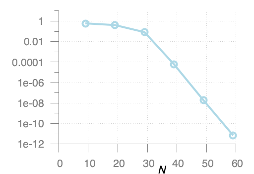
Figure 5.1. $L^{2}$ error in log scale.

Number of	Discrete $L^{2}$	Order of
modes $N$	error $\mathcal{E}(N)$	accuracy
$10$	$6.0072\,\times\,10^{-01}$	X
$20$	$4.0877\,\times\,10^{-01}$	0.5
$30$	$8.3406\,\times\,10^{-02}$	3.9
$40$	$6.0200\,\times\,10^{-05}$	25
$50$	$1.8176\,\times\,10^{-07}$	36
$60$	$7.0635\,\times\,10^{-12}$	43

Table 5.1. $L^{2}$ error with respect to the number of Hermite modes $N$.

6. Conclusion

In conclusion, we have introduced a new approach to discretize the von Neumann equation in the semi-classical limit. By using Weyl’s variables and a truncated Hermite expansion of the density operator, we are able to address the stiffness due to the semi-classical scaling of the equation. Our method allows for error estimates by leveraging the propagation of regularity on the exact solution. Therefore, we believe that our asymptotic preserving numerical approximation, coupled with Hermite polynomials, represents an interesting approach for accurately solving the von Neumann equation in the semi-classical regime.

Appendix A Proof of Proposition 4.1

The case $m=0$ corresponds to the conservation of the $L^{2}$ norm

$$\|R(t)\|_{L^{2}}\,=\,\|R^{in}\|_{L^{2}}\,,\qquad t\geq 0.$$

Let us begin with the propagation of quantities corresponding to phase-space derivatives in the Wigner equation, that is to say $\partial_{x}R$ and $yR$. Later, it will be convenient to use the notation

$$L\,=\,\max(1,\|V^{\prime\prime}\|_{L^{\infty}})\,.$$

On the one hand, the equation for derivative of $R$ is given by

$$\partial_{t}\partial_{x}R(t|\,x,y) = i\,\partial_{x}\partial_{y}\partial_{x}R(t|\,x,y)\,-\,i\,\partial_{x}\left(\frac{V(x+\frac{1}{2}\hbar y)-V(x-\frac{1}{2}\hbar y)}{\hbar}R(t|\,x,y)\right)$$

$$= i\,\partial_{x}\partial_{y}\partial_{x}R(t|\,x,y)\,-\,i\,\frac{V(x+\frac{1}{2}\hbar y)-V(x-\frac{1}{2}\hbar y)}{\hbar}\partial_{x}R(t|\,x,y)$$

$$- \,i\,\frac{V^{\prime}(x+\frac{1}{2}\hbar y)\,-\,V^{\prime}(x-\frac{1}{2}\hbar y)}{\hbar}R(t|\,x,y)\,,$$

so that

$$\partial_{x}R(t|\,x,y)\,=\,\mathcal{S}_{\hbar}(t)\partial_{x}R(0|x,y)\,-\,i\,\int_{0}^{t}\mathcal{S}_{\hbar}(t-s)\frac{V^{\prime}(x+\frac{1}{2}\hbar y)-V^{\prime}(x-\frac{1}{2}\hbar y)}{\hbar}\,R(s|\,x,y)\,\mathrm{d}s\,,$$

where $\mathcal{S}_{\hbar}(t)$ represents the (semi)group (1.7) associated to (1.4). Hence since $\mathcal{S}_{\hbar}(t)$ is an isometry.

$$\|\partial_{x}R(t)\|_{L^{2}} \leq \|\partial_{x}R(0)\|_{L^{2}}\,+\,\int_{0}^{t}\left\|\frac{V^{\prime}(x+\frac{1}{2}\hbar y)-V^{\prime}(x-\frac{1}{2}\hbar y)}{\hbar\,y}\,y\,R(s|\,x,y)\right\|_{L^{2}}\,\mathrm{d}s$$

$$\leq \|\partial_{x}R(0)\|_{L^{2}}+\|V^{\prime\prime}\|_{L^{\infty}}\,\int_{0}^{t}\|y\,R(s)\|_{L^{2}}\mathrm{d}s\,.$$

Similarly, we have

$$\partial_{t}\left(y\,R(t|\,x,y)\right) = i\,\partial_{x}\partial_{y}\left(y\,R(t|\,x,y)\right)\,-\,i\,\frac{V(x+\frac{1}{2}\hbar y)-V(x-\frac{1}{2}\hbar y)}{\hbar}\left(y\,R(t|\,x,y)\right)$$

$$- i\,\partial_{x}R(t|\,x,y)\,,$$

so that, arguing as above, we have

$$\|y\,R(t)\|_{L^{2}}\leq\|y\,R(0)\|_{L^{2}}\,+\,\int_{0}^{t}\|\partial_{x}R(s)\|_{L^{2}}\mathrm{d}s\,.$$

Summarizing, we have proved that

$$\|\partial_{x}R(t)\|_{L^{2}} + \|y\,R(t)\|_{L^{2}}-\|\partial_{x}R(0)\|_{L^{2}}\,-\,\|y\,R(0)\|_{L^{2}}$$

$$\leq \int_{0}^{t}\left(\|V^{\prime\prime}\|_{L^{\infty}}\,\|y\,R(s)\|_{L^{2}}\,+\,\|\partial_{x}R(s)\|_{L^{2}}\right)\mathrm{d}s$$

$$\leq L\,\int_{0}^{t}\left(\|\partial_{x}R(s)\|_{L^{2}}\,+\,\|y\,R(s)\|_{L^{2}}\right)\mathrm{d}s\,,$$

hence by applying Gronwall’s lemma, we have

(A.1) $$\|\partial_{x}R(t)\|_{L^{2}}\,+\,\|y\,R(t)\|_{L^{2}}\,\leq\,\left(\|\partial_{x}R(0)\|_{L^{2}}\,+\,\|y\,R(0)\|_{L^{2}}\right)\,e^{L\,t}\,.$$

Here we observe that this estimate is uniform in (in fact independent of) $\hbar$. Next we discuss the propagation of quantities corresponding to moments in the Wigner equation, that is, $xR$ and $\partial_{y}R$. On the one hand, the equation for $xR(t|\,x,y)$ is

$$\partial_{t}(xR(t|\,x,y)) = i\,\partial_{x}\partial_{y}(xR(t|\,x,y))\,-\,i\,\frac{V(x+\frac{1}{2}\hbar y)-V(x-\frac{1}{2}\hbar y)}{\hbar}(xR(t|\,x,y))$$

$$- \,i\,\partial_{y}R(t|\,x,y)\,,$$

so that, arguing as above

$$\|x\,R(t)\|_{L^{2}}\,\leq\,\|x\,R(0)\|_{L^{2}}\,+\,\int_{0}^{t}\|\partial_{y}R(s)\|_{L^{2}}\mathrm{d}s\,.$$

On the other hand, the equation for $\partial_{y}R$ is

$$\partial_{t}\partial_{y}R(t|\,x,y) = i\,\partial_{x}\partial_{y}\partial_{y}R(t|\,x,y)\,-\,i\,\partial_{y}\left(\frac{V(x+\frac{1}{2}\hbar y)-V(x-\frac{1}{2}\hbar y)}{\hbar}\,R(t|\,x,y)\right)$$

$$= i\,\partial_{x}\partial_{y}\partial_{y}R(t|\,x,y)\,-\,i\frac{V(x+\frac{1}{2}\hbar y)-V(x-\frac{1}{2}\hbar y)}{\hbar}\,\partial_{y}R(t|\,x,y)$$

$$- \frac{i}{2}\,\left(V^{\prime}\left(x+\frac{1}{2}\hbar y\right)+V^{\prime}\left(x-\frac{1}{2}\hbar y\right)\right)\,R(t|\,x,y)\,.$$

Here it is worth mentioning that there are several options for the treatment of the last term on the last right-hand side. One could of course assume that $V^{\prime}$ is bounded, but this is not very satisfying as it leaves out the case of a harmonic oscillator, where $V$ is quadratic in $x$. In the latter case, one can assume instead that $V^{\prime\prime}$ is bounded. This is the simpler case, allowing us to include a confining quadratic potential if needed. Besides, since $V(x)\to+\infty$ as $|x|\to+\infty$, it has a minimum point at $x_{0}\in\mathbb{R}$. Without loss of generality, assume henceforth that $x_{0}=0$, so that $V^{\prime}(0)=0$. Therefore, by the mean value inequality

$$|V^{\prime}(z)-V^{\prime}(0)|\,\leq\,\|V^{\prime\prime}\|_{L^{\infty}}\,|z|\,,$$

and hence, having recast the last equality as

$$\partial_{t}\partial_{y}R(t|\,x,y) = i\,\partial_{x}\partial_{y}\partial_{y}R(t|\,x,y)\,-\,i\frac{V(x+\frac{1}{2}\hbar y)\,-\,V(x-\frac{1}{2}\hbar y)}{\hbar}\,\partial_{y}R(t|\,x,y)$$

$$- \,i\,V^{\prime}(x)R(t|\,x,y)\,-\,i\,\frac{V^{\prime}(x+\tfrac{1}{2}\hbar y)\,+\,V^{\prime}(x-\tfrac{1}{2}\hbar y)\,-\,2\,V^{\prime}(x)}{2}\,R(t|\,x,y)\,,$$

we conclude as above that

$$\|\partial_{y}R(t)\|_{L^{2}}\,\leq\,\|\partial_{y}R(0)\|_{L^{2}}\,+\,\|V^{\prime\prime}\|_{L^{\infty}}\,\int_{0}^{t}\left(\|x\,R(s)\|_{L^{2}}\,+\,\frac{\hbar}{2}\,\|y\,R(s)\|_{L^{2}}\right)\,\mathrm{d}s\,.$$

Combining this inequality with the one for $xR(t|\,x,y)$ leads to

$$\|x\,R(t)\|_{L^{2}}\,+\,\|\partial_{y}R(t)\|_{L^{2}}\,-\,\|x\,R(0)\|_{L^{2}}\,-\,\|\partial_{y}R(0)\|_{L^{2}}$$

$$\leq\,\int_{0}^{t}\left(\|V^{\prime\prime}\|_{L^{\infty}}\|x\,R(s)\|_{L^{2}}\,+\,\|\partial_{y}R(s)\|_{L^{2}}\right)\,\mathrm{d}s\,+\,\frac{\hbar}{2}\,\|V^{\prime\prime}\|_{L^{\infty}}\,\int_{0}^{t}\|y\,R(s)\|_{L^{2}}\,\mathrm{d}s\,.$$

The last term on the right-hand side is bounded as in (A.1), by

$$\left(\|\partial_{x}R(0)\|_{L^{2}}+\|y\,R(0)\|_{L^{2}}\right)\,e^{t\max(1,\|V^{\prime\prime}\|_{L^{\infty}})}\,.$$

Thus

$$\|x\,R(t)\|_{L^{2}}\,+\;\|\partial_{y}R(t)\|_{L^{2}}\,-\,\|x\,R(0)\|_{L^{2}}\,-\,\|\partial_{y}R(0)\|_{L^{2}}$$

$$\leq L\int_{0}^{t}(\|x\,R(s\|_{L^{2}}\,+\,\|\partial_{y}R(s)\|_{L^{2}})\,\mathrm{d}s\,+\,\frac{\hbar}{2}\,\left(\|\partial_{x}R(0)\|_{L^{2}}\,+\,\|y\,R(0)\|_{L^{2}}\right)\,(e^{Lt}-1)$$

and by Gonwall’s lemma, we conclude that

(A.2) $$\|x\,R(t)\|_{L^{2}}\,+\,\|\partial_{y}R(t)\|_{L^{2}} \leq\left(\|x\,R(0)\|_{L^{2}}\,+\,\|\partial_{y}R(0)\|_{L^{2}}\right)\,e^{Lt}$$

$$+\,\frac{\hbar}{2}\,\left(\|\partial_{x}R(0)\|_{L^{2}}+\|y\,R(0)\|_{L^{2}}\right)\,(e^{Lt}-1)\,e^{Lt}\,.$$

Unlike (A.1), this bound is not independent of $\hbar$, but its $\hbar$-dependence is not singular as $\hbar\to 0$. Together with (A.1), the inequality (A.2) is easily transformed into a uniform in $\hbar$ bound for $\hbar\in(0,2]$, say:

(A.3) $$\mathcal{N}_{1}(t) \leq\,\mathcal{N}_{1}(0)\,e^{Lt}\,+\,\frac{\hbar}{2}\,\left(\|\partial_{x}R(0)\|_{L^{2}}+\|y\,R(0)\|_{L^{2}}\right)\,(e^{Lt}-1)\,e^{Lt}$$

$$\leq\,\mathcal{N}_{1}(0)\,e^{Lt}\,+\,\frac{\hbar}{2}\,\mathcal{N}_{1}(0)\,(e^{Lt}-1)\,e^{Lt}$$

$$\leq\,\mathcal{N}_{1}(0)\,e^{2Lt}\,.$$

Thus it yields the result for $n=1$.

We now proceed in the same way, for each integer $a$, $b$, $\alpha$ and $\beta$ such that $a+b+\alpha+\beta=n$ and seek an equation for

$$x^{a}\partial_{x}^{b}y^{\alpha}\partial_{y}^{\beta}R(t|\,x,y).$$

Starting from

$$\partial_{t}R(t|\,x,y)\,=\,i\,\partial_{x}\partial_{y}R(t|\,x,y)\,-\,i\,\frac{V(x+\frac{1}{2}\hbar y)-V(x-\frac{1}{2}\hbar y)}{\hbar}\,R(t|\,x,y)\,,$$

we see that

$$\partial_{t}\left(x^{a}\partial_{x}^{b}y^{\alpha}\partial_{y}^{\beta}R(t|\,x,y)\right) \,=\,i\,\partial_{x}\partial_{y}\left(x^{a}\partial_{x}^{b}y^{\alpha}\partial_{y}^{\beta}R(t|\,x,y)\right)$$

$$\,-\,i\,\frac{V(x+\frac{1}{2}\hbar y)-V(x-\frac{1}{2}\hbar y)}{\hbar}\,\left(x^{a}\partial_{x}^{b}y^{\alpha}\partial_{y}^{\beta}R(t|\,x,y)\right)\,+\,i\,\mathcal{T}_{1}\,-\,i\,\mathcal{T}_{2}\,,$$

where

$$\left\{\begin{array}[]{l}\displaystyle\mathcal{T}_{1}\,=\,\left[x^{a}\partial_{x}^{b}y^{\alpha}\partial_{y}^{\beta},\,\partial_{x}\partial_{y}\right]\,R(t|\,x,y)\,,\\[8.99994pt] \displaystyle\mathcal{T}_{2}\,=\,\left[x^{a}\partial_{x}^{b}y^{\alpha}\partial_{y}^{\beta},\frac{V(x+\frac{1}{2}\hbar y)-V(x-\frac{1}{2}\hbar y)}{\hbar}\right]\,R(t|\,x,y)\,.\end{array}\right.$$

Hence, the idea is to treat $\mathcal{T}_{j}$ as source terms for $j=1,2$, to find

$$\|x^{a}\partial_{x}^{b}y^{\alpha}\partial_{y}^{\beta}R(t|\,x,y)\|_{L^{2}}\,\leq \|x^{a}\partial_{x}^{b}y^{\alpha}\partial_{y}^{\beta}R(0|x,y)\|_{L^{2}}$$

$$\,+\,\int_{0}^{t}(\|\mathcal{T}_{1}(s|\,\cdot,\cdot)\|_{L^{2}}\,+\,\|\mathcal{T}_{2}(s|\,\cdot,\cdot)\|_{L^{2}})\mathrm{d}s\,.$$

First, we consider $\mathcal{T}_{1}$ and use that

$$\left[x^{a}\partial_{x}^{b}y^{\alpha}\partial_{y}^{\beta},\partial_{x}\partial_{y}\right] =\,\left[x^{a}\partial_{x}^{b}y^{\alpha}\partial_{y}^{\beta},\partial_{x}\right]\,\partial_{y}\,+\,\partial_{x}\left[x^{a}\partial_{x}^{b}y^{\alpha}\partial_{y}^{\beta},\partial_{y}\right]\,,$$

$$\,=\,\left[x^{a},\,\partial_{x}\right]\,\partial_{x}^{b}y^{\alpha}\partial_{y}^{\beta}\partial_{y}\,+\,\partial_{x}x^{a}\partial_{x}^{b}\,\left[y^{\alpha},\partial_{y}\right]\,\partial_{y}^{\beta}$$

$$\,=\,-ax^{a-1}\,\partial_{x}^{b}y^{\alpha}\partial_{y}^{\beta+1}\,-\,\alpha\,\partial_{x}x^{a}\partial_{x}^{b}y^{\alpha-1}\partial_{y}^{\beta}$$

$$\,=\,-a\,x^{a-1}\,\partial_{x}^{b}y^{\alpha}\partial_{y}^{\beta+1}\,-\,\alpha x^{a}\partial_{x}^{b+1}y^{\alpha-1}\partial_{y}^{\beta}\,-\,\alpha\,\left[\partial_{x},x^{a}\right]\partial_{x}^{b}y^{\alpha-1}\partial_{y}^{\beta}$$

$$\,=\,-a\,x^{a-1}\partial_{x}^{b}y^{\alpha}\partial_{y}^{\beta+1}\,-\,\alpha x^{a}\partial_{x}^{b+1}y^{\alpha-1}\partial_{y}^{\beta}\,-\,\alpha\,a\,x^{a-1}\,\partial_{x}^{b}y^{\alpha-1}\partial_{y}^{\beta}\,.$$

In the first two terms on the right-hand side, the sum of exponents is

$$a-1+b+\alpha+\beta+1=a+b+1+\alpha-1+\beta=n\,,$$

equal to that in $x^{a}\partial_{x}^{b}y^{\alpha}\partial_{y}^{\beta}$, whereas the last term has a sum of exponents

$$a-1+b+\alpha-1+\beta=n-2$$

less than that in $x^{a}\partial_{x}^{b}y^{\alpha}\partial_{y}^{\beta}$. Hence we obtain

$$\|\mathcal{T}_{1}(s|\cdot,\cdot)\|_{L^{2}}\,\leq\,2\,n\,\mathcal{N}_{n}(s)\,+\,n^{2}\mathcal{N}_{n-2}(s)\,\leq\,(2n+n^{2})\,\mathcal{N}_{n}(s)\,.$$

Now for the second term $\mathcal{T}_{2}$, we have

$${}\left[x^{a}\partial_{x}^{b}y^{\alpha}\partial_{y}^{\beta},\frac{V(x+\frac{\hbar}{2}y)-V(x-\frac{\hbar}{2}y)}{\hbar}\right] =\,x^{a}\left[\partial_{x}^{b},\frac{V(x+\frac{\hbar}{2}y)-V(x-\frac{\hbar}{2}y)}{\hbar}\right]y^{\alpha}\partial_{y}^{\beta}$$

$$+\,x^{a}\partial_{x}^{b}y^{\alpha}\left[\partial_{y}^{\beta},\frac{V(x+\frac{\hbar}{2}y)-V(x-\frac{\hbar}{2}y)}{\hbar}\right]\,.$$

By Leibniz’s formula

$$\left[\partial_{x}^{b},\frac{V(x+\frac{\hbar}{2}y)-V(x-\frac{\hbar}{2}y)}{\hbar}\right]\,= \sum_{j=1}^{b}{b\choose j}\,\frac{V^{(j)}(x+\frac{\hbar}{2}y)-V^{(j)}(x-\frac{\hbar}{2}y)}{\hbar}\,\partial_{x}^{b-j}\,,$$

$$\left[\partial_{y}^{\beta},\frac{V(x+\frac{\hbar}{2}y)-V(x-\frac{\hbar}{2}y)}{\hbar}\right]\,= \sum_{k=1}^{\beta}{\beta\choose k}\,\frac{V^{(k)}(x+\frac{\hbar}{2}y)-(-1)^{k}\,V^{(k)}(x-\frac{\hbar}{2}y)}{2^{k}\,\hbar}\,\hbar^{k}\,\partial_{y}^{\beta-k}\,,$$

so that

$$\left[x^{a}\partial_{x}^{b}y^{\alpha}\partial_{y}^{\beta},\frac{V(x+\frac{\hbar}{2}y)-V(x-\frac{\hbar}{2}y)}{\hbar}\right]$$

$$\quad\,=\,\sum_{j=1}^{b}{b\choose j}\frac{V^{(j)}(x+\frac{\hbar}{2}y)-V^{(j)}(x-\frac{\hbar}{2}y)}{\hbar}x^{a}\partial_{x}^{b-j}y^{\alpha}\partial_{y}^{\beta}$$

$$\quad\quad\,+\,\sum_{k=1}^{\beta}{\beta\choose k}\frac{V^{(k)}(x+\frac{\hbar}{2}y)-(-1)^{k}\,V^{(k)}(x-\frac{\hbar}{2}y)}{2^{k}\hbar}\hbar^{k}x^{a}\partial_{x}^{b}y^{\alpha}\partial_{y}^{\beta-k}$$

$$\quad\quad\,+\,\sum_{k=1}^{\beta}{\beta\choose k}x^{a}\left[\partial^{b}_{x},\frac{V^{(k)}(x+\frac{\hbar}{2}y)-(-1)^{k}\,V^{(k)}(x-\frac{\hbar}{2}y)}{2^{k}\hbar}\right]\hbar^{k}y^{\alpha}\partial_{y}^{\beta-k}$$

$$\quad\,=\,b\,\frac{V^{\prime}(x+\frac{\hbar}{2}y)-V^{\prime}(x-\frac{\hbar}{2}y)}{\hbar y}\,x^{a}\partial_{x}^{b-1}y^{\alpha+1}\partial_{y}^{\beta}$$

$$\quad\quad\,+\,\sum_{j=2}^{b}{b\choose j}\,\frac{V^{(j)}(x+\frac{\hbar}{2}y)-V^{(j)}(x-\frac{\hbar}{2}y)}{\hbar y}\,x^{a}\,\partial_{x}^{b-j}y^{\alpha+1}\partial_{y}^{\beta}$$

$$\quad\quad\,+\,\beta\,\frac{V^{\prime}(x+\frac{\hbar}{2}y)+V^{\prime}(x-\frac{\hbar}{2}y)-2\,V^{\prime}(x)}{2\hbar y}\,\hbar\,x^{a}\,\partial_{x}^{b}y^{\alpha+1}\partial_{y}^{\beta-1}$$

$$\quad\quad\,+\,\beta\,\frac{V^{\prime}(x)-V^{\prime}(0)}{x}\,x^{a+1}\,\partial_{x}^{b}y^{\alpha}\partial_{y}^{\beta-1}\,+\,\beta\,V^{\prime}(0)\,x^{a}\,\partial_{x}^{b}y^{\alpha}\partial_{y}^{\beta-1}$$

$$\quad\quad\,+\,\sum_{k=2}^{\beta}{\beta\choose k}\,\frac{V^{(k)}(x+\frac{\hbar}{2}y)-(-1)^{k}\,V^{(k)}(x-\frac{\hbar}{2}y)}{2^{k}\hbar}\,\hbar^{k}\,x^{a}\,\partial_{x}^{b}y^{\alpha}\partial_{y}^{\beta-k}$$

$$\quad\quad\,+\,\sum_{k=1}^{\beta}\sum_{j=1}^{b}{\beta\choose k}{b\choose j}\,\frac{V^{(k+j)}(x+\frac{\hbar}{2}y)-(-1)^{k}\,V^{(k+j)}(x-\frac{\hbar}{2}y)}{2^{k}\hbar}\,\hbar^{k}\,x^{a}\,\partial^{b-j}_{x}y^{\alpha}\partial_{y}^{\beta-k}\,.$$

The first term in the right-hand side involves the ratio

$$\left|\,\frac{V^{\prime}(x+\frac{\hbar}{2}y)\,-\,V^{\prime}(x-\frac{\hbar}{2}y)}{\hbar\;y}\right|\,\leq\|V^{\prime\prime}\|_{L^{\infty}}\,,$$

and the monomial $x^{a}\partial_{x}^{b-1}y^{\alpha+1}\partial_{y}^{\beta}$, whose exponents add up to

$$a+b-1+\alpha+1+\beta=n\,,$$

which is equal to the sum of exponents in the monomial $x^{a}\partial_{x}^{b}y^{\alpha}\partial_{y}^{\beta}$. The second term in the right-hand side involves monomials whose exponents add up to

$$a+b-j+\alpha+1+\beta\,<\,n$$

since $j\geq 2$, multiplied by the ratio

$$\left|\,\frac{V^{(j)}(x+\frac{\hbar}{2}y)\,-\,V^{(j)}(x-\frac{\hbar}{2}y)}{\hbar\,y}\right|\,\leq\|V^{(j+1)}\|_{L^{\infty}}<\infty\,.$$

The last three terms on the right-hand side involve monomials whose exponents add up to

$$a+b-j+\alpha+\beta-k\,\leq\,n$$

since $j+k\geq 1$, multiplied by $V^{\prime}(0)$ or a ratio of the form

$$\left|\,\frac{V^{(k+j)}(x+\frac{\hbar}{2}y)-(-1)^{k}\,V^{(k+j)}(x-\frac{\hbar}{2}y)}{2^{k}\hbar}\right|\,\hbar^{k}\,\leq\,\|V^{(k+j)}\|_{L^{\infty}}\,\hbar^{k-1}$$

since $k\geq 1$ and $k+j\geq 2$. There remains the third and fourth terms, involving monomials whose exponents add up to $a+b+\alpha+\beta$, multiplied by ratios of the form

$$\left|\,\frac{V^{\prime}(x+\frac{\hbar}{2}y)\,+\,V^{\prime}(x-\frac{\hbar}{2}y)-2\,V^{\prime}(x)}{2\hbar\,y}\right|\,\leq\,\frac{1}{2}\|V^{\prime\prime}\|_{L^{\infty}}\,<\,\infty\,,$$

or

$$\left|\,\frac{V^{\prime}(x)-V^{\prime}(0)}{x}\right|\,\leq\|V^{\prime\prime}\|_{L^{\infty}}<\infty\,.$$

Summarizing, assuming that $\hbar\leq 1$

$$\|\mathcal{T}_{2}(s|\,\cdot,\cdot)\|_{L^{2}} \leq\,n\,\|V^{\prime\prime}\|_{L^{\infty}}\,\mathcal{N}_{n}(s)\,+\,\underbrace{\sum_{j=2}^{b}{b\choose j}\|V^{(j+1)}\|_{L^{\infty}}\,\mathcal{N}_{n-j+1}(s)}_{\leq 2^{n}\max_{2\leq i\leq n}\|V^{(i+1)}\|_{L^{\infty}}\mathcal{N}_{n-1}(s)}\,+\,\frac{1}{2}\,\|V^{\prime\prime}\|_{L^{\infty}}\,n\,\hbar\,\mathcal{N}_{n}(s)$$

$$\quad\,+\,\|V^{\prime\prime}\|_{L^{\infty}}\,n\,\mathcal{N}_{n}(s)\,+\,n\,|V^{\prime}(0)|\,\mathcal{N}_{n-1}(s)\,+\,\underbrace{\sum_{k=2}^{\beta}{\beta\choose k}\|V^{(k)}\|_{L^{\infty}}\,\hbar^{k-1}\,\mathcal{N}_{n-k}(s)}_{\leq\,2^{n}\,\max_{2\leq i\leq n}\|V^{(i)}\|_{L^{\infty}}\,\mathcal{N}_{n-2}(s)}$$

$$\quad\,+\,\underbrace{\sum_{k=1}^{\beta}\sum_{j=1}^{b}{\beta\choose k}{b\choose j}\|V^{(k+j)}\|_{L^{\infty}}\,\hbar^{k-1}\,\mathcal{N}_{n-k-j}(s)}_{\leq\,2^{n}\cdot 2^{n}\,\max_{2\leq i\leq n}\|V^{(i)}\|_{L^{\infty}}\mathcal{N}_{n-2}(s)}\,.$$

Hence, it yields

$$\|\mathcal{T}_{2}(s|\cdot,\cdot)\|_{L^{2}} \leq\,\max\left(|V^{\prime}(0),\,\max_{2\leq k\leq{\color[rgb]{1,0,0}n+1}}\|V^{(k)}\|_{L^{\infty}}\right)\,\left(n+2^{n}+\frac{1}{2}\,n\,\hbar+n+n+2^{n}+2^{n}\cdot 2^{n}\right)\,\mathcal{N}_{n}(s)$$

$$\leq\,\max\left(|V^{\prime}(0),\,\max_{2\leq k\leq n+1}\|V^{(k)}\|_{L^{\infty}}\right)\left(\frac{7}{2}+2^{n}\right)\,(2^{n}+2)\,\mathcal{N}_{n}(s)\,.$$

Thus, we have proved that

$$\|x^{a}\partial_{x}^{b}y^{\alpha}\partial_{y}^{\beta}R(t)\|_{L^{2}}\,\leq\,\|x^{a}\partial_{x}^{b}y^{\alpha}\partial_{y}^{\beta}R(0)\|_{L^{2}}$$

$$+\,\left(1+\max\left(|V^{\prime}(0),\max_{2\leq k\leq n+1}\|V^{(k)}\|_{L^{\infty}}\right)\right)\,\int_{0}^{t}\left(\frac{7}{2}\,+\,2^{n}\right)\,(2^{n}+2)\,\mathcal{N}_{n}(s)\,\mathrm{d}s\,,$$

so that

$$\mathcal{N}_{n}(t)\,\leq\,\mathcal{N}_{n}(0)$$

$$+\left(1+\max\left(|V^{\prime}(0),\max_{2\leq k\leq n+1}\|V^{(k)}\|_{L^{\infty}}\right)\right)\,\left(\frac{7}{2}+2^{n}\right)\,(2^{n}+2)(n+1)^{4}\,\int_{0}^{t}\mathcal{N}_{n}(s)\mathrm{d}s$$

and one concludes by Gronwall’s inequality.

References

- [1] A. G. Athanassoulis. Smoothed Wigner transforms in the numerical simulation of semiclassical (high-frequency) wave propagation. Preprint, arXiv:0704.3404, 2007.
- [2] P. Bader, A. Iserles, K. Kropielnicka, and P. Singh. Effective approximation for the semiclassical Schrödinger equation. Foundations of Computational Mathematics, 14:689–720, 2014.
- [3] W. Bao, S. Jin, and P. A. Markowich. On time-splitting spectral approximations for the Schrödinger equation in the semiclassical regime. Journal of Computational Physics, 175(2):487–524, 2002.
- [4] C. Bardos, F. Golse, and D. Levermore. Fluid dynamic limits of kinetic equations. I. Formal derivations. J. Statist. Phys., 63(1-2):323–344, 1991.
- [5] M. Berman, R. Kosloff, and H. Tal-Ezer. Solution of the time-dependent Liouville-von Neumann equation: dissipative evolution. Journal of Physics A: Mathematical and General, 25(5):1283, 1992.
- [6] M. Bessemoulin-Chatard and F. Filbet. On the stability of conservative discontinuous Galerkin/Hermite spectral methods for the Vlasov-Poisson system. Journal of Computational Physics, 451:Paper No. 110881, 28, 2022.
- [7] M. Bessemoulin-Chatard and F. Filbet. On the convergence of discontinuous Galerkin/Hermite spectral methods for the Vlasov–Poisson system. SIAM Journal on Numerical Analysis, 61(4):1664–1688, 2023.
- [8] A. Blaustein. Structure preserving solver for Multi-dimensional Vlasov-Poisson type equations. preprint https://hal.science/hal-04440391v1, 2024.
- [9] A. Blaustein and F. Filbet. A structure and asymptotic preserving scheme for the Vlasov-Poisson-Fokker-Planck model. Journal of Computational Physics, 498:112693, 2024.
- [10] A. Blaustein and F. Filbet. On a discrete framework of hypocoercivity for kinetic equations. Mathematics of Computation, 93(345):163–202, 2024.
- [11] Y. Brenier. Convergence of the Vlasov-Poisson system to the incompressible Euler equations. Comm. Partial Differential Equations, 25(3-4):737–754, 2000.
- [12] H. Brézis. Analyse Fonctionnelle, Théorie et Applications. Masson, Paris, 1983, (English Translation) Functional Analysis, 2011.
- [13] D. Fang, S. Jin, and C. Sparber. An efficient time-splitting method for the Ehrenfest dynamics. Multiscale Modeling & Simulation, 16(2):900–921, 2018.
- [14] F. Filbet and F. Golse. On the approximation of the von-neumann equation in the semi-classical limit. part i: Numerical algorithm. Journal of Computational Physics, 527:113810, 2025.
- [15] F. Filbet and T. Xiong. Conservative discontinuous Galerkin/Hermite spectral method for the Vlasov-Poisson system. Communications on Applied Mathematics and Computation, 4(1):34–59, 2022.
- [16] F. Golse and M. Jakob. Velocity Averaging for the Mixed State Wigner Transform. preprint, 2024.
- [17] F. Golse, S. Jin, and T. Paul. On the convergence of time splitting methods for quantum dynamics in the semiclassical regime. Foundations of Computational Mathematics, 21(3):613–647, 2021.
- [18] B. Hellsing and H. Metiu. An efficient method for solving the quantum Liouville equation: Applications to electronic absorption spectroscopy. Chemical physics letters, 127(1):45–49, 1986.
- [19] M. Hochbruck and C. Lubich. Exponential integrators for quantum-classical molecular dynamics. BIT Numerical Mathematics, 39:620–645, 1999.
- [20] J. P. Holloway. Spectral velocity discretizations for the Vlasov-Maxwell equations. Transport Theory and Statistical Physics, 25(1):1–32, 1996.
- [21] S. Jin. Asymptotic-preserving schemes for multiscale physical problems. Acta Numerica, 31:415–489, 2022.
- [22] S. Jin, P. Markowich, and C. Sparber. Mathematical and computational methods for semiclassical Schrödinger equations. Acta Numerica, 20:121–209, 2011.
- [23] P. D. Lax. The scope of the energy method. Bull. Amer. Math. Soc., 66:32–35, 1960.
- [24] P. D. Lax and R. D. Richtmyer. Survey of the stability of linear finite difference equations. Comm. Pure Appl. Math., 9:267–293, 1956.
- [25] N. Lerner. Metrics on the phase space and non-self adjoint pseudo-differential operators, volume 3. Springer Science & Business Media, 2011.
- [26] P.-L. Lions and T. Paul. Sur les mesures de Wigner. Revista matemática iberoamericana, 9(3):553–618, 1993.
- [27] P. A. Markowich and H. Neunzert. On the equivalence of the Schrödinger and the quantum Liouville equations. Mathematical Methods in the Applied Sciences, 11(4):459–469, 1989.
- [28] P. A. Markowich, P. Pietra, and C. Pohl. Numerical approximation of quadratic observables of Schrödinger-type equations in the semi-classical limit. Numerische Mathematik, 81:595–630, 1999.
- [29] P. A. Markowich and C. Ringhofer. An analysis of the quantum Liouville equation. ZAMM-Journal of Applied Mathematics and Mechanics/Zeitschrift für Angewandte Mathematik und Mechanik, 69(3):121–127, 1989.
- [30] P. A. Markowich, C. A. Ringhofer, and C. Schmeiser. Semiconductor equations. Springer Science & Business Media, 2012.
- [31] B. Miao, G. Russo, and Z. Zhou. A novel spectral method for the semiclassical Schrödinger equation based on the Gaussian wave-packet transform. IMA Journal of Numerical Analysis, 43(2):1221–1261, 2023.
- [32] G. Russo and P. Smereka. The Gaussian wave packet transform: Efficient computation of the semi-classical limit of the Schrödinger equation. Part 1–Formulation and the one dimensional case. Journal of Computational Physics, 233:192–209, 2013.
- [33] G. Russo and P. Smereka. The Gaussian wave packet transform: efficient computation of the semi-classical limit of the Schrödinger equation. Part 2. Multidimensional case. Journal of Computational Physics, 257:1022–1038, 2014.
- [34] J. W. Schumer and J. P. Holloway. Vlasov simulations using velocity-scaled Hermite representations. Journal of Computational Physics, 144(2):626–661, 1998.
- [35] J. Sellier, M. Nedjalkov, I. Dimov, and S. Selberherr. A comparison of approaches for the solution of the Wigner equation. Mathematics and Computers in Simulation, 107:108–119, 2015.
- [36] D. Sels, F. Brosens, and W. Magnus. Wigner distribution functions for complex dynamical systems: A path integral approach. Physica A: Statistical Mechanics and its Applications, 392(2):326–335, 2013.
- [37] S. Shao, T. Lu, and W. Cai. Adaptive conservative cell average spectral element methods for transient Wigner equation in quantum transport. Communications in Computational Physics, 9(3):711–739, 2011.
- [38] M. L. Van de Put, B. Sorée, and W. Magnus. Efficient solution of the Wigner-Liouville equation using a spectral decomposition of the force field. Journal of Computational Physics, 350:314–325, 2017.
- [39] Y. Xie and Z. Zhou. Frozen Gaussian sampling: a mesh-free Monte Carlo method for approximating semiclassical Schrödinger equations. Communications in Mathematical Sciences, 22(4):1133–1166, 2024.
- [40] Y. Xiong, Z. Chen, and S. Shao. An advective-spectral-mixed method for time-dependent many-body Wigner simulations. SIAM Journal on Scientific Computing, 38(4):B491–B520, 2016.