Acoustic turbulence: from the Zakharov-Sagdeev spectra to the Kadomtsev-Petviashvili spectrum

Abstract

This paper presents a brief review on theoretical and numerical works on three-dimensional acoustic turbulence both in a weakly nonlinear regime, when the amplitudes of sound waves are small, and in the case of strong nonlinearity. This review is based on the classical studies on weak acoustic turbulence by V.E. Zakharov (1965) and V.E. Zakharov and R.Z. Sagdeev (1970), on the one hand, and on the other hand, by B.B. Kadomtsev and V.I. Petviashvili (1972). Until recently, there were no convincing numerical experiments confirming one or the other point of view. In the works of the authors of this review in 2022 and 2024, strong arguments were found based on direct numerical modeling in favor of both theories. It is shown that the Zakharov-Sagdeev spectrum of weak turbulence $\propto k^{-3/2}$ is realized not only for small positive dispersion of sound waves, but also in the case of complete absence of dispersion. The calculated turbulence spectra in the weakly nonlinear regime have anisotropic distribution: for small $k$, narrow cones (jets) are formed, broadening in the Fourier space. For weak dispersion, the jets are smoothed out, and the turbulence spectrum tends to be isotropic in the region of short wavelengths. In the absence of dispersion, the turbulence spectrum is a discrete set of jets subjected to diffraction divergence. For each individual jet, nonlinear effects are much weaker than diffraction ones, which prevents the formation of shock waves. Thus, the weakly turbulent Zakharov-Sagdeev spectrum is realized due to the smallness of nonlinear effects compared to dispersion or diffraction. As the pumping level increases in the non-dispersive regime, when nonlinear effects begin to dominate, shock waves are formed. As a result, acoustic turbulence passes into a strongly nonlinear state in the form of an ensemble of random shocks described by the Kadomtsev-Petviashvili spectrum $\propto k^{-2}$.

Introduction

As is known, developed hydrodynamic turbulence at large Reynolds numbers, $Re\gg 1$, in the inertial interval is an example of a system with strong nonlinearity, when its energy coincides with the interaction Hamiltonian. Another classic example is acoustic turbulence, which exhibits both strong and weak regimes depending on the ratio of nonlinearity and linear wave characteristics. In this sense, acoustic turbulence is much more diverse and richer than hydrodynamic turbulence. When the nonlinear interaction of waves is small compared to linear effects, a weak turbulence regime [1] is realized, which can be studied on the basis of perturbation theory using the random phase approximation. The theory of weak turbulence [1, 2] statistically describes ensembles of interacting waves within the framework of the corresponding kinetic equations [1, 2]. This theory assumes that each wave with its random phase propagates almost freely for a long time and very rarely undergoes small deformations due to nonlinear interaction with other waves. To date, the theory of weak turbulence has found many applications, ranging from ocean and plasma waves, waves in solid state physics, in Bose-Einstein condensates and ending with turbulence in both astrophysics and high-energy physics. Here we will cite only some of the latest works on this topic: [3, 4, 5, 6, 7, 8, 9, 10]. It should be noted that for waves on the surface of a liquid, both capillary and gravitational (dispersive waves), the theory of weak turbulence has been confirmed with very high accuracy [11]. However, for acoustic turbulence, a sufficiently complete understanding has not been yet. This is due to two different approaches to the study of acoustic turbulence. The first works on this topic were carried out by V.E. Zakharov in 1965 [12], and then in 1970 by V.E. Zakharov and R.Z. Sagdeev [13] based on the theory of weak turbulence. As a result, in the region of weak positive dispersion, a scale-invariant turbulence spectrum $E(k)\propto k^{-3/2}$ was found, called the Zakharov-Sagdeev spectrum. This spectrum was an exact solution in the long-wave limit of the stationary kinetic equation for waves, proportional to the square root of the energy flux $\epsilon$ into the region of short wavelengths. In 1972, B.B. Kadomtsev and V.I. Petviashvili [14] proposed their spectrum, which is now called the Kadomtsev-Petviashvili spectrum, which has a different dependence $E(k)\propto k^{-2}$. According to [14], acoustic turbulence was considered as an ensemble of random shock waves. Shock waves arise as a result of the breaking of sound waves of finite amplitude. The $k^{-2}$ dependence is due to density jumps. Until recently, there was not a single direct numerical experiment in which one or the other spectrum was observed. In this review, based on numerical experiments [15], [16], it will be shown what are the criteria for the emergence of the Zakharov-Sagdeev and Kadomtsev-Petviashvili spectra. In both cases, for small but finite amplitudes, the main nonlinear process is the three-wave interaction, which is resonant when the synchronism conditions are met

$$\omega(\mathbf{k})=\omega(\mathbf{k_{1}})+\omega(\mathbf{k_{2}}),\quad\mathbf{k}=\mathbf{k_{1}}+\mathbf{k_{2}}$$ (1)

where $\omega=\omega(\mathbf{k})$ is the dispersion law of linear waves. If $\omega(\mathbf{k})=kc_{s}$, where $c_{s}$ is the speed of sound, then these relations are obviously satisfied only for parallel wave vectors $\mathbf{k_{i}}$. Thus, a triplet of interacting waves forms a ray in $k$-space. Obviously, the transition to a coordinate system moving with the velocity $c_{s}$ along a separate ray makes this wave system strongly nonlinear. In one-dimensional gas dynamics, this nonlinearity leads to the breaking of acoustic waves in accordance with the famous Riemann solution. In the multidimensional case, the transition to a moving coordinate system with the velocity $c_{s}$ is possible only for one given ray; for all other rays propagating at certain angles, such a transition is not correct. A set of continuously distributed beams with close angles of wave propagation forms an acoustic beam, which, as is known, is subject to diffraction in the transverse direction. For any small but finite transverse beam width, the phenomenon of diffraction divergence will inevitably arise. This effect was first discussed in the original paper by Zakharov and Sagdeev [13]; at almost the same time, similar ideas were developed in the work of [17] (see also [18]). From these considerations it follows that the regime of weak turbulence for acoustic waves can be realized not only in the case of weak dispersion, but also in a dispersion-free situation due to the diffraction divergence of the wave beam.

It should be noted that the resonance conditions (1) are also satisfied for acoustic waves with weak positive dispersion, when

$$\omega=kc_{s}(1+a^{2}k^{2}),\quad(a^{2}k^{2}\ll 1),$$ (2)

where $a$ is the dispersion parameter, which has the dimension of length. In the weakly dispersive case, the interacting waves form cones with small angles $\sim(ak)^{2}$ instead of rays. In the case of small nonlinear effects compared to the dispersion of the waves, a weakly turbulent regime of the evolution of sound waves can be realized. For this case, the exact isotropic solution of the kinetic equation for three-dimensional weak acoustic turbulence, obtained in [12, 13], has the form

$$E(k)=C_{KZ}\left(\rho c_{s}\epsilon\right)^{1/2}k^{-3/2},$$ (3)

where $C_{KZ}$ is the dimensionless Kolmogorov-Zakharov constant, $\rho$ is the equilibrium gas density. The power-law dependence on $\epsilon$ in (3) with the exponent $1/2$ corresponds to the resonant three-wave interactions (1). In the long-wave limit, such a spectrum is local and does not depend on the dispersion parameter of waves $a$ [12, 13]. However, in two-dimensional geometry, the spectrum of weak acoustic turbulence explicitly contains a dependence on $a$ [3]: $E(k)=C(\epsilon ac_{s})^{1/2}/k$, where $C$ is a dimensionless constant. It should be noted that this dependence of the spectrum on $k$ was given in [19] without derivation. As for the one-dimensional case, the theory of weak sound turbulence turns out to be inapplicable, as was shown by Benney and Saffman [20].

The existence of the Zakharov-Sagdeev spectrum (3) in the inertial interval, as a Kolmogorov-type spectrum, was confirmed in a number of works [21, 22, 23] in numerical solution of the kinetic equation for waves in the presence of long-wave pumping and high-frequency attenuation. It is important to note that numerical study of weak sound turbulence within the framework of the kinetic equation for waves in the three-dimensional case was carried out only for isotropic distributions.

With an increase in energy pumping, when the effects of nonlinear interaction of waves become comparable with linear dispersion, various nonlinear coherent structures arise: solitons, collapses, shock waves, etc. (see, for example, [24] and [25]). In this case, the behavior of the system is determined by the interaction of coherent structures with an ensemble of incoherent chaotic waves.

In the non-dispersive case, when nonlinear effects prevail over diffraction, the breaking of acoustic waves leads to the formation of propagating density discontinuities, which are the shock waves. In this regime, according to Kadomtsev and Petviashvili [14], acoustic turbulence is an ensemble of randomly distributed shocks. In this case, the spectrum of acoustic turbulence has the form:

$$E(k)=\frac{2S_{d}c_{s}^{2}\langle\delta\rho^{2}\rangle}{\pi\rho}k^{-2},$$ (4)

where $S_{d}$ is the density of shock waves per unit length, $\langle\delta\rho^{2}\rangle$ is the mean square of density jumps at discontinuities (see, for example, [26]). Note that the exponent of the power spectrum (4) does not depend on the dimension of space. In the one-dimensional case, the expression (4) is nothing more than the spectrum of turbulence, first found by Burgers [27]. Thus, at the present time, there are two different approaches to the description of acoustic non-dispersive turbulence, predicting different spectra for the same phenomenon.

The main objective of this review is to answer the fundamental question about the reason for the different behavior of the acoustic turbulence spectra (3) and (4). The paper presents the results of direct numerical simulation of sound wave turbulence in three-dimensional geometry [15, 16], which indicate the possibility of realizing both the weak turbulence Zakharov-Sagdeev spectrum (3) and the spectrum of Kadomtsev-Petviashvili (4) for three-dimensional acoustic waves in the regime of strong sound turbulence. The transition between these regimes is determined by the level of nonlinearity of the system. In the works of authors [15, 16] in 2022 and 2024, compelling criteria were found in favor of both theories. It is shown that the Zakharov-Sagdeev weak turbulence spectrum $\propto k^{-3/2}$ is realized not only at small positive dispersion of sound waves, but also in the case of complete absence of dispersion. The calculated turbulence spectra in the weakly nonlinear regime have an anisotropic distribution: in the region of small $k$, narrow cones (jets) are formed, broadening with increasing $k$ in Fourier space. In the case of weak dispersion, the jets are smoothed out, and the spectrum of turbulence tends to be isotropic in the region of short wavelengths. In the absence of dispersion, the turbulence spectrum is a discrete set of jets subjected to diffraction divergence. It was found that for each individual jet, nonlinear effects are much weaker than diffraction ones, which prevents the formation of shock waves. Thus, the weak turbulence Zakharov-Sagdeev spectra are realized due to the smallness of nonlinear effects in comparison with dispersion or diffraction. With an increase in the pumping level in the dispersionless regime, when nonlinear effects begin to prevail, shock waves (density discontinuities propagating in space) are formed. In a result, acoustic turbulence passes into a strongly nonlinear state in the form of an ensemble of random shocks described by the Kadomtsev-Petviashvili spectrum $\propto k^{-2}$.

The plan of the article is as follows. In the second section, we will consider in detail weak turbulence of sound waves using the kinetic equation and indicate the criteria for its applicability. In the third section, following the works of Zakharov and Sagdeev [12, 13], we will show how the Zakharov-Sagdeev spectrum is analytically found based on the solution of the kinetic equation for waves. The next section presents the numerical modeling scheme and its parameters. The fourth section presents the results of direct numerical modeling in both weak and strong turbulence modes. In addition to the turbulence spectra and their distributions, results on the statistics of turbulent states are presented. For weak turbulence, the amplitude distribution is close to Gaussian, and in the case of strong turbulence, the probability density distribution has power tails, indicating intermittency caused by shock waves.

This work is based on the lecture of E.A. Kuznetsov [28] read at the school ”Nonlinear Waves - 2024”.

I Kinetic equation

In this review, following the works of Zakharov and Sagdeev [12, 13], we will describe three-dimensional acoustic turbulence within the framework of the nonlinear string equation, often called the Boussinesq equation. This equation is written for a scalar quantity $u(\mathbf{r},t)$, depending on three spatial coordinates $\mathbf{r}=\{x,y,z\}$ and time $t$:

$$u_{tt}=\Delta u-2a^{2}\Delta^{2}u+\Delta(u^{2}),$$ (5)

where $\Delta$ is the Laplace operator. The dimensionless quantity $u(\mathbf{r},t)$ in this equation has the meaning of a fluctuation of density, which can be seen if we rewrite this equation as a system of two equations

$$u_{t}+\Delta\phi = 0,$$ (6)

$$\phi_{t}+u+u^{2} = 2a^{2}\Delta u,$$ (7)

where $\phi$ is the hydrodynamic velocity potential $\mathbf{v}=\nabla\phi$. In these equations, the speed of sound $c_{s}$ and the average density $\rho$ are set to $1$. The parameter $a$ is the dispersion length. The system of equations (6) and (7) differs from the traditional system of gas dynamics, for which the left-hand side of (6) additionally contains the term $\mbox{div}u\nabla\phi$, and in the equation (7) there is the term $(\nabla\phi)^{2}/2$. As will be shown below, in the long-wave limit $ka\ll 1$ when describing a three-wave nonlinear interaction at moderate amplitudes, the wave vectors $\mathbf{k_{i}}$ of the interacting waves are practically parallel to each other. In this case, the three-wave matrix element has the same dependence on the vectors $\mathbf{k_{i}}$ and differs from the correct “gas-dynamic” system only by a factor (see review [29]).

Note that equation (5) in the one-dimensional case refers to equations integrable by the inverse scattering method [30]. In three-dimensional geometry, this model was first used to study weak acoustic turbulence by Zakharov in his work [12]. In the linear approximation, equation (5) has the dispersion law

$$\omega^{2}=k^{2}+2a^{2}k^{4},\qquad k=|\mathbf{k}|,$$ (8)

coinciding with the Bogolyubov spectrum for oscillations of the condensate of a weakly nonideal Bose gas. In the case of weak dispersion $ka\ll 1$, this dispersion law transforms into (2), which at $ka\ll 1$ transforms into (2).

The equations (6), (7) relate to Hamiltonian systems and can be represented as

$$u_{t}=\frac{\delta H}{\delta\phi},\qquad\phi_{t}=-\frac{\delta H}{\delta u},$$ (9)

where the Hamiltonian $H$ is written as

$$H=\frac{1}{2}\int\left[\left(\nabla\phi\right)^{2}+u^{2}\right]d\mathbf{r}+\int a^{2}(\nabla u)^{2}d\mathbf{r}+\frac{1}{3}\int u^{3}d\mathbf{\ r}\equiv$$

$$\equiv H_{1}+H_{2}+H_{3}.$$ (10)

In the Hamiltonian (10) three terms are distinguished. The first $H_{1}$ is the sum of the kinetic and potential energy of linear non-dispersive waves. The second term $H_{2}$ is responsible for the dispersion part of the energy, and $H_{3}$ is responsible for the nonlinear interaction of the waves.

Carrying out further Fourier transform with respect to spatial variables and introducing normal variables $a_{k}$ and $a_{k}^{\ast}$,

$$u_{k}=\left(\frac{k^{2}}{2\omega_{k}}\right)^{1/2}(a_{k}+a_{-k}^{\ast}),$$

$$\phi_{k}=-i\left(\frac{\omega_{k}}{2k^{2}}\right)^{1/2}(a_{k}-a_{-k}^{\ast}),$$

the equations (9) are reduced to the standard form [1, 2, 29]:

$$\frac{\partial a_{k}}{\partial t}=-i\frac{\delta H}{\delta a_{k}^{\ast}},$$ (11)

Where

$$H=\int\omega_{k}|a_{k}|^{2}d\mathbf{k}+\int V_{k_{1}k_{2}k_{3}}\left(a_{k_{1}}^{\ast}a_{k_{2}}a_{k_{3}}+a_{k_{1}}a_{k_{2}}^{\ast}a_{k_{3}}^{\ast}\right)\delta\left(\mathbf{k}_{1}-\mathbf{k}_{2}-\mathbf{k}_{3}\right)d\mathbf{k}_{1}d\mathbf{k}_{2}d\mathbf{k}_{3}.$$

In the nonlinear Hamiltonian $H_{3}$ we left only one resonance term, corresponding to the decay processes of the waves (1). In the long-wave approximation $ka\ll 1$ we will take into account the dispersion only in the quadratic part of $H$ and neglect it in the matrix element

$$V_{k_{1}k_{2}k_{3}}=\frac{1}{8\pi^{3/2}}\left(k_{1}k_{2}k_{3}\right)^{1/2}.$$ (12)

This expression coincides with the matrix element for acoustic waves up to a constant [1, 12, 29]. As a result, the kinetic equation for the pair correlator $n_{k}$, defined as $\langle a_{k}^{\ast}a_{k_{1}}\rangle=n_{k}\delta(\mathbf{k}-\mathbf{k}_{1})$, in the weak turbulence approximation is written as follows:

$$\frac{\partial n_{k}}{\partial t}=2\pi\int d\mathbf{k}_{1}d\mathbf{k}_{2}\left(T_{kk_{1}k_{2}}-T_{k_{1}kk_{2}}-T_{k_{2}kk_{1}}\right),$$ (13)

where

$$T_{kk_{1}k_{2}}=|V_{kk_{1}k_{2}}|^{2}(n_{k_{1}}n_{k_{2}}-n_{k}n_{k_{2}}-n_{k}n_{k_{1}})\delta\left(\mathbf{k}-\mathbf{k}_{1}-\mathbf{k}_{2}\right)\delta\left(\omega_{k}-\omega_{k_{1}}-\omega_{k_{2}}\right).$$

In this equation, $n_{k}$, the number of waves, is the classical analogue of occupation numbers. This kinetic equation can be obtained from the quantum kinetic equation in the limit of large occupation numbers. In the quantum case, the kinetic equation was first derived by Peierls [31], and then was used in the work of Landau and Rumer [32] to find the attenuation of acoustic waves in a solid. Note that the kinetic equation (13), in accordance with Fermi’s rule, contains in the integral the factor $2\pi|V_{kk_{1}k_{2}}|^{2}$, multiplied by two delta functions expressing the laws of conservation of momentum and energy (1). As for the derivation of this equation for classical wave fields, it can be obtained using the random phase approximation. To do this, we first obtain an equation for the pair correlator $n_{k}$, which contains a triple correlator $J_{kk_{1}k_{2}}$, characterizing the correlation of three interacting waves. In turn, the equation for the triple correlator contains a fourth-order correlator. In the equation for $J_{kk_{1}k_{2}}$, we should neglect the derivative of $J_{kk_{1}k_{2}}$ with respect to time, and the quadruple correlator should be represented as a sum of products of pair correlators, neglecting the quadruple cumulant. As a result, for the pair correlator $n_{k}$, we obtain a closed kinetic equation (13). Such a description of wave turbulence is valid if the dispersion effects are large compared to the nonlinear interaction (for details, see, for example, [1, 2]). In the case of acoustic waves described by the equations (6) and (7), this means that the nonlinear effects for which the Hamiltonian $H_{3}$ is responsible are small compared to $H_{2}$.

In order to calculate the turbulence energy spectrum $E(k)$, it is necessary to first find the distribution of $n_{k}$ as a solution to the equation (13), and then average the expression over the angles (see [33]):

$$E(k)=\frac{1}{(2\pi)^{3}}k^{2}\omega_{k}\int n(\mathbf{k})d\Omega,$$

where $d\Omega$ is the element of the solid angle.

II Zakharov-Sagdeev’s spectrum

At the beginning of this section we will show how the Zakharov-Sagdeev spectrum (3) is obtained from the kinetic equation and then we will find the Kolmogorov-Zakharov constant included in the expression for the spectrum of (3).

We will consider stationary spherically symmetric solutions in the long-wave limit. It is in this case that we can obtain a scale-invariant distribution $n_{k}=Ak^{x}$, where $A$ is a constant and ${x}$ is the power to be determined. As was first noted by Zakharov [12], in the kinetic equation (13) in the isotropic case in $\omega_{k}$ at $k\rightarrow 0$ the dispersion can be neglected, despite the singularity caused by the product of two $\delta$-functions. It turns out that after averaging over the angles $\delta$ - functions of the wave vectors $\mathbf{k_{i}}$,

$$\left\langle\delta\left(\mathbf{k}-\mathbf{k}_{1}-\mathbf{k}_{2}\right)\right\rangle=2\pi/(kk_{1}k_{2}),$$ (14)

the singularity in equation (13) becomes integrable. In this case, the equation (13) in the stationary spherically isotropic case can be represented as

$$\int dk_{1}dk_{2}\left(W_{kk_{1}k_{2}}-W_{k_{1}kk_{2}}-W_{k_{2}kk_{1}}\right)=0,$$ (15)

where

$$W_{kk_{1}k_{2}}=k^{2}k_{1}^{2}k_{2}^{2}(n_{k_{1}}n_{k_{2}}-n_{k}n_{k_{2}}-n_{k}n_{k_{1}})\delta\left(k-k_{1}-k_{2}\right).$$

With the power dependence $n_{k}=Ak^{x}$ the function $W_{kk_{1}k_{2}}$ turns out to be homogeneous with respect to its arguments of degree $z=2x+5$. This allows in (15) to perform the Zakharov transformations in the second and third integrals

$$k_{1} = k\frac{k}{k^{\prime}},k=k^{\prime}\frac{k}{k^{\prime}},k_{2}=k^{\prime\prime}\frac{k}{k^{\prime}};$$

$$k_{2} = k\frac{k}{k^{\prime\prime}},k=k^{\prime\prime}\frac{k}{k^{\prime\prime}},k_{1}=k^{\prime}\frac{k}{k^{\prime\prime}}.$$

As a result, the integration domains in the second and third terms of the equation (15) coincide with the integration domain of the first integral. Secondly, due to the homogeneity of $W_{kk_{1}k_{2}}$, the stationary equation (15) is transformed to the form:

$$\int dk_{1}dk_{2}W_{kk_{1}k_{2}}\left[1-\left(\frac{k}{k_{1}}\right)^{y}-\left(\frac{k}{k_{2}}\right)^{y}\right]=0,$$ (16)

where $y=2x+8$. Due to the presence of $W_{kk_{1}k_{2}}$ $\delta(k-k_{1}-k_{2})$, the expression in square brackets (16) vanishes at $y=-1$, which corresponds to the Zakharov-Sagdeev spectrum. In this case, $W_{kk_{1}k_{2}}$ identically vanishes at $n_{k}\propto k^{-1}$, which corresponds to the thermodynamically equilibrium Rayleigh-Jeans spectrum. As was first shown in [12, 13], the Zakharov-Sagdeev spectrum is a Kolmogorov-type spectrum corresponding to a constant energy flow $\epsilon$ raised to the power of $1/2$. To establish this fact, one must use the non-stationary equation (13). Let’s multiply (13) by $4\pi k^{3}\frac{1}{(2\pi)^{3}}$, hence, taking into account (14) we have

$$\frac{\partial E(k)}{\partial t}=\frac{1}{32\pi^{3}}k\int dk_{1}dk_{2}\left(W_{kk_{1}k_{2}}-W_{k_{1}kk_{2}}-W_{k_{2}kk_{1}}\right).$$ (17)

Since $\int E(k)dk=const$, equation (17) can be rewritten as a conservation law:

$$\frac{\partial E(k)}{\partial t}+\frac{\partial\epsilon}{\partial k}=0$$

where $\epsilon$ is the energy flux depending on $k$. This value is found after integrating the left-hand side (17) over $k$

$$\frac{\partial\epsilon}{\partial k}=-\frac{k}{32\pi^{3}}\int dk_{1}dk_{2}\left(W_{kk_{1}k_{2}}-W_{k_{1}kk_{2}}-W_{k_{2}kk_{1}}\right).$$ (18)

Substituting $n_{k}=Ak^{x}$ into this relation allows to represent $\frac{\partial\epsilon}{\partial k}$ as a power function

$$\frac{\partial\epsilon}{\partial k}=k^{y}I;\qquad y=2x+8,$$ (19)

where $I$ is a constant depending on $y$. As a result, we obtain the relation

$$\epsilon=\frac{k^{y+1}}{y+1}I.$$ (20)

Note that $\epsilon$ does not depend on $k$ for $y=-1$, where $I=0$ by (15), which corresponds to the exact stationary solution of the equation (13) in the form of the Zakharov-Sagdeev spectrum:

$$E(k)\propto k^{-3/2}.$$

The dependence of $I$ on $x$ is found using the Zakharov transformations of the second and third terms in (18). Note that the stationary spectrum of weak turbulence corresponds to the parameters:

$$y=-1,\,\,\mbox{or}\,\,x=-9/2.$$

After integrating the equation (20) with respect to $k_{2}$, we obtain the equation

$$\frac{\partial\epsilon}{\partial k}=-\frac{A^{2}}{32\pi^{3}}k\int_{0}^{k}k^{2}k_{1}^{2}(k-k_{1})^{2}\left[1-\left(\frac{k}{k_{1}}\right)^{y}-\left(\frac{k}{k-k_{1}}\right)^{y}\right]\left[kk_{1}(k-k_{1})\right]^{x}\cdot$$

$$\cdot\left[k^{-x}-k_{1}^{-x}-(k-k_{1})^{-x}\right]dk_{1}.$$

It is convenient to introduce dimensionless parameter $\xi=k_{1}/k$ ($0\leq\xi\leq 1$):

$$\frac{\partial\epsilon}{\partial k}=-\frac{A^{2}}{32\pi^{3}}k^{y}\int_{0}^{1}d\xi\left[1-\left(\frac{1}{\xi}\right)^{y}-\left(\frac{1}{1-\xi}\right)^{y}\right]\left[\xi(1-\xi)\right]^{x+2}\left[1-\xi^{-x}-(1-\xi)^{-x}\right]$$

Where

$$I(y)=-\frac{A^{2}}{32\pi^{3}}\int_{0}^{1}d\xi\left[1-\left(\frac{1}{\xi}\right)^{y}-\left(\frac{1}{1-\xi}\right)^{y}\right]\left[\xi(1-\xi)\right]^{x+2}\left[1-\xi^{-x}-(1-\xi)^{-x}\right].$$

Substituting further into (20) $y=-1+\alpha$ and finding the limit $\alpha\rightarrow 0$, we obtain the following expression for the energy flux $\epsilon$:

$$\epsilon = \frac{A^{2}}{32\pi^{3}}\Lambda,$$ (21)

$$\Lambda = \int_{0}^{1}d\xi\left[\xi\ln\left(\frac{1}{\xi}\right)+(1-\xi)\ln\left(\frac{1}{1-\xi}\right)\right]\left[\xi(1-\xi)\right]^{-5/2}\left[1-\xi^{9/2}-(1-\xi)^{9/2}\right].$$

Here $\Lambda$ is a convergent positive-sign integral $\Lambda>0$, providing an energy flux directed to the short-wave region. Note also that the convergence of this integral means the locality of the spectrum. Thus, the constant $A$ in the equation (20) takes the form

$$A=4\pi\left(\frac{2\pi\epsilon}{\Lambda}\right)^{1/2}.$$

Therefore, the Zakharov-Sagdeev spectrum can be written as

$$E(k)=\left(\frac{8\epsilon}{\pi\Lambda}\right)^{1/2}k^{-3/2}?$$

where $C_{KZ}$ is the Kolmogorov-Zakharov constant is expressed as follows

$$C_{KZ}=\left(\frac{8}{\pi\Lambda}\right)^{1/2},$$

while the integral $\Lambda$ is calculated explicitly: $\Lambda=\frac{32}{3}(\pi-1+\ln 16)$. Thus, in the isotropic case, for the Kolmogorov-Zakharov constant we have

$$C_{KZ}=\left[\frac{3}{4\pi(\pi-1+\ln 16)}\right]^{1/2}\approx 0.22.$$ (22)

Note that a very close value of the Kolmogorov-Zakharov constant was recently obtained in [7] for fast magnetoacoustic waves at small beta values, which are also waves with weak dispersion.

III Numerical model and parameters

To model stationary turbulence, we introduce into the (9) equations the terms responsible for pumping and dissipating energy:

$$u_{t}=-\Delta\phi+\mathcal{F}(\mathbf{k},t)-\gamma_{k}u,$$ (23)

$$\phi_{t}=-u+2a^{2}\Delta u-u^{2},$$ (24)

where the viscosity operator $\gamma_{k}$ takes nonzero values at $k\geq k_{d}$, and the random external force $\mathcal{F}(\mathbf{k},t)$ is localized in the region of large scales $k\leq k_{2}$ with a maximum $F_{0}$ achieved at $k_{1}$ ($k_{d}\gg k_{2}$). The dissipation energy flux $\epsilon_{N}(t)$ is calculated as

$$\epsilon_{N}(t)=L^{-3}\int\limits_{L^{3}}u\hat{f}^{-1}(\gamma_{k}u_{k})d\mathbf{r},$$ (25)

where $\hat{f}^{-1}$ is the inverse Fourier transform and $L$ is the size of the system. In the steady state, the energy flux is defined as $\epsilon=\langle\epsilon_{N}\rangle=T^{-1}\int_{0}^{T}\epsilon_{N}(t)dt$.

Numerical integration of the system of equations (23) and (24) was performed in the domain $(2\pi)^{3}$ with periodic boundary conditions along all three coordinates. Integration over time was performed by the explicit Runge-Kutta method of the fourth order of accuracy with a step of $dt=5\cdot 10^{-3}$. The equations were integrated over spatial coordinates by pseudo spectral methods with a total number of harmonics $N^{3}=512^{3}$. To suppress the aliasing effect, a filter was used that zeroed out higher harmonics with a wave number higher than $k_{a}\geq N/3$. The operator $\gamma_{k}$ responsible for dissipation and the term responsible for pumping the system $\mathcal{F}(\mathbf{k},t)$ were defined in Fourier space as:

$$\gamma_{k} = 0,\quad k\leq k_{d},$$

$$\gamma_{k} = \gamma_{0}(k-k_{d})^{2},\quad k>k_{d},$$

$$\mathcal{F}(\mathbf{k},t) = F(k)\cdot\exp[iR(\mathbf{k},t)],$$

$$F(k) = F_{0}\cdot\exp[-\lambda_{0}^{4}(k-k_{1})^{4}],\quad k\leq k_{2},$$

$$F(k) = 0,\quad k>k_{2}.$$

Here $R(\mathbf{k,}t)$ are random numbers uniformly distributed in the interval $[0,2\pi]$, $\gamma_{0}$ and $F_{0}$ are constants.

In this paper, three series of calculations were performed for different regimes of acoustic turbulence. The first series of calculations was carried out to demonstrate the possibility of realization of a weakly turbulent regime of sound turbulence with a sufficiently small value of the dispersion parameter. In the second series of calculations, a completely non-dispersive regime $a=0$ was investigated, but with the same level of nonlinearity. The third numerical experiment was also carried out for the non-dispersive wave regime, but with a sufficiently high level of energy pumping to show the transition of the system to a strongly nonlinear motion regime.

For the first experiment, the dispersion length $a$ was equal to $2.5\cdot 10^{-3}$. In this case, the maximum dispersion addition at the end of the inertial interval, $k=k_{d}$, was $(k_{d}a)^{2}\approx 0.1\ll 1$. Other parameters were chosen as follows: $k_{d}=110$, $k_{1}=3$, $k_{2}=6$, $\lambda_{0}=0.64$, $\gamma_{0}=10^{-1}$, $F_{0}=1.25\cdot 10^{-3}$. With this choice, the inertial interval was more than one decade. For the second numerical experiment $a=0$, all other parameters remained unchanged, except for $\gamma_{0}=10^{-2}$. The third series of calculations was carried out for a strongly nonlinear non-dispersive regime. In this case, the value of $F_{0}$ increased from $1.25\cdot 10^{-3}$ to $40\cdot 10^{-3}$, i.e., by more than an order of magnitude. The chosen value of $F_{0}$ is the maximum for our numerical model, since in this case shock waves with a discontinuity width comparable to the grid step are formed. At a large pumping amplitude, the bottleneck effect is observed, leading to the accumulation of wave energy near the dissipation region $k_{d}$. To suppress this effect, the viscosity scale was chosen as $k_{d}=1$, i.e., energy dissipation occurred in the entire range of wave numbers. Other parameters that were changed in this case: $dt=2.5\cdot 10^{-3}$, $\gamma_{0}=10^{-4}$.

IV Simulation results

Let us first present the results of modeling the weakly dispersive regime of acoustic turbulence. To do this, in equations (23) and (24) we set $a=2.5\cdot 10^{-3}$. Fig. 1 shows the time dependence of the energy contributions to the Hamiltonian (10). It is evident that the system rather quickly (by time $t\approx 500$) passes to a stationary chaotic evolution regime. It is important that the dispersion contribution $H_{2}$ and the energy of nonlinear interaction $H_{3}$ are small compared to the term $H_{1}$, corresponding to the energy of linear non-dispersive waves. In this case, the dispersion contribution of $H_{2}$ is almost an order of magnitude greater than the nonlinear energy of $H_{3}$, indicating the realization of a weakly nonlinear evolution regime. The inset to Fig. 1 shows the probability density function (PDF) measured in the quasi-stationary state for the derivative of $u_{x}$. As can be seen from the figure, the probability density is very close to the normal Gaussian distribution, which is valid for random uncorrelated signals. The turbulence spectrum averaged over angles in Fourier space in terms of the wave action $n(k)$ is shown in Fig. 2. Indeed, one can see that the calculated spectrum exhibits a power-law distribution with an exponent close to the Zakharov-Sagdeev spectrum: $n_{k}\propto k^{-9/2}$.

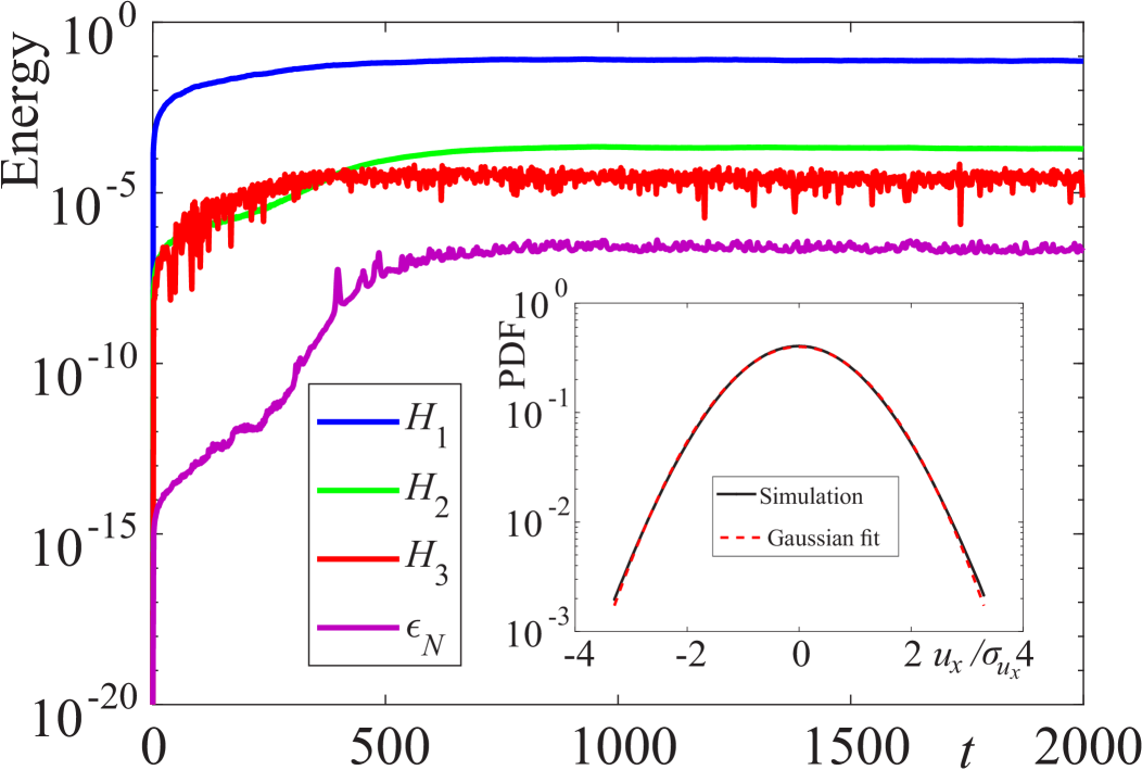
Figure 1: Energy contributions (10) and energy flux (25) are shown as a function of time for $a=2.5\cdot 10^{-3}$. The inset shows the probability density function (PDF) for $u_{x}$ measured relative to the standard deviation $\sigma_{u_{x}}$. The red dashed lines correspond to a Gaussian distribution.

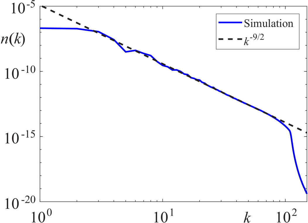
Figure 2: Spatial spectrum of wave action $n(k)$, calculated in the steady state, for the regime of weak dispersion $a=2.5\cdot 10^{-3}$. The black dotted line corresponds to the Zakharov-Sagdeev spectrum (3).

The second numerical experiment was aimed at testing the possible realization of the weak turbulence regime in the complete absence of dispersion, i.e., at $a=0$. Fig. 3 shows that the system of non-dispersive acoustic waves reaches a stationary state at approximately the same time ($t\approx 500$) as in the case of weak dispersion. The intensity of energy pumping $F_{0}$ was the same for both numerical experiments, $F_{0}=1.25\cdot 10^{-3}$. The term responsible for the nonlinear interaction $H_{3}$ turns out to be three orders of magnitude smaller than the linear energy $H_{1}$ in this regime. The corresponding probability density for the quantity $u_{x}$, shown in the inset to Fig. 3, is close to the Gaussian distribution, as in the weakly dispersive case. Fig. 4 shows the turbulence spectrum for the non-dispersive regime $a=0$. The calculated wave action spectrum is in very good agreement with the spectrum of Zakharov-Sagdeev $k^{-9/2}$ (3), written in terms of $n_{k}$. Thus, upon transition to the non-dispersive regime, the system remains in a weakly turbulent state. The question arises: what is the mechanism for the realization of weak acoustic turbulence in the absence of wave dispersion? To answer this question, Fig. 5 shows the Fourier isosurfaces of the spectra for two regimes. It can be seen that in the non-dispersive regime, see Fig. 5 (b), structures with a large number of jets in the form of narrow cones arise in the distribution of turbulent pulsations. The emergence of such structures is the result of resonant wave interactions (1). In the weakly dispersive regime, jets are observed only at very small $k$, close to the pumping region, when dispersion can be neglected. In the region of large wave numbers, jets are smoothed out, and the spectrum distribution correspondingly tends to be isotropic, shown in Fig. 5 (a). In the absence of dispersion, such smoothing does not occur and the spectrum is a discrete set of narrow jets.

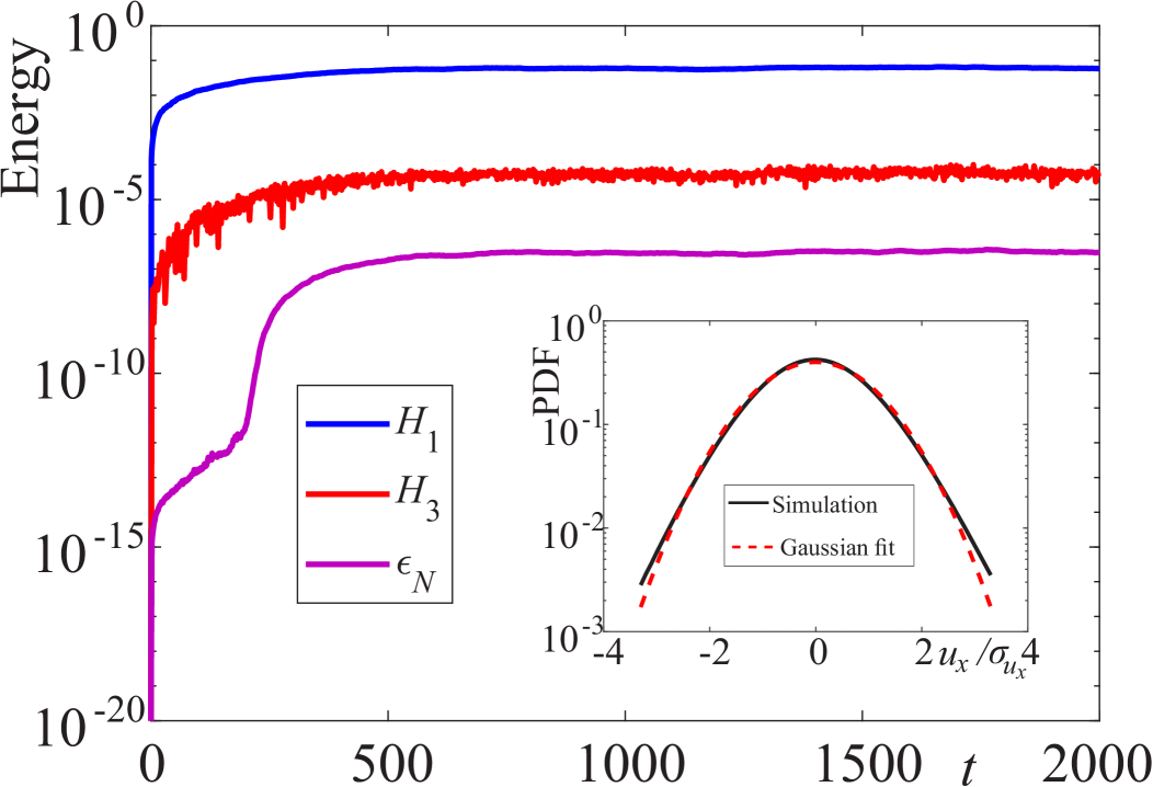
Figure 3: Energy contributions (10) and energy flux (25) are shown as a function of time for $a=0$. The inset shows the probability density function (PDF) for $u_{x}$ measured relative to the standard deviation $\sigma_{u_{x}}$. The red dotted lines correspond to a Gaussian distribution.

Figure 4: Spatial spectrum of wave action $n(k)$, calculated in the steady state, for the dispersionless regime $a=0$. The black dotted line corresponds to the Zakharov-Sagdeev spectrum (3).

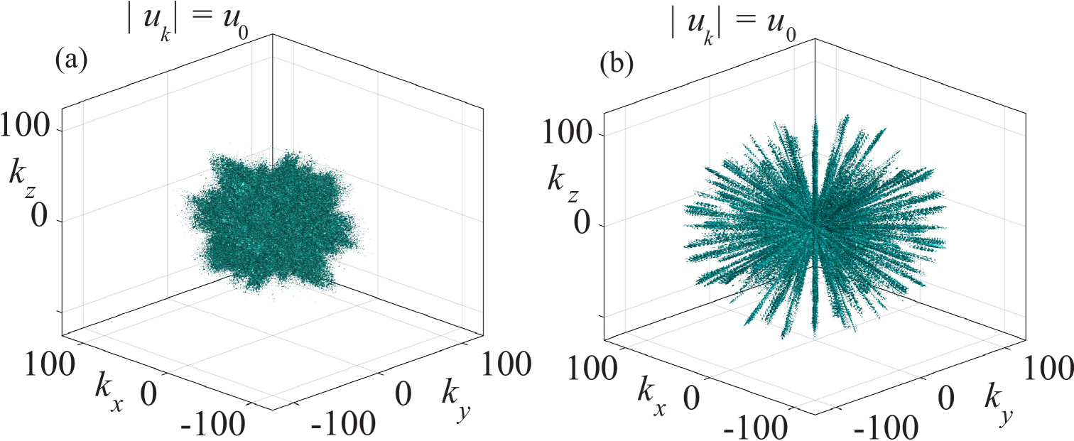
Figure 5: Isosurfaces of the Fourier spectrum $|u_{k}|=5\cdot 10^{-6}$ (a) for $a=2.5\cdot 10^{-3}$ and (b) $a=0$.

To clarify the mechanism of weak turbulence in the non-dispersive regime, a separate jet directed along the $x$ axis was isolated using filtering in the Fourier space. For such a narrow cone (jet), the dispersion relation (2) ($a=0$) can be expanded in a series with respect to the small parameter $\Omega_{0}=k_{\perp}/k_{x}$ (the cone angle):

$$\omega_{k}=|\mathbf{k}|\approx k_{x}\left(1+\Omega_{0}^{2}/2\right),$$

so that $H_{1}$ is the sum of two terms

$$H_{1}=\int\omega_{k}n(k)d\mathbf{k}\approx\int{[k_{x}+\Omega_{0}^{2}k_{x}/2]n(k)d\mathbf{k}}=H_{\parallel}+H_{\perp},$$

where $H_{\parallel}$ is the energy of the acoustic beam propagating along the $x$ direction, and $H_{\perp}$ determines its diffraction energy. To calculate these contributions, we filtered the function $u(\mathbf{k})$ in a narrow cone along $k_{x}$ with an apex angle of $\Omega_{0}=\pi/10$. The result of such filtering is shown in Fig. 6. Thus, the energy contributions have the ratio $H_{\perp}/H_{\parallel}\approx 0.05$. Direct calculation gives $H_{\perp}\approx 4.3\cdot 10^{-5}$, while the energy of nonlinear interaction for the selected cone is estimated as $H_{3}\approx 3.7\cdot 10^{-7}$. Thus, for an individual jet, the diffraction energy turned out to be two orders of magnitude greater than the energy of nonlinear interaction, which explains the occurrence of weak acoustic turbulence.

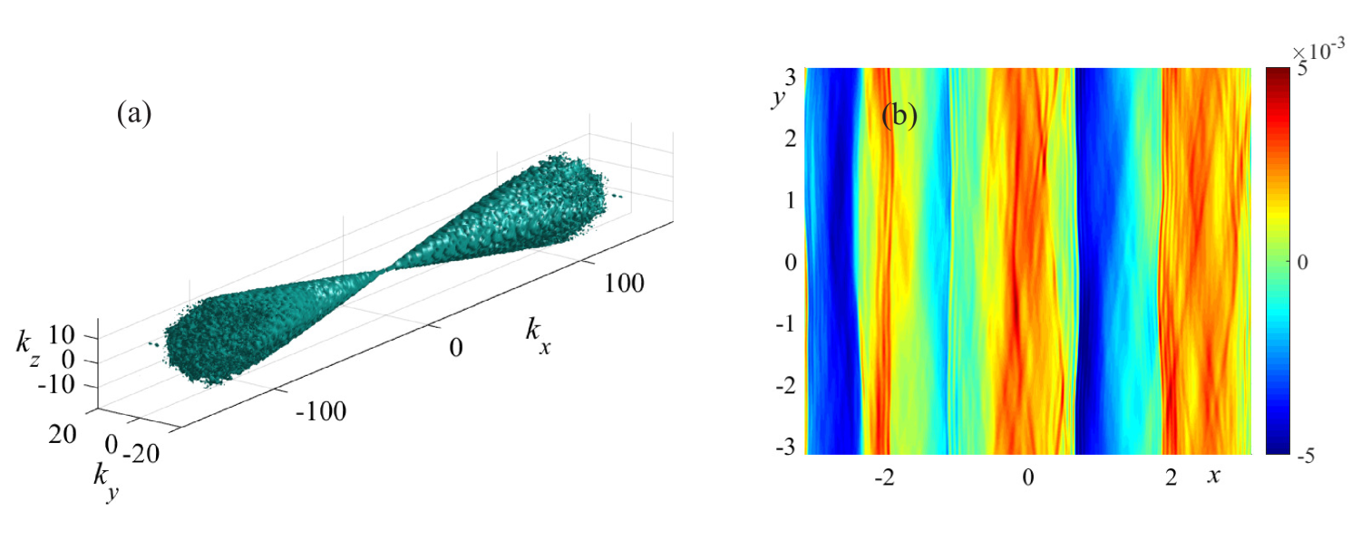
Figure 6: (a) Isosurface of the Fourier spectrum $|u(\mathbf{k})|=10^{-7}$ for a single jet inside the angle $\pi/10$. (b) The inverse Fourier transform of the jet in the $\{x,y\}$ plane at time $t=2000$, corresponding to the quasi-stationary state, is shown.

Thus, weak acoustic turbulence can be realized both in the weak dispersion regime and in the completely non dispersion case. The criterion for the realization of weak turbulence in both regimes is in some sense the same: the effects of dispersion or diffraction (in the case of $a=0$) should prevail over the nonlinearity, which is responsible for the breaking of acoustic waves. An important characteristic of the weakly turbulent regime of acoustic turbulence is the Kolmogorov-Zakharov constant $C_{KZ}$, which is part of the spectrum (3). For its numerical evaluation, we carried out two series of calculations for weakly dispersion and non dispersion regimes of wave turbulence. The numerical experiments simulated decaying turbulence at $F_{0}=0$. The initial conditions were taken at the time $t=2000$, corresponding to the quasi-stationary state. The calculations were performed on the time interval $T=1000$. As can be seen from Fig. 7, during this period of time the total energy decreases by several times, and the dissipation flow almost stops, i.e., the system becomes almost linear. In the mode of decaying turbulence, the evolution of the turbulence spectra is self-similar with the preservation of the exponent $-9/2$, but the coefficient before the power decreases with time as a result of energy dissipation. To estimate the Kolmogorov-Zakharov constant, we present the calculated energy spectra in the form $E(k)=C_{k}k^{-3/2}$, where the value of $C_{k}$ was calculated for two modes depending on the energy flow $\epsilon$. The measured functions agree well with the analytical dependence $C_{k}\propto\epsilon^{1/2}$, both for weakly dispersive and for non-dispersive regimes, see Fig. 8. The insets to Fig. 8 allow us to directly estimate the values of the constants for two regimes: $C_{KZ}\approx 0.24$ (weakly dispersive) and $C_{KZ}\approx 0.1$ (non-dispersive). Thus, the numerical estimate for the Kolmogorov-Zakharov constant in the weakly dispersive regime agrees much better with the exact value $C_{KZ}\approx 0.22$. In the non-dispersive regime, the value of $C_{KZ}$ differs from (22) by approximately a factor of two. Apparently, such a difference arises as a result of the anisotropic distribution of energy in the Fourier space, observed in Fig. 5 (b). In the presence of dispersion, the turbulence spectrum tends to an isotropic distribution, providing a value of the Kolmogorov-Zakharov constant closer to the theoretical value (22).

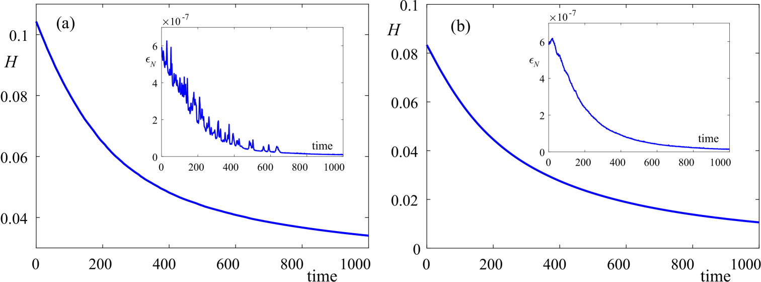
Figure 7: Evolution of the total energy for (a) $a=2.5\cdot 10^{-3}$ and (b) $a=0$. The insets show the time dependence of the energy dissipation flux.

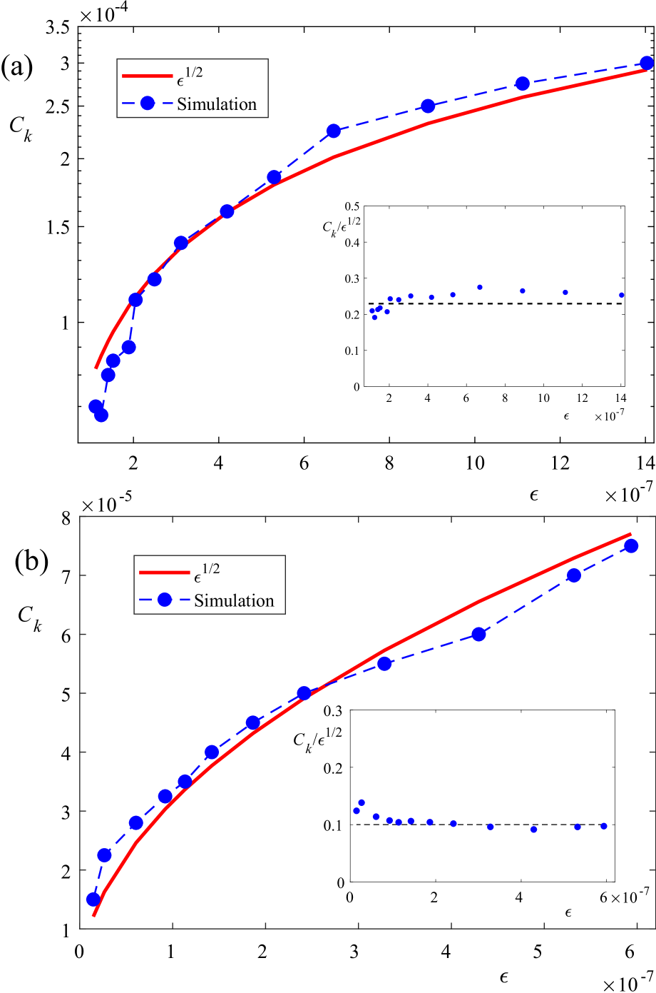
Figure 8: The $C_{k}$ coefficients are shown as functions of the measured energy flux for (a) $a=2.5\cdot 10^{-3}$ and (b) $a=0$. The red solid lines show the square root $\epsilon^{1/2}$ dependence. The insets show the compensated $C_{k}/\epsilon^{1/2}$ (Kolmogorov-Zakharov’s constant) values.

Let us now consider the last third series of calculations. The goal of this part of the work was to simulate the non-dispersive regime of wave turbulence, but with an increase in the level of nonlinearity of the system. For this purpose, the pumping amplitude $F_{0}$ was significantly increased to $40\cdot 10^{-3}$, i.e., more than an order of magnitude greater compared to the two previous numerical experiments. For such conditions we observed a very fast transition to the steady state, in times $t\approx 50$, see Fig. 9. In the inset to Fig. 9 one can see that the probability density function is very different from the Gaussian distribution with strongly elongated non-Gaussian tails, indicating the presence of extreme events (shock waves). Note that for the one-dimensional Burgers equation with weak viscosity and random pumping, the tails of the probability density function for the velocity gradient decay according to a power law with exponent $-7/2$, see details [34, 35, 36, 37, 38, 39]. In the inset in Fig. 9, it can be seen that the calculated probability density for $u_{x}$ is described with high accuracy by the same power-law dependence: $|u_{x}|^{-7/2}$. Thus, Fig. 9 indicates a high level of intermittency in the system. The turbulence spectrum for a strongly nonlinear regime is shown in Fig. 10: the exponent for $n(k)$ is close to $-5$, which in terms of wave action corresponds to the Kadomtsev-Petviashvili (4) spectrum. Fig. 11 shows the spatial distribution of $u(\mathbf{r})$ in the $z=0$ plane. It can be clearly seen that a large number of discontinuities have formed in the distribution of $u(\mathbf{r})$. In fact, such discontinuities are a set of shock waves, propagating at different angles to each other. Thus, at a large pumping amplitude, a transition to a state of strong acoustic turbulence is indeed observed, described by the Kadomtsev-Petviashvili spectrum (4) and representing an ensemble of shock waves chaotically propagating in space due to the random nature of the system pumping.

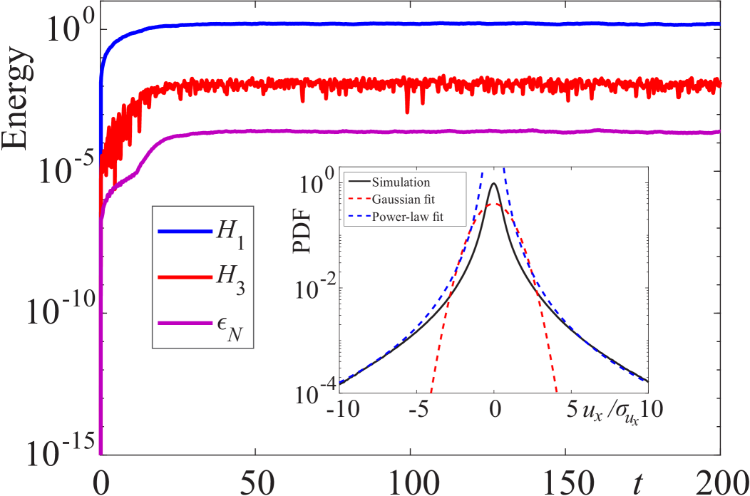
Figure 9: Energy contributions (10) and energy flux (25) are shown as a function of time for $a=2.5\cdot 10^{-3}$. The inset shows the probability density function (PDF) for $u_{x}$ measured relative to the standard deviation $\sigma_{u_{x}}$. The red dotted lines correspond to a Gaussian distribution, the blue dotted lines to a power law: $|u_{x}/\sigma_{u_{x}}|^{-7/2}$.

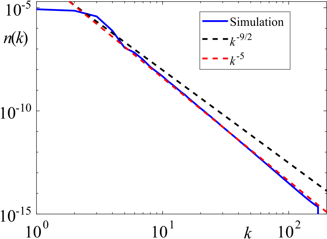
Figure 10: Spatial spectrum of wave action $n(k)$, calculated in the steady state, for the non-dispersive regime $a=0$. The black dotted line corresponds to the Zakharov-Sagdeev spectrum (3), the red dotted line is the Kadomtsev-Petviashvili spectrum (4).

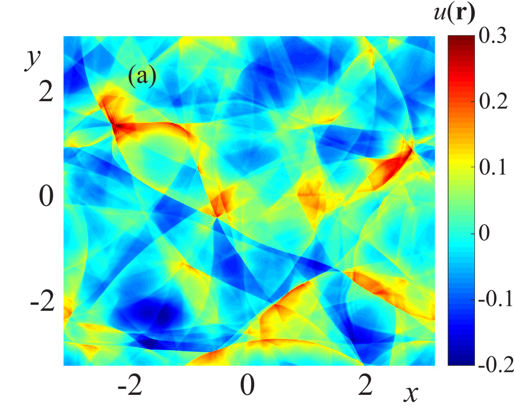
Figure 11: Distribution of the quantity $u(\mathbf{r})$ in the plane $z=0$ in the regime of strong acoustic turbulence.

V Conclusion

In this, review we have presented the research results on three-dimensional sound turbulence. This study includes both analytical investigations going back to the works of Zakharov and Sagdeev on weak wave turbulence [12, 13] and to the work of Kadomtsev and Petviashvili [14] on strong sound turbulence. The main results of this review were recently published by the authors in [15, 16] Based on the direct numerical simulation technique, it was found that the transition from a weakly turbulent regime to strong turbulence is determined by the ratio of linear (dispersion or diffraction) effects to nonlinearity. A numerical experiment confirmed the existence of weak sound turbulence with the Zakharov-Sagdeev spectrum ($~k^{-3/2}$) for both weak positive dispersion waves and non-dispersive sound waves. The calculations revealed that the spectrum of weak sound turbulence is strongly anisotropic, especially in the region of small $k$, where the distribution in $k$-space consists of a set of jets. In the weak positive dispersion regime, the jets broaden with increasing $k$ and the spectrum becomes almost isotropic. For non-dispersive sound waves, the distribution in Fourier space is a finite number of cone-shaped jets, for each of which diffraction across the jets prevents the breaking of sound waves, realizing the weak sound turbulence regime. In other words, diffraction plays the same role in this case as dispersion. It should be noted that for weak nonlinearity each jet in the non-dispersive limit $a=0$ can be described by the Khokhlov-Zabolotskaya equation [40], which describes the competition between the nonlinear interaction and beam diffraction. In our numerical experiments, when the weakly turbulent Zakharov-Sagdeev spectrum is realized, diffraction effects dominate. In the strongly nonlinear turbulent regime, the jet structure disappears and the spectrum turns out to be close to isotropic due to shock waves propagating at different angles (see Fig. 11). The formation of shock waves in sound beams described by the Khokhlov-Zabolotskaya equation was also observed in numerical simulations (see the review [41] and references therein). However, the distribution remained quasi-one-dimensional.

In weak turbulence, the probability density distribution of wave field gradients turns out to be close to Gaussian. In the regime of strong nonlinearity for sound waves without dispersion, the main effects are the breaking and formation of shock waves. This is the reason for the formation of Kadomtsev-Petviashvili spectrum. In this case, power-law tails for large deviations of the gradient appear in the probability density distribution (PDF), similar to those predicted by the Burgers turbulence theory with an index close to $-7/2$. Such tails indicate the intermittency of Kadomtsev-Petviashvili turbulence. Thus, the sound turbulence is transformed into an ensemble of random shock waves, and is described with high accuracy by the Kadomtsev-Petviashvili spectrum (4). The calculations are based on pseudo-spectral methods of direct numerical modeling of acoustic turbulence. Simulations were carried out in a wide range of control parameters and allowed to establish criteria for the formation of a weak or strong turbulent regime. Thus, the Zakharov-Sagdeev (3) and Kadomtsev-Petviashvili (4) spectra correspond to different limiting cases of weakly and strongly nonlinear regimes of three-dimensional acoustic turbulence with respect to linear wave effects.

In conclusion, we would like to discuss when power-law ($~k^{-3/2}$) turbulent spectra of sound-type waves arise. As noted above, the numerical experiment [7] for turbulence of fast magnetosonic waves in plasma with small $\beta$ demonstrates the Zakharov-Sagdeev spectrum, since waves of this type have the sound dispersion law $\omega=kV_{A}$ (here $V_{A}$ is the Alfvén velocity) in the frequency range below the ion cyclotron $\omega_{ci}$. The spectrum of slow magnetosonic waves (in plasma with small $\beta$ they can be considered as magnetized ion sound) demonstrates the same dependence on $k$ as the Zakharov-Sagdeev spectrum, corresponding to a constant energy flow into the region of short waves, despite strong anisotropy. For small $\beta$, the same dependence on the modulus $k$ is shown by the spectra of weak turbulence of fast magnetosonic and Alfvén waves interacting with slow magnetosonic waves [43]. Recent experiments (see the papers [44, 45] and references therein) on observing the spectra of magnetic field fluctuations in the solar wind near the Sun have shown dependencies close to the spectrum $~\omega^{-3/2}$, where the parameter $\beta$ is small, of the order of $0.1$. The Kadomtsev-Petviashvili spectrum, as shown by numerical experiments [46] with applications to astrophysics, is often encountered in MHD turbulence, as is the spectrum $~k^{-3/2}$. It is important that the anisotropy of the spectra due to the magnetic field does not affect the dependence of the spectra on the absolute value of $k$. For weak MHD turbulence, this behavior follows from simple dimensional estimates.

VI Acknowledgements

The authors express their sincere gratitude to V.E. Zakharov for fruitful discussions at the early stage of this work. We are grateful to S.N. Gurbatov, who drew our attention to the articles on Burgers turbulence [34]-[39], and to R.Z. Sagdeev, who pointed out the numerical modeling of MHD wave turbulence in astrophysics. The work was supported by the Russian Science Foundation (grant: 19-72-30028)

References

- [1] Zakharov V.E., L’vov V.S., Falkovich G. Kolmogorov Spectra of Turbulence I: Wave Turbulence: Berlin Springer-Verlag, 1992. 264 p.
- [2] Nazarenko S. Wave Turbulence: Springer Berlin Heidelberg, series: Lecture Notes in Physics, 2011. 279 p.
- [3] Griffin A., Krstulovic G., L’vov V.S., Nazarenko S. Energy spectrum of two-dimensional acoustic turbulence //Physical Review Letters. 2022. V 128. No. 22. Art. no. 224501. doi: 10.1103/PhysRevLett.128.224501
- [4] Shavit M., Falkovich G. Singular measures and information capacity of turbulent cascades //Physical Review Letters. 2020. V. 125. No. 10. Art. no. 104501. doi: 10.1103/PhysRevLett.125.104501
- [5] Frahm K. M., Shepelyansky D. L. Random matrix model of Kolmogorov-Zakharov turbulence //Physical Review E. 2024. V. 109. No. 4. Art. no. 044201. doi: 10.1103/PhysRevE.109.044201
- [6] Semisalov B. V. et al. Numerical analysis of the kinetic equation describing isotropic 4-wave interactions in non-linear physical systems //Communications in Nonlinear Science and Numerical Simulation. 2024. V. 133. Art. no. 107957. doi: 10.1016/j.cnsns.2024.107957
- [7] Galtier S. Fast magneto-acoustic wave turbulence and the Iroshnikov–Kraichnan spectrum //Journal of Plasma Physics. 2023. V. 89. No. 2. Art. no. 905890205. doi: 10.1017/S0022377823000259
- [8] Hindmarsh M. et al. Gravitational waves from the sound of a first order phase transition //Physical Review Letters. 2014. V. 112. No. 4. Art. no. 041301. doi: 10.1103/PhysRevLett.112.041301
- [9] Galtier S. A multiple time scale approach for anisotropic inertial wave turbulence //Journal of Fluid Mechanics. 2023. V. 974. P. A24. doi: 10.1017/jfm.2023.825
- [10] Kalaydzhyan T., Shuryak E. Gravity waves generated by sounds from big bang phase transitions //Physical Review D. 2015. V. 91. No. 8. Art. no. 083502. doi: 10.1103/PhysRevD.91.083502
- [11] Falcon E., Mordant N. Experiments in surface gravity–capillary wave turbulence //Annual Review of Fluid Mechanics. 2022. V. 54. No. 1. P. 1-25. doi: 10.1146/annurev-fluid-021021-102043
- [12] Zakharov V. E. Weak turbulence in media with a decay spectrum //Journal of Applied Mechanics and Technical Physics. 1965. V. 6. No. 4. P. 22-24. doi: 10.1007/BF01565814
- [13] Zakharov V. E., Sagdeev R. Z. Spectrum of acoustic turbulence // Soviet Physics Doklady. 1970. V. 15. P. 439.
- [14] Kadomtsev B. B., Petviashvili V. I. On acoustic turbulence // Soviet Physics Doklady. 1973. V. 208. No. 4. P. 794-796.
- [15] Kochurin E. A., Kuznetsov E. A. Direct numerical simulation of acoustic turbulence: Zakharov–Sagdeev spectrum //JETP Letters. 2022. V. 116. No. 12. P. 863-868. doi: 10.1134/S0021364022602494
- [16] Kochurin E. A., Kuznetsov E. A. Three-Dimensional Acoustic Turbulence: Weak Versus Strong //Physical Review Letters. 2024. V. 133. No. 20. Art. no. 207201. doi: 10.1103/PhysRevLett.133.207201
- [17] Newell A. C., Aucoin P. J. Semidispersive wave systems //Journal of Fluid Mechanics. 1971. V. 49. No. 3. P. 593-609. doi: 10.1017/S0022112071002271
- [18] L’vov V. S. et al. Statistical description of acoustic turbulence //Physical Review E. 1997. V. 56. No. 1. P. 390. doi: 10.1103/PhysRevE.56.390
- [19] Dyachenko S., Newell A. C., Pushkarev A., Zakharov V. E. Optical turbulence: weak turbulence, condensates and collapsing fragments in the nonlinear Schrodinger equation // Physica D. 1992. V. 57. P. 96-160. doi: 10.1016/0167-2789(92)90090-A
- [20] Benney D. J., Saffman P. G. Nonlinear interactions of random waves in a dispersive medium //Proceedings of the Royal Society of London. Series A. Mathematical and Physical Sciences. 1966. V. 289. No. 1418. P. 301-320. doi: 10.1098/rspa.1966.0013
- [21] Zakharov V. E., Musher S.L. Kolmogorov spectrum in a system of nonlinear oscillators// Soviet Physics Doklady. 1973. V. 209. P. 1063-1065.
- [22] Connaughton C. Numerical Solutions of the Isotropic 3-Wave Kinetic Equation. // Physica D. V. 238. P. 2282-2297. doi.org/10.1016/j.physd.2009.09.012
- [23] Connaughton C., Krapivsky P.L. Aggregation?fragmentation processes and decaying three-wave turbulence // Phys. Rev. E. 2010. V. 81, 035303(R). doi.org/10.1103/PhysRevE.81.035303
- [24] Zakharov V. E., Kuznetsov E. A. Solitons and collapses: two evolution scenarios of nonlinear wave systems //Physics-Uspekhi. 2012. V. 55. No. 6. P. 535. doi: 10.3367/UFNe.0182.201206a.0569
- [25] Kuznetsov E. A. Instability of solitons and collapse of acoustic waves in media with positive dispersion // JETP. 2022. V.13. P. 121–135] doi: 10.1134/S1063776122060103
- [26] Kuznetsov E. A. Turbulence spectra generated by singularities //Journal of Experimental and Theoretical Physics Letters. 2004. V. 80. P. 83-89. doi: 10.1134/1.1804214
- [27] Burgers J. M. A mathematical model illustrating the theory of turbulence //Advances in applied mechanics. 1948. V. 1. P. 171-199. doi: 10.1016/S0065-2156(08)70100-5
- [28] Kuznetsov E.A., Kochurin E.A. Sound turbulence: from the Zakharov–Sagdeev spectra to the Kadomtsev–Petviashvili spectrum, XXI Scientific School ”Nonlinear Waves - 2024”, Nizhny Novgorod, November 5-11, 2024.
- [29] Zakharov V. E., Kuznetsov E. A. Hamilton formalism for nonlinear waves //Physics-Uspekhi. 1997. V. 40. No.11. P. 1087-1116. doi: 10.1070/PU1997v040n11ABEH000304
- [30] Zakharov V. E. On stochastization of one-dimensional chains of nonlinear oscillators// Sov. Phys.-JETP. 1974. V. 38. No.1, P. 108-110.
- [31] Peierls, R. Zur kinetischen theorie der wärmeleitung in kristallen. Annalen der Physik, 1929. V. 395. No 8. P. 1055-1101.
-
[32]
Landau, L., Rumer, G. Uber schall absorption in festen Korpen.
Phys. Z. Sowjetunion, 1937. V. 11. P. 18-25. - [33] Landau L.D., Lifshitz E.M. Fluid Mechanics: Oxford: Pergamon Press, 1987. 135 p.
- [34] Gurbatov S.N., Malakhov A.N., Saichev A.I. Nonlinear random waves and turbulence in nondispersive media: waves, rays, particles. Manchester University Press. 1991. P. 308
- [35] Yakhot V., Chekhlov A. Algebraic tails of probability density functions in the random-force-driven Burgers turbulence // Physical Review Letters. 1996. V. 77. N. 15. P. 3118. doi: 10.1103/PhysRevLett.77.3118
- [36] Weinan E., Eijnden E. V. Asymptotic theory for the probability density functions in Burgers turbulence // Physical Review Letters. 1999. V. 83. N. 13. P. 2572. doi: 10.1103/PhysRevLett.83.2572
- [37] Frisch, U., Bec J. Burgulence. In New trends in turbulence Turbulence: nouveaux aspects. Berlin, Heidelberg: Springer Berlin Heidelberg. 2002. P. 341.
- [38] Bec J., Khanin K. Burgers turbulence // Physics Reports. 2007. V. 447. N. 1-2. P. 1-66. doi: 10.1016/j.physrep.2007.04.002
- [39] Frisch U., Bec J., Villone B. Singularities and the distribution of density in the Burgers/adhesion model //Physica D: Nonlinear Phenomena. 2001. V. 152. P. 620-635. doi: 10.1016/S0167-2789(01)00195-6
- [40] Zabolotskaya, E. A., Khokhlov R.V. Quasi-plane waves in the nonlinear acoustics of confined beams // Sov. Phys. Acoust. 1969. V. 15(1). P. 35-40.
- [41] Rudenko, O. V. The 40th anniversary of the Khokhlov-Zabolotskaya equation // Acoustical Physics, 2010 V. 56. P. 457-466.
- [42] Kuznetsov E.A. Turbulence of Ion Sound in a Plasma Located in a Magnetic Field// Soviet Physics JETP. 1972. V. 35. No. 2. P. 310-314.
- [43] Kuznetsov E.A. Weak Magnetohydrodynamic Turbulence of a Magnetized Plasma// JETP. 2001. V. 93, No. 5. P. 1052.
- [44] Chen, C. H. K. et al. The evolution and role of solar wind turbulence in the inner heliosphere // The Astrophysical Journal Supplement Series. 2020. V. 246. No. 2. P. 53. doi: 10.3847/1538-4365/ab60a3
- [45] Šafránková J. et al. Evolution of Magnetic Field Fluctuations and Their Spectral Properties within the Heliosphere: Statistical Approach // Astrophysical Journal Letters. 2023. V. 946. No. L44. https://doi.org/10.3847/2041-8213/acc531
- [46] Popova E., Lazarian A. Outlook on Magnetohydrodynamical Turbulence and Its Astrophysical Implications// Fluids. 2023. V. 8. No. 5. P. 142. https://doi.org/10.3390/fluids8050142