Fast approximative estimation of conditional Shapley values when using a linear regression model or a polynomial regression model

Abstract

We develop a new approximative estimation method for conditional Shapley values obtained using a linear regression model. We develop a new estimation method and outperform existing methodology and implementations. Compared to the sequential method in the shapr-package (i.e fit one and one model), our method runs in minutes and not in hours. Compared to the iterative method in the shapr-package, we obtain better estimates in less than or almost the same amount of time. When the number of covariates becomes too large, one can still fit thousands of regression models at once using our method. We focus on a linear regression model, but one can easily extend the method to accommodate several types of splines that can be estimated using multivariate linear regression due to linearity in the parameters.

1 Introduction

We introduce an efficient procedure for the estimation of conditional Shapley values when we have mixed type of covariates and we want to use a linear explainer to obtain the Shapley values. The linear explainer fits multiple linear regression models with different subsets of covariates to the predictions of the model. This technique accounts for covariate dependence when estimating the Shapley values. However, when using exact calculations, the number of models that needs to be estimated is $2^{p}$ models, which becomes more and more computationally demanding to estimate when the number of covariates, $p$, becomes large. In this paper we show that we can fit thousands of different linear regression models approximately at the same time and do this relatively fast. We need to exploit the sparseness of the joint precision matrix. Sparse matrix algebra exploits that the matrix involved has many 0s.

We derive a result that has an approximative expression as solution and use this result to derive a fast estimation procedure. The result states that one can fit submodels of a linear regression model approximately by adding large numbers to the diagonal of the precision (i.e. inverse covariance) matrix of the original model with all covariates.

The paper is structured as follows. In Section 2 we give an introduction to Shapley values, in Section 3 we introduce constrained Gaussian Markov Random Fields, which is the backbone of our methodology. In Section 4 we derive the result and derive an efficient estimation procedure. In Section 5 we provide a numerical example, where we consider a subset of the covariates in the WHO Life Expectancy dataset. In Section 6 we provide a discussion and also a conclusion.

2 Brief overview of Shapley values used to explain individual model predictions

The Shapley value (Shapley, 1953) originates from game theory and is used to distribute payoff to the players of a game based on their contributions. In machine learning it is used to tell how much the different features contributed to a specific prediction of a model. We now formalize this.

Assume we want to explain a prediction of a model $f(\bm{x})$ trained on $\mathcal{X}=\{\bm{x}^{[i]},y^{[i]}\}_{i=1}^{N_{train}}$, where $\bm{x}_{i}$ is an $p$-dimensional feature vector, $y^{[i]}$ is a univariate response and the number of training observations is $N_{train}$. The prediction $\hat{y}=f(x)$ for a feature vector $\bm{x}=\bm{x}^{*}$ is to be explained by using Shapley values. Denote the Shapley value corresponding to feature $i$ for $\phi_{i}$. The Shapley value vector $\bm{\phi}$ is a break-down of the prediction into the contribution of each of the predictors. This means $\phi_{i}$ tells us how much the $i$-th feature contributed to the specific prediction of a model in a positive (positive value) or negative way (negative value).

To calculate $\bm{\phi}$ we need to define what is called the contribution function, which should resemble the value of $f(\bm{x}^{*})$ when only the features in coalition $S$ are known. We use the contribution function (Lundberg and Lee, 2017)

$$v(S)=E(f(\bm{x})|\bm{x}_{s}=\bm{x}_{s}^{*}),$$ (1)

which means we consider the expected value of $f(x)$ conditioned on the features in $S$ taking on the values $\bm{x}^{*}$. For instance when $S$ consists of the first two features, then the conditional expectation is conditional on these two features only and at the specified values. We must calculate the contributions for each possible configuration of covariates to be able to find the Shapley values. For $p$ features, there are $2^{p}$ possible subsets, which means the procedure becomes non-doable when then there are many features. The conditional expectation function provides a summary of the whole distribution and is the most commonly used estimation of $f$ in prediction analysis.

We use the so called Kernel SHAP procedure so that we estimate $\bm{\phi}$ by solving a linear weighted least squares problem. The shapley values $\bm{\phi}$ is obtained by solving the system of equations

$$\bm{Z}^{T}\bm{W}\bm{Z}\bm{\phi}=\bm{Z}^{T}\bm{W}\bm{v},$$ (2)

here $\bm{v}$ is the vector of expected contribution function of length $2^{p}$, $\bm{Z}$ is a $2^{p}\times(p+1)$ binary matrix (0 and 1), where the first coloumn is a coloumn vector of 1s and the $i$ element in the j-th row is 1 if covariate $i$ is in the set $S$ corresponding to the $j$-th value of contribution function and otherwise 0, and the weight matrix $\bm{W}$ is a diagonal matrix $2^{p}\times 2^{p}$ with elements $k(p,|S|)=(p-1)/\binom{N}{k}|S|(p-|S|)$. Here $|S|$ is the number of covariates in the set $S$. We set $k(p,0)$ and $k(p,p)$ to $10^{6}$, which is also done in the shapr-package (Jullum et al., 2025).

There are mainly two ways to estimate $v(S)$, Monte Carlo methods and regression methods. The Monte Carlo methods use sampling to estimate the conditional expectation. The regression paradigm directly fits a regression model that predicts $v(S)$. We focus only on the regression paradigm in our work.

When the number of covariates becomes large, one can also sample the subsets (with replacement), which are also called coalitions, used to estimate $\bm{\phi}$. One uses the Shapley weights $k(p,S)$ as sampling weights and always include the empty and full coalitions in the estimation.

There is also a popular Shapley value called the marginal Shapley value. The term marginal stems from the fact that it does not take into account feature dependence in the estimation phase. The first paper to take into account feature dependence is Aas et al. (2021), and the corresponding Shapley value is the conditional one. The shap package (Lundberg and Lee, 2017) is a highly popular package used to estimate (mainly) marginal Shapley values, while shapr (Jullum et al., 2025) estimates conditional Shapley values. In general the shapr-package is to some extent slower since it takes into account feature dependence.

More details on Shapley value estimation and background theory for prediction models is given in e.g Lundberg and Lee (2017), Aas et al. (2021) or Olsen et al. (2024).

3 Constrained Gaussian Markov Random Fields

In this section we provide a short summary of constrained Gaussian Markov Random Fields. The theory is needed in the development of the new theory.

A multivariate random variable $\bm{x}$ is said to be a Gaussian Markov Random Field if the density is given by (Rue and Held, 2005, p. 22)

$$f(x)=(2\pi)^{-n/2}|\bm{Q}|^{1/2}\exp\big{(}-\frac{1}{2}(\bm{x}-\bm{\mu})^{T}(\bm{x}-\bm{\mu})\big{)},$$ (3)

where $\bm{\mu}$ is the mean vector and $\bm{Q}$ is the precision matrix. The parameter $\tau$ is a hyper-parameter called the precision parameter, and is connected to the variance parameter by $\tau=1/\sigma^{2}$. It is a well-known fact that the parameter estimates in the multivariate linear regression is gaussian conditional on the hyperparameter $\tau$ of the observations. The estimated mean is given by

$$\bm{\mu}=(\bm{X}^{T}\bm{X})^{-1}\bm{X}^{T}\bm{Y},$$ (4)

and the precision matrix is given by $\bm{Q}=\bm{X}^{T}\bm{X}\tau$,

The distribution of $\bm{x}$ under linear constraints $\bm{A}\bm{x}=\bm{0}$ can be obtained by considering the distribution of $(\bm{x},\bm{A}\bm{x})$ and then conditioning on $\bm{A}\bm{x}$ using standard multivariate normal distribution theory. One obtains that

$$\bm{\Sigma}^{*}=\bm{Q}^{-1}-\bm{Q}^{-1}\bm{A}^{T}(\bm{A}\bm{Q}^{-1}\bm{A}^{T})^{-1}\bm{A}\bm{Q}^{-1},$$ (5)

and

$$\bm{\mu}^{*}=\bm{\mu}-\bm{Q}^{-1}\bm{A}^{T}(\bm{A}\bm{Q}^{-1}\bm{A}^{T})^{-1}\bm{A}\bm{\mu}.$$ (6)

By comparing the two above equations, we have that

$$\bm{\mu}^{*}=\bm{\Sigma}^{*}\bm{Q}\bm{\mu}.$$ (7)

We call the above equations for the correction equations, as we correct the original parameters (mean vector and covariance matrix) for the constraints.

In the regression setting, we impose several constraints. Call the i-th constraint for $\bm{A}_{i}$ and where the i-th element is 1 if we set the regression coefficient to 0. This is equivalent to imposing the so-called corner constraint. Here we split the $\bm{x}$ vector in two, $\bm{x}_{A}$ and $\bm{x}_{B}$ and condition the vector $\bm{x}_{A}$ on $\bm{x}_{B}=0$. Partition the precision matrix as follows

$$\begin{bmatrix}\bm{Q}_{A}&\bm{Q}_{AB}\\ \bm{Q}_{BA}&\bm{Q}_{B}\end{bmatrix}.$$ (8)

From Theorem 2.5 in Rue and Held (2005), the precision matrix under the corner constraint is $\bm{Q}_{A}$. This means we can obtain the precision matrix of a smaller model by removing coloumns from the original model matrix $\bm{X}$. An alternative derivation can be made by using that the corner parametrization is equivalent to introducing a projection matrix $\bm{P}=\bm{I}-\sum\bm{A}_{i}\bm{A}_{i}^{T}=\bm{I}-\bm{D}$, where $\bm{D}$ is a diagonal matrix where element $(j,j)$ is 1 if the $j$-th regression coefficient is set to be zero. The precision matrix is given by $\bm{P}\bm{Q}\bm{P}$, and we can safely remove the coloumns of $\bm{X}$ that are set to zero. In the next section we will see that adding large numbers to the diagonal of the original precision matrix approximately gives corner point estimates.

4 Theoretical result and computational algorithm

We now derive the main result of this paper, compare it to another result and state the main problem to be solved by the theorem. In the last subsection we derive the algorithm that is used in the numerical section.

4.1 Main result

The result is a direct consequence of Equation (1) in Henderson and Searle (1981), which states that

$$(\bm{A}+\bm{U}\bm{B}\bm{V})^{-1}=\bm{A}^{-1}-\bm{A}^{-1}\bm{U}(\bm{I}+\bm{B}\bm{V}\bm{A}^{-1}\bm{U})^{-1}\bm{B}\bm{V}\bm{A}^{-1},$$ (9)

By setting $\bm{A}$ in the above equation to $\bm{Q}$ and $\bm{U}$ to $\bm{A}$, $\bm{V}$ to $\bm{A}^{T}$ and $\bm{B}=\bm{I}/\varepsilon$ we obtain

$$\tilde{\bm{\Sigma}}=\bm{\Sigma}-\bm{\Sigma}\bm{A}^{T}(\bm{A}\bm{\Sigma}\bm{A}^{T}+\bm{I}\varepsilon)^{-1}\bm{A}\bm{\Sigma}=(\bm{Q}+\bm{A}\bm{A}^{T}/\varepsilon)^{-1}.$$ (10)

We note that $\bm{A}\bm{\Sigma}\bm{A}^{T}$ has been replaced by $\bm{A}\bm{\Sigma}\bm{A}^{T}+\bm{I}\varepsilon$ in the correction equation for $\bm{\Sigma}^{*}$, which means $\tilde{\bm{\Sigma}}$ is an approximation of $\bm{\Sigma}^{*}$ and which improves, in theory, when $\varepsilon$ becomes smaller and smaller. If $\varepsilon$ is chosen too small, however, it will become numerically 0 due to the finite machine-precision. This means we can approximate the corrected covariance matrix by using $\bm{Q}+\bm{A}\bm{A}^{T}/\varepsilon$ as precision matrix, where $\bm{A}$ is the joint constraint matrix.

4.2 Comparison with other results

In Rue and Held (2005)[p. 39] they derive a result under the assumption of so-called soft constraints, meaning the constraints are observed with noise. If we assume the constraints are observed with gaussian white noise, the precision matrix of the field is $\bm{Q}+\bm{A}\bm{A}\kappa$, but we need to assume that the observed error is $\bm{0}$ to get the correct mean in our result. The soft constraint approximates the hard constraint under these assumptions, and the approximation becomes better and better the smaller the variance of the error term is. By using this result, we are assuming a slightly misspecified model, as the constraints are assumed to be observed with noise. In our result, we make no such assumptions.

In comparison, our result tells us that by directly altering the precision matrix, we approximately perform kriging with hard constraints. By adding $\bm{A}\bm{A}\kappa$ to the precision matrix, we are forcing the precision matrix to have the directions in $A$ as eigenvectors. The variance in these directions becomes small. In general the directions in $\bm{A}$ do not need to be eigenvectors of $\bm{A}$. However, the result justifies adding this correction term to the precision matrix.

4.3 Main problem

Our approximative result can be used to obtain the parameter estimates of the regression parameters in a smaller model by constraining the mean effects in the larger model to be $\bm{0}$.

By replacing $\bm{\Sigma}^{*}$ with $\tilde{\bm{\Sigma}}$ in Equation (7) and canceling out $\tau$, we obtain

$$\bm{\mu}^{*}=(\bm{X}^{T}\bm{X}+\bm{D}/\varepsilon)^{-1}\bm{X}^{T}\bm{y}=\bm{Q}_{S}^{-1}\bm{m},$$ (11)

where $\bm{m}=\bm{X}^{T}\bm{y}$ and $\bm{Q}_{s}=\bm{X}^{t}\bm{X}+\bm{D}/\varepsilon$ This becomes the correcting equations in our setting with a multivariate linear regression model. It should be clear to the reader that we do not calculate the inverse of $\bm{X}^{T}\bm{X}+\bm{D}/\varepsilon$, but instead calculate the Cholesky decomposition of this matrix and solve the corresponding linear system of equations. However, instead of solving each such system iteratively, we estimate all/several of the system of equations jointly, as outlined in Algorithm 1.

If our goal was to estimate a regression model with only one feature, we would be better off by estimating that model and not by correcting the larger model. However, if we want to fit many models, the bookkeeping of coefficients becomes more tedious and time consuming. Also, normally, the precision matrix $\bm{Q}$ is not too big. In space-time models the joint precision matrix with main and interaction effects $\bm{Q}$ can have dimensions 10 000 by 10 000. In our setting, typically $p$ is in the range between 10 and 20, so that $\bm{Q}$ is small, even if some of the covariates are categorical with several categories. This means a joint precision matrix, where several independent models are considered jointly, is very sparse.

Input: Design matrix $\bm{X}$, which means $\bm{Q}=\bm{X}^{T}\bm{X}$, model predictions $\bm{f}$ using the training data, feature vector $\bm{x}^{*}$ to be explained.

Output: Estimated shapley values $\bm{\phi}$ for one or several observations.

Procedure processing: Calculate $\bm{Q}_{r}=\bm{I}_{p}\otimes\bm{Q}$, where $\bm{I}_{p}$ is a $2^{p}\times 2^{p}$ identity matrix and $\bm{Q}=\bm{X}^{T}\bm{X}$. Calculate $\bm{m}$ as $\bm{X}^{T}\bm{f}$ repeated $2^{p}$ times. We now have $\bm{m}$ in Equation (11) but need to find $\bm{Q}_{S}$.

Procedure calculations:

Compute the Cholesky decomposition (or a generalization of it), $\bm{L}$, of $\bm{Q}_{s}=(\bm{Q}_{r}+\bm{D}\kappa)$. Here $\bm{D}$ is a diagonal matrix where element $(i,i)$ is 1 if the coefficient in a model is set to 0. The scalar value $\kappa$ is set to be e.g $\kappa=10^{3}\max_{i}(\bm{Q}_{ii})$, i.e the maximum value of $\bm{Q}$ times $10^{3}$.

 Solve: Equation (11) where $\bm{Q}_{S}$ is used instead of $\bm{Q}_{S}$ as precision matrix. (Note that $\tau$ cancel out when performing the calculations, so it is left out from the calculations).

Obtain $\bm{\phi}$ by solving (2) using the estimated $v$s where we have used $\bm{x}^{*}$ (the observation to be explained) as feature vector.

Algorithm 1 Pseudo-code for fast, approximate Shapley value estimation of linear models.

We implement the code in an R-script (R Core Team, 2025) using native R functions and functions mainly from the Matrix (Bates et al., 2025) package for sparse matrix algebra. We also re-use some R-functions already implemented in Mayer and Watson (2024).We not make a new R-package suited for constructing the matrices.

5 Numerical example

We use the Life Expectancy (WHO) Fixed dataset from Kaggle. We only use a subset of the covariates, to be more precise 16 of them, so that $\bm{Q}$ is full rank. We compare the new method with the sequential estimation method. This method is implemented in Jullum et al. (2025), where the procedure is called the Regression separate method. We also tried using the so-called Surrogate method from the same package, which fits all models at once by expanding the model matrix. This method has not been introduced in this work because it becomes quickly computationally intractable and it actually ran into memory allocation issues in our case study. In fact, the number of rows in the model matrix is $2^{p}\cdot(N_{train}-2)$, which means a little over 187 millions rows in our example case study. With our model framework, the dimension of $\bm{Q}_{t}$ does not grow with sample size.

The authors of the shapr package have also developed an iterative Kernel Shap method, where coalitions are added sequentially to the estimation method until a convergence criterion has been fulfilled. We combine this procedure with the Regression separate method from the same package, using already built-in procedures.

In Table 1 we show the the Shapley values for the first datapoint in the training sample. The wall clock times are 1.3 minutes for the new method, 1.6 minutes for the iterative procedure and 1.8 hours for the sequential method. While in Figure 1 we show the Shapley values for the Country variable.

We run the experiments using a machine with a processor with specifications 12th Gen Intel(R) Core(TM) i9-12900H 2.50 GHz, 64 GB RAM and a Windows operating system.

Method	V1	V2	V3	V4	V5	V6	V7	V8	V9	V10	V11	V12	V13	V 14	V15	V16
Iterative	1.36	0.70	0.99	0.76	1.17	-0.41	0.12	-0.51	1.24	0.71	0.61	0.37	-0.22	-0.04	-0.05	-0.00
Full	1.46	0.59	1.12	0.80	1.15	-0.46	0.34	-0.49	1.00	0.55	0.54	0.28	-0.03	-0.03	-0.01	0.00
Approx	1.46	0.59	1.12	0.80	1.15	-0.46	0.34	-0.49	1.00	0.55	0.54	0.28	-0.03	-0.03	-0.01	0.00

Table 1: The estimated Shapley Values in the numerical example. The first row is the values obtained from the iterative method paired with the Regression separate method from the shapr package, while the second row is the estimates from the same package using all coalitions and the same method. The third row is the estimates from our new method.

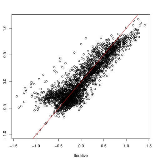
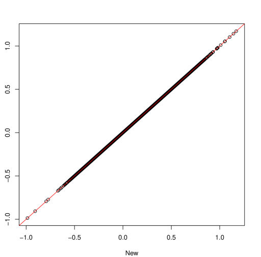
Figure 1: Shapley values for the country variable in the numerical case study. Shapley values for the training data are plotted. We plot the iterative estimates, the estimates from the sequential method and the new method. Along the vertical direction we plot the sequential estimates while along the horizontal we plot the iterative estimates (on the left) and the estimates from the new method (on the right). The red line indicates the line $y=x$.

6 Discussion and conclusion

In Table 1 we show the Shapley values for the first training observation. We have given the variable names shorter names so that we can use one table. From this table we observe close correspondence between the new and sequential methods. The iterative method estimates in some cases the correct Shapley value, while for e.g V13 (GDP per capita), the estimate is quite off. In Figure 1 we have plotted the Shapley values for all training observations for the country variable. We observe good correspondence for the new and sequential methods, while much worse correspondence for the iterative method. In fact, in some cases the true Shapley value is close to 0 while the iterative method says about -1.5, which is not very accurate.

The run-times and above results indicates that we can obtain better Shapley value estimates from the new method than from the iterative estimates and in less (or almost the same amount of) time.

There are also other competing methods not studied here, such as a method in the popular shap package (Lundberg and Lee, 2017), which assumes the variables follows a multivariate Gaussian distribution and also uses sampling. As we have categorical variables in our case study, the assumption is violated.

It should be clear to the reader that the method can easily be extended to accommodate some types of splines, e.g splines from the rms-package (Harrell Jr, 2025). The reason is that the coefficients can be estimated using a linear regression model. This makes our methodology more flexible.

Further enhancements of the method is possible by using parallelization. In shapr one can also perform parallelization, but in our work we compared serial computations against serial computations. A recent method with parallel decompositions of a symmetric positive definite matrix is Fattah et al. (2025), where also existing sparse factorization packages are compared to each other and the new method.

Our method is also cursed with the curse of dimensionality: When $p$ increases, such as $p=30$, the machine eventually runs out of memory. However, there are options to deal with this problem. One option is sampling, as described before. However, instead of using a few hundred of coalitions, as often done, one can now use thousands of coalitions. We have illustrated that model fitting will be fast, indicating that the new method is a major advancement. Another option is to split the model estimation into equal “chunks”, where for instance half of the models is fitted, then the remaining half is fitted and finally the results are combined before estimating the Shapley values.

References

- Aas et al. (2021) Aas, K., M. Jullum, and A. Løland (2021). Explaining individual predictions when features are dependent: More accurate approximations to Shapley values. Artificial Intelligence 298, 103502.
- Bates et al. (2025) Bates, D., M. Maechler, and M. Jagan (2025). Matrix: Sparse and Dense Matrix Classes and Methods. R package version 1.7-3.
- Fattah et al. (2025) Fattah, E. A., H. Ltaief, H. Rue, and D. Keyes (2025). sTiles: An Accelerated Computational Framework for Sparse Factorizations of Structured Matrices. arXiv preprint arXiv: 2501.02483.
- Harrell Jr (2025) Harrell Jr, F. E. (2025). rms: Regression Modeling Strategies. R package version 8.0-0.
- Henderson and Searle (1981) Henderson, H. V. and S. R. Searle (1981). On Deriving the Inverse of a Sum of Matrices. SIAM Review 23(1), 53–60.
- Jullum et al. (2025) Jullum, M., L. H. B. Olsen, J. Lachmann, and A. Redelmeier (2025). shapr: Explaining Machine Learning Models with Conditional Shapley Values in R and Python. arXiv preprint arXiv: 2504.01842.
- Lundberg and Lee (2017) Lundberg, S. M. and S.-I. Lee (2017). A unified approach to interpreting model predictions. In I. Guyon, U. V. Luxburg, S. Bengio, H. Wallach, R. Fergus, S. Vishwanathan, and R. Garnett (Eds.), Advances in Neural Information Processing Systems, Volume 30. Curran Associates, Inc.
- Mayer and Watson (2024) Mayer, M. and D. Watson (2024). kernelshap: Kernel SHAP. R package version 0.7.0.
- Olsen et al. (2024) Olsen, L. H. B., I. K. Glad, M. Jullum, and K. Aas (2024). A comparative study of methods for estimating model-agnostic shapley value explanations. Data Mining and Knowledge Discovery 38(4), 1782–1829.
- R Core Team (2025) R Core Team (2025). R: A Language and Environment for Statistical Computing. Vienna, Austria: R Foundation for Statistical Computing.
- Rue and Held (2005) Rue, H. and L. Held (2005). Gaussian Markov random fields: theory and applications. CRC press.
- Shapley (1953) Shapley, L. S. (1953). Contributions to the Theory of Games, Volume II, Chapter 17. A Value for n-Person Games, pp. 307–318. Princeton University Press.