Recent advances in data-driven methods for degradation modelling across applications

Abstract

Understanding degradation is crucial for ensuring the longevity and performance of materials, systems, and organisms. To illustrate the similarities across applications, this article provides a review of data-based method in materials science, engineering, and medicine. The methods analyzed in this paper include regression analysis, factor analysis, cluster analysis, Markov Chain Monte Carlo, Bayesian statistics, hidden Markov models, nonparametric Bayesian modeling of time series, supervised learning, and deep learning. The review provides an overview of degradation models, referencing books and methods, and includes detailed tables highlighting the applications and insights offered in medicine, power engineering, and material science. It also discusses the classification of methods, emphasizing statistical inference, dynamic prediction, machine learning, and hybrid modeling techniques. Overall, this review enhances understanding of degradation modelling across diverse domains.

scriptsize[table]font=scriptsize

[AGH]organization=AGH University of Krakow, Dept. of Automatic Control & Robotics,addressline=al. Mickiewicza 30, city=Krakow, postcode=30-059, state=Poland, country=corresponding author: jb@agh.edu.pl

[NTNU]organization=NTNU,addressline=Department of Engineering Cybernetics, city=Trondheim, postcode=7034, country=Norway. Currently with DCSC at TU Delft in the Netherlands

1 Introduction

Degradation is defined as a process in which the quality or condition of a material, system, or organism deteriorates over time, leading to a decline in performance or functionality. This process is crucial to understand for technical, engineering, and economical reasons, as it influences the service life of various structures and materials. In this article, we present a summary of existing research on degradation modeling, encompassing a diverse range of approaches across applications in material science, engineering, and medicine.

Degradation modeling plays a crucial role in various fields, including engineering, reliability analysis, and system optimization. Understanding the behavior of degrading systems and predicting their remaining useful life is essential for effective maintenance, resource allocation, and system design. In this review, we will present various statistical methods that have been applied to degradation modeling, exploring both traditional statistical techniques and more advanced approaches, such as machine learning algorithms. By examining these methods, we provide insights into the strengths, limitations, and potential applications of each approach in degradation modeling.

This paper is structured as follows. In Section 2 we introduce the key preliminaries on degradation modeling, including definitions, ISO standards across medicine, engineering and materials science, and the distinction between physical, data‐driven and knowledge‐based approaches. Section 3 surveys the existing literature, summarizing prior review papers and textbook treatments, and presents a comparative analysis of publication trends over time in the three application domains. In Section 4 we propose our classification of data-based methods into three main groups - statistical inference, dynamic prediction and machine learning - and describe each class in detail. Section 5 examines how these methods have been used in material science, power engineering and medicine, highlighting domain-specific preferences and hybrid combinations. Section 6 discusses open challenges and future research directions, such as uncertainty quantification, missing-data handling, data fusion, and scalability. Finally, Section 7 concludes with a summary of the main insights and recommendations for practitioners and researchers.

2 Preliminaries

2.1 Degradation across applications

A typical classification of degradation models discerns among three groups of models: physical models, data-driven models, and knowledge-based models [1]. Physical and knowledge-based models are typically application-specific because they describe particular phenomena occurring in a system. Conversely, data-based models focus on capturing the decline in performance or functionality regardless of the field of application. Despite the diverse applications of degradation, there are similarities in how degradation is described. Thus, similar data-based methods for degradation modelling can be used across disjoint applications. To illustrate the similarities across applications, this article provides a review of data-based method in materials science, engineering, and medicine.

In material science, degradation encompasses the deterioration of physical properties such as strength, ductility, and corrosion resistance of materials [2]. Understanding degradation processes is crucial for selecting materials that can maintain their performance over time, ensuring the reliability and safety of structures and components. This includes various degradation mechanisms, such as fatigue, creep, oxidation, and environmental degradation, which impact the structural integrity and reliability of materials and components.

In engineering, degradation refers to the decline in the performance or reliability of mechanical or electronic systems due to wear, fatigue, or aging [1]. This can include processes such as stress relaxation, thermal degradation, and chemical degradation, which affect the overall performance of materials and structures. Furthermore, the study of degradation in engineering involves the assessment of material degradation under different operational conditions, including temperature, humidity, and mechanical loading, to ensure the long-term functionality and safety of engineering systems.

In medicine, degradation focuses on the decline in the health or function of biological systems, such as tissues, organs, or physiological processes. This encompasses biodegradation and biodeterioration, where the vital activities of organisms lead to undesirable changes in the properties of materials. In addition, the understanding of degradation in medicine extends to biomaterial degradation, including implants corrosion, drug delivery systems degradation, and deterioration of biological tissues, with implications for the efficacy and safety of medical interventions.

Table 1 summarizes the definitions of degradation as outlined in ISO standards across the fields of medicine, engineering, and material science. Each application has specific standards that address the implications and management of degradation in their respective contexts.

Table 1: Definitions of degradation from ISO Standards

Application	Definitions from ISO Standards
Medicine	ISO 10993-13:2010 - the standard outlines methods for identifying and quantifying degradation products from polymeric medical devices, focusing on chemical alterations of the finished device [3].
	ISO 10993-1:2018 - the standard provides a framework for the biological evaluation of medical devices, including considerations for degradation and its impact on biocompatibility [4].
	ISO 14971:2019 - the standard addresses the application of risk management to medical devices, including risks associated with material degradation over time [5].
	ISO 13485:2016 - the standard specifies requirements for a quality management system where an organization needs to demonstrate its ability to provide medical devices that consistently meet customer and regulatory requirements, including those related to degradation [6].
Engineering	ISO 55000:2014 - the standard provides an overview of asset management, including the management of degradation in engineering components to ensure reliability and performance [7].
	ISO 9001:2015 - the standard outlines quality management principles that include monitoring and managing degradation in engineering processes and products [8].
	ISO 14001:2015 - the standard focuses on environmental management systems, which include considerations for material degradation and its environmental impacts [9].
	ISO 50001:2018 - the standard provides a framework for managing energy performance, which includes addressing degradation in materials and systems to improve energy efficiency [10].
Material Science	ISO 15156-1:2015 - the standard provides guidelines for materials used in oil and gas production, addressing degradation mechanisms such as corrosion and their impact on material selection [11].
	ISO 6892-1:2019 - the standard specifies the method for tensile testing of metallic materials, which includes considerations for degradation effects on mechanical properties [12].
	ISO 11469:2000 - the standard provides guidelines for the identification of plastics and their degradation characteristics, focusing on environmental impacts [13].
	ISO 14040:2006 - the standard outlines principles and framework for life cycle assessment, which includes evaluating material degradation throughout the product life cycle [14].

Despite the specific manifestations of degradation in these fields, the common thread lies in understanding the degradation processes, identification of underlying degradation mechanisms, and prediction of future behavior. This shared objective underscores the interdisciplinary nature of degradation analysis and emphasizes the necessity of a cohesive approach to analyzing and modelling degradation.

2.2 Data-based degradation modelling

Mathematical models of degradation can be divided into analytical models, derived from first principles treating degradation as a physical phenomenon, and data-driven models, focused on describing degradation from experimental data [15] without explicit knowledge about the underlying physics [16]. Thus, developing models of degradation often relies on statistical inference to analyze degradation data, infer deterioration patterns, and provide reliability estimates and predictions based on historical data. Statistical inference methods consist in drawing conclusions about population parameters, making predictions, or testing hypotheses based on the estimated model. They often rely on model selection tools, such as the Akaike information criterion [17], or employ model-free techniques that dynamically adapt to the contextual affinities of a process and capture intrinsic characteristics of the observations.

Dynamic prediction methods model the dynamic evolution of degradation processes considering time-dependent changes in degradation mechanisms, and predicting future degradation behavior. This approach enables the assessment of degradation over time and the prediction of future performance based on dynamic changes in degradation mechanisms.

Lastly, the recent rise of machine learning techniques allows capturing intricate degradation patterns, identifying underlying degradation mechanisms, and making precise predictions using extensive and diverse datasets [18]. These approaches facilitate the comprehensive analysis of degradation behavior and the development of predictive models for various degradation processes.

The three approaches are shown in Fig. 1.

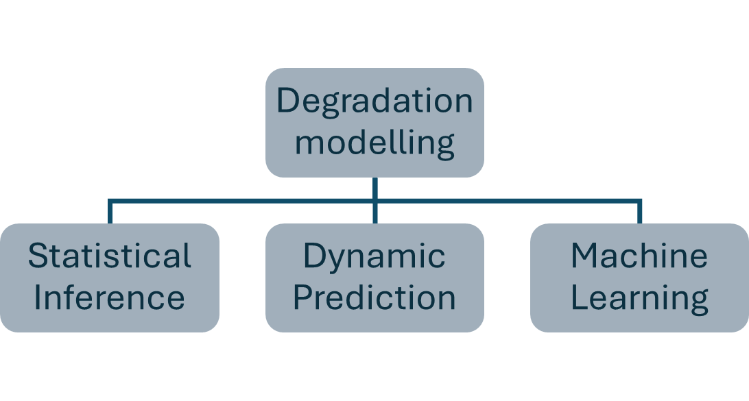
Figure 1: Main approaches to data-based modelling of degradation adopted in this work

3 Background analysis

3.1 Existing reviews of data-based degradation modelling methods

Table 2 provides an overview of methods for degradation modelling from textbooks, emphasizing the methods and proposed applications. The insights derived from these models contribute to the development of effective strategies for system maintenance, optimization, and reliability assessment. In particular, the books emphasize the fact that similar methods are used across applications. For instance, Bayesian modelling is discussed in [19, 20, 21, 22, 23, 24] with application areas from economics and finance, through biostatistics and data analysis, to structural health monitoring.

Table 2: Degradation modelling in textbooks

Ref	Method	Application
[19]	regression analysis, Bayesian statistics	CNC machines
[20]	Markov Chain Monte Carlo, Bayesian statistics	machining tools
[25]	Markov Chain Monte Carlo, hidden Markov models	composite materials
[26]	supervised learning, deep learning	Building materials
[27]	cluster analysis, regression analysis	industrial equipment
[28]	nonparametric Bayesian modeling of time series, Bayesian statistics	infrastructure systems such as bridges or highways
[21]	hidden Markov models, regression analysis	railway track geometry
[22]	Markov Chain Monte Carlo, Bayesian statistics	industrial machinery
[29]	Markov Chain Monte Carlo, supervised learning	brushless direct current motor
[30]	hidden Markov models, nonparametric Bayesian modeling of time series	machinery under different stressors
[31]	Markov Chain Monte Carlo, Bayesian statistics	metal components used in construction
[32]	hidden Markov models, nonparametric Bayesian modeling of time series	concrete structures
[23]	Bayesian statistics, regression analysis	structural components under stress
[24]	nonparametric Bayesian modeling of time series, Markov Chain Monte Carlo	modal properties of structural systems
[33]	Markov Chain Monte Carlo, Bayesian statistics	engineering assets and materials

Table 3 summarizes existing literature reviews on degradation modeling. This compilation shows a broad spectrum of methodologies and classifications within the field of degradation modeling and provides an overview of the various approaches and classifications in the field of degradation modeling.

Table 3: Literature reviews on degradation modeling

Author	Ref	Year	Classification
Firdaus, N., Ab-Samat, H., Prasetyo, B.T.	[34]	2023	defect detection model, Markovian model, machine learning-based predictive model
Jaime-Barquero, E., Bekaert, E., Olarte, J., Zulueta, E., Lopez-Guede, J.M.	[35]	2023	accelerated life testing model, physical-based model, machine Learning-based model
Alimi, O.A., Meyer, E.L., Olayiwola, O.I.	[36]	2022	manual visual assessment model, condition monitoring model, statistical data analysis model
Berghout, T., Benbouzid, M.	[37]	2022	supervised learning model, unsupervised learning model, deep learning model
Zhao, S., Tayyebi, M., Mahdireza Yarigarravesh, Hu, G.	[38]	2023	mechanistic model, stochastic model, statistical model
Xue, K., Yang, J., Yang, M., Wang, D.	[39]	2023	machine learning model, statistical model, data-driven model
Papargyri, L., Theristis, M., Kubicek, B., Papanastasiou, P., Georghiou, G.E.	[40]	2020	statistical model, machine learning model, simulation model
Mondal, M., Kumbhar, G.B.	[41]	2018	neural network-based model, Monte Carlo simulation model, time series forecasting model
Zhang, M., Yang, S.	[42]	2024	support vector clustering model, deep learning model, statistical model
Chakurkar, P.S., Vora, D., Patil, S., Mishra, S., Kotecha, K.	[43]	2023	anomaly detection model, condition monitoring model, time-series analysis model

3.2 Comparative analysis across years

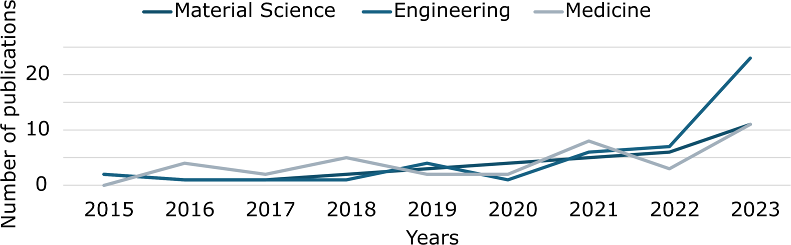
Figure 2: Number of articles over time in the three domains

Figure 2 shows the trends and variations in the numbers of articles across domains and years. In general, we observe an increasing trend in the number of articles over the years for all three domains. The largest increase is observed in Engineering, from two publication in 2015 to 23 publications in 2023. This increase may be explained by increased adoption of computational tools in engineering that allowed use of data-driven methods.

4 Classification with respect to methods

This section presents methods used for degradation modelling. The classification of methods adopted in the paper is shown in Figure 3.

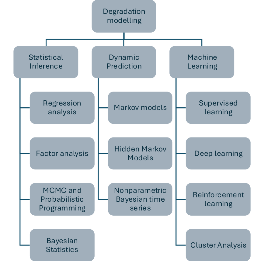
Figure 3: Classification tree of degradation modelling methods, adopted in this paper

4.1 Statistical Inference

Statistical inference models are used to simulate and analyze the processes of tissue and organ degradation in human organisms [44]. These models allow for the analysis of the impact of factors such as aging, injuries, diseases, or the effect of drugs on the degradation of tissues and organs.

Statistical inference models are used to simulate and analyze technological processes in industry [45]. They are employed to forecast the behavior of technological systems, optimize production processes, and identify potential problems.

Statistical inference models are utilized to simulate and analyze various aspects related to the production, transmission, and use of energy [25]. They are used to forecast energy consumption, optimize energy processes, and identify potential areas for energy efficiency improvement.

4.1.1 Regression Analysis

Regression analysis is a fundamental statistical tool for modeling the relationship between a dependent (response) variable and one or more independent (predictor) variables. In its simplest form, the linear regression model can be written as

$$y_{i}=\beta_{0}+\beta_{1}x_{i1}+\cdots+\beta_{p}x_{ip}+\varepsilon_{i},\quad i=1,\dots,n,$$ (1)

where $y_{i}$ denotes the observed response, $x_{ij}$ the value of the $j$th predictor for the $i$th observation, $\beta_{0},\dots,\beta_{p}$ are unknown parameters, and $\varepsilon_{i}$ are random errors, typically assumed to satisfy $\mathbb{E}[\varepsilon_{i}]=0$, $\operatorname{Var}(\varepsilon_{i})=\sigma^{2}$, and $\varepsilon_{i}\perp\!\!\!\perp\varepsilon_{j}$ for $i\neq j$.

Under these assumptions, the ordinary least squares (OLS) estimator for the parameter vector $\boldsymbol{\beta}=(\beta_{0},\beta_{1},\dots,\beta_{p})^{\top}$ is given in matrix form by

$$\widehat{\boldsymbol{\beta}}=\bigl{(}\mathbf{X}^{\top}\mathbf{X}\bigr{)}^{-1}\mathbf{X}^{\top}\mathbf{y},$$ (2)

where $\mathbf{X}\in\mathbb{R}^{n\times(p+1)}$ is the design matrix whose first column is all ones and $\mathbf{y}\in\mathbb{R}^{n}$ the vector of responses. The OLS solution minimizes the residual sum of squares,

$$\widehat{\boldsymbol{\beta}}=\arg\min_{\boldsymbol{\beta}}\,\|\mathbf{y}-\mathbf{X}\boldsymbol{\beta}\|^{2}.$$

Regression analysis allows for hypothesis testing (e.g. $H_{0}\colon\beta_{j}=0$) and confidence interval estimation for coefficients, facilitating interpretability and inference. Extensions include weighted and generalized linear models to accommodate heteroscedasticity or non‐Gaussian responses [46].

Key advantages: simplicity, interpretability, and closed‐form solutions.
Limitations: reliance on linearity, independence, and homoscedasticity assumptions.

Usage: In the power industry, regression analysis precisely describes degradation processes by identifying the relationship between process variables and degradation [47]. This allows for the rapid prediction of degradation based on known process parameters, optimizing maintenance activities.

Regression analysis is also used in medicine to mathematically describe degradation processes in organisms, such as the breakdown of chemicals in tissues [48]. By employing regression analysis, researchers can determine the dynamics of degradation of medicinal substances in patients’ bodies.

4.1.2 Factor Analysis

Factor analysis is a multivariate technique used to explain the covariance structure among a set of observed variables $\mathbf{x}=(x_{1},\dots,x_{p})^{\top}$ in terms of a smaller number of unobserved latent factors $\mathbf{f}=(f_{1},\dots,f_{m})^{\top}$, with $m<p$. The classic common‐factor model is:

$$\mathbf{x}=\boldsymbol{\Lambda}\,\mathbf{f}+\boldsymbol{\varepsilon},$$ (3)

where $\boldsymbol{\Lambda}\in\mathbb{R}^{p\times m}$ is the matrix of factor loadings, and $\boldsymbol{\varepsilon}\sim N(\mathbf{0},\,\boldsymbol{\Psi})$ represents unique variances (specific plus error), with $\boldsymbol{\Psi}$ diagonal. The covariance structure implied by the model is

$$\operatorname{Cov}(\mathbf{x})=\boldsymbol{\Sigma}=\boldsymbol{\Lambda}\boldsymbol{\Lambda}^{\top}+\boldsymbol{\Psi}.$$ (4)

Estimating $\boldsymbol{\Lambda}$ and $\boldsymbol{\Psi}$ can be done via:

• Principal axis factoring, which iteratively estimates communalities $h_{j}^{2}=\sum_{k=1}^{m}\lambda_{jk}^{2}$ and solves eigenvalue problems on the reduced correlation matrix.

• Maximum likelihood (ML), which finds estimates $\widehat{\boldsymbol{\Lambda}},\widehat{\boldsymbol{\Psi}}$ by maximizing the Gaussian log‐likelihood under $H_{0}\colon\boldsymbol{\Sigma}(\boldsymbol{\Lambda},\boldsymbol{\Psi})=\mathbf{S}$, where $\mathbf{S}$ is the sample covariance.

Interpretation hinges on rotated solutions (e.g. varimax) to achieve “simple structure” and on assessing model fit via likelihood‐ratio tests or information criteria.

Key advantages: dimensionality reduction, uncovering latent constructs, and parsimonious modeling.
Limitations: identifiability issues, sensitivity to distributional assumptions, and subjective choice of number of factors [49].

Usage: In engineering processes, factor analysis can be used to identify groups of process variables [50]. They have a significant impact on degradation, leading to a better understanding of the degradation process.

Similarly, in the energy sector, factor analysis is employed to identify significant factors influencing degradation [51]. It helps optimize maintenance activities and improve understanding of degradation processes.

4.1.3 Bayesian Statistics

Bayesian statistics provides a principled framework for learning about unknown parameters $\theta$ by combining prior beliefs $p(\theta)$ with evidence from data $\mathcal{D}$ through the likelihood $p(\mathcal{D}\mid\theta)$. The cornerstone is Bayes’ theorem:

$$p(\theta\mid\mathcal{D})\;=\;\frac{p(\mathcal{D}\mid\theta)\,p(\theta)}{p(\mathcal{D})}\quad\text{where}\quad p(\mathcal{D})=\int p(\mathcal{D}\mid\theta)\,p(\theta)\,d\theta.$$ (5)

The posterior $p(\theta\mid\mathcal{D})$ quantifies updated uncertainty about $\theta$. From it one can derive:

• Point estimates, e.g. the posterior mean $\mathbb{E}[\theta\mid\mathcal{D}]$.

• Credible intervals, defined by $\displaystyle\int_{a}^{b}p(\theta\mid\mathcal{D})\,d\theta=1-\alpha.$

• Posterior predictive distribution for a new observation $\tilde{y}$:

  $$p(\tilde{y}\mid\mathcal{D})\;=\;\int p(\tilde{y}\mid\theta)\,p(\theta\mid\mathcal{D})\,d\theta.$$

Bayesian methods naturally handle hierarchical models by placing priors at multiple levels (e.g. $\theta\sim p(\theta\mid\phi)$, $\phi\sim p(\phi)$), and they explicitly propagate all sources of uncertainty. Computational tools such as Markov Chain Monte Carlo (MCMC) or variational inference allow approximation of posteriors when closed‐form solutions are unavailable [52].

Key advantages: coherent uncertainty quantification, flexible modeling of complex structures, and direct probability statements about parameters.
Limitations: computational intensity, sensitivity to prior choices, and challenges in high‐dimensional settings.

Usage: In the context of dynamic degradation processes of biologically active substances, Bayesian statistics is used to update knowledge based on clinical trial results [53]. This allows for the consideration of the variability of patients’ physiological parameters and their impact on drug degradation.

Bayesian statistics updates knowledge about the degradation of biologically active substances based on clinical trial results [54]. It enhances the modeling of dynamic degradation processes.

4.1.4 Markov Chain Monte Carlo and Probabilistic Programming

Markov Chain Monte Carlo (MCMC) comprises a class of algorithms for generating samples from a target probability distribution $\pi(\theta)$ when direct sampling is infeasible. A key property is that the Markov transition kernel $K(\theta^{\prime}\mid\theta)$ satisfies the detailed balance condition

$$\pi(\theta)\,K(\theta^{\prime}\mid\theta)\;=\;\pi(\theta^{\prime})\,K(\theta\mid\theta^{\prime})\quad\Longrightarrow\quad\int\pi(\theta)\,K(\theta^{\prime}\mid\theta)\,d\theta=\pi(\theta^{\prime}).$$

In the Metropolis–Hastings algorithm, one proposes $\theta^{*}\sim q(\theta^{*}\mid\theta^{(t)})$ and accepts it with probability

$$\alpha=\min\Bigl{(}1,\;\frac{\pi(\theta^{*})\,q(\theta^{(t)}\mid\theta^{*})}{\pi(\theta^{(t)})\,q(\theta^{*}\mid\theta^{(t)})}\Bigr{)},$$

otherwise setting $\theta^{(t+1)}=\theta^{(t)}$. A special case is the Gibbs sampler, which updates each component $\theta_{i}$ by drawing from its full conditional $\pi(\theta_{i}\mid\theta_{-i})$.

Hamiltonian Monte Carlo (HMC) augments the parameter space with auxiliary momentum variables $p\in\mathbb{R}^{d}$ and uses simulated Hamiltonian dynamics to propose distant states with high acceptance probability [55]. One defines the Hamiltonian

$$H(\theta,p)=U(\theta)+K(p)=-\log\pi(\theta)+\tfrac{1}{2}\,p^{\top}M^{-1}p,$$

where $M$ is a mass matrix. Trajectories are simulated via the leapfrog integrator:

$$p\Bigl{(}t+\tfrac{\epsilon}{2}\Bigr{)} =p(t)-\tfrac{\epsilon}{2}\,\nabla_{\theta}U\bigl{(}\theta(t)\bigr{)},$$

$$\theta(t+\epsilon) =\theta(t)+\epsilon\,M^{-1}p\Bigl{(}t+\tfrac{\epsilon}{2}\Bigr{)},$$

$$p(t+\epsilon) =p\Bigl{(}t+\tfrac{\epsilon}{2}\Bigr{)}-\tfrac{\epsilon}{2}\,\nabla_{\theta}U\bigl{(}\theta(t+\epsilon)\bigr{)}.$$

After $L$ steps, the proposal $(\theta^{*},p^{*})$ is accepted with probability $\min\{1,\exp(-\Delta H)\}$.

Probabilistic programming languages (PPLs) such as Stan or BUGS allow users to specify complex hierarchical or latent‐variable models in high‐level syntax; the PPL runtime then automatically constructs and runs efficient MCMC chains (including HMC) to approximate posterior distributions of all parameters.

Key advantages: flexibility to model arbitrary posteriors, efficient exploration in high dimensions (HMC), and automatic uncertainty quantification.
Limitations: convergence diagnostics required, choice of integrator step‐size and path length in HMC, and potentially high computational cost.

Usage: In the context of variable energy conditions, MCMC accounts for uncertainties in modeling the degradation of biologically active substances [21]. It enables effective prediction of future degradation states based on previous observations.

MCMC efficiently samples complex probability distributions, which is crucial in modeling step degradation [56]. It facilitates effective prediction of future degradation states based on previous observations.

4.2 Dynamic Prediction

In material science, Markov models enable engineers to analyze temporal dependencies and transitions between different states in a process. This allows for the prediction of future states, identification of bottlenecks, and optimization of process parameters for improved efficiency and productivity. Hidden Markov Models can uncover hidden patterns and detect anomalies in processes, aiding in process control and optimization.

In power engineering, dynamic prediction methods play a vital role in forecasting electricity demand, optimizing power generation, and managing energy resources. Markov models can accurately forecast short-term and long-term load demand by modeling the temporal dependencies and transitions in power consumption patterns. Hidden Markov Models help identify hidden states and patterns in power generation and consumption, facilitating efficient energy management and resource allocation. Nonparametric Bayesian time series modeling considers factors such as weather conditions and time of day to predict electricity demand accurately.

In medicine, dynamic prediction methods have significant applications, ranging from disease prognosis to treatment optimization. Markov models can model disease progression and predict patient outcomes based on current health states. Hidden Markov Models are valuable for modeling latent variables and hidden dynamics in medical data, enabling early detection of diseases and personalized treatment strategies. Nonparametric Bayesian time series modeling captures the complex temporal dynamics of patient data, facilitating accurate predictions of disease progression, treatment response, and prognosis.

4.2.1 Markov models

Markov models are useful for modeling abrupt degradation by considering the nonlinear relationships between process variables and degradation [23]. They enable the forecasting of future degradation states based on previous observations and can incorporate dynamic changes in the degradation process.

A (discrete‐time) Markov model represents the evolution of a system through a finite (or countable) set of states $\mathcal{S}=\{1,\dots,K\}$, where the probability of a transition depends only on the current state. If $X_{t}\in\mathcal{S}$ denotes the state at time $t$, the Markov property is

$$\Pr\bigl{(}X_{t+1}=j\mid X_{t}=i,\,X_{t-1},\dots,X_{0}\bigr{)}\;=\;\Pr\bigl{(}X_{t+1}=j\mid X_{t}=i\bigr{)}=:p_{ij},\quad i,j\in\mathcal{S}.$$ (6)

The one‐step transition probabilities $p_{ij}$ form the transition matrix $P=(p_{ij})$, satisfying $\sum_{j}p_{ij}=1$ for each $i$. The $n$‐step transition probabilities are given by the Chapman–Kolmogorov equations,

$$p_{ij}^{(n)}\;=\;\Pr(X_{t+n}=j\mid X_{t}=i)\;=\;\bigl{(}P^{n}\bigr{)}_{ij},\quad P^{n}=\underbrace{P\cdots P}_{n\text{ times}}.$$ (7)

If $\boldsymbol{\pi}^{(t)}$ is the row vector of state‐probabilities at time $t$, then

$$\boldsymbol{\pi}^{(t+n)}\;=\;\boldsymbol{\pi}^{(t)}\,P^{n}.$$

For ergodic chains (irreducible and aperiodic), there exists a unique stationary distribution $\boldsymbol{\pi}^{*}$ satisfying $\boldsymbol{\pi}^{*}=\boldsymbol{\pi}^{*}\,P$; this can be used for long‐term degradation prediction. In absorbing chains, mean time to absorption and absorption probabilities provide estimates of remaining useful life.

Key advantages: simple formulation, closed‐form $n$‐step predictions, and well‐studied theory of long‐run behavior.
Limitations: state‐space discretization may be coarse, and the loss of history beyond the current state may oversimplify gradual degradation [57].

Usage: In the context of discontinuous energy processes, Markov models are important for modeling abrupt degradation and considering dynamic changes in the degradation process, especially under changing energy conditions [58]. They also allow for the inclusion of nonlinear relationships between process variables and degradation.

In medicine, Markov models can be used to model changes in patients’ health status, predict the course of diseases, and assess the risk of drug degradation [59]. They consider the dynamic changes in patients’ bodies and their impact on drug degradation.

4.2.2 Hidden Markov Models

Hidden Markov Models are used to model abrupt degradation by considering the nonlinear relationships between process variables and degradation [60]. They enable the forecasting of future degradation states based on previous observations.

A Hidden Markov Model (HMM) describes a system where an unobserved (hidden) state sequence $\{X_{t}\}$ evolves as a Markov chain over states $\mathcal{S}=\{1,\dots,K\}$, and at each time $t$ emits an observation $Y_{t}$ according to a state‐dependent distribution. An HMM is specified by:

• Initial distribution $\pi_{i}=\Pr(X_{1}=i)$.

• Transition matrix $A=(a_{ij})$ with $a_{ij}=\Pr(X_{t+1}=j\mid X_{t}=i)$.

• Emission probabilities $b_{i}(y)=\Pr(Y_{t}=y\mid X_{t}=i)$ (or density $b_{i}(y)$ for continuous $Y_{t}$).

The joint probability of a state sequence $\mathbf{x}=(x_{1},\dots,x_{T})$ and observations $\mathbf{y}=(y_{1},\dots,y_{T})$ is

$$\Pr(\mathbf{x},\mathbf{y})=\pi_{x_{1}}\,b_{x_{1}}(y_{1})\,\prod_{t=2}^{T}a_{x_{t-1},x_{t}}\,b_{x_{t}}(y_{t}).$$

Key computations include:

1. Filtering / likelihood: via the forward recursion $\alpha_{t}(j)=\bigl{[}\sum_{i}\alpha_{t-1}(i)a_{ij}\bigr{]}\,b_{j}(y_{t})$.

2. Decoding: the Viterbi algorithm finds $\arg\max_{\mathbf{x}}\Pr(\mathbf{x}\mid\mathbf{y})$.

3. Learning: Baum–Welch (EM) updates $\pi,A,b$ by maximizing the data likelihood.

HMMs capture abrupt or regime‐switching degradation by modeling latent condition changes and corresponding observation patterns.

Key advantages: ability to model unobserved regimes, efficient inference via dynamic programming.
Limitations: choice of state‐space size, assumption of conditional independence of observations [61].

Usage: In the context of discontinuous energy processes, Hidden Markov Models are important for modeling abrupt degradation [62]. It helps consider dynamic changes in the degradation process, especially under changing energy conditions.

Hidden Markov Models can be effectively used in medicine to model changes in patients’ health, taking into account dynamic fluctuations in patients’ bodies and their impact on drug degradation [63]. These advanced models allow for predicting the effectiveness of therapies.

4.2.3 Nonparametric Bayesian Time Series Modeling

Nonparametric Bayesian methods allow the model complexity to grow with data by placing priors on infinite‐dimensional objects. Three widely used approaches in time series are:

Dirichlet Process Mixtures

Partition the series $\{y_{t}\}_{t=1}^{T}$ into an unknown number of regimes, indexed by latent parameters $\{\theta_{k}\}$. A Dirichlet Process (DP) prior on the mixing measure $G$ induces a countably infinite mixture:

$$G \sim\mathrm{DP}(\alpha,G_{0}),$$

$$\theta_{t}\mid G \sim G,\quad y_{t}\mid\theta_{t}\;\sim\;F\bigl{(}y_{t}\mid\theta_{t}\bigr{)}.$$ (8)

Using the stick‐breaking construction,

$$G=\sum_{k=1}^{\infty}\pi_{k}\,\delta_{\theta_{k}},\quad\pi_{k}=\beta_{k}\prod_{l<k}(1-\beta_{l}),\quad\beta_{k}\sim\mathrm{Beta}(1,\alpha),$$

one obtains an adaptive mixture that clusters observations into regimes with similar dynamics. Posterior inference (e.g. via Gibbs sampling) estimates both the number of regimes and their parameters.

Gaussian Process Regression

Model the latent signal $f\colon t\mapsto\mathbb{R}$ as a Gaussian Process (GP):

$$f(t) \sim\mathcal{GP}\bigl{(}m(t),\,k(t,t^{\prime})\bigr{)},$$

$$y_{t} =f(t)+\varepsilon_{t},\quad\varepsilon_{t}\sim N(0,\sigma^{2}).$$ (9)

The kernel $k(t,t^{\prime})$ encodes smoothness or periodicity, and the GP posterior provides closed‐form predictive distributions:

$$f_{*}\mid\mathbf{y}\;\sim\;N\bigl{(}K_{*}K^{-1}\mathbf{y},\;K_{**}-K_{*}K^{-1}K_{*}^{\top}\bigr{)},$$

where $K=[k(t_{i},t_{j})]$, $K_{*}=[k(t_{*},t_{j})]$, etc.

Prophet

Prophet is an additive forecasting model designed for business time series, decomposing $y_{t}$ into trend $g(t)$, seasonality $s(t)$, holiday effects $h(t)$, and noise:

$$y_{t}=g(t)+s(t)+h(t)+\varepsilon_{t},\quad\varepsilon_{t}\sim N(0,\sigma^{2}).$$ (10)

The trend $g(t)$ is modeled as a piecewise linear (or logistic) function with automatic changepoint detection:

$$g(t)=\bigl{(}k+a(t)^{\top}\boldsymbol{\delta}\bigr{)}\,t+\bigl{(}m+a(t)^{\top}\boldsymbol{\gamma}\bigr{)},$$

where $a(t)$ indicates segments, $k,m$ are base rate and offset, and $\boldsymbol{\delta},\boldsymbol{\gamma}$ are adjustments at changepoints. Seasonality $s(t)$ uses Fourier series:

$$s(t)=\sum_{n=1}^{N}\Bigl{[}\alpha_{n}\cos\bigl{(}2\pi nt/P\bigr{)}+\beta_{n}\sin\bigl{(}2\pi nt/P\bigr{)}\Bigr{]},$$

and $h(t)$ includes user‐specified events. Prophet is fitted via MAP estimation with weakly informative priors, yielding fast, interpretable forecasts [64].

Key advantages: automatic changepoint detection, interpretable components, and scalability to large datasets.
Limitations: assumes additive structure, may struggle with highly irregular dynamics, and limited probabilistic uncertainty beyond the MAP fit.

4.3 Machine Learning

Machine learning methods enable automatic detection of patterns in process data and building predictive models based on them [65]. They facilitate adaptive degradation modeling, allowing for the modeling of degradation in engineering processes using a wide range of predictive algorithms.

In the power industry, machine learning methods enable adaptive modeling of degradation [66]. It may consider changing process conditions and optimizing maintenance operations.

In medicine, machine learning methods can be used to predictively model drug degradation based on clinical and laboratory data [27]. They enable adaptive modeling of drug degradation, automatic detection of drug degradation patterns, and optimization of therapeutic doses.

4.3.1 Supervised Learning

Supervised learning aims to learn a mapping $f:\mathcal{X}\to\mathcal{Y}$ from input–output pairs $\mathcal{D}=\{(x_{i},y_{i})\}_{i=1}^{n}$, where each $y_{i}$ is a known label or response. The model $f(x;\theta)$, parameterized by $\theta$, is trained by minimizing an empirical risk functional:

$$\widehat{\theta}\;=\;\arg\min_{\theta}\;\frac{1}{n}\sum_{i=1}^{n}\ell\bigl{(}y_{i},\,f(x_{i};\theta)\bigr{)}$$ (11)

where $\ell(\cdot,\cdot)$ is a loss function (e.g. squared error $\ell(y,\hat{y})=(y-\hat{y})^{2}$ for regression or cross‐entropy $\ell(y,\hat{y})=-\sum_{k}y_{k}\log\hat{y}_{k}$ for classification).

Two primary supervised tasks are:

• Regression: $\mathcal{Y}=\mathbb{R}$, predicting continuous degradation measures (e.g. wear rate).

• Classification: $\mathcal{Y}=\{1,\dots,C\}$, labeling discrete states (e.g. “healthy” vs. “faulty”).

Common algorithmic frameworks include linear models, support vector machines, decision trees and ensembles, and feed‐forward neural networks. Model selection and regularization (e.g. ridge, lasso) control complexity and mitigate overfitting.

Key advantages: direct use of labeled data, flexibility across tasks, and mature theory for generalization (e.g. VC‐dimension, Rademacher complexity).
Limitations: requires substantial labeled data, sensitive to label noise, and potential overfitting without proper regularization [67].

Usage: In the power industry, supervised learning methods enable adaptive modeling of degradation [68]. It considers changing process conditions, and optimizing maintenance operations.

In medicine, supervised learning allows for adaptive modeling of drug degradation based on individual patient characteristics [69]. It may optimize therapeutic doses and assessing degradation risk.

4.3.2 Deep Learning

Deep learning refers to a class of machine learning methods based on artificial neural networks with multiple hidden layers, which can automatically learn hierarchical feature representations from raw data. A feed‐forward deep neural network with $L$ layers can be defined recursively as

$$\mathbf{a}^{(0)} =\mathbf{x},$$

$$\mathbf{z}^{(l)} =W^{(l)}\mathbf{a}^{(l-1)}+\mathbf{b}^{(l)},\quad l=1,\dots,L,$$

$$\mathbf{a}^{(l)} =\phi\bigl{(}\mathbf{z}^{(l)}\bigr{)},$$ (12)

where $\mathbf{x}\in\mathbb{R}^{d}$ is the input, $W^{(l)}$ and $\mathbf{b}^{(l)}$ are the weights and biases of layer $l$, and $\phi(\cdot)$ is a nonlinear activation (e.g. ReLU, sigmoid). The network’s output $\hat{\mathbf{y}}=\mathbf{a}^{(L)}$ is compared to the true label $\mathbf{y}$ via a loss function $\ell(\mathbf{y},\hat{\mathbf{y}})$, and parameters are optimized by backpropagation and stochastic gradient descent:

$$\theta\leftarrow\theta-\eta\,\nabla_{\theta}\frac{1}{n}\sum_{i=1}^{n}\ell\bigl{(}\mathbf{y}_{i},\,\hat{\mathbf{y}}_{i}\bigr{)}.$$

Extensions include convolutional neural networks (CNNs) for spatial degradation patterns and recurrent architectures (RNNs / LSTMs) for temporal degradation sequences. Deep models excel at capturing complex, nonlinear relationships in high‐dimensional sensor or image data, which is critical for accurate degradation prediction and anomaly detection.

Key advantages: automatic feature learning, state‐of‐the‐art predictive performance in large datasets, and flexible architectures for diverse data modalities.
Limitations: large data and computational requirements, potential overfitting, and reduced interpretability of learned features [70].

Usage: In the field of power engineering, deep learning facilitates advanced pattern recognition in modeling degradation and predicting energy processes [26]. It enables adaptive modeling of degradation risk in energy processes.

In medicine, deep learning enables advanced recognition of drug degradation patterns [51]. It contributes to adaptive modeling, prediction of therapy efficacy, and assessment of degradation risk.

4.3.3 Reinforcement Learning

Reinforcement learning (RL) addresses sequential decision–making under uncertainty by learning a policy $\pi(a\mid s)$ that maximizes expected cumulative reward in a Markov decision process (MDP). An MDP is defined by the tuple $(\mathcal{S},\mathcal{A},P,r,\gamma)$ where:

• $\mathcal{S}$ is the state space, $\mathcal{A}$ the action space.

• $P(s^{\prime}\mid s,a)$ is the transition probability.

• $r(s,a)$ is the immediate reward.

• $\gamma\in[0,1)$ is the discount factor.

The goal is to maximize the return $G_{t}=\sum_{k=0}^{\infty}\gamma^{k}\,r(s_{t+k},a_{t+k})$. The state‐value and action‐value functions under policy $\pi$ satisfy the Bellman equations:

$$V^{\pi}(s) =\mathbb{E}_{\pi}\bigl{[}G_{t}\mid s_{t}=s\bigr{]}=\sum_{a}\pi(a\mid s)\Bigl{[}r(s,a)+\gamma\sum_{s^{\prime}}P(s^{\prime}\mid s,a)V^{\pi}(s^{\prime})\Bigr{]},$$ (13)

$$Q^{\pi}(s,a) =r(s,a)+\gamma\sum_{s^{\prime}}P(s^{\prime}\mid s,a)\sum_{a^{\prime}}\pi(a^{\prime}\mid s^{\prime})\,Q^{\pi}(s^{\prime},a^{\prime}).$$ (14)

Model‐free methods include:

• Q‐learning (off‐policy): $\displaystyle Q_{t+1}(s_{t},a_{t})\leftarrow Q_{t}(s_{t},a_{t})+\alpha\bigl{[}r_{t}+\gamma\max_{a^{\prime}}Q_{t}(s_{t+1},a^{\prime})-Q_{t}(s_{t},a_{t})\bigr{]}.$

• Policy gradient (on‐policy): optimize $J(\theta)=\mathbb{E}_{\pi_{\theta}}[G_{t}]$ via $\nabla_{\theta}J=\mathbb{E}_{\pi_{\theta}}\bigl{[}\nabla_{\theta}\log\pi_{\theta}(a\mid s)\,Q^{\pi_{\theta}}(s,a)\bigr{]}.$

Deep RL integrates neural networks to approximate $Q$ or $\pi$ (e.g. DQN, actor–critic). In degradation modeling, RL can learn maintenance or control policies that dynamically trade off immediate performance versus long‐term system health.

Key advantages: learns adaptive policies without explicit system models; handles stochastic, nonstationary environments.
Limitations: sample‐inefficient; high variance in gradient estimates; requires careful tuning of hyperparameters [71].

Usage: In the field of power engineering, reinforcement learning is used for adaptive degradation modeling [72]. It considers dynamic changes in the degradation process, especially under changing energy conditions.

In medicine, reinforcement learning is employed for adaptive modeling of drug degradation [73]. It enables the prediction of therapy effectiveness and the assessment of degradation risk.

4.3.4 Cluster Analysis

Cluster analysis is an unsupervised learning technique that seeks to partition a set of $n$ observations $\{x_{i}\in\mathbb{R}^{d}\}_{i=1}^{n}$ into $K$ groups (clusters) $\{C_{k}\}_{k=1}^{K}$ such that observations within the same cluster are more similar to each other than to those in other clusters. Two common approaches are:

K‐Means Clustering

Assign each $x_{i}$ to the cluster with the nearest centroid $\mu_{k}$, by minimizing the within‐cluster sum of squares (WCSS):

$$\{\widehat{C}_{k},\widehat{\mu}_{k}\}_{k=1}^{K}=\arg\min_{\{C_{k},\mu_{k}\}}\;\sum_{k=1}^{K}\sum_{x_{i}\in C_{k}}\|x_{i}-\mu_{k}\|^{2}.$$ (15)

The standard algorithm alternates between (i) assignment: $C_{k}\leftarrow\{\,i:\|x_{i}-\mu_{k}\|\leq\|x_{i}-\mu_{j}\|\;\forall j\}$, and (ii) update: $\mu_{k}\leftarrow\tfrac{1}{|C_{k}|}\sum_{x_{i}\in C_{k}}x_{i}$, until convergence.

Hierarchical Clustering

Builds a tree (dendrogram) of clusters either by agglomeration (bottom‐up) or division (top‐down). In agglomerative clustering, start with each point as its own cluster and at each step merge the pair $(C_{a},C_{b})$ minimizing a linkage criterion, e.g.

$$d_{\text{single}}(C_{a},C_{b})=\min_{x_{i}\in C_{a},x_{j}\in C_{b}}\|x_{i}-x_{j}\|,\quad d_{\text{complete}}(C_{a},C_{b})=\max_{x_{i}\in C_{a},x_{j}\in C_{b}}\|x_{i}-x_{j}\|.$$

By cutting the dendrogram at a chosen height, one obtains a desired number of clusters.

Key advantages: no need for labeled data; can discover unknown structure; interpretable via centroids or dendrograms.
Limitations: choice of $K$ or cut‐height is subjective; sensitive to scaling and noise; may find only spherical clusters (for K‐means) or be computationally expensive ($\mathcal{O}(n^{3})$ for naive hierarchical implementations) [74].

Usage: In the power industry, cluster analysis helps reduce data complexity by identifying important factors influencing degradation processes [75]. It enables mathematical modeling of various degradation cases, contributing to a better understanding of degradation processes.

Cluster analysis is also used in medicine to group degradation events based on similarities in their characteristics [48]. It helps identify groups of process variables that significantly impact the degradation of chemicals in organisms.

5 Classification of methods and their usage across applications

This section presents degradation modeling across domains such as Material Science, Engineering, and Medicine. In Table 4, we provide a comprehensive overview of the number of articles published in each domain, categorized by the methods employed. This analysis reveals the distribution of research efforts across the three domains, highlighting how each method contributes to the understanding and application of degradation modeling.

Table 4: Method used for degradation modelling with dynamic prediction

Method	Material Science	Engineering	Medicine
Statistical inference	25	41	34
Dynamic prediction	21	36	28
Machine learning	23	31	27

5.1 Individual methods

Figure 4(c) provides an overview of the utilization of different techniques in the fields of material science, engineering, and medicine. It encompasses three main categories: statistical inference, dynamic prediction methods, and machine learning.

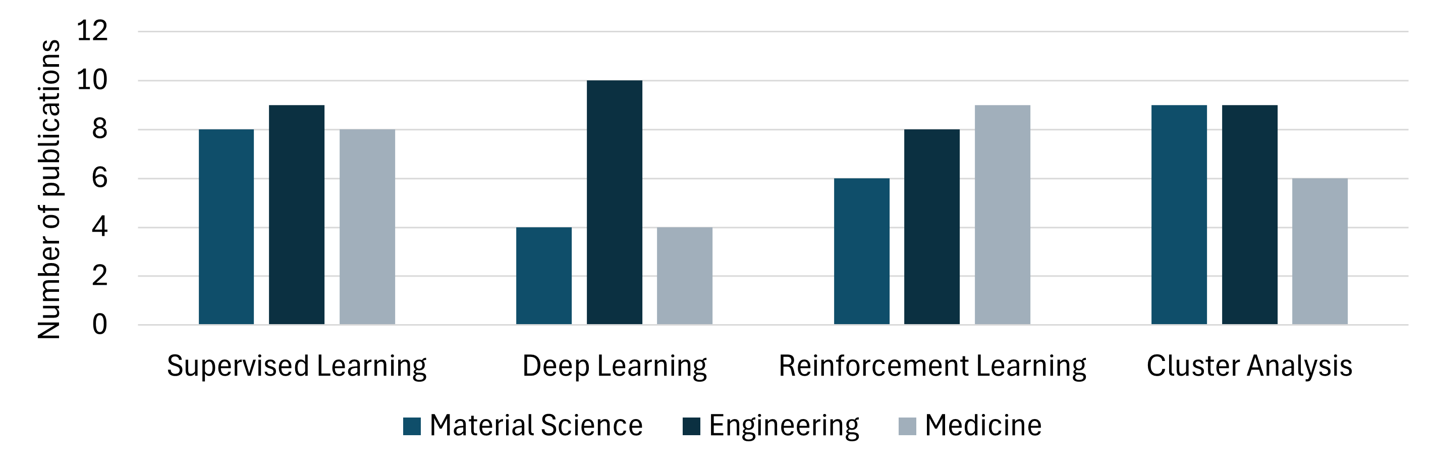
(a) Machine learning

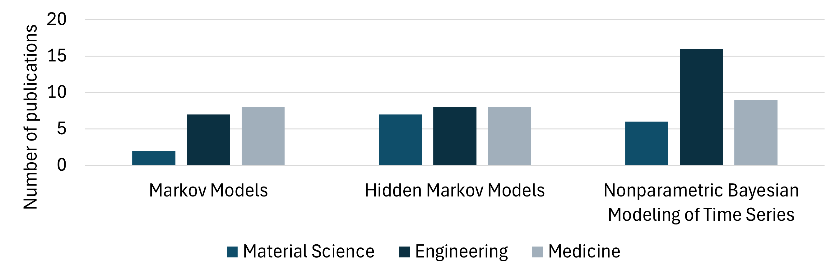
(b) Deep Learning

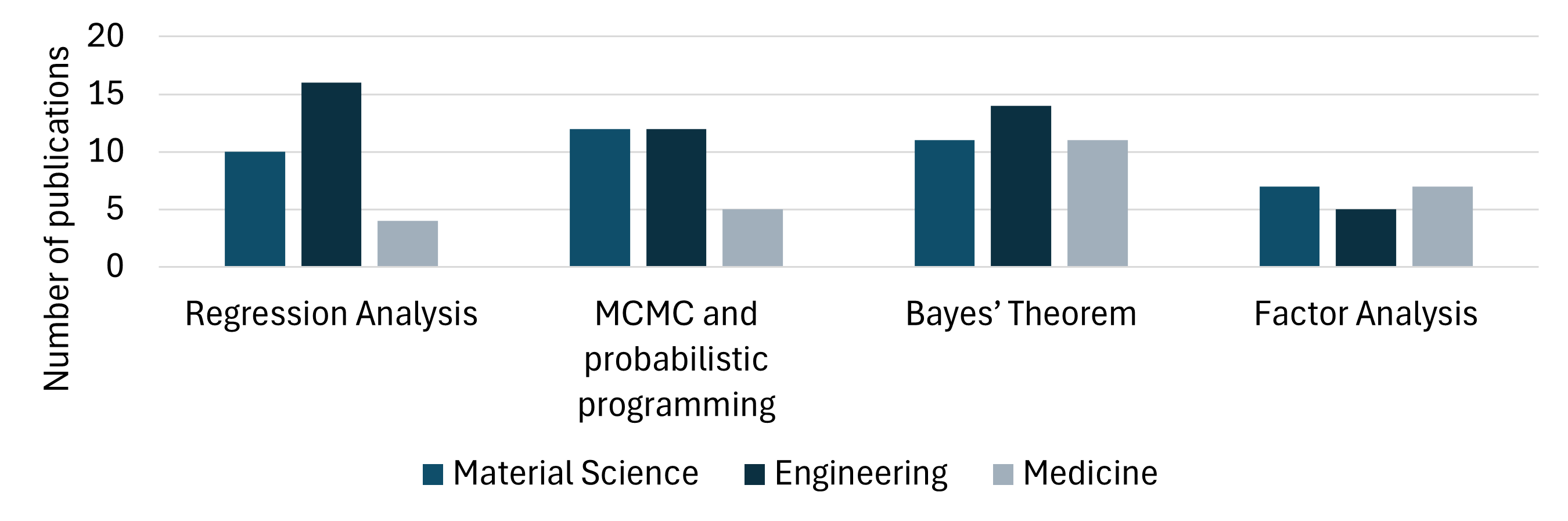
(c) Statistical Inference

Figure 4: Usage of techniques

5.1.1 Statistical inference usage

Table 5 shows the use of techniques from the statistical inference method in three disciplines: material science, power engineering, and medicine.

Markov Chain Monte Carlo (MCMC) + probabilistic programming is applicable in all three disciplines: Material Science, Engineering, and Medicine. This technique is used for sampling from probability distributions and approximating the desired distribution. Regression Analysis is more applicable in Engineering compared to Material Science and Medicine. It is a statistical technique used to model the relationship between variables and make predictions. Bayesian statistics is applicable in all three disciplines, with higher relevance in Medicine. It is a fundamental concept in Bayesian inference and has applications in probabilistic modeling. Factor Analysis has similar relevance in Material Science and Medicine, while being less applicable in Engineering. It is a statistical technique used to explore relationships among observed variables and identify underlying factors.

Table 5 presents a compilation of articles related to degradation models with statistical inference in the field of Material Science. These articles explore various techniques used to study the degradation of materials and provide insights into their behavior under different conditions.

Table 5: Method used for degradation modelling with statistical inference

Method	Material Science	Engineering	Medicine
Regression Analysis	[76, 77, 78, 79, 80, 81, 82, 83, 84, 85]	[86, 87, 88, 89, 90, 91, 92, 93, 94, 95, 96, 97, 98, 99, 100, 101]	[102, 103, 104, 105]
Factor Analysis	[106, 107, 108, 109, 110, 111, 112]	[113, 114, 115, 116, 117]	[118, 119, 120, 121, 122, 123, 124]
Markov Chain Monte Carlo + probabilistic programming	[125, 126, 84, 127, 128, 129, 130, 131, 112, 132, 133, 134]	[135, 136, 137, 138, 139, 140, 141, 142, 114, 143, 144, 97]	[145, 146, 147, 148, 149]
Bayesian statistics	[150, 151, 152, 153, 81, 154, 155, 156, 109, 157, 158]	[159, 160, 161, 95, 162, 163, 164, 165, 166, 167, 168, 169, 170, 171, 172]	[119, 120, 102, 122, 173, 174, 175, 176, 177, 178, 179]

5.1.2 Dynamic prediction usage

Table 6 refers to the number of applications of individual techniques from the dynamic prediction methods method in each of the disciplines, which allows us to conclude the preferences and popularity of particular techniques in particular fields.

Markov Models and Hidden Markov Models are applicable in all three disciplines: Material Science, Engineering, and Medicine. These models are used to analyze and model sequential data with hidden states. Nonparametric Bayesian Modeling of Time Series is more applicable in Engineering compared to Material Science and Medicine. This approach allows for flexible modeling of time series data without making strong assumptions about the underlying distribution. The relevance of these techniques varies across disciplines. For example, Medicine shows higher relevance for Markov Models and Hidden Markov Models compared to Material Science and Engineering. This suggests that these techniques have specific applications or importance in the medical field.

Table 6: Method used for degradation modelling with Dynamic Prediction

Method	Material Science	Engineering	Medicine
Markov models	[133, 180]	[181, 182, 143, 144, 135, 183, 172]	[184, 185, 186, 147, 173, 187, 176, 188]
Hidden Markov Models	[125, 189, 190, 107, 191, 151, 111]	[164, 165, 192, 138, 96, 193, 194, 195]	[175, 196, 186, 177, 197, 104, 179, 198]
Nonparametric Bayesian Time Series Modeling	[128, 129, 130, 108, 131, 132]	[142, 199, 162, 166, 113, 181, 91, 92, 94, 200, 201, 115, 98, 116, 117, 141]	[202, 203, 204, 205, 149, 145, 206, 123, 124]

5.1.3 Machine Learning usage

Table 7 shows the use of different machine learning techniques in three disciplines: material science, power engineering, and medicine.

Table 7 showcases articles in the field of Medicine that focus on specific techniques used in degradation models with statistical inference. Degradation models play a significant role in understanding disease progression, treatment effectiveness, and the performance of medical devices. The articles listed in Table 7 cover a wide range of medical applications, including drug delivery systems, implantable devices, and disease prognosis. By applying statistical inference techniques to degradation data, researchers gain valuable insights into the effectiveness of treatments, the longevity of medical devices, and the progression of diseases.

Table 7: Method used for degradation modelling with machine learning

Method	Material Science	Engineering	Medicine
Supervised Learning	[76, 78, 79, 80, 190, 153, 134, 126]	[89, 90, 193, 168, 93, 207, 195, 208, 100]	[174, 121, 202, 178, 204, 209, 205, 198]
Deep Learning	[77, 210, 82, 152]	[159, 161, 208, 86, 211, 137, 182, 169, 199, 170]	[196, 197, 212, 146]
Reinforcement Learning	[127, 150, 83, 189, 110, 85]	[136, 167, 139, 140, 171, 99, 194, 160]	[213, 184, 214, 215, 118, 103, 203, 216, 187]
Cluster analysis	[106, 210, 191, 154, 155, 156, 157, 158, 180]	[101, 183, 192, 200, 217, 218, 87, 163, 88]	[214, 188, 148, 212, 216, 209]

Supervised Learning is applicable in Material Science, Engineering, and Medicine. It involves training a model using labeled data to make predictions or classify new data points. Deep Learning is more applicable in Engineering compared to Material Science and Medicine. It is a subset of machine learning that focuses on training deep neural networks to learn hierarchical representations of data. Reinforcement Learning is applicable in Engineering and Medicine, with higher relevance in Medicine. It involves training an agent to make decisions in an environment to maximize a reward signal. Cluster Analysis is more applicable in Material Science compared to Engineering and Medicine. It is an unsupervised learning technique used to group similar data points together based on their inherent characteristics.

5.2 Hybrid methods

5.2.1 Statistical Inference and Dynamic Prediction

Figure 5 presents combinations of methods from statistical inference and dynamic prediction. It demonstrates the usage of MCMC in material science, power engineering, and medicine for parameter estimation, exploring distributions, and Bayesian models. MCMC simulations are valuable for simulating complex systems and addressing uncertainty in diverse domains. Nonparametric Bayesian modeling is important in material science, while in power engineering and medicine, MCMC is used for uncertainty quantification and computational modeling.

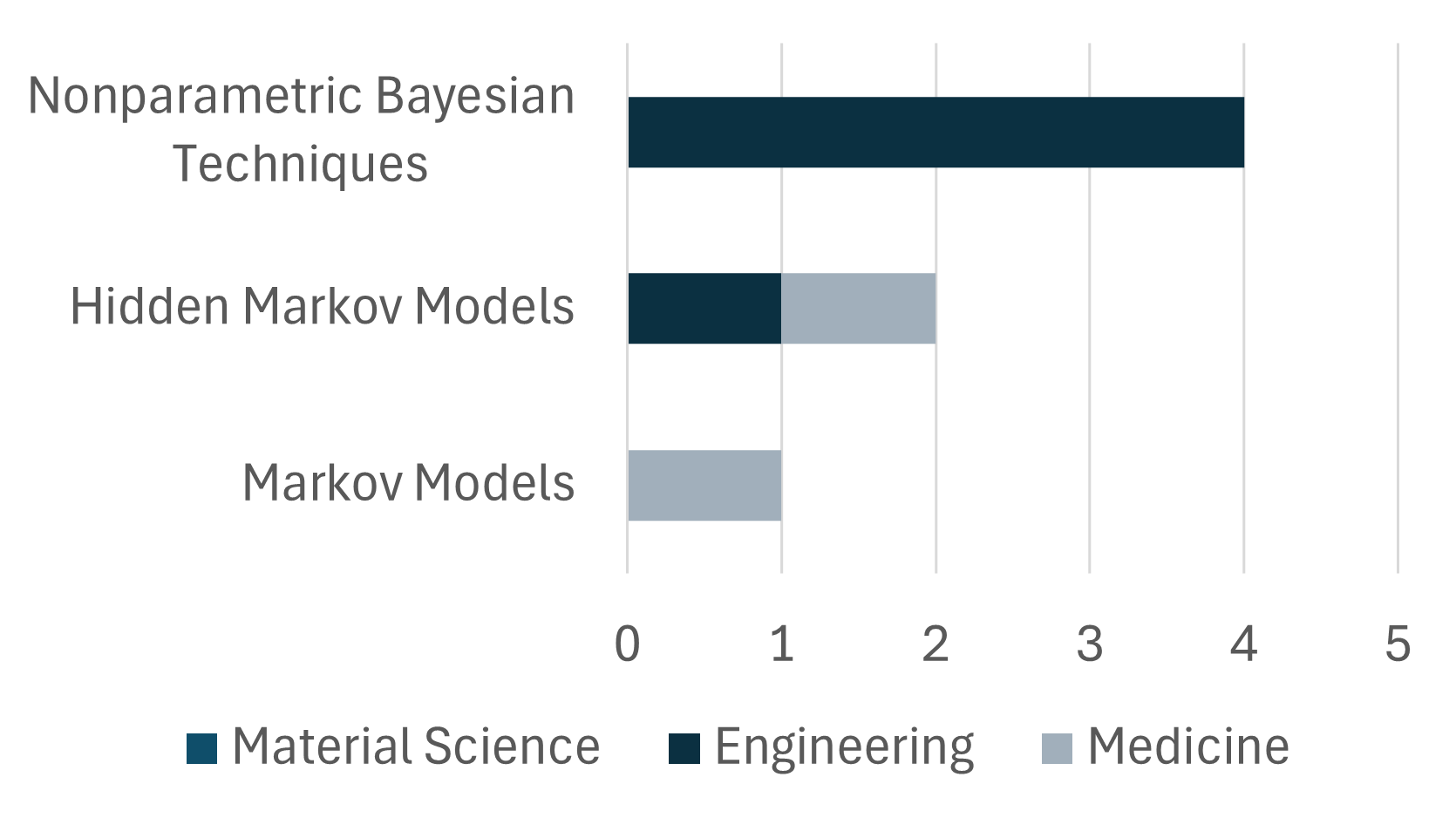
(a) Regression Analysis

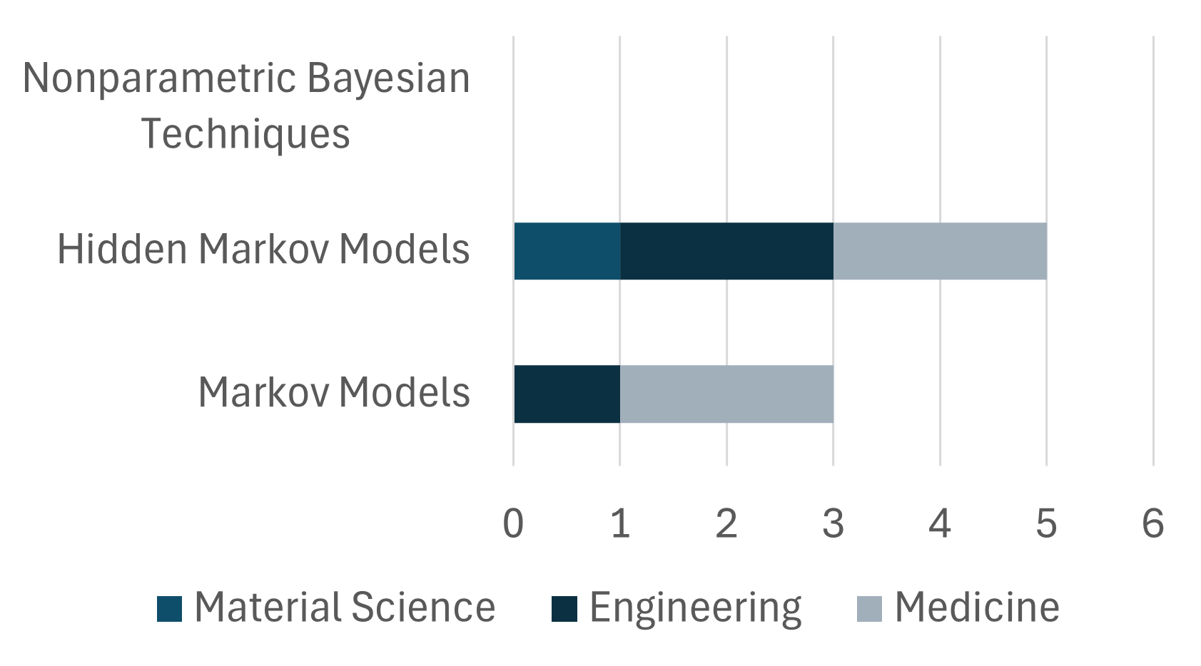
(b) Bayesian statistics

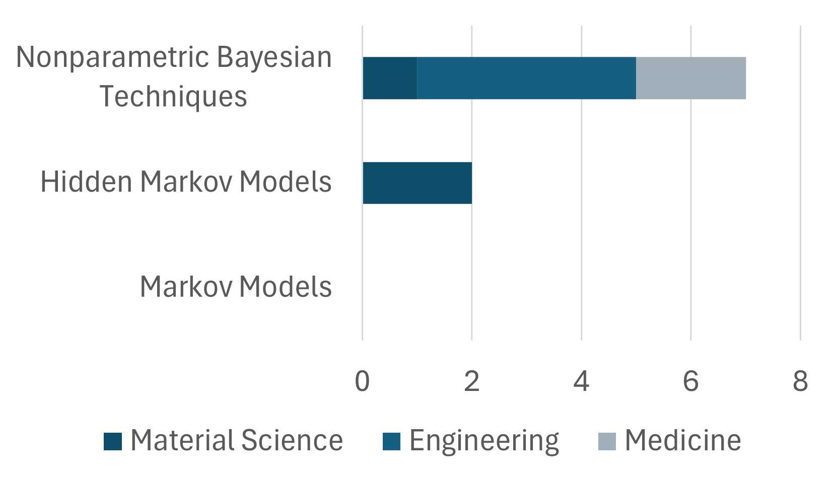
(c) Factor Analysis

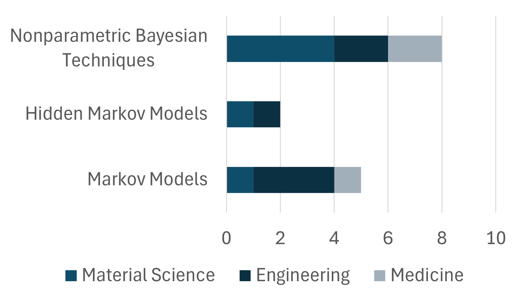
(d) MCMC and probabilistic programming

Figure 5: Combination of statistical inference and dynamic prediction methods

There is no specific relevance mentioned for the combination of Regression Analysis and Markov Models in any of the studied disciplines. The combination of Bayesian statistics and Hidden Markov Models is applicable in all three disciplines, with higher relevance in Engineering and Medicine. This suggests that these techniques can be effectively used together to analyze and model complex systems. The combination of Marcov Chain Monte Carlo and Nonparametric Bayesian Techniques is more applicable in Material Science and Medicine compared to Engineering. This indicates the potential for utilizing these techniques together in solving problems related to sampling from complex probability distributions and analyzing time series data.

5.2.2 Statistical Inference and Machine Learning

Figure 6 presents combinations of techniques from the area of statistical inference methods and machine learning techniques.

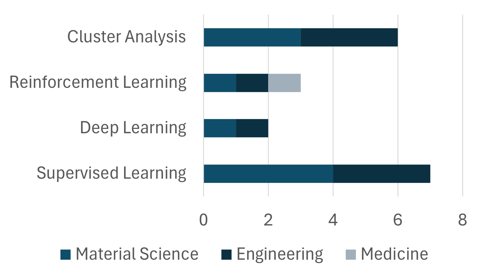
(a) Regression Analysis

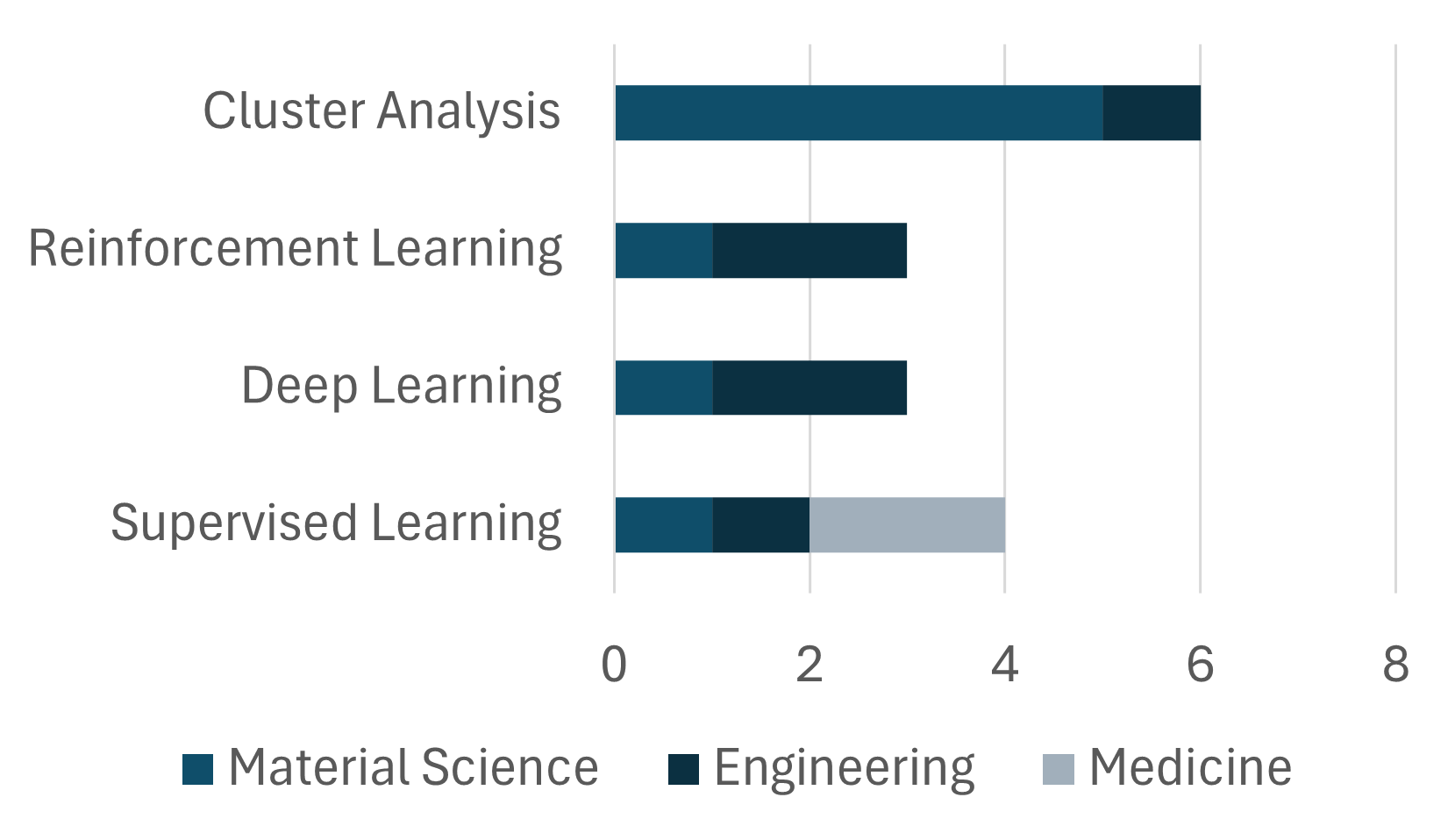
(b) Bayesian statistics

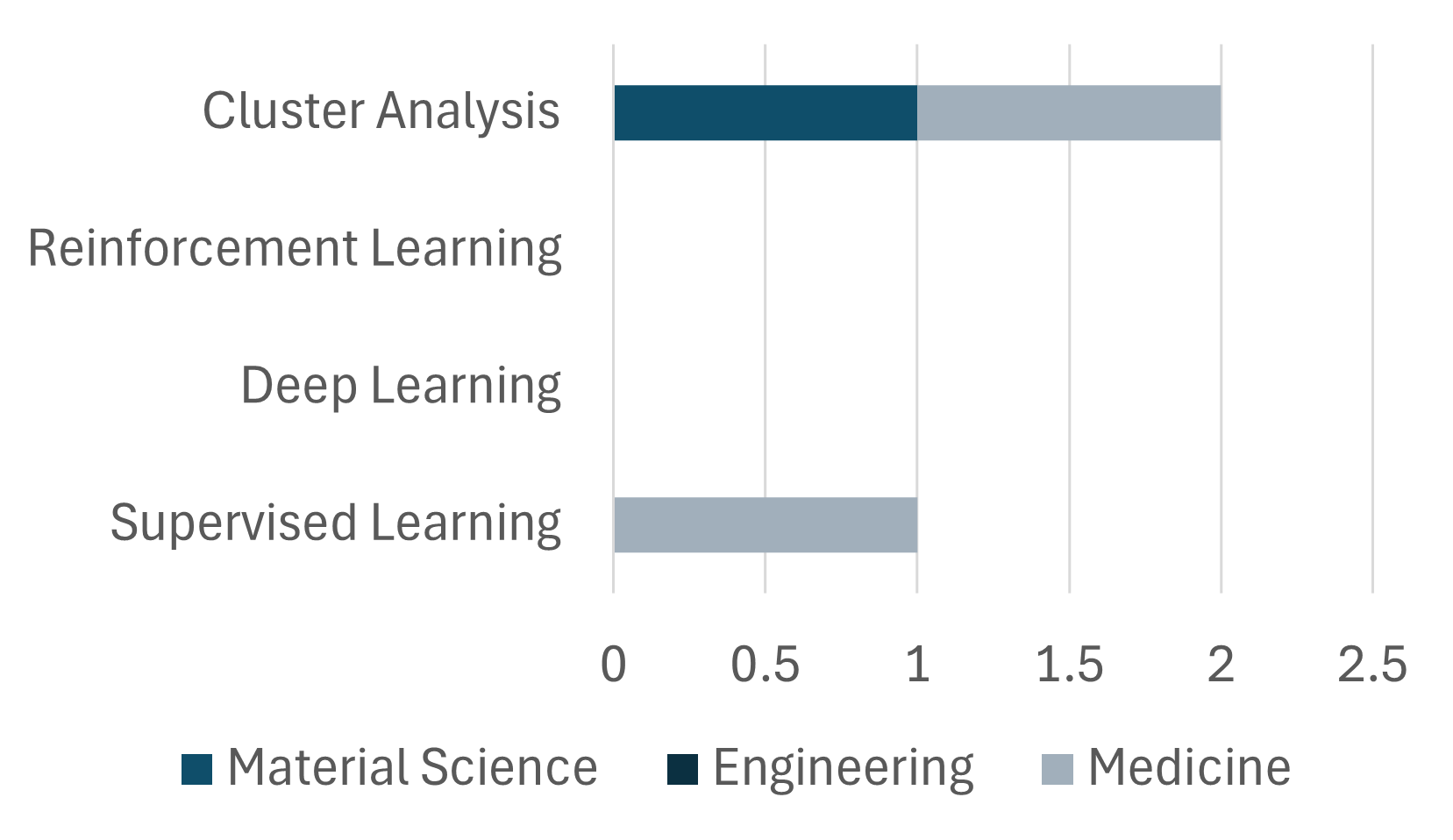
(c) Factor Analysis

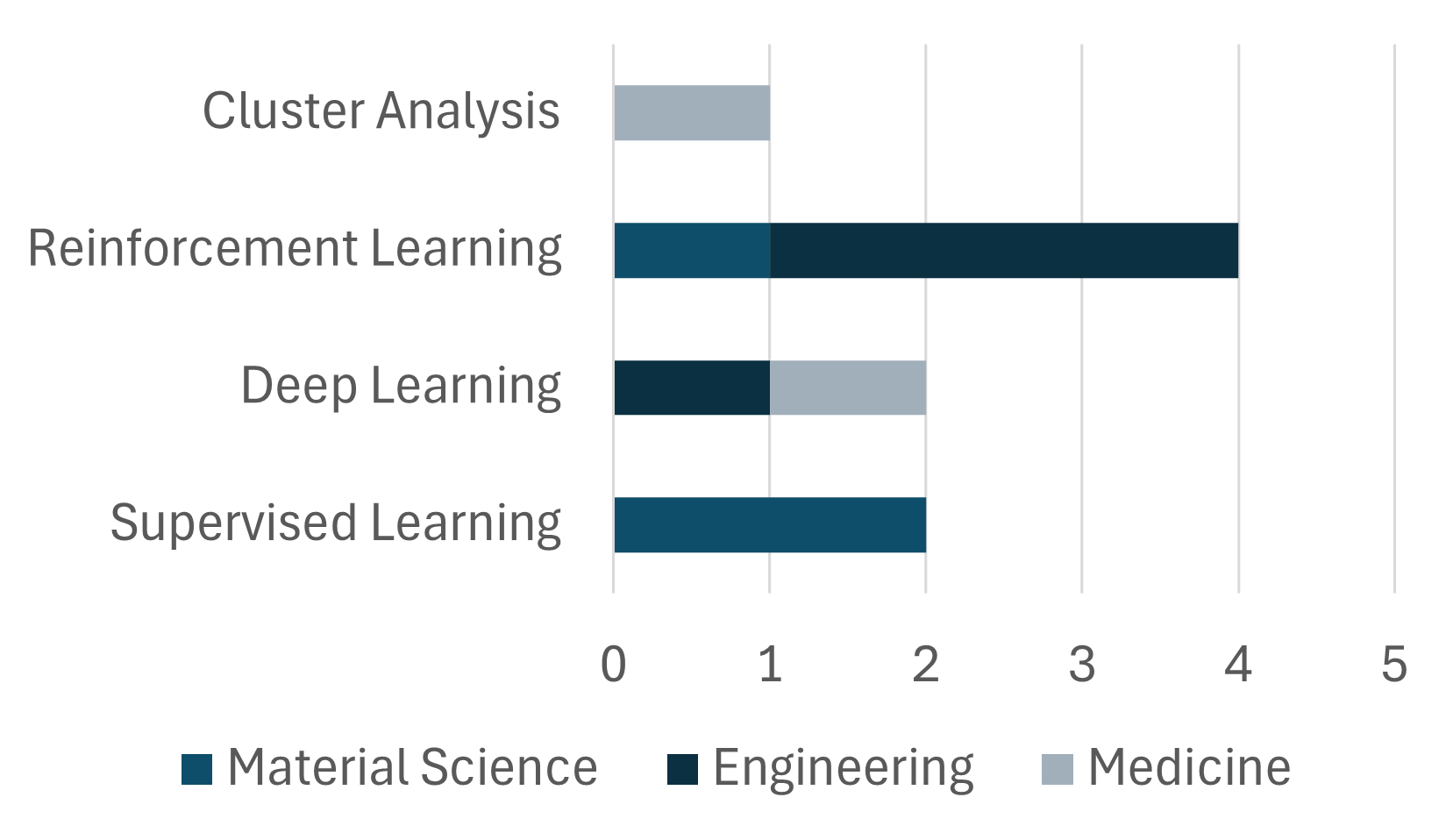
(d) MCMC and probabilistic programming

Figure 6: Combination of statistical inference and machine learning

The combination of Markov Chain Monte Carlo and Probabilistic Programming demonstrates varying relevance across the disciplines. It is more applicable in Engineering for Deep Learning and Reinforcement Learning techniques, while in Material Science, it shows particular relevance for Supervised Learning. Medicine exhibits limited relevance mentioned for Cluster Analysis in this combination. The combination of Bayesian statistics and Supervised Learning is applicable in all three disciplines, with higher relevance in Material Science and Medicine. It finds applications in analyzing and modeling data in the context of supervised learning tasks. The combination of Regression Analysis and Deep Learning is applicable in Material Science and Engineering, with no specific relevance mentioned in Medicine. This suggests the potential integration of regression analysis with deep learning techniques for data analysis.

5.2.3 Dynamic Prediction and Machine Learning

Figure 7 presents the combination of machine learning techniques and dynamic prediction in scientific fields. Figure 7 showcases the relevance of different combinations of methods in various disciplines, including Material Science, Engineering, and Medicine.

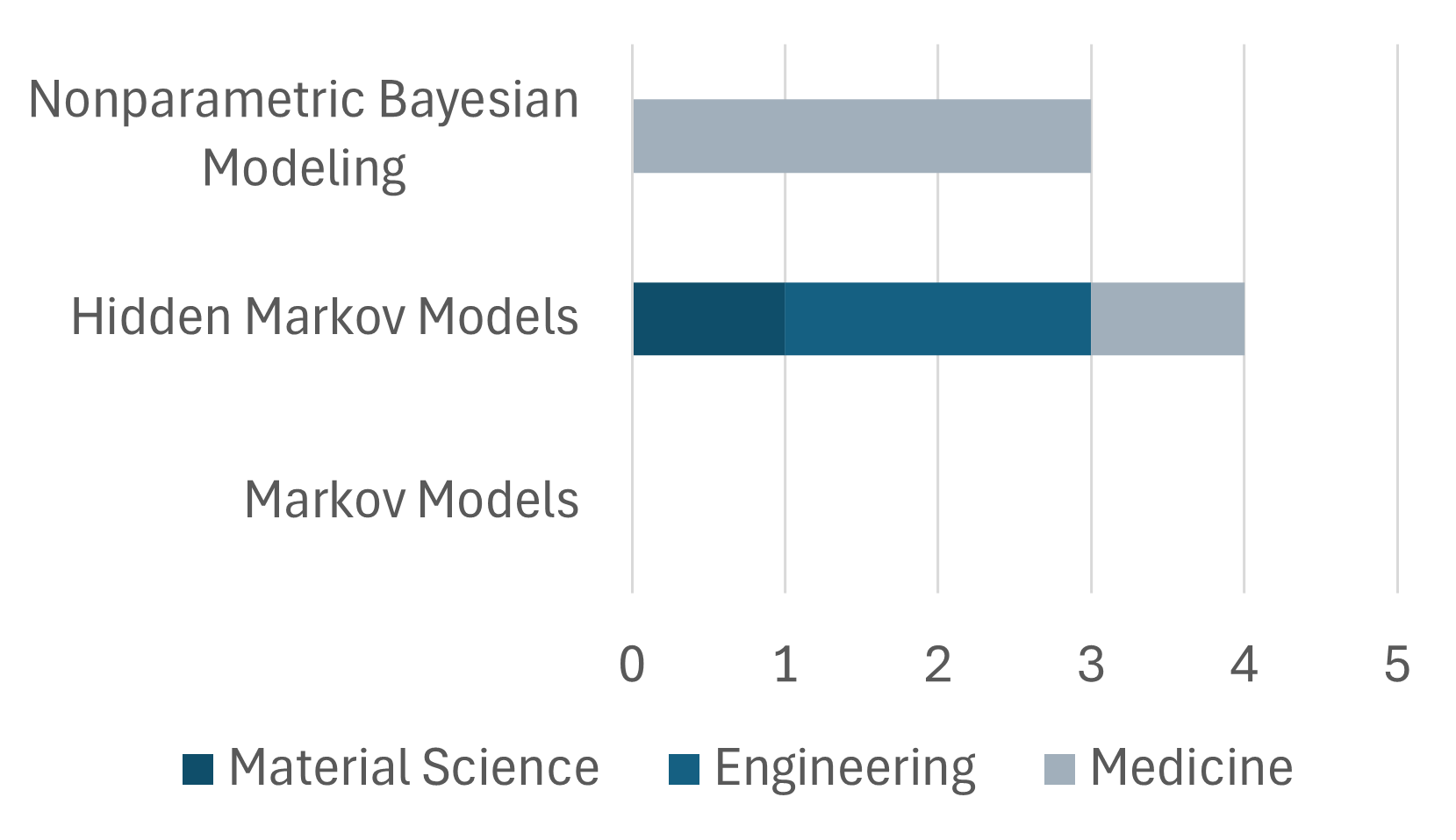
(a) Supervised Learning

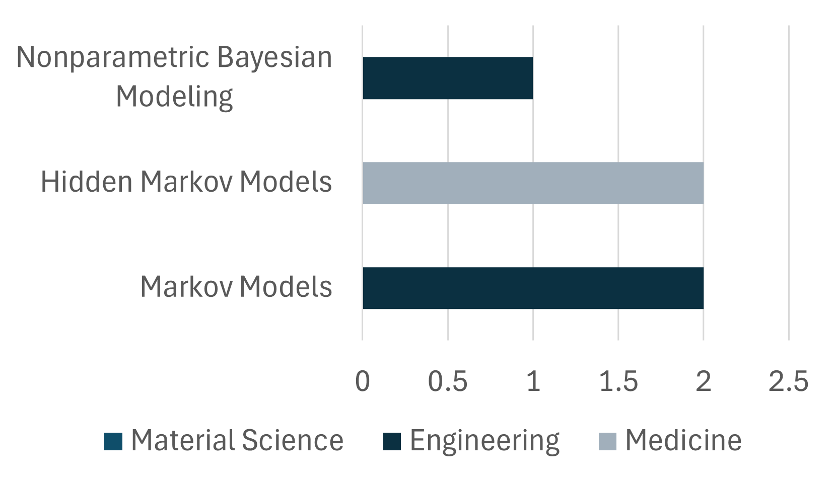
(b) Deep Learning

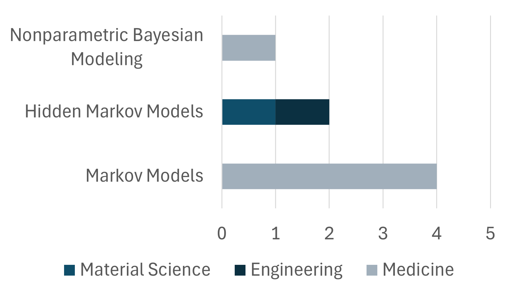
(c) Reinforcement Learning

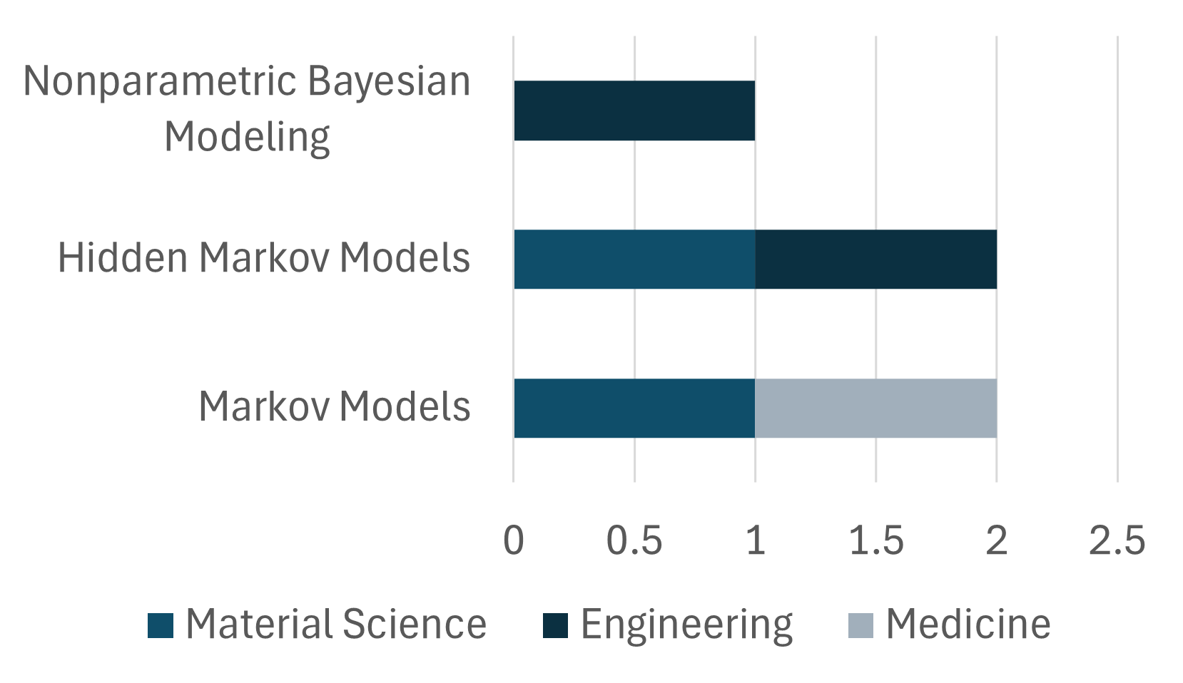
(d) Cluster Analysis

Figure 7: Combination of dynamic prediction and machine learning

The combination of Supervised Learning and Hidden Markov Models is applicable in all three disciplines, with higher relevance in Medicine. This indicates the potential for utilizing these techniques together to analyze and model data in the context of supervised learning tasks. The combination of Deep Learning and Hidden Markov Models is applicable in Engineering and Medicine, with no specific relevance mentioned in Material Science. This suggests the potential integration of deep learning techniques with hidden Markov models for data analysis in these disciplines. The combination of Reinforcement Learning and Markov Models is particularly applicable in Medicine, with higher relevance compared to Material Science and Engineering. This highlights the potential for utilizing reinforcement learning techniques in analyzing and optimizing complex systems within the medical field. The combination of Cluster Analysis and Markov Models is applicable in Material Science, indicating the potential for utilizing cluster analysis techniques in analyzing and identifying patterns in data within this discipline.

6 Discussion and challenges

6.1 Discussion

Table 8 presents an overview of the advantages and disadvantages of the methods for degradation modelling in this paper.

Table 8: Comparison of strengths and weaknesses of each class of methods. Statistical approaches are more interpretable, but can be more costly to compute, however machine learning when provided enough data has great predictive performance.

	Methods	Advantages	Disadvantages
Statistical inference	Regression analysis	Fast computation, Easily interpretable	Linear relationships, Strong assumptions
	Factor analysis	Interpretability	Highest expert knowledge requirements
	MCMC & probabilistic programming	Specification of complicated models,	Mostly Bayesian applications, Computational costs
	Bayesian statistics	Most flexibility, interpretability	Computational problems, untraceablity of direct analytical formulas
Dynamic prediction	Markov models	Widely understood, Good short term predictions	Limited long term accuracy
	Hidden Markov models	Improved prediction quality, more flexibility	Difficult interpretability
	Bayesian time series	Ease of application (esp. Prophet), decomposition of effects	Computational costs
Machine learning	Supervised learning	Flexibility, wide adoption	Difficult interpretability, large dataset requirements
	Deep learning	Flexibility, predictive performance	High dataset requirements, no interpretability, computational costs
	Reinforcement learning	Very promising results	High dataset requirements, no interpretability, computational costs
	Cluster analysis	Limited expert knowledge required, detection of atypical cases	Data requirements, Problems with traceability

6.2 Open challenges

Researchers may explore new modeling techniques which include investigating physics-based models, data-driven models, and hybrid models that combine different approaches to improve the accuracy and reliability of degradation predictions. Additionally, incorporating uncertainty analysis techniques, such as hierarchical nature of degradation processes.

Managing missing data is another critical aspect that needs attention. Strategies such as imputation techniques or robust estimation methods can be employed to handle missing data and ensure accurate model predictions. Furthermore, exploring data fusion and integration techniques, which integrate multiple sources of data such as sensor data, historical records, and expert knowledge, can enhance the understanding and prediction of degradation processes.

Researchers may establish benchmark datasets that are standardized and representative of different degradation scenarios to assess and compare the performance of degradation models. It is essential to define appropriate evaluation metrics that capture the unique characteristics of degradation modeling, considering factors such as prediction accuracy, robustness to uncertainties, and computational efficiency.

Researchers may develop models that capture the dynamic nature of degradation processes to make degradation modeling more applicable in real-world scenarios. These models may consider factors such as aging, maintenance interventions, and changes in operating conditions. Additionally, addressing scalability issues is crucial, as degradation modeling often deals with large-scale systems.

Exploring scalable techniques that can handle numerous components or spatially distributed degradation processes is necessary. Real-time degradation modeling techniques may also be investigated to provide timely predictions and support proactive decision-making in various industries. Through this action researchers can contribute to the continuous improvement and application of degradation modeling, leading to enhanced understanding, prediction, and management of degradation processes in diverse domains.

7 Conclusions

In conclusion, the literature review on degradation modeling methods, including regression analysis, factor analysis, cluster analysis, Markov Chain Monte Carlo with probabilistic programming, Bayesian statistics, hidden Markov models, nonparametric Bayesian modeling of time series, supervised learning, and deep learning, provides valuable insights into the diverse applications and approaches in the field. The review encompasses a comprehensive exploration of degradation modeling across various domains, including material science, power engineering, and medicine.

The review highlights the significance of understanding degradation patterns, optimizing maintenance strategies, and improving overall process efficiency in different domains. It emphasizes the critical role of degradation modeling in analyzing degradation mechanisms, optimizing treatment strategies, and predicting disease progression to improve patient outcomes in the field of Medicine. Additionally, the review underscores the importance of employing statistical inference, dynamic prediction methods, and machine learning techniques in degradation modeling across different disciplines.

Furthermore, the review sheds light on the potential of hybrid modeling techniques, such as the combination of statistical inference and dynamic prediction, statistical inference and machine learning, and dynamic prediction and machine learning, to enhance the understanding and prediction of degradation processes.

The review provides a foundation for understanding the common themes and methods employed in degradation modeling, as evidenced by the overview of various degradation models, their references, methods, and applications. It also offers valuable insights into the preferences and popularity of specific techniques in particular fields, as demonstrated by the number of applications of individual techniques from the Dynamic prediction methods method in each discipline.

Overall, the review serves as a comprehensive resource for researchers and practitioners in the field of degradation modeling, offering a rich understanding of the methods, applications, and implications across diverse domains.

8 Acknowledgments

Work of Anna Jarosz and Jerzy Baranowski partially realised in the scope of project titled ”Process Fault Prediction and Detection”. Project was financed by The National Science Centre on the base of decision no. UMO-2021/41/B/ST7/03851. Part of work was funded by AGH’s Research University Excellence Initiative under project “DUDU - Diagnostyka Uszkodzeń i Degradacji Urzadzeń”.

Marta Zagorowska gratefully acknowledges funding from Marie Curie Horizon Postdoctoral Fellowship project RELIC (grant no 101063948).

References

References

- [1] M. Zagorowska, O. Wu, J. R. Ottewill, M. Reble, N. F. Thornhill, A survey of models of degradation for control applications, Annual Reviews in Control 50 (2020) 150–173.
- [2] D.-H. Xia, S. Song, L. Tao, Z. Qin, Z. Wu, Z. Gao, J. Wang, W. Hu, Y. Behnamian, J.-L. Luo, material degradation assessed by digital image processing: Fundamentals, progresses, and challenges, Journal of Materials Science & Technology 53 (2020) 146–162.
- [3] ISO 10993-13:2010, Biological evaluation of medical devices. Part 13: Identification and quantification of degradation products from polymeric medical devices, Standard, International Organization for Standardization, Geneva, CH (2010).
- [4] ISO 10993-1:2018, Biological evaluation of medical devicesPart 1: Evaluation and testing within a risk management process, Standard, International Organization for Standardization, Geneva, CH (2018).
- [5] ISO 14971:2019, Medical devices — Application of risk management to medical devices, Standard, International Organization for Standardization, Geneva, CH (2019).
- [6] ISO 13485:2016, Medical devices — Quality management systems — Requirements for regulatory purposes, Standard, International Organization for Standardization, Geneva, CH (2016).
- [7] ISO 55000:2014, Asset management — Overview, principles and terminology, Standard, International Organization for Standardization, Geneva, CH (2014).
- [8] ISO 9001:2015, Quality management systems — Requirements, Standard, International Organization for Standardization, Geneva, CH (2015).
- [9] ISO 14001:2015, Environmental management systems — Requirements with guidance for use, Standard, International Organization for Standardization, Geneva, CH (2015).
- [10] ISO 50001:2018, Energy management systems — Requirements with guidance for use, Standard, International Organization for Standardization, Geneva, CH (2018).
- [11] ISO 15156-1:2015, Petroleum and natural gas industries — Materials for use in H2S-containing environments in oil and gas production. Part 1: General principles for selection of cracking-resistant materials, Standard, International Organization for Standardization, Geneva, CH (2015).
- [12] ISO 6892-1:2019, Metallic materials — Tensile testingPart 1: Method of test at room temperature, Standard, International Organization for Standardization, Geneva, CH (2019).
- [13] ISO 11469:2000, Plastics — Generic identification and marking of plastics products, Standard, International Organization for Standardization, Geneva, CH (2000).
- [14] ISO 14040:2006, Environmental management — Life cycle assessment — Principles and framework, Standard, International Organization for Standardization, Geneva, CH (2006).
- [15] M. K. Habib, S. A. Ayankoso, F. Nagata, Data-driven modeling: Concept, techniques, challenges and a case study, in: 2021 IEEE International Conference on Mechatronics and Automation (ICMA), 2021, pp. 1000–1007.
- [16] D. Solomatine, L. See, R. Abrahart, Data-driven modelling: Concepts, approaches and experiences, in: R. J. Abrahart, L. M. See, D. P. Solomatine (Eds.), Practical Hydroinformatics: Computational Intelligence and Technological Developments in Water Applications, Springer Berlin Heidelberg, Berlin, Heidelberg, 2008, Ch. 2, pp. 17–30.
- [17] P. Stoica, Y. Selen, Model-order selection: a review of information criterion rules, IEEE Signal Processing Magazine 21 (4) (2004) 36–47.
- [18] Z. Xu, J. H. Saleh, Machine learning for reliability engineering and safety applications: Review of current status and future opportunities, Reliability Engineering & System Safety 211 (2021) 107530.
- [19] S. Ghosal, A. van der Vaart, Fundamentals of nonparametric Bayesian inference, Cambridge University Press, 2017.
- [20] R. O. Cardenas, Bayesian inference: Observations and applications, Nova Science Publishers, 2018.
- [21] N. Heard, An introduction to Bayesian inference, methods and computation, Springer, 2021.
- [22] K.-R. Koch, Introduction to bayesian statistics, Springer, 2007.
- [23] S.-K. Au, Operational modal analysis: Modeling, Bayesian inference, uncertainty laws, Springer, 2017.
- [24] D. Barber, A. T. Cemgil, S. Chiappa, Bayesian time series models, Vol. 9780521196765, Cambridge University Press, 2011.
- [25] L. Ceniga, Analytical Models of Coherent-Interface-Induced Stresses in Composite Materials III, nova, 2021.
- [26] H. Dong, Z. Ding, S. Zhang, Deep reinforcement learning: Fundamentals, research and applications, Springer, 2020.
- [27] T. Jo, Machine learning foundations: Supervised, unsupervised, and advanced learning, Springer, 2021.
- [28] J. Gao, Nonlinear time series: Semiparametric and nonparametric methods, Chapman & Hall, 2007.
- [29] C. Hua, Reinforcement Learning Aided Performance Optimization of Feedback Control Systems, Springer, 2021.
- [30] M. Baron, Probability and Statistics for Computer Scientists, Third Edition, CRC Press, 2019.
- [31] F. Riguzzi, Foundations of probabilistic logic programming: Languages, semantics, inference and learning - second edition, River Publishers, 2022.
- [32] S. Theodoridis, Machine Learning: A Bayesian and Optimization Perspective, Second Edition, Academic Press, 2020.
- [33] S. Brooks, A. Gelman, G. L. Jones, X.-L. Meng, Handbook of Markov Chain Monte Carlo, Chapman and Hall/CRC, 2011.
- [34] N. Firdaus, H. Ab-Samat, B. T. Prasetyo, Maintenance strategies and energy efficiency: a review, Journal of Quality in Maintenance Engineering 29 (3) (2023) 640 – 665.
- [35] E. Jaime-Barquero, E. Bekaert, J. Olarte, E. Zulueta, J. M. Lopez-Guede, Artificial intelligence opportunities to diagnose degradation modes for safety operation in lithium batteries, Batteries 9 (7) (2023).
- [36] O. A. Alimi, E. L. Meyer, O. I. Olayiwola, Solar photovoltaic modules’ performance reliability and degradation analysis—a review, Energies 15 (16) (2022).
- [37] T. Berghout, M. Benbouzid, A systematic guide for predicting remaining useful life with machine learning, Electronics (Switzerland) 11 (7) (2022).
- [38] S. Zhao, M. Tayyebi, M. Yarigarravesh, G. Hu, A review of magnesium corrosion in bio-applications: mechanism, classification, modeling, in-vitro, and in-vivo experimental testing, and tailoring mg corrosion rate, Journal of Materials Science 58 (30) (2023) 12158 – 12181.
- [39] K. Xue, J. Yang, M. Yang, D. Wang, An improved generic hybrid prognostic method for RUL prediction based on PF-LSTM learning, IEEE Transactions on Instrumentation and Measurement 72 (2023).
- [40] L. Papargyri, M. Theristis, B. Kubicek, T. Krametz, C. Mayr, P. Papanastasiou, G. E. Georghiou, Modelling and experimental investigations of microcracks in crystalline silicon photovoltaics: A review, Renewable Energy 145 (2020) 2387 – 2408.
- [41] M. Mondal, G. Kumbhar, Detection, measurement, and classification of partial discharge in a power transformer: Methods, trends, and future research, IETE Technical Review (Institution of Electronics and Telecommunication Engineers, India) 35 (5) (2018) 483 – 493.
- [42] M. Zhang, S. Yang, Contemporary machine learning approaches towards biomechanical analysis in the diagnosis and prognosis prediction of knee osteoarthritis: A systematic review, Undergraduate Research in Natural and Clinical Science and Technology Journal 8 (1) (2024).
- [43] P. S. Chakurkar, D. Vora, S. Patil, S. Mishra, K. Kotecha, Data-driven approach for ai-based crack detection: techniques, challenges, and future scope, Frontiers in Sustainable Cities 5 (2023).
- [44] Y. Li, S. Wang, M. M. Tomovic, C. Zhang, Erosion degradation characteristics of a linear electro-hydrostatic actuator under a high-frequency turbulent flow field, Chinese Journal of Aeronautics 31 (5) (2018) 914 – 926.
- [45] B. K. Kurz R., Degradation in gas turbine systems, Journal of Engineering for Gas Turbines and Power 123 (1) (2001) 70 – 77.
- [46] D. C. Montgomery, E. A. Peck, G. G. Vining, Introduction to Linear Regression Analysis, 5th Edition, Wiley, Hoboken, NJ, 2012.
- [47] Y. Yu, X. Si, C. Hu, J. Zheng, J. Zhang, Online remaining-useful-life estimation with a Bayesian-updated expectation-conditional-maximization algorithm and a modified Bayesian-model-averaging method, Science China Information Sciences 64 (1) (2021).
- [48] I. Bejaoui, D. Bruneo, M. G. Xibilia, A data-driven prognostics technique and RUL prediction of rotating machines using an exponential degradation model, 7th International Conference on Control, Decision and Information Technologies, CoDIT 2020 (2020) 703 – 708.
- [49] D. J. Bartholomew, M. Knott, I. Moustaki, Latent Variable Models and Factor Analysis: A Unified Approach, 2nd Edition, Wiley, Chichester, UK, 2011.
- [50] Z. Xu, Y. Hong, R. Jin, Nonlinear general path models for degradation data with dynamic covariates, Applied Stochastic Models in Business and Industry 32 (2) (2016) 153 – 167.
- [51] L. Lu, B. Wang, Y. Hong, Z. Ye, General path models for degradation data with multiple characteristics and covariates, Technometrics 63 (3) (2021) 354 – 369.
- [52] A. Gelman, J. B. Carlin, H. S. Stern, D. B. Dunson, A. Vehtari, D. B. Rubin, Bayesian Data Analysis, 3rd Edition, CRC Press, Boca Raton, FL, 2013.
- [53] A. H. Dadash, N. Björsell, Optimal degradation-aware control using process-controlled sparse Bayesian learning, Processes 11 (11) (2023).
- [54] A. F. Shahraki, O. P. Yadav, H. Liao, A review on degradation modelling and its engineering applications, International Journal of Performability Engineering 13 (3) (2017) 299 – 314.
- [55] R. M. Neal, Mcmc using hamiltonian dynamics, in: S. Brooks, A. Gelman, G. L. Jones, X.-L. Meng (Eds.), Handbook of Markov Chain Monte Carlo, Chapman & Hall/CRC, London, 2011, pp. 113–162.
- [56] F. Tamssaouet, K. T. Nguyen, K. Medjaher, M. E. Orchard, System-level failure prognostics: Literature review and main challenges, Proceedings of the Institution of Mechanical Engineers, Part O: Journal of Risk and Reliability 237 (3) (2023) 524 – 545.
- [57] J. R. Norris, Markov Chains, Cambridge University Press, Cambridge, UK, 1997.
- [58] H. Zhou, K. Lange, Composition Markov chains of multinomial type, Advances in Applied Probability 41 (1) (2009) 270 – 291.
- [59] Z. Bulinski, H. R. Orlande, Estimation of the non-linear diffusion coefficient with Markov Chain Monte Carlo method based on the integral information, International Journal of Numerical Methods for Heat and Fluid Flow 27 (3) (2017) 639 – 659.
- [60] Z. Zhang, S. Xu, Y. Guo, Y. Chu, Robust adaptive output-feedback control for a class of nonlinear systems with time-varying actuator faults, International Journal of Adaptive Control and Signal Processing 24 (9) (2010) 743 – 759.
- [61] L. R. Rabiner, A tutorial on hidden markov models and selected applications in speech recognition, Proceedings of the IEEE 77 (2) (1989) 257–286.
- [62] D.-B. Du, J.-X. Zhang, Z.-J. Zhou, X.-S. Si, C.-H. Hu, Estimating remaining useful life for degrading systems with large fluctuations, Journal of Control Science and Engineering 2018 (2018).
- [63] S. Baldi, T. L. Quang, O. Holub, P. Endel, Real-time monitoring energy efficiency and performance degradation of condensing boilers, Energy Conversion and Management 136 (2017) 329 – 339.
- [64] S. J. Taylor, B. Letham, Forecasting at scale, The American Statistician 72 (1) (2018) 37–45.
- [65] Y. Ding, Q. Yang, C. B. King, Y. Hong, A general accelerated destructive degradation testing model for reliability analysis, IEEE Transactions on Reliability 68 (4) (2019) 1272 – 1282.
- [66] C. Zhang, Y. Ma, Ensemble machine learning: Methods and applications, Springer, 2012.
- [67] T. Hastie, R. Tibshirani, J. Friedman, The Elements of Statistical Learning: Data Mining, Inference, and Prediction, 2nd Edition, Springer, New York, NY, 2009.
- [68] A. Qin, Q. Zhang, Q. Hu, G. Sun, J. He, S. Lin, Remaining useful life prediction for rotating machinery based on optimal degradation indicator, Shock and Vibration 2017 (2017).
- [69] R. Kang, W. Gong, Y. Chen, Model-driven degradation modeling approaches: Investigation and review, Chinese Journal of Aeronautics 33 (4) (2020) 1137 – 1153.
- [70] I. Goodfellow, Y. Bengio, A. Courville, Deep Learning, MIT Press, Cambridge, MA, 2016.
- [71] R. S. Sutton, A. G. Barto, Reinforcement Learning: An Introduction, 2nd Edition, MIT Press, Cambridge, MA, 2018.
- [72] L. Samaranayake, S. Longo, Degradation control for electric vehicle machines using nonlinear model predictive control, IEEE Transactions on Control Systems Technology 26 (1) (2018) 89 – 101.
- [73] G. Fang, R. Pan, Y. Hong, Copula-based reliability analysis of degrading systems with dependent failures, Reliability Engineering and System Safety 193 (2020).
- [74] L. Kaufman, P. J. Rousseeuw, Finding Groups in Data: An Introduction to Cluster Analysis, 1st Edition, Wiley, Hoboken, NJ, 2005.
- [75] M. J. de Lima, C. D. Paredes Crovato, R. I. Goytia Mejia, R. da Rosa Righi, G. de Oliveira Ramos, C. André da Costa, G. Pesenti, HealthMon: An approach for monitoring machines degradation using time-series decomposition, clustering, and metaheuristics, Computers and Industrial Engineering 162 (2021).
- [76] A. Jayakumar, D. K. Madheswaran, N. M. Kumar, A critical assessment on functional attributes and degradation mechanism of membrane electrode assembly components in direct methanol fuel cells, Sustainability (Switzerland) 13 (24) (2021).
- [77] X. Wu, C. Sen, H. Wang, X. Wang, Y. Wu, M. U. Khan, L. Mao, F. Jiang, T. Xu, G. Zhang, B. Hoex, Addressing sodium ion-related degradation in SHJ cells by the application of nano-scale barrier layers, Solar Energy Materials and Solar Cells 264 (2024).
- [78] G. Rodríguez-Bravo, M. Vite-Torres, J. Godínez-Salcedo, Corrosion rate and wear mechanisms comparison for AISI 410 stainless steel exposed to pure corrosion and abrasion-corrosion in a simulated marine environment, Tribology in Industry 41 (3) (2019) 394 – 400.
- [79] J. Liu, X. Luo, Q. Chen, Degradation of steel rebar tensile properties affected by longitudinal non-uniform corrosion, Materials 16 (7) (2023).
- [80] V. A. Hosseini, L. Karlsson, S. Wessman, N. Fuertes, Effect of sigma phase morphology on the degradation of properties in a super duplex stainless steel, Materials 11 (6) (2018).
- [81] B. Zeller-Plumhoff, D. Laipple, H. Slominska, K. Iskhakova, E. Longo, A. Hermann, S. Flenner, I. Greving, M. Storm, R. Willumeit-Römer, Evaluating the morphology of the degradation layer of pure magnesium via 3D imaging at resolutions below 40 nm, Bioactive Materials 6 (12) (2021) 4368 – 4376.
- [82] H. Al Mahdi, P. G. Leahy, A. P. Morrison, Experimentally derived models to detect onset of shunt resistance degradation in photovoltaic modules, Energy Reports 10 (2023) 604 – 612.
- [83] F. Yang, M. M. Yuan, W. J. Qiao, N. N. Li, B. Du, Mechanical degradation of Q345 weathering steel and Q345 carbon steel under acid corrosion, Advances in Materials Science and Engineering 2022 (2022).
- [84] R. P. Alessio, N. M. Andre, S. M. Goushegir, J. F. dos Santos, J. A. E. Mazzaferro, S. T. Amancio-Filho, Prediction of the mechanical and failure behavior of metal-composite hybrid joints using cohesive surfaces, Materials Today Communications 24 (2020).
- [85] S. Elahi, F. M. Sofiani, S. Chaudhuri, J. Balbin, N. Larrosa, W. De Waele, Investigation of the effect of pitting corrosion on the fatigue strength degradation of structural steel using a short crack model, Procedia Structural Integrity 51 (2023) 30 – 36.
- [86] X. Li, S. Li, D. Wei, L. Si, K. Yu, K. Yan, Dynamics simulation-driven fault diagnosis of rolling bearings using security transfer support matrix machine, Reliability Engineering and System Safety 243 (2024).
- [87] T. Jain, K. Verma, Reliability based computational model for stochastic unit commitment of a bulk power system integrated with volatile wind power, Reliability Engineering and System Safety 244 (2024).
- [88] T. Han, Y.-F. Li, Out-of-distribution detection-assisted trustworthy machinery fault diagnosis approach with uncertainty-aware deep ensembles, Reliability Engineering and System Safety 226 (2022).
- [89] J. A. Osara, M. D. Bryant, A thermodynamic model for lithium-ion battery degradation: Application of the degradation-entropy generation theorem, Inventions 4 (2) (2019).
- [90] P. Fang, A. Zhang, X. Sui, D. Wang, L. Yin, Z. Wen, Analysis of performance degradation in lithium-ion batteries based on a lumped particle diffusion model, ACS Omega 8 (36) (2023) 32884 – 32891.
- [91] N. I. Shchurov, S. I. Dedov, B. V. Malozyomov, A. A. Shtang, N. V. Martyushev, R. V. Klyuev, S. N. Andriashin, Degradation of lithium-ion batteries in an electric transport complex, Energies 14 (23) (2021).
- [92] D.-I. Stroe, M. Swierczynski, S. K. Kær, R. Teodorescu, Degradation behavior of lithium-ion batteries during calendar ageing - the case of the internal resistance increase, IEEE Transactions on Industry Applications 54 (1) (2018) 517 – 525.
- [93] C. Oria, C. Méndez, I. Carrascal, D. Ferreño, A. Ortiz, Degradation of the compression strength of spacers made of high-density pressboard used in power transformers under the influence of thermal ageing, Cellulose 30 (10) (2023) 6539 – 6558.
- [94] D. Karunathilake, M. Vilathgamuwa, Y. Mishra, P. Corry, T. Farrell, S. S. Choi, Degradation-conscious multiobjective optimal control of reconfigurable li-ion battery energy storage systems, Batteries 9 (4) (2023).
- [95] J. Xu, R. D. Deshpande, J. Pan, Y.-T. Cheng, V. S. Battaglia, Electrode side reactions, capacity loss and mechanical degradation in lithium-ion batteries, Journal of the Electrochemical Society 162 (10) (2015) A2026 – A2035.
- [96] D. Liu, Y. Luo, Y. Peng, X. Peng, M. Pecht, Lithium-ion battery remaining useful life estimation based on nonlinear AR model combined with degradation feature, in: Proceedings of the Annual Conference of the Prognostics and Health Management Society 2012, PHM 2012, 2012, pp. 336 – 342.
- [97] L. Spitthoff, M. S. Wahl, J. J. Lamb, P. R. Shearing, P. J. S. Vie, O. S. Burheim, On the relations between lithium-ion battery reaction entropy, surface temperatures and degradation, Batteries 9 (5) (2023).
- [98] K. Su, B. Deng, S. Tang, X. Sun, P. Fang, X. Si, X. Han, Remaining useful life prediction of lithium-ion batteries based on a cubic polynomial degradation model and envelope extraction, Batteries 9 (9) (2023).
- [99] S. B. Narale, A. Verma, S. Anand, Structure and degradation of aluminum electrolytic capacitors, in: 2019 National Power Electronics Conference, NPEC 2019, 2019, pp. 1–6.
- [100] S. Kohtz, J. Zhao, A. Renteria, A. Lalwani, Y. Xu, X. Zhang, K. S. Haran, D. Senesky, P. Wang, Optimal sensor placement for permanent magnet synchronous motor condition monitoring using a digital twin-assisted fault diagnosis approach, Reliability Engineering and System Safety 242 (2024).
- [101] A. E. Chaleshtori, A. Aghaie, A novel bearing fault diagnosis approach using the Gaussian mixture model and the weighted principal component analysis, Reliability Engineering and System Safety 242 (2024).
- [102] D. Dumanlidağ, D. Keleş, G. Oktay, C. Koşay, Effects of vertebral fusion on levels of pro-inflammatory and catabolic mediators in a rabbit model of intervertebral disc degeneration, Acta Orthopaedica et Traumatologica Turcica 55 (3) (2021) 246 – 252.
- [103] L. Vernizzi, C. Paiardi, G. Licata, T. Vitali, S. Santarelli, M. Raneli, V. Manelli, M. Rizzetto, M. Gioria, M. E. Pasini, D. Grifoni, M. A. Vanoni, C. Gellera, F. Taroni, P. Bellosta, Glutamine synthetase 1 increases autophagy lysosomal degradation of mutant huntingtin aggregates in neurons, ameliorating motility in a drosophila model for Huntington’s disease, Cells 9 (1) (2020).
- [104] Z. Wang, X. Li, P. Yu, Y. Zhu, F. Dai, Z. Ma, X. Shen, H. Jiang, J. Liu, Role of autophagy and pyroptosis in intervertebral disc degeneration, Journal of Inflammation Research 17 (2024) 91 – 100.
- [105] K. Wang, D. Yao, Y. Li, M. Li, W. Zeng, Z. Liao, E. Chen, S. Lu, K. Su, Z. Che, Y. Liang, P. Wang, L. Huang, TAK-715 alleviated IL-1-induced apoptosis and ECM degradation in nucleus pulposus cells and attenuated intervertebral disc degeneration ex vivo and in vivo, Arthritis Research and Therapy 25 (1) (2023).
- [106] P. T. Nguyen, L. Manuel, Uncertainty quantification in low-probability response estimation using sliced inverse regression and polynomial chaos expansion, Reliability Engineering and System Safety 242 (2024).
- [107] W. Lin, Y. Wang, S. Lampkin, S. G. Prasad, O. Zhupanska, B. Davidson, Bond strength degradation of adhesive-bonded CFRP composite lap joints after lightning strike, in: 36th Technical Conference of the American Society for Composites 2021: Composites Ingenuity Taking on Challenges in Environment-Energy-Economy, ASC 2021, Vol. 1, 2021, pp. 37 – 49.
- [108] R. Amaya-Gómez, J. Riascos-Ochoa, F. Muñoz, E. Bastidas-Arteaga, F. Schoefs, M. Sánchez-Silva, Modeling of pipeline corrosion degradation mechanism with a Lévy process based on ILI (in-line) inspections, International Journal of Pressure Vessels and Piping 172 (2019) 261 – 271.
- [109] W. Weng, X. Xie, Y. Lei, Probability-based performance degradation model and constitutive model for the buckling behavior of corroded steel bars, Sustainability (Switzerland) 15 (9) (2023).
- [110] C. Liu, J. Chen, High temperature degradation mechanism of concrete with plastering layer, Materials 15 (2) (2022).
- [111] J. Nepal, H.-P. Chen, A. M. Alani, Analytical modelling of bond strength degradation due to reinforcement corrosion, Key Engineering Materials 569-570 (2013) 1060 – 1067.
- [112] P. Schneider, M. Batool, A. O. Godoy, R. Singh, D. Gerteisen, J. Jankovic, N. Zamel, Impact of platinum loading and layer thickness on cathode catalyst degradation in PEM fuel cells, Journal of the Electrochemical Society 170 (2) (2023).
- [113] C. S. Kulkarni, G. Biswas, X. Koutsoukos, A prognosis case study for electrolytic capacitor degradation in DC–DC converters, in: Annual Conference of the Prognostics and Health Management Society, PHM 2009, 2009.
- [114] J. Chen, C. Lin, B. Yao, L. Yang, H. Ge, Intelligent fault diagnosis of rolling bearings with low-quality data: A feature significance and diversity learning method, Reliability Engineering and System Safety 237 (2023).
- [115] Y. Qu, H. Zhao, S. Zhao, L. Ma, Z. Mi, Power transformer oil–paper insulation degradation modelling and prediction method based on functional principal component analysis, IET Science, Measurement and Technology 16 (8) (2022) 441 – 453.
- [116] J. M. Reniers, G. Mulder, D. A. Howey, Review and performance comparison of mechanical-chemical degradation models for lithium-ion batteries, Journal of the Electrochemical Society 166 (14) (2019) A3189 – A3200.
- [117] M. Nicolai, M. Zanuccoli, M. Galiazzo, M. Bertazzo, E. Sangiorgi, C. Fiegna, Simulation study of light-induced, current-induced degradation and recovery on PERC solar cells, Energy Procedia 92 (2016) 153 – 159.
- [118] M. Godinho, V. Carvalho, M. Matos, P. Fernandes, A. Castro, Computational modeling of lumbar disc degeneration before and after spinal fusion, Clinical Biomechanics 90 (2021).
- [119] T. Liang, B. Gao, J. Zhou, X. Qiu, J. Qiu, T. Chen, Y. Liang, W. Gao, X. Qiu, Y. Lin, Constructing intervertebral disc degeneration animal model: A review of current models, Frontiers in Surgery 9 (2022).
- [120] A. Ewald, A. Fuchs, L. Boegelein, J.-P. Grunz, K. Kneist, U. Gbureck, S. Hoelscher-Doht, Degradation and bone-contact biocompatibility of two drillable magnesium phosphate bone cements in an in vivo rabbit bone defect model, Materials 16 (13) (2023).
- [121] X. Sheng, Q. Guo, J. Yu, Y. Xu, Experimental research on the effect of microRNA-21 inhibitor on a rat model of intervertebral disc degeneration, Experimental and Therapeutic Medicine 16 (1) (2018) 67 – 72.
- [122] Z. Geng, J. Wang, G. Chen, J. Liu, J. Lan, Z. Zhang, J. Miao, Gut microbiota and intervertebral disc degeneration: a bidirectional two-sample Mendelian randomization study, Journal of Orthopaedic Surgery and Research 18 (1) (2023).
- [123] K. Rashid, I. K. Sundar, J. Gerloff, D. Li, I. Rahman, Lung cellular senescence is independent of aging in a mouse model of COPD/emphysema, Scientific Reports 8 (1) (2018).
- [124] P. Song, S. Li, H. Wu, R. Gao, G. Rao, D. Wang, Z. Chen, B. Ma, H. Wang, N. Sui, H. Deng, Z. Zhang, T. Tang, Z. Tan, Z. Han, T. Lu, Y. Zhu, Q. Chen, Parkin promotes proteasomal degradation of p62: implication of selective vulnerability of neuronal cells in the pathogenesis of Parkinson’s disease, Protein and Cell 7 (2) (2016) 114 – 129.
- [125] Z. Yang, P. Baraldi, E. Zio, A method for fault detection in multi-component systems based on sparse autoencoder-based deep neural networks, Reliability Engineering and System Safety 220 (2022).
- [126] D. D’Urso, F. Chiacchio, S. Cavalieri, S. Gambadoro, S. M. Khodayee, Predictive maintenance of standalone steel industrial components powered by a dynamic reliability digital twin model with artificial intelligence, Reliability Engineering and System Safety 243 (2024).
- [127] M. Zheng, Z. Su, D. Wang, E. Pan, Joint maintenance and spare part ordering from multiple suppliers for multicomponent systems using a deep reinforcement learning algorithm, Reliability Engineering and System Safety 241 (2024).
- [128] Y. Hu, L. Zhang, Y. Jiang, K. Peng, Z. Jin, A hybrid method for performance degradation probability prediction of proton exchange membrane fuel cell, Membranes 13 (4) (2023).
- [129] J. Szabelski, R. Karpiński, J. Jonak, M. Frigione, Adhesive joint degradation due to hardener-to-epoxy ratio inaccuracy under varying curing and thermal operating conditions, Materials 15 (21) (2022).
- [130] S. Kaewmala, N. Kamma, S. Buakeaw, W. Limphirat, J. Nash, S. Srilomsak, P. Limthongkul, N. Meethong, Impacts of mg doping on the structural properties and degradation mechanisms of a Li and Mn rich layered oxide cathode for lithium-ion batteries, Scientific Reports 13 (1) (2023).
- [131] T. Meng, Y. Chen, K. Ying, X. Jin, S. Zhan, Deterioration mechanism of concrete under long-term elevated temperature in a metallurgic environment: A case study of the Baosteel company, Case Studies in Construction Materials 14 (2021).
- [132] R. Ueda, K. Sawata, R. Takanashi, Y. Sasaki, T. Sasaki, Degradation of shear performance of screwed joints caused by wood decay, Journal of Wood Science 66 (1) (2020).
- [133] M. C. Silva, F. M. Ferguson, Q. Cai, K. A. Donovan, G. Nandi, D. Patnaik, T. Zhang, H.-T. Huang, D. E. Lucente, B. C. Dickerson, T. J. Mitchison, E. S. Fischer, N. S. Gray, S. J. Haggarty, Targeted degradation of aberrant tau in frontotemporal dementia patient-derived neuronal cell models, eLife 8 (2019).
- [134] S. Chunsheng, Z. Jiaxiang, Y. Mo, S. Erwei, Z. Jinguang, Reconstruction of fiber Bragg grating strain profile used to monitor the stiffness degradation of the adhesive layer in carbon fiber-reinforced plastic single-lap joint, Advances in Mechanical Engineering 9 (3) (2017).
- [135] H. J. Park, N. H. Kim, J.-H. Choi, A robust health prediction using bayesian approach guided by physical constraints, Reliability Engineering and System Safety 244 (2024).
- [136] B. Mitra, A. Singhal, S. Kundu, J. P. Ogle, Analyzing distribution transformer degradation with increased power electronic loads, in: 2023 IEEE Power and Energy Society Innovative Smart Grid Technologies Conference, ISGT 2023, 2023, pp. 1–5.
- [137] W. Li, J. Chen, K. Quade, D. Luder, J. Gong, D. U. Sauer, Battery degradation diagnosis with field data, impedance-based modeling and artificial intelligence, Energy Storage Materials 53 (2022) 391 – 403.
- [138] A. Singh, A. Anurag, S. Anand, Evaluation of vce at inflection point for monitoring bond wire degradation in discrete packaged IGBTs, IEEE Transactions on Power Electronics 32 (4) (2017) 2481 – 2484.
- [139] A. Schiffmacher, D. Strahringer, S. Malasani, J. Wilde, C. Kempiak, A. Lindemann, In situ degradation monitoring methods during lifetime testing of power electronic modules, in: Proceedings - Electronic Components and Technology Conference, Vol. 2021-June, 2021, pp. 895 – 903.
- [140] N. Costa, L. Sánchez, D. Anseán, M. Dubarry, Li-ion battery degradation modes diagnosis via convolutional neural networks, Journal of Energy Storage 55 (2022).
- [141] C. Yu, L. Jiang, J. Yuan, Study of performance degradations in DC–DC converter due to hot carrier stress by simulation, Microelectronics Reliability 46 (9-11) (2006) 1840 – 1843.
- [142] K. Zhao, J. Hu, H. Shao, J. Hu, Federated multi-source domain adversarial adaptation framework for machinery fault diagnosis with data privacy, Reliability Engineering and System Safety 236 (2023).
- [143] M. Streb, M. Ohrelius, A. Siddiqui, M. Klett, G. Lindbergh, Diagnosis and prognosis of battery degradation through re-evaluation and Gaussian process regression of electrochemical model parameters, Journal of Power Sources 588 (2023).
- [144] S. Yamaguchi, A. Masuda, K. Marumoto, K. Ohdaira, Mechanistic understanding of polarization-type potential-induced degradation in crystalline-silicon photovoltaic cell modules, Advanced Energy and Sustainability Research 4 (4) (2023).
- [145] J. W. Snuggs, R. E. Day, F. C. Bach, M. T. Conner, R. A. D. Bunning, M. A. Tryfonidou, C. L. Le Maitre, Aquaporin expression in the human and canine intervertebral disc during maturation and degeneration, JOR Spine 2 (1) (2019).
- [146] P. Rivero-Ríos, J. Madero-Pérez, B. Fernández, S. Hilfiker, Targeting the autophagy/lysosomal degradation pathway in Parkinson’s disease, Current Neuropharmacology 14 (3) (2016) 238 – 249.
- [147] P. Ayala, R. Vivar, R. Montalva, P. Olmos, M. Meneses, G. R. Borzone, Elastin degradation products in acute lung injury induced by gastric contents aspiration, Respiratory Research 19 (1) (2018).
- [148] D. Betancourt, P. Baldion, J. Castellanos, Resin-dentin bonding interface: Mechanisms of degradation and strategies for stabilization of the hybrid layer, International Journal of Biomaterials 2019 (2019).
- [149] C. Shuai, W. Yang, P. Feng, S. Peng, H. Pan, Accelerated degradation of HAP/PLLA bone scaffold by pga blending facilitates bioactivity and osteoconductivity, Bioactive Materials 6 (2) (2021) 490 – 502.
- [150] H. Badet, F. Poineau, Corrosion studies of stainless steel 304 L in nitric acid in the presence of uranyl nitrate: effect of temperature and nitric acid concentration, SN Applied Sciences 2 (3) (2020).
- [151] P. Gupta, M. Streb, A. Siddiqui, M. Klett, G. Lindbergh, P. Gudmundson, Layer-resolved mechanical degradation of a Ni-rich positive electrode, Batteries 9 (12) (2023).
- [152] A. S. Chaudhary, B. Kiran, K. Sivagami, D. Govindarajan, S. Chakraborty, Thermal degradation model of used surgical masks based on machine learning methodology, Journal of the Taiwan Institute of Chemical Engineers 144 (2023).
- [153] A. Dalmau, C. Richard, A. Igual – Muñoz, Degradation mechanisms in martensitic stainless steels: Wear, corrosion and tribocorrosion appraisal, Tribology International 121 (2018) 167 – 179.
- [154] Y. Xiang, M. Deng, F.-Z. Xuan, C.-J. Liu, Experimental study of thermal degradation in ferritic CrNi alloy steel plates using nonlinear Lamb waves, NDT and E International 44 (8) (2011) 768 – 774.
- [155] M. Kudo, J. Takahashi, T. Yamamoto, M. Uchida, Y. Tomita, Multi-scale modeling of degradation behavior for crystalline polymer, Zairyo/Journal of the Society of Materials Science, Japan 64 (4) (2015) 311 – 316.
- [156] E. Afsar Dizaj, M. M. Kashani, Nonlinear structural performance and seismic fragility of corroded reinforced concrete structures: modelling guidelines, European Journal of Environmental and Civil Engineering 26 (11) (2022) 5374 – 5403.
- [157] J. M. Kropka, D. B. Adolf, S. Spangler, K. Austin, R. S. Chambers, Mechanisms of degradation in adhesive joint strength: Glassy polymer thermoset bond in a humid environment, International Journal of Adhesion and Adhesives 63 (2015) 14 – 25.
- [158] J. Li, J. Yu, S. Wu, J. Xie, The mechanical resistance of asphalt mixture with steel slag to deformation and skid degradation based on laboratory accelerated heavy loading test, Materials 15 (3) (2022).
- [159] M. Shi, C. Ding, R. Wang, C. Shen, W. Huang, Z. Zhu, Graph embedding deep broad learning system for data imbalance fault diagnosis of rotating machinery, Reliability Engineering and System Safety 240 (2023).
- [160] B. Lu, Y. Zhang, Z. Liu, H. Wei, Q. Sun, A novel sample selection approach based universal unsupervised domain adaptation for fault diagnosis of rotating machinery, Reliability Engineering and System Safety 240 (2023).
- [161] Y. Su, L. Shi, K. Zhou, G. Bai, Z. Wang, Knowledge-informed deep networks for robust fault diagnosis of rolling bearings, Reliability Engineering and System Safety 244 (2024).
- [162] H. Zhao, Z. Chen, X. Shu, R. Xiao, J. Shen, Y. Liu, Y. Liu, Online surface temperature prediction and abnormal diagnosis of lithium-ion batteries based on hybrid neural network and fault threshold optimization, Reliability Engineering and System Safety 243 (2024).
- [163] R. Bai, Z. Meng, Q. Xu, F. Fan, Fractional fourier and time domain recurrence plot fusion combining convolutional neural network for bearing fault diagnosis under variable working conditions, Reliability Engineering and System Safety 232 (2023).
- [164] Y. Peng, S. Zhao, H. Wang, A digital twin based estimation method for health indicators of DC–DC converters, IEEE Transactions on Power Electronics 36 (2) (2021) 2105 – 2118.
- [165] O. Erdinc, B. Vural, M. Uzunoglu, A dynamic lithium-ion battery model considering the effects of temperature and capacity fading, in: 2009 International Conference on Clean Electrical Power, ICCEP 2009, 2009, pp. 383 – 386.
- [166] M. S. Haque, M. Moniruzzaman, S. Choi, S. Kwak, A. H. Okilly, J. Baek, A fast loss model for cascode GaN-FETs and real-time degradation-sensitive control of solid-state transformers, Sensors 23 (9) (2023).
- [167] P. S. Kathribail, T. Vijayakumar, Comprehensive study of MOSFET degradation in power converters and prognostic failure detection using physical model, Journal of The Institution of Engineers (India): Series B 104 (1) (2023) 305 – 317.
- [168] L. Yan, C.-Q. Ma, Degradation of polymer solar cells: Knowledge learned from the polymer:fullerene solar cells, Energy Technology 9 (4) (2021).
- [169] J. Jeong, S. Kwak, S. Choi, Degradation-sensitive control algorithm based on phase optimization for interleaved DC–DC converters, Machines 11 (6) (2023).
- [170] J. Fan, J. Lee, I. Jung, Y. Lee, Online monitoring of power converter degradation using deep neural network, Applied Sciences (Switzerland) 11 (24) (2021).
- [171] M. K. Alam, F. H. Khan, Reliability analysis and performance degradation of a Boost converter, 2013 IEEE Energy Conversion Congress and Exposition, ECCE 2013 (2013) 5592 – 5597.
- [172] J. Liu, K. Jiang, Q. Wang, H. Zhang, E. Zhang, X. Fan, Y. Zhang, An improved second-order kinetic model for degradation analysis of transformer paper insulation under non-uniform thermal field, High Voltage 8 (1) (2023) 81 – 90.
- [173] T. Ohnishi, H. Sudo, K. Iwasaki, T. Tsujimoto, Y. M. Ito, N. Iwasaki, In vivo mouse intervertebral disc degeneration model based on a new histological classification, PLoS ONE 11 (8) (2016).
- [174] R. Tanino, Y. Tsubata, T. Hotta, T. Okimoto, Y. Amano, M. Takechi, T. Tanaka, T. Akita, M. Nagase, C. Yamashita, K. Wada, T. Isobe, Characterization of a spontaneous mouse model of mild, accelerated aging via ECM degradation in emphysematous lungs, Scientific Reports 13 (1) (2023).
- [175] M. Gredic, S. Karnati, C. Ruppert, A. Guenther, S. N. Avdeev, D. Kosanovic, Combined pulmonary fibrosis and emphysema: When scylla and charybdis ally, Cells 12 (9) (2023).
- [176] A. Lai, J. Gansau, S. E. Gullbrand, J. Crowley, C. Cunha, S. Dudli, J. B. Engiles, M. Fusellier, R. M. Goncalves, D. Nakashima, J. Okewunmi, M. Pelletier, S. M. Presciutti, J. Schol, Y. Takeoka, S. Yang, T. Yurube, Y. Zhang, J. C. Iatridis, Development of a standardized histopathology scoring system for intervertebral disc degeneration in rat models: An initiative of the ORS spine section, JOR Spine 4 (2) (2021).
- [177] D. Zheng, Z. Wu, L. Li, S. Cheng, J. Chang, Genetic analysis of the causal relationship between gut microbiota and intervertebral disc degeneration: a two-sample Mendelian randomized study, European Spine Journal (2023).
- [178] M. H. Kong, D. H. Do, M. Miyazaki, F. Wei, S.-H. Yoon, J. C. Wang, Rabbit model for in vivo study of intervertebral disc degeneration and regeneration, Journal of Korean Neurosurgical Society 44 (5) (2008) 327 – 333.
- [179] M. H. Hwang, D. H. Cho, S. M. Baek, J. W. Lee, J. H. Park, C. M. Yoo, J. H. Shin, H. G. Nam, H. G. Son, H. J. Lim, H. S. Cho, H. J. Moon, J. H. Kim, J. K. Lee, H. Choi, Spine-on-a-chip: Human annulus fibrosus degeneration model for simulating the severity of intervertebral disc degeneration, Biomicrofluidics 11 (6) (2017).
- [180] A. Gassner, L. Waidelich, H. Palkowski, J. Wilde, H. Mozaffari-Jovein, Tribocorrosion mechanisms of martensitic stainless steels; [tribokorrosive mechanismen martensitischer nichtrostender stähle], HTM - Journal of Heat Treatment and Materials 76 (3) (2021) 205 – 218.
- [181] H. Huang, A. Boyer, S. Ben Dhia, Analysis and modeling of passive device degradation for a long-term electromagnetic emission study of a DC-DC converter, Microelectronics Reliability 55 (9-10) (2015) 2061 – 2066.
- [182] L. Timilsina, P. R. Badr, P. H. Hoang, G. Ozkan, B. Papari, C. S. Edrington, Battery degradation in electric and hybrid electric vehicles: A survey study, IEEE Access 11 (2023) 42431 – 42462.
- [183] Z. Long, L. Yuan, A. Yin, J. Zhou, L. Song, A neural-driven stochastic degradation model for state-of-health estimation of lithium-ion battery, Journal of Energy Storage 79 (2024).
- [184] K. R. Nakazawa, B. A. Walter, D. M. Laudier, D. Krishnamoorthy, G. E. Mosley, K. L. Spiller, J. C. Iatridis, Accumulation and localization of macrophage phenotypes with human intervertebral disc degeneration, Spine Journal 18 (2) (2018) 343 – 356.
- [185] X. Li, S. Lu, G. Zhang, Three-dimensional structured electrode for electrocatalytic organic wastewater purification: Design, mechanism and role, Journal of Hazardous Materials 445 (2023).
- [186] G. Eremina, A. Smolin, J. Xie, V. Syrkashev, Development of a computational model of the mechanical behavior of the L4–L5 lumbar spine: Application to disc degeneration, Materials 15 (19) (2022).
- [187] R. L. Hill, I. N. Singh, J. A. Wang, E. D. Hall, Time courses of post-injury mitochondrial oxidative damage and respiratory dysfunction and neuronal cytoskeletal degradation in a rat model of focal traumatic brain injury, Neurochemistry International 111 (2017) 45 – 56.
- [188] T. Tian, H. Wang, Z. Li, S. Yang, W. Ding, Intervertebral disc degeneration induced by needle puncture and ovariectomy: A rat coccygeal model, BioMed Research International 2021 (2021).
- [189] A. F. Mashshay, S. K. Hashemi, H. Tavakoli, Post-fire mechanical degradation of lightweight concretes and maintenance strategies with steel fibers and nano-silica, Sustainability (Switzerland) 15 (9) (2023).
- [190] A. Inglese, A. Focareta, F. Schindler, J. Schön, J. Lindroos, M. C. Schubert, H. Savin, Light-induced degradation in multicrystalline silicon: The role of copper, Energy Procedia 92 (2016) 808 – 814.
- [191] S. M. Goushegir, N. Scharnagl, J. F. dos Santos, S. T. Amancio-Filho, Durability of metal-composite friction spot joints under environmental conditions, Materials 13 (5) (2020).
- [192] M. Volz, S. Elmasry, A. R. Jackson, F. Travascio, Computational modeling intervertebral disc pathophysiology: A review, Frontiers in Physiology 12 (2022).
- [193] V. Preis, F. Biedenbach, Assessing the incorporation of battery degradation in vehicle-to-grid optimization models, Energy Informatics 6 (2023).
- [194] M. Szczerska, M. Kosowska, J. Gierowski, M. Cieślik, M. Sawczak, P. Jakóbczyk, Investigation of the few-layer black phosphorus degradation by the photonic measurements, Advanced Materials Interfaces 10 (12) (2023).
- [195] A. B. Kareem, J.-W. Hur, Towards data-driven fault diagnostics framework for SMPS-AEC using supervised learning algorithms, Electronics (Switzerland) 11 (16) (2022).
- [196] E. Calciolari, F. Ravanetti, A. Strange, N. Mardas, L. Bozec, A. Cacchioli, N. Kostomitsopoulos, N. Donos, Degradation pattern of a porcine collagen membrane in an in vivo model of guided bone regeneration, Journal of Periodontal Research 53 (3) (2018) 430 – 439.
- [197] H. Kim, J. Y. Hong, J. Lee, W.-J. Jeon, I.-H. Ha, IL-1 promotes disc degeneration and inflammation through direct injection of intervertebral disc in a rat lumbar disc herniation model, Spine Journal 21 (6) (2021) 1031 – 1041.
- [198] D. C. Tunc, M. Van Dijk, T. Smit, P. Higham, E. Burger, P. Wuisman, Three-year follow-up of bioabsorbable PLLA cages for lumbar interbody fusion: In vitro and in vivo degradation, Advances in Experimental Medicine and Biology 553 (2004) 243 – 255.
- [199] S. Chen, S. Wang, P. Wen, S. Zhao, Digital twin for degradation parameters identification of DC–DC converters based on Bayesian optimization, in: 2021 IEEE International Conference on Prognostics and Health Management, ICPHM 2021, 2021, pp. 1–9.
- [200] Y. Abe, N. Hori, S. Kumagai, Electrochemical impedance spectroscopy on the performance degradation of LiFePO4/graphite lithium-ion battery due to charge-discharge cycling under different c-rates, Energies 12 (23) (2019).
- [201] A. Sacramento, M. Ramirez-Como, V. S. Balderrama, S. I. Garduno, M. Estrada, L. F. Marsal, Inverted polymer solar cells using inkjet printed ZnO as electron transport layer: Characterization and degradation study, IEEE Journal of the Electron Devices Society 8 (2020) 413 – 420.
- [202] J.-J. Lee, J. Galatioto, S. Rao, F. Ramirez, K. D. Costa, Losartan attenuates degradation of aorta and lung tissue micromechanics in a mouse model of severe Marfan syndrome, Annals of Biomedical Engineering 44 (10) (2016) 2994 – 3006.
- [203] N. Elmounedi, W. Bahloul, M. Aoui, N. Sahnoun, Z. Ellouz, H. Keskes, Original animal model of lumbar disc degeneration, Libyan Journal of Medicine 18 (1) (2023).
- [204] S. Famouri, A. Bagherian, A. Shahmohammadi, D. George, M. Baghani, M. Baniassadi, Refining anticipation of degraded bone microstructures during osteoporosis based on statistical homogenized reconstruction method via quality of connection function, International Journal of Computational Materials Science and Engineering 9 (4) (2020).
- [205] L. Li, K. Wei, Y. Ding, P. Ahati, H. Xu, H. Fang, H. Wang, M2a macrophage-secreted CHI3L1 promotes extracellular matrix metabolic imbalances via activation of IL-13R2/MAPK pathway in rat intervertebral disc degeneration, Frontiers in Immunology 12 (2021).
- [206] C.-K. Hsiao, H.-Y. Hsiao, Y.-J. Tsai, C.-M. Hsu, Y.-K. Tu, Influence of simulated state of disc degeneration and axial stiffness of coupler in a hybrid performance stabilisation system on the biomechanics of a spine segment model, Bioengineering 10 (9) (2023).
- [207] P. Yilmaz, J. de Wild, R. Aninat, T. Weber, B. Vermang, J. Schmitz, M. Theelen, In-depth analysis of potential-induced degradation in a commercial CIGS PV module, Progress in Photovoltaics: Research and Applications (2023).
- [208] T. W. Yit, R. Hassan, N. H. Zakaria, S. Kasim, S. H. Moi, A. R. Khairuddin, H. Amnur, Transformer in mRNA degradation prediction, International Journal on Informatics Visualization 7 (2) (2023) 588 – 599.
- [209] H. H. Baykal, G. Neser, Synergistic performance degradation of marine structural elements: Case study of polymer-based composite and steel hybrid double lap joints, Polish Maritime Research 30 (3) (2023) 111 – 118.
- [210] J. Pan, T. Lu, M. Deng, Bond degradation mechanism and constitutive relationship of ribbed steel bars embedded in engineered cementitious composites under cyclic loading, Materials 16 (1) (2023).
- [211] Y. Chen, L. Tao, S. Li, H. Liu, L. Wang, A two-state-based hybrid model for degradation and capacity prediction of lithium-ion batteries with capacity recovery, Batteries 9 (12) (2023).
- [212] Y. F. Khan, B. Kaushik, M. K. I. Rahmani, M. E. Ahmed, Stacked deep dense neural network model to predict Alzheimer’s dementia using audio transcript data, IEEE Access 10 (2022) 32750 – 32765.
- [213] Y. Ji, P. Zhu, L. Zhang, H. Yang, A novel rat tail disc degeneration model induced by static bending and compression, Animal Models and Experimental Medicine 4 (3) (2021) 261 – 267.
- [214] B.-W. Duan, Y.-J. Liu, X.-N. Li, M.-M. Han, H.-Y. Yu, H.-Y. Hong, L.-F. Zhang, L. Xing, H.-L. Jiang, An autologous macrophage-based phenotypic transformation-collagen degradation system treating advanced liver fibrosis, Advanced Science 11 (7) (2024).
- [215] Z. Li, Y. Xu, S. Lu, Y. Gao, Y. Deng, Bone mesenchymal stem cell extracellular vesicles delivered miR let-7-5p alleviate endothelial glycocalyx degradation and leakage via targeting ABL2, Cell Communication and Signaling 21 (1) (2023).
- [216] L. S. Mokeem, I. M. Garcia, M. A. Melo, Degradation and failure phenomena at the dentin bonding interface, Biomedicines 11 (5) (2023).
- [217] D. B. Thornton, B. J. V. Davies, S. B. Scott, A. Aguadero, M. P. Ryan, I. E. L. Stephens, Probing degradation in lithium ion batteries with on-chip electrochemistry mass spectrometry, Angewandte Chemie - International Edition 63 (6) (2024).
- [218] S. Kim, Z. Yi, B.-R. Chen, T. R. Tanim, E. J. Dufek, Rapid failure mode classification and quantification in batteries: A deep learning modeling framework, Energy Storage Materials 45 (2022) 1002 – 1011.