Robust and digital hyper-polarization protocol of nuclear spins via magic sequential sequence

Abstract

Hyper-polarization of nuclear spins is crucial for advancing nuclear magnetic resonance (NMR) and quantum information technologies, as nuclear spins typically exhibit extremely low polarization at room temperature due to their small gyro-magnetic ratios. A promising approach to achieving high nuclear spin polarization is transferring the polarization of electron to nuclear spin. The nitrogen-vacancy (NV) center in diamond has emerged as a highly effective medium for this purpose, and various hyper-polarization protocols have been developed. Among these, the pulsed polarization (PulsePol) method has been extensively studied due to its robustness against static energy shifts of the electron spin. In this study, we introduce a sequential polarization protocol and identify a series of magic and digital sequences for hyper-polarizing nuclear spins. Notably, we demonstrate that some of these magic sequences exhibit significantly greater robustness compared to the PulsePol protocol in the presence of finite half $\pi$ pulse duration of the protocol. This enhanced robustness positions our protocol as a more suitable candidate for hyper-polarizing nuclear spins species with large gyromagnetic ratios and also ensures better compatibility with high-efficiency readout techniques at high magnetic fields. Additionally, the generality of our protocol allows for its direct application to other solid-state quantum systems beyond the NV center.

I Introduction

Enhancing nuclear magnetic resonance (NMR) signals is crucial for a variety of applications, including biological research[1, 2], drug discovery[3], and nuclear spin-based gyroscope[4]. However, the utility of NMR is often constrained by the inherently low Boltzmann polarization of nuclear spins, which, for protons at room temperature, is typically on the order of $10^{-5}$. To address this limitation, dynamic nuclear polarization (DNP) has been developed as an effective strategy[5, 6]. This technique leverages the high polarization of electron spins and transfers it to nuclear spins to significantly enhance NMR sensitivity.

In recent years, the electron spins associated with nitrogen-vacancy (NV) centers in diamond have gained attention as a promising medium for DNP[7, 8, 9, 10, 11, 12, 13]. NV centers are particularly advantageous due to their long coherence times (on the order of milliseconds), high degree of optical polarization, rapid optical polarization rates (in the microsecond range), and excellent controllability at room temperature[14]. These properties make NV centers an ideal candidate for advancing the field of nuclear spin polarization and its applications.

A series of polarization techniques have been proposed and demonstrated to polarize the surrounding nuclear spins in NV centers. These techniques can be categorized into two groups: all-optical polarization methods [7, 8, 9, 12] and microwave-assisted optical polarization methods [15, 16, 17, 18, 19, 20, 21, 22, 23, 24, 25]. The key challenge in polarization techniques lies in how to match the large energy gap between the electron spin and nuclear spins. In all-optical methods, this energy matching is typically achieved by tuning the electron energy splitting to resonate with the nuclear spin near the level anti-crossing (LAC) point [7, 8, 26, 27, 28, 29, 10]. However, the polarization behavior near the LAC point is often sensitive to inhomogeneous broadening of the energy split, making it highly dependent on magnetic field stability and energy disorder in ensemble system. To address this limitation, microwave-assisted methods have been developed in recent years. These methods achieve energy matching through microwave driving or timing [15, 16, 17, 18, 19, 20, 22, 30, 31, 23, 25, 24, 32, 33]. A significant advancement in this area is the development of pulse polarization methods (PulsePol) based on Hamiltonian engineering [20]. This approach has been proven to be robust against inhomogeneous broadening in ensemble NV centers [20, 25] and has been widely investigated[34, 35, 36, 37, 38].

Despite its advantages, the performance of the PulsePol method would deteriorate under high magnetic fields due to the finite duration of the $\pi/2$ pulses, which is typically constrained by the maximum of available microwave driving power. Under this case, it is unclear whether the PulsePol method still performs the best. Nevertheless, high magnetic fields have obvious advantage that make them desirable for polarization protocols, as demonstrated in numerous studies [39, 31, 40]. First, high magnetic fields provide greater chemical shift dispersion [40]. Second, the robustness of polarization protocol to high magnetic field can extend the applicability of polarization protocols to nuclear species with large gyromagnetic ratios and enhances compatibility with other high-field techniques in NV center, such as high-efficiency readout methods [41], which are crucial for NMR and quantum sensing applications. Finally, the prolonged lifetimes of nuclear spin targets in high magnetic fields can significantly improve polarization transfer efficiency to external nuclear spins through spin diffusion processes [42, 43, 44, 45, 25].

In this work, we propose novel hyper-polarization protocols that incorporate three time delays to address the robustness limitations imposed by finite $\pi/2$ pulse durations. We derive a family of magic sequences that simultaneously maximize both the polarization degree and polarization rate, with the PulsePol method emerging as a special case of our more general protocol. We find that some magic sequences exhibit significantly enhanced robustness to finite $\pi/2$ pulse durations compared to the conventional PulsePol method, for both steady-state polarization and polarization rate. These digital polarization sequences feature well-defined, stable timing recipes, making them particularly convenient for applications involving polarization transfer to both internal and external nuclear spins in NV ensemble systems. Furthermore, we obtain an analytical expression for the polarization rate which can be used to measure precisely the transverse hyperfine coupling of target nuclear spins.

II Protocol and theoretical frame

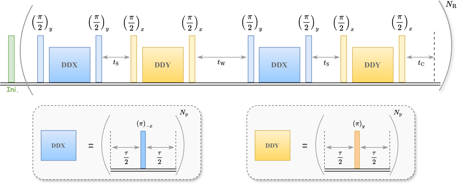
Figure 1: Hyper-polarization protocol of nuclear spins. The green box denotes the initialization process of the electron spin. After the initialization, the electron experiences two identical unitary processes($\mathrm{DDX}$+$\mathrm{DDY}$) separated by a waiting time $t_{\mathrm{W}}$. There is also a delay $t_{\mathrm{S}}$ between $\mathrm{DDX}$ and $\mathrm{DDY}$, which represents the DD process under different $\pi$ pulses as shown in the graphs below. Here $N_{\mathrm{p}}$ denotes the pulse number of DD process.

II.1 Kraus operator form for hyper-polarization

We consider that an electron spin(denoted by spin operator $\hat{\mathbf{S}}$) interacts with the nuclear spin(denoted by spin operator $\hat{\mathbf{I}}$) via the hyperfine coupling. The Hamiltonian can always be written in the standard form

$$\hat{H}=\omega\hat{I}_{z}+\hat{S}_{z}\mathbf{A}\cdot\hat{\mathbf{I}},$$ (1)

in the rotation frame of electron spin when choosing a suitable coordinate of nuclear spin. Here $\omega$ denotes the effective Larmor frequency of the nuclear spin[46]. When choosing a proper $x$ axis of the nuclear spin, the hyperfine tensor can be written to $\mathbf{A}\equiv\{A_{\bot},0,A_{z}\}$ with $y$ component vanishing[46].

The proposed Hyper-polarization protocol is shown in Fig.1, which includes $N$ units. In each unit, there are eight steps shown as following:

1. Electron spin initialization: The electron spin is firstly initialized to the state $|\Uparrow\rangle$, for example, by laser illumination in NV center[14];

2. DDX: DD sequence(with the $\pi$ pulse around $-x$ axis, see Fig. 1) with $\pi$ pulse number $N_{\mathrm{p}}$ and pulse interval $\tau$, sandwiched by two half $\pi$ pulse around $y$ axis is applied. In principle, the axis of $\pi$ pulse can be any direction in the $x-y$ plane;

3. Waiting for a duration $t_{\mathrm{S}}$ : The nuclear spin evolves freely without hyperfine coupling, which can be realized by DD sequence with pulse interval unresonant with the nuclear spin[37];

4. DDY: Another DD sequence(with the $\pi$ pulse around $y$ axis, see Fig. 1) sandwiched by two half $\pi$ pulse around $x$ axis is applied;

5. Waiting for a duration $t_{\mathrm{W}}$ : Another waiting process with duration $t_{\mathrm{W}}$ is implemented. In this process, the nuclear spin also evolves freely as the Step.3;

6. Step. 2-Step. 4 is repeated again;

7. Another waiting time $t_{\mathrm{C}}$ to compensate for the phase difference;

8. Step.2-Step. 7 is repeated for $N_{\mathrm{R}}$ times.

The total unitary evolution of the total electron-nuclear spin system is described by the unitary operation $\hat{U}$ (see details in the Appendix. A).

Then we use the unitary operation $\hat{U}$ to formulate the polarization process clearly. After the initialization process(Step. 1), the density matrix of the nuclear spin and electron spin can always be described by a separated state $\hat{\rho}=|\Uparrow\rangle\langle\Uparrow|\otimes\hat{\rho}_{\mathrm{N}}$ due to the initialization of electron spin. Denoting $\hat{\rho}_{\mathrm{N}}^{(n)}$ as the density matrix of the nuclear spin after the $n$th initialization, the evolution of the nuclear spin state can be described by the recursion equation

$$\hat{\rho}_{\mathrm{N}}^{(n+1)}=\mathcal{M}\hat{\rho}_{\mathrm{N}}^{(n)},$$ (2)

where the super-operator $\mathcal{M}$ is defined as

$$\mathcal{M}\hat{\rho}_{\mathrm{N}}\equiv\mathrm{Tr}_{\mathrm{S}}\left[\hat{U}\left(|\Uparrow\rangle\langle\Uparrow|\otimes\hat{\rho}_{\mathrm{N}}\right)\hat{U}^{\dagger}\right],$$ (3)

where $\mathrm{Tr}_{\mathrm{S}}$ denotes the trace over freedom of electron spin. Inserting the completeness $|\Uparrow\rangle\langle\Uparrow|+|\Downarrow\rangle\langle\Downarrow|=1$ to the formula above, the super-operator $\mathcal{M}$ can be reformulated to

$$\mathcal{M}\hat{\rho}_{\mathrm{N}}=\hat{M}_{\Uparrow}\hat{\rho}_{\mathrm{N}}\hat{M}_{\Uparrow}^{\dagger}+\hat{M}_{\Downarrow}\hat{\rho}_{\mathrm{N}}\hat{M}_{\Downarrow}^{\dagger},$$ (4)

by using the Kraus operators $\hat{M}_{\Uparrow}=\langle\Uparrow|\hat{U}|\Uparrow\rangle$ and $\hat{M}_{\Downarrow}=\langle\Downarrow|\hat{U}|\Uparrow\rangle$ . Then the dynamics of the hyper-polarization of nuclear spin can be simulated directly by Eq. (2).

II.2 Approximated Analytical Result

After the first order Magnus expansion, the evolution operator of each unit $\hat{U}$[Eq. (18)] can be approximated to the following standard form(see Appendix. A)

$$\hat{U}\approx-e^{-iN_{\mathrm{R}}\Phi\hat{I}_{z}}\exp\left\{-i\alpha\left(\hat{S}_{x}\mathbf{e}_{\mathrm{X}}\cdot\hat{\mathbf{I}}+\hat{S}_{y}\mathbf{e}_{\mathrm{X},\phi}\cdot\hat{\mathbf{I}}\right)\right\},$$ (5)

where the phase $\Phi=\omega T$ is precessing angle of the nuclear spin during single unit of the $N_{\mathrm{R}}$ repetitions of the protocol[Fig. 1] and $T\equiv 2t_{\mathrm{S}}+t_{\mathrm{W}}+4N_{\mathrm{p}}\tau+t_{\mathrm{C}}$ is corresponding duration. $\mathbf{e}_{\mathrm{X}},\mathbf{e}_{\mathrm{Y}}$ are two properly chosen unit vectors perpendicular to each other, which depends on the detail of control parameters(see Appendix. A). $\mathbf{e}_{\mathrm{X},\phi}$ is a unit vector $\mathbf{e}_{\mathrm{X},\phi}=\cos\phi\mathbf{e}_{\mathrm{X}}+\sin\phi\mathbf{e}_{\mathrm{Y}}$ and $\phi$ is an angle depends on the time sequence

$$\phi=\frac{(-1)^{N_{\mathrm{p}}}+1}{2}\pi-\omega\left(t_{\mathrm{S}}+N_{\mathrm{p}}\tau\right),$$ (6)

[modulus by $2\pi$] and $\alpha$ is a real parameter defined as following

$$\alpha=2A_{\bot}\frac{\sin\left(N_{\mathrm{R}}\Phi/2\right)}{\sin\left(\Phi/2\right)}\sin\frac{\Phi_{1}}{2}F(\omega,N_{\mathrm{p}},\tau),$$ (7)

whose absolute quantify the efficiency of the polarization protocol. Here $\Phi_{1}=\omega\left(t_{\mathrm{S}}+t_{\mathrm{W}}+2N_{\mathrm{p}}\tau\right)$ is the precessing phase of the nuclear spin between the first DDX and the second DDX and $F(\omega,N_{\mathrm{p}},\tau)$ is

$$F(\omega,N_{\mathrm{p}},\tau)=\begin{cases}-\frac{4\sin\left(\frac{N_{\mathrm{p}}\omega\tau}{2}\right)\sin^{2}\left(\frac{\omega\tau}{4}\right)}{\omega\cos\left(\frac{\omega\tau}{2}\right)}&\mathrm{mod}\left(N_{\mathrm{p}},2\right)=0\\ \frac{4\cos\left(\frac{N_{\mathrm{p}}\omega\tau}{2}\right)\sin^{2}\left(\frac{\omega\tau}{4}\right)}{\omega\cos\left(\frac{\omega\tau}{2}\right)}&\mathrm{mod}\left(N_{\mathrm{p}},2\right)=1,\end{cases}$$

In Eq. (7), the first factor $\sin\left(N_{\mathrm{R}}\Phi/2\right)/\sin\left(\Phi/2\right)$ quantifies the synchronization between each evolution unit, the second factor $\sin\left(\Phi_{1}/2\right)$ quantifies the synchronization between the two DDX-DDY sequences in Fig. 1 and the third factor $F(\omega,N_{\mathrm{p}},\tau)$ quantifies the resonance between the DD pulse interval and the Larmor frequency of the nuclear spin[47, 46].

Using the approximation in Eq. (5), the Kraus operator Eq. (4) can be calculated analytically to be

$$\hat{M}_{\Uparrow}= -\left(\begin{matrix}e^{-i\frac{\Phi}{2}}\cos\left(\alpha\cos\theta/2\right)&0\\ 0&e^{i\frac{\Phi}{2}}\cos\left(\alpha\sin\theta/2\right)\end{matrix}\right)$$ (8)

$$\hat{M}_{\Downarrow}= \left(\begin{matrix}0&-e^{-i\left(\theta+\frac{\Phi}{2}\right)}\sin\left(\alpha\sin\theta/2\right)\\ ie^{i\left(\theta+\frac{\Phi}{2}\right)}\sin\left(\alpha\cos\theta/2\right)&0\end{matrix}\right),$$

in the basis of $|\uparrow\rangle$ and $|\downarrow\rangle$ of nuclear spin basis and $\theta$ is an angle defined as $\theta=\phi/2+\pi/4$. The Kraus operator in Eq. (8) can be used to investigate analytically the polarization dynamics.

III Result

III.1 Optimal working point

Table 1: The magic numbers for the Method.I and Method.II. The unit of the parameters $\tau$ and $t_{\mathrm{S}},t_{\mathrm{W}},t_{\mathrm{C}}$ are set to $\pi/\omega$. The left are the optimized parameters of Method.I while the right are that of Method.II. If $N_{\mathrm{R}}=1$, $t_{\mathrm{C}}=0$ while for other cases, $t_{\mathrm{C}}$ takes the value in this table. The polarization window $\Gamma$[in unit of $\omega/(N_{\mathrm{R}}\pi)$] and side bands $\delta\omega_{\mathrm{side}}$(in unit of $\pi/\omega$)of these two methods are also listed in this table.

	Method.I					Method.II
( $P_{\mathrm{s}}$, $N_{\mathrm{p}}$)	$\tau$[$\pi/\omega$]	$t_{\mathrm{S}},t_{\mathrm{W}},t_{\mathrm{C}}$[$\pi/\omega$ mod($2\pi/\omega$)]	$\Gamma$[ $\frac{\omega}{N_{\mathrm{R}}\pi}$]	$\delta\omega_{\mathrm{side}}[\pi/\omega]$	( $P_{\mathrm{s}}$, $N_{\mathrm{p}}$)	$\tau$[$\pi/\omega$]	$t_{\mathrm{S}},t_{\mathrm{W}},t_{\mathrm{C}}$[$\pi/\omega$]	$\Gamma$[ $\frac{\omega}{N_{\mathrm{R}}\pi}$]	$\delta\omega_{\mathrm{side}}$[$\pi/\omega$ mod($2\pi/\omega$)]
$+1,N_{\mathrm{p}}=1$	$2$	$3/2$	$2/7$	$\pm 2k/7$	$+1,N_{\mathrm{p}}=1$	$3/2$	$0$	$1/3$	$\pm 2k/3$
$-1,N_{\mathrm{p}}=1$	$2$	$1/2$	$2/5$	$\pm 2k/5$	$-1,N_{\mathrm{p}}=1$	$5/2$	$0$	$1/5$	$\pm 2k/5$
$+1,N_{\mathrm{p}}=2$	$4/3$	$11/6$	$2/9$	$\pm 2k/9$	$+1,N_{\mathrm{p}}=2$	$5/4$	$0$	$2/5$	$\pm 2k/5$
$-1,N_{\mathrm{p}}=2$	$4/3$	$5/6$	$2/7$	$\pm 2k/7$	$-1,N_{\mathrm{p}}=2$	$11/4$	$0$	$2/11$	$\pm 2k/11$
$+1$, $N_{\mathrm{p}}\geq 3$	$1$	$1/2$	$2/(2N_{\mathrm{p}}+1)$	$\pm 2k/(2N_{\mathrm{p}}+1)$	$+1$, $N_{\mathrm{p}}\geq 3$	$1+\frac{1}{2N_{\mathrm{p}}}$	$0$	$2/(2N_{\mathrm{p}}+1)$	$\pm 2k/(2N_{\mathrm{p}}+1)$
$-1,$ $N_{\mathrm{p}}\geq 3$	$1$	$3/2$	$2/(2N_{\mathrm{p}}+3)$	$\pm 2k/(2N_{\mathrm{p}}+3)$	$-1,$ $N_{\mathrm{p}}\geq 3$	$1-\frac{1}{2N_{\mathrm{p}}}$	$0$	$2/(2N_{\mathrm{p}}-1)$	$\pm 2k/(2N_{\mathrm{p}}-1)$

Before going to analyze in detail the performance from the Kraus operator in Eq. (8), we first give an intuitive analysis of stable polarization from the effective evolution operator in Eq. (5). From Eq. (5), the phase $\phi$[Eq. (6)] is obviously an important parameter which controls the stable polarization since it decides the form of the effective Hamiltonian. To make the polarization degree perfect, we need to set the phase $\phi$ to half integer of $\pi$[see Eq. (6)], namely

$$\phi=\begin{cases}\frac{\pi}{2},\mathrm{perfect}\ \mathrm{positive}\ \mathrm{polarization}\\ \frac{3\pi}{2},\mathrm{perfect}\ \mathrm{negative}\ \mathrm{polarization}\end{cases},$$ (9)

(modulus $2\pi$). For example, if $\phi$ is equal to $\pi/2$, then we have $\mathbf{e}_{\mathrm{X},\phi}=\mathbf{e}_{\mathrm{Y}}$ and hence exponent of Eq. (5) has form $\hat{S}_{+}\hat{I}_{-}+\hat{S}_{-}\hat{I}_{+}$, which leads to full positive polarization. However, if the phase $\phi$ is tuned to $3\pi/2$, then we have $\mathbf{e}_{\mathrm{X},\phi}=-\mathbf{e}_{\mathrm{Y}}$ and hence exponent of Eq. (5) has form $\hat{S}_{+}\hat{I}_{+}+\hat{S}_{-}\hat{I}_{-}$, which leads to full negative polarization.

To optimize the polarization performance, we need keep the perfect polarization condition Eq. (9) while simultaneously maximizing $\alpha$ in Eq. (7). These parameters are called optimal working point. There are two methods to achieve the optimal working point. One method[called Method.I] is maximizing $\alpha$ by tuning the three parameters $t_{\mathrm{S}},t_{\mathrm{W}},t_{\mathrm{C}}$ independently while simultaneously keeping the perfect polarization. This is equal to maximizing the three factors of Eq. (7) respectively. So we need to set $\Phi$ to be $2k\pi$, $\Phi_{1}$ to be $(2k+1)\pi$[see Eq. (7)] and $\tau$ to be resonant to nuclear spin[see Eq. (7) and Table. 2 in the Appendix] while simultaneously fixing $\phi$ be half integer[Eq. (9)]. The other method[called Method.II] is maximizing $\alpha$ only by tuning $\tau$ when fixing $t_{\mathrm{S}}=t_{\mathrm{W}}=t_{\mathrm{C}}=0$ and simultaneously keeping the perfect polarization[$\phi$ be half integer[Eq. (9)]. In this case, there is only one parameter $\tau$ can be tuned. The magic parameters for Method.I are shown in the left Table.1 while the Method.II in the right Table.1 after detailed analysis in the Appendix.C.1 and Appendix.C.2.

III.2 Stable polarization

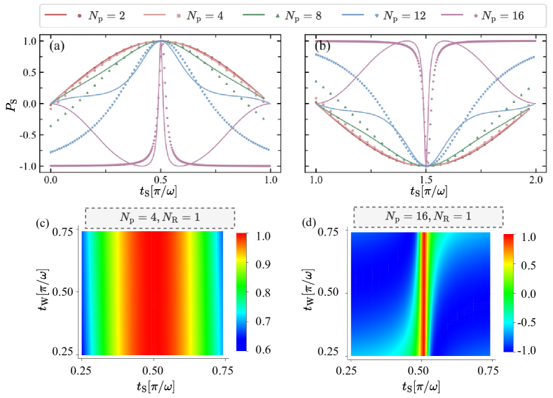
Figure 2: Stable polarization vs waiting time. The stable polarization as a function of $t_{\mathrm{S}}$ for the case of (a) $N_{\mathrm{R}}=1$, $t_{\mathrm{W}}=t_{\mathrm{C}}=\pi/(2\omega)$, $N_{\mathrm{p}}=2$(red), $N_{\mathrm{p}}=4$(brown), $N_{\mathrm{p}}=8$(green), $N_{\mathrm{p}}=12$(blue) and $N_{\mathrm{p}}=16$(purple). (b) $N_{\mathrm{R}}=1$, $t_{\mathrm{W}}=t_{\mathrm{C}}=3\pi/(2\omega)$, $N_{\mathrm{p}}=2$(red), $N_{\mathrm{p}}=4$(brown), $N_{\mathrm{p}}=8$(green), $N_{\mathrm{p}}=12$(blue) and $N_{\mathrm{p}}=16$(purple). The scatters are the numerically simulated results while the lines with the same color are the corresponding analytical results; The stable polarization as a function of both $t_{\mathrm{S}},t_{\mathrm{W}}$ for the case of (c) $N_{\mathrm{p}}=4,N_{\mathrm{R}}=1$ (d) $N_{\mathrm{p}}=16,N_{\mathrm{R}}=1$. For all these graphs, the parameters of the Hamiltonian are $A_{\perp}=0.1,\omega=1$.

In the following, we analyze quantitatively the stable polarization from the dynamical equation[Eq. (2)] and approximated Kraus operator[Eq. (8)]. If we only focus on the polarization, we can neglect the coherence of the nuclear spin and the density matrix can be written as $\hat{\rho}_{\mathrm{N}}^{(N-1)}=P_{\uparrow}^{(N-1)}|\uparrow\rangle\langle\uparrow|+P_{\downarrow}^{(N-1)}|\downarrow\rangle\langle\downarrow|$ after the $N$th initialization($P_{\uparrow/\downarrow}^{(N)}$ is the population of the nuclear state $|\uparrow/\downarrow\rangle$). Inserting this equation to the Eq. (2) and using the approximated expression of the Kraus operator Eq. (8), we obtain the recursion equation for the nuclear spin population

$$\left(\begin{array}[]{c}P_{\uparrow}^{(N+1)}\\ P_{\downarrow}^{(N+1)}\end{array}\right)=\left(\begin{matrix}\cos^{2}\left(\frac{\alpha\cos\theta}{2}\right)&\sin^{2}\left(\frac{\alpha\sin\theta}{2}\right)\\ \sin^{2}\left(\frac{\alpha\cos\theta}{2}\right)&\cos^{2}\left(\frac{\alpha\sin\theta}{2}\right)\end{matrix}\right)\left(\begin{array}[]{c}P_{\uparrow}^{(N)}\\ P_{\downarrow}^{(N)}\end{array}\right).$$ (10)

Using this equation, the stable polarization $P_{\mathrm{s}}\equiv P_{\uparrow}^{(+\infty)}-P_{\downarrow}^{(+\infty)}$ is calculated analytically to be

$$P_{\mathrm{s}}=\frac{\sin^{2}\left(\frac{1}{2}\alpha\sin\theta\right)-\sin^{2}\left(\frac{1}{2}\alpha\cos\theta\right)}{\sin^{2}\left(\frac{1}{2}\alpha\sin\theta\right)+\sin^{2}\left(\frac{1}{2}\alpha\cos\theta\right)},$$ (11)

The stable polarization can be controlled by the parameter $\phi$ from the analytical formula Eq. (11) since $\theta=\phi/2+\pi/4$. As shown in Eq. (6), the parameter $\phi$ can be controlled by the time delay $t_{\mathrm{S}}$ and DD parameters $N_{\mathrm{p}},\tau$[Eq. (6)] while is irrelevant to $t_{\mathrm{W}},t_{\mathrm{C}}$. At the optimal working, $\phi$ is equal to half integer of $\pi$ and hence the stable polarization is perfect, which is independent of the quantity $\alpha$. Specifically, for $\phi=\pi/2$($\theta=\pi/2$)(modulus $2\pi$), Eq. (11) gives perfect positive polarization. For $\phi=3\pi/2$($\theta=\pi$)(modulus $2\pi$), however, Eq. (11) gives perfect negative polarization, which is consistent with the analysis from the form of the effective Hamiltonian in Eq. (5).

The stable polarization is highly sensitive to deviations in $t_{\mathrm{S}}$ when $\alpha$ is large. To validate these conclusions, we use the parameters $\tau=\pi/\omega$, $t_{\mathrm{S}}=t_{\mathrm{W}}=t_{\mathrm{C}}=\pi/(2\omega)$ and $\tau=\pi/\omega$, $t_{\mathrm{S}}=t_{\mathrm{W}}=t_{\mathrm{C}}=3\pi/(2\omega)$ of Method.I in Table 1 to generate perfect positive and negative polarization, respectively. By varying $t_{\mathrm{S}}$, we plot the stable polarization for these two cases in Fig. 2(a) and (b) while keep other parameters unchanged. Our results demonstrate that the stable polarization varies significantly as a function of $t_{\mathrm{S}}$, particularly for large $N_{\mathrm{p}}$. This behavior arises because a large $\alpha$ enhances the sensitivity of stable polarization to $\sin\theta$, and consequently to $t_{\mathrm{S}}$, as indicated by the analytical formula in Eq. (11). Although Eq. (11) loses accuracy for large $\alpha$ when $\phi$ deviates from the optimal working point defined in Eq. (9), it still captures the qualitative trends of stable polarization as a function of $t_{\mathrm{S}}$, as illustrated in Fig. 2(a) and (b).

The stable polarization is insensitive to the deviation of the other two waiting times $t_{\mathrm{W}},t_{\mathrm{C}}$. We plot the stable polarization as a function of both $t_{\mathrm{S}},t_{\mathrm{W}}$ in Fig. 2 (c) $N_{\mathrm{p}}=4$ and (d) $N_{\mathrm{p}}=16$. As shown in these figures, the stable polarization shows obvious dependence on $t_{\mathrm{S}}$ while nearly independent on $t_{\mathrm{W}}$. This can be roughly understood as following: When deviate from the optimal working point, $|\alpha|$ becomes very small and hence we can approximate the stable polarization as $P_{\mathrm{s}}\approx(\sin\theta-\cos\theta)/(\sin\theta+\cos\theta)$ from Eq. (11). Consequently, the stable polarization depends very weakly on $t_{\mathrm{W}},t_{\mathrm{C}}$ since $\theta$ is independent of $t_{\mathrm{W}},t_{\mathrm{C}}$.

III.3 Polarization Rate

The polarization rate of the nuclear spin is a key parameter to characterize the performance of the super-polarization protocol. It can be obtained by calculation of the dynamics of the polarization, which can be obtained by solving the dynamics equation Eq. (10). The result is

$$P^{(N)}=P_{\mathrm{s}}(1-\lambda^{N-1}),$$ (12)

if the initial state of the nuclear spin is taken to the complete mixed states(vanishing initial polarization). Here $\lambda$

$$\lambda=\frac{1}{2}\left|\cos\left(\alpha\sin\theta\right)+\cos\left(\alpha\cos\theta\right)\right|,$$ (13)

is a quantity satisfying $\lambda\leq 1$. Under the optimal working point($\theta=\pi/2$ and $\theta=\pi$), we have $\lambda=\cos^{2}(\alpha/2)$. Using $\lambda$, we can define $N_{\mathrm{s}}=\max\left\{-1/\ln\lambda,1\right\}$(the number $1$ comes from the fact that the repetitive times can not be smaller than $1$) to characterize the typical repetitive times to polarize the nuclear spin(where $N_{\mathrm{s}}$ is defined as $P^{(N_{\mathrm{s}})}/P_{\mathrm{s}}=1-e^{-1}$). Then the typical polarization time can be defined as $T_{1}=N_{s}N_{\mathrm{R}}T$ and the polarization rate is then defined as $\gamma=1/T_{1}$

$$\gamma=\frac{\min\left\{-\ln\lambda,1\right\}}{N_{\mathrm{R}}T}.$$ (14)

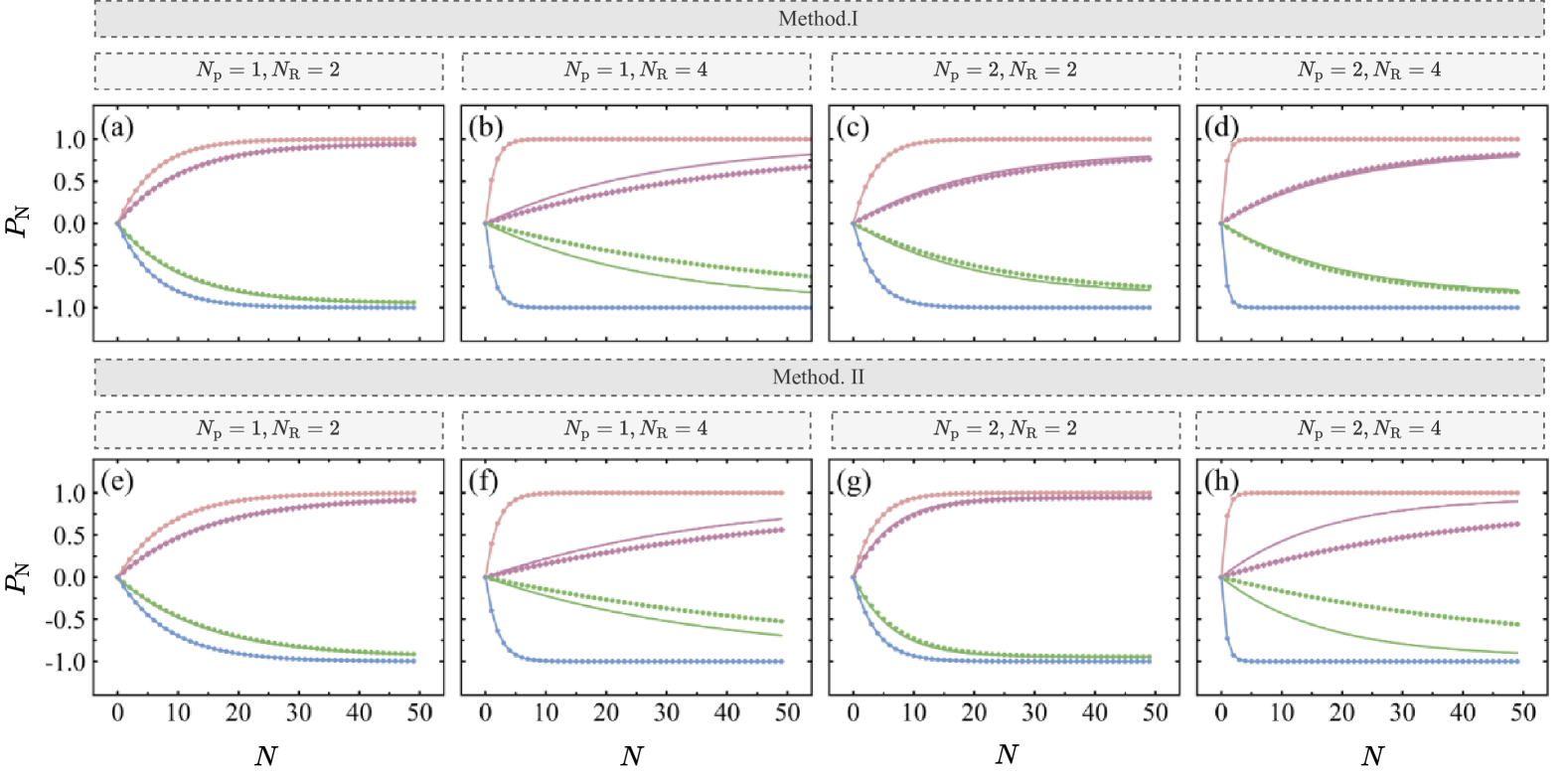
Figure 3: Polarization dynamics. $P_{N}$ as a function of repetitive times $N$. The Scatters are the numerically simulated results while the line with the same color are the corresponding analytical result. The blue and pink scatters and line are the results for perfect positive and negative polarization respectively with the parameters taken from the left of Table. 1. The other cases are the parameters $t_{\mathrm{S}},t_{\mathrm{W}},t_{\mathrm{C}}$ with small deviation from these ideal parameters. Specifically, the graphs above plot the Method.I when (a) $N_{\mathrm{p}}=1,N_{\mathrm{R}}=2$. (b) $N_{\mathrm{p}}=1,N_{\mathrm{R}}=4$. (c) $N_{\mathrm{p}}=2,N_{\mathrm{R}}=2$. (d) $N_{\mathrm{p}}=2,N_{\mathrm{R}}=4$. $t_{\mathrm{S}}=t_{\mathrm{W}}=t_{\mathrm{C}}=2.8\pi/(2\omega)$(purple), $t_{\mathrm{S}}=t_{\mathrm{W}}=t_{\mathrm{C}}=1.2\pi/(2\omega)$(green) for $N_{\mathrm{p}}=1$ while $t_{\mathrm{S}}=t_{\mathrm{W}}=t_{\mathrm{C}}=10\pi/(6\omega)$(purple), $t_{\mathrm{S}}=t_{\mathrm{W}}=t_{\mathrm{C}}=\pi/\omega$(green) for $N_{\mathrm{p}}=2$. The graphs below plot the Method.II when (a) $N_{\mathrm{p}}=1,N_{\mathrm{R}}=2$. (b) $N_{\mathrm{p}}=1,N_{\mathrm{R}}=4$. (c) $N_{\mathrm{p}}=2,N_{\mathrm{R}}=2$ and (d) $N_{\mathrm{p}}=2,N_{\mathrm{R}}=4$. The parameters are $t_{\mathrm{S}}=t_{\mathrm{W}}=t_{\mathrm{C}}=0$ for red and blue data while $t_{\mathrm{S}}=t_{\mathrm{W}}=t_{\mathrm{C}}=0.1\pi/\omega$ for the green and purple data. For all these figures, $\omega=1$ and $A_{\perp}=0.05,A_{z}=0$.

To demonstrate the analytical result[Eq. (12)] of the polarization dynamics, we compare it with that of the numerical simulated result in Fig. 3 for the parameters in Table. 1. They are consistent with each other very well for perfect polarization while only qualitatively consistent when $\phi$ deviates from the optimal working point in Table. 1.

There is an approximated formula for polarization rate for weakly coupled nuclear spin($A_{\perp}\ll\omega$) under optimal working point. For weakly coupled nuclear spin, using the parameters in Table. 1, the polarization rate for the two methods under the case of perfect polarization can be approximated to

$$\gamma_{\mathrm{opt}}\approx\frac{A_{\bot}}{\pi}\min\left\{\frac{-\ln\cos\left(\alpha_{\mathrm{max}}/2\right)}{\alpha_{\mathrm{max}}/2},\frac{1}{\alpha_{\mathrm{max}}}\right\},$$ (15)

by noting that it requires large pulse number $N_{\mathrm{p}}$ for weakly coupled case and hence the time cost in each unit is largely spent in the duration of DD sequence. Here $\alpha_{\mathrm{max}}=4N_{\mathrm{R}}N_{\mathrm{p}}A_{\bot}/\omega$ is the maximal $\alpha$ which can be achieved for fixed $N_{\mathrm{R}}N_{\mathrm{p}}$[see Eq. (7)].

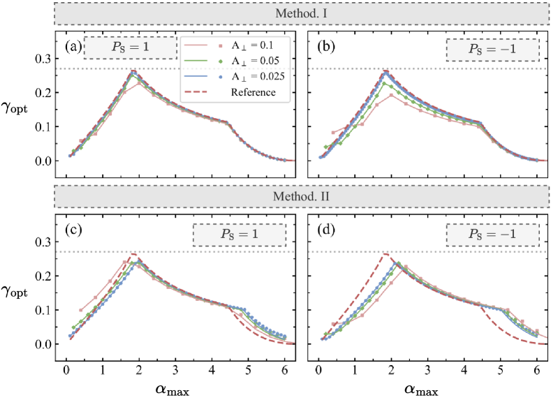
Figure 4: Polarization rate[in unit of $2A_{\bot}/\pi$] vs $N_{\mathrm{p}}$. $\gamma$ as a function of $\alpha_{\mathrm{max}}$ as $N_{\mathrm{p}}$ increases when $N_{\mathrm{R}}=1$ is fixed. (a) Method. I when $P_{\mathrm{s}}=1$. (b) Method.I when $P_{\mathrm{s}}=-1$. (c) Method.II when $P_{\mathrm{s}}=1$. (d) Method.II method when $P_{\mathrm{s}}=-1$. The pink, green and blue data represent the case of $A_{\bot}=0.1$, $A_{\bot}=0.05$ and $A_{\bot}=0.025$ respectively. The scatters are the numerically simulated results while the line with the same color are the corresponding analytical results. The red dashed linesis the reference line from the approximated formula Eq. (15) for weakly coupled limit. For all the figures, the Larmor frequency is set to $\omega=1$.

Under the optimal working point, the polarization rate shows an initial linear increasing as the $N_{\mathrm{p}},N_{\mathrm{R}}$ increase since the polarization rate $\gamma_{\mathrm{opt}}$ can be further approximated to

$$\gamma_{\mathrm{opt}}\approx\frac{A_{\bot}}{4\pi}\alpha_{\mathrm{max}}\approx N_{\mathrm{R}}N_{\mathrm{p}}\gamma_{0},$$ (16)

for small $\alpha_{\mathrm{max}}$($\alpha_{\mathrm{max}}\ll 1$). Here $\gamma_{0}$ is defined as $A_{\bot}^{2}/(\pi\omega)$. To prove this relation, we simulate $\gamma_{\mathrm{opt}}$ as a function of $\alpha_{\mathrm{max}}$ in Fig. 4 for both Method.I and Method.II under various parameters. In all these figures, $\gamma_{\mathrm{opt}}$ shows an initial linear increasing with respective to $\alpha_{\mathrm{max}}$. Besides, the consistent between the analytical formula Eq.(16) and the numerical result also enable us to measure the transverse coupling $A_{\bot}$ via the polarization dynamics.

As the $N_{\mathrm{p}}$ continue increasing, the optimal polarization rate will reach an universal maximal polarization rate $0.54A_{\bot}/\pi$ determined by the transverse hyperfine coupling $A_{\bot}$. From Eq. (15), the optimal polarization rate $\gamma_{\mathrm{opt}}$(in unit of $2A_{\bot}/\pi$) is a sole function of $\alpha_{\mathrm{max}}$ and arrives its maximum $0.27$ when $\alpha_{\mathrm{max}}\approx 1.84$. As a result, the maximum of $\gamma_{\mathrm{opt}}$ is $0.54A_{\bot}/\pi$ limited by the hyperfine coupling $A_{\bot}$. As shown in Fig. 4, we plot $\gamma_{\mathrm{opt}}$ (in unit of $2A_{\bot}/\pi$) for both two methods as a function of $\alpha_{\mathrm{max}}$ as the $N_{\mathrm{p}}$ is changed. As the coupling $A_{\bot}$ decreases from $A_{\bot}=0.1$(pink scatters in Fig. 4) to $A_{\bot}=0.025$(blue scatters in Fig. 4), the numerical result of $\gamma_{\mathrm{opt}}$ gradually converges to reference line set by the approximated formula[Eq. (15)] and shows an universal maximum $0.27$(in unit of $2A_{\bot}/\pi$) for both the Method.I and Method.II.

III.4 The effect of finite pulse duration

In realistic polarization protocol, the duration of the half $\pi$ pulse can never be zero[see Fig. 1] and is usually limited by the micro wave power. As a result, we need consider how the duration of the half $\pi$ pulse affects the polarization performance of the methods in Table. 1. For realistic polarization protocol in NV center, the typical pulse duration $\tau_{\mathrm{\pi}}$ of the $\pi$ pulse is about $50\mathrm{ns}$(duration of half $\pi$ pulse is $\tau_{\mathrm{\pi}}/2$) and the typical Larmor frequency is about $\omega\sim 2\pi\times 1\mathrm{MHz}$ for ${}^{13}\mathrm{C}$[46, 37] and $\omega\sim 2\pi\times 4\mathrm{MHz}$ for ${}^{1}\mathrm{H}$ under the magnetic field $0.1\mathrm{T}$. Consequently, the maximum $\tau_{\mathrm{\pi}}$ can reach up to $0.4\pi/\omega$ and hence can not been neglected under strong magnetic field or for nuclear spin with large gyromagnetic ratio.

Firstly, we investigate how the pulse duration affects the optimal working point shown in Table. 1. We keep all the waiting times $t_{\mathrm{W}},t_{\mathrm{S}},t_{\mathrm{C}}$ unchanged, the modified $\tilde{\tau}$ should be shift to

$$\tilde{\tau}=\tau_{\mathrm{ideal}}-\frac{\tau_{\mathrm{\pi}}}{N_{\mathrm{p}}},$$ (17)

due to the existence of finite duration of half $\pi$ pulse, where $\tau_{\mathrm{ideal}}$ is the ideal value in Table.1. This formula is testified by numerical simulation shown in Fig.5(a). We simulate the finite pulse duration by adding a Rabi term with Rabi frequency be $\Omega=\pi/\tau_{\mathrm{\pi}}$ and then numerically calculate the $\tau=\tau_{\mathrm{res}}$ which maximized the polarization rate $\gamma$. We plot the optimized $\tau_{\mathrm{res}}$ as a function of $\tilde{\tau}$ for various $\omega$ and $\tau_{\mathrm{\pi}}$ in Fig.5(a). They are equal to each other as shown by the reference line in Fig.5(a) and hence the optimized value in Eq. (17) is proved to be correct.

Then we show the advantage of our new protocol over the PulsePol protocol in Ref. [20]. To do this, we compare the robustness of various protocol in Table.1 to the duration $\tau_{\mathrm{\pi}}$ under the modified optimal working point[Eq. (17)]. We focus on the the first parameters $N_{\mathrm{p}}=1,t_{\mathrm{S}}=t_{\mathrm{W}}=t_{\mathrm{S}}=0$ of the Method.II in Table. 1[essentially the PulsePol protocol in Ref. [20]] and the first two parameters of Method.I in Table. 1. To do a relative fair comparison, we tune the optimized polarization rate to be nearly the same for these three parameters under infinite short $\tau_{\mathrm{\pi}}$(infinite large Rabi frequency). This leads to the parameters $N_{\mathrm{p}}=1,N_{\mathrm{R}}=13,t_{\mathrm{S}}=t_{\mathrm{W}}=t_{\mathrm{S}}=3\pi/(2\omega)$, $N_{\mathrm{p}}=1,N_{\mathrm{R}}=10,t_{\mathrm{S}}=t_{\mathrm{W}}=t_{\mathrm{S}}=\pi/(2\omega)$ and $N_{\mathrm{p}}=1,N_{\mathrm{R}}=8,t_{\mathrm{S}}=t_{\mathrm{W}}=t_{\mathrm{S}}=0$. Then we calculate the stable polarization degree $|P_{\mathrm{s}}|$ and polarization rate $\gamma_{\mathrm{opt}}$ under the optimal working point as a function of $\tau_{\mathrm{\pi}}$[in unit of $\pi/\omega$]. These results are shown in Fig. 5 (b). We can see that both the two new methods[$N_{\mathrm{p}}=1,N_{\mathrm{R}}=13,t_{\mathrm{S}}=t_{\mathrm{W}}=t_{\mathrm{S}}=3\pi/(2\omega)$ and $N_{\mathrm{p}}=1,N_{\mathrm{R}}=10,t_{\mathrm{S}}=t_{\mathrm{W}}=t_{\mathrm{S}}=\pi/(2\omega)$] proposed in this paper show obvious robustness over the PulsePol protocol in Ref. [20][the parameter $N_{\mathrm{p}}=1,N_{\mathrm{R}}=8,t_{\mathrm{S}}=t_{\mathrm{W}}=t_{\mathrm{S}}=0$]. We also plot the polarization dynamics of $|P_{\mathrm{s}}|$ for various pulse duration $\tau_{\mathrm{\pi}}$[in unit of $\pi/\omega$]. We can see the dynamics of both the two new methods show obvious robustness to $\tau_{\mathrm{\pi}}$ over that of PulsePol.

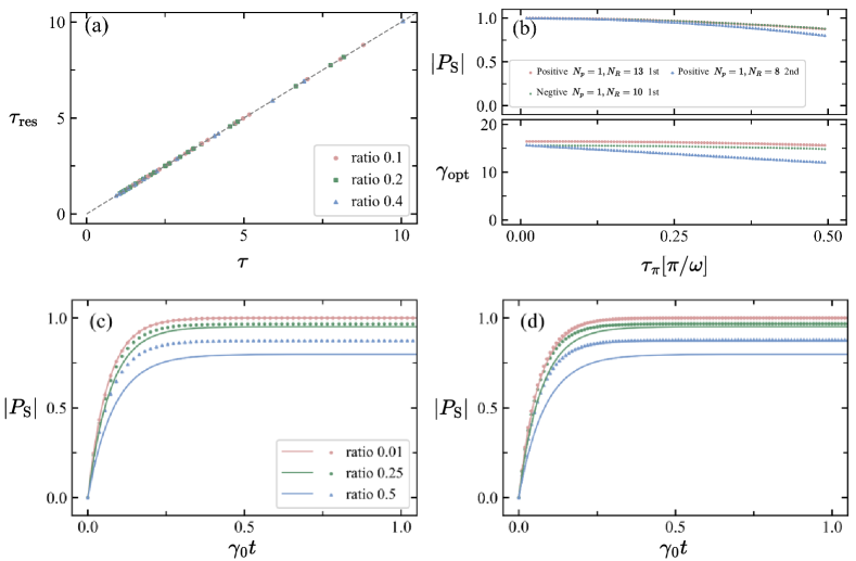
Figure 5: The effect of finite pulse duration. (a) The numerically searched $\tau_{\mathrm{res}}$ maximizing the polarization rate as a function of theoretical value $\tilde{\tau}$ modified by finite pulse duration as shown in Eq. (17). The black dashed line is the reference line $\tau_{\mathrm{res}}=\tilde{\tau}$. Numerical results are calculated for Method.I($N_{\mathrm{p}}=1,N_{\mathrm{R}}=8$ and $N_{\mathrm{p}}=2,N_{\mathrm{R}}=4$) and Method.II($N_{\mathrm{p}}=1,N_{\mathrm{R}}=8$) under the case of $\tau_{\mathrm{\pi}}=0.1\pi/\omega$[red dot], $0.2\pi/\omega$[green dot],$0.4\pi/\omega$[blue dot] when $\omega$ is changed from $0.5$ to $4$. (b) The absolute value of the stable polarization(graph above) and polarization rate $\gamma$(graph below) as a function of pulse duration $\tau_{\mathrm{\pi}}$[in unit of $\pi/\omega$]. The parameters are: red dot(positive polarization case of Method.I when $N_{\mathrm{p}}=1,N_{\mathrm{R}}=13$ in Table. 1), green dot(negative polarization case of Method.I when $N_{\mathrm{p}}=1,N_{\mathrm{R}}=10$ in Table. 1) and blue dot(positive polarization case of Method.II when $N_{\mathrm{p}}=1,N_{\mathrm{R}}=8$ in Table. 1). The Larmor is all set to $\omega=1$. (c), (d) The comparison of the polarization dynamics between Method.I and PulsePol method(positive case of $N_{\mathrm{p}}=1$ of Method.II in Table. 1) when $\tau_{\mathrm{\pi}}=0.5\pi/\omega$. The other parameters is the same to (b). In graph (c) and (d) we compare the polarization dynamics of the first parameter ($N_{\mathrm{p}}=1,N_{\mathrm{R}}=13$), the second parameter($N_{\mathrm{p}}=1,N_{\mathrm{R}}=10$ ) of Method.I and that of PulsePol method respectively. Red, blue, green solid lines are the results of PulsePol method while the corresponding dashed line are that of Method.I. For all these figures, the coupling is set to $A_{\perp}=0.01$.

III.5 The polarization window and side bands

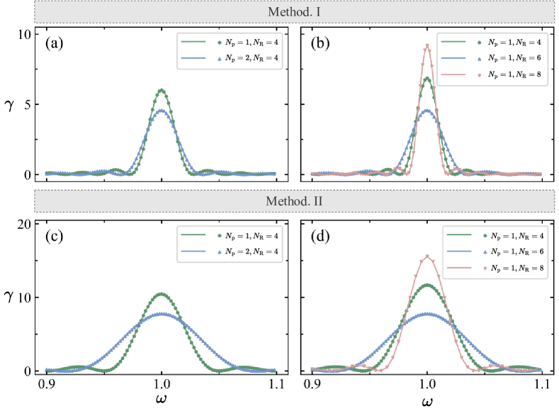
Figure 6: The polarization window for Method.I and Method.II. The polarization rate[in unit of $\gamma_{0}\equiv A_{\bot}^{2}/(\pi\omega)$] as a function of $\omega$. The Method.I : (a) Varying $N_{\mathrm{p}}$ while fixing $N_{\mathrm{R}}$; (b) Varying $N_{\mathrm{R}}$ while fixing $N_{\mathrm{p}}$. The Method.II: (c) Varying $N_{\mathrm{p}}$ while fixing $N_{\mathrm{R}}$. (d) Varying $N_{\mathrm{R}}$ fixing $N_{\mathrm{p}}$ . For all the figures, the Larmor frequency is set to $\omega=1$ and $A_{\perp}=0.005$. The other parameters are taken from the Table.1 for different $N_{\mathrm{p}}$ and $N_{\mathrm{R}}$.

In the following, we discuss the polarization window and side bands of the polarization protocol. The polarization window $\delta\omega$ is defined as the frequency range in which the nuclear spins can be effectively polarized, which quantified sensitivity of the protocol to the error of Larmor frequency. While the side bands of the polarization protocol is the extra polarization peak which will cause unwanted polarization effect.

We find the polarization window is proportional $1/(N_{\mathrm{R}}T)$. Since the stable polarization depends on $\phi$ in Eq. (6) while the polarization rate depends on $\alpha$ in Eq. (7), the stable polarization is less sensitive to the change of $\omega$ than the polarization rate if $N_{\mathrm{R}}$ is not equal to $1$. As a result, the polarization window is determined by the sensitivity of the polarization rate with respective to $\omega$, which is estimated to be $\delta\omega=4/(N_{\mathrm{R}}T)$ at which the first factor $\sin\left(N_{\mathrm{R}}\Phi/2\right)/\sin\left(\Phi/2\right)$ of Eq. 7 decay to $\sin(2)/2\approx 0.45$ of its maximum value. As a result, the polarization window $\delta\omega$ can be decreased by $N_{\mathrm{p}}$ and $N_{\mathrm{R}}$ as shown in Fig. 6 for both Method.I and Method.II. Once the Larmor frequency $\delta\omega$ lies out this range, the polarization rate will dramatically decrease. The polarization window $\delta\omega$ for different magic sequences are calculated in the Table. 1.

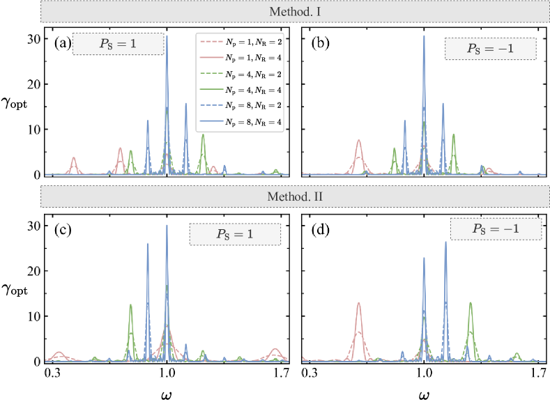
Figure 7: The side band of the polarization protocol. The polarization rate[in unit of $\gamma_{0}=A_{\bot}^{2}/(\pi\omega)$] is plot as a function of Larmor frequency $\omega$ when other parameters is fixed. The panel above shows the result of the Method.I when $P_{\mathrm{s}}$ is fixed to (a) $+1$ and (b) $-1$ for various pulse number $N_{\mathrm{p}}$ and $N_{\mathrm{R}}$, which is shown in the legend of the figures. The panel below shows the result of the Method.II when $P_{\mathrm{s}}$ is fixed to (c) $+1$ and (d) $-1$ for the same pulse number $N_{\mathrm{p}}$ and $N_{\mathrm{R}}$. For all the figures, we set $\tau=\pi/\omega_{0}$ and $A_{\perp}=0.005,A_{z}=0$. The other parameters take the value of Table. 1.

The position of the first side bands highly depends on $N_{\mathrm{p}}$ while nearly independent of $N_{\mathrm{R}}$. If we denote the side bands of the polarization rate by $\omega_{\mathrm{side}}$, the distant $\delta\omega_{\mathrm{side}}=\omega_{\mathrm{side}}-\omega$ from the central peak is calculated in the Table. 1 from Eq. (7). In Fig. 7, we plot the polarization rate as a function of $\omega$ under various $N_{\mathrm{p}},N_{\mathrm{R}}$ for both the two methods. As $N_{\mathrm{p}}$ increases, the sides bands will be closer to the central peak $\omega$ as shown in Fig. 7[see different colors and the same line shapes]. However, the side bands is nearly unchanged when $N_{\mathrm{R}}$ is increased while keeping $N_{\mathrm{p}}$ invariant[see different line shapes while the same colors in Fig. 7]. Since the side band will cause some unwanted effect, $N_{\mathrm{p}}$ should not be too large.

IV Conclusion and Outlook

In conclusion, we have developed a sequential protocol-based super-polarization strategy for effectively polarizing weakly coupled nuclear spins. Through systematic optimization, we have discovered a series of magic control sequences that simultaneously maximize polarization degree and polarization rate, establishing a digital framework for achieving nuclear spin hyperpolarization in ensemble NV systems. Notably, our protocol demonstrates superior robustness against the effects of finite pulse duration compared to conventional methods like PulsePol, enabling reliable operation across a broad range of magnetic field strengths and nuclear spin species, particularly those with high gyro-magnetic ratios(such as protons[25]). This enhanced compatibility with practical experimental conditions makes our approach particularly suitable for integration with advanced NV center techniques, including high-field single-shot readout methodologies[41]. As a result, this compatibility of our protocol potentially enables significant improvements in signal-to-noise ratios for NMR applications. Besides, the general protocol is also applicable to other systems such as radical system[31, 32, 33], except for the NV centers. Further more, combination of two polarization seqeuence resonant to two different nuclear spins can generate entanglement between these nuclear spins and hence can be used to generate effective strong coupling between nuclear spins, which may find important application for quantum simulations[36] in nuclear spins system.

Acknowledge— P. W. is supported by National Natural Science Foundation of China(Grant No. 12475012, Grant No. 62461160263), the Guangdong Provincial Quantum Science Strategic Initiative (Grant GDZX2403009, No. GDZX2303005), Innovation Program for Quantum Science and Technology of China (Project 2023ZD0300600) and the Talents Introduction Foundation of Beijing Normal University(Grant No. 310432106). H. L. is supported by National Natural Science Foundation of China under Grant No. 62276171, Guangdong Basic and Applied Basic Research Foundation, China, under Grant No. 2024A1515011938, the Shenzhen Fundamental Research-General Project, China under Grant No. JCYJ20240813141503005.

Appendix A Deduction of equation(5)

As shown in Fig. 1, the total system evolves in each unit according to the following unitary operator

$$\hat{U} = \left(e^{-i\omega t_{\mathrm{C}}\hat{I}_{z}}\hat{U}_{1/2}e^{-i\omega t_{\mathrm{W}}\hat{I}_{z}}\hat{U}_{1/2}\right)^{N_{\mathrm{R}}},$$ (18)

after the initialization of electron spin. Here $\hat{U}_{1/2}$ is defined as

$$\hat{U}_{1/2}\equiv\hat{U}_{\mathrm{Y}}e^{-i\omega\hat{I}_{z}t_{\mathrm{S}}/2}\hat{U}_{\mathrm{X}},$$ (19)

which denotes the unitary operator during the Step. 2-Step. 4(DDX+waiting+DDY). Here

$$\hat{U}_{\mathrm{Y}}= \hat{U}_{\pi/2,x}\hat{U}_{\mathrm{DD},y}\hat{U}_{\pi/2,x}$$ (20)

$$\hat{U}_{\mathrm{X}}= \hat{U}_{\pi/2,y}\hat{U}_{\mathrm{DD},-x}\hat{U}_{\pi/2,y},$$

denote the unitary evolution of Step. 2 and Step. 4, where $\hat{U}_{\pi/2,x/y}$ is the half $\pi$ pulse around $x/y$ axis and $\hat{U}_{\mathrm{DD},y/(-x)}$ denotes the DD process with $\pi$ pulse around $y/(-x)$ axis respectively. $\hat{U}_{\mathrm{DD},y/(-x)}$ can be formulated to

$$\hat{U}_{\mathrm{DD},-x}=\left(e^{-i\hat{H}\tau/2}\hat{U}_{\pi,-x}e^{-i\hat{H}\tau/2}\right)^{N_{\mathrm{p}}}$$ (21)

$$\hat{U}_{\mathrm{DD},y}=\left(e^{-i\hat{H}\tau/2}\hat{U}_{\pi,y}e^{-i\hat{H}\tau/2}\right)^{N_{\mathrm{p}}},$$ (22)

with $\hat{U}_{\pi,-x},\hat{U}_{\pi,y}$ denote the $\pi$ pulse around $-x$ and $y$ axis respectively and $\hat{H}$ has been defined in Eq. (1).

A.1 Time ordered reformulation of $\hat{U}_{\mathrm{X}}$ and $\hat{U}_{\mathrm{Y}}$ in the main text

In the following, we prove that the unitary evolution operators $\hat{U}_{\mathrm{X}}$ and $\hat{U}_{\mathrm{Y}}$ defined in Eq. (19) can be reformulated as following

$$\hat{U}_{\mathrm{X}}= -i\hat{\sigma}_{y}\mathrm{e}^{iN_{\mathrm{p}}\pi\hat{\sigma}_{z}/2}\times\mathrm{e}^{-i\omega\hat{I}_{z}N_{\mathrm{p}}\tau}\mathcal{T}\mathrm{e}^{i\int_{0}^{N_{\mathrm{p}}\tau}dtf_{\mathrm{DD}}\left(t\right)\hat{S}_{x}\mathbf{A}\cdot\hat{\mathbf{I}}\left(t\right)}$$ (23)

$$\hat{U}_{\mathrm{Y}}= -i\hat{\sigma}_{x}\mathrm{e}^{iN_{\mathrm{p}}\pi\hat{\sigma}_{z}/2}\times\mathrm{e}^{-i\omega\hat{I}_{z}N_{\mathrm{p}}\tau}\mathcal{T}\mathrm{e}^{-i\int_{0}^{N_{\mathrm{p}}\tau}dtf_{\mathrm{DD}}\left(t\right)\hat{S}_{y}\mathbf{A}\cdot\hat{\mathbf{I}}\left(t\right)},$$

by moving all the $\pi$ and $\pi/2$ pulses to the beginning of the evolution operators. Here $\mathcal{T}$ is the time ordered operator and $\hat{\mathbf{I}}\left(t\right)\equiv e^{i\omega t\hat{I}_{z}}\hat{\mathbf{I}}e^{-i\omega t\hat{I}_{z}}$ is the time dependent spin operator. $f_{\mathrm{DD}}\left(t\right)=\pm 1$ is the frequently used pulse shape function[46]. An important feature of Eq. (23) is that $\hat{U}_{\mathrm{X}}$ only depends on $\hat{S}_{x}$ while $\hat{U}_{\mathrm{Y}}$ only depends on $\hat{S}_{y}$.

Now, we prove Eq. (23). Using the identities $\hat{U}_{\pi,-x}^{\dagger}\hat{S}_{z}\hat{U}_{\pi,-x}=-\hat{S}_{z}$ and $\hat{U}_{\pi,y}^{\dagger}\hat{S}_{z}\hat{U}_{\pi,y}=-\hat{S}_{z}$, we move $\hat{U}_{\pi,-x}$ and $\hat{U}_{\pi,y}$ of Eq. (20) to the beginning of the operators and $\hat{U}_{\mathrm{DD},-x},\hat{U}_{\mathrm{DD},y}$ in Eq. (21) are reformulated to

$$\hat{U}_{\mathrm{DD},-x}=\left[\hat{U}_{\pi,-x}e^{-i\left(\omega\hat{I}_{z}-\hat{S}_{z}\mathbf{A}\cdot\hat{\mathbf{I}}\right)\tau/2}e^{-i\left(\omega\hat{I}_{z}+\hat{S}_{z}\mathbf{A}\cdot\hat{\mathbf{I}}\right)\tau/2}\right]^{N_{\mathrm{p}}}$$

$$\hat{U}_{\mathrm{DD},y}=\left[\hat{U}_{\pi,y}e^{-i\left(\omega\hat{I}_{z}-\hat{S}_{z}\mathbf{A}\cdot\hat{\mathbf{I}}\right)\tau/2}e^{-i\left(\omega\hat{I}_{z}+\hat{S}_{z}\mathbf{A}\cdot\hat{\mathbf{I}}\right)\tau/2}\right]^{N_{\mathrm{p}}},$$ (24)

where the first $\hat{S}_{z}$ now obtains a negative sign. Then we continue to move the $\pi$ pulse to the beginning of the all the evolution operators and obtain

$$\hat{U}_{\mathrm{DD},-x}=\left(\hat{U}_{\pi,-x}\right)^{N_{\mathrm{p}}}$$

$$\times\mathcal{T}\prod_{i=1}^{N_{\mathrm{p}}}\left[e^{-i\left[\omega\hat{I}_{z}+(-1)^{i}\hat{S}_{z}\mathbf{A}\cdot\hat{\mathbf{I}}\right]\tau/2}e^{-i\left[\omega\hat{I}_{z}-(-1)^{i}\hat{S}_{z}\mathbf{A}\cdot\hat{\mathbf{I}}\right]\tau/2}\right]$$ (25)

$$\hat{U}_{\mathrm{DD},y}=\left(\hat{U}_{\pi,y}\right)^{N_{\mathrm{p}}}$$

$$\times\mathcal{T}\prod_{i=1}^{N_{\mathrm{p}}}\left[e^{-i\left[\omega\hat{I}_{z}+(-1)^{i}\hat{S}_{z}\mathbf{A}\cdot\hat{\mathbf{I}}\right]\tau/2}e^{-i\left[\omega\hat{I}_{z}-(-1)^{i}\hat{S}_{z}\mathbf{A}\cdot\hat{\mathbf{I}}\right]\tau/2}\right],$$ (26)

where $\mathcal{T}$ is the time ordered operator with respective to the index $i$. Introducing the pulse shape function

$$f_{\mathrm{DD}}\left(t\right)=\begin{cases}1&0\leq t<\tau/2\\ (-1)^{k}&(2k-1)\tau/2\leq t<(2k+1)\tau/2\\ (-1)^{N_{\mathrm{p}}}&(N_{\mathrm{p}}-1/2)\tau\leq t\leq N_{\mathrm{p}}\tau\end{cases},$$

(where $k\in[1,N_{\mathrm{p}}-1]$), Eq. (25) and Eq. (26) can be reformulated as the time ordered form

$$\hat{U}_{\mathrm{DD},-x}=\left(\hat{U}_{\pi,-x}\right)^{N_{\mathrm{p}}}e^{-i\omega\hat{I}_{z}N_{\mathrm{p}}\tau}\mathcal{T}e^{-i\int_{0}^{N_{\mathrm{p}}\tau}dtf_{\mathrm{DD}}\left(t\right)\hat{S}_{z}\mathbf{A}\cdot\hat{\mathbf{I}}\left(t\right)}$$ (27)

$$\hat{U}_{\mathrm{DD},y}=\left(\hat{U}_{\pi,y}\right)^{N_{\mathrm{p}}}e^{-i\omega\hat{I}_{z}N_{\mathrm{p}}\tau}\mathcal{T}e^{-i\int_{0}^{N_{\mathrm{p}}\tau}dtf_{\mathrm{DD}}\left(t\right)\hat{S}_{z}\mathbf{A}\cdot\hat{\mathbf{I}}\left(t\right)}.$$ (28)

Inserting it to Eq. (20) and then moving all the pulses to the beginning of the evolution operator again, $\hat{U}_{\mathrm{Y}}$ and $\hat{U}_{\mathrm{X}}$ are simplified to Eq. (23) when using the identity

$$\hat{U}_{\pi/2,y}\left(\hat{U}_{\pi,-x}\right)^{N_{\mathrm{p}}}\hat{U}_{\pi/2,y}=-i\hat{\sigma}_{y}e^{iN_{\mathrm{p}}\pi\hat{\sigma}_{z}/2}$$

$$\hat{U}_{\pi/2,x}\left(\hat{U}_{\pi,y}\right)^{N_{\mathrm{p}}}\hat{U}_{\pi/2,x}=-i\hat{\sigma}_{x}e^{iN_{\mathrm{p}}\pi\hat{\sigma}_{z}/2},$$

A.2 First order Magnus approximation of $\hat{U}_{1/2}$ in Eq. (19)

Since $\hat{U}_{1/2}$ is constructed from $\hat{U}_{\mathrm{X}},\hat{U}_{\mathrm{Y}}$, we firstly give the first order Magnus approximation of $\hat{U}_{\mathrm{X}},\hat{U}_{\mathrm{Y}}$. The time ordered evolution operator in $\hat{U}_{\mathrm{X}},\hat{U}_{\mathrm{Y}}$[Eq. (23)] can be approximated to

$$\mathcal{T}e^{\pm i\int_{0}^{N_{\mathrm{p}}\tau}dtf_{\mathrm{DD}}\left(t\right)\hat{S}_{x/y}\mathbf{A}\cdot\hat{\mathbf{I}}\left(t\right)}\approx e^{\pm i\hat{S}_{x/y}\int_{0}^{N_{\mathrm{p}}\tau}dtf_{\mathrm{DD}}\left(t\right)A_{\perp}\hat{I}_{x}\left(t\right)},$$

using the first order Magnus expansion[48, 46][namely, $\mathcal{T}e^{\pm i\int_{0}^{t}du\hat{O}\left(u\right)}\approx e^{\pm i\int_{0}^{t}du\hat{O}\left(u\right)}$]. Here $\hat{I}_{x}\left(t\right)=\hat{I}_{x}\cos\omega t-\hat{I}_{y}\sin\omega t$ is the time dependent spin operator. It should be noted that time independent term $A_{z}\hat{I}_{z}$ term vanishes in the equation above due to the integration $\int_{0}^{N_{\mathrm{p}}\tau}dtf_{\mathrm{DD}}\left(t\right)=0$. Using the integration identity[see Appendix. A.4]

$$\int_{0}^{N_{\mathrm{p}}\tau}dtf_{\mathrm{DD}}\left(t\right)\cos\omega t=F(\omega,N_{\mathrm{p}},\tau)$$

$$\times\begin{cases}\cos\frac{N_{\mathrm{p}}\omega\tau}{2}&\mathrm{mod}\left(N_{\mathrm{p}},2\right)=0\\ \sin\frac{N_{\mathrm{p}}\omega\tau}{2}&\mathrm{mod}\left(N_{\mathrm{p}},2\right)=1\end{cases}$$ (29)

$$\int_{0}^{N_{\mathrm{p}}\tau}dtf_{\mathrm{DD}}\left(t\right)\sin\omega t=F(\omega,N_{\mathrm{p}},\tau)$$

$$\times\begin{cases}\sin\frac{N_{\mathrm{p}}\omega\tau}{2}&\mathrm{mod}\left(N_{\mathrm{p}},2\right)=0\\ -\cos\frac{N_{\mathrm{p}}\omega\tau}{2}&\mathrm{mod}\left(N_{\mathrm{p}},2\right)=1\end{cases},$$ (30)

where

$$F(\omega,N_{\mathrm{p}},\tau)=\begin{cases}-\frac{4\sin\left(\frac{N_{\mathrm{p}}\omega\tau}{2}\right)\sin^{2}\left(\frac{\omega\tau}{4}\right)}{\omega\cos\left(\frac{\omega\tau}{2}\right)},&\mathrm{mod}\left(N_{\mathrm{p}},2\right)=0\\ \frac{4\cos\left(\frac{N_{\mathrm{p}}\omega\tau}{2}\right)\sin^{2}\left(\frac{\omega\tau}{4}\right)}{\omega\cos\left(\frac{\omega\tau}{2}\right)},&\mathrm{mod}\left(N_{\mathrm{p}},2\right)=1,\end{cases}$$

quantifies the filter effect of the DD sequence.

Using Eq. (29) and Eq. (30), we obtain

$$A_{\bot}\int_{0}^{N_{\mathrm{p}}\tau}dtf_{\mathrm{DD}}\left(t\right)\hat{I}_{x}\left(t\right)$$

$$=\alpha_{\mathrm{DD}}\begin{cases}\mathbf{e}_{-\frac{N_{\mathrm{p}}\omega\tau}{2}}\cdot\hat{\mathbf{I}},&\mathrm{mod}\left(N_{\mathrm{p}},2\right)=0\\ \mathbf{e}_{\frac{\pi}{2}-\frac{N_{\mathrm{p}}\omega\tau}{2}}\cdot\hat{\mathbf{I}},&\mathrm{mod}\left(N_{\mathrm{p}},2\right)=1,\end{cases}$$

where $\mathbf{e}_{\varphi}=\cos\varphi\mathbf{e}_{x}+\sin\varphi\mathbf{e}_{y}$ and $\alpha_{\mathrm{DD}}$ is a dimensionless parameter

$$\alpha_{\mathrm{DD}}=A_{\bot}F(\omega,N_{\mathrm{p}},\tau),$$ (31)

As a result, the time ordered integration in $\hat{U}_{\mathrm{X}},\hat{U}_{\mathrm{Y}}$ of Eq. (23) is simplified to

$$\mathcal{T}e^{\pm i\int_{0}^{N_{\mathrm{p}}\tau}dtf_{\mathrm{DD}}\left(t\right)\hat{S}_{x/y}\mathbf{A}\cdot\hat{\mathbf{I}}\left(t\right)}\approx\mathrm{exp}\left\{\pm i\alpha_{\mathrm{DD}}\hat{S}_{x/y}\mathbf{e}\cdot\hat{\mathbf{I}}\right\},$$ (32)

where $\mathbf{e}$ is an unit vector in the x-y plane

$$\mathbf{e}=\begin{cases}\mathbf{e}_{-\frac{N_{\mathrm{p}}\omega\tau}{2}},&\mathrm{mod}\left(N_{\mathrm{p}},2\right)=0\\ \mathbf{e}_{\frac{\pi}{2}-\frac{N_{\mathrm{p}}\omega\tau}{2}},&\mathrm{mod}\left(N_{\mathrm{p}},2\right)=1,\end{cases}$$

Inserting Eq. (32) to Eq. (23), $\hat{U}_{\mathrm{X}}$ and $\hat{U}_{\mathrm{Y}}$ are approximated to

$$\begin{aligned} \hat{U}_{\mathrm{X}}\approx&-i\hat{\sigma}_{y}e^{iN_{\mathrm{p}}\pi\hat{\sigma}_{z}/2}\times e^{-i\omega\hat{I}_{z}N_{\mathrm{p}}\tau}\mathrm{e}^{+i\alpha_{\mathrm{DD}}\hat{S}_{x}\mathbf{e}\cdot\hat{\mathbf{I}}}\\ \hat{U}_{\mathrm{Y}}\approx&-i\hat{\sigma}_{x}e^{iN_{\mathrm{p}}\pi\hat{\sigma}_{z}/2}\times e^{-i\omega\hat{I}_{z}N_{\mathrm{p}}\tau}\mathrm{e}^{-i\alpha_{\mathrm{DD}}\hat{S}_{y}\mathbf{e}\cdot\hat{\mathbf{I}}}\end{aligned},$$ (33)

under the first order Magnus expansion.

Inserting Eq. (32) to Eq. (19), $\hat{U}_{1/2}$ can be approximated to

$$\begin{gathered}\hat{U}_{1/2}\approx\left(-i\hat{\sigma}_{x}e^{iN_{\mathrm{p}}\pi\hat{\sigma}_{z}/2}e^{-i\omega\hat{I}_{z}N_{\mathrm{p}}\tau}e^{-i\alpha_{\mathrm{DD}}\hat{S}_{y}\mathbf{e}\cdot\hat{\mathbf{I}}}\right)\\ \times e^{-i\omega t_{\mathrm{S}}\hat{I}_{z}}\left(-i\hat{\sigma}_{y}e^{iN_{\mathrm{p}}\pi\hat{\sigma}_{z}/2}e^{-i\omega\hat{I}_{z}N_{\mathrm{p}}\tau}e^{i\alpha_{\mathrm{DD}}\hat{S}_{x}\mathbf{e}\cdot\hat{\mathbf{I}}}\right)\end{gathered}.$$

Moving all the pulses to the beginning of $\hat{U}_{1/2}$ and using the identity $\left(e^{iN_{\mathrm{p}}\pi\hat{\sigma}_{z}/2}\right)^{\dagger}\hat{S}_{y}e^{iN_{\mathrm{p}}\pi\hat{\sigma}_{z}/2}=\left(-1\right)^{N_{\mathrm{p}}}\hat{S}_{y}$ , we obtain

$$\hat{U}_{1/2}\approx i\hat{\sigma}_{z}(-1)^{N_{\mathrm{p}}+1}\mathrm{e}^{-i\omega\hat{I}_{z}\left(t_{\mathrm{S}}+2N_{\mathrm{p}}\tau\right)}\mathrm{e}^{-i\alpha_{\mathrm{DD}}\left(-1\right)^{N_{\mathrm{p}}}\hat{S}_{y}\mathbf{e}_{-\Phi_{0}}\cdot\hat{\mathbf{I}}}\mathrm{e}^{i\alpha_{\mathrm{DD}}\hat{S}_{x}\mathbf{e}\cdot\hat{\mathbf{I}}},$$ (34)

with the $\Phi_{0}=\omega\left(t_{\mathrm{S}}+N_{\mathrm{p}}\tau\right)$ be the precessed phase of the nuclear between first DDX and first DDY in Fig.1 and $\mathbf{e}_{-\Phi_{0}}$ has been defined before.

A.3 Approximation of final evolution operator $\hat{U}$

The evolution operator for each unit can be written as $\hat{U}\equiv\left(\hat{U}_{1}\right)^{N_{\mathrm{\mathrm{R}}}}$with

$$\hat{U}_{1}\equiv e^{-i\omega t_{\mathrm{C}}\hat{I}_{z}}\hat{U}_{1/2}e^{-i\omega t_{\mathrm{W}}\hat{I}_{z}}\hat{U}_{1/2},$$ (35)

denotes the evolution in single unit of $N_{\mathrm{\mathrm{R}}}$ repetitions. Consequently, to obtain the first order Magnus approximation of $\hat{U}$, we firstly work out the approximated expression of $\hat{U}_{1}$ via the approximation of $\hat{U}_{1/2}$ in Eq. (34) and then use $\hat{U}_{1}$ to construct the approximation of $\hat{U}$.

A.3.1 Approximation of $\hat{U}_{1}$ in Eq. (35)

Using Eq. (34) and moving the pulses to the beginning as done previously, we find $\hat{U}_{1}$ in Eq.(35) can be approximated to

$$\hat{U}_{1}\approx -e^{-i\Phi\hat{I}_{z}}e^{i\alpha_{\mathrm{DD}}\left(-1\right)^{N_{\mathrm{p}}}\hat{S}_{y}\mathbf{e}_{-\Phi_{1}-\Phi_{0}}\cdot\hat{\mathbf{I}}}e^{-i\alpha_{\mathrm{DD}}\hat{S}_{x}\mathbf{e}_{-\Phi_{1}}\cdot\hat{\mathbf{I}}}$$ (36)

$$\times e^{-i\alpha_{\mathrm{DD}}\left(-1\right)^{N_{\mathrm{p}}}\hat{S}_{y}\mathbf{e}_{-\Phi_{0}}\cdot\hat{\mathbf{I}}}e^{i\alpha_{\mathrm{DD}}\hat{S}_{x}\mathbf{e}\cdot\hat{\mathbf{I}}},$$

where the phase $\Phi=\omega T\equiv\omega\left(2t_{\mathrm{S}}+t_{\mathrm{W}}+4N_{\mathrm{p}}\tau+t_{\mathrm{C}}\right)$ denotes the precessing angle of the nuclear spin in single unit of $N_{\mathrm{R}}$ repetitions in Fig. 1 and $\Phi_{1}=\omega\left(t_{\mathrm{W}}+t_{\mathrm{S}}+2N_{\mathrm{p}}\tau\right)$ denotes the phase difference of the nuclear spin between the first DDX and the second DDX in Fig. 1.

Then we do first order Magnus expansion to $\hat{U}_{1}$ of Eq. (36) again and $\hat{U}_{1}$ is approximated to

$$\hat{U}_{1}\approx-e^{-i\Phi\hat{I}_{z}}e^{-i\alpha_{\mathrm{DD}}\hat{L}},$$ (37)

where

$$\hat{L}=\left[\hat{S}_{x}\left(\mathbf{e}_{-\Phi_{1}}-\mathbf{e}\right)\cdot\hat{\mathbf{I}}+\left(-1\right)^{N_{\mathrm{p}}+1}\hat{S}_{y}\left(\mathbf{e}_{-\Phi_{1}-\Phi_{0}}-\mathbf{e}_{-\Phi_{0}}\right)\cdot\hat{\mathbf{I}}\right].$$ (38)

Defining new $x,y$ axis $\mathbf{e}_{x}^{\prime}=\mathbf{e}$ and $\mathbf{e}_{y}^{\prime}=\mathbf{e}_{\pi/2}$($\mathbf{e}_{x}^{\prime}\perp\mathbf{e}_{y}^{\prime}$) and using the the identity

$$\mathbf{e}_{\varphi_{2}}-\mathbf{e}_{\varphi_{1}}=2\sin\left(\frac{\varphi_{2}-\varphi_{1}}{2}\right)\left(-\sin\frac{\varphi_{2}+\varphi_{1}}{2}\mathbf{e}_{x}^{\prime}+\cos\frac{\varphi_{2}+\varphi_{1}}{2}\mathbf{e}_{y}^{\prime}\right),$$

we obtain the following

$$\mathbf{e}_{-\Phi_{1}-\Phi_{0}}-\mathbf{e}_{-\Phi_{0}}=2\left(-1\right)^{N_{\mathrm{p}}+1}\sin\frac{\Phi_{1}}{2}\mathbf{e}_{x,\frac{3\pi}{2}-\frac{\Phi_{1}}{2}+\phi}^{\prime}$$ (39)

$$\mathbf{e}_{-\Phi_{1}}-\mathbf{e}=2\sin\frac{\Phi_{1}}{2}\mathbf{e}_{x,\frac{3\pi}{2}-\frac{\Phi_{1}}{2}}^{\prime},$$

with $\phi$ be the phase defined in the Eq. (6) of the main text.

Defining a new $x,y$ axis $\mathbf{e}_{\mathrm{X}}^{\prime},\mathbf{e}_{\mathrm{Y}}^{\prime}$ again

$$\mathbf{e}_{\mathrm{X}}^{\prime}= \mathbf{e}_{x,\frac{3\pi}{2}-\frac{\Phi_{1}}{2}}^{\prime}$$ (40)

$$\mathbf{e}_{\mathrm{Y}}^{\prime}= \mathbf{e}_{\mathrm{X},\pi/2}^{\prime},$$

in Eq. (39) and inserting Eq. (39) to Eq. (38), we obtain

$$\hat{U}_{1}\approx-\mathrm{e}^{-i\Phi\hat{I}_{z}}\mathrm{e}^{-i2\sin\frac{\Phi_{1}}{2}\alpha_{\mathrm{DD}}\left[\hat{S}_{x}\mathbf{e}_{\mathrm{X}}^{\prime}\cdot\hat{\mathbf{I}}+\hat{S}_{y}\mathbf{e}_{\mathrm{X,\phi}}^{\prime}\cdot\hat{\mathbf{I}}\right]}.$$ (41)

A.3.2 Approximation of $\hat{U}$

So the evolution operator $\hat{U}\equiv\left(\hat{U}_{1}\right)^{N_{\mathrm{\mathrm{R}}}}$ can be written as

$$\hat{U}\approx\left[-\mathrm{e}^{-i\Phi\hat{I}_{z}}\mathrm{e}^{-i2\sin\frac{\Phi_{1}}{2}\alpha_{\mathrm{DD}}\left(\hat{S}_{x}\mathbf{e}_{\mathrm{X}}^{\prime}\cdot\hat{\mathbf{I}}+\hat{S}_{y}\mathbf{e}_{\mathrm{X,\phi}}^{\prime}\cdot\hat{\mathbf{I}}\right)}\right]^{N_{\mathrm{\mathrm{R}}}}.$$ (42)

Then Eq. (42) can be reformulated as the time ordered form again

$$\hat{U}\approx\left(-1\right)^{N_{\mathrm{\mathrm{R}}}}e^{-iN_{\mathrm{\mathrm{R}}}\Phi\hat{I}_{z}}$$

$$\times\mathcal{T}\prod_{n=0}^{N_{\mathrm{\mathrm{R}}}-1}\exp\left\{-2i\sin\frac{\Phi_{1}}{2}\alpha_{\mathrm{DD}}\left(\hat{S}_{x}\mathbf{e}_{\mathrm{X},-n\Phi}^{\prime}\cdot\hat{\mathbf{I}}+\hat{S}_{y}\mathbf{e}_{\mathrm{X},\phi-n\Phi}^{\prime}\cdot\hat{\mathbf{I}}\right)\right\},$$

where $\mathcal{T}$ is the time ordered operator with respective to the index $n$. Using the first order Magnus expansion again, we obtain

$$\hat{U}\approx\left(-1\right)^{N_{\mathrm{\mathrm{R}}}}e^{-iN_{\mathrm{\mathrm{R}}}\Phi\hat{I}_{z}}\exp\left\{-i\alpha\left(\hat{S}_{x}\mathbf{e}_{\mathrm{X}}\cdot\hat{\mathbf{I}}+\hat{S}_{y}\mathbf{e}_{\mathrm{X},\phi}\cdot\hat{\mathbf{I}}\right)\right\},$$

when using the identity

$$\sum_{n=0}^{N_{\mathrm{\mathrm{R}}}-1}\mathbf{e}_{-n\Phi}=\frac{\sin\left(N_{\mathrm{\mathrm{R}}}\Phi/2\right)}{\sin\left(\Phi/2\right)}\mathbf{e}_{-\left(N_{\mathrm{\mathrm{R}}}-1\right)\Phi/2},$$

for any unit vector $\mathbf{e}$. Here $\mathbf{e}_{\mathrm{X}}$ is a new unit vector

$$\mathbf{e}_{\mathrm{X}}=\mathbf{e}_{\mathrm{X},-\left(N_{\mathrm{\mathrm{R}}}-1\right)\Phi/2}^{\prime},$$

and hence $\alpha$ becomes

$$\alpha=2A_{\bot}\frac{\sin\left(N_{\mathrm{\mathrm{R}}}\Phi/2\right)}{\sin\left(\Phi/2\right)}\sin\frac{\Phi_{1}}{2}f(\omega,N_{\mathrm{p}},\tau),$$ (43)

which is just the Eq. (7) in the main text.

A.4 The deduction of integration of Eq. (29) and Eq. (30)

In this subsection, we prove the integration of Eq. (29) and Eq. (30) . Firstly we calculate the integration,

$$I_{N_{\mathrm{p}}}=\int_{0}^{N_{\mathrm{p}}\tau}dtf_{\mathrm{DD}}\left(t\right)e^{i\omega t},$$

because Eq. (29) and Eq. (30) are its real and imaginary parts respectively.

If $\mathrm{mod}\left(N_{\mathrm{p}},2\right)=0$($N_{\mathrm{p}}$ is even), the integration can be written as

$$I_{N_{\mathrm{p}}}= \sum_{n=0}^{N_{\mathrm{p}}/2-1}\int_{2n\tau}^{2\left(n+1\right)\tau}due^{i\omega t}f_{\mathrm{DD}}\left(t\right)$$

$$= \sum_{n=0}^{N_{\mathrm{p}}/2-1}e^{i\omega 2n\tau}\left[\int_{0}^{\tau/2}e^{i\omega t}dt-\int_{\tau/2}^{3\tau/2}e^{i\omega t}du+\int_{3\tau/2}^{2\tau}e^{i\omega t}dt\right].$$

Using the identity

$$\int_{0}^{\tau/2}e^{i\omega t}dt-\int_{\tau/2}^{3\tau/2}e^{i\omega t}dt+\int_{3\tau/2}^{2\tau}e^{i\omega t}dt$$

$$=-\frac{16\sin^{3}\left(\frac{\omega\tau}{4}\right)\cos\left(\frac{\omega\tau}{4}\right)}{\omega}e^{i\omega\tau},$$

and

$$\sum_{n=0}^{N_{\mathrm{p}}/2-1}e^{i2n\omega\tau}=\frac{\sin\left(\frac{N_{\mathrm{p}}}{2}\omega\tau\right)}{\sin\left(\omega\tau\right)}e^{i\left(\frac{N_{\mathrm{p}}}{2}-1\right)\omega\tau},$$

we obtain

$$I_{N_{\mathrm{p}}}=-\frac{4\sin\left(\frac{N_{\mathrm{p}}}{2}\omega\tau\right)\sin^{2}\left(\frac{\omega\tau}{4}\right)}{\cos\left(\frac{\omega\tau}{2}\right)\omega}e^{i\frac{N_{\mathrm{p}}}{2}\omega\tau}.$$ (44)

If $\mathrm{mod}\left(N_{\mathrm{p}},2\right)=1$($N_{\mathrm{p}}$ is odd), then the integration can be divided to two parts, one is the contribution from the even pulse number $N_{\mathrm{p}}-1$ while the other part comes from the Hahn echo sequence beginning from the time $\left(N_{\mathrm{p}}-1\right)\tau$ to $N_{\mathrm{p}}\tau$, namely

$$I_{N_{\mathrm{p}}}= \sum_{n=0}^{\frac{N_{\mathrm{p}}-1}{2}-1}\int_{2n\tau}^{2\left(n+1\right)\tau}dte^{i\omega t}f\left(t\right)$$

$$+ \int_{\left(N_{\mathrm{p}}-1\right)\tau}^{\left(N_{\mathrm{p}}-1/2\right)\tau}dte^{i\omega t}-\int_{\left(N_{\mathrm{p}}-1/2\right)\tau}^{N_{\mathrm{p}}\tau}dte^{i\omega t},$$

The first part can be calculated using the Eq. (44) while the other part can be calculated directly. After simplification, it becomes

$$I_{N_{\mathrm{p}}}=\frac{4\cos\left(\frac{N_{\mathrm{p}}}{2}\omega\tau\right)\sin^{2}\left(\frac{\omega\tau}{4}\right)}{i\omega\cos\left(\frac{\omega\tau}{2}\right)}e^{i\frac{N_{\mathrm{p}}}{2}\omega\tau}.$$ (45)

Taking the real and imaginary part of $I_{N_{\mathrm{p}}}$ in Eq. (44) and Eq. (45), we obtain the integration in Eq. (29) and Eq. (30).

Appendix B Kraus operator

The exponent $\hat{S}_{x}\mathbf{e}_{\mathrm{X}}\cdot\hat{\mathbf{I}}+\hat{S}_{y}\mathbf{e}_{\mathrm{X},\phi}\cdot\hat{\mathbf{I}}$ of Eq. (5) can be divided to two terms

$$\hat{S}_{x}\mathbf{e}_{\mathrm{X}}\cdot\hat{\mathbf{I}}+\hat{S}_{y}\mathbf{e}_{\mathrm{X},\phi}\cdot\hat{\mathbf{I}}=\hat{G}_{+}+\hat{G}_{-},$$ (46)

where

$$\begin{aligned} \hat{G}_{+}=&-i\frac{\sin\theta}{2}e^{i\theta}\hat{S}_{+}\hat{I}_{-}+h.c\\ \hat{G}_{-}=&\frac{\cos\theta}{2}e^{-i\theta}\hat{S}_{+}\hat{I}_{+}+h.c\end{aligned},$$

where $\theta\equiv\phi/2+\pi/4$ has been defined in the main text. $\hat{G}_{+}$ only couples $|\Uparrow\downarrow\rangle$ , $|\Downarrow\uparrow\rangle$ while $\hat{G}_{-}$ only couples $|\Uparrow\uparrow\rangle$ and $|\Downarrow\downarrow\rangle$. As a result, in the basis of $|\Uparrow\downarrow\rangle$ , $|\Downarrow\uparrow\rangle$, $|\Uparrow\uparrow\rangle$ and $|\Downarrow\downarrow\rangle$, $\hat{S}_{x}\mathbf{e}_{\mathrm{X}}\cdot\hat{\mathbf{I}}+\hat{S}_{y}\mathbf{e}_{\mathrm{X},\phi}\cdot\hat{\mathbf{I}}$ can be formulated as the $4\times 4$ matrix as following

$$\hat{S}_{x}\mathbf{e}_{\mathrm{X}}\cdot\hat{\mathbf{I}}+\hat{S}_{y}\mathbf{e}_{\mathrm{X},\phi}\cdot\hat{\mathbf{I}}=\begin{pmatrix}0&-i\frac{\sin\theta}{2}e^{i\theta}&0&0\\ i\frac{\sin\theta}{2}e^{-i\theta}&0&0&0\\ 0&0&0&\frac{\cos\theta}{2}e^{-i\theta}\\ 0&0&\frac{\cos\theta}{2}e^{i\theta}&0\end{pmatrix}.$$ (47)

Consequently, the exponent $\exp\left\{-i\alpha\left(\hat{G}_{+}+\hat{G}_{-}\right)\right\}$ can be calculated to the block form

$$\hat{U}\approx\begin{pmatrix}\hat{U}_{\mathrm{u}}&0\\ 0&\hat{U}_{\mathrm{d}}\end{pmatrix},$$ (48)

with

$$\begin{aligned} \hat{U}_{\mathrm{u}}=&\begin{pmatrix}-e^{i\Phi/2}\cos\chi&e^{i(\theta+\Phi/2)}\sin\chi\\ -e^{-i(\theta+\Phi/2)}\sin\chi&-e^{-i\Phi/2}\cos\chi\end{pmatrix}\\ \hat{U}_{\mathrm{d}}=&\begin{pmatrix}-e^{-i\Phi/2}\cos\eta&ie^{-i(\theta+\Phi/2)}\sin\eta\\ ie^{i(\theta+\Phi/2)}\sin\eta&-e^{i\Phi/2}\cos\eta\end{pmatrix}\end{aligned},$$ (49)

where $\eta=\alpha\cos\theta/2$ and $\chi=\alpha\sin\theta/2$. Using the formula of Eq. (48), the Kraus operator can be calculated to Eq. (8) in the main text from Eq.(4).

Appendix C The parameters for optimized polarization rate

C.1 The Method.I

For this method, the perfect polarization condition requires $\phi$ to be half integer, namely

$$\frac{(-1)^{N_{\mathrm{p}}}+1}{2}\pi-\omega\left(t_{\mathrm{S}}+N_{\mathrm{p}}\tau\right)=\begin{cases}\frac{4k_{1}+1}{2}\pi,&P_{\mathrm{s}}=1\\ \frac{4k_{1}+3}{2}\pi,&P_{\mathrm{s}}=-1\end{cases},$$ (50)

where $k_{1}$ is an integer. Maximizing $\alpha$ requires that the three factors $\sin\left(N_{\mathrm{R}}\Phi/2\right)/\sin\left(\Phi/2\right)$, $\sin\left(\Phi_{1}/2\right)$ and $f(\omega,N_{\mathrm{p}},\tau)$ in Eq. (7) are all maximized. This requires that $\Phi=\omega\left(t_{\mathrm{C}}+t_{\mathrm{W}}+2t_{\mathrm{S}}+4N_{\mathrm{p}}\tau\right)$ and $\Phi_{1}=\omega\left(t_{\mathrm{S}}+t_{\mathrm{W}}+2N_{\mathrm{p}}\tau\right)$ to be

$$\omega\left(t_{\mathrm{C}}+t_{\mathrm{W}}+2t_{\mathrm{S}}+4N_{\mathrm{p}}\tau\right)=2k_{3}\pi$$

$$\omega\left(t_{\mathrm{S}}+t_{\mathrm{W}}+2N_{\mathrm{p}}\tau\right)=\left(2k_{2}+1\right)\pi,$$ (51)

and $\tau$ to be the value in the Table.2. Here $k_{2},k_{3}\geq 0$ are also integers. In the following, we discuss the optimized parameters for odd and even pulse number respectively.

Table 2: The pulse interval $\tau$ to be resonant to the nuclear spin for different pulses number[47].

Pulse interval $\tau$/Pulse number $N_{\mathrm{p}}$	$N_{\mathrm{p}}=1$	$N_{\mathrm{p}}=2$	$N_{\mathrm{p}}\geq 3$
$\tau$[unit. $\pi/\omega$]	$2$	$4/3,8/3$	$\sim 1$

C.1.1 The case of even $N_{\mathrm{p}}$

For even $N_{\mathrm{p}}=2$, we choose $\tau=4\pi/(3\omega)$ from Table. 2. The condition Eq. (50) and Eq. (51) reduce to

$$t_{\mathrm{S}}= \frac{\pi}{\omega}\begin{cases}\frac{4k_{1}+1}{2}-\frac{8}{3},&P_{\mathrm{s}}=1\\ \frac{4k_{1}+3}{2}-\frac{8}{3},&P_{\mathrm{s}}=-1\end{cases}$$ (52)

$$t_{\mathrm{W}}= \frac{\pi}{\omega}\left(2k_{2}-\frac{13}{3}\right)-t_{\mathrm{S}}$$

$$t_{\mathrm{C}}= \left(2k_{3}-\frac{32}{3}\right)\frac{\pi}{\omega}-t_{\mathrm{W}}-2t_{\mathrm{S}},$$

where we have introduced new integers $k_{1},k_{2},k_{3}$ which are different from the previous integers $k_{1},k_{2},k_{3}$. So the minimal $t_{\mathrm{S}},t_{\mathrm{W}}$ takes the following number

$$t_{\mathrm{S}}=t_{\mathrm{W}}=t_{\mathrm{C}}=\frac{\pi}{\omega}\begin{cases}\frac{11}{6},&P_{\mathrm{s}}=1\\ \frac{5}{6},&P_{\mathrm{s}}=-1\end{cases},$$

due to $t_{\mathrm{S}},t_{\mathrm{W}},t_{\mathrm{C}}\geq 0$.

For other even pulse number $N_{\mathrm{p}}>2$, we have $\tau=\pi/\omega$ from Table. 2. Using this resonant $\tau$, the condition of Eq. (50) and Eq. (51) reduce to

$$t_{\mathrm{S}}= \begin{cases}\frac{4k_{1}+1}{2}\frac{\pi}{\omega},&P_{\mathrm{s}}=1\\ \frac{4k_{1}+3}{2}\frac{\pi}{\omega},&P_{\mathrm{s}}=-1\end{cases}$$ (53)

$$t_{\mathrm{W}}= \left(2k_{2}+1\right)\frac{\pi}{\omega}-t_{\mathrm{S}}$$

$$t_{\mathrm{C}}= 2k_{3}\frac{\pi}{\omega}-t_{\mathrm{W}}-2t_{\mathrm{S}}.$$

[Here $k_{1}$ is a new integer]. As a result, the minimal $t_{\mathrm{S}},t_{\mathrm{W}}$ is

$$t_{\mathrm{S}}=t_{\mathrm{W}}=t_{\mathrm{C}}=\frac{\pi}{\omega}\begin{cases}\frac{1}{2},&P_{\mathrm{s}}=1\\ \frac{3}{2},&P_{\mathrm{s}}=-1\end{cases}.$$

C.1.2 The case of odd $N_{\mathrm{p}}$

For odd $N_{\mathrm{p}}$, the condition Eq. (50) and Eq. (51) reduces

$$t_{\mathrm{S}}= \begin{cases}\frac{4k_{1}+3}{2}\frac{\pi}{\omega}-N_{\mathrm{p}}\tau,&P_{\mathrm{s}}=1\\ \frac{4k_{1}+1}{2}\frac{\pi}{\omega}-N_{\mathrm{p}}\tau,&P_{\mathrm{s}}=-1\end{cases}$$ (54)

$$t_{\mathrm{W}}= \left(2k_{2}+1\right)\frac{\pi}{\omega}-t_{\mathrm{S}}$$

$$t_{\mathrm{C}}= 2k_{3}\pi-t_{\mathrm{W}}-2t_{\mathrm{S}}-4N_{\mathrm{p}}\tau.$$

For the special case $N_{\mathrm{p}}=1$, we use $\tau=2\pi/\omega$ in Table. 2 and Eq. (54) and the the minimal $t_{\mathrm{S}},t_{\mathrm{W}}$ is

$$t_{\mathrm{S}}=t_{\mathrm{W}}=t_{\mathrm{C}}=\frac{\pi}{\omega}\begin{cases}\frac{3}{2},&P_{\mathrm{s}}=1\\ \frac{1}{2},&P_{\mathrm{s}}=-1\end{cases}.$$ (55)

For the other odd pulse number $N_{\mathrm{p}}>1$, we use $\tau=\pi/\omega$ in Table. 2 and the the minimal $t_{\mathrm{S}},t_{\mathrm{W}}$ becomes

$$t_{\mathrm{S}}=t_{\mathrm{W}}=t_{\mathrm{C}}=\frac{\pi}{\omega}\begin{cases}\frac{1}{2},&P_{\mathrm{s}}=1\\ \frac{3}{2},&P_{\mathrm{s}}=-1\end{cases}.$$ (56)

These results are summarized in the left of Table. 1.

C.2 The Method.II

This method maximizes the polarization rate by maximizing $\alpha$ while fixing $t_{\mathrm{S}}=t_{\mathrm{W}}=t_{\mathrm{C}}=0$ and hence there is only one parameter $\tau$. In the following, we discuss the case of even $N_{\mathrm{p}}$ and odd $N_{\mathrm{p}}$ respectively.

C.2.1 The case of even $N_{\mathrm{p}}$

For even $N_{\mathrm{p}}$, the condition of perfect polarization[Eq. (9)] and maximizing the first factor of $\alpha$ in Eq. (7) requires the following constraints

$$N_{\mathrm{p}}\tau= \frac{\pi}{\omega}\begin{cases}\frac{4k_{1}+1}{2},&P_{\mathrm{s}}=1\\ \frac{4k_{1}+3}{2},&P_{\mathrm{s}}=-1\end{cases}$$ (57)

$$N_{\mathrm{p}}\tau= \frac{2k_{2}+1}{2}\frac{\pi}{\omega},$$

respectively. Since the first condition of Eq. (57) exactly satisfies the second condition of Eq. (57)]. As a result, the two constraints reduce to only one constraint

$$\tau=\frac{\pi}{N_{\mathrm{p}}\omega}\begin{cases}\frac{4k_{1}+1}{2},&P_{\mathrm{s}}=1\\ \frac{4k_{1}+3}{2},&P_{\mathrm{s}}=-1\end{cases},$$ (58)

for even $N_{\mathrm{p}}$. To maximize $\alpha$, there are two cases:

1. For $N_{\mathrm{p}}=2$, to maximize the $\alpha$, we choose the integer $k_{1}$ to make the pulse interval $\tau$ closest to the resonant condition $\tau=4\pi/3\omega$, $\tau=8\pi/3\omega$. There are two solutions

   $$k_{1}=\begin{cases}\left[\frac{13}{12}\right]\equiv 1,&P_{\mathrm{s}}=1\\ \\ \left[\frac{7}{12}\right]\equiv 1,&P_{\mathrm{s}}=-1\end{cases},k_{1}=\begin{cases}\left[\frac{29}{12}\right]\equiv 3,&P_{\mathrm{s}}=1\\ \\ \left[\frac{23}{12}\right]\equiv 2,&P_{\mathrm{s}}=-1\end{cases},$$ (59)

   where the function $\left[x\right]$ denotes the integer closest to $x$. The closest case occurs when

   $$k_{1}^{\mathrm{opt}}=\begin{cases}\left[\frac{13}{12}\right]\equiv 1,&P_{\mathrm{s}}=1\\ \\ \left[\frac{23}{12}\right]\equiv 2,&P_{\mathrm{s}}=-1\end{cases}.$$ (60)

   Using this optimized $k_{1}^{\mathrm{opt}}$, the pulse interval is calculated to be

   $$\tau=\frac{\pi}{\omega}\begin{cases}\frac{5}{4},&P_{\mathrm{s}}=1\\ \frac{11}{4},&P_{\mathrm{s}}=-1\end{cases},$$ (61)

   from Eq. (58).

2. For even $N_{\mathrm{p}}>2$, to maximize $\alpha$, we choose the integer $k_{1}^{\mathrm{opt}}$ to make the pulse interval $\tau$ closest to the approximated resonant condition $\tau=\pi/\omega$ and obtain the solutions

   $$k_{1}^{\mathrm{opt}}=\begin{cases}\left[\frac{2N_{\mathrm{p}}-1}{4}\right],&P_{\mathrm{s}}=1\\ \\ \left[\frac{2N_{\mathrm{p}}-3}{4}\right],&P_{\mathrm{s}}=-1\end{cases}.$$ (62)

   Using this optimized $k_{1}^{\mathrm{opt}}$, the pulse interval is calculated to be

   $$\tau=\frac{\pi}{N_{\mathrm{p}}\omega}\begin{cases}\frac{4\left[\frac{N_{\mathrm{p}}}{2}-\frac{1}{4}\right]+1}{2},&P_{\mathrm{s}}=1\\ \frac{4\left[\frac{N_{\mathrm{p}}}{2}-\frac{3}{4}\right]+3}{2},&P_{\mathrm{s}}=-1\end{cases}.$$

   Due to the definition of $\left[x\right]$ and the $\mathrm{mod}(N_{\mathrm{p}},2)=0$, we have $\left[N_{\mathrm{p}}/2-1/4\right]=N_{\mathrm{p}}/2$ and $\left[N_{\mathrm{p}}/2-3/4\right]=N_{\mathrm{p}}/2-1$ and hence $\tau$ can be simplified to

   $$\tau=\frac{\pi}{\omega}\begin{cases}1+\frac{1}{2N_{\mathrm{p}}},&P_{\mathrm{s}}=1\\ 1-\frac{1}{2N_{\mathrm{p}}},&P_{\mathrm{s}}=-1\end{cases}.$$

C.2.2 The case of odd $N_{\mathrm{p}}$

For odd $N_{\mathrm{p}}$, the condition of perfect polarization[Eq. (9)] and maximizing the first factor of $\alpha$ in Eq. (7) requires the following constraints

$$\tau=\frac{\pi}{N_{\mathrm{p}}\omega}\begin{cases}\frac{4k_{1}+3}{2},&P_{\mathrm{s}}=1\\ \frac{4k_{1}+1}{2}&P_{\mathrm{s}}=-1\end{cases}.$$ (63)

To maximize $\alpha$, there are two cases for odd $N_{\mathrm{p}}$:

1. For $N_{\mathrm{p}}=1$, the integer $k_{1}^{\mathrm{opt}}$ makes the pulse interval $\tau$ closest to the resonant condition $\tau=2\pi/\omega$[see Table.2] is

   $$k_{1}^{\mathrm{op}}=\begin{cases}0,&P_{\mathrm{s}}=1\\ \\ 1,&P_{\mathrm{s}}=-1\end{cases}.$$ (64)

2. For $N_{\mathrm{p}}\geq 3$, the integer $k_{1}^{\mathrm{op}}$ makes the pulse interval $\tau$ closest to the resonant condition $\tau=\pi/\omega$[see Table.2] is

   $$k_{1}^{\mathrm{op}}=\begin{cases}\left[\frac{2N_{\mathrm{p}}-3}{4}\right],&P_{\mathrm{s}}=1\\ \\ \left[\frac{2N_{\mathrm{p}}-1}{4}\right],&P_{\mathrm{s}}=-1\end{cases}.$$ (65)

   Using these optimized $k_{1}^{\mathrm{op}}$, the pulse interval is calculated to be

   $$\tau=\frac{\pi}{N_{\mathrm{p}}\omega}\begin{cases}\frac{4\left[\frac{N_{\mathrm{p}}}{2}-\frac{3}{4}\right]+1}{2}&P_{\mathrm{s}}=1\\ \frac{4\left[\frac{N_{\mathrm{p}}}{2}-\frac{1}{4}\right]+3}{2}&P_{\mathrm{s}}=-1\end{cases}.$$

   Due to the definition of $\left[x\right]$ and the $\mathrm{mod}(N_{\mathrm{p}}+1,2)=0$, we have $\left[\frac{N_{\mathrm{p}}}{2}-\frac{3}{4}\right]=\left[\frac{N_{\mathrm{p}}-1}{2}-\frac{1}{4}\right]=\left(N_{\mathrm{p}}-1\right)/2$ and $\left[\frac{N_{\mathrm{p}}}{2}-\frac{1}{4}\right]=\left[\frac{N_{\mathrm{p}}-1}{2}+\frac{1}{4}\right]=\left(N_{\mathrm{p}}-1\right)/2$ and hence $\tau$ can be simplified to

   $$\tau=\frac{\pi}{\omega}\begin{cases}1-\frac{1}{2N_{\mathrm{p}}},&P_{\mathrm{s}}=1\\ 1+\frac{1}{2N_{\mathrm{p}}},&P_{\mathrm{s}}=-1\end{cases}.$$

   These results are summarized in the right of the Table. 1 of the main text.

References

- Dumez et al. [2015] J.-N. Dumez, J. Milani, B. Vuichoud, A. Bornet, J. Lalande-Martin, I. Tea, M. Yon, M. Maucourt, C. Deborde, A. Moing, L. Frydman, G. Bodenhausen, S. Jannin, and P. Giraudeau, Hyperpolarized nmr of plant and cancer cell extracts at natural abundance, Analyst 140, 5860 (2015).
- Aslam et al. [2023] N. Aslam, H. Zhou, E. K. Urbach, M. J. Turner, R. L. Walsworth, M. D. Lukin, and H. Park, Quantum sensors for biomedical applications, Nature Reviews Physics 5, 157 (2023).
- Stern et al. [2015] Q. Stern, J. Milani, B. Vuichoud, A. Bornet, A. D. Gossert, G. Bodenhausen, and S. Jannin, Hyperpolarized water to study protein-ligand interactions, J. Phys. Chem. Lett. 6, 1674 (2015).
- Soshenko et al. [2021] V. V. Soshenko, S. V. Bolshedvorskii, O. Rubinas, V. N. Sorokin, A. N. Smolyaninov, V. V. Vorobyov, and A. V. Akimov, Nuclear spin gyroscope based on the nitrogen vacancy center in diamond, Phys. Rev. Lett. 126, 197702 (2021).
- Abragam and Goldman [1978] A. Abragam and M. Goldman, Principles of dynamic nuclear polarisation, Reports on Progress in Physics 41, 395 (1978).
- Eills et al. [2023] J. Eills, D. Budker, S. Cavagnero, E. Y. Chekmenev, S. J. Elliott, S. Jannin, A. Lesage, J. Matysik, T. Meersmann, T. Prisner, J. A. Reimer, H. Yang, and I. V. Koptyug, Spin hyperpolarization in modern magnetic resonance, Chem. Rev. 123, 1417 (2023).
- Jacques et al. [2009] V. Jacques, P. Neumann, J. Beck, M. Markham, D. Twitchen, J. Meijer, F. Kaiser, G. Balasubramanian, F. Jelezko, and J. Wrachtrup, Dynamic polarization of single nuclear spins by optical pumping of nitrogen-vacancy color centers in diamond at room temperature, Phys. Rev. Lett. 102, 057403 (2009).
- Fischer et al. [2013a] R. Fischer, A. Jarmola, P. Kehayias, and D. Budker, Optical polarization of nuclear ensembles in diamond, Phys. Rev. B 87, 125207 (2013a).
- Green et al. [2017] B. L. Green, B. G. Breeze, G. J. Rees, J. V. Hanna, J.-P. Chou, V. Ivády, A. Gali, and M. E. Newton, All-optical hyperpolarization of electron and nuclear spins in diamond, Phys. Rev. B 96, 054101 (2017).
- Broadway et al. [2018] D. A. Broadway, J.-P. Tetienne, A. Stacey, J. D. A. Wood, D. A. Simpson, L. T. Hall, and L. C. L. Hollenberg, Quantum probe hyperpolarisation of molecular nuclear spins, Nature Communications 9, 1246 (2018).
- Henshaw et al. [2019] J. Henshaw, D. Pagliero, P. R. Zangara, M. B. Franzoni, A. Ajoy, R. H. Acosta, J. A. Reimer, A. Pines, and C. A. Meriles, Carbon-13 dynamic nuclear polarization in diamond via a microwave-free integrated cross effect, Proceedings of the National Academy of Sciences 116, 18334 (2019).
- Duarte et al. [2021] H. Duarte, H. T. Dinani, V. Jacques, and J. R. Maze, Effect of intersystem crossing rates and optical illumination on the polarization of nuclear spins close to nitrogen-vacancy centers, Phys. Rev. B 103, 195443 (2021).
- Chen et al. [2024] L. Chen, J. Jiang, M. B. Plenio, and Q. Chen, Robust external spin-hyperpolarization of quadrupolar nuclei enabled by strain, Phys. Rev. B 109, L180102 (2024).
- Doherty et al. [2013] M. W. Doherty, N. B. Manson, P. Delaney, F. Jelezko, J. Wrachtrup, and L. C. Hollenberg, The nitrogen-vacancy colour centre in diamond, Phys.Rep. 528, 1 (2013).
- Henstra et al. [1988] A. Henstra, P. Dirksen, J. Schmidt, and W. T. Wenckebach, Nuclear spin orientation via electron spin locking (novel), Journal of Magnetic Resonance (1969) 77, 389 (1988).
- London et al. [2013] P. London, J. Scheuer, J.-M. Cai, I. Schwarz, A. Retzker, M. B. Plenio, M. Katagiri, T. Teraji, S. Koizumi, J. Isoya, R. Fischer, L. P. McGuinness, B. Naydenov, and F. Jelezko, Detecting and polarizing nuclear spins with double resonance on a single electron spin, Phys. Rev. Lett. 111, 067601 (2013).
- Chen et al. [2015] Q. Chen, I. Schwarz, F. Jelezko, A. Retzker, and M. B. Plenio, Optical hyperpolarization of nuclear spins in nanodiamond ensembles, Phys. Rev. B 92, 184420 (2015).
- Álvarez et al. [2015] G. A. Álvarez, C. O. Bretschneider, R. Fischer, P. London, H. Kanda, S. Onoda, J. Isoya, D. Gershoni, and L. Frydman, Local and bulk hyperpolarization in nitrogen-vacancy-centred diamonds at variable fields and orientations, Nature Communications 6, 8456 (2015).
- Scheuer et al. [2016] J. Scheuer, I. Schwartz, Q. Chen, D. Schulze-Sünninghausen, P. Carl, P. Höfer, A. Retzker, H. Sumiya, J. Isoya, B. Luy, M. B. Plenio, B. Naydenov, and F. Jelezko, Optically induced dynamic nuclear spin polarisation in diamond, New Journal of Physics 18, 013040 (2016).
- Schwartz et al. [2018] I. Schwartz, J. Scheuer, B. Tratzmiller, S. Müller, Q. Chen, I. Dhand, Z.-Y. Wang, C. Müller, B. Naydenov, F. Jelezko, and M. B. Plenio, Robust optical polarization of nuclear spin baths using hamiltonian engineering of nitrogen-vacancy center quantum dynamics, Science Advances 4, eaat8978 (2018).
- Ajoy et al. [2018a] A. Ajoy, R. Nazaryan, K. Liu, X. Lv, B. Safvati, G. Wang, E. Druga, J. A. Reimer, D. Suter, C. Ramanathan, C. A. Meriles, and A. Pines, Enhanced dynamic nuclear polarization via swept microwave frequency combs, Proceedings of the National Academy of Sciences 115, 10576 (2018a).
- Ajoy et al. [2018b] A. Ajoy, K. Liu, R. Nazaryan, X. Lv, P. R. Zangara, B. Safvati, G. Wang, D. Arnold, G. Li, A. Lin, P. Raghavan, E. Druga, S. Dhomkar, D. Pagliero, J. A. Reimer, D. Suter, C. A. Meriles, and A. Pines, Orientation-independent room temperature optical hyperpolarization in powdered diamond, Science Advances 4, eaar5492 (2018b).
- Zangara et al. [2019] P. R. Zangara, S. Dhomkar, A. Ajoy, K. Liu, R. Nazaryan, D. Pagliero, D. Suter, J. A. Reimer, A. Pines, and C. A. Meriles, Dynamics of frequency-swept nuclear spin optical pumping in powdered diamond at low magnetic fields, Proceedings of the National Academy of Sciences 116, 2512 (2019).
- Ajoy et al. [2021] A. Ajoy, A. Sarkar, E. Druga, P. Zangara, D. Pagliero, C. A. Meriles, and J. A. Reimer, Low-field microwave-mediated optical hyperpolarization in optically pumped diamond, Journal of Magnetic Resonance 331, 107021 (2021).
- Healey et al. [2021] A. Healey, L. Hall, G. White, T. Teraji, M.-A. Sani, F. Separovic, J.-P. Tetienne, and L. Hollenberg, Polarization transfer to external nuclear spins using ensembles of nitrogen-vacancy centers, Phys. Rev. Appl. 15, 054052 (2021).
- Fischer et al. [2013b] R. Fischer, C. O. Bretschneider, P. London, D. Budker, D. Gershoni, and L. Frydman, Bulk nuclear polarization enhanced at room temperature by optical pumping, Phys. Rev. Lett. 111, 057601 (2013b).
- Wang et al. [2013] H.-J. Wang, C. S. Shin, C. E. Avalos, S. J. Seltzer, D. Budker, A. Pines, and V. S. Bajaj, Sensitive magnetic control of ensemble nuclear spin hyperpolarization in diamond, Nature Communications 4, 1940 (2013).
- Wang and Yang [2015] P. Wang and W. Yang, Theory of nuclear spin dephasing and relaxation by optically illuminated nitrogen-vacancy center, New Journal of Physics 17, 113041 (2015).
- Wang and Zheng [2016] P. Wang and Q. Zheng, Polarization for the strong coupled nuclear spin near ground state level anti-crossing point in nitrogen-vacancy center, The European Physical Journal D 70, 210 (2016).
- Lang et al. [2019] J. E. Lang, D. A. Broadway, G. A. L. White, L. T. Hall, A. Stacey, L. C. L. Hollenberg, T. S. Monteiro, and J.-P. Tetienne, Quantum bath control with nuclear spin state selectivity via pulse-adjusted dynamical decoupling, Phys. Rev. Lett. 123, 210401 (2019).
- Tan et al. [2019] K. O. Tan, C. Yang, R. T. Weber, G. Mathies, and R. G. Griffin, Time-optimized pulsed dynamic nuclear polarization, Science Advances 5, eaav6909 (2019).
- Wili et al. [2022] N. Wili, A. B. Nielsen, L. A. Völker, L. Schreder, N. C. Nielsen, G. Jeschke, and K. O. Tan, Designing broadband pulsed dynamic nuclear polarization sequences in static solids, Science Advances 8, eabq0536 (2022).
- Redrouthu and Mathies [2022] V. S. Redrouthu and G. Mathies, Efficient pulsed dynamic nuclear polarization with the x-inverse-x sequence, J. Am. Chem. Soc. 144, 1513 (2022).
- Sasaki et al. [2018] K. Sasaki, K. M. Itoh, and E. Abe, Determination of the position of a single nuclear spin from free nuclear precessions detected by a solid-state quantum sensor, Phys. Rev. B 98, 121405 (2018).
- Sasaki et al. [2020] K. Sasaki, H. Watanabe, H. Sumiya, K. M. Itoh, and E. Abe, Detection and control of single proton spins in a thin layer of diamond grown by chemical vapor deposition, Appl. Phys. Lett. 117, 114002 (2020).
- Randall et al. [2021] J. Randall, C. E. Bradley, F. V. van der Gronden, A. Galicia, M. H. Abobeih, M. Markham, D. J. Twitchen, F. Machado, N. Y. Yao, and T. H. Taminiau, Many-body localized discrete time crystal with a programmable spin-based quantum simulator, Science 374, 1474 (2021).
- Shen et al. [2023] Y. Shen, P. Wang, C. T. Cheung, J. Wrachtrup, R.-B. Liu, and S. Yang, Detection of quantum signals free of classical noise via quantum correlation, Phys. Rev. Lett. 130, 070802 (2023).
- Sasaki and Abe [2024] K. Sasaki and E. Abe, Suppression of pulsed dynamic nuclear polarization by many-body spin dynamics, Phys. Rev. Lett. 132, 106904 (2024).
- King et al. [2010] J. P. King, P. J. Coles, and J. A. Reimer, Optical polarization of nuclei in diamond through nitrogen vacancy centers, Phys. Rev. B 81, 073201 (2010).
- Sahin et al. [2022] O. Sahin, E. de Leon Sanchez, S. Conti, A. Akkiraju, P. Reshetikhin, E. Druga, A. Aggarwal, B. Gilbert, S. Bhave, and A. Ajoy, High field magnetometry with hyperpolarized nuclear spins, Nature Communications 13, 5486 (2022).
- Neumann et al. [2010] P. Neumann, J. Beck, M. Steiner, F. Rempp, H. Fedder, P. R. Hemmer, J. Wrachtrup, and F. Jelezko, Single-shot readout of a single nuclear spin, Science 329, 542 (2010).
- Cheung [1981] T. T. P. Cheung, Spin diffusion in nmr in solids, Phys. Rev. B 23, 1404 (1981).
- Fernández-Acebal et al. [2018] P. Fernández-Acebal, O. Rosolio, J. Scheuer, C. Müller, S. Müller, S. Schmitt, L. P. McGuinness, I. Schwarz, Q. Chen, A. Retzker, B. Naydenov, F. Jelezko, and M. B. Plenio, Toward hyperpolarization of oil molecules via single nitrogen vacancy centers in diamond, Nano Lett. 18, 1882 (2018).
- Shagieva et al. [2018] F. Shagieva, S. Zaiser, P. Neumann, D. B. R. Dasari, R. Stöhr, A. Denisenko, R. Reuter, C. A. Meriles, and J. Wrachtrup, Microwave-assisted cross-polarization of nuclear spin ensembles from optically pumped nitrogen-vacancy centers in diamond, Nano Lett. 18, 3731 (2018).
- Tetienne et al. [2021] J.-P. Tetienne, L. T. Hall, A. J. Healey, G. A. L. White, M.-A. Sani, F. Separovic, and L. C. L. Hollenberg, Prospects for nuclear spin hyperpolarization of molecular samples using nitrogen-vacancy centers in diamond, Phys. Rev. B 103, 014434 (2021).
- Pfender et al. [2019] M. Pfender, P. Wang, H. Sumiya, S. Onoda, W. Yang, D. B. R. Dasari, P. Neumann, X.-Y. Pan, J. Isoya, R.-B. Liu, and J. Wrachtrup, High-resolution spectroscopy of single nuclear spins via sequential weak measurements, Nat. Commun. 10, 594 (2019).
- Yang et al. [2017] W. Yang, W. L. Ma, and R. B. Liu, Quantum many-body theory for electron spin decoherence in nanoscale nuclear spin baths, Rep. Prog. Phys. 80, 016001 (2017).
- Ma and Liu [2016] W.-L. Ma and R.-B. Liu, Angstrom-resolution magnetic resonance imaging of single molecules via wave-function fingerprints of nuclear spins, Phys. Rev. Applied 6, 024019 (2016).