Entanglement Harvesting from Quantum Field: Insights via the Partner Formula

Abstract

We examine the condition necessary for extracting entanglement from a quantum field through the use of two local modes A and B (detector modes). We show that Simon’s entanglement criterion for the bipartite Gaussian state can be reformulated in terms of commutators between the canonical operators of the detector mode B and the partner mode P of the detector mode A. Using the profile representation of detector modes, we identify that harvesting is prohibited under certain specific conditions. According to analyses based on moving mirror models, Hawking radiation originates from the Milne modes at past null infinity, that reflect off at the mirror and ultimately transform into real particle modes. Drawing parallels between the Unruh effect and Hawking radiation, our findings indicate an absence of quantum correlations between “real particles” emitted as Hawking radiation.

I Introduction

The quantum field theory in black hole spacetimes predicts the emission of thermal Hawking radiation from black holes, the temperature of which is given by the surface gravity at their event horizons [1, 2]. The key to this thermal radiation is the existence of the Killing horizon and the analyticity of the quantum field across the Killing horizon [3, 4]. Thus, the emergence of thermal radiation is not unique only to black holes, but we encounter similar phenomena for the uniformly accelerating observer in flat spacetime [5, 6], the flat spacetime with an accelerating boundary [7, 8], or even in the expanding universe [9]. From the perspective of quantum information, the thermal property of the quantum field implies the existence of a purification partner which is entangled with a detector mode and purifies it completely. For the case of spacetimes with the Killing horizon, the purification partner of thermal radiation is located inside of the Killing horizon, which leads to the existence of the non-local correlations across the Killing horizon. Reznik proposed the protocol, which can extract this non-local correlation from quantum fields [10, 11]. He first considered the setting with two accelerating Unruh-DeWitt (UDW) detectors in the flat Minkowski spacetime. Today, his protocol is known as entanglement harvesting and has been investigated for various situations [12, 13, 14, 15, 16, 17, 18, 19]. The possibility of harvesting or the amount of entanglement harvested by this protocol is frequently discussed, as they reflect the structure of non-local correlations of the quantum field [20, 21].

The partner formula [22, 23, 24, 25, 26] may serve as an effective tool for investigating entanglement harvesting. This formula identifies the partner mode that completely purifies a given mode. In the harvesting procedure, we require a pair of interactions corresponding to the UDW detectors. Using the partner formula, we can construct the complementary interaction that enables the extraction of entanglement with maximum efficiency for a given interaction [27]. The procedures are as follows (Fig. 1). When the details of an interaction between the detector and the quantum field are specified, we can identify the mode A detected by that particle detector, often referred to as the detector mode of the interaction. Then, by applying the partner formula to the detector mode A, we obtain its partner mode P and can construct the second interaction whose detector mode coincides with this partner mode. Since the detector mode A and its partner mode P are maximally entangled by its construction, these interactions allow us to harvest the maximum amount of entanglement. Nevertheless, in practical scenarios of entanglement harvesting, it is inappropriate to classify the interactions as arbitrary, since the interactions between quantum fields and detectors are typically subject to constraints. Therefore, it may not always be possible to choose interactions such that one detector mode is the partner mode of the other. Nevertheless, we expect that the partner formula to provide a useful criterion for determining the feasibility of entanglement harvesting, as accessing information about the partner mode is essential for extracting entanglement. We intuitively believe that the profile functions [23, 28, 29] of the partner mode A of the detector mode A correspond to the spatial location of the partner, and we can extract entanglement by using detector modes A and B when the profile functions of B and P overlap. However, a definitive entanglement criterion based on the partner formula has not been established yet.

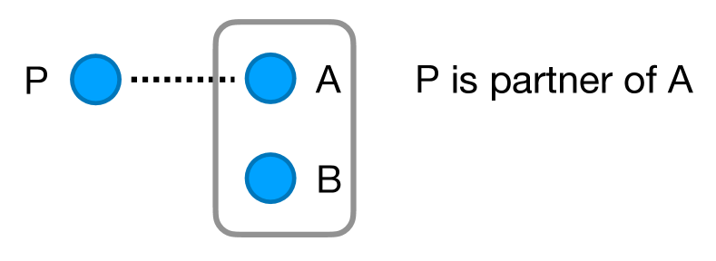
Figure 1: Setup of our problem. We introduce local modes A and B (detector modes) from the quantum field and investigate entanglement of the bipartite state AB. P denotes the partner mode of A that purifies mode A.

In this paper, we discuss the criterion for successful entanglement harvesting from the perspective of the partner formula. We show that Simon’s entanglement criterion (the entanglement criterion which appears in the Lemma of Simon’s paper [30]) for detector modes A and B can be rewritten in terms of commutators between the canonical operators of the detector mode B and the partner mode P of the detector mode A. Using the profile representation of detector modes, we demonstrate that Simon’s criterion supports our intuitive understanding of the relationship between the partner formula and the feasibility of entanglement harvesting: the overlap of the profile functions of the detector modes P and B is necessary for extracting entanglement by using detector modes A and B. Indeed, both this overlap condition and Simon’s criterion are necessary conditions for entanglement, with the overlap condition being weaker than Simon’s criterion. Therefore, detector modes A and B can be separable even if the profile functions of P and B overlap. An interesting example is entanglement harvesting by using a detector mode defined as a superposition of the Rindler modes in the right wedge of the Minkowski spacetime (region I). By examining the profile functions of the detector mode, we observe that for a single Rindler mode, its profile and the profile of the partner appear on the opposite side of the horizon [31, 22]. In contrast, when the detector mode A is defined as a linear combination of the Rindler modes, the profile of the partner mode P leaks across the horizon due to the nonlinearity of the partner relation. Intuitively, it may seem possible to extract entanglement by using two detector modes A and B consisting solely of the Rindler modes in Region I, as the profile functions of the partner mode P and that of B overlap. However, Simon’s criterion reveals that the detector modes A and B are separable when they consist only of positive frequency Rindler modes. By analogy with Hawking radiation and the Unruh effect, this result implies that no quantum correlation exists between “real particles” emitted as Hawking radiation during the early stage of black hole evaporation, since these real particles emitted as Hawking radiation correspond to the Rindler modes in this analogy.

The organization of this paper is as follows: In Sec. II, we parametrize Gaussian local modes using squeezing and rotation parameters and characterize the covariance matrix in terms of these parameters. In Sec. III, we reformulate Simon’s entanglement criterion using the partner formula. In Sec. IV, we introduce the profile representation of local modes and present the entanglement criterion in this representation. In Sec. V, we apply the criterion to the quantum field in Rindler spacetime. Sec. VI is devoted to conclusion.

II Parametrization of Modes and Entanglement

As we shall see in Sec. IV, the detector modes of the quantum field are expressed as linear combinations of the annihilation and creation operators of the quantum field, as the field operators can be expanded in terms of these operators. Hence, the detector modes of the quantum field can be analyzed within the framework of Gaussian quantum information(quantum information for harmonic oscillators). In this section, we will construct a general framework applicable to general oscillator modes before discussing the quantum field.

Let us consider two independent oscillator modes $\hat{a}_{A}$ and $\hat{a}_{B}$ embedded in $n$-mode Gaussian modes specified by the annihilation operators $\{\hat{b}_{1},\cdots,\hat{b}_{n}\}$:

$$\hat{a}_{A}:=\sum_{i=1}^{n}\left\{\alpha_{i}^{A}\hat{b}_{i}+\beta_{i}^{A}(\hat{b}_{i})^{\dagger}\right\},\quad\hat{a}_{B}:=\sum_{i=1}^{n}\left\{\alpha_{i}^{B}\hat{b}_{i}+\beta_{i}^{B}(\hat{b}_{i})^{\dagger}\right\},$$ (1)

$$\sum_{i}(|\alpha_{i}^{A}|^{2}-|\beta_{i}^{A}|^{2})=1,\quad\sum_{i}(|\alpha_{i}^{B}|^{2}-|\beta_{i}^{B}|^{2})=1.$$ (2)

By performing a basis transformation (see Appendix A for the detailed calculation), $\hat{a}_{A}$ and $\hat{a}_{B}$ can be rewritten as:

$$\hat{a}_{A} =\cosh r\,\hat{a}_{\parallel}+\sinh r\,\hat{a}^{\dagger}_{\perp},$$ (3)

$$\hat{{a}}_{B} =\cosh r_{1}\left(\cos\theta_{1}\,\hat{a}_{\parallel}+\sin\theta_{1}\cos\xi_{1}\,\hat{a}_{\perp}+\sin\theta_{1}\sin\xi_{1}\,\hat{a}_{0}\right)$$

$$+\sinh r_{1}\left(\cos\theta_{2}\,\hat{a}_{\parallel}^{\dagger}+\sin\theta_{2}\cos\xi_{2}\,\hat{a}_{\perp}^{\dagger}+\sin\theta_{2}\sin\xi_{2}\cos\chi\,\hat{a}_{0}^{\dagger}+\sin\theta_{2}\sin\xi_{2}\sin\chi\,\hat{a}_{1}^{\dagger}\right),$$ (4)

where $\hat{a}_{\parallel}$ and $\hat{a}_{\perp}$ denote independent modes that decompose the given mode A to the superposition of two modes, and $\hat{a}_{0}$ and $\hat{a}_{1}$ are bases of the oscillator modes which are orthogonal to $\hat{a}_{\parallel}$ and $\hat{a}_{\perp}$. To ensure the independence of the $\hat{a}_{A}$ and $\hat{{a}}_{B}$, we require

$$0 =[\hat{a}_{A},\hat{{a}}_{B}]=\cosh r\sinh r_{1}\cos\theta_{2}-\sinh r\cosh r_{1}\sin\theta_{1}\cos\xi_{1},$$ (5)

$$0 =[\hat{a}_{A}^{\dagger},\hat{a}_{B}]=-\cosh r\cosh r_{1}\cos\theta_{1}+\sinh r\sinh r_{1}\sin\theta_{2}\cos\xi_{2}.$$ (6)

Using these relations, we can determine the parameters $\xi_{1}$ and $\theta_{1}$ for given $r,r_{1},\theta_{2},\xi_{2}$.

In the following, we consider the vacuum state $\ket{0000}_{\parallel\perp 01}$ with $\hat{a}_{\parallel}\ket{0000}_{\parallel\perp 01}=\hat{a}_{\perp}\ket{0000}_{\parallel\perp 01}=\hat{a}_{0}\ket{0000}_{\parallel\perp 01}=\hat{a}_{1}\ket{0000}_{\parallel\perp 01}=0$ and entanglement extraction from this vacuum state with two detector modes A and B. To quantify the entanglement between these two modes, we use the covariance matrix for bipartite states, defined as

$$V^{(AB)}\equiv\left(\begin{array}[]{cc}V_{AA}&V_{AB}\\ V_{AB}^{T}&V_{BB}\end{array}\right)=\left(\begin{array}[]{cccc}\langle\{\hat{q}_{A},\hat{q}_{A}\}\rangle&\langle\{\hat{q}_{A},\hat{p}_{A}\}\rangle&\langle\{\hat{q}_{A},\hat{{q}}_{B}\}\rangle&\langle\{\hat{q}_{A},\hat{{p}}_{B}\}\rangle\\ \langle\{\hat{p}_{A},\hat{{q}}_{A}\}\rangle&\langle\{\hat{p}_{A},\hat{{p}}_{A}\}\rangle&\langle\{\hat{p}_{A},\hat{{q}}_{B}\}\rangle&\langle\{\hat{{p}}_{A},\hat{{p}}_{B}\}\rangle\\ \langle\{\hat{q}_{B},\hat{{q}}_{A}\}\rangle&\langle\{\hat{q}_{B},\hat{{p}}_{A}\}\rangle&\langle\{\hat{{q}}_{B},\hat{{q}}_{B}\}\rangle&\langle\{\hat{q}_{B},\hat{p}_{B}\}\rangle\\ \langle\{\hat{{p}}_{B},\hat{q}_{A}\}\rangle&\langle\{\hat{{p}}_{B},\hat{{p}}_{A}\}\rangle&\langle\{\hat{{p}}_{B},\hat{q}_{B}\}\rangle&\langle\{\hat{{p}}_{B},\hat{{p}}_{B}\}\rangle\end{array}\right),$$ (13)

where $\hat{q}_{A},\hat{p}_{A},\hat{q}_{B},\hat{p}_{B}$ are the canonical operators corresponding to modes A and B defined as

$$\hat{q}_{A}=\frac{\hat{a}_{A}+\hat{a}_{A}{}^{\dagger}}{\sqrt{2}},\quad\hat{p}_{A}=\frac{\hat{a}_{A}-\hat{a}_{A}{}^{\dagger}}{i\sqrt{2}},\quad\hat{q}_{B}=\frac{\hat{a}_{B}+\hat{a}_{B}{}^{\dagger}}{\sqrt{2}},\quad\hat{p}_{B}=\frac{\hat{a}_{B}-\hat{a}_{B}{}^{\dagger}}{i\sqrt{2}}.$$ (14)

For the vacuum state $|0000\rangle_{\parallel\perp 01}$, the expectation values in the covariances are evaluated as

$$\langle\{\hat{q}_{A},\hat{{q}}_{A}\}\rangle =\langle\{\hat{p}_{A},\hat{{p}}_{A}\}\rangle=\cosh 2r,$$ (15)

$$\langle\{\hat{q}_{A},\hat{{q}}_{B}\}\rangle =\cosh r(\cosh r_{1}\cos\theta_{1}+\sinh r_{1}\cos\theta_{2})+\sinh r(\cosh r_{1}\sin\theta_{1}\cos\xi_{1}+\sinh r_{1}\sin\theta_{2}\cos\xi_{2}),$$ (16)

$$\langle\{\hat{p}_{A},\hat{{p}}_{B}\}\rangle =\cosh r(\cosh r_{1}\cos\theta_{1}-\sinh r_{1}\cos\theta_{2})-\sinh r(\cosh r_{1}\sin\theta_{1}\cos\xi_{1}-\sinh r_{1}\sin\theta_{2}\cos\xi_{2}),$$ (17)

$$\langle\{\hat{{q}}_{B},\hat{{q}}_{B}\}\rangle =(\cosh r_{1}\cos\theta_{1}+\sinh r_{1}\cos\theta_{2})^{2}+(\cosh r_{1}\sin\theta_{1}\cos\xi_{1}+\sinh r_{1}\sin\theta_{2}\cos\xi_{2})^{2}$$

$$\vskip 56.9055pt+(\cosh r_{1}\sin\theta_{1}\sin\xi_{1}+\sinh r_{1}\sin\theta_{2}\sin\xi_{2}\cos\chi)^{2}+\sinh^{2}r_{1}\sin^{2}\theta_{2}\sin^{2}\xi_{2}\sin^{2}\chi,$$ (18)

$$\langle\{\hat{{p}}_{B},\hat{{p}}_{B}\}\rangle =(\cosh r_{1}\cos\theta_{1}-\sinh r_{1}\cos\theta_{2})^{2}+(\cosh r_{1}\sin\theta_{1}\cos\xi_{1}-\sinh r_{1}\sin\theta_{2}\cos\xi_{2})^{2}$$

$$\vskip 56.9055pt+(\cosh r_{1}\sin\theta_{1}\sin\xi_{1}-\sinh r_{1}\sin\theta_{2}\sin\xi_{2}\cos\chi)^{2}+\sinh^{2}r_{1}\sin^{2}\theta_{2}\sin^{2}\xi_{2}\sin^{2}\chi,$$ (19)

and all other covariances vanish. When we choose $\theta_{2}=0$, the independency conditions imply $\theta_{1}=\pi/2$ and $\xi_{1}=0$. Under such conditions, the covariance matrix adopts the conventional standard form of a bipartite Gaussian modes system:

$$V^{(AB)}_{\text{standard}}=\begin{bmatrix}a&0&c_{1}&0\\ 0&a&0&c_{2}\\ c_{1}&0&b&0\\ 0&c_{2}&0&b\end{bmatrix},$$ (20)

where $a=\cosh 2r$, $b=\cosh 2r_{1}$ and $c_{1}=-c_{2}=2\cosh r\sinh r_{1}$. This state reduces to a pure two-mode state (two-mode squeezed state) especially when $r=r_{1}$. Under this choice of the parameters, the covariance matrix reduces to the standard form with $c_{1}c_{2}<0$, however, it is also possible to reduce to the standard form with $c_{1}c_{2}\geq 0$, by different choices of parameters.

We can quantify the entanglement between two modes using the PPT criterion [32, 33, 30], which provides the necessary and sufficient condition for the entanglement of the bipartite Gaussian state. In this criterion, we evaluate symplectic eigenvalues of the partially transposed covariance matrix to test the PPT criterion; the existence of negative eigenvalues provides the necessary and sufficient condition of entanglement for bipartite Gaussian states. In some situations, it is sufficient to apply a weaker entanglement criterion, which is easier to check. Simon showed [30] that the following condition is a necessary condition for entanglement of the bipartite state AB:

$$\det V_{AB}<0.$$ (21)

By using the independence conditions Eqs. (5) and (6), we can eliminate $\theta_{1}$ and $\xi_{1}$ from $\left\langle\left\{\hat{q}_{A},\hat{q}_{B}\right\}\right\rangle$ and $\left\langle\left\{\hat{q}_{A},\hat{q}_{B}\right\}\right\rangle$, and simplify $V_{AB}$ :

$$\left\langle\left\{\hat{q}_{A},\hat{q}_{B}\right\}\right\rangle=2\left(\cosh r\cos\theta_{2}+\sinh r\sin\theta_{2}\cos\xi_{2}\right)\sinh r_{1},$$

$$\left\langle\left\{\hat{p}_{A},\hat{p}_{B}\right\}\right\rangle=-2\left(\cosh r\cos\theta_{2}-\sinh r\sin\theta_{2}\cos\xi_{2}\right)\sinh r_{1}.$$ (22)

Hence, the determinants of covariance submatrices are given as

$$\det V_{AA} =\cosh^{2}2r,$$ (23)

$$\det V_{AB} =-4\left(\cosh^{2}r\cos^{2}\theta_{2}-\sinh^{2}r\sin^{2}\theta_{2}\cos^{2}\xi_{2}\right)\sinh^{2}r_{1}.$$ (24)

III Condition for Entanglement and Its Relation with the Partner Formula

Based on the partner formula [22], the mode that purifies the mode $\hat{a}_{A}$ in Eq. (3) is given by

$$\hat{a}_{P}=\cosh r\,\hat{a}_{\perp}+\sinh r\,\hat{a}_{\parallel}^{\dagger}.$$ (25)

Actually, using the canonical variables $\hat{\xi}_{j}=(\hat{q}_{A},\hat{p}_{A},\hat{q}_{P},\hat{p}_{P})$, the covariance matrix for the bipartite state AP becomes

$$(V^{(AP)})_{jk}=\expectationvalue{\{\hat{\xi}_{j},\hat{\xi}_{k}\}}=\begin{pmatrix}\cosh 2r&0&\sinh 2r&0\\ 0&\cosh 2r&0&-\sinh 2r\\ \sinh 2r&0&\cosh 2r&0\\ 0&-\sinh 2r&0&\cosh 2r\end{pmatrix},$$ (26)

which is a pure two-mode squeezed state. In the intuitive sense, the possibility of entanglement harvesting with detector mode $\hat{a}_{A}$ and $\hat{a}_{B}$ is related to “how detector mode $\hat{a}_{B}$ and partner mode $\hat{a}_{P}$ of detector mode $\hat{a}_{A}$ resemble”. Hotta et al. used the commutation relation between the creation and annihilation operators of two modes B and P as an inner product of two modes [22], and showed the independence of these modes. Following their strategy, we consider two types of commutators between the mode $\hat{a}_{B}$ and $\hat{a}_{P}$:

$$[\hat{{a}}_{B},\hat{a}_{P}^{\dagger}] =-\sinh r\sinh r_{1}\cos\theta_{2}+\cosh r\cosh r_{1}\sin\theta_{1}\cos\xi_{1},$$ (27)

$$[\hat{a}_{B},\hat{a}_{P}] =\sinh r\cosh r_{1}\cos\theta_{1}-\cosh r\sinh r_{1}\sin\theta_{2}\cos\xi_{2}.$$ (28)

Using the independency conditions of $\hat{a}_{A}$ and $\hat{a}_{B}$, we obtain

$$[\hat{a}_{B},\hat{a}_{P}^{\dagger}] =\frac{\cos\theta_{2}}{\sinh r}\sinh r_{1},$$ (29)

$$[\hat{a}_{B},\hat{a}_{P}] =-\frac{\sin\theta_{2}\cos\xi_{2}}{\cosh r}\sinh r_{1}.$$ (30)

However, these are not invariants under the local symplectic transformations of each mode. In fact, under the following local transformation of the detector mode B

$$\hat{{a}}^{\prime}_{B}=e^{i\phi_{1}}\cosh{r}^{\prime}\,\hat{a}_{B}+e^{i\phi_{2}}\sinh{r}^{\prime}\,\hat{a}_{B}^{\dagger},$$ (31)

the quantities on the right-hand side of Eqs. (27) and (28) become completely different, although the correlation between $\hat{a}_{A}$ and $\hat{a}_{B}$ should not be changed by the local transformation.

To find quantities that are invariant under the local symplectic transformation, we focus on the covariance matrix $V=V^{(AB)}$ and its symplectic transformation under the canonical transformation of modes:

$${V}^{\prime}=SVS^{T},$$ (32)

where $S$ is the symplectic matrix satisfying

$$SJS^{T}=J,\ \ J=\left(\begin{array}[]{cc}0&1\\ -1&0\end{array}\right)\oplus\left(\begin{array}[]{cc}0&1\\ -1&0\end{array}\right).$$ (37)

The local symplectic transformation is represented by

$$S=S_{A}\oplus S_{B},$$ (38)

where ${S}_{A}$ and $S_{B}$ are the symplectic matrices for single modes A and B, respectively. Applying this transformation, the covariance matrix is transformed as

$${V}^{\prime}=\begin{pmatrix}S_{A}\,V_{AA}\,S_{A}^{T}&S_{A}\,V_{AB}\,S_{B}^{T}\\ S_{B}\,V^{T}_{AB}\,S_{A}^{T}&S_{B}\,V_{BB}\,S_{B}^{T}\end{pmatrix}.$$ (39)

From the symplectic condition $\det S=1$, we have four symplectic invariants $\det V,\det V_{AA},\det V_{AB},\det V_{BB}$, that are invariant under the local symplectic transformation.

On the other hand, we find that the quantity $-\left|[\hat{a}_{B},\hat{a}_{P}^{\dagger}]\right|^{2}+\left|\left[\hat{a}_{B},\hat{a}_{P}\right]\right|^{2}$ is invariant under the local mode transformation; Recalling equations Eqs. (23) and (24), we can directly check that this discriminant can be connected to the symplectic invariants as

$$D:=-\left|[\hat{a}_{B},\hat{a}_{P}^{\dagger}]\right|^{2}+\left|[\hat{a}_{B},\hat{a}_{P}]\right|^{2}=\frac{\det V_{AB}}{\det V_{AA}-1}.$$ (40)

Noting that $\det V_{AA}\geq 1$, Simon’s necessary condition for entanglement can be rewritten as

$$D<0.$$ (41)

Therefore, as one application of the concept of entanglement partner and the partner formula, it is possible to test whether two detector modes satisfy the necessary condition for entanglement. We can also show that the criterion using the discriminant $D$ is applicable even when the detector mode A contains single mode squeezing (see Appendix B for the proof in this case):

$$\hat{a}_{A}:=\cosh r\,\hat{a}_{\parallel}+\sinh r\cos\theta\,\hat{a}_{\parallel}^{\dagger}+\sinh r\sin\theta\,\hat{a}_{\perp}^{\dagger}.$$ (42)

Hence, we can use this criterion even if the definitions of the modes are different from Eq. (3) or Eq. (II), since any covariance matrix of the bipartite Gaussian state can be transformed to Eq. (13) by the local mode transformation.

IV Profile Function Representations of the Local Modes and the Entanglement Criterion

In the paper by Trevison et al. [23], the detector mode and its partner mode of the quantum field are represented as smeared field operators. In this section, we briefly review their method and confirm that the detector mode expressed as smeared field operators is equivalent to the detector mode represented using annihilation operators. Furthermore, we show how Simon’s criterion in the previous section can be represented in terms of profile functions that define smeared field operators.

Here, we start from a pair of the canonical operators $\{\hat{Q}_{A},\hat{P}_{A}\}$ defined through smeared field operators in $(1+1)$-dimensional spacetimes:

$$\hat{Q}_{A} :=\int dx\left\{V_{A}(x)\,\hat{\phi}(t,x)+W_{A}(x)\,\hat{\Pi}(t,x)\right\},$$ (43)

$$\hat{P}_{A} :=\int dx\left\{X_{A}(x)\,\hat{\phi}(t,x)+Y_{A}(x)\,\hat{\Pi}(t,x)\right\},$$ (44)

where $\hat{\Pi}=\partial_{t}\hat{\phi}$ is the conjugate momentum of the field operator $\hat{\phi}$, and $V_{A}(t,x)$, $W_{A}(t,x)$, $X_{A}(t,x)$, and $Y_{A}(t,x)$ are real profile functions that satisfy the condition

$$\int dx\left\{V_{A}(x)Y_{A}(x)-W_{A}(x)X_{A}(x)\right\}=1,$$ (45)

which comes from the canonical commutation relation $[\hat{Q}_{A},\hat{P}_{A}]=i$. This pair of canonical operators defines the measurements or other local operations on the quantum field; conversely, a given local operation determines the corresponding pair of canonical operators or profile functions.

As in the case of harmonic oscillators, we define the annihilation operator $\hat{a}_{A}$ as

$$\hat{a}_{A}:=\frac{\hat{Q}_{A}+i\hat{P}_{A}}{\sqrt{2}}.$$ (46)

Using the canonical commutation relation, we can confirm that the commutation relation for the creation and annihilation operators $[\hat{a}_{A},\hat{a}_{A}^{\dagger}]=1$ is satisfied. By using the mode expansion of the field operator

$$\hat{\phi}(t,x)=\int_{0}^{\infty}d\omega\,(\varphi_{\omega}(t,x)\hat{a}_{\omega}+\varphi^{*}_{\omega}(t,x)\hat{a}^{\dagger}_{\omega}),\quad[\hat{a}_{\omega_{1}},\hat{a}^{\dagger}_{\omega_{2}}]=\delta_{\omega_{1},\omega_{2}},$$ (47)

the operator $\hat{a}_{A}$ can be expressed as the linear combination of the creation operators $\hat{a}_{\omega}$:

$$\hat{a}_{A} =\frac{1}{\sqrt{2}}\int dx\,d\omega\Bigl{[}\left(V_{A}(x)+iX_{A}(x)\right)\varphi_{\omega}(t,x)+\left(W_{A}(x)+iY_{A}(x)\right)\partial_{t}\varphi_{\omega}(t,x)\Bigr{]}\hat{a}_{\omega}$$

$$\quad+\frac{1}{\sqrt{2}}\int dx\,d\omega\Bigl{[}\left(V_{A}(x)+iX_{A}(x)\right)\varphi_{\omega}^{*}(t,x)+\left(W_{A}(x)+iY_{A}(x)\right)\partial_{t}\varphi_{\omega}^{*}(t,x)\Bigr{]}\hat{a}_{\omega}^{\dagger}.$$ (48)

Therefore, the relation between the annihilation operators $\hat{a}_{A}$ and $\hat{a}_{\omega}$ is interpreted as the Bogoliubov transformation. This implies that a particle detector corresponding to $\hat{a}_{A}$ may detect particles even when the field is in the vacuum state associated with $\{\hat{a}_{\omega}\}$.

To elucidate the detailed structure of the Bogoliubov transformation, we introduce annihilation operators $\hat{a}_{\tilde{\parallel}}$ and $\hat{a}_{\perp}$ defined below and rewrite $\hat{a}_{A}$ as

$$\hat{a}_{A}=\cosh\tilde{r}\,\hat{\tilde{a}}_{\parallel}+e^{-i\phi_{1}}\sinh\tilde{r}\cos\tilde{\theta}\,\hat{\tilde{a}}_{\parallel}^{\dagger}+\sinh\tilde{r}\sin\tilde{\theta}\,\hat{a}_{\perp}^{\dagger},$$ (49)

where the annihilation operators $\hat{\tilde{a}}_{\parallel}$ and $\hat{a}_{\perp}$ are identified as

$$\hat{\tilde{a}}_{\parallel}:=\frac{1}{\sqrt{2}\cosh\tilde{r}}\int dx\,d\omega\left\{\left(V_{A}(x)+iX_{A}(x)\right)\varphi_{\omega}(t,x)+\left(W_{A}(x)+iY_{A}(x)\right)\partial_{t}\varphi_{\omega}(t,x)\right\}\hat{a}_{\omega},$$

$$\hat{a}_{\perp}:=\frac{1}{\sinh\tilde{r}\sin\tilde{\theta}}\Biggl{[}\frac{1}{\sqrt{2}}\int dx\,d\omega\left\{\left(V_{A}(x)-iX_{A}(x)\right)\varphi_{\omega}(t,x)+\left(W_{A}(x)-iY_{A}(x)\right)\partial_{t}\varphi_{\omega}(t,x)\right\}\hat{a}_{\omega}$$

$$\qquad\qquad\qquad\qquad\qquad\qquad\qquad\qquad\qquad\qquad\qquad\qquad\qquad\qquad\qquad\qquad-e^{i\phi_{1}}\sinh\tilde{r}\cos\tilde{\theta}\,\hat{\tilde{a}}_{\parallel}\Biggr{]}.$$ (50)

The coefficients in (49) are fixed by commutation relations between $\hat{\tilde{a}}_{\parallel}$ and $\hat{a}_{\perp}$:

$$\cosh^{2}\tilde{r}=\frac{1}{2}\int d\omega\left|\int dx\left\{\left(V_{A}(x)+iX_{A}(x)\right)\varphi_{\omega}(t,x)+\left(W_{A}(x)+iY_{A}(x)\right)\partial_{t}\varphi_{\omega}(t,x)\right\}\right|^{2},$$

$$\cos\tilde{\theta}=\frac{1}{\sinh\tilde{r}}\left|\left[\hat{\tilde{a}}_{\parallel},\frac{1}{\sqrt{2}}\int dxd\omega\left\{\left(V_{A}(x)+iX_{A}(x)\right)\varphi^{*}_{\omega}(t,x)+\left(W_{A}(x)+iY_{A}(x)\right)\partial_{t}\varphi^{*}_{\omega}(t,x)\right\}\hat{a}_{\omega}^{\dagger}\right]\right|,$$

$$\phi_{1}=\arg\left\{\left[\hat{\tilde{a}}_{\parallel},\frac{1}{\sqrt{2}}\int dxd\omega\left\{\left(V_{A}(x)+iX_{A}(x)\right)\varphi_{\omega}^{*}(t,x)+\left(W_{A}(x)+iY_{A}(x)\right)\partial_{t}\varphi_{\omega}^{*}(t,x)\right\}\hat{a}_{\omega}^{\dagger}\right]\right\}.$$ (51)

By performing the following local symplectic transformation

$$\hat{a}_{\parallel}=e^{i\tilde{\phi}_{1}}\cosh{r^{\prime}}\,\hat{\tilde{a}}_{\parallel}+e^{-i\tilde{\phi}_{2}}\sinh r^{\prime}\,\hat{\tilde{a}}_{\parallel}^{\dagger},$$ (52)

with appropriate parameters $r^{\prime}$, $\tilde{\phi}_{1}$, $\tilde{\phi}_{2}$ which characterize the local mode transformation, the annihilation operator $\hat{a}_{A}$ reduces to the oscillator mode defined in Eq. (3). Therefore, it is possible to obtain the annihilation operator representation from the profile function representation. Conversely, if the relationship between a pair of operators $\{\hat{a}_{\parallel},\hat{a}_{\perp}\}$ and $\{\hat{a}_{\omega}\}$ is specified, the profile functions of the local mode can be reconstructed by following the procedure described above in reverse. Thus, the representation in terms of creation and annihilation operators (Eq. (3)) and the profile function representation (Eqs. (43) and (44)) of the detector mode are equivalent.

Now, let us consider entanglement harvesting from the quantum field using two detector modes A and B. The situation is described as follows: the detector mode B is initially configured with the use of profile functions, as

$$\hat{Q}_{B} :=\int dx\left\{V_{B}(x)\,\hat{\phi}(t,x)+W_{B}(x)\,\hat{\Pi}(t,x)\right\},$$ (53)

$$\hat{P}_{B} :=\int dx\left\{X_{B}(x)\,\hat{\phi}(t,x)+Y_{B}(x)\,\hat{\Pi}(t,x)\right\}.$$ (54)

The detector mode A is specified indirectly through its partner mode instead of specifying it directly:

$$\hat{Q}_{P} :=\int dx\left\{V_{P}(x)\,\hat{\phi}(t,x)+W_{P}(x)\,\hat{\Pi}(t,x)\right\},$$ (55)

$$\hat{P}_{P} :=\int dx\left\{X_{P}(x)\,\hat{\phi}(t,x)+Y_{P}(x)\,\hat{\Pi}(t,x)\right\}.$$ (56)

To apply Simon’s necessary condition Eq. (21) for the bipartite entanglement, we evaluate $D$ defined in Eq. (40):

$$D: =-\left|\left[\hat{a}_{P},\hat{a}_{B}^{\dagger}\right]\right|^{2}+\left|\left[\hat{a}_{P},\hat{a}_{B}\right]\right|^{2}$$

$$=2\left(-[\hat{Q}_{P},\hat{Q}_{B}][\hat{P}_{P},\hat{P}_{B}]^{*}+[\hat{P}_{P},\hat{Q}_{B}][\hat{Q}_{P},\hat{P}_{B}]^{*}\right),$$ (57)

where we used the fact that the commutator of canonical operators is purely imaginary to derive the last line. Expressing the commutators in terms of the profile functions, we have:

$$[\hat{Q}_{P},\hat{Q}_{B}]=i\int dx\,(V_{P}W_{B}-W_{P}V_{B}),\quad[\hat{P}_{P},\hat{P}_{B}]=i\int dx\,(X_{P}Y_{B}-Y_{P}X_{B}),$$ (58)

$$[\hat{P}_{P},\hat{Q}_{B}]=i\int dx\,(X_{P}W_{B}-Y_{P}V_{B}),\quad[\hat{Q}_{P},\hat{P}_{B}]=i\int dx\,(V_{P}Y_{B}-W_{P}X_{B}).$$ (59)

We observe that these commutators vanish when the pairs of the profile functions $\{V_{B},W_{B},X_{B},Y_{B}\}$ and
$\{V_{P},W_{P},X_{P},Y_{P}\}$ have no overlap. In this case, $D=0$ and harvesting entanglement from a quantum field cannot be achieved through the detector modes A and B. Hence, an overlap between the profile functions of mode B and the profile functions of partner mode P of A, which correlates with the detector mode A, is necessary for extracting entanglement using the detector modes A and B. Consideration in this section reinforces our intuitive understanding of the profile function representation of the local modes: the support of the detector mode’s profile functions corresponds to the location of the detector mode, while the support of the partner mode’s profile functions corresponds to the location of the partner.

V Example in the Unruh Effect

In the previous subsection, we observed that the overlap between detector mode B and the partner P of another detector mode A provides one criterion for entanglement harvesting, since the overlap of these profiles is necessary for the entanglement. However, overlap of the profile functions generally does not provide a sufficient condition. We can see this in the example of the superposed Rindler modes. In this section, we only consider the left-moving mode of a chiral quantum field.

V.1 Rindler mode, Its Partner and Unruh Effect

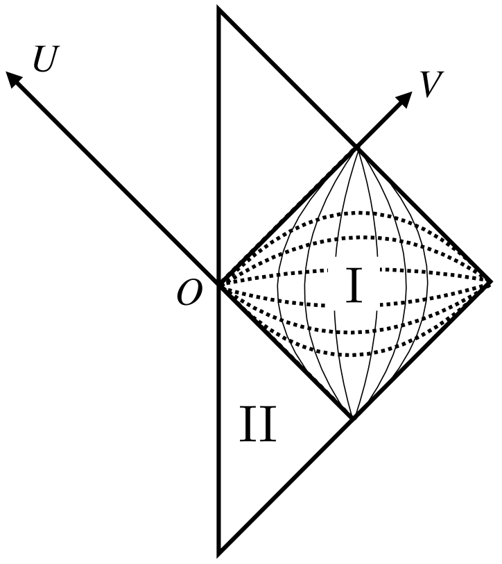
Figure 2: Penrose diagram depicting one-half of the Minkowski spacetime. In region I, the solid lines denote surfaces of constant $\xi$, while the dashed lines indicate surfaces of constant $\eta$.

In this subsection, we briefly review the Unruh effect [3, 4, 29]. We consider a massless scalar field in the $(1+1)$-dimensional Minkowski spacetime, satisfying the Klein-Gordon equation $\square\phi=0$. We begin with an examination of the structure of Minkowski spacetime before proceeding to analyze the scalar field. The metric is

$$ds^{2}=-dt^{2}+dx^{2}.$$ (60)

For later use, we introduce null coordinates $U=t-x,\ V=t+x$. The metric can be expressed as $ds^{2}=-dUdV$. Now, let us consider new coordinates $(\eta,\xi)$ which are related to Minkowski coordinates $(t,x)$ by

$$t =\frac{1}{a}e^{a\xi}\sinh a\eta,\quad x=\frac{1}{a}e^{a\xi}\cosh a\eta,\quad-\infty<\eta<+\infty,\quad-\infty<\xi<+\infty.$$ (61)

This new coordinate system is called the Rindler coordinates, which is the coordinate system accompanied by a uniformly accelerating observer. The metric with the Rindler coordinates is given by

$$ds^{2}=-e^{2a\xi}(d\eta^{2}-d\xi^{2}).$$ (62)

The important property of the Rindler coordinates is that these coordinates cover only region I of the Minkowski spacetime (see Fig. 2). Thus, the accelerating observer can only see a part of the spacetime. We introduce null coordinates for the Rindler coordinates $u=\eta-\xi,~v=\eta+\xi$. The metric with the null coordinates is expressed as

$$ds^{2}=-e^{2a\xi}\,du\,dv.$$ (63)

The null coordinates of the Minkowski spacetime and the Rindler coordinates are related as

$$U =-\frac{1}{a}\,e^{-au},\quad V=\frac{1}{a}\,e^{av}.$$ (64)

Using the null coordinates, the field equation can be written as $\partial_{U}\partial_{V}\phi(U,V)=0$ in the Minkowski coordinates and $\partial_{u}\partial_{v}\phi(u,v)=0$ in the Rindler coordinates. In the Rindler coordinates, the left-moving mode function in region I is defined by

$$\phi^{\text{I}}_{\omega}(V): =\frac{1}{\sqrt{4\pi|\omega|}}\exp(-i\omega v(V))\,\theta(V)$$

$$=\frac{1}{\sqrt{4\pi|\omega|}}\exp\left(-i\frac{\omega}{a}\log(aV)\right)\theta(V),\quad\omega>0,$$ (65)

where we multiplied the step function $\theta(V)$ to ensure that the Rindler coordinates cover only region I and the mode function $\phi_{\omega}^{\text{I}}$ has support only in region I. It is also possible to introduce a mode function in region II defined by

$$\phi^{\text{II}}_{\omega}(V): =\frac{1}{\sqrt{4\pi|\omega|}}\exp(-i\omega v(-V))\theta(-V)$$

$$=\frac{1}{\sqrt{4\pi|\omega|}}\exp\left(-i\frac{\omega}{a}\log(-aV)\right)\theta(-V),\quad\omega>0.$$ (66)

We notice that $\phi^{\text{II}}_{\omega}(V)$ has a negative norm and to obtain the positive norm modes, we need to take the complex conjugate for this mode. In fact, the positive norm mode $\phi^{\text{II}}_{-\omega}(V)=(\phi^{\text{II}}_{\omega}{}(V)){}^{*}$ is known as the Milne mode.

Although the mode functions $\phi^{\text{I}}_{\omega}$ and $\phi^{\text{II}}_{\omega}$ are non-analytic, the following functions defined by linear combinations of $\phi^{\text{I}}_{\omega}$ and $\phi^{\text{II}}_{\omega}$ are analytic in the whole Minkowski spacetime:

$$\Phi_{\omega}(V) :=\frac{e^{\pi\omega/2a}\,\phi^{\text{I}}_{\omega}(V)+e^{-\pi\omega/2a}\,(\phi^{\text{II}}_{-\omega}(V))^{*}}{\sqrt{2\sinh(\pi\omega/a)}},$$ (67)

$$\Psi_{-\omega}(V) :=\frac{e^{-\pi\omega/2a}\,\left(\phi^{\text{I}}_{\omega}(V)\right)^{*}+e^{\pi\omega/2a}\,\phi^{\text{II}}_{-\omega}(V)}{\sqrt{2\sinh(\pi\omega/a)}}.$$ (68)

These functions are bounded everywhere in the lower-half complex $V$ plane, and orthogonal to each other. The modes defined by these functions are called Unruh modes. The analytic property of the Unruh modes implies that these modes correspond to the positive norm Minkowski modes with respect to the Klein-Gordon inner product. By solving these relations for $\phi^{\text{I}}_{\omega}$ and $\phi^{\text{II}}_{\omega}$, we obtain

$$\phi^{\text{I}}_{\omega}(V) =\alpha_{\omega}\Phi_{\omega}(V)-\beta_{\omega}\left(\Psi_{-\omega}(V)\right)^{*},$$ (69)

$$\phi^{\text{II}}_{-\omega}(V) =-\beta_{\omega}\left(\Phi_{\omega}(V)\right)^{*}+\alpha_{\omega}\,\Psi_{-\omega}(V),$$ (70)

and the coefficients are given by

$$\alpha_{\omega} :=\frac{e^{\pi\omega/2a}}{\sqrt{2\sinh(\pi\omega/a)}},\quad\beta_{\omega}:=\frac{e^{-\pi\omega/2a}}{\sqrt{2\sinh(\pi\omega/a)}},\quad\alpha_{\omega}^{2}-\beta_{\omega}^{2}=1.$$ (71)

We introduce annihilation operators by using the Klein-Gordon inner product between the field operator $\hat{\phi}$ and positive norm mode functions:

$$\hat{a}^{\text{I}}_{\omega} =(\hat{\phi},\phi^{\text{I}}_{\omega}),\hskip 14.22636pt\hat{a}^{\text{II}}_{\omega}=(\hat{\phi},\phi^{\text{II}}_{-\omega}),$$ (72)

$$\hat{a}^{\Phi}_{\omega} =(\hat{\phi},\Phi_{\omega}),\hskip 14.22636pt\hat{a}^{\Psi}_{\omega}=(\hat{\phi},\Psi_{-\omega}).$$ (73)

Using the relations for the mode functions, the corresponding annihilation operators are related as

$$\hat{a}^{\text{I}}_{\omega} =\alpha_{\omega}\,\hat{a}^{\Phi}_{\omega}+\beta_{\omega}\left(\hat{a}^{\Psi}_{\omega}\right)^{\dagger},$$ (74)

$$\hat{a}^{\text{II}}_{\omega} =\beta_{\omega}\left(\hat{a}_{\omega}^{\Phi}\right)^{\dagger}+\alpha_{\omega}\,\hat{a}^{\Psi}_{\omega}.$$ (75)

If we take $r$ such that $\sinh r=\beta_{\omega}$, the first formula Eq. (74) coincides with Eq. (3) and the second formula Eq. (75) coincides with its partner formula Eq. (25). Therefore, the Milne mode $\hat{a}_{\omega}^{\text{II}}$ is the partner mode of the Rindler mode $\hat{a}_{\omega}^{\text{I}}$.

Now, let us consider the UDW detector with two internal energy levels, moving with a constant acceleration in the Minkowski spacetime. The interaction between the detector and the scalar field in the interaction picture is assumed to be

$$\hat{H}_{int}^{\text{I}}(\tau)={\lambda}\,(e^{i\Omega\tau}\,\hat{\sigma}_{+}+e^{-i\Omega\tau}\,\hat{\sigma}_{-})\,\hat{\phi}(\tau,\xi_{0}),$$ (76)

where $\lambda$ is a coupling constant between the scalar field and the detector, $\Omega$ is the energy gap of the detector, $\hat{\sigma}_{+}$ and $\hat{\sigma}_{-}$ are ladder operators, and $\xi_{0}=\text{const.}$ is the trajectory (world line) of the detector in the comoving coordinate system of the detector. The time evolution operator is given by

$$\hat{U}=T\exp\left(-i\int d{\tau^{\prime}}\hat{H}^{\text{I}}_{int}(\tau^{\prime})\right)\simeq 1-i{\lambda}\int d{\tau^{\prime}}(e^{i\Omega\tau^{\prime}}\hat{\sigma}_{+}+e^{-i\Omega\tau^{\prime}}\hat{\sigma}_{-})\,\hat{\phi}(\tau^{\prime},\xi_{0})+O({\lambda}^{2}).$$ (77)

Adopting the mode expansion of the field operator with Rindler modes, we obtain

$$\hat{U}\simeq 1-i{\lambda}\frac{e^{i\Omega\xi_{0}}}{\sqrt{4\pi\Omega}}\,\hat{\sigma}_{+}\,\hat{a}^{\text{I}}_{\Omega}-i{\lambda}\frac{e^{-i\Omega\xi_{0}}}{\sqrt{4\pi\Omega}}\,\hat{\sigma}_{-}\left(\hat{a}^{\text{I}}_{\Omega}\right)^{\dagger}.$$ (78)

Since the mode functions $\Phi_{\omega}$ and $\Psi_{-\omega}$ only contain the positive frequency Minkowski modes, the vacuum state defined by $\hat{a}^{\Phi}_{\omega}$, $\hat{a}^{\Psi}_{\omega}$ and the Minkowski vacuum $|0\rangle_{M}$ are the same vacuum state. Therefore, if we prepare the initial state of the quantum field as the Minkowski vacuum state and the initial state of the detector state as the ground state (i.e. state satisfying $\hat{\sigma}_{-}|0\rangle_{D}=0$), the excitation probability of the detector is

$$\mathrm{Prob}\left(|0\rangle_{D}\to|1\rangle_{D}\right)\propto\frac{1}{\Omega}\,|\beta_{\Omega}|^{2}=\dfrac{1}{\Omega}\dfrac{1}{e^{2\pi\Omega/a}-1}.$$ (79)

The factor $1/(e^{2\pi\Omega/a}-1)$ represents the Planckian distribution with a temperature $T=a/2\pi$. The same thermal factor appears if we consider the transition probability of the detector immersed in the thermal bath with the temperature $T$. Therefore, we cannot distinguish the quantum field seen by the accelerating observer and the thermal quantum field by using detectors at rest. This is called the Unruh effect.

V.2 The Superposition of Rindler Modes and Its Overlapped Partner

In this subsection, we consider the detector whose mode is given by superposition of the Rindler modes:

$$\hat{a}_{A}:=\int_{0}^{\infty}d{\omega}f(\omega)\,\hat{a}^{\text{I}}_{\omega},\quad\int_{0}^{\infty}d{\omega}\,|f(\omega)|^{2}=1.$$ (80)

Using (74), this detector mode is rewritten in the form of

$$\hat{a}_{A}=\alpha\,\hat{a}_{\parallel}+\beta\,\hat{a}_{\perp}^{\dagger},$$ (81)

where we defined

$$\alpha :=\sqrt{\int_{0}^{\infty}d\omega\,|f(\omega)|^{2}\,\alpha_{\omega}^{2}},\quad\beta:=\sqrt{\int_{0}^{\infty}d\omega\,|f(\omega)|^{2}\,\beta_{\omega}^{2}},\quad\alpha^{2}-\beta^{2}=1,$$ (82)

$$\hat{a}_{\parallel} :=\frac{1}{\alpha}\int_{0}^{\infty}d\omega{f(\omega)}\alpha_{\omega}\,\hat{a}^{\Phi}_{\omega},\quad\hat{a}_{\perp}:=\frac{1}{\beta}\int_{0}^{\infty}d\omega f^{*}(\omega)\beta_{\omega}\,\hat{a}^{\Psi}_{\omega}.$$ (83)

From the partner formula (25), the partner mode P for mode A is

$$\hat{a}_{P}=\alpha\,\hat{a}_{\perp}+\beta\,\hat{a}_{\parallel}^{\dagger}.$$ (84)

This partner mode can be reformulated utilizing Rindler modes and Milne modes:

$$\hat{a}_{P}=\int_{0}^{\infty}d{\omega}\,\frac{\alpha_{\omega}\beta_{\omega}}{\alpha\beta}f^{*}(\omega)\,\hat{a}^{\text{II}}_{\omega}+\int_{0}^{\infty}d{\omega}\,\frac{\beta^{2}-\beta_{\omega}^{2}}{\alpha\beta}f^{*}(\omega)\left(\hat{a}^{\text{I}}_{\omega}\right)^{\dagger}.$$ (85)

This is a key equation in this section. The partner mode of the superposed Rindler modes is a superposition of the Milne modes and the Rindler modes with squeezing. For the single mode case, the weighting function is $|f(\omega)|^{2}=\delta(\omega-\omega_{0})$, and $\beta=\beta_{\omega_{0}}$ holds. Thus the contribution of the Rindler modes in Eq. (85) vanishes and the spatial profile of the partner mode is a mirror-reflection of the mode A’s profile with respect to the Rindler horizon $V=0$. On the other hand, in general, the superposition of modes results in the second term in Eq. (85) is not equal to zero. Typically, the partner of the Rindler modes is not restricted to region II and extends beyond the Rindler horizon. This leakage can be explicitly observed by analyzing the profile function of these modes.

The general form of detector modes in the Minkowski spacetime is given as follows:

$$\hat{a}:=\int_{0}^{\infty}d\omega\left\{A(\omega)\,\hat{a}^{\text{I}}_{\omega}+B(\omega)\left(\hat{a}^{\text{I}}_{\omega}\right)^{\dagger}+C(\omega)\,\hat{a}^{\text{II}}_{\omega}+D(\omega)\left(\hat{a}^{\text{II}}_{\omega}\right)^{\dagger}\right\},$$ (86)

where $A(\omega)$, $B({\omega})$, $C(\omega)$ and $D(\omega)$ are weighting functions. On the other hand, for a massless (chiral) scalar field, it is also possible to define the detector mode by smearing the field operator $\hat{\Pi}(V)=\partial_{V}\hat{\phi}(V)$ [20, 28, 29]:

$$\hat{Q} :=\int d{V}q(V)\,\hat{\Pi}(V),\quad\hat{P}:=\int d{V}p(V)\,\hat{\Pi}(V),$$ (87)

where the profile functions $q(V)$ and $p(V)$ of the mode are real functions chosen to satisfy the canonical commutation relation

$$[\hat{Q},\hat{P}]=-\frac{i}{2}\int d{V}q(V)\,p^{\prime}(V)\equiv i.$$ (88)

By expanding the field operator in terms of annihilation operators and comparing it with Eq. (86), we obtain the profile functions of the detector modes expressed in terms of these weighting functions (See Appendix C for detailed derivations):

$$q(V) =-2\sqrt{2}\,\operatorname{Im}\left[\int_{0}^{\infty}d\omega\left\{\left(A(\omega)+B^{*}(\omega)\right)\left(\phi_{\omega}^{\text{I}}(V)\right)^{*}+\left(C(\omega)+D^{*}(\omega)\right)\left(\phi_{-\omega}^{\text{II}}(V)\right)^{*}\right\}\right],$$ (89)

$$p(V) =2\sqrt{2}\,\operatorname{Re}\left[\int_{0}^{\infty}d\omega\left\{\left(A(\omega)-B^{*}(\omega)\right)\left(\phi_{\omega}^{\text{I}}(V)\right)^{*}+\left(C(\omega)-D^{*}(\omega)\right)\left(\phi_{-\omega}^{\text{II}}(V)\right)^{*}\right\}\right].$$ (90)

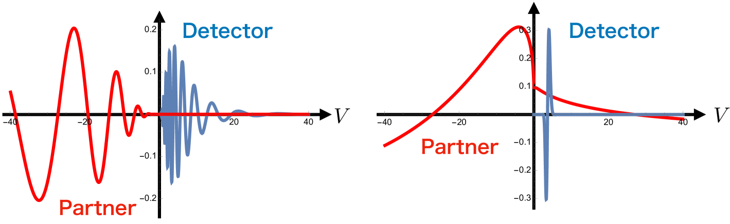
Figure 3: The profile function $q_{A}(V)$ of the detector mode A placed in region I ($V>0$). Mode A is defined by $\hat{a}_{A}:=\int_{0}^{\infty}d\omega\,\omega^{3/2}e^{-\alpha(\omega-\omega_{0})^{2}}\hat{a}^{\text{I}}_{\omega}$ (blue lines), and its partner mode $q_{P}(V)$ (red lines). The left panel shows the profile functions with $\alpha=50$, $\omega_{0}=1.5$. The right panel shows the profile functions with $\alpha=1$, $\omega_{0}=0.05$. In these plots, we choose $a=0.1$ as the acceleration of the Rindler observer.

Profiles of detector mode A and its partner mode are shown in Fig. 3. In the left panel, the weighting function $f(\omega)$ of the Rindler mode is sharply localized in the frequency domain. As a result, the detector mode A behaves as a mode with a single frequency (single mode), and its partner mode is located at the opposite side of the Rindler horizon $V=0$. However, due to the factor $\alpha_{\omega}\beta_{\omega}$ in Eq. (85) that contributes as a shift of the weighting function toward smaller frequencies, the partner wave packet is not the mirror-flipped image of the detector mode A but becomes the redshifted one. We need to consider a more sharply localized weighting function in the frequency domain ($\alpha\gg 1/a$) to reduce this redshift, but the wave packet is not localized in the configuration space in such a case. It is worth noting that the detector mode coincides with the Rindler mode in this limit. The right panel of Fig. 3 shows the profile functions for the case that the single-mode approximation is not applicable. We observe that the profile of the partner mode leaks out from the Rindler horizon in this case.

Now let us prepare another detector mode B, which consists of the superposition of Rindler modes orthogonal to mode A:

$$\hat{a}_{B}:=\int_{0}^{\infty}d{\omega}\,g(\omega)\,\hat{a}^{\text{I}}_{\omega}.$$ (91)

The weighting function $g(\omega)$ satisfies the following normalization condition and the orthogonality condition for the weighting function $f(\omega)$:

$$\int_{0}^{\infty}d\omega|g(\omega)|^{2}=1,\quad\int_{0}^{\infty}d\omega f(\omega)g^{*}(\omega)=0.$$ (92)

If we choose the weighting function $g(\omega)$ properly (for example, we take $g(\omega)\propto(\beta^{2}-\beta_{\omega}^{2})f(\omega)$ which comes from the second term of Eq. (85)), the profile function of $\hat{a}_{B}$ and the profile function of the partner mode $\hat{a}_{P}$ of $\hat{a}_{A}$ overlap, and we expect the success of entanglement harvesting from the quantum field using the bipartite detector mode AB. However, it can be shown that the harvesting with the mode AB fails by investigating the discriminant $D$ directly: From Eq. (85), the partner mode $\hat{a}_{P}$ of the superposed Rindler mode does not contain the annihilation part $\hat{a}^{\text{I}}_{\omega}$ of the Rindler mode. As a result, the following relation holds for $\hat{a}_{B}$ defined as Eq. (91),

$$[\hat{a}_{P}^{\dagger},\hat{a}_{B}]=0,$$ (93)

and the discriminant $D$ becomes greater than zero. Therefore, by Simon’s criterion, the detector modes A and B do not entangle, and the entanglement harvesting using the two detector modes A and B does not succeed.

We summarize the result of this section as the following theorem:

Theorem 1 (No-go theorem of harvesting).

It is impossible to extract entanglement from a chiral quantum field using detector modes A and B when their annihilation operators $\hat{a}_{A}$ and $\hat{a}_{B}$ consist solely of Rindler annihilation operators:

$$\hat{a}_{A}=\int_{0}^{\infty}d{\omega}f(\omega)\,\hat{a}^{\mathrm{I}}_{\omega},\quad\hat{a}_{B}=\int_{0}^{\infty}d{\omega}\,g(\omega)\,\hat{a}^{\mathrm{I}}_{\omega}.$$ (94)

This no-go theorem also holds for the Milne modes, which can be verified by replacing the Rindler modes with the Milne modes.

V.3 The case no-go theorem is not applicable

In this subsection, we explore a case where our no-go theorem is not applicable and analyze the resulting physical implications. The no-go theorem loses its applicability when the detector mode $\hat{a}_{B^{\prime}}$ is utilized, incorporating the creation component

$$\hat{a}_{B^{\prime}}=\int_{0}^{\infty}d\omega\left\{g(\omega)\,\hat{a}^{\text{I}}_{\omega}+h(\omega)\left(\hat{a}^{\text{I}}_{\omega}\right)^{\dagger}\right\},$$ (95)

as the commutator $\left[\hat{a}_{P}^{\dagger},\hat{a}_{B^{\prime}}\right]$ does not vanish. Therefore, employing the detector mode $\hat{a}_{A}$, which includes only the annihilation operator $\hat{a}_{\omega}^{\text{I}}$, alongside $\hat{a}_{B^{\prime}}$ as specified by (95), allows for entanglement extraction without restriction.

To observe the difference between $\hat{a}_{B}$ and $\hat{a}_{B^{\prime}}$, we consider two UDW detectors whose time evolution operators are given by

$$\hat{U}_{B} =1-i\lambda\left(\hat{\sigma}_{+}\,\hat{a}_{B}+\hat{\sigma}_{-}\,\hat{a}_{B}^{\dagger}\right),$$ (96)

$$\hat{U}_{B^{\prime}} =1-i\lambda\left(\hat{\sigma}_{+}\,\hat{a}_{B^{\prime}}+\hat{\sigma}_{-}\,\hat{a}_{B^{\prime}}^{\dagger}\right).$$ (97)

Now, we apply these time evolution operators to the quantum state $\left|0\right\rangle_{D}\otimes\left|0\right\rangle_{\text{I}}$ where $|0\rangle_{D}$ is the lowest energy state of the detector (i.e., $\hat{\sigma}_{-}|0\rangle_{D}=0$) and $|0\rangle_{\text{I}}$ is the Rindler vacuum state:

$$\hat{U}_{B}\left|0\right\rangle_{D}\otimes\left|0\right\rangle_{\text{I}}=|0\rangle_{D}\otimes\left|0\right\rangle_{\text{I}},$$ (98)

$$\hat{U}_{B^{\prime}}|0\rangle_{D}\otimes|0\rangle_{\text{I}}=|0\rangle_{D}\otimes|0\rangle_{\text{I}}-i\lambda\int_{0}^{\infty}d{\omega}\,h(\omega)|1\rangle_{D}\otimes|1_{\omega}\rangle_{\text{I}}.$$ (99)

On the other hand, when these time evolution operators act on the quantum state with 1-Rindler particle $|0\rangle_{D}\otimes|1_{\Omega}\rangle_{\text{I}}$, the time-evolved states are

$$\hat{U}_{B}\left|0\right\rangle_{D}\otimes\left|1_{\Omega}\right\rangle_{\text{I}}=|0\rangle_{D}\otimes|1_{\Omega}\rangle_{\text{I}}-i\lambda\,g(\Omega)|1\rangle_{D}\otimes\left|0\right\rangle_{\text{I}},$$ (100)

$$\hat{U}_{B^{\prime}}|0\rangle_{D}\otimes|1_{\Omega}\rangle_{\text{I}}=|0\rangle_{D}\otimes|1_{\Omega}\rangle_{\text{I}}-i\lambda\,g(\Omega)|1\rangle_{D}\otimes\left|0\right\rangle_{\text{I}}-i\lambda\int_{0}^{\infty}d\omega\,h(\omega)|1\rangle_{D}\otimes|1_{\omega}1_{\Omega}\rangle_{\text{I}}.$$ (101)

The time evolution by $\hat{U}_{B}$ does not excite the detector with the absence of Rindler particles, whereas it does excite the detector with some probability if Rindler particles are present. In contrast, the time evolution operator $\hat{U}_{B^{\prime}}$ can excite the detector with non-zero probability even if no Rindler particles are present.

Hence, we can say that the UDW detector with time evolution $\hat{U}_{B}$ observes the “real” Rindler particles through its excitation. Then, what does the detector corresponding to $\hat{a}_{B^{\prime}}$ observe? To investigate this, we introduce the total particle number $\hat{N}$, defined as

$$\hat{N}=\hat{N}_{D}+\int_{0}^{\infty}d{\omega}\hat{N}_{\omega}^{\text{I}},$$ (102)

where $\hat{N}_{D}:=\hat{\sigma}_{+}\hat{\sigma}_{-}$ is the number operator for the detector, and $\left\{\hat{N}_{\omega}^{\text{I}}\right\}$ are the number operators for the Rindler modes. We observe that the expectation value of $\hat{N}$ does not change under the time evolution $\hat{U}_{B}$, while it increases under the time evolution $\hat{U}_{B^{\prime}}$. Thus, the interaction including $\hat{a}_{B^{\prime}}$ performs a measurement that is accompanied by the field excitation, and its measurement outcomes contain information about “virtual” Rindler particles.

According to the considerations on Unruh’s shell collapsing model [5, 4] and the moving mirror model [31, 22, 34, 29], the Milne modes $\hat{a}_{\omega}^{\text{II}}$ are transformed into the Minkowski modes $\hat{a}_{\omega}^{\text{BH}}$ owing to the structure of spacetimes, which gives rise to Hawking radiation as the emission of real particles. Therefore, the measurement of the Minkowski modes in black hole spacetimes is equivalent to the measurement of the Milne modes in the Minkowski spacetime. Considering the relation between the Rindler modes and the Milne modes, the operators $\hat{a}_{A}$, $\hat{a}_{B}$, $\hat{a}_{B^{\prime}}$ in Eqs. (94) and (95) have the following correspondences:

$$\hat{a}_{A}\to\int_{0}^{\infty}d{\omega}f(\omega)\,\hat{a}^{\mathrm{\text{BH}}}_{\omega},\quad\hat{a}_{B}\to\int_{0}^{\infty}d{\omega}\,g(\omega)\,\hat{a}^{\mathrm{\text{BH}}}_{\omega},\quad\hat{a}_{B^{\prime}}\to\int_{0}^{\infty}d\omega\left\{g(\omega)\hat{a}^{\text{BH}}_{\omega}+h(\omega)\left(\hat{a}^{\text{BH}}_{\omega}\right)^{\dagger}\right\}.$$ (103)

Under these correspondences, $\hat{a}_{A,B}$ represents the measurement of the real particles (Hawking radiation) by the observer at the future null infinity, whereas $\hat{a}_{B^{\prime}}$ corresponds to the measurements that include contributions from “virtual particles”, or in other words, vacuum fluctuations. For the vacuum fluctuation scenario [35, 31, 22] of the black hole evaporation, our no-go theorem is applicable, and the following corollary holds:

Corollary 1 (No-go theorem for vacuum fluctuation scenario).

Extracting quantum correlations from Hawking radiation that reaches future null infinity is not feasible when considering solely real Hawking particles originating from Milne particles.

We can also apply our no-go theorem for Page’s scenario [36] of the black hole evaporation, in which the partner of the early stage Hawking radiation is identified with the late-time Hawking radiation. It is important to note that the correspondence between the Milne modes $\hat{a}^{\text{II}}_{\omega}$ and the Minkowski modes $\hat{a}^{\text{BH}}_{\omega}$ holds only during the early stage of the black hole evaporation in this case, as the late-time radiation corresponds to the Rindler modes $\hat{a}^{\text{I}}_{\omega}$. Thus, above corollary also applies to Page’s scenario, restricted to the early stage radiation. It is important to emphasize again that this no-go theorem does not forbid entanglement extraction by using vacuum fluctuations of the quantum field in black hole spacetimes.

V.4 Demonstrations

In this subsection, we numerically evaluate entanglement between two detector modes consisting of the Milne modes in region $V<0$, as a demonstration of our no-go theorem. For comparison, we consider two different types of detector modes: a detector mode with $\omega$-top-hat profile functions (type 1) and a detector mode with sin-cos profile functions (type 2). The key difference between them lies in the structure of the local operators represented with annihilation operators: the former does not include creation operators of the Milne modes, whereas the latter does. As a result, our no-go theorem does not apply to the latter detector.

The $\omega$-top-hat function detector modes $\left\{\hat{q}_{A}^{(1)},\hat{p}_{A}^{(1)},\hat{q}_{B}^{(1)},\hat{p}_{B}^{(1)}\right\}$ are defined using annihilation operators of the Milne modes as

$$\hat{a}_{A,B}^{(1)}=\int_{0}^{\infty}d{\omega}F_{A,B}^{(1)}(\omega)\,\hat{a}_{\omega}^{\text{II}},\quad\int_{0}^{\infty}d{\omega}\,|F_{A,B}^{(1)}(\omega)|^{2}=1,$$ (104)

where $F_{A,B}^{(1)}$ is the weighting function given as

$$F_{A,B}^{(1)}(\omega)=\begin{cases}\dfrac{e^{i\omega f(V_{A,B})}}{\sqrt{\omega_{+}-\omega_{-}}}&\quad\text{for}\quad\omega_{-}\leq\omega\leq\omega_{+}\\ 0&\quad\text{else}\end{cases}$$ (105)

with $0\leq\omega_{-}<\omega_{+}$. Here, the function $f(V)$ is defined as $f(V)=-(1/a)\log(-aV)$. The two detector modes become independent and satisfy the canonical commutation relations $[\hat{q}_{j}^{(1)},\hat{p}_{k}^{(1)}]=i\delta_{jk},~j,k=A,B$ if $V_{A}$ and $V_{B}$ satisfy

$$\frac{V_{B}}{V_{A}}=\exp\left[\frac{2\pi na}{\omega_{+}-\omega_{-}}\right],\ \ n=\pm 1,\pm 2,\dots.$$ (106)

The profile function corresponding to the weighting function (105) is obtained using Eqs. (89) and (90):

$$q_{A,B}^{(1)}(V) =-\operatorname{Im}\left[\left(\frac{-2i\left(f(V)-f(V_{A,B})\right)}{\pi(\omega_{+}-\omega_{-})}\right)^{1/2}\left(\Gamma\left(\frac{1}{2},-i(f(V)+f(V_{V,B}))\omega_{-}\right)-\Gamma\left(\frac{1}{2},-i(f(V)+f(V_{V,B}))\omega_{+}\right)\right)\right],$$

$$p_{A,B}^{(1)}(V) =\operatorname{Re}\left[\left(\frac{-2i\left(f(V)-f(V_{A,B})\right)}{\pi(\omega_{+}-\omega_{-})}\right)^{1/2}\left(\Gamma\left(\frac{1}{2},-i(f(V)+f(V_{V,B}))\omega_{-}\right)-\Gamma\left(\frac{1}{2},-i(f(V)+f(V_{V,B}))\omega_{+}\right)\right)\right],$$

where $\Gamma(a,x)$ is the incomplete Gamma function defined by $\Gamma(a,x)=\int_{x}^{\infty}\differential{r}t^{a-1}e^{-t}$. Please note that the spatial profiles of the modes A and B are not compact and always have overlap even if they satisfy the independent condition (106).

The sin-cos detector modes $\left\{\hat{q}_{A}^{(2)},\hat{p}_{A}^{(2)},\hat{q}_{B}^{(2)},\hat{p}_{B}^{(2)}\right\}$ are defined by

$$\hat{q}_{A,B}^{(2)}=\int d{V}q_{A,B}^{(2)}(V)\,\hat{\Pi}(V),\quad\hat{p}_{A,B}^{(2)}=\int d{V}p_{A,B}^{(2)}(V)\,\hat{\Pi}(V),$$ (107)

where $q_{A,B}^{(2)}(V)$ and $p_{A,B}^{(2)}(V)$ are the profile functions, given by

$$q_{A,B}^{(2)}(V)=\frac{2}{\sqrt{{\pi}}}\cos(2\pi(f(V)-f(V_{A,B}))/L),\quad p_{A,B}^{(2)}(V)=\frac{2}{\sqrt{\pi}}\sin(2\pi(f(V)-f(V_{A,B}))/L).$$ (108)

within the region $-L/2\leq f(V)-f(V_{A,B})\leq L/2$, and zero otherwise. The detector modes correspond to a superposition of the Milne modes, as the dependence on $V$ appears solely through the function $f(V)$. When $|f(V_{A})-f(V_{B})|>L/2$ is satisfied, the spatial profiles of modes A and B do not have overlap, and two detector modes are independent. In this case, the corresponding canonical operators satisfy the canonical commutation relations $[\hat{q}_{j}^{(2)},\hat{p}_{k}^{(2)}]=i\delta_{jk},~j,k=A,B$ which can be verified by changing the integration variable to $U=f(V)$. We can also represent these local modes with creation and annihilation operators of the Milne modes:

$$\hat{a}_{A,B}^{(2)}=\frac{\sqrt{2}i}{\pi}\int_{0}^{\infty}d\omega\sqrt{\omega}\left(\cos\frac{L\omega}{2}\right)\left(\frac{e^{-i\omega f^{-1}(V_{A,B})}}{\omega-\pi/L}\,\hat{a}_{\omega}^{\text{II}}+\frac{e^{i\omega f^{-1}(V_{A,B})}}{\omega+\pi/L}\left({\hat{a}_{\omega}^{\text{II}}}\right)^{\dagger}\right).$$ (109)

It is worth noting that the entanglement entropy between the detector mode A and its complementary mode does not converge due to the UV divergence of the quantum field. In fact, the partner mode constructed using the partner formula is also ill-defined as a result of this divergence. To regularize this divergence, we should modify the definition of the detector mode as follows:

$$\hat{a}_{A,B}^{(2)}=\frac{\sqrt{2}i}{\pi}\int_{0}^{\infty}d\omega\sqrt{\omega}\left(\cos\frac{L\omega}{2}\right)\left(\frac{e^{-i\omega f^{-1}(V_{A,B})}e^{-\omega\varepsilon}}{\omega-\pi/L}\,\hat{a}_{\omega}^{\text{II}}+\frac{e^{i\omega f^{-1}(V_{A,B})}e^{-\omega\varepsilon}}{\omega+\pi/L}\left({\hat{a}_{\omega}^{\text{II}}}\right)^{\dagger}\right),$$ (110)

where $\varepsilon>0$ is a UV regulator for the quantum field. When $L\gg\varepsilon$, the detector modes A and B are approximately independent for $|f(V_{A})-f(V_{B})|>L/2$. Of course, the original sin-cos detector modes can be recovered by taking the limit $\varepsilon/L\to 0$.

The profile functions of the detector modes $\{q_{A}^{(1)},p_{A}^{(1)}\}$ (left panel) and $\{q_{A}^{(2)},p_{A}^{(2)}\}$ (right panel) are shown in Fig. 4 along with their partner modes . The blue lines represent the detector modes prepared in region II ($V<0$), while the red lines indicate their partner modes. The green dashed line in the right panel shows the profile function for $\varepsilon=0$. Recall that the partner formula becomes ill-defined for $\varepsilon=0$ due to UV divergence. Hence, while it is feasible to depict the detector mode profile with $\varepsilon=0$, the corresponding partner profile cannot be represented in a plot. The profile functions of the partner modes take nonzero values even in the region $V<0$ in both cases, indicating that the partner modes are not confined to one side of the horizon $V>0$.

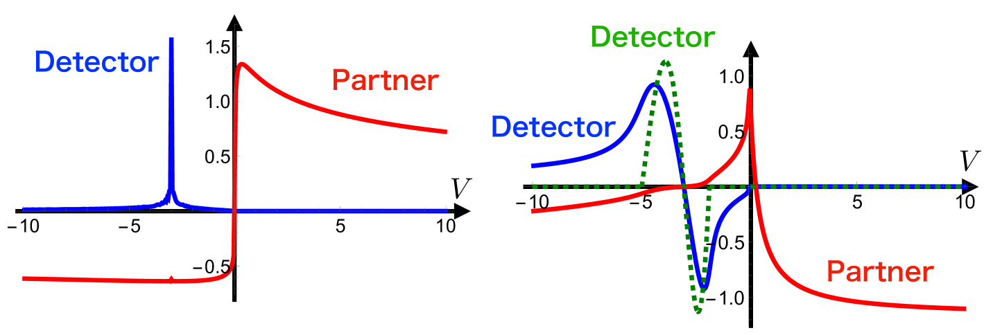
Figure 4: The left panel shows the profile functions $p_{A}^{(1)}(V)$ of detector modes (blue) and its partner mode $p_{P}^{(1)}(V)$ (red) with $a=1,\omega_{-}=0.1,\omega_{+}=1000,V_{A}=-3$. The right panel shows the profile functions $p_{A}^{(2)}(V)$ of detector modes (blue) and its partner mode $p_{P}^{(2)}(V)$ (red) with $L=1$, $\varepsilon=0.138$, $V_{A}=-3$. The green dashed line is the profile function of the detector mode with $\varepsilon=0$. Note that the partner mode is ill-defined with $\varepsilon=0$.

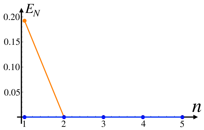
Figure 5: Logarithmic negativity with type 1 detectors ($\omega$-top-hat weighting function) (blue) and with type 2 detectors (the sin-cos profile) (orange). Parameters are $a=1,\omega_{-}=0.1,\omega_{+}=50,V_{A}=-1,L=2\pi/(\omega_{+}-\omega_{-})$, and $\varepsilon=0.02$.

We use logarithmic negativity $E_{N}$ [32, 33, 30] to quantify the entanglement between mode A and mode B:

$$E_{N}:=-\text{min}[\log_{2}(2\tilde{\nu}_{-}),0],$$ (112)

where $\tilde{\nu}_{-}$ is the minimum symplectic eigenvalue of the partially transposed covariance matrix of the bipartite state AB. In Fig. 5, we plot the negativity between local modes as a function of $n$. The integer $n$ determines the separation between local modes according to Eq. (106). The blue line represents entanglement between type 1 detectors (with the $\omega$-top-hat weighting function modes $\{\hat{q}_{A,B}^{(1)},\hat{p}_{A,B}^{(1)}\}$), while orange line represents entanglement between type 2 detectors (the sin-cos type modes $\{\hat{q}_{A,B}^{(2)},\hat{p}_{A,B}^{(2)}\}$). For type 1 detector modes, two detector modes remain separable regardless of their separation, consistent with the general discussion based on the discriminant $D$. In contrast, type 2 detector modes allow entanglement extraction for $n=1$. This occurs as the type 2 detector modes incorporate the creation operator of the Milne mode, rendering our no-go theorem irrelevant. The conditions for successful entanglement extraction are revisited from the perspective of the shape of the partner mode. As shown in Sec. IV, the discriminant $D$ is expressed in terms of the commutators between the canonical operator of the partner mode and the detector mode B. For the chiral field, these commutators can be rewritten in terms of the products of the derivative of the partner profile function and the profile function of the detector mode B, and the discriminant is

$$D =\frac{1}{2}\int dx\,dy\,q^{\prime}_{P}(x)p^{\prime}_{P}(y)\left(-q_{B}(x)p_{B}(y)+p_{B}(x)q_{B}(y)\right).$$ (113)

If the detector mode B is placed at the location where the derivative of the partner profile $q_{P}(x)$ or $p_{P}(x)$ vanishes, then entanglement extraction fails because $D=0$. This expectation is consistent with the partner profiles shown in Fig. 4 and the behavior of the negativity in Fig. 5. Actually, about the location of the detector (the center of the detector profile), the profile of the partner is flat and the derivative of it becomes zero (left panel of Fig. 4), whereas the derivative of the partner profile is nonzero in the right panel of Fig. 4.

VI Conclusion

We revisited Simon’s criterion of entanglement [30] for the bipartite Gaussian states from the perspective of the partner mode by Hotta et al. [22]. Employing this reformulated Simon’s criterion, we observed that the overlap between the spatial profiles of the detector mode B and the spatial profiles (derivative of spatial profiles for the chiral field) of the partner of the detector mode A is necessary for establishing entanglement between A and B. Thus, our clear understanding of the partner mode’s profile—described as “the profile function of the partner mode indicates the location of the complementary information of the detector mode’s entanglement”—is indeed accurate.

It is important to note that the overlap of profile functions does not serve as an equivalent condition to Simon’s criterion. In certain instances, Simon’s criterion can dismiss the potential for entanglement even when the condition of overlap is fulfilled. An instance of such scenarios is the extraction of entanglement utilizing detectors composed of superpositions of the Rindler modes in region I. The partner mode of a single Rindler mode in region I is the Milne mode in region II. Hence, the location of the partner mode is separated from that of the Rindler mode. On the other hand, if we consider the superposition of the Rindler modes in region I, the partner mode is no longer confined in region II and leaks out from the horizon. In this case, another detector mode $\hat{a}_{B}$ defined as the superposition of the Rindler modes in region I can have overlap with the partner mode $\hat{a}_{P}$ of the first detector mode $\hat{a}_{A}$, and entanglement harvesting is expected to be possible by using the detector mode consisting of the Rindler modes in region I. However, our no-go theorem forbids this entanglement harvesting when $\hat{a}_{A}$ and $\hat{a}_{B}$ consist solely of the annihilation operators of the Rindler modes. In contrast, the theorem does not prohibit entanglement harvesting using a detector mode $\hat{a}_{B^{\prime}}$ containing a creation part, that corresponds to squeezing of the mode. Such squeezing can arise in the case that the detector B^′ accelerates with an acceleration different from the Rindler detector A. The entangling/disentangling phenomena between the accelerating detector and the inertial detector [37, 38] may be one example.

The relationship between the Unruh effect and Hawking radiation can be explored through the moving mirror model [31] which mimics Unruh’s shell collapsing model of the black hole collapse [5]. In this framework, it has been shown that Hawking radiation originates from the Milne mode at past null infinity that reflects off at the mirror and ultimately transforms into real particle modes [22, 34, 29]. Hence, by interchanging the roles of the Rindler modes and the Milne modes, the Unruh effect is directly related to Hawking radiation. The detector modes that detect Hawking radiation (real particles at future null infinity) correspond to detector modes consisting of positive frequency Milne mode in past null infinity. By applying the partner formula for the Rindler modes Eq. (85) to Hawking radiation in black hole spacetimes, we find that the partner of the Hawking radiation is not necessarily confined inside of the black hole. This scenario has already been pointed out by [22].

How should we interpret our no-go theorem in the context of black hole evaporation? By applying our no-go theorem to the Milne modes, we find that harvesting is impossible when detector modes consist solely of Milne mode annihilation operators. Since these detector modes correspond to measurements of real particles emitted from a black hole via Hawking radiation, our result implies that no quantum correlations exist between real particles emitted as Hawking radiation if we follow the vacuum fluctuation scenario [35, 31, 22]. Even under Page’s evaporation scenario [36], quantum correlations among (real) Hawking radiation are absent during the early stages of black hole evaporation. It is important to note that vacuum fluctuations do restore quantum correlations even in the early stage of the black hole evaporation, as discussed previously. These correlations can be extracted by exciting the vacuum fluctuation, for example, through the measurement of the localized field (as discussed in Sec. V.4), by using accelerating detectors, or by employing the spatial superposition of detectors [39, 40]. However, for an observer waiting and observing Hawking radiation at infinity, it is impossible to extract entanglement by measuring real Hawking particles that reach him.

Appendix A Introduction of the parametrization

Let us consider two independent oscillator modes $\hat{a}_{A}$ and $\hat{a}_{B}$ embedded in $n$-mode Gaussian modes $\{\hat{b}_{1},\cdots,\hat{b}_{n}\}$:

$$\hat{a}_{A}:=\sum_{i=1}^{n}\left\{\alpha_{i}^{A}\,\hat{b}_{i}+\beta_{i}^{A}(\hat{b}_{i})^{\dagger}\right\},\quad\hat{a}_{B}:=\sum_{i=1}^{n}\left\{\alpha_{i}^{B}\,\hat{b}_{i}+\beta_{i}^{B}(\hat{b}_{i})^{\dagger}\right\},$$ (114)

$$\sum_{i}(|\alpha_{i}^{A}|^{2}-|\beta_{i}^{A}|^{2})=1,\quad\sum_{i}(|\alpha_{i}^{B}|^{2}-|\beta_{i}^{B}|^{2})=1.$$ (115)

Without loss of generality, either of $\hat{a}_{A}$ or $\hat{a}_{B}$ can be rewritten in terms of squeezing of two independent oscillator modes [22]. In this paper, we transform the oscillator mode $\hat{a}_{A}$. $\hat{a}_{A}$ is rewritten as

$$\hat{a}_{A}=\alpha\,\hat{a}_{\tilde{\parallel}}+\gamma\,\hat{a}_{\tilde{\parallel}}^{\dagger}+\delta\,\hat{a}_{\perp}^{\dagger},$$ (116)

where $\hat{a}_{\tilde{\parallel}}$ is the annihilation part of $\hat{a}_{A}$, and $\alpha$ is its normalization:

$$\hat{a}_{\tilde{\parallel}}=\frac{1}{\alpha}\sum_{i=1}^{n}\alpha_{i}^{A}\,\hat{b}_{i},\quad\alpha={\sqrt{\sum_{i=1}^{n}|\alpha_{i}^{A}|^{2}}}.$$ (117)

The parameters $\gamma$, $\delta$, and the annihilation operator $\hat{a}_{\perp}$ are defined as

$$\gamma :=[\hat{a}_{\tilde{\parallel}},\hat{a}_{A}]=\frac{1}{\alpha}\sum_{i=1}^{n}{\left(\alpha_{i}^{A}\right)\left(\beta_{i}^{A}\right)},$$ (118)

$$\delta :=\sqrt{\alpha^{2}-|\gamma|^{2}-1},$$ (119)

$$\hat{a}_{\perp} :=\frac{1}{\delta}\left(\sum_{i=1}^{n}(\beta_{i}^{A})^{*}\,\hat{b}_{i}-\gamma^{*}\,\hat{a}_{\tilde{\parallel}}\right)=\frac{1}{\delta}\sum_{i=1}^{n}\left(\left(\beta_{i}^{A}\right)^{*}-\frac{\gamma^{*}\alpha_{i}^{A}}{\alpha}\right)\hat{b}_{i}.$$ (120)

In this procedure, we extract the component of the creation part of $\hat{a}_{A}$ that is orthogonal to $\hat{a}_{\tilde{\parallel}}$.

This form of $\hat{a}_{A}$ still contains single mode squeezing. To eliminate this, we introduce a new annihilation operator $\hat{a}_{\parallel}$ defined by

$$\hat{a}_{\parallel}:=\cosh\tilde{r}\,\hat{a}_{\tilde{\parallel}}-e^{i\phi}\sinh\tilde{r}\,\hat{a}^{\dagger}_{\tilde{\parallel}},$$ (121)

where the parameters $\tilde{r}$ and $\phi$ are given by

$$\tanh\tilde{r}=-\frac{|\gamma|}{\alpha},\quad\phi=\text{Arg }\gamma.$$ (122)

By solving this relation for $\hat{a}_{\tilde{\parallel}}$ and substituting it into Eq. (116), we obtain

$$\hat{a}_{A}=\cosh r\,\hat{a}_{\parallel}+\sinh r\,\hat{a}^{\dagger}_{\perp}.$$ (123)

where the parameter $r$ is given by

$$\tanh r:=\frac{\delta}{\alpha\cosh\tilde{r}+|\gamma|\sinh\tilde{r}}.$$ (124)

We now perform a basis transformation from $\left\{\hat{b}_{1},\cdots,\hat{b}_{n}\right\}$ to $\left\{\hat{\bar{b}}_{1},\cdots,\hat{\bar{b}}_{n}\right\}$, constructed so that $\hat{\tilde{b}}_{1}=\hat{a}_{\parallel}$ and $\hat{\tilde{b}}_{2}=\hat{a}_{\perp}$. In this new basis, the oscillator mode $\hat{a}_{B}$ can be expressed as

$$\hat{a}_{B}=\sum_{i=1}^{n}\left\{\bar{\alpha}_{i}^{B}\,\hat{b}_{i}+\bar{\beta}_{i}^{B}\left(\hat{b}_{i}\right)^{\dagger}\right\}.$$ (125)

By introducing operators $\hat{a}_{\parallel^{\prime}}$, $\hat{a}_{\perp^{\prime}}$, and the parameter $r_{1}$, the oscillator mode $\hat{a}_{B}$ can be rewritten as

$$\hat{a}_{B}=\cosh r_{1}\,\hat{a}_{\parallel^{\prime}}+\sinh r_{1}\,\hat{a}^{\dagger}_{\perp^{\prime}},$$ (126)

where $\hat{a}_{\parallel^{\prime}},\hat{a}_{\perp}$ are defined as

$$\hat{a}_{\parallel^{\prime}}=\frac{\sum_{i=1}^{n}\bar{\alpha}^{B}_{i}\,\hat{\bar{b}}_{i}}{\sqrt{\sum_{i=1}^{n}|\bar{\alpha}^{B}_{i}|^{2}}},\quad\hat{a}_{\perp^{\prime}}=\frac{\sum_{i=1}^{n}\left(\bar{\beta}^{B}_{i}\right)^{*}\hat{\bar{b}}_{i}}{\sqrt{\sum_{i=1}^{n}|\bar{\beta}^{B}_{i}|^{2}}}.$$ (127)

with

$$\cosh r_{1}=\sqrt{\sum_{i=1}^{n}|\bar{\alpha}^{B}_{i}|^{2}},\quad\sinh r_{1}=\sqrt{\sum_{i=1}^{n}|\bar{\beta}^{B}_{i}|^{2}}.$$ (128)

The oscillator modes $\hat{a}_{\parallel^{\prime}}$, $\hat{a}_{\perp^{\prime}}$ generally do not coincide with $\hat{a}_{\parallel}$, $\hat{a}_{\perp}$. Furthermore, $\hat{a}_{\parallel^{\prime}}$ and $\hat{a}_{\perp^{\prime}}$ is not independent (i.e., $[\hat{a}_{\parallel^{\prime}},\hat{a}_{\perp^{\prime}}^{\dagger}]\neq 0$) in general.

In the following discussion, we assume that coefficients $\bar{\alpha}_{1}^{B}$ and $\bar{\alpha}_{2}^{B}$ are real for simplicity. This assumption does not affect the results concerning quantum entanglement, as complex phase factors can be removed through local mode transformations which do not change entanglement between systems. By using Gram-Schmidt decomposition, the oscillator modes $\hat{a}_{\parallel^{\prime}}$ and $\hat{a}_{\perp^{\prime}}$ can be decomposed as

$$\hat{a}_{\parallel^{\prime}} =\cos\theta_{1}\,\hat{a}_{\parallel}+\sin\theta_{1}\cos\xi_{1}\,\hat{a}_{\perp}+\sin\theta_{1}\sin\xi_{1}\,\hat{a}_{0},$$

$$\hat{a}_{\perp^{\prime}} =\cos\theta_{2}\,\hat{a}_{\parallel}+\sin\theta_{2}\cos\xi_{2}\,\hat{a}_{\perp}+\sin\theta_{2}\sin\xi_{2}\cos\chi\,\hat{a}_{0}+\sin\theta_{2}\sin\xi_{2}\sin\chi\,\hat{a}_{1}.$$

Here, $\hat{a}_{0}$ and $\hat{a}_{1}$ are oscillator modes independent of $\hat{a}_{\parallel}$ and $\hat{a}_{\perp}$, and determined as

$$\hat{a}_{0} \propto\hat{a}_{\parallel^{\prime}}-\left[\hat{a}_{\parallel^{\prime}},\hat{a}_{\parallel}^{\dagger}\right]\hat{a}_{\parallel}-\left[\hat{a}_{\parallel^{\prime}},\hat{a}_{\perp}^{\dagger}\right]\hat{a}_{\perp},$$ (129)

$$\hat{a}_{1} \propto\hat{a}_{\perp^{\prime}}-\left[\hat{a}_{\perp^{\prime}},\hat{a}_{\parallel}^{\dagger}\right]\hat{a}_{\parallel}-\left[\hat{a}_{\perp^{\prime}},\hat{a}_{\perp}^{\dagger}\right]\hat{a}_{\perp}-\left[\hat{a}_{\perp^{\prime}},\hat{a}_{0}^{\dagger}\right]\hat{a}_{0}.$$ (130)

The proportionality factors are determined by normalization conditions:

$$\left[\hat{a}_{0},\hat{a}_{0}^{\dagger}\right]=\left[\hat{a}_{1},\hat{a}_{1}^{\dagger}\right]=1.$$ (131)

Therefore, $\hat{a}_{B}$ can be written as a linear combination of four independent oscillator modes $\hat{a}_{\parallel}$, $\hat{a}_{\perp}$, $\hat{a}_{0}$, $\hat{a}_{1}$

$$\hat{{a}}_{B} =\cosh r_{1}\left(\cos\theta_{1}\,\hat{a}_{\parallel}+\sin\theta_{1}\cos\xi_{1}\,\hat{a}_{\perp}+\sin\theta_{1}\sin\xi_{1}\,\hat{a}_{0}\right)$$

$$+\sinh r_{1}\left(\cos\theta_{2}\,\hat{a}_{\parallel}^{\dagger}+\sin\theta_{2}\cos\xi_{2}\,\hat{a}_{\perp}^{\dagger}+\sin\theta_{2}\sin\xi_{2}\cos\chi\,\hat{a}_{0}^{\dagger}+\sin\theta_{2}\sin\xi_{2}\sin\chi\,\hat{a}_{1}^{\dagger}\right).$$ (132)

Appendix B Proof for more general cases

In this Appendix, we show that our entanglement criterion based on $D$ remains applicable even when the detector mode A includes single-mode squeezing:

$$\hat{a}_{A}:=\cosh\tilde{r}\,\hat{a}_{\tilde{\parallel}}+\sinh\tilde{r}\cos\theta\,\hat{a}_{\tilde{\parallel}}^{\dagger}+\sinh\tilde{r}\sin\theta\,\hat{a}_{\perp}^{\dagger}.$$ (133)

As mentioned in Appendix A, the operator $\hat{a}_{A}$ can be rewritten as

$$\hat{a}_{A}=\cosh r\,\hat{a}_{\parallel}+\sinh r\,\hat{a}_{\perp}^{\dagger},$$ (134)

by performing the local symplectic transformation with an appropriate squeezing parameter $r^{\prime}$:

$$\hat{a}_{\parallel}=\cosh r^{\prime}\,\hat{a}_{\tilde{\parallel}}+\sinh r^{\prime}\,\hat{a}_{\tilde{\parallel}}^{\dagger}.$$ (135)

The partner formula, evaluated in the $\{\hat{a}_{\parallel},\hat{a}_{\perp}\}$ basis, reads:

$$\hat{a}_{P}=\cosh r\,\hat{a}_{\perp}+\sinh r\,\hat{a}_{\parallel}^{\dagger}.$$ (136)

Hence, the discriminant $D$ of entanglement is

$$D :=-\left|\left[\hat{a}_{P},\hat{a}_{B}^{\dagger}\right]\right|^{2}+\left|\left[\hat{a}_{P},\hat{a}_{B}\right]\right|^{2}$$

$$=\frac{-\cosh^{2}r\cos^{2}\theta_{2}+\sinh^{2}r\sin^{2}\theta^{2}\cos^{2}\xi^{2}}{\cosh^{2}r\sinh^{2}r}\sinh^{2}r_{1},$$ (137)

as derived in Sec. III. In that section, we relate this discriminant $D$ to the determinant of the submatrix $V_{AB}$ of the covariance matrix evaluated for the quantum state $|0000\rangle_{\parallel\perp 01}$.

However, the detector mode $\hat{a}_{A}$ in Eq. (133) is naturally defined in terms of annihilation operators $\{\hat{a}_{\tilde{\parallel}},\hat{a}_{\perp}\}$, and we must evaluate the covariance matrix for the quantum state $|0000\rangle_{\tilde{\parallel}\perp 01}$. The submatrix $\tilde{V}_{AB}$ of the covariance matrix evaluated for the quantum state $|0000\rangle_{\tilde{\parallel}\perp 01}$, is given as

$$\tilde{V}_{AB}=\left(\begin{array}[]{cc}\left\langle\left\{\hat{q}_{A},\hat{q}_{B}\right\}\right\rangle_{\tilde{\parallel}\perp 01}&0\\ 0&\left\langle\left\{\hat{p}_{A},\hat{p}_{B}\right\}\right\rangle_{\tilde{\parallel}\perp 01}\end{array}\right)$$ (140)

where the expectation values are computed as

$$\left\langle\left\{\hat{q}_{A},\hat{q}_{B}\right\}\right\rangle_{\tilde{\parallel}\perp 01}=\left(\cosh 2r^{\prime}+\sinh 2r^{\prime}+1\right)\left(\cosh r\cos\theta_{2}+\sinh r\sin\theta_{2}\cos\xi_{2}\right)\sinh r_{1},$$

$$\left\langle\left\{\hat{p}_{A},\hat{p}_{B}\right\}\right\rangle_{\tilde{\parallel}\perp 01}=-\left(\cosh 2r^{\prime}-\sinh 2r^{\prime}+1\right)\left(\cosh r\cos\theta_{2}-\sinh r\sin\theta_{2}\cos\xi_{2}\right)\sinh r_{1}.$$ (141)

Here, we used the independency conditions Eqs. (5) and (6) to eliminate $\theta_{1}$ and $\xi_{1}$. Thus, the determinant of the submatrix $\tilde{V}_{AB}$ of the covariance matrix is computed as

$$\det\tilde{V}_{AB} =-2(\cosh 2r^{\prime}+1)\left(\cosh^{2}r\cos^{2}\theta_{2}-\sinh^{2}r\sin^{2}\theta_{2}\cos^{2}\xi_{2}\right)\sinh^{2}r_{1}$$

$$=-\frac{\sinh^{2}2r}{2}\left(\cosh 2r^{\prime}+1\right)\left(\left|\left[\hat{a}_{P},\hat{a}_{B}^{\dagger}\right]\right|^{2}-\left|\left[\hat{a}_{P},\hat{a}_{B}\right]\right|^{2}\right)$$

$$\equiv\frac{\sinh^{2}2r}{2}\left(\cosh 2r^{\prime}+1\right)D.$$ (142)

Therefore, Simon’s entanglement criterion $\det\tilde{V}_{AB}<0$ once again coincides with the condition $D<0$ for the discriminant $D$.

Appendix C Derivation of the profile function

In this Appendix, we will derive the following profile function representation

$$q(V) =-2\sqrt{2}\operatorname{Im}\left[\int_{0}^{\infty}d\omega\left\{\left(A(\omega)+B^{*}(\omega)\right)\left(\phi_{\omega}^{\text{I}}(V)\right)^{*}+\left(C(\omega)+D^{*}(\omega)\right)\left(\phi_{-\omega}^{\text{II}}(V)\right)^{*}\right\}\right],$$ (143)

$$p(V) =2\sqrt{2}\operatorname{Re}\left[\int_{0}^{\infty}d\omega\left\{\left(A(\omega)-B^{*}(\omega)\right)\left(\phi_{\omega}^{\text{I}}(V)\right)^{*}+\left(C(\omega)-D^{*}(\omega)\right)\left(\phi_{-\omega}^{\text{II}}(V)\right)^{*}\right\}\right],$$ (144)

for the detector local mode given by

$$\hat{a}:=\int_{0}^{\infty}d\omega\left\{A(\omega)\,\hat{a}^{\text{I}}_{\omega}+B(\omega)\left(\hat{a}^{\text{I}}_{\omega}\right)^{\dagger}+C(\omega)\,\hat{a}^{\text{II}}_{\omega}+D(\omega)\left(\hat{a}^{\text{II}}_{\omega}\right)^{\dagger}\right\}.$$ (145)

This discussion is based on [29]. The relation between canonical operators and creation and annihilation operators is given by

$$\hat{Q}=\frac{\hat{a}+\hat{a}^{\dagger}}{\sqrt{2}},\quad\hat{P}=\frac{\hat{a}-\hat{a}^{\dagger}}{\sqrt{2}i}.$$ (146)

Whereas, by using profile functions, the canonical operators can be represented as

$$\hat{Q} =\int_{-\infty}^{\infty}d{V}q(V)\int_{0}^{\infty}d\omega\left\{\partial_{t}\phi^{\text{I}}_{\omega}(V)\,\hat{a}^{\text{I}}_{\omega}+\partial_{t}\phi^{\text{II}}_{-\omega}(V)\,\hat{a}^{\text{II}}_{\omega}+\text{h.c.}\right\},$$ (147)

$$\hat{P} =\int_{-\infty}^{\infty}d{V}p(V)\int_{0}^{\infty}d\omega\left\{\partial_{t}\phi^{\text{I}}_{\omega}(V)\,\hat{a}^{\text{I}}_{\omega}+\partial_{t}\phi^{\text{II}}_{-\omega}(V)\,\hat{a}^{\text{II}}_{\omega}+\text{h.c.}\right\}.$$ (148)

By comparing Eq. (146), Eq. (147), and Eq. (148), profile functions $q_{A}(y),p_{A}(y)$ and weighting functions $A(\omega)$, $B(\omega)$, $C(\omega)$, and $D(\omega)$ are related as

$$\int d{V}q(V)\partial_{t}\phi^{\text{I}}_{\omega}(V) =\frac{A(\omega)+B^{*}(\omega)}{\sqrt{2}},\quad\int d{V}p(V)\partial_{t}\phi_{\omega}^{\text{I}}(V)=\frac{A(\omega)-B^{*}(\omega)}{\sqrt{2}i},$$ (149)

$$\int d{V}q(V)\partial_{t}\phi^{\text{II}}_{\omega}(V) =\frac{C(\omega)+D^{*}(\omega)}{\sqrt{2}},\quad\int d{V}p(V)\partial_{t}\phi_{\omega}^{\text{II}}(V)=\frac{C(\omega)-D^{*}(\omega)}{\sqrt{2}i}.$$ (150)

The canonical commutation relation for the left-moving mode is

$$\left[\hat{\phi}(V),\hat{\Pi}(V^{\prime})\right] =\int_{0}^{\infty}d\omega\left\{\phi^{\text{I}}_{\omega}(V)\left(\partial_{t}\phi^{\text{I}}_{\omega}(V^{\prime})\right)^{*}-\partial_{t}\phi^{\text{I}}_{\omega}(V^{\prime})\left(\phi^{\text{I}}_{\omega}(V)\right)^{*}\right\}$$

$$\hskip 28.45274pt+\int_{0}^{\infty}d\omega\left\{\phi^{\text{II}}_{-\omega}(V)\left(\partial_{t}\phi^{\text{II}}_{-\omega}(V^{\prime})\right)^{*}-\partial_{t}\phi^{\text{II}}_{-\omega}(V^{\prime})\left(\phi^{\text{II}}_{-\omega}(V)\right)^{*}\right\}$$ (151)

$$\equiv\frac{i}{2}\delta\left(V-V^{\prime}\right).$$

Since the mode functions $\phi^{\text{I}}_{\omega}$ and $\phi_{-\omega}^{\text{II}}$ are restricted to $V>0$ and $V<0$, respectively, the following normalization conditions hold:

$$\frac{1}{4}\delta(V-V^{\prime}) =\operatorname{Im}\left[\int_{0}^{\infty}d\omega\,\phi^{\text{I}}_{\omega}(V)\left(\partial_{t}\phi^{\text{I}}_{\omega}(V^{\prime})\right)^{*}\right]\quad(V,V^{\prime}>0),$$ (152)

$$\frac{1}{4}\delta(V-V^{\prime}) =\operatorname{Im}\left[\int_{0}^{\infty}d\omega\,\phi^{\text{II}}_{-\omega}(V)\left(\partial_{t}\phi^{\text{II}}_{-\omega}(V^{\prime})\right)^{*}\right]\quad(V,V^{\prime}<0).$$ (153)

By using these identities, we obtain (143) and (144).

References

- Hawking [1975] S. W. Hawking, Particle Creation by Black Holes, Commun. Math. Phys. 43, 199 (1975), [Erratum: Commun.Math.Phys. 46, 206 (1976)].
- Hawking [1974] S. W. Hawking, Black hole explosions?, Nature 248, 30 (1974).
- Wald [1994] R. M. Wald, Quantum field theory in curved spacetime and black hole thermodynamics (University of Chicago press, 1994).
- Birrell and Davies [1984] N. D. Birrell and P. Davies, Quantum fields in curved space (Cambridge university press, 1984).
- Unruh [1976] W. G. Unruh, Notes on black-hole evaporation, Phys. Rev. D 14, 870 (1976).
- Candelas and Deutsch [1977] P. Candelas and D. Deutsch, On the vacuum stress induced by uniform acceleration or supporting the ether, Proceedings of the Royal Society of London. A. Mathematical and Physical Sciences 354, 79 (1977).
- Fulling and Davies [1976] S. A. Fulling and P. C. Davies, Radiation from a moving mirror in two dimensional space-time: conformal anomaly, Proceedings of the Royal Society of London. A. Mathematical and Physical Sciences 348, 393 (1976).
- Davies and Fulling [1977] P. C. Davies and S. A. Fulling, Radiation from moving mirrors and from black holes, Proceedings of the Royal Society of London. A. Mathematical and Physical Sciences 356, 237 (1977).
- Gibbons and Hawking [1977] G. W. Gibbons and S. W. Hawking, Cosmological event horizons, thermodynamics, and particle creation, Physical Review D 15, 2738 (1977).
- Reznik [2003] B. Reznik, Entanglement from the vacuum, Foundations of Physics 33, 167 (2003).
- Reznik et al. [2005] B. Reznik, A. Retzker, and J. Silman, Violating bell’s inequalities in vacuum, Physical Review A 71, 042104 (2005).
- Benatti et al. [2010] F. Benatti, R. Floreanini, and U. Marzolino, Entangling two unequal atoms through a common bath, Physical Review A 81, 012105 (2010).
- Nambu [2013] Y. Nambu, Entanglement structure in expanding universes, Entropy 15, 1847 (2013).
- Simidzija and Martin-Martinez [2018] P. Simidzija and E. Martin-Martinez, Harvesting correlations from thermal and squeezed coherent states, Physical Review D 98, 085007 (2018).
- Henderson et al. [2018] L. J. Henderson, R. A. Hennigar, R. B. Mann, A. R. Smith, and J. Zhang, Harvesting entanglement from the black hole vacuum, Classical and Quantum Gravity 35, 21LT02 (2018).
- Cong et al. [2019] W. Cong, E. Tjoa, and R. B. Mann, Entanglement harvesting with moving mirrors, JHEP 2019 (6), 1.
- Simidzija and Mart´ın-Mart´ınez [2017] P. Simidzija and E. Martín-Martínez, Nonperturbative analysis of entanglement harvesting from coherent field states, Phys. Rev. D 96, 065008 (2017).
- Gallock-Yoshimura et al. [2021] K. Gallock-Yoshimura, E. Tjoa, and R. B. Mann, Harvesting entanglement with detectors freely falling into a black hole, Physical Review D 104, 025001 (2021).
- Henderson et al. [2022] L. J. Henderson, S. Y. Ding, and R. B. Mann, Entanglement harvesting with a twist, AVS Quantum Science 4 (2022).
- Nambu and Hotta [2023] Y. Nambu and M. Hotta, Analog de sitter universe in quantum hall systems with an expanding edge, Phys. Rev. D 107, 085002 (2023).
- de SL Torres et al. [2023] B. de SL Torres, K. Wurtz, J. Polo-Gómez, and E. Martín-Martínez, Entanglement structure of quantum fields through local probes, Journal of High Energy Physics 2023, 1 (2023).
- Hotta et al. [2015] M. Hotta, R. Schützhold, and W. Unruh, Partner particles for moving mirror radiation and black hole evaporation, Phys. Rev. D 91, 124060 (2015).
- Trevison et al. [2019] J. Trevison, K. Yamaguchi, and M. Hotta, Spatially overlapped partners in quantum field theory, Journal of Physics A: Mathematical and Theoretical 52, 125402 (2019).
- Hackl and Jonsson [2019] L. Hackl and R. H. Jonsson, Minimal energy cost of entanglement extraction, Quantum 3, 165 (2019).
- Yamaguchi et al. [2020] K. Yamaguchi, A. Ahmadzadegan, P. Simidzija, A. Kempf, and E. Martín-Martínez, Superadditivity of channel capacity through quantum fields, Phys. Rev. D 101, 105009 (2020).
- Nambu and Yamaguchi [2023] Y. Nambu and K. Yamaguchi, Entanglement partners and monogamy in de sitter universes, Phys. Rev. D 108, 045002 (2023).
- Trevison et al. [2018] J. Trevison, K. Yamaguchi, and M. Hotta, Pure state entanglement harvesting in quantum field theory, Progress of Theoretical and Experimental Physics 2018, 103A03 (2018).
- Tomitsuka et al. [2020] T. Tomitsuka, K. Yamaguchi, and M. Hotta, Partner formula for an arbitrary moving mirror in 1+ 1 dimensions, Phys. Rev. D 101, 024003 (2020).
- Osawa et al. [2024] Y. Osawa, K.-N. Lin, Y. Nambu, M. Hotta, and P. Chen, Final burst of the moving mirror is unrelated to the partner mode of analog hawking radiation, Physical Review D 110, 025023 (2024).
- Simon [2000] R. Simon, Peres-horodecki separability criterion for continuous variable systems, Physical Review Letters 84, 2726 (2000).
- Carlitz and Willey [1987] R. D. Carlitz and R. S. Willey, Reflections on moving mirrors, Phys. Rev. D 36, 2327 (1987).
- Peres [1996] A. Peres, Separability criterion for density matrices, Physical Review Letters 77, 1413 (1996).
- Horodecki [1997] P. Horodecki, Separability criterion and inseparable mixed states with positive partial transposition, Physics Letters A 232, 333 (1997).
- Wald [2019] R. M. Wald, Particle and energy cost of entanglement of hawking radiation with the final vacuum state, Phys. Rev. D 100, 065019 (2019).
- Wilczek [1993] F. Wilczek, Quantum purity at a small price: Easing a black hole paradox, arXiv preprint hep-th/9302096 (1993).
- Page [1993] D. N. Page, Information in black hole radiation, Phys. Rev. Lett. 71, 3743 (1993).
- Bruschi et al. [2010] D. E. Bruschi, J. Louko, E. Martín-Martínez, A. Dragan, and I. Fuentes, Unruh effect in quantum information beyond the single-mode approximation, Phys. Rev. A 82, 042332 (2010).
- Lin et al. [2008] S.-Y. Lin, C.-H. Chou, and B. L. Hu, Disentanglement of two harmonic oscillators in relativistic motion, Phys. Rev. D 78, 125025 (2008).
- Foo et al. [2020] J. Foo, S. Onoe, and M. Zych, Unruh-dewitt detectors in quantum superpositions of trajectories, Phys. Rev. D 102, 085013 (2020).
- Barbado et al. [2020] L. C. Barbado, E. Castro-Ruiz, L. Apadula, and i. c. v. Brukner, Unruh effect for detectors in superposition of accelerations, Phys. Rev. D 102, 045002 (2020).