Measurement of the inner horizon in the analog of rotating BTZ black holes by an improved photon fluid

Abstract

We study how to include the inner horizon in the analog of rotating black holes using photon fluids. We find that a vortex beam carrying an improved phase can simulate the rotating BTZ black holes experimentally. In the experiment, we develop a new photon fluid model in a graphene/methanol thermal optical solution, and measure the variation of photon fluid velocity with the radial position using a Fourier plane light spot localization method, while also determining the variation of phonon velocity with the same radial position from the optical vortex intensity distribution. The result provides an extension for the application of optical vortex and a potential possibility for the future experimental exploration about the properties of BTZ black holes and even the anti-de Sitter space.

I Introduction

Photon fluids cc2013 , capable of carrying angular momentum, are ideal candidates for analogue gravity and have been used to simulate the rotating black holes vmp2018 . This simulation is achieved at room temperature through the interaction of vortex light with a self-defocusing medium. The self-defocusing medium fm2008 has a nonlinear refractive index directly related to light intensity, which causes the refractive index to exhibit local negative curvature as light propagates through it, thereby influencing the beam itself. From a microscopic perspective, this effect can be understood as a repulsive interaction between photons mediated by atoms, leading to the formation of a “photon fluid” state fpr1992 ; cb1999 ; vwf2016 . Moreover, the propagation of linear excitations (sound waves) in this fluid occurs as if in an effectively curved spacetime determined by the physical properties of the photon fluid. This analogous curved spacetime can be stationary (e.g., a rotating black hole) due to the stability of the vortex with radial flow and the simultaneous existence of the radial and angular flow, whose stability can be ensured by the nonlocally thermo-optic nonlinearity gct2007 ; vrf2015 .

The simulation of a curved spacetime can be traced back to the thought of the analogue gravity put forward in the year of 1981 wgu1981 ; blv2011 . Up to now, it has been realized experimentally in many different physical systems, such as light in a nonlinear medium pkl2008 ; drl2019 , Bose–Einstein condensates (BEC) lis2010 ; ngs2019 , moving water wtl2011 , superconducting quantum system syf2023 , and others. It is worth noting that these analogue systems have typically been limited to (1+1)-dimensional spacetime, often modeling simple structures like Schwarzschild black holes. Along the earlier studies ybz1972 ; tpw2017 in which the physical phenomena occurring in the rotating spacetime were simulated, Vocke et al. vmp2018 presented experimentally a (2+1)-dimensional rotating spacetime with the definite identification of the ergosphere besides the horizon. In their experiment, the rotating analogue black hole was realized by an optical vortex propagating through a self-defocusing medium at room temperature fm2008 ; vmp2018 , where an ergosurface formed, enclosing the internal region from which rotational energy could be extracted bfw2020 .

Since earlier models vmp2018 ; fm2008 could not include the inner horizon (it is noted that the inner horizon was mentioned in the earlier experiment using BEC to simulate the black hole js2014 , but it is essentially different from ours since there is no rotation for the earlier model) and only represented the equatorial slice of the Kerr geometry, it was proposed theoretically czz2023 that a new type of optical vortex should be used to simulate the Bañado-Teitelboim-Zanelli (BTZ) black hole spacetime btz1992 . The BTZ black hole is a solution to Einstein’s field equations in (2+1)-dimensional gravity with a negative cosmological constant. It has some key differences from Schwarzschild or Kerr black holes bhtz1993 ; for instance, it is asymptotically anti-de Sitter rather than asymptotically flat and lacks a curvature singularity at the origin. This makes it a physical platform for exploring the properties of AdS black holes sc1995 , including the thermodynamics, phase transition, etc, when the radiations can be observed in the future. Further, the AdS/CFT correspondence agmo2000 ; ae2015 had been investigated theoretically in the context of analog gravity sh2015 ; bdt2015 ; gsz2015 ; dlt2016 ; gkg2018 . In particular, different types of AdS black holes could correspond to different gravitational theories or CFTs, such as the exotic BTZ black holes tz2013 ; zbc2013 and planar black holes sh2016 . Therefore, experimentally realizing these black holes is crucial for understanding the theory itself and offers further possibilities for exploring them. In this paper, we experimentally realize a class of AdS black holes, namely the BTZ black holes, using vortex beams, which is highly significant not only for the extensive application of the optical vortex, but also for further exploring the AdS/CFT theory in the laboratory.

The structure of the paper is organized as follows. In Section 2, we describe the analogue model of the BTZ black hole and the necessary optical vortex. In Section 3, we present the experimental results and related details for the analogue BTZ black hole. Finally, in Section 4, we give the conclusion.

II The model

In order to simulate a rotating acoustic BTZ black hole, there should be an effective method to form the inner horizon beside that realized in the earlier simulation for the rotating black holes where the event horizon and the ergosphere had been formed. We consider a monochromatic vortex beam with the topological charge $m$ propagating through a nonlinear medium such as a dilute methanol/graphene solution. The evolution of the photon fluid, when interacting with the medium, is governed by the nonlinear Schrödinger equation (NLSE), in which the thermo-optic nonlinearity is represented by the nonlinear change in refractive index, as expressed in vmp2018 ; vrf2015

$$\Delta n=\gamma\int R\left(r-r^{\prime},z-z^{\prime}\right)I(r^{\prime},z^{\prime})dr^{\prime}dz^{\prime},$$ (1)

where $\gamma$ is the nonlinearity coefficient, $z$ is the propagation direction, $I$ is the light intensity, and $R(r,z)$ is the response function, which depends on the nonlocal processes within the medium. When heat diffusion is limited, the nonlocal response function can be approximated as a delta function, a valid assumption in our study, as discussed in Ref. vmp2018 . In partiuclar, the properties of photon fluid formed in the interaction between the light and the medium in the solution is also controlled by the phase and intensity of the incident optical field. The superfluid behavior of photon fluid is crucial for our experiment, which requires that the wavelength of sound modes simulated in the nonlinear medium is much larger than the healing length. Thus, a linear dispersion for these sound modes is guaranteed. At the same time, the healing length cannot too small to ensure the stability of the fluid. So the light has to propagate in the nonlinear medium for at least one oscillation period to guarantee all those requirements mentioned above, which is realized in our experiment. The detailed discussion see Ref. vmp2018 ; vrf2015 .

As in the earlier analyses vmp2018 ; fm2008 ; czz2023 , the photon fluid has a lateral speed gradient distribution which leads to an analogue spacetime structure with the metric as

$$\mathrm{d}s^{2} =(\frac{\rho_{0}}{c_{s}})^{2}[-(c_{s}^{2}-v_{t}^{2})\mathrm{d}t^{2}-2v_{r}\mathrm{d}r\mathrm{d}t$$

$$-2v_{\theta}r\mathrm{d}\theta\mathrm{d}t+dr^{2}+(r\mathrm{d}\theta)^{2}],$$ (2)

where $c_{s}$ is the local speed of sound and is related to the bulk pressure which is derived from the nonlinear interaction. $c_{s}=\frac{c}{n_{0}}\sqrt{\frac{\left|\gamma\right|I}{n_{0}}}$ where $c$ is the light velocity in the vacuum, $n_{0}$ is the linear refractive index of the sample solution, $\gamma$ is the nonlinearity coefficient, and $I$ is the light intensity within the region selected by the pinhole. The terms $v_{r}$ and $v_{\theta}$ represent the radial and tangential velocity components, from which the total velocity is $v_{t}^{2}=v_{r}^{2}+v_{\theta}^{2}$. For the metric (2), it can model a spacetime about a black hole if the region $v_{r}>c_{s}$ exists where anything cannot escape, and it can model a spacetime about the ergosurface of a rotating black hole if the region $v_{t}>c_{s}>v_{r}$ exists where it is impossible for an observer to remain stationary relative to a distant observer. So, it is appropriate to simulate the properties of a rotating black hole, as made in Ref. vmp2018 , but the inner horizon can not be found in their work. Here, we firstly see if the metric (2) can match the BTZ black hole metric in form.

It is not hard to get that the BTZ black hole metric can be simulated by letting czz2023

$$v_{r}=c_{s}\sqrt{1-(-M+\frac{r^{2}}{l^{2}}+\frac{J^{2}}{4r^{2}})},$$ (3)

$$v_{\theta}=c_{s}\frac{J}{2r},$$ (4)

up to the overall factor $(\frac{\rho_{0}}{c_{s}})^{2}$. Here the constants $G=c=1$ are taken. For BTZ black holes, $\Lambda=-\frac{1}{l^{2}}$ is the negative cosmological constant and $l$ is the radius of the anti-de Sitter space. $M$ and $J$ are the mass and angular momentum of the black hole. The positions of the outer ($r_{+}$) and inner ($r_{-}$) horizon of the black hole are determined by $-M+\frac{r^{2}}{l^{2}}+\frac{J^{2}}{4r^{2}}=0$, which leads to the results, $r_{\pm}^{2}=\frac{Ml^{2}}{2}\left(1\pm\sqrt{1-(\frac{J}{Ml})^{2}}\right)$. We may assume without loss of generality that $J\geq 0$ and assume that $Ml\geq J$ to ensure the existence of an event horizon at $r=r_{+}$. The ergosurface is specified at the position $r_{E}=\sqrt{M}l=\sqrt{r_{+}^{2}+r_{-}^{2}}$. In particular, the metric (2) is valid only in the range where the radial velocity $v_{r}=c_{s}\sqrt{1-(-M+\frac{r^{2}}{l^{2}}+\frac{J^{2}}{4r^{2}})}$ is well defined, and this holds for $R_{-}<r_{-}<r_{+}<R_{+}$ with

$$R_{\pm}^{2}=\frac{(1+M)l^{2}}{2}\left[1\pm\sqrt{1-(\frac{J}{(1+M)l})^{2}}\right],$$ (5)

where $R_{\pm}$ represent the boundary that the analogue can be made. Therefore, the acoustic metric realized by the optical vortex can be regarded as the analogue of the BTZ black hole with the nearly perfect match in form up to an overall factor.

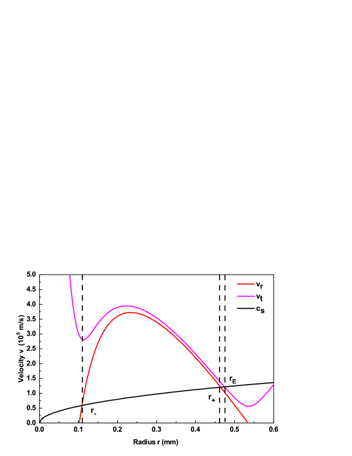
Figure 1: (Color online) The velocities of the fluid as a function of the radius. The parameters are taken according to the actual experimental requirements, i.e. the linear refractive index $n_{0}=1.33$, the nonlinear coefficient $|\gamma|=4.4\times 10^{-11}m^{2}/W$, the power of the laser $p=140$ mW, the beam waist of the laser $\sigma=5$ mm, and the topological charge integer $m=2$.

Then, it is crucial that whether there exists a proper optical vortex which can realize the BTZ spacetime structure. This has been given in Ref. czz2023 by a special Gauss optical vortex with the electric field

$$E_{0}=\sqrt{\rho_{0}(r)}\mathrm{exp}\left(\mathrm{i}m\theta-2\mathrm{i}\pi\left(Ar-B\mathrm{ln}r-Cr^{2}\right)\right),$$ (6)

where $\rho_{0}(r)=\rho_{0}\mathrm{\exp}\left(-\frac{r^{2}}{\sigma^{2}}\right)\tanh^{m/4}(\frac{r}{\sigma})$ takes the super-Gaussian vortex form and $\rho_{0}$, $A$, $B$, $C$ are the constants, and the phase

$$\varphi\left(r\right)=m\theta-2\pi(Ar-B\mathrm{ln}r-Cr^{2}),$$ (7)

which gives the radial and tangential velocities as $v_{r}=\frac{-2\pi c}{kn_{0}}\left(A-\frac{B}{r}-2Cr\right)$ and $v_{\theta}=\frac{cm}{kn_{0}r}$. In the model analogous to the BTZ black hole, the parameters $A$, $B$, and $C$ are subject to specific constraints and they cannot be arbitrarily assigned values to resemble the BTZ black hole. All three parameters must be positive. To ensure the accuracy of the model, it is necessary to precisely adjust the relevant parameters based on the actual structure of the BTZ black hole (as shown in Fig. 1). Specifically, it is essential to ensure that the curves of radial flow velocity and local sound speed have two distinct intersection points, which correspond to the inner and outer horizons of the black hole, respectively. Additionally, the curve of total flow velocity and local sound speed should also have an intersection point, which represents the static boundary. Furthermore, the specific locations of these three intersection points must satisfy certain conditions, i.e. $R_{-}<r_{-}<$ $r_{+}<$ $r_{E}<R_{+}$. Here we take $A=14/2\pi$, $B=1.2/2\pi$, $C=22/2\pi$, and $m=2$ for the topological charge of the optical vortex. The theoretical result for the analogue BTZ black hole is presented in Fig. 1 where the inner and outer horizon and the ergosurface is seen clearly.

III Experimental results

The schematic diagram of the experimental setup is shown in Fig. 2. In the experiment, a continuous wave laser source with a super-Gaussian distribution and a vacuum wavelength of $\lambda=532$ nm is used to generate vortex light. The laser has a maximum power of up to $200$ mW. Initially, the beam is adjusted by passing through a beam expander to increase its diameter. The adjusted super-Gaussian beam then enters a spatial light modulator, where it is modulated to impart the desired phase for generating a required vortex beam. This vortex beam is vertically incident on the input surface of a nonlinear sample. The nonlinear sample is placed in a high-transmittance glass tube with a length of $L=13$ cm, filled with a graphene/methanol solution as the nonlinear medium. The vortex beam output from the nonlinear sample is transmitted through a $4f$ imaging system ($f=75$ mm, the $4f$ system in our experiment is not perfect n4f and see the appendix for the detail) to a pinhole, where it is tracked and scanned. The pinhole has a diameter of $200$ $\mu$m and is mounted on a motorized translation stage that allows for high-precision, three-dimensional directional control. The three-dimensional high-precision motorized translation stage can accurately control the radial scanning of the pinhole along the vortex beam, with a unidirectional movement precision of up to $3$ $\mu$m. Subsequently, a lens with a focal length of $50.8$ mm is used to perform a Fourier transform on the spot selected by the pinhole, converting the frequency distribution of the spot into the spatial distribution. Therefore, the spatial frequency components of the spot can be observed at the focal plane of the lens. After the Fourier transform by the lens, a charge-coupled device (CCD) camera located at the focal plane of the lens records the far-field intensity distribution at the output surface of the nonlinear sample.

In particular, we use an exposure time of 200 $\mu$s to acquire the near-field intensity distribution and to capture the far-field point image by focusing the light onto the Fourier plane using a lens, where the far-field spot is selected through a pinhole. This exposure time is much shorter than the relaxation time from non-equilibrium to equilibrium state in the thermo-optic nonlinear process, and our photos are taken after the system reached a stationary state. Furthermore, because the spatial extent (less than $166$ $\mu$m) of the nonlocal response function is much less than the sound length ($\sim 1$ mm) in our experiment, the nonlocal response function can be approximated as local, which supports the interpretation below Eq. (1).

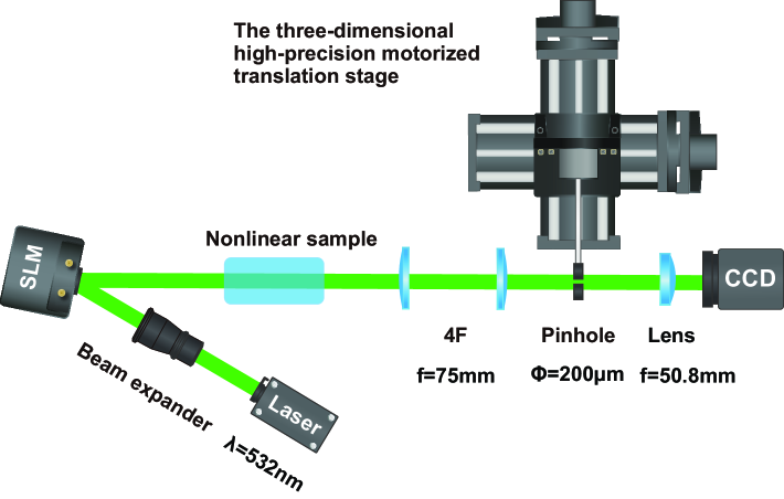
Figure 2: (Color online) Experimental setup: a continuous wave $532$ nm laser beam is emitted into a beam expander for expansion. The expanded beam then enters the SLM (Spatial Light Modulator) to modulate the vortex beam phase as required. The generated vortex beam passes through a $13$ cm long glass tube filled with a graphene/methanol solution and is further expanded using a $4f$ system. The expanded vortex beam then passes through a pinhole (which selects a radial region of the vortex beam and focuses it on the focal plane of the lens), and the spatially resolved far-field is recorded by a CCD camera.

The photon fluid flow can be measured by recording the spatially resolved components $K_{x,\text{ }y}(r)$ in the far field, that is $(v_{x},v_{y})=\frac{c}{n_{0}k_{0}}\left(K_{x},K_{y}\right)$. In the experiment, the pinhole’s position in the vertical direction is fixed at $y=-0.156$ mm. By changing its position in the horizontal direction ($x$) and using the pinhole to track and scan different radial positions of the vortex beam, the location information of the spots captured by the CCD can be used to calculate the flow velocity. The necessary measurement for the phonon velocity is the intensity distribution of the vortex beam after the interaction by taking a photo for the vortex beam in the near field. In particular, it is stressed that the measurement of the light intensity is taken in regions very close to the core and the corresponding results in Fig. 3 are the average values across $x$ axis at the same $y$ position excluding the dark vortex core. The detailed measurement method for the velocities are given in the appendix.

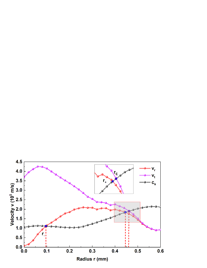
Figure 3: (Color online) Experimental data for the velocities of the fluid and the phonon. The red line represents the radial velocity which leads to the horizons at the intersections with the black line of the phonon speed. The purple line represents the total velocity which gives the position for the ergosurface when it matched with the photon speed. The parameters take the same values as in Fig. 1, but the power of the laser reduces to $70$ mW due to the nonlinear interaction. The measurement error is $\pm 0.003$ unit for radius in the abscissa axis and $\pm 0.02$ unit for velocities in the vertical axis.

Figure 3 shows the velocity curves for the photon fluids and the excited phonons. Acoustic horizons can be identified at the intersections of the fluid velocity (red line) and the phonon velocity (black line) at $r=0.0962$ mm and $r=0.4459$ mm, corresponding to the inner horizon (labeled as $r_{-}$) and the outer horizon (labeled as $r_{+}$), respectively. The ergosurface is larger than the horizons and is located at $r=0.4616$ mm where the total flow velocity (purple line) intersects the phonon velocity (black line), labeled as $r_{E}$. These intersections present evidently the analogous spacetime structure given by the rotating photon fluid after interaction with the nonlinear medium. It is noted that Fig. 3 shows good agreement with the simulation results in Fig. 1, with the specific locations of the three intersections also satisfying the condition ($r_{-}<r_{+}<r_{E}$).

It is able to estimate by the experimental parameters that the analogous spacetime is well within the sonic regime by calculating the angular velocity of the horizon (or the absorbing boundary in the Zel’dovich effect), $\omega_{Z}\simeq\frac{v_{\theta}(r_{+})}{r_{+}}\simeq 1.97\times 10^{8}$ s^-1 which corresponds to phonons with the wavelength $\sim 2\pi c_{s}/\omega_{Z}\simeq 4.15$ mm, or the analog surface gravity $\kappa=\frac{1}{2}\partial_{r}\left(c_{s}^{2}-v_{r}^{2}\right)|_{horizon}\simeq 1.88\times 10^{13}$ ms^-2 which corresponds to phonons with the wavelength $\sim c_{s}^{2}/\kappa\simeq 1.82$ mm. Therefore, we have successfully simulated the acoustic black hole with its structure analogue to a rotating BTZ black hole in (2+1) dimensional spacetime using the vortex beam in the laboratory.

Finally, we have to check whether the analogue is made in the effective regime with the boundary determined by $R_{\pm}$ in the Eq. (5). At first, we express the mass and angular momentum of the analogous black holes as

$$M=\frac{v_{t}^{2}/c_{s}^{2}-1}{1-r_{+}^{2}/r_{E}^{2}},\text{ }J=\frac{2r_{+}v_{\theta}}{c_{s}},$$ (8)

where the radius of anti-de Sitter space given by $r_{E}=\sqrt{M}l$ is used for the expression of the mass. Thus, all the quantities for the black hole are determined by the experimental parameters, which leads to the analogue mass $M\simeq 3.07$, $J\simeq 4.05\times 10^{-4}$ and $l\simeq 2.63\times 10^{-4}$ (up to $c^{2}/G\sim 10^{27}$ kg which is ignored in our discussion). By these, we calculate $R_{+}\simeq 0.52$ mm and $R_{-}\simeq 0.10$ mm, which shows the inner and outer horizons and the ergosurface are well simulated experimentally in the effective regime.

IV Conclusion

In this paper, we experimentally investigate how to use the photon fluid of a vortex beam to simulate a BTZ black hole, presenting an analogy to a rotating black hole with a more complete structure. In the experiment, we recorded videos of the light spot movement through a pinhole during scanning and extracted key frames to capture the changes in the light spot’s position. This allowed us to analyze the radial flow velocity of the vortex beam and the movement speed of phonons more efficiently and in greater detail. By plotting the velocity curves, we clearly identified the positions of the BTZ black hole’s inner horizon, outer horizon, and static boundary, simulating a more complete spacetime structure of the BTZ black hole. This opens a more extensive application of the optical vortex and provides a possibility for further experimental research into the physical properties related to rotating black holes, such as Hawking radiation, Penrose radiation, and even the AdS/CFT correspondence.

V Acknowledgments

This work is supported by National Natural Science Foundation of China (NSFC) with Grant No. 12375057 and the Fundamental Research Funds for the Central Universities, China University of Geosciences (Wuhan).

VI Appendix: Experimental method for measurement of velocities

Here we introduce the method about how to measure the velocities experimentally. As illustrated in the Fig. 2 of the main text. The vortex beam output from the nonlinear sample is modulated in its intensity distribution by the $4f$ system, resulting in the vortex beam shown in the Fig. 4(a), which is the near-field image and is taken when the pinhole and the lens are removed and can be used to measure the light intensity distribution. The interaction between the vortex beam and the nonlinear medium causes the beam’s center to contract. The modulation of the vortex beam by the $4f$ system allows for easier extraction and identification of more detailed spot information from its ring structure. In particular, the $4f$ system is not perfect in our experiment since the first lens is placed at the distance $f$ (=$75$ mm) from the focus but the second lens is placed at the distance a little longer ($80$ mm) from the focus. This amplifies the image of the vortex to observe and measure easier, but this does not alter the crucial structure of the vortex after the nonlinear interaction with the medium. The Fig. 4(b) shows the spot images captured by the CCD after the pinhole selection and focusing onto the lens’s focal plane, which is the far-field image used for the measurement of the fluid velocities.

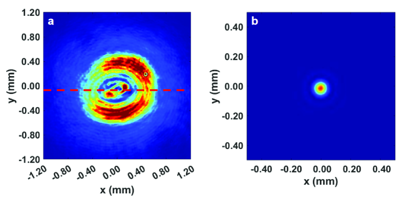
Figure 4: (Color online) The figure (a) presents the vortex beam after expansion by the 4f system. The figure (b) presents the far-field vortex beam at the positions ($K_{x}(x,y=0),K_{y}(x,y=0)$).

Since the velocity is closely related to the nonlinear interaction process, we carefully control the waiting time and exposure time during experiments to ensure accurate measurements. For thermal optical nonlinearity induced by continuous light, the response time depends on the beam intensity (power and focusing radius). For example, a pump beam with a power of $70$ mw, the response time can exceed $1$ second. In our setup, we use a continuous laser source with power stability of more than $99\%$ and allow the vortex beam to interact with the nonlinear medium continuously without a shutter until a stable thermal nonlinear state is achieved. Once stable, we record phase and intensity distributions using a total acquisition time of $5$ seconds, with each frame exposure time controlled to within $200$ $\mu$s to ensure stable and precise measurements.

For the measurement of the sound speed, it is crucial for the methanol to exhibit thermo-optic nonlinearity induced by laser power, characterized by its nonlinear refractive index, with its value as $\gamma=-4.4\times 10^{-11}$ m${}^{\text{2}}$/W. During the preparation of the solution, adding an appropriate amount of nanoscale graphene sheets to methanol can significantly enhance the absorption efficiency of the sample and provide sufficient nonlinearity required for experimental research. The key measurement is the light intensity distribution $I$. In our experiment, multiple regions equal to the pinhole aperture area along the pinhole’s movement path (as indicated by the dashed lines in the Fig. 4(a)) were selected for grayscale integration calculations. Subsequently, we compared the grayscale integration value of each selected region with the total grayscale integration on the CCD detection plane, thereby quantitatively obtaining the power distribution of the selected spots at different positions during the pinhole’s movement. To analyze the radial variation characteristics of the light intensity distribution in detail, the total grayscale integration values of the vortex beam images captured on the CCD plane were calculated. Along the radial direction ($x$-axis), we calculated the grayscale integration value within the pinhole aperture every $0.2$ mm. In our experiment, the camera’s pixel size is $3.45$ micrometers, which means that for the captured spot images, the grayscale integration within an area equal to the pinhole aperture was calculated approximately every $6$ pixels to refine the spatial distribution of light intensity. This series of detailed calculations not only improved the accuracy of the data but also allowed us to closely track the spatial variations in light intensity distribution. Based on these calculations, we successfully plotted the curve of phonon velocity changes.

It is worth noting that when processing light spot images, the grayscale values of the images must be taken into account. Therefore, it is essential to carefully control the camera’s exposure time during image capture. Excessively long exposure times may lead to large areas of overexposure in the vortex beam image, causing the grayscale values in these areas to exceed the maximum threshold of $255$, which can adversely affect the accuracy of the experimental data. Conversely, if the exposure time is too short, the light spot image may not be adequately exposed, resulting in lower grayscale values that fail to accurately represent the true brightness of the light spot. In this case, the captured image will have fewer details, reducing the accuracy of the analysis and compromising the reliability of the experimental results. By properly controlling the exposure time, it is possible to ensure that the light spot images maintain rich detail while accurately reflecting changes in the light spot’s brightness.

For the measurement of the flow speed, we first used a CCD camera to capture the imaging of the vortex beam focused on the focal plane by the lens before measurements, without any pinhole filtering. The peak position at the center of the spot was used as a reference for comparative analysis. Then, using a three-dimensional high-precision motorized translation stage, we performed radial scanning at a speed of $0.2$ mm/s, starting from the edge of the vortex beam. The entire process was video recorded by the CCD camera. We extracted each frame of the spot images from the video, converted the images to grayscale after reading the files, and simplified the analysis process. For the converted grayscale images, we applied image morphology operations to determine the center and area of each region, selecting the region with the largest area as the location of the brightest spot. This allowed us to obtain the position information of the brightness peak at the center of the spot at different radial coordinates of the vortex beam (after selection by the pinhole and focusing by the lens). Based on this position information, the radial flow speed and total flow speed can be calculated.

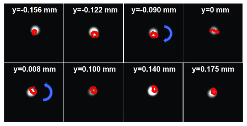
Figure 5: (Color online) The trajectories of the light spots obtained by scanning at different longitudinal positions near the vortex beam center (y=0 mm). Scanning above the vortex beam center is defined as the positive direction, while scanning below the vortex beam center is defined as the negative direction.

It is important to note that in actual optical measurements, due to the zero light intensity at the center of the vortex beam, if the pinhole path coincides with the dark core center of the vortex beam during a surface scan, the light spot trajectory may lose some information as the light intensity inside the pinhole is lower when passing through the dark core. To address this issue, we perform scans in areas very close to the vortex beam’s center. We chose to scan above and below the center of the vortex beam repeatedly. This operation approximates the scenario where the light spot passes through the vortex beam center, allowing for a more accurate acquisition of the required optical information, and can be considered as if the measurement process passes through the optical center. By repeatedly scanning near the vortex beam center, we can minimize the impact of partial loss of the light spot trajectory, thereby improving the accuracy and reliability of the measurements.

As shown in Fig. 5, this is a schematic diagram of the light spot trajectory obtained by scanning at different longitudinal positions near the optical center ($y=0$ mm). Scanning above the vortex beam center is defined as the positive direction, while scanning below the vortex beam center is defined as the negative direction. The direction of movement for the trajectory above the $y=0$ mm position (position greater than $0$ mm) is opposite to that of the trajectory below the $y=0$ mm position (position less than $0$ mm). Complete light spot trajectories can be formed by scanning at certain distances above and below the optical center. However, after the pinhole passes through the dark core region at the center of the vortex beam, part of the light spot trajectory is missing, making it impossible to form a complete closed trajectory. So, selecting a closed trajectory is important for measuring the velocities successfully. Below, we will conduct a detailed analysis of the closed trajectory at the position $y=-0.156$ mm.

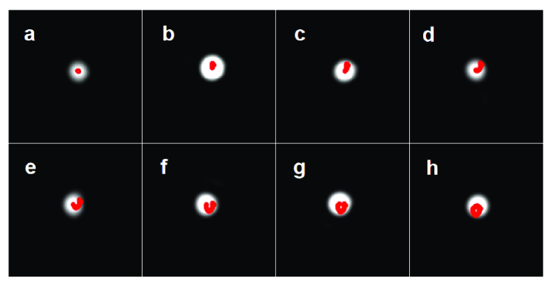
Figure 6: (Color online) The trajectory for the light spot at a distance of y = -0.156 mm from the vortex beam center.

Figure 6 shows the partial light spot trajectory at the position $y=$ $-0.156$ mm. Figs. 6(a) to 6(h) illustrate the movement of the light spot center as the pinhole moves radially along the vortex beam. Before the scanning begins, the center of the light spot selected by the pinhole is located at the position shown in Fig. 6. As the pinhole starts moving radially along the vortex beam, the position of the light spot also begins to change, with the optical center gradually moving in a clockwise direction, eventually forming a closed trajectory. It is important to note that by the end of the scan, the light spot returns to its initial position, coinciding with the light spot center before the scan began, as shown in Fig. 3h.

References

- (1) I. Carusotto and C. Ciuti, Quantum fluids of light, Rev. Mod. Phys. 85, 299 (2013).
- (2) D. Vocke, C. Maitland, and A. Prain, et al, Rotating black hole geometries in a two-dimensional photon superfluid, Optica 5, 2334 (2018).
- (3) F. Marino, Acoustic black holes in a two-dimensional photon fluid, Phys. Rew. A 78, 063804 (2008).
- (4) T. Frisch, Y. Pomeau, and S. Rica, Transition to dissipation in a model of superflow, Phys. Rev. Lett. 69, 1644 (1992).
- (5) R. Y. Chiao and J. Boyce, Bogoliubov dispersion relation and the possibility of superfluidity for weakly interacting photons in a two-dimensional photon fluid, Phys. Rev. A 60, 4114 (1999).
- (6) D. Vocke, K. Wilson, F. Marino, I. Carusotto, E. M. Wright, T. Roger, B. P. Anderson, P. Öhberg, and D. Faccio, Role of geometry in the superfluid flow of nonlocal photon fluids, Phys. Rev. A 94, 013849 (2016).
- (7) N. Ghofraniha, C. Conti, G. Ruocco, and S. Trillo, Shocks in nonlocal media, Phys. Rev. Lett. 99, 043903 (2007).
- (8) D. Vocke, T. Roger, F. Marino, E. M. Wright, I. Carusotto, M. Clerici, and D. Faccio, Experimental characterization of nonlocal photon fluids, Optica 2, 484 (2015).
- (9) W. G. Unruh, Experimental black-hole evaporation? Phys. Rev. Lett. 46, 1351 (1981).
- (10) C. Barceló, S. Liberati, and M. Visser, Analogue gravity, Living Rev. Relativ. 14 3 (2011).
- (11) T. G. Philbin, C. Kuklewicz, S. Robertson, S. Hill, F. König, and U. Leonhardt, Fiber-Optical Analog of the Event Horizon, Science 319, 1367 (2008).
- (12) J. Drori, Y. Rosenberg, D. Bermudez, Y. Silberberg, and U. Leonhardt, Observation of Stimulated Hawking Radiation in an Optical Analogue, Phys. Rev. Lett. 122, 010404 (2019).
- (13) O. Lahav, A. Itah, A. Blumkin, C. Gordon, S. Rinott, A. Zayats, and J. Steinhauer, Realization of a Sonic Black Hole Analog in a Bose-Einstein Condensate, Phys. Rev. Lett. 105, 240401 (2010).
- (14) J. R. M. de Nova, K. Golubkov, V. I. Kolobov, and J. Steinhauer, Observation of thermal Hawking radiation and its temperature in an analogue black hole, Nature 569, 688 (2019).
- (15) S. Weinfurtner, E. W. Tedford, M. C. J. Penrice, W. G. Unruh, and G. A. Lawrence, Measurement of Stimulated Hawking Emission in an Analogue System, Phys. Rev. Lett. 106, 021302 (2011).
- (16) Y. Shi, R. Yang, Z. Xiang, et al, Quantum simulation of Hawking radiation and curved spacetime with a superconducting on-chip black hole, Nat. Commun. 14, 3263 (2023).
- (17) Y. B. Zel’Dovich, Amplification of cylindrical electromagnetic waves reflected from a rotating body, Sov. Phys. JTEP 35, 1085 (1972).
- (18) T. Torres, S. Patrick, A. Coutant, M. Richartz, E. W. Tedford, and S. Weinfurtner, Rotational superradiant scattering in a vortex flow, Nat. Phys. 13 833 (2017).
- (19) M. C. Braidotti, D. Faccio, and E. W. Wright, Penrose superradiance in nonlinear optics, Phys. Rev. Lett. 125, 193902 (2020).
- (20) J. Steinhauer, Observation of self-amplifying Hawking radiation in an analogue black-hole laser, Nat. Phys. 10, 864 (2014).
- (21) L. Chen, H. Zhang, and B. Zhang, An optical analogue for rotating BTZ black holes, Commun. Theor. Phys. 75, 035302 (2023).
- (22) M. Banãdo, C. Teitelboim, and J. Zanelli, Black hole in three-dimensional spacetime, Phys. Rev. Lett. 69, 1849 (1992).
- (23) M. Banãdo, C. Teitelboim, C. Teitelboim, and J. Zanelli, Geometry of the 2+ 1 black hole, Phys. Rev. D 48, 1506 (1993).
- (24) S. Carlip, The (2 + 1)-dimensional black hole, Class. Quantum Grav. 12, 2853 (1995).
- (25) O. Aharony, S. S. Gubser, J. M. Maldacena, H. Ooguri, and Y. Oz, Large N field theories, string theory and gravity, Phys. Rep. 323, 183 (2000).
- (26) M. Ammon and J. Erdmenger, Gauge/Gravity Duality-Foundations and Applications, (Cambridge University Press, Cambridge, UK, 2015)
- (27) S. Hossenfelder, Analog systems for gravity duals, Phys. Rev. D 91, 124064 (2015).
- (28) N. Bili, S. Domazet, and D. Toli, Analog geometry in an expanding fluid from AdS/CFT perspective, Phys. Lett. B 743, 340 (2015).
- (29) X.-H. Ge, J.-R. Sun, Y. Tian, X.-N. Wu, and Y.-L. Zhang, Holographic interpretation of acoustic black holes, Phys. Rev. D 92, 084052 (2015).
- (30) R. Dey, S. Liberati, and R. Turcati, AdS and dS black hole solutions in analogue gravity: The relativistic and nonrelativistic cases, Phys. Rev. D 94, 104068 (2016).
- (31) P. Garza, D. Kabat, and A. van Gelder, Fluid analogs for rotating black holes, Class. Quantum Grav. 35 (2018) 165009.
- (32) P. K. Townsend1 and B. Zhang, Thermodynamics of “Exotic” Banãdos-Teitelboim-Zanelli Black Holes, Phys. Rev. Lett. 110, 241302 (2013).
- (33) B. Zhang, Statistical entropy of a BTZ black hole in topologically massive gravity, Phys. Rev. D 88, 124017 (2013).
- (34) S. Hossenfelder, A relativistic acoustic metric for planar black holes, Phys. Lett. B 752, 13 (2016).
- (35) The non-perfect system causes only a minor modification for the measurement results, which even cannot be presented clearly in the figure of the experimental results. As well-known, when the light goes through the lens, the phase is modulated with a factor, , which leads to a modification for the phase with where is the distance between the focus of the first lens and the second lens, and is the phase that the light carries after going through the second lense which is placed according to the perfect system. When taking the derivative of the phase to obtain the velocity, the modification contributes too small to present in the figure clearly.