Teleportation-based Speed Meter for Precision Measurement
Abstract
We propose a quantum teleportation-based speed meter for interferometric displacement sensing. Two equivalent implementations are presented: an online approach that uses real-time displacement operation and an offline approach that relies on post-processing. Both implementations reduce quantum radiation pressure noise and surpass the standard quantum limit of measuring displacement. We discuss potential applications to gravitational-wave detectors, where our scheme enhances low-frequency sensitivity without requiring modifications to the core optics of a conventional Michelson interferometer (e.g., substrate or coating properties). This approach offers a new path to back-action evasion enabled by quantum entanglement.
Introduction
Precision measurements in cavity optomechanics are fundamentally limited by quantum uncertainties. In free-mass displacement measurements, Heisenberg’s uncertainty principle imposes the standard quantum limit (SQL) [1], arising from a trade-off between measurement precision (associated with position uncertainty) and back-action (associated with momentum uncertainty). Improving measurement precision inevitably leads to an increase in back-action noise.
Various back-action evasion techniques have been developed to mitigate this noise, such as squeezing injection [2, 3, 4, 5, 6], variational readout [6, 7], effective negative-mass systems [8, 9, 10, 11, 12, 13, 14], and optical-spring techniques [15]. Among these, squeezed-state injection has become well-established in gravitational-wave detectors (GWDs). By squeezing a specific quadrature of the vacuum field, one can reduce either position or momentum uncertainty at the expense of the other. The Laser Interferometer Gravitational-wave Observatory (LIGO) has demonstrated an improvement of approximately 3 dB at around 50 Hz, exceeding the SQL [16, 17].
An alternative way to beat the SQL—without relying on squeezing—is to perform quantum non-demolition (QND) measurements of observables that commute with themselves at different times [18, 19]. For a free mass, the momentum operator is one such operator and thus can be monitored in a QND manner that inherently beats the SQL without squeezing. Since momentum is proportional to velocity, such a device that monitors the momentum is often called a speed meter [20, 21].
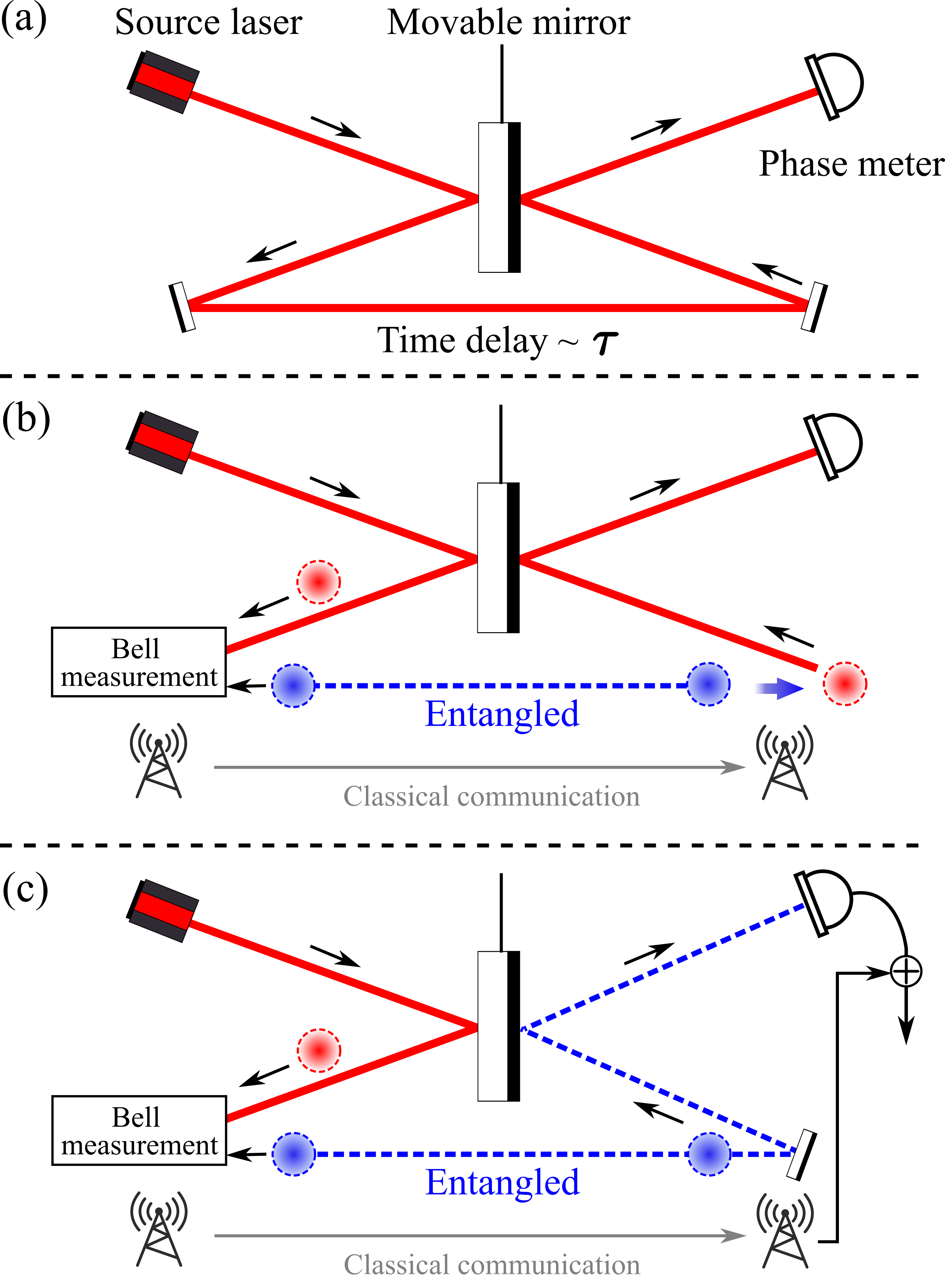
This work proposes a protocol to realize a speed meter through quantum teleportation. The principle of speed measurement is depicted in Fig. 1a; the probe laser is coupled the the object mass twice canceling out the back action of the measurement (see section 4.2. in Ref [22]). For interferometric sensors, previous work realized this coupling using the Sagnac interferometer [23], sloshing cavity mode [24] or manipulation of polarization [25, 26].
Quantum teleportation is widely regarded as a foundational technology for future quantum networks [27, 28] and distributed quantum computing systems [29]. The reliable transfer of unknown quantum states between distant locations enables large-scale quantum communication protocols and significantly enhances data security [30, 31]. Quantum teleportation has also been proposed to extend the baseline of astrophysical telescopes [32].
In this paper, we propose applying quantum teleportation to quantum back-action evasion by means of speed meter. A motivation of our scheme is similar to the conditional or teleportation broadband squeezing approaches proposed in [33, 34], which aim to circumvent technical difficulties in GWDs by exploiting quantum entanglement. Those proposals eliminate the need for large-scale, low-loss, high-finesse filter cavities for broadband squeezing. Our proposal uses quantum entanglement to convert interferometric displacement sensors into speed meters without modifying the substrate or coating properties of the interferometer’s core optics. This approach thus benefits both current [35, 36, 37] and next-generation gravitational-wave detectors [38, 39].
Results
Principle of Speed Measurement
We briefly review the principles of the speed meter. In conventional position measurements, the detector’s sensitivity is ultimately limited by quantum noise, which comprises quantum radiation pressure noise (QRPN) and shot noise. The standard quantum limit (SQL) is given by
| (1) |
where is the angular frequency, is Planck’s constant, and is the mass of the test object. The SQL originates from the non-commutativity of the position operators at different times; that is, the position operator of the test mass at time does not commute with the one at a later time :
| (2) |
Consequently, there is an inherent trade-off between QRPN and shot noise, which prevents both noise sources from being simultaneously reduced.
In contrast, observables that commute at different times can be monitored with arbitrary precision. These are referred to as QND observables. The momentum of a free mirror is one example of a QND observable. For a freely evolving mass, its momentum is proportional to its speed, i.e. , which is why a momentum meter is also called a “speed meter.” However, when the mirror is coupled to a probe such as light, a more careful analysis reveals that the canonical momentum is no longer simply proportional to the speed. Instead, it takes the form
| (3) |
where is the amplitude quadrature of the probe light and represents the optomechanical coupling strength. Nevertheless, it is still possible to reduce the back-action noise below the SQL by exploiting the correlation between the phase and amplitude quadratures of the outgoing field (see Section 2.11 of [40] and Section 4.5.2 of [22]).
An illustration of the light–mirror interaction is provided in Fig. 1a (also see Ref. [22]). Light from the source laser impinges on the front side of the movable mirror, is reflected, and then recycled to the back side of the mirror with a time delay . At the second interaction (at time ), the intensity fluctuations of the light push the mirror in the opposite direction compared to the first interaction (at time ), thereby canceling the initial radiation pressure force. Consequently, the observable measured by the phase meter becomes
| (4) |
where denotes the average velocity of the mirror. Note that when the light interacts with the mirror inside optical cavities, the delay corresponds to the cavity storage time.
Nonreciprocal Coupling via Teleportation
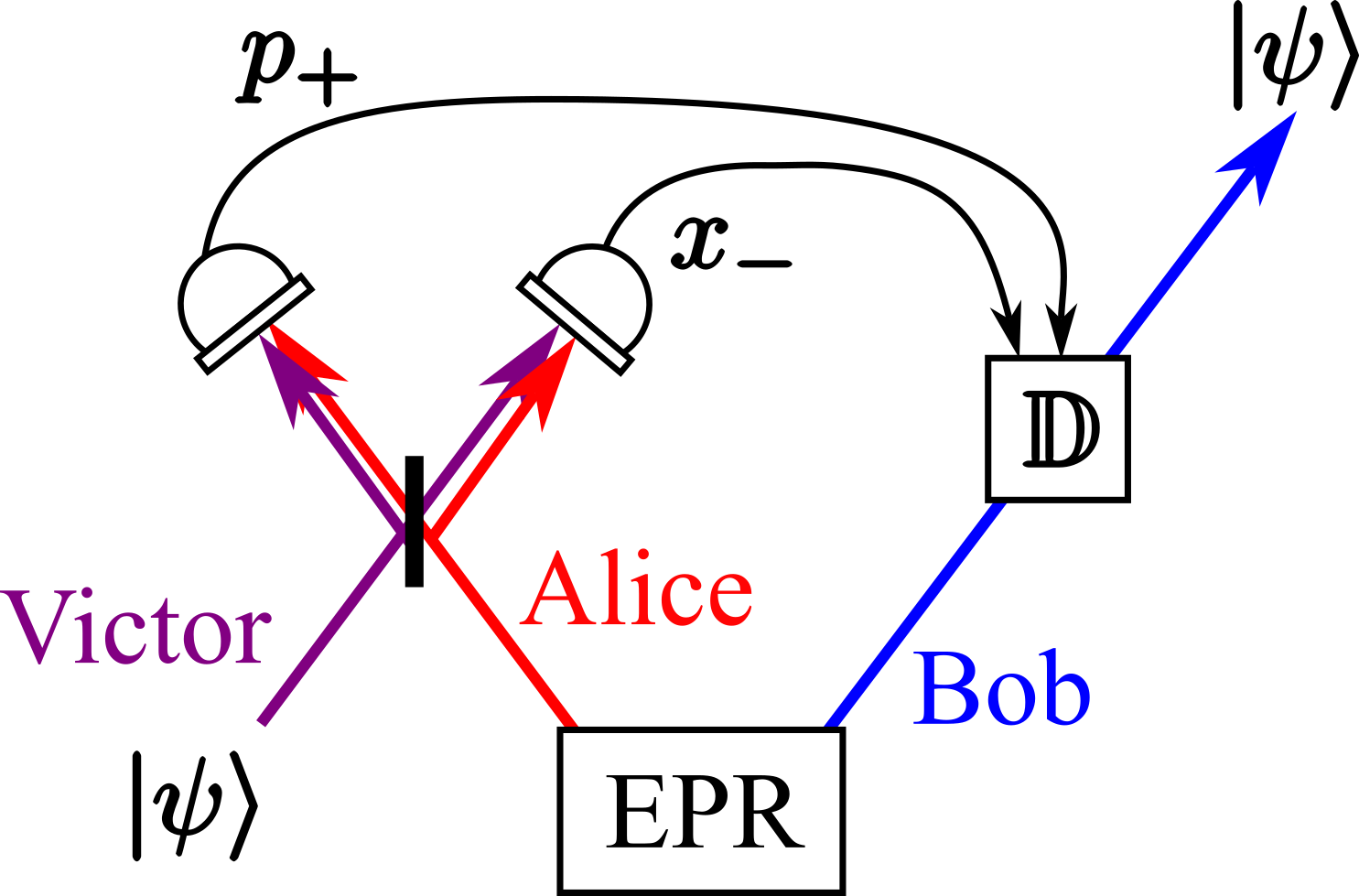
In this section, we discuss how to achieve a speed meter using teleportation. Our teleportation scheme is based on the Braunstein-Kimble protocol [41]. In this protocol, the target state (hereafter referred to as Victor) is teleported from one half of an EPR pair (referred to as Alice) to the other half (referred to as Bob) via the transmission of classical information (see Fig. 2). The transmitted information is obtained from a joint (Bell) measurement performed on Alice and Victor. In an ideal EPR state, two modes are completely correlated, while the individual modes remain completely uncertain (i.e., they exhibit infinite EPR noise). In a conventional homodyne measurement, measuring one observable typically demolishes information about its conjugate; however, when the highly noisy EPR state is mixed with Victor’s state prior to measurement, the measurement reveals no information about Victor’s state. Due to the perfect quantum correlations in an ideal EPR state, only Bob can reconstruct Victor’s state using the classical information from Alice.
In Fig. 1b, an Einstein-Podolsky-Rosen (EPR) entangled pair of photons is distributed to stations on the front and back sides of a mirror, which we denote as Alice and Bob, respectively. The photon that interacts with the mirror on the front side is labeled Victor. Instead of recycling Victor to the mirror’s back side, Alice performs a joint (Bell) measurement on her photon and Victor’s photon. The output of this Bell measurement is a combination of the two quadratures of the input fields necessary for teleportation.
Alice then transmits the measurement results to Bob through classical communication. Bob applies a displacement operation to his photon according to the received data, thereby teleportating Victor’s state to Bob. The teleported state is subsequently directed to the mirror from its back side, where it interacts with the mirror once more. With perfect fidelity of teleportation, this process is therefore equivalent to that depicted in Fig. 1a.
In the following, we first outline the preparation of the initial states for teleportation, then present two equivalent approaches—the online and offline methods, shown in panels (b) and (c) of Fig. 1, respectively. Then, the system dynamics are analyzed using a general Hamiltonian model.
State Preparation and System Dynamics
Throughout this work, we adopt a quadrature representation based on the two-photon formalism [42, 43]. Given that denotes the single-photon annihilation operator of the mode with frequency , the two-photon quadrature amplitudes are defined as
| (5) | ||||
| (6) |
where is the carrier frequency and is the sideband frequency. We denote the fields associated with Victor, Alice, and Bob as
| (7) |
For brevity, we omit the explicit dependence hereafter and introduce subscripts “in” and “out” to denote input and output fields, for example, .
The EPR entanglement, which is a two-mode squeezed vacuum state, is characterized in terms of the quantum spectral density of the four EPR operators for as [44]
| (8) |
where is the squeezing factor. When , the noise spectra of and approach zero, corresponding to the original EPR entanglement [45].
The input field for Victor, (a pure vacuum state, depicted in purple), is injected to mode , interacts with the pump, and then exits as . This field enters the Bell measurement and results in measurement outcomes as follows
| (9) |
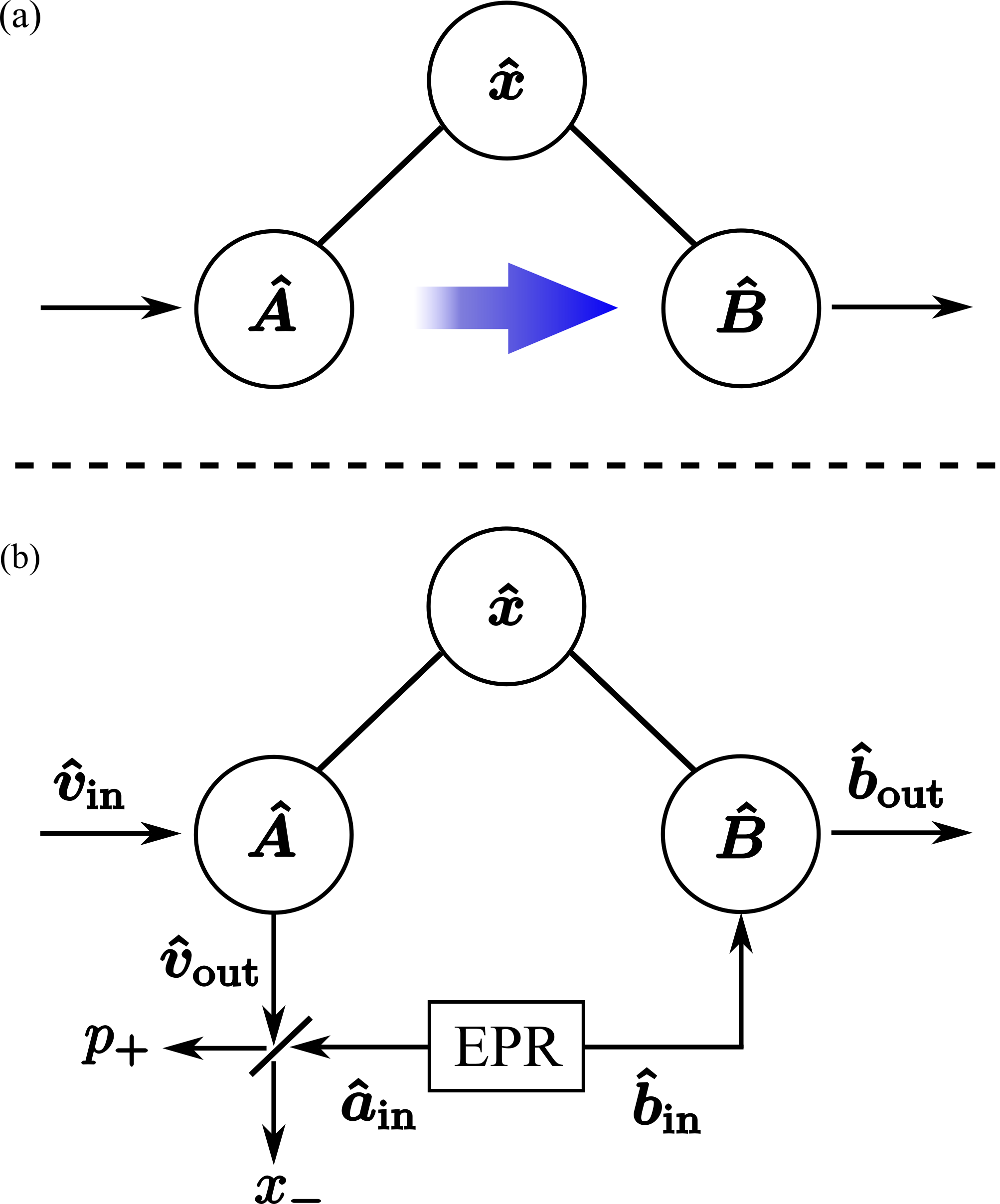
We now describe the system dynamics using an analytic Hamiltonian formalism. Fig. 3a illustrates the mode diagram of the non-reciprocal speed measurement. Two cavity modes, and , are coupled to the position of the oscillator’s mechanical mode . The interaction between and is non-reciprocal: the outgoing field from enters , while the reverse process does not take place. As a result, the input field entering exits from after interacting with the mirror twice. By inverting the sign of the two terms in the Hamiltonian related to the optomechanical interaction, the measurement’s back-action can be effectively canceled out.
The input and output relation of the fields and modes is depicted in Fig. 3b. The Hamiltonian of the system is given by [46, 47]
| (10) | ||||
where is the displacement by external classical force, is the mirror mass, and and denote the natural frequency and momentum operator of the mechanical mode, respectively. is the optomechanical coupling constant between the mechanical and cavity modes. In deriving Eq. (10), we have applied the rotating-wave approximation to ignore the self-evolution of the light modes.
The Heisenberg-Langevin equations of motion in the time domain are thus:
| (11) |
In the Fourier domain and expressed in terms of quadrature operators, these equations become:
| (12) |
where is the cavity’s bandwidth. Here, for , we define the quadratures as
| (13) |
and denote .
The output fields of the two cavity modes are given by
| (14) |
which are the standard input-output relations.
Online Approach
In the “online” approach, the displacement operation is applied to the light field in real time. Here, we first analyze the direct implementation as it provides clearer physical intuition and directly corresponds to the schematic in Fig. 1b. We will later show that this operation can be replaced with post-processing (which we call the “offline” approach).
Bob’s field, denoted as , is displaced based on the Bell measurement’s outcomes and then injected into the mode . The field subsequently couples with , which cancels the back-action, and then emerges as the output as .
The displacement operation, based on the Bell measurement Eq. (9), is expressed as Using Eq. (8), Eq. (LABEL:Eq:displace) can be rewritten as
| (15) |
where the operators have unit variance (i.e., ) and we define .
The output field from mode is then given by where
| (16) | |||
| (17) | |||
| (18) |
Here, is a phase rotation common to both quadratures, and and are the optomechanical coupling factors for the speed meter and the auxiliary field , respectively:
| (19) | ||||
| (20) |
The readout is performed by projecting the outgoing field onto the homodyne vector :
| (21) |
The spectral density for displacement measurement (displacement sensitivity) is then where . The quantum spectral density of the input fields, , is defined by
| (22) |
with (see Refs. [22, 25] for more details). For a readout angle of and in the limit , the displacement sensitivity of the quantum noise–limited interferometer is given by
| (23) |
Offline Approach
The online displacement operation can be replaced by post-processing, which is experimentally easier as it can be implemented “offline”. In this case, the input–output relation can be obtained by setting in Eq. (LABEL:Eq:displace) as: with
| (24) | |||
| (25) | |||
| (26) |
Here, is the optomechanical coupling constant for the position meter:
| (27) |
which satisfies the relation:
| (28) |
For simplicity, in the limit , the measured output (with ) is conditioned by combining it with using Wiener filters and :
| (29) |
The optimal filters are found to be
| (30) |
under which the offline displacement sensitivity in Eq. (29) agrees with the online value in Eq. (23).
Compared to the online approach or ordinary speed meter schemes, the offline approach has the distinct feature that the back-action force acting on the mirror is not actually canceled. In the toy model of Fig. 1c, the back-action force exerted by Victor’s field on the front side of the mirror has no correlation with the force by Bob’s field, so ordinary homodyne detection fails to cancel it. Nevertheless, the back-action is canceled in the eventual sensitivity curve, conditionally erased in post-processing. The key is the Bell measurement, which creates tripartite entanglement among the EPR pair and Victor [41], thereby effectively enabling the cancellation of the back-action force in the offline data.
Sensitivity analysis
In this section, we first analyze the enhancement in sensitivity relative to both a conventional position meter and the standard quantum limit. We then examine the effect of optical losses, which include power losses at the input port, within the arm cavity, and at the output port. Finally, we apply the proposed technique to interferometric gravitational-wave detectors.
Enhancement
A key feature of the speed meter is its optomechanical coupling factor, , which remains constant at low frequencies . Consequently, the speed meter significantly reduces radiation pressure noise. Moreover, since remains constant at low frequencies, the radiation pressure noise can be canceled by exploiting correlations between the amplitude and phase quadratures without requiring frequency-dependent or variational readout (which would otherwise necessitate additional long filter cavities). The optimal homodyne (readout) angle at DC is given by
Thus, with a fixed-angle readout, the sensitivity can beat the SQL in the radiation-pressure–dominated region. In contrast, the coupling constant of the conventional position meter, shown in Eq. (27), exhibits a frequency dependence proportional to .
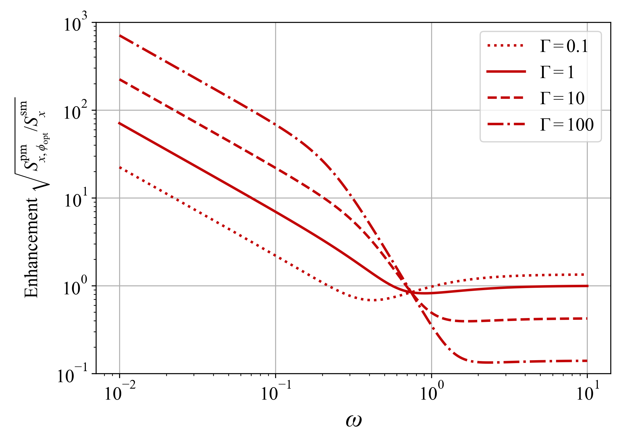
The enhancement factor, in the sensitivity of the speed meter compared to the position meter is given by
| (31) |
where
| (32) |
(for the derivation of the position meter noise , see the supplementary information I). Equation (31) converges to in the limit , indicating that the high-frequency (shot-noise–limited) sensitivities of the speed meter and the position meter coincide when . Fig. 4 shows the enhancement factor for several values of . The enhancement at low frequencies becomes more pronounced as increases, which can be realized by increasing the laser power or reducing the mirror mass.
The enhancement beyond the SQL is quantified as
| (33) |
which is equivalent to the parametrization presented in Ref. [25]. Thus, the speed meter beats the SQL when .
Loss analysis
We now introduce losses to the sensitivity analysis. For the analysis, we focus on the online approach, but we confirmed that the results are equivalent for the offline case. Losses inside the arm cavity introduce extra vacuum noise into the equations of motion:
| (34) |
Here, the loss-induced vacuum fields ( and ) have unit covariance, and is the mode extraction rate due to the power loss.
Additional losses occur in the detection and input optics. The output fields become:
| (35) | ||||
| (36) |
and the input Bob’s field is modified as:
| (37) |
Here , and are the loss-induced vacuum fields with unit covariance. Using the transfer matrices for each field, one can compute the overall displacement sensitivity (see the supplementary information II).
Interferometric gravitational-wave detector
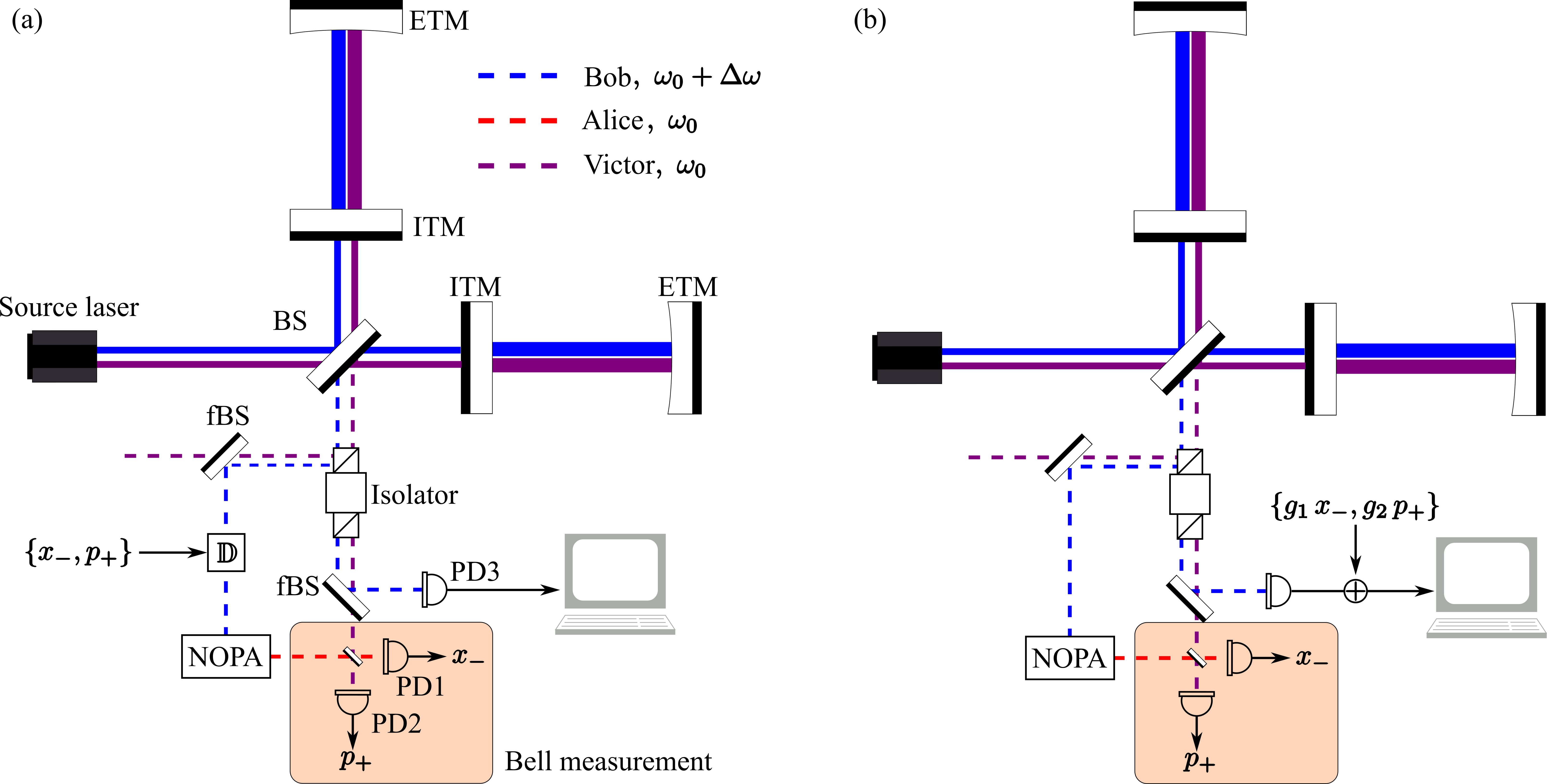
We apply the teleportation-based speed measurement scheme to a LIGO-type gravitational-wave detector and compare its displacement sensitivity to that of a conventional Michelson interferometer operating as a position meter, both using the same total circulating laser power. Panels (a) and (b) of Fig. 5 show the schematics of the online and offline approaches in a Michelson-type interferometer, respectively. The input fields, Bob and Victor, are injected through the Faraday isolator. Alice’s and Victor’s fields share the same frequency, , while Bob’s frequency is slightly detuned to . The pump fields at frequencies and co-resonate in the arm cavities. The beam splitters at the dark port combining the three beams are frequency-dependent; for example, a triangular optical cavity can be used to realize this. The coupling constant is defined as
with the normalized power , where is the total circulating power, is the laser frequency, and is the speed of light. In the online approach, a displacement operation is applied at the dark port, whereas in the offline approach all operations are implemented via post-processing.
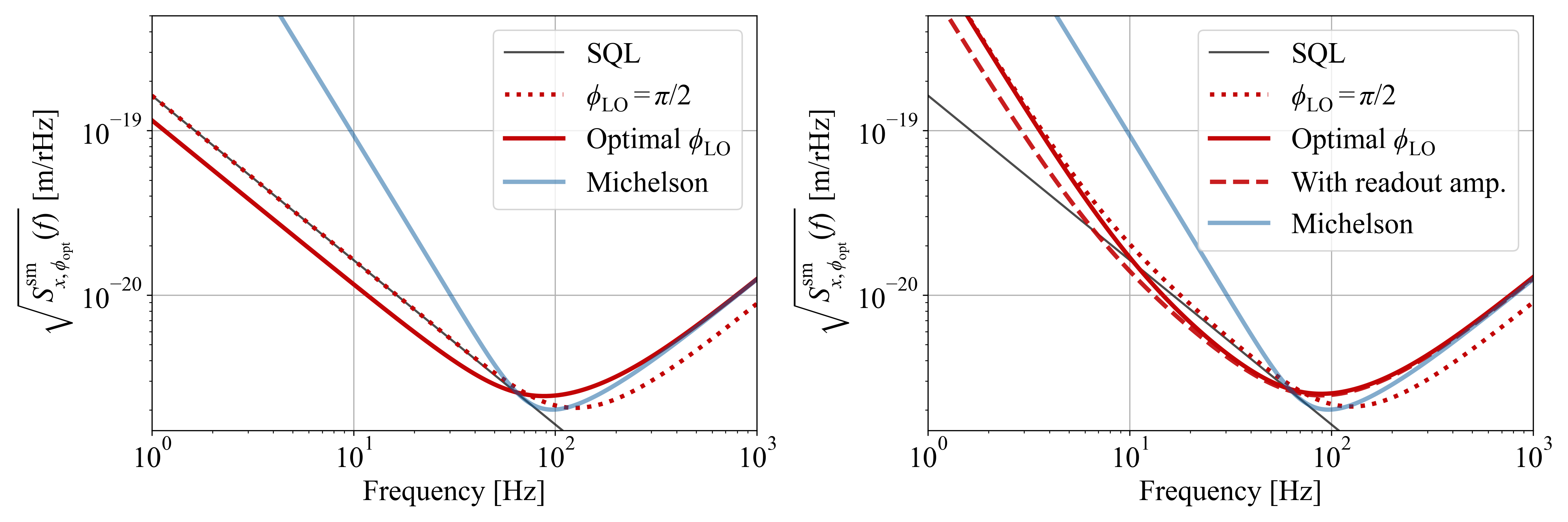
The left panel of Fig. 6 shows the displacement sensitivity curves in the lossy case. The system parameters are chosen to match those in Ref. [25], where the shot-noise–limited sensitivity of the position meter and the speed meter with the optimal homodyne angle are aligned to the same level by setting . At , the low-frequency noise nearly reaches the SQL, whereas using the optimal homodyne angle allows the sensitivity to surpass the SQL. Compared to the position meter, the amplitude sensitivity is improved by approximately one order of magnitude at 8 Hz.
The right panel of Fig. 6 shows the displacement sensitivity curves in the lossy case. Although losses degrade sensitivity, our proposed scheme still yields a considerable enhancement at low frequencies. Below 10 Hz, the sensitivity degrades due to uncorrelated vacuum noise introduced by losses. In our simulation, we assumed 1% input and output losses for each of the three fields and ppm round-trip loss in the arm cavity. The arm loss contributes as the additional damping as . The EPR entanglement is generated with 15 dB of squeezing—beyond which the sensitivity no longer improves because the interferometer losses dominate (note that 15 dB is the generated squeezing level, not the observed level). The low-frequency sensitivity scales as , reflecting the frequency dependence of the radiation pressure by the loss-induced vacuum. Despite the presence of losses, the low-frequency sensitivity remains enhanced, and with the optimal homodyne angle the sensitivity surpasses the SQL.
Discussion
In the online approach, the teleportation works as a frequency converter, which is analogous to the polarization circulator in Ref. [25]. The benefit of using quantum teleportation is that this operation can instead be achieved offline, which is not possible with a classical frequency converter.
When applied to interferometric displacement sensors, our scheme requires no modifications to the core interferometer optics including the coating properties only by altering the dark-port components and introduces a second pump from the bright port (which is similar to the paired carrier interferometry in Ref. [48, 49]). The teleportation-based speed meter needs only two pumping lasers at slightly different frequencies (detuned on the order of MHz). Such two-color lasers can be generated, for example, by using an electro-optic modulator.
The simulation presented omits some experimental details of the teleportation procedure. In the online approach, the physical displacement operation, using a low-transmissivity mirror and coherent laser with modulation [50], may introduce additional losses, making the offline method more favorable in practice.
A major challenge in entanglement-based schemes is to mitigate the noise contribution from input and output losses. In our approach, three detection ports contribute output noise (a threefold effect), while input losses affect both Victor and Bob (a twofold effect). The readout noise can be mitigated by employing a readout amplifier [51, 52, 53, 54]. The dashed curve in the right panel of Fig. 6 shows that readout amplification improves sensitivity in the radiation-pressure–dominated band, compared to that without the amplifier.Readout amplification is crucial not only for the teleportation-based speed meter but also for other multi-color interferometric techniques.
In this article, we propose an alternative speed meter scheme for interferometric displacement sensors based on quantum teleportation. We introduce two equivalent implementations—an online approach and an offline approach—both of which achieve quantum noise reduction below the standard quantum limit (SQL), even in the presence of losses. When applied to interferometric gravitational-wave detectors, the scheme requires no modification to the core interferometer design or to mirror properties such as coatings or substrate materials. This provides a practical route to realizing speed meter operation and improving low-frequency sensitivity.
Acknowledgements.
Research by Y. N. is supported by JSPS Grant-in-Aid for JSPS Fellows Grant Number 23KJ0787 and 23K25901. J.W.G. is supported by the Australian Research Council Centre of Excellence for Gravitational Wave Discovery (Project No. CE170100004 and CE230100016), an Australian Government Research Training Program Scholarship, and also partially by the US NSF grant PHY-2011968. In addition, Y.C. acknowledges the support by the Simons Foundation (Award Number 568762). This work was partially supported by JST ASPIRE (JPMJAP2320).References
- Braginskiǐ [1968] V. B. Braginskiǐ, Classical and Quantum Restrictions on the Detection of Weak Disturbances of a Macroscopic Oscillator, Soviet Journal of Experimental and Theoretical Physics 26, 831 (1968).
- Unruh [1983] W. G. Unruh, in Quantum optics. Experimental gravity, and measurement theory (1983).
- Caves [1981] C. M. Caves, Quantum-mechanical noise in an interferometer, Phys. Rev. D 23, 1693 (1981).
- Bondurant and Shapiro [1984] R. S. Bondurant and J. H. Shapiro, Squeezed states in phase-sensing interferometers, Phys. Rev. D 30, 2548 (1984).
- Jaekel and Reynaud [1990] M. T. Jaekel and S. Reynaud, Quantum limits in interferometric measurements, Europhysics Letters 13, 301 (1990).
- Kimble et al. [2001] H. J. Kimble, Y. Levin, A. B. Matsko, K. S. Thorne, and S. P. Vyatchanin, Conversion of conventional gravitational-wave interferometers into quantum nondemolition interferometers by modifying their input and/or output optics, Phys. Rev. D 65, 022002 (2001).
- Vyatchanin and Zubova [1995] S. Vyatchanin and E. Zubova, Quantum variation measurement of a force, Physics Letters A 201, 269 (1995).
- Julsgaard et al. [2001] B. Julsgaard, A. Kozhekin, and E. S. Polzik, Experimental long-lived entanglement of two macroscopic objects, Nature 413, 400â403 (2001).
- Hammerer et al. [2009] K. Hammerer, M. Aspelmeyer, E. S. Polzik, and P. Zoller, Establishing einstein-poldosky-rosen channels between nanomechanics and atomic ensembles, Phys. Rev. Lett. 102, 020501 (2009).
- Woolley and Clerk [2013] M. J. Woolley and A. A. Clerk, Two-mode back-action-evading measurements in cavity optomechanics, Phys. Rev. A 87, 063846 (2013).
- Tsang and Caves [2010] M. Tsang and C. M. Caves, Coherent quantum-noise cancellation for optomechanical sensors, Phys. Rev. Lett. 105, 123601 (2010).
- Ockeloen-Korppi et al. [2016] C. F. Ockeloen-Korppi, E. Damskägg, J.-M. Pirkkalainen, A. A. Clerk, M. J. Woolley, and M. A. Sillanpää, Quantum backaction evading measurement of collective mechanical modes, Phys. Rev. Lett. 117, 140401 (2016).
- Møller et al. [2017] C. B. Møller, R. A. Thomas, G. Vasilakis, E. Zeuthen, Y. Tsaturyan, M. Balabas, K. Jensen, A. Schliesser, K. Hammerer, and E. S. Polzik, Quantum back-action-evading measurement of motion in a negative mass reference frame, Nature 547, 191â195 (2017).
- Khalili and Polzik [2018] F. Y. Khalili and E. S. Polzik, Overcoming the standard quantum limit in gravitational wave detectors using spin systems with a negative effective mass, Phys. Rev. Lett. 121, 031101 (2018).
- Buonanno and Chen [2002] A. Buonanno and Y. Chen, Signal recycled laser-interferometer gravitational-wave detectors as optical springs, Phys. Rev. D 65, 042001 (2002).
- Yu et al. [2020] H. Yu, L. McCuller, M. Tse, N. Kijbunchoo, L. Barsotti, Mavalvala., et al., Quantum correlations between light and the kilogram-mass mirrors of ligo, Nature 583, 43â47 (2020).
- Jia et al. [2024] W. Jia, V. Xu, K. Kuns, M. Nakano, L. Barsotti, M. Evans, N. Mavalvala, et al., Squeezing the quantum noise of a gravitational-wave detector below the standard quantum limit, Science 385, 1318â1321 (2024).
- Braginsky et al. [1980] V. B. Braginsky, Y. I. Vorontsov, and K. S. Thorne, Quantum nondemolition measurements, Science 209, 547 (1980), https://www.science.org/doi/pdf/10.1126/science.209.4456.547 .
- Braginsky et al. [1995] V. B. Braginsky, F. Y. Khalili, and K. S. Thorne, Quantum Measurement (Cambridge University Press, 1995).
- Braginsky et al. [2000] V. B. Braginsky, M. L. Gorodetsky, F. Y. Khalili, and K. S. Thorne, Dual-resonator speed meter for a free test mass, Phys. Rev. D 61, 044002 (2000).
- Braginsky and Khalili [1990] V. Braginsky and F. Khalili, Gravitational wave antenna with qnd speed meter, Physics Letters A 147, 251 (1990).
- Danilishin and Khalili [2012] S. L. Danilishin and F. Y. Khalili, Quantum measurement theory in gravitational-wave detectors, Living Reviews in Relativity 15, 10.12942/lrr-2012-5 (2012).
- Chen [2003] Y. Chen, Sagnac interferometer as a speed-meter-type, quantum-nondemolition gravitational-wave detector, Physical Review D 67, 10.1103/physrevd.67.122004 (2003).
- Purdue and Chen [2002] P. Purdue and Y. Chen, Practical speed meter designs for quantum nondemolition gravitational-wave interferometers, Phys. Rev. D 66, 122004 (2002).
- Danilishin et al. [2018] S. L. Danilishin, E. Knyazev, N. V. Voronchev, F. Y. Khalili, C. Gräf, S. Steinlechner, J.-S. Hennig, and S. Hild, A new quantum speed-meter interferometer: measuring speed to search for intermediate mass black holes, Light: Science & Applications 7, 11 (2018), arXiv:1702.01029 [gr-qc] .
- Knyazev et al. [2018] E. Knyazev, S. Danilishin, S. Hild, and F. Khalili, Speedmeter scheme for gravitational-wave detectors based on epr quantum entanglement, Physics Letters A 382, 2219 (2018), special Issue in memory of Professor V.B. Braginsky.
- Briegel et al. [1998] H.-J. Briegel, W. Dür, J. I. Cirac, and P. Zoller, Quantum repeaters: The role of imperfect local operations in quantum communication, Phys. Rev. Lett. 81, 5932 (1998).
- Duan et al. [2001] L.-M. Duan, M. D. Lukin, J. I. Cirac, and P. Zoller, Long-distance quantum communication with atomic ensembles and linear optics, Nature 414, 413â418 (2001).
- Gottesman and Chuang [1999] D. Gottesman and I. L. Chuang, Demonstrating the viability of universal quantum computation using teleportation and single-qubit operations, Nature (London) 402, 390 (1999), arXiv:quant-ph/9908010 [quant-ph] .
- Bennett and Brassard [2014] C. H. Bennett and G. Brassard, Quantum cryptography: Public key distribution and coin tossing, Theoretical Computer Science 560, 7â11 (2014).
- Ekert [1991] A. K. Ekert, Quantum cryptography based on bell’s theorem, Phys. Rev. Lett. 67, 661 (1991).
- Gottesman et al. [2012] D. Gottesman, T. Jennewein, and S. Croke, Longer-baseline telescopes using quantum repeaters, Phys. Rev. Lett. 109, 070503 (2012).
- Ma et al. [2017] Y. Ma, H. Miao, B. H. Pang, M. Evans, C. Zhao, J. Harms, R. Schnabel, and Y. Chen, Proposal for gravitational-wave detection beyond the standard quantum limit through EPR entanglement, Nature Physics 13, 776 (2017).
- Nishino et al. [2024] Y. Nishino, S. Danilishin, Y. Enomoto, and T. Zhang, Frequency-dependent squeezing for gravitational-wave detection through quantum teleportation, Phys. Rev. A 110, 022601 (2024).
- Somiya [2012] K. Somiya, Detector configuration of kagraâthe japanese cryogenic gravitational-wave detector, Classical and Quantum Gravity 29, 124007 (2012).
- Acernese et al. [2014] F. Acernese, M. Agathos, K. Agatsuma, D. Aisa, N. Allemandou, et al., Advanced virgo: a second-generation interferometric gravitational wave detector, Classical and Quantum Gravity 32, 024001 (2014).
- Collaboration et al. [2015] T. L. S. Collaboration, J. Aasi, B. P. Abbott, R. Abbott, T. Abbott, M. R. Abernathy, K. Ackley, et al., Advanced ligo, Classical and Quantum Gravity 32, 074001 (2015).
- Hild et al. [2011] S. Hild et al., Sensitivity studies for third-generation gravitational wave observatories, Classical and Quantum Gravity 28, 094013 (2011).
- Abbott et al. [2017] B. P. Abbott, R. Abbott, T. D. Abbott, M. R. Abernathy, et al., Exploring the sensitivity of next generation gravitational wave detectors, Classical and Quantum Gravity 34, 044001 (2017).
- Miao [2010] H. Miao, Exploring macroscopic quantum mechanics in optomechanical devices, Springer Theses (2010).
- Braunstein and Kimble [1998] S. L. Braunstein and H. J. Kimble, Teleportation of continuous quantum variables, Phys. Rev. Lett. 80, 869 (1998).
- Schumaker and Caves [1985] B. L. Schumaker and C. M. Caves, New formalism for two-photon quantum optics. ii. mathematical foundation and compact notation, Phys. Rev. A 31, 3093 (1985).
- Caves and Schumaker [1985] C. M. Caves and B. L. Schumaker, New formalism for two-photon quantum optics. i. quadrature phases and squeezed states, Phys. Rev. A 31, 3068 (1985).
- Duan et al. [2000] L.-M. Duan, G. Giedke, J. I. Cirac, and P. Zoller, Inseparability criterion for continuous variable systems, Phys. Rev. Lett. 84, 2722 (2000).
- Einstein et al. [1935] A. Einstein, B. Podolsky, and N. Rosen, Can quantum-mechanical description of physical reality be considered complete?, Phys. Rev. 47, 777 (1935).
- Law [1995] C. K. Law, Interaction between a moving mirror and radiation pressure: A hamiltonian formulation, Phys. Rev. A 51, 2537 (1995).
- Chen [2013] Y. Chen, Macroscopic quantum mechanics: theory and experimental concepts of optomechanics, Journal of Physics B: Atomic, Molecular and Optical Physics 46, 104001 (2013).
- Rehbein et al. [2008] H. Rehbein, H. Müller-Ebhardt, K. Somiya, S. L. Danilishin, R. Schnabel, K. Danzmann, and Y. Chen, Double optical spring enhancement for gravitational-wave detectors, Phys. Rev. D 78, 062003 (2008).
- Korobko et al. [2015] M. Korobko, N. Voronchev, H. Miao, and F. Y. Khalili, Paired carriers as a way to reduce quantum noise of multicarrier gravitational-wave detectors, Phys. Rev. D 91, 042004 (2015).
- Furusawa et al. [1998] A. Furusawa, J. L. Sørensen, S. L. Braunstein, C. A. Fuchs, H. J. Kimble, and E. S. Polzik, Unconditional quantum teleportation, Science 282, 706 (1998).
- Caves [1982] C. M. Caves, Quantum limits on noise in linear amplifiers, Phys. Rev. D 26, 1817 (1982).
- Knyazev et al. [2019] E. Knyazev, F. Y. Khalili, and M. V. Chekhova, Overcoming inefficient detection in sub-shot-noise absorption measurement and imaging, Opt. Express 27, 7868 (2019).
- Frascella et al. [2021] G. Frascella, S. Agne, F. Y. Khalili, and M. V. Chekhova, Overcoming detection loss and noise in squeezing-based optical sensing, npj Quantum Information 7, 10.1038/s41534-021-00407-0 (2021).
- Kwan et al. [2024] K. M. Kwan, M. J. Yap, J. Qin, D. W. Gould, S. S. Y. Chua, J. Junker, V. B. Adya, T. G. McRae, B. J. J. Slagmolen, and D. E. McClelland, Amplified squeezed states: analyzing loss and phase noise, Classical and Quantum Gravity 41, 215005 (2024).