Reliable and efficient inverse analysis using physics-informed neural networks with distance functions and adaptive weight tuning

Abstract

Physics-informed neural networks have attracted significant attention in scientific machine learning for their capability to solve forward and inverse problems governed by partial differential equations. However, the accuracy of PINN solutions is often limited by the treatment of boundary conditions. Conventional penalty-based methods, which incorporate boundary conditions as penalty terms in the loss function, cannot guarantee exact satisfaction of the given boundary conditions and are highly sensitive to the choice of penalty parameters. This paper demonstrates that distance functions, specifically R-functions, can be leveraged to enforce boundary conditions, overcoming these limitations. R-functions provide normalized distance fields, enabling accurate representation of boundary geometries, including non-convex domains, and facilitating various types of boundary conditions. We extend this distance function-based boundary condition imposition method to inverse problems using PINNs and introduce an adaptive weight tuning technique to ensure reliable and efficient inverse analysis. We demonstrate the efficacy of the method through several numerical experiments. Numerical results show that the proposed method solves inverse problems more accurately and efficiently than penalty-based methods, even in the presence of complex non-convex geometries. This approach offers a reliable and efficient framework for inverse analysis using PINNs, with potential applications across a wide range of engineering problems.

Keywords scientific machine learning, physics-informed neural network, implicit distance function, adaptive weight tuning, inverse analysis, incompressible flow

Article Highlights

The main contributions of our study can be summarized as follows:

• First application of R-function-based distance functions to inverse problems using physics-informed neural networks.

• Synergistic integration of distance functions and adaptive weight tuning for reliable inverse analysis.

• Enhanced accuracy and efficiency in inverse problem solutions across diverse and complex geometries.

1 Introduction

Partial differential equations (PDEs) are of fundamental importance in science and engineering, as they describe the physical laws and behaviors of many real-world phenomena. Obtaining analytical solutions to PDEs is often challenging. Consequently, numerical methods such as the finite difference method, the finite volume method and the finite element method have been studied and developed to solve them numerically. While these methods have successfully addressed many problems, they have limitations, such as the need for grid or mesh generation prior to simulation. Moreover, these methods are primarily focused on forward problems, where the solutions are sought for given parameters and boundary conditions (BCs). In contrast, these methods are not directly applicable to inverse problems, which involve estimating physical parameters or unobserved quantities from scarce and noisy data.

In recent years, neural networks have emerged as an alternative approach for solving PDEs, with the pioneering studies appearing in the 1990s [1, 2, 3, 4]. With recent advancements in computational hardware and the spread of machine learning libraries, neural network-based methods have further gained significant attention across diverse disciplines, not only in computer vision and natural language processing, but also in science and engineering. However, a major challenge associated with neural network-based methods is their lack of explainability and trustworthiness [5, 6]. Such concerns have led to a shift towards the development of models that incorporate prior knowledge, thereby improving their interpretability and reliability compared to purely data-driven methods [7]. This is also the case when applying ML to physical problems, which has led to the emergence of a new research field known as scientific machine learning (SciML) [8]. Several approaches have been proposed to integrate known physical laws into the training process of neural networks. Notable examples include the Physics-Informed Neural Network (PINN) [9], in which the governing PDEs are introduced into the loss function; the Deep Ritz Method [10, 11, 12], where the corresponding energy functional is minimized; and the Variational PINN [13, 14], the Weakly Adversarial Network [15], and the deep mixed residual method [16], which are similar to PINN but relax the regularity of trial solutions by using weak formulations or auxiliary variables. One of the key advantages of PINN and its variants is their flexibility in handling both forward and inverse problems in a unified framework with minimal code modifications. In addition, embedded physical laws serve to effectively constrain the search space of parameters, leading to more accurate solutions and robustness to noisy data [17, 18, 19]. PINNs and variants also reduce the need for large amounts of data, making them suitable for problems with limited data availability [20, 21, 22]. In this regard, PINN can be viewed as a class of Sobolev training networks [23, 24], while one can explicitly introduce an additional regularization [25, 26, 27]. This prior knowledge-based regularization has been effectively utilized in various fields, as demonstrated by Kissas et al. [21] for pressure reconstruction from scarce and noisy medical data, and Sun et al. [28] for airfoil design optimization, to name a few. There are also studies to improve the robustness and approximation capabilities of PINN by introducing architecture modifications [29, 30, 31], basis transformations [32, 33, 34], and domain decompositions [35, 36, 37, 38].

Despite the considerable potential and advancements, the accuracy of PINN solutions is still limited by the treatment of boundary conditions. In practice, many approaches only consider the BCs via the loss function, which we refer to as ‘soft imposition’ of boundary conditions. Although this penalty-based method is relatively easy to implement and has been widely adopted, it can lead to poor approximations if not applied carefully [39]. Potential countermeasures have been proposed, including:

• Increasing the weight of the boundary condition loss to enhance soft imposition effect [10, 40, 41]

• Utilizing multiple networks, each learning the prescribed BCs and the governing PDEs separately [42, 43, 44]

• Enforcing boundary conditions using distance functions to the boundary [2, 39, 45, 46]

For methods (1) and (2), however, the accuracy of the solution is heavily dependent on the choice of the weight (penalty parameter) and the optimization method. In particular, for method (1), several studies have proposed adaptive weight tunings based on statistics or norm of backpropagated gradients [24, 30, 47], or Neural Tangent Kernel theory [48, 49]. Nonetheless, including method (2), these approaches only provide approximations, and therefore the resulting solutions are not guaranteed to satisfy the given BCs. Method (3), on the other hand, is independent of the optimizer or approximator, and is the focus of this paper, referred to as ‘hard imposition’. In this method, the approximate solution is derived by projecting the output of the neural network onto the space that exactly satisfies the boundary conditions. This transformation is performed by using distance functions (in a Euclidean sense), which is constructed based on the theory of R-functions [50, 51, 52]. R-functions are a class of functions to encode logical operations into real-valued functions, and have been utilized in geometric modeling [52, 53, 54]. While the application of R-function-based distance functions to numerical and machine learning methods has been explored for forward problems  [55, 56, 57, 46, 58], their use in inverse problems with PINN has not been fully investigated. In this paper, we extend the method discussed in [59, 51, 52, 46, 58] to address inverse problems using PINN, while also applying an adaptive weight tuning [47]. To the best of our knowledge, this is the first study to apply R-function-based distance functions to inverse problems using PINNs. We demonstrate the effectiveness of this approach through numerical experiments, and show that the proposed method can solve inverse problems more accurately and efficiently than the conventional penalty-based method. The remainder of this paper is organized as follows. In Section 2, we provide an overview of the physics-informed neural network (PINN) and describe the properties of the R-function-based distance function. Next, we discuss how to apply the distance function to enforce boundary conditions in PINN, and introduce an adaptive weight tuning along with the technique to ensure the reliability of inverse analysis using PINN. Consequently, in Section 3, we present a series of numerical experiments to evaluate the performance of the proposed method. Finally, we conclude the paper in Section 4, highlighting the significance of our work.

2 Methods

2.1 Physics-informed neural network

For the sake of clarity, we first provide a brief overview of the physics-informed neural network (PINN). Consider the following boundary value problem of the Poisson equation as a model problem:

$$-\nabla^{2}u =f \quad\text{in}\quad\Omega,$$ (1)

$$u =g_{D} \quad\text{on}\quad\Gamma_{D},$$ (2)

$$\bm{n}\cdot\nabla u =g_{N} \quad\text{on}\quad\Gamma_{N},$$ (3)

where $\Omega\subset\mathbb{R}^{d}$ is an open, bounded domain, and $\Gamma=\partial\Omega$ denotes its boundary ($\Gamma=\bar{\Gamma}_{D}\cup\bar{\Gamma}_{N}$, $\Gamma_{D}\cap\Gamma_{N}=\emptyset$, $\Gamma_{D}\neq\emptyset$). Here, $\bm{n}$ represents the outward unit normal vector on $\Gamma$, and $f:\Omega\to\mathbb{R}$, $g_{D}:\Gamma_{D}\to\mathbb{R}$, and $g_{N}:\Gamma_{N}\to\mathbb{R}$ are given functions. The objective is to find the solution $u:\Omega\to\mathbb{R}$ that satisfies Equations (1)–(3).

Following [9], we proceed by approximating the solution $u(\bm{x})$ with a multi-layer perceptron (MLP) $\hat{u}(\bm{x};\bm{\theta})$ [60, 61], where $\bm{\theta}$ denotes the set of trainable parameters. Given an input $\mathbf{x}\in\mathbb{R}^{f^{(0)}}$ and an output $\hat{\mathbf{y}}\in\mathbb{R}^{f^{(L)}}$, the forward pass $\mathbf{z}^{(l)}\in\mathbb{R}^{f^{(l)}}(l=1,\ldots,L)$ is given by:

$$\mathbf{z}^{(l)}=\sigma^{(l)}\left(\mathbf{W}^{(l)}\mathbf{z}^{(l-1)}+\mathbf{b}^{(l)}\right),$$ (4)

where $\mathbf{z}^{(0)}=\mathbf{x}$ and $\mathbf{z}^{(L)}=\hat{\mathbf{y}}$. $\sigma^{(l)}(\cdot)$ is the element-wise nonlinearity, and $\mathbf{W}^{(l)}\in\mathbb{R}^{f^{(l)}\times f^{(l-1)}}$ and $\mathbf{b}^{(l)}\in\mathbb{R}^{f^{(l)}}$ represent the learnable weights and biases, respectively, with $\bm{\theta}={\mathbf{W}^{(l)},\mathbf{b}^{(l)}}_{l=1}^{L}$. In this context, $\mathbf{x}$ corresponds to the spatial coordinates $\bm{x}$, and $\hat{\mathbf{y}}$ represents the approximate solution $\hat{u}$. PINN is trained by minimizing the following loss function:

$$\mathcal{L}(\bm{\theta})=\mathcal{L}_{\text{PDE}}(\bm{\theta})+\lambda_{\text{BC}}\mathcal{L}_{\text{BC}}(\bm{\theta})+\lambda_{\text{Data}}\mathcal{L}_{\text{Data}}(\bm{\theta}),$$ (5)

where each of the terms is evaluated via (quasi-)Monte Carlo approximation (e.g., [62]):

$$\begin{split}\mathcal{L}_{\text{PDE}}&=\int_{\Omega}\left|-\nabla^{2}\hat{u}(\bm{x};\bm{\theta})-f(\bm{x})\right|^{2}\,d\bm{x}\\ &\simeq\frac{1}{N_{\text{PDE}}}\sum_{i=1}^{N_{\text{PDE}}}\left|-\nabla^{2}\hat{u}(\bm{x}_{i};\bm{\theta})-f(\bm{x}_{i})\right|^{2},\end{split}$$ (6)

$$\begin{split}\mathcal{L}_{\text{BC}}&=\int_{\Gamma_{D}}\left|\hat{u}(\bm{x};\bm{\theta})-g_{D}(\bm{x})\right|^{2}\,d\bm{x}+\int_{\Gamma_{N}}\left|\bm{n}\cdot\nabla\hat{u}(\bm{x};\bm{\theta})-g_{N}(\bm{x})\right|^{2}\,d\bm{x}\\ &\simeq\frac{1}{N_{\text{DBC}}}\sum_{i=1}^{N_{\text{DBC}}}\left|\hat{u}(\bm{x}_{i};\bm{\theta})-g_{D}(\bm{x}_{i})\right|^{2}+\frac{1}{N_{\text{NBC}}}\sum_{i=1}^{N_{\text{NBC}}}\left|\bm{n}\cdot\nabla\hat{u}(\bm{x}_{i};\bm{\theta})-g_{N}(\bm{x}_{i})\right|^{2},\end{split}$$ (7)

$$\begin{split}\mathcal{L}_{\text{Data}}&=\int_{\Omega}\left|\hat{u}(\bm{x};\bm{\theta})-u_{\text{Data}}(\bm{x})\right|^{2}\,d\bm{x}\\ &\simeq\frac{1}{N_{\text{Data}}}\sum_{i=1}^{N_{\text{Data}}}\left|\hat{u}(\bm{x}_{i};\bm{\theta})-u_{\text{Data}}(\bm{x}_{i})\right|^{2}.\end{split}$$ (8)

Here, $\lambda_{\text{BC}},\lambda_{\text{Data}}\in\mathbb{R}_{\geq 0}$ are weights (penalty parameters) to control the contributions of boundary conditions and observed data to the loss function. The terms $\mathcal{L}_{\text{PDE}}$, $\mathcal{L}_{\text{BC}}$, and $\mathcal{L}_{\text{Data}}$ represent the loss functions associated with the PDE residual, BC, and observed data, respectively. For forward problems, $\lambda_{\text{Data}}$ can be set to zero, whereas for inverse problems, it is assigned a positive value to reflect the observed data. The penalty parameter $\lambda_{\text{BC}}$ is often set to a large value to better propagate the effects of boundary conditions [10, 41, 63]. These weights may be predefined as fixed constants or adaptively adjusted during the training process [24, 30, 47, 49, 31].

2.2 R-function-based distance function

Let $\Phi(\bm{x})$ be the exact distance function (EDF) from a point $\bm{x}\in\Omega$ to the boundary $\Gamma=\partial\Omega$, and $\phi(\bm{x})$ represent the approximate distance function (ADF). By definition, $\Phi$ satisfies the following properties [64]:

• $\Phi(\bm{x})=0\quad\left(\bm{x}\in\Gamma\right)$

• $\partial_{\bm{\nu}}\Phi(\bm{x})=1\quad\left(\bm{x}\in\Gamma\right)$

• $\partial_{\bm{\nu}}^{M}\Phi(\bm{x})=0\quad\left(\bm{x}\in\Gamma,M\in\mathbb{Z}_{\geq 2}\right)$

where $\bm{\nu}$ is the inward unit normal vector on $\Gamma$ ($\bm{\nu}=-\bm{n}$). Since $\phi$ is an approximation of $\Phi$, it is desirable that it possesses similar properties. Specifically, $\phi$ is required to satisfy properties (A) and (B) as $\Phi$ does, while property (C) is relaxed to a finite order.

• $\phi(\bm{x})=0\quad\left(\bm{x}\in\Gamma\right)$

• $\partial_{\bm{\nu}}\phi(\bm{x})=1\quad\left(\bm{x}\in\Gamma\right)$

• $\partial_{\bm{\nu}}^{k}\phi(\bm{x})=0\quad\left(\bm{x}\in\Gamma,k=2,\ldots,m\in\mathbb{Z}_{\geq 2},\text{for some finite }m\right)$

Such a function $\phi$ is said to be normalized to the $m$-th order or an $m$-th order approximation of $\Phi$ [51, 64]. In the following, we denote $\phi=\phi^{(m)}$ to emphasize the order of normalization, if necessary.

2.2.1 Distance to a line segment

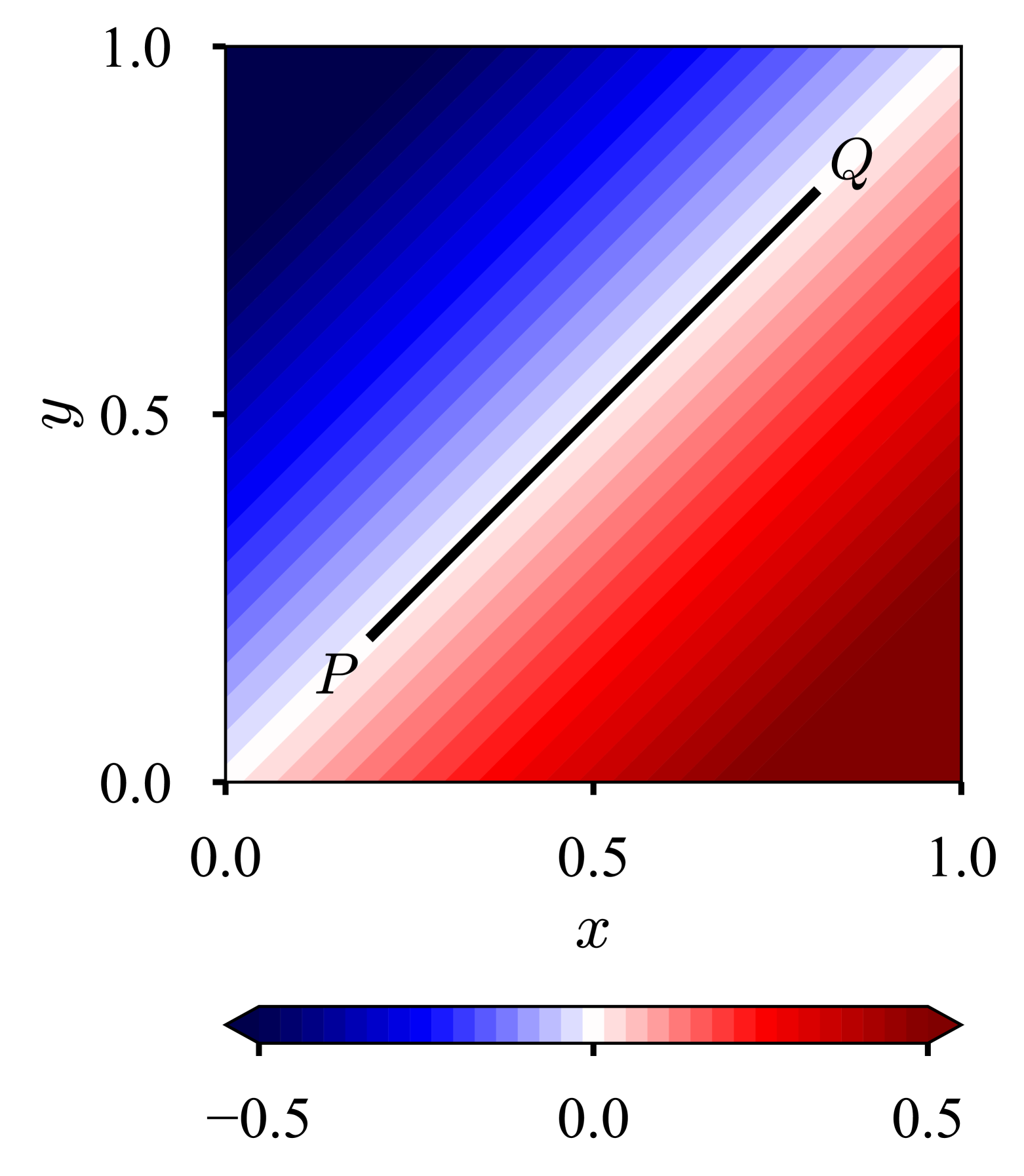
(a) SDF, $s_{PQ}$

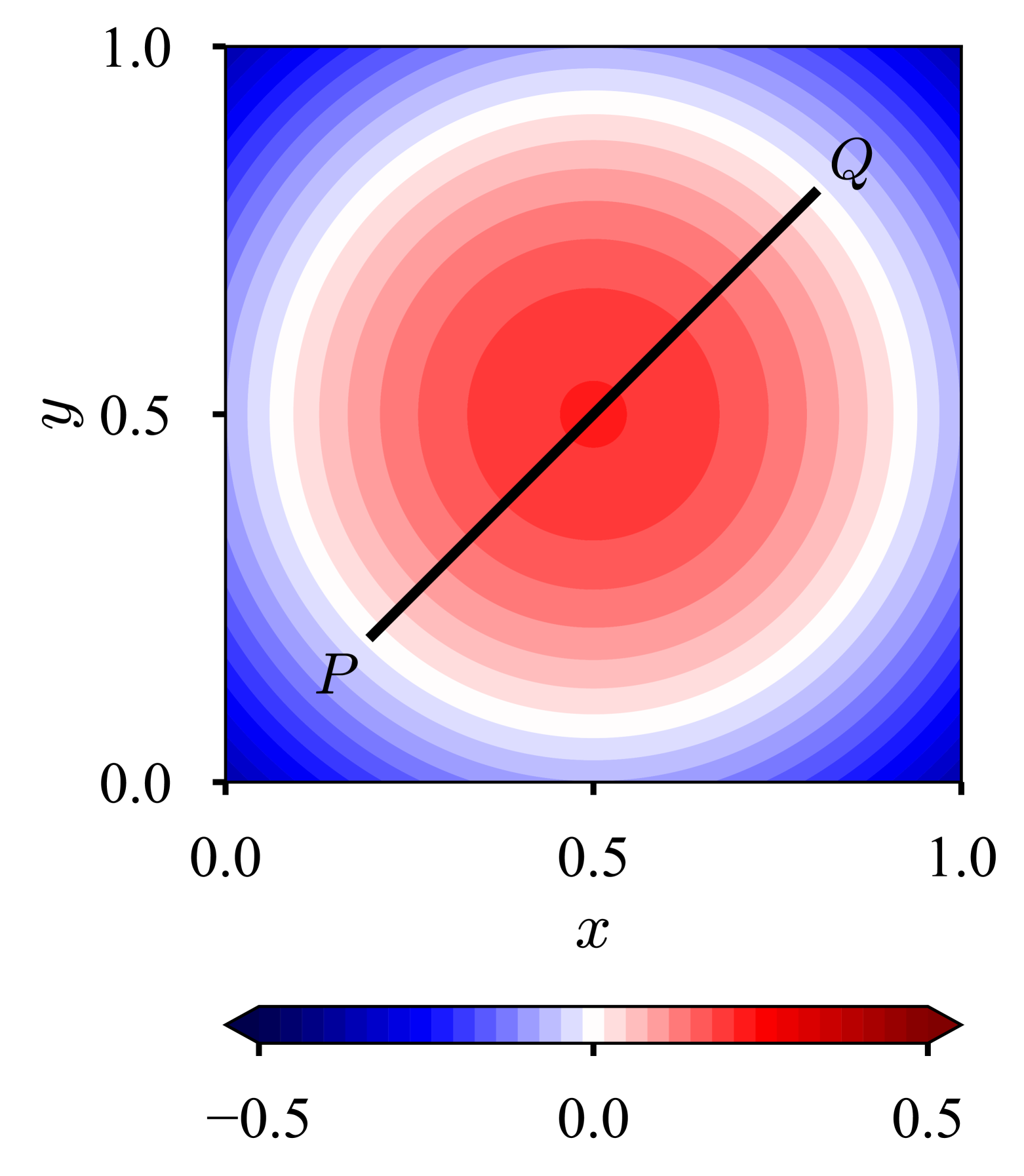
(b) TF, $t_{PQ}$

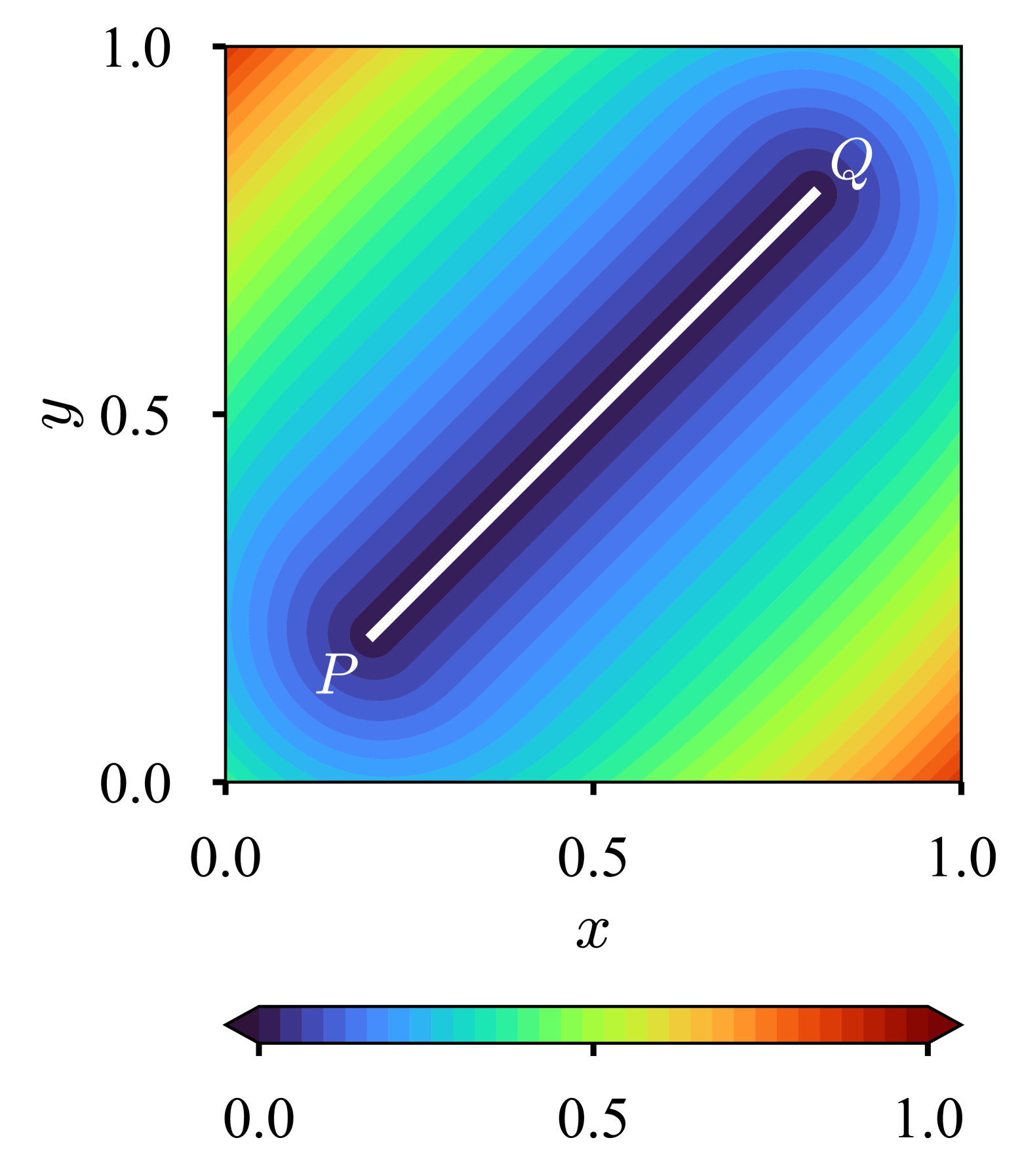
(c) ADF, $\phi_{PQ}$

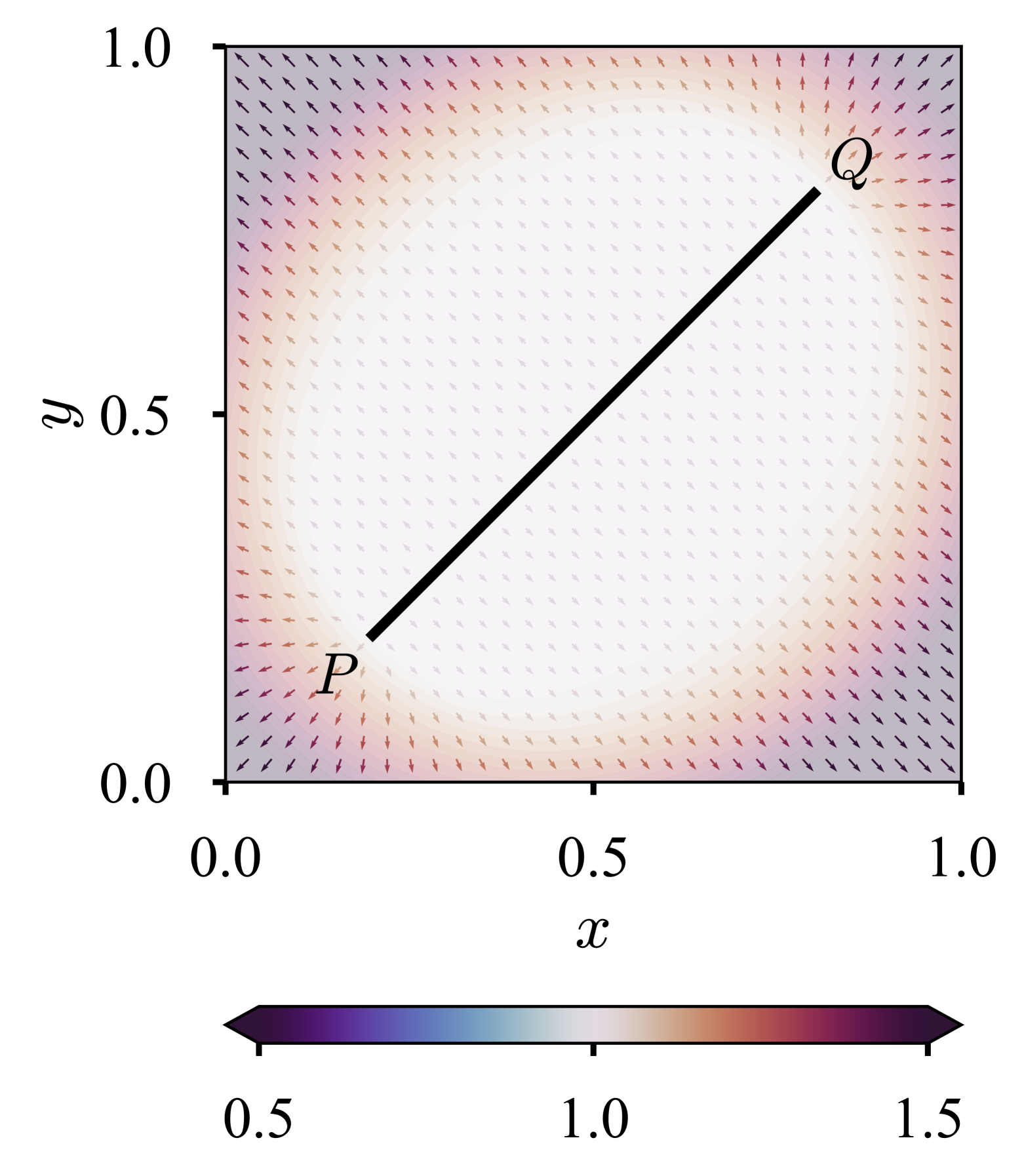
(d) Gradient, $\nabla\phi_{PQ}$

Figure 1: Distance to a line segment. Representations of functions defined in Equations (9), (10), (11), and its gradient. The line segment $S_{PQ}$, realized as the intersection of $\mathbb{S}=\left\{\bm{x}\in\mathbb{R}^{2}\mid s_{PQ}\left(\bm{x}\right)=0\right\}$ and $\mathbb{T}=\left\{\bm{x}\in\mathbb{R}^{2}\mid t_{PQ}\left(\bm{x}\right)\geq 0\right\}$, is represented by $\mathbb{P}=\left\{\bm{x}\in\mathbb{R}^{2}\mid\phi_{PQ}\left(\bm{x}\right)=0\right\}$. $\nabla\phi_{PQ}$ offers the unit normal vector in the vicinity of $S_{PQ}$.

We begin by considering the distance function to a line segment. Let $P\left(=\bm{x}_{P}\right)$ and $Q\left(=\bm{x}_{Q}\right)$ be the endpoints of the line segment $S_{PQ}$, with $S^{\prime}_{PQ}$ denoting the infinite line passing through $P$ and $Q$. First, we define the following signed distance function (SDF) $s_{PQ}$:

$$s_{PQ}\left(\bm{x}\right)=\frac{1}{\|\bm{x}_{PQ}\|}s^{\prime}_{PQ}=\frac{1}{\|\bm{x}_{PQ}\|}\bm{n}_{PQ}\cdot(\bm{x}-\bm{x}_{P}),$$ (9)

where $\|\cdot\|$ denotes the $L^{2}$-norm, $s^{\prime}_{PQ}$ is the signed distance to the infinite line $S^{\prime}_{PQ}$, $\bm{x}_{PQ}=\bm{x}_{Q}-\bm{x}_{P}$ is the vector from $P$ to $Q$, and $\bm{n}_{PQ}$ is the unit normal to $S^{\prime}_{PQ}$. The function $s_{PQ}$ can be viewed as the signed distance function to the infinite line $S^{\prime}_{PQ}$, normalized by the length of the segment of interest, $S_{PQ}$. With these definitions, the line segment $S_{PQ}$ is realized as a subset of $\mathbb{S}=\left\{\bm{x}\in\mathbb{R}^{d}\mid s_{PQ}\left(\bm{x}\right)=0\right\}$. Next, we introduce the trimming function (TF) $t_{PQ}$:

$$t_{PQ}(\bm{x})=\frac{1}{\|\bm{x}_{PQ}\|}\left(\left(\frac{\|\bm{x}_{PQ}\|}{2}\right)^{2}-\|\bm{x}-\bm{x}_{M}\|\right),$$ (10)

where $\bm{x}_{M}=(\bm{x}_{P}+\bm{x}_{Q})/2$ is the midpoint of $S_{PQ}$. The region $\mathbb{T}=\left\{\bm{x}\in\mathbb{R}^{d}\mid t_{PQ}\left(\bm{x}\right)\geq 0\right\}$ corresponds to the circular disk whose radius is $\|\bm{x}_{PQ}\|/2$ and center is $\bm{x}_{M}$. Finally, interpreting the line segment $S_{PQ}$ as the intersection of $\mathbb{S}$ and $\mathbb{T}$, we define the sufficiently smooth approximate distance function (ADF) to the line segment $S_{PQ}$ as follows [50]:

$$\phi_{PQ}(\bm{x})=\left(s_{PQ}^{2}+\left(\frac{\left(s_{PQ}^{4}+t_{PQ}^{2}\right)^{1/2}-t_{PQ}}{2}\right)^{2}\right)^{1/2}.$$ (11)

Figure 1 illustrates the signed distance function $s_{PQ}$, the trimming function $t_{PQ}$, the approximate distance function $\phi_{PQ}$ to the line segment $S_{PQ}$, and its gradient $\nabla\phi_{PQ}$. The segment $S_{PQ}$ lies in the region where both $s_{PQ}=0$ and $t_{PQ}\geq 0$ hold, and is implicitly represented by $\phi_{PQ}=0$. Moreover, $\nabla\phi_{PQ}$ serves as the unit normal vector in the vicinity of $S_{PQ}$, which is beneficial for considering Neumann boundary conditions.

2.2.2 Distance to a domain

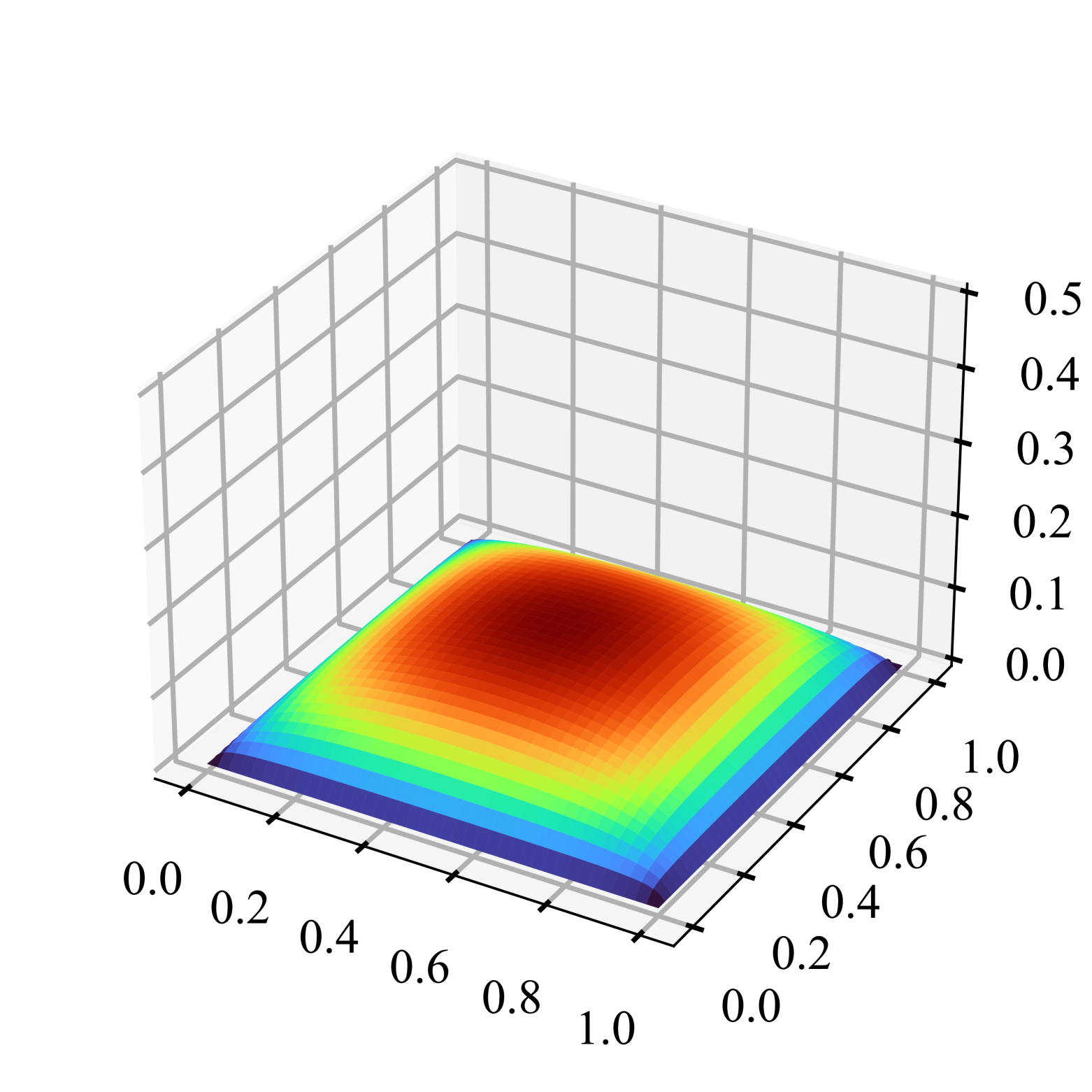
(a) ADF, $\phi^{(1)}$

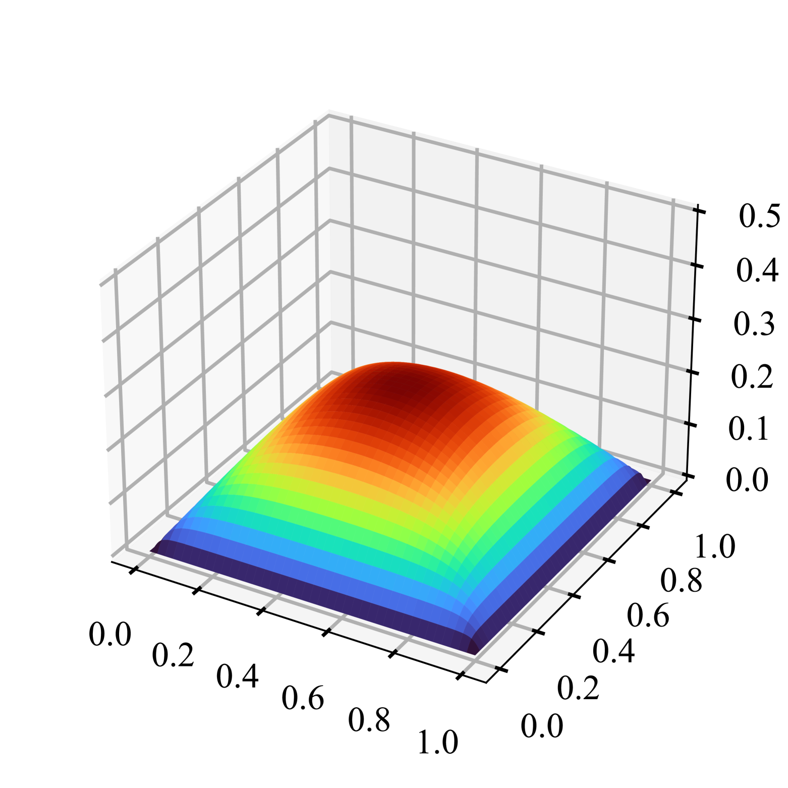
(b) ADF, $\phi^{(2)}$

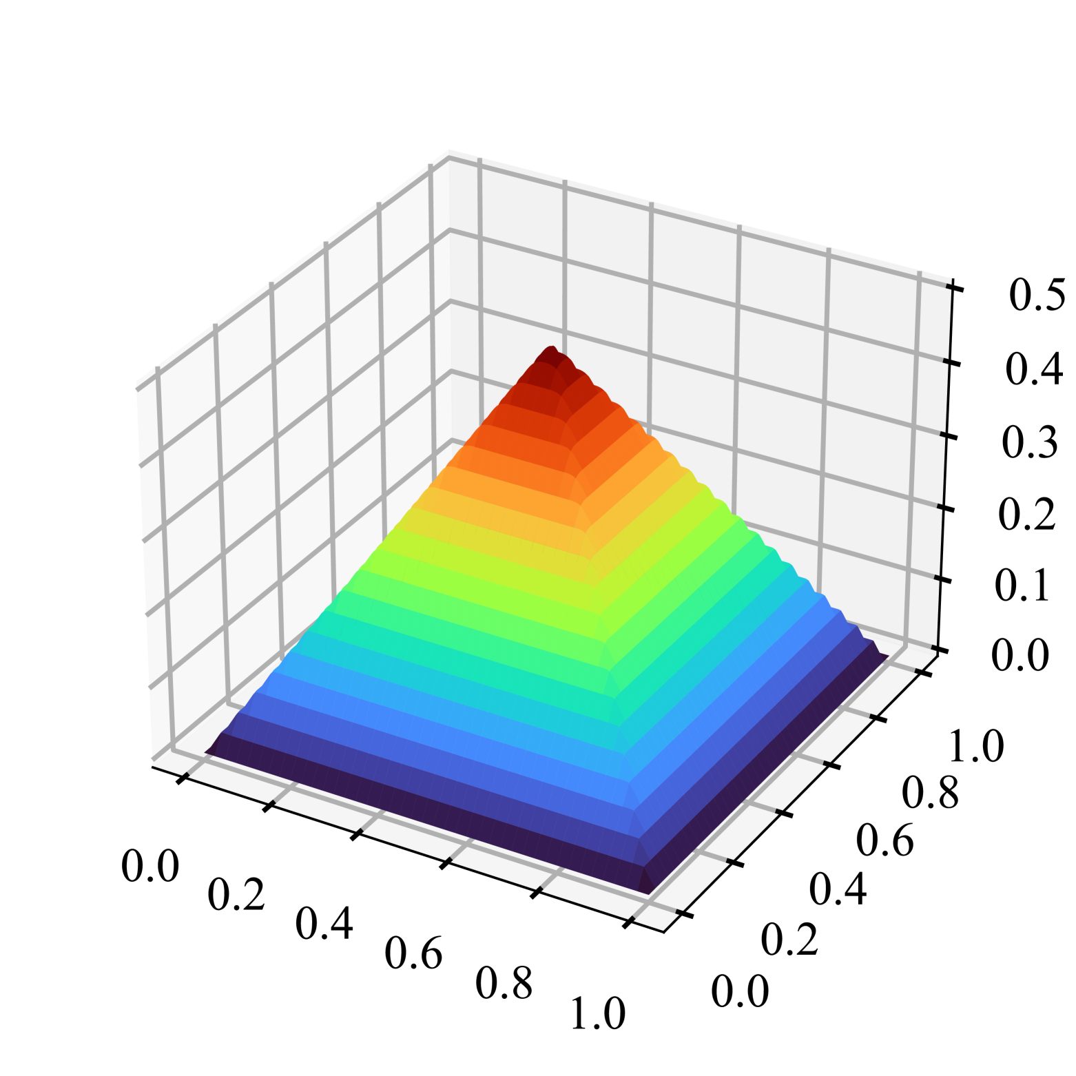
(c) ADF, $\phi^{(64)}$

(d) EDF, $\Phi$

Figure 2: Distance to a domain: square. Normalized ADFs are smooth approximations of the EDF, and approach the EDF as the normalization order is increased.

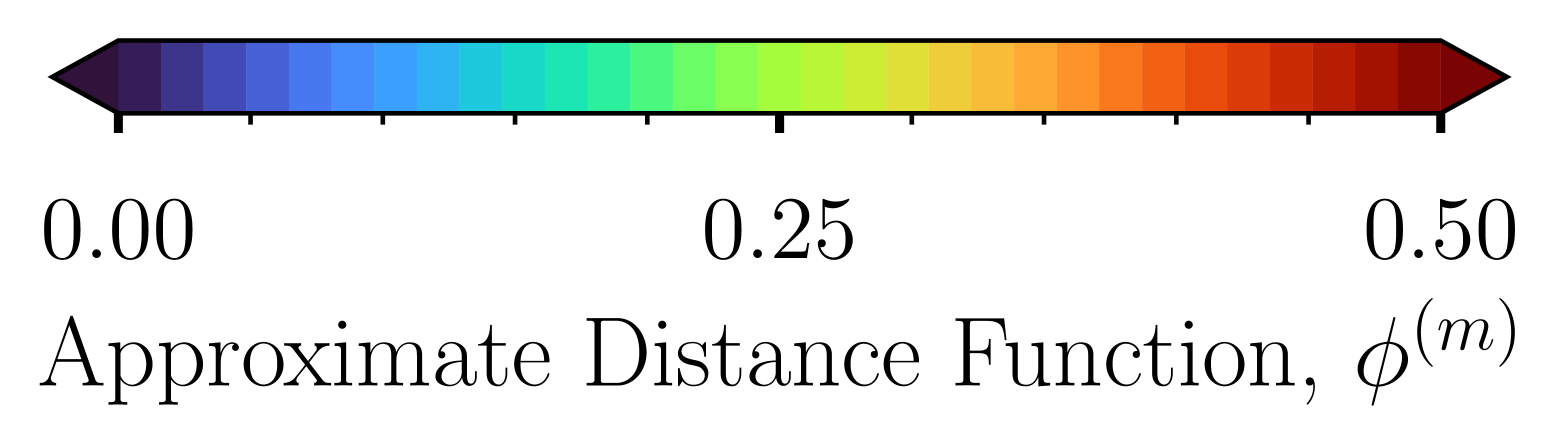
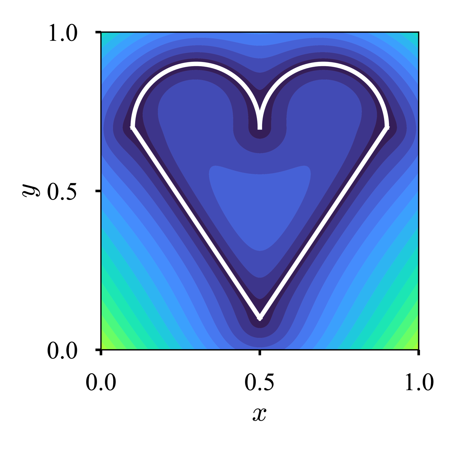
(a) $m=1$

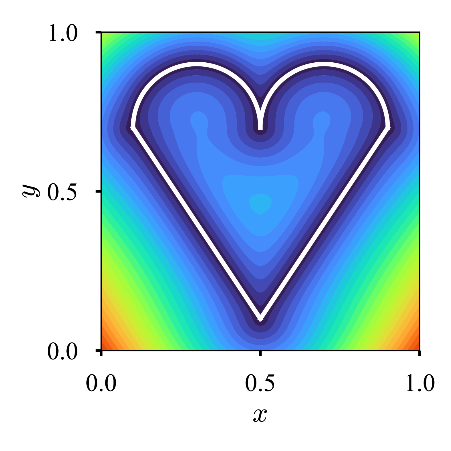
(b) $m=2$

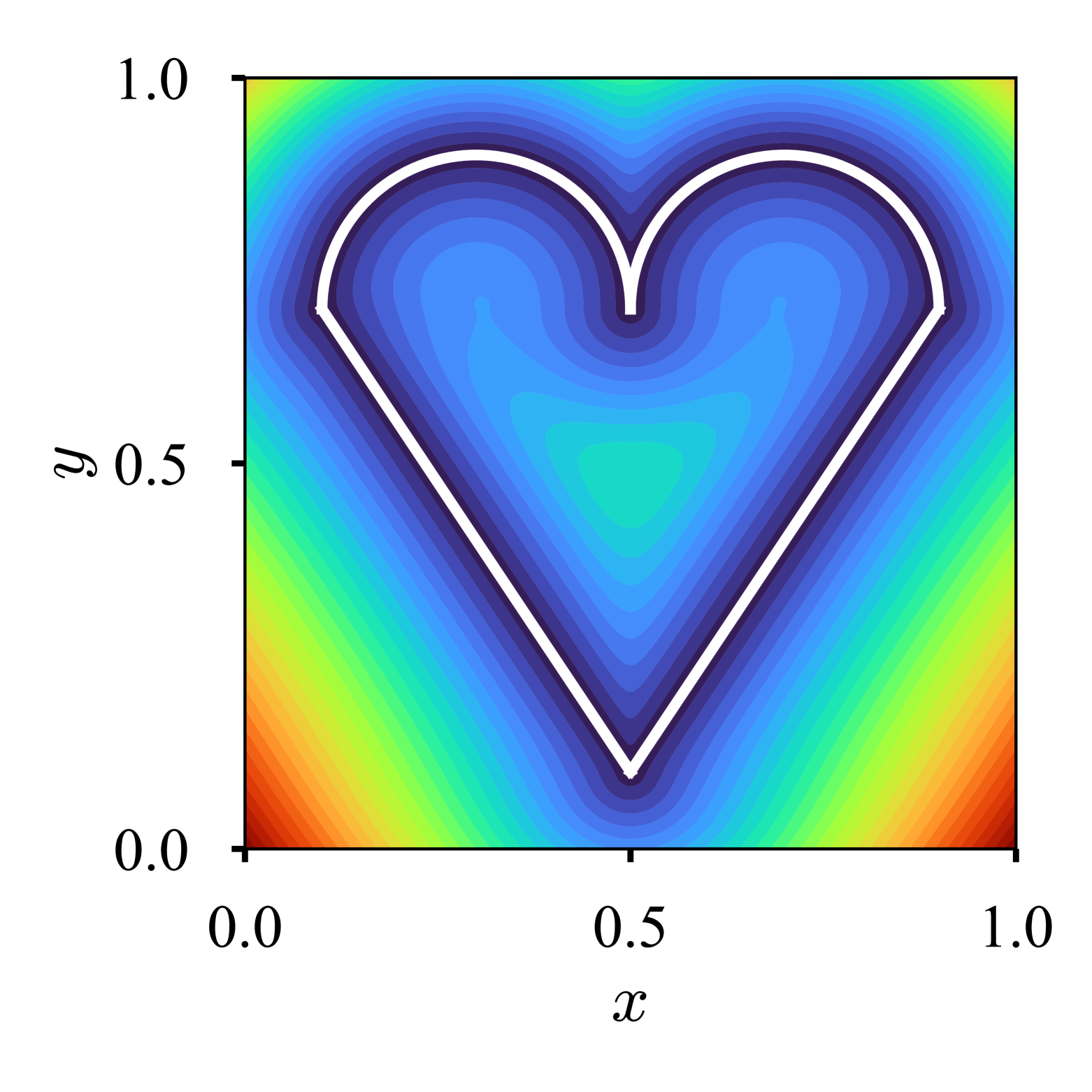
(c) $m=4$

(d) $m=8$

Figure 3: Distance to a domain: heart. Distance to each segment is defined as in Equation (11), then the ADF is constructed by the joining operation as in Equation (12). The ADFs are normalized to the 1st, 2nd, 4th, and 8th orders.

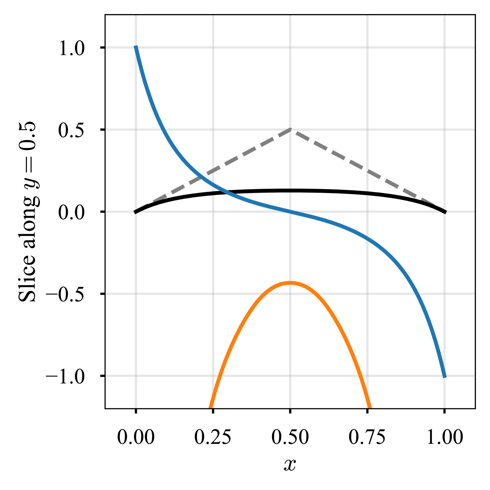
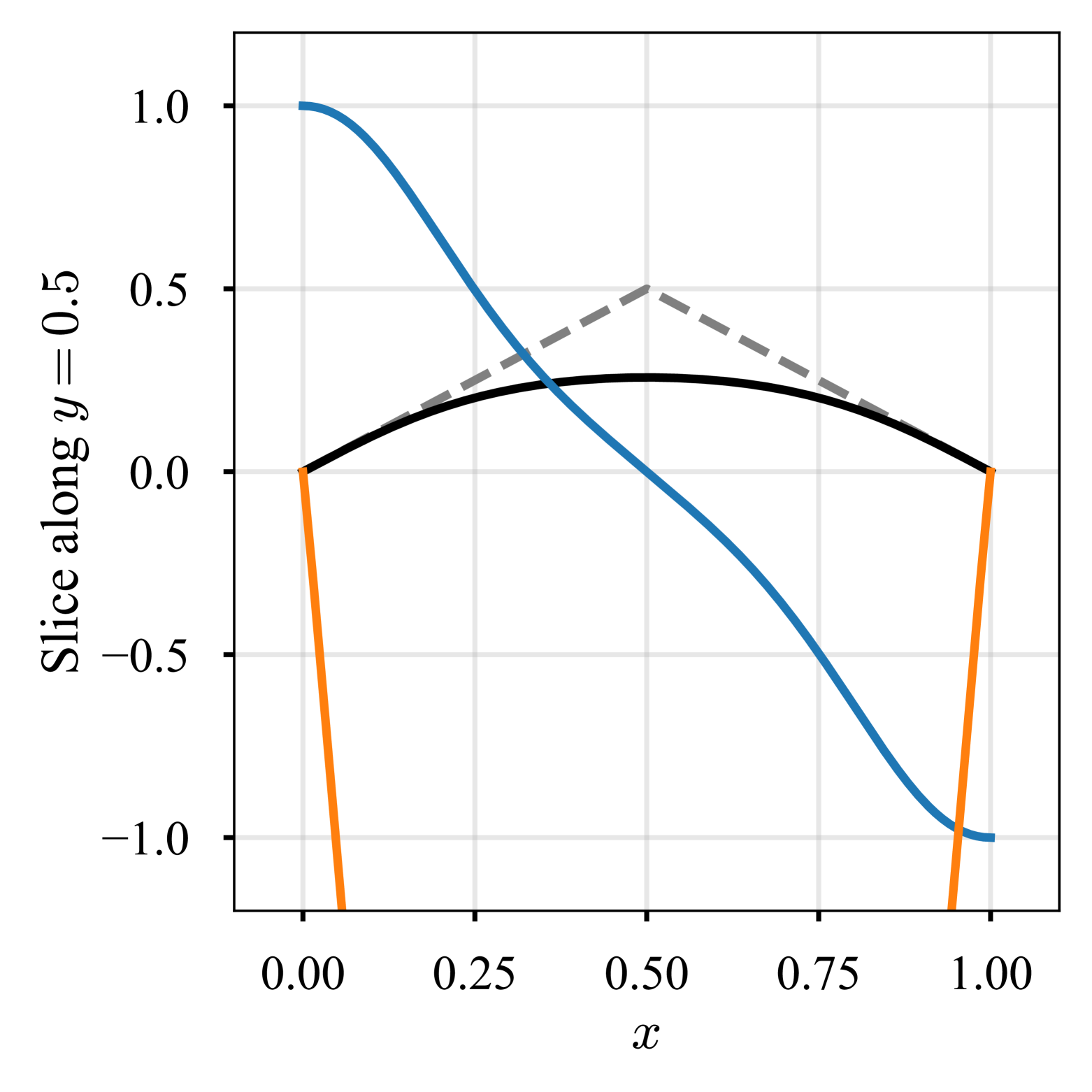
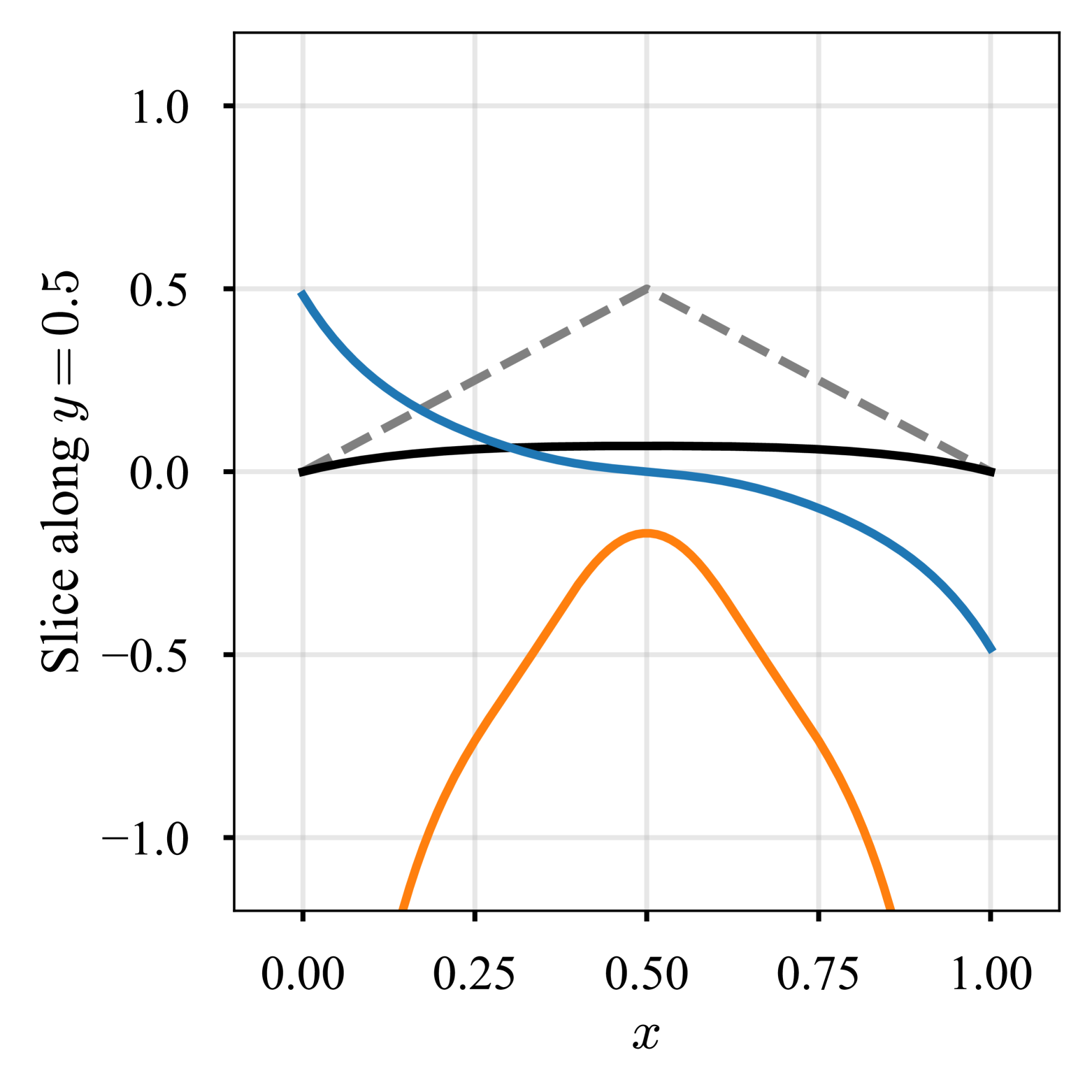
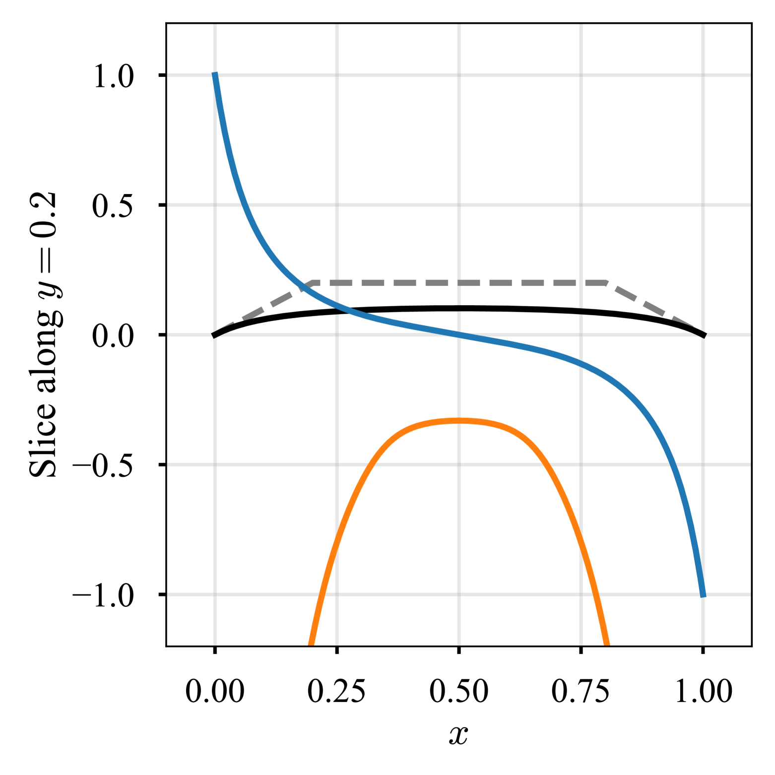
(a) Normalized, $\phi^{(1)}$

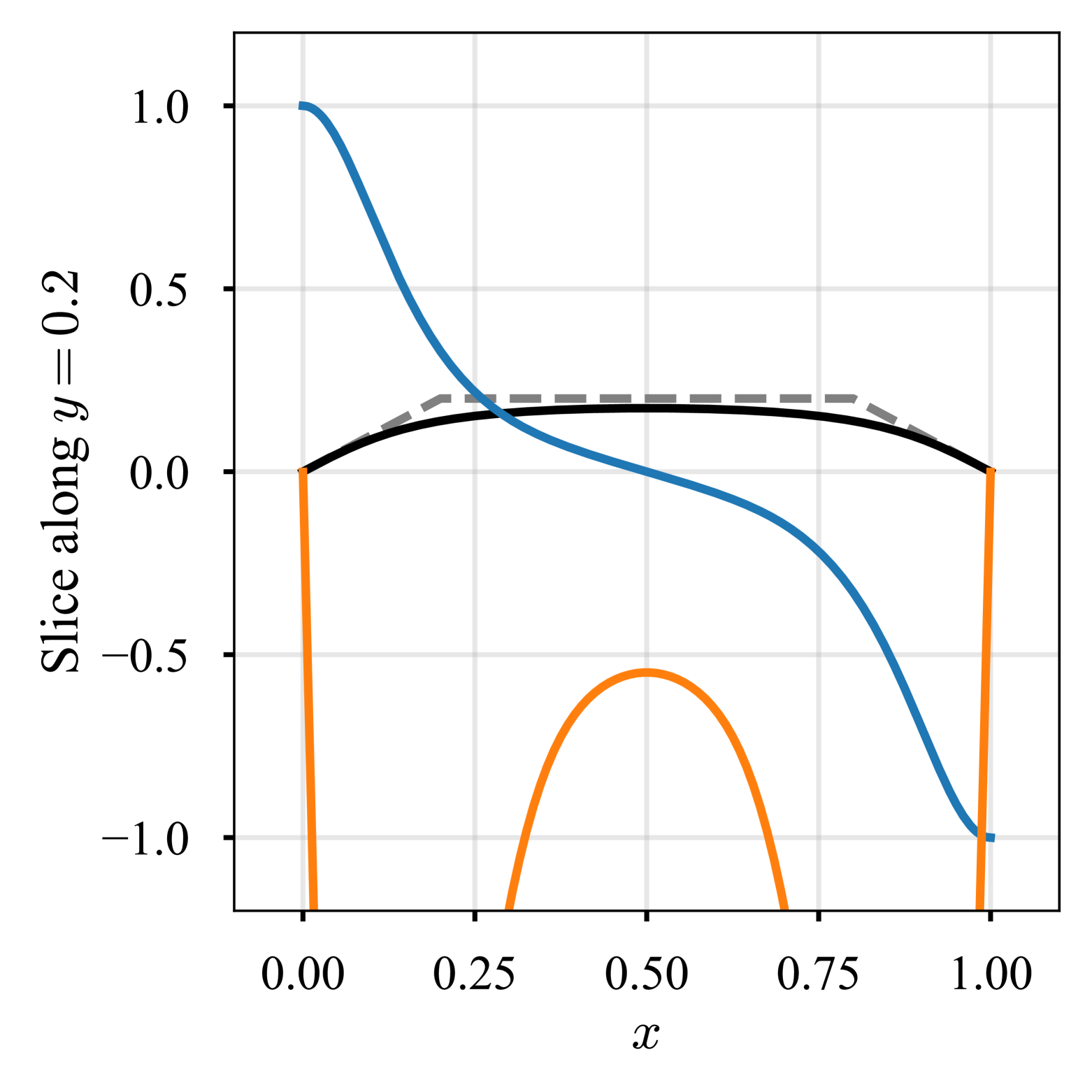
(b) Normalized, $\phi^{(2)}$

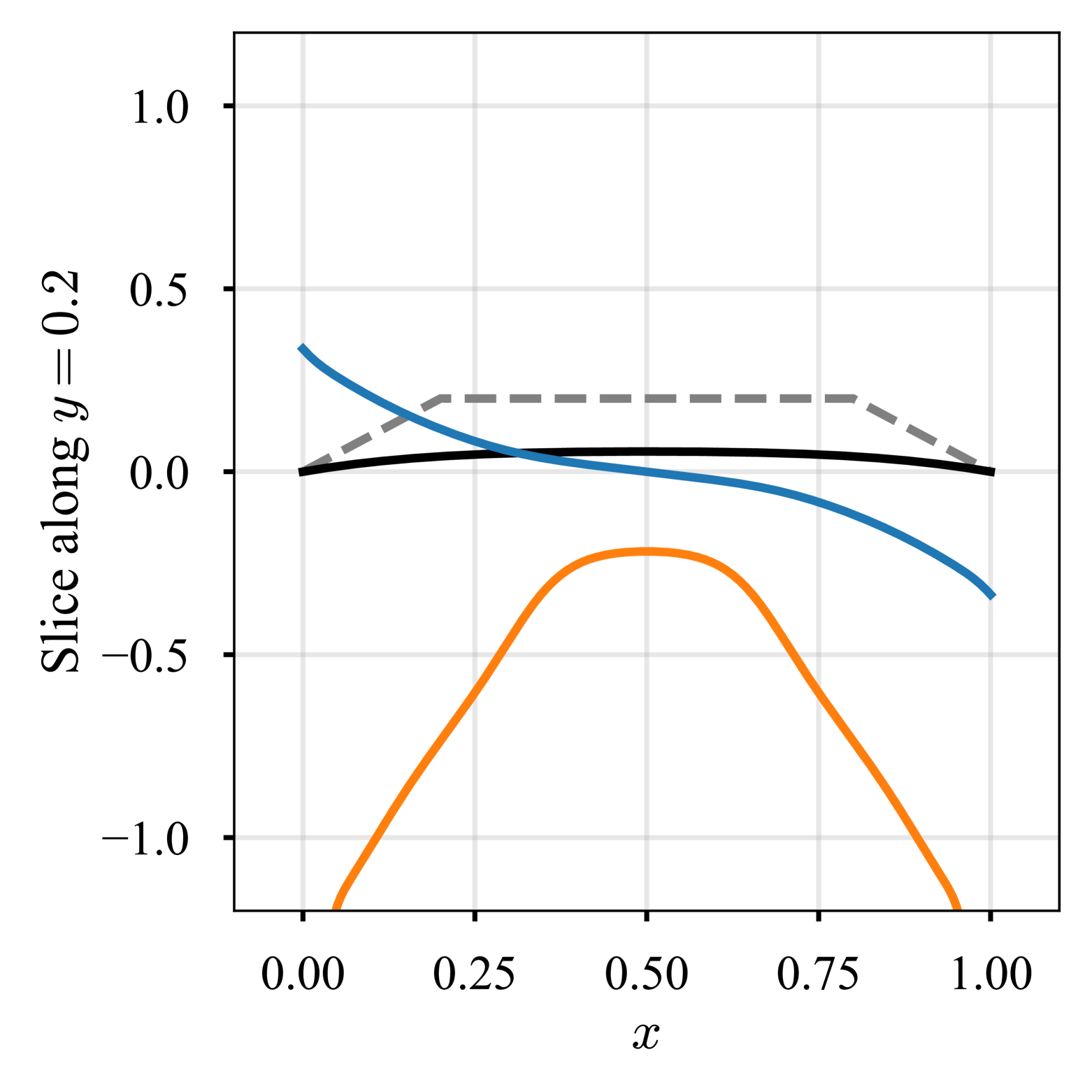
(c) Not normalized, $\varphi$

Figure 4: Distance to a domain: square (slice). (Top) slice along $y=0.5$. (Bottom) slice along $y=0.2$. The 1st derivative of the normalized ADFs form the inward unit normal at the boundary (property (b)), while the 1st derivative of the non-normalized ADF does not (right column). It should be noted that simply multiplying the non-normalized ADF by a constant does not help to satisfy property (b).

Assuming that the boundary $\Gamma$ is composed of piecewise segments ($\Gamma=\bigcup_{i=1}^{N}\Gamma_{i}$), the ADF to $\Gamma$ is constructed via the following joining operation [64, 57]:

$$\phi^{(m)}\coloneq\frac{\prod_{i}\phi_{i}}{\left(\sum_{i}\phi_{i}^{m}\right)^{1/m}}=\frac{1}{\left(\sum_{i}\phi_{i}^{-m}\right)^{1/m}},$$ (12)

where $\phi_{i}$ is the ADF to $\Gamma_{i}$ ($\phi_{i}=0$ on $\Gamma_{i}$) and $m\left(\in\mathbb{Z}_{>0}\right)$ is the normalization order associated with the property (c). Equation (12) is formally known as the R-equivalence operation. While another joining, the R-conjunction operation, is also available, we employ the R-equivalence operation in this study due to its associative property, which the R-conjunction operation lacks. Figure 2 shows the ADFs with different normalization orders and the EDF to a unit square. As depicted, the ADFs serve as smooth approximations of the EDF. The ADFs $\phi^{(m)}$ approach the EDF $\Phi$ as the normalization order $m$ increases, as described in [64]. This is further confirmed by comparing $\phi^{(64)}$ and $\Phi$ in Figure 2. It should be noted that the ADF obtained by Equation (12) generalizes to curves, complex geometries (e.g., Figure 3), and higher-dimensional field [46, 64, 52, 65, 55, 56].

The choice of the normalization order $m$ in Equation (12) is arbitrary, and $m=2$ is commonly used in computational mechanics practice [57]. Our preliminary numerical experiments using $m=1,2,4,8$ found that $m=1$ and $m=2$ achieve similar accuracy and convergence, while $m=4$ and $m=8$ can degrade the convergence speed (see Appendix B). Reflecting this observation and the previous studies [46, 58], we use $m=1$ for the remainder of this study.

As a simpler joining operation, one may consider the following ADF:

$$\varphi\coloneq\prod_{i}\phi_{i}.$$ (13)

Although Equation (13) is known to be another class of R-equivalence operations, and $\varphi$ is easy to construct and satisfies property (a) ($\varphi=0$ on $\Gamma$), it fails to meet property (b) ($\partial_{\bm{\nu}}\varphi\neq 1$ on $\Gamma$). Consequently, $\varphi$ is said to be not normalized [64]. As evidence, Figure 4 presents the ADFs and their 1st and 2nd derivatives at the slices along $y=0.5$ and $y=0.2$. It is clear that $\phi^{(1)}$ and $\phi^{(2)}$ satisfy properties (a) and (b), while $\varphi$ does not.

In this study, we employ Equation (12) to define the ADFs and the unit normal vector on the boundary instead of Equation (13), in order to address mixed boundary value problems. While distance functions in the form of $\varphi$ have been used in several studies  [39, 45, 34, 66], their applicability to complex geometries and mixed boundary value problems, where homogeneous/inhomogeneous Dirichlet, Neumann, Robin, and their combinations are prescribed, is severely limited. Specifically, methods like those in [39, 66] enforce the Dirichlet condition in a hard manner, while relying on a penalty approach for the Neumann boundary condition. This limitation arises from the difficulty in precisely defining the unit normal, which is crucial for the Neumann and mixed problems. In addition, the methods presented therein are constrained to problems defined on convex hulls, and cannot be extended to form distance functions to non-convex geometries, such as shown in Figure 3 and discussed in Section 3.

2.2.3 Approximate solution structure

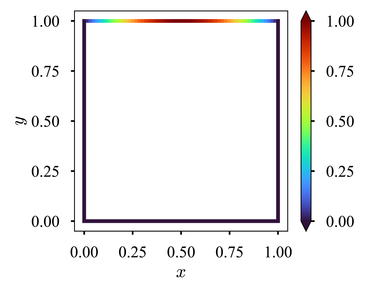
(a) Dirichlet condition, $g_{D}:\Gamma_{D}\to\mathbb{R}$

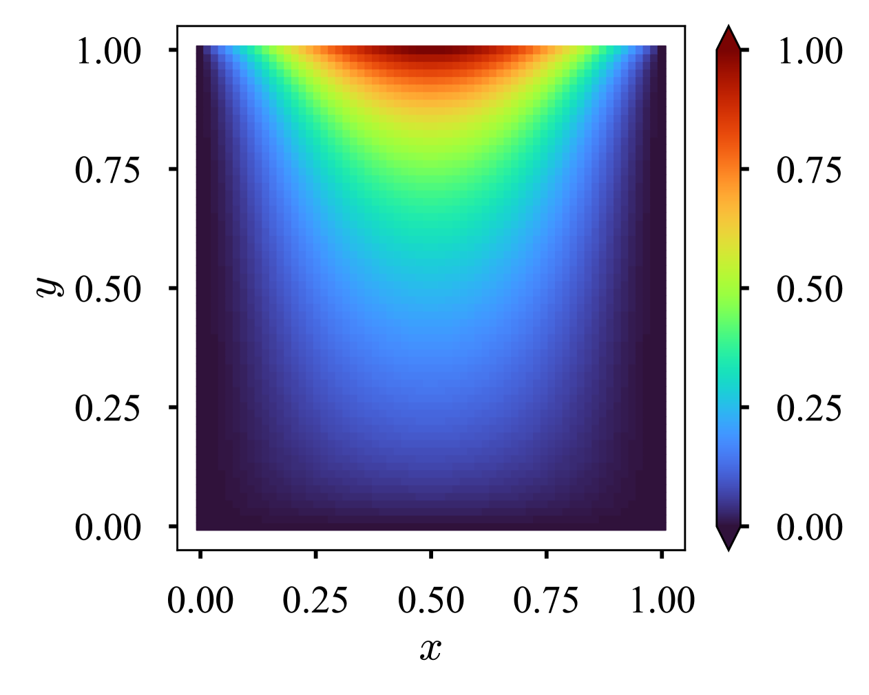
(b) Interpolant, $\bar{g}_{D}:\bar{\Omega}\to\mathbb{R}$

Figure 5: Transfinite interpolation of Dirichlet boundary condition. With the ADF $\phi$ vanishing on the boundary, the trial function $\tilde{u}=\bar{g}_{D}+\phi\hat{u}$ exactly satisfies the Dirichlet boundary condition, $g_{D}$.

For simplicity, we only discuss the treatment of Dirichlet boundary condition. However, the method can be extended to Neumann, Robin, and mixed boundary conditions, as described in [46, 55, 56, 67] and demonstrated in Section 3.

As mentioned in Section 1, boundary conditions can be imposed in either soft [9] or hard manner [2, 39, 46], in the context of PINN. In the soft imposition approach, the raw output of the neural network serves as the approximate solution:

$$u\simeq\mathcal{I}\left(\hat{u}\right)\coloneqq\hat{u},$$ (14)

where $\mathcal{I}\left(\cdot\right)$ is the identity operator. Since no explicit treatment is applied and the neural network $\hat{u}$ is not constrained, boundary conditions are enforced through the additional penalty terms in the loss function.

In contrast, the hard imposition approach directly enforces the boundary condition by constructing the approximate solution through the following projection:

$$u\simeq\mathcal{P}\left(\hat{u}\right)\coloneqq\tilde{u}\coloneqq\bar{g}_{D}+\phi_{D}\hat{u},$$ (15)

where $\bar{g}_{D}$ is an interpolation of the Dirichlet condition ($\bar{g}_{D}=g_{D}$ on $\Gamma_{D}$), and $\phi_{D}$ is the approximate distance function (ADF) to $\Gamma_{D}$. With $\phi_{D}$ vanishing on $\Gamma_{D}$, $\tilde{u}$ readily satisfies the imposed Dirichlet boundary condition. When the Dirichlet boundary $\Gamma_{D}$ consists of multiple segments $\Gamma_{i}$ ($i=1,\ldots,N_{D}$) (i.e., Dirichlet conditions are prescribed on multiple segments), the interpolant $\bar{g}_{D}$ can be constructed by transfinite interpolation [51]:

$$\bar{g}_{D} =\sum_{i}w_{i}g_{i},$$ (16)

$$w_{i} =\frac{\phi_{i}^{-\mu_{i}}}{\sum_{j}\phi_{j}^{-\mu_{j}}}=\frac{\prod_{j;j\neq i}\phi_{j}^{\mu_{j}}}{\sum_{k}\prod_{j;j\neq k}\phi_{j}^{\mu_{j}}},$$ (17)

where $g_{i}$ is the Dirichlet BC prescribed on $\Gamma_{i}$, $\mu_{i}$ is the interpolation order ($\bar{g}_{D}$ is $(\mu_{i}-1)$-times continuously differentiable on $\Gamma_{i}$), and $w_{i}$ forms a partition of unity.

For example, given the Dirichlet conditions:

$$g_{1} =0 \quad\text{on}\quad\Gamma_{1}=\{(x,0)\mid x\in(0,1)\},$$ (18)

$$g_{2} =0 \quad\text{on}\quad\Gamma_{2}=\{(1,y)\mid y\in(0,1)\},$$ (19)

$$g_{3} =\sin(\pi x) \quad\text{on}\quad\Gamma_{3}=\{(x,1)\mid x\in(0,1)\},$$ (20)

$$g_{4} =0 \quad\text{on}\quad\Gamma_{4}=\{(0,y)\mid y\in(0,1)\},$$ (21)

the corresponding interpolant is shown in Figure 5, demonstrating how $g_{D}$ is smoothly extended to $\bar{g}_{D}$. Notably, the projection in Equation (15) restricts the admissible solution space, ensuring that the trial function is selected from $U=\{u:\Omega\to\mathbb{R}\mid u=g_{D}\text{ on }\Gamma_{D}\}$ which is analogous to the approach used in classical numerical methods such as the Galerkin method. This direct enforcement of boundary conditions allows for improved accuracy and stability compared to the penalty-based soft imposition approach.

2.3 Adaptive weight tuning for gradient imbalance

The formulation described in Section 2.2 ensures that the approximate solution inherently satisfies the prescribed boundary conditions. Consequently, $\mathcal{L}_{\text{BC}}$ in Equation (5) becomes identically zero. This implies that, for forward problems, minimizing $\mathcal{L}_{\text{PDE}}$ alone is sufficient, akin to classical numerical methods. However, in inverse problems, PINN must incorporate observed data through Equation (8). In this case, the loss function with hard boundary condition enforcement takes the form:

$$\mathcal{L}(\bm{\theta})=\tilde{\mathcal{L}}_{\text{PDE}}(\bm{\theta})+\lambda_{\text{Data}}\tilde{\mathcal{L}}_{\text{Data}}(\bm{\theta}),$$ (22)

where $\tilde{\mathcal{L}}_{\text{PDE}}$ and $\tilde{\mathcal{L}}_{\text{Data}}$ are the modified PDE and data loss functions, respectively, obtained by replacing $\hat{u}$ with $\tilde{u}$ in Equations (6) and (8).

A critical challenge in optimizing multi-objective functions, such as Equation (22), is the risk of convergence to undesired, suboptimal Pareto solutions due to gradient imbalance, which can further lead to the emergence of trivial, constant solutions, known as failure modes [68, 63, 47, 69]. In such cases, appropriate normalization is crucial to balance the gradients of multiple loss terms. In the context of PINN, the PDE and data loss terms are typically of different magnitudes, and their gradients may not be directly comparable. To address this issue, we employ an adaptive weight tuning method known as dynamic normalization [47]. This method adaptively adjusts the weight $\lambda_{\text{Data}}$ in Equation (22) to balance the gradients of each loss term during the process of optimization, eliminating the need for manual tuning.

We first consider the first-order Taylor series expansion of the loss function around the current parameter $\bm{\theta}^{(n)}$:

$$\mathcal{L}(\bm{\theta}^{(n)}+\Delta\bm{\theta})-\mathcal{L}(\bm{\theta}^{(n)})=\Delta\bm{\theta}^{\top}\nabla_{\bm{\theta}}\mathcal{L}(\bm{\theta}^{(n)}),$$ (23)

where $\Delta\bm{\theta}=\bm{\theta}^{(n+1)}-\bm{\theta}^{(n)}$ represents the update. In gradient descent, the update is given by:

$$\begin{split}\Delta\bm{\theta}&=\bm{\theta}^{(n+1)}-\bm{\theta}^{(n)}\\ &=-\eta^{(n)}\nabla_{\bm{\theta}}\mathcal{L}(\bm{\theta}^{(n)}),\end{split}$$ (24)

where $\eta^{(n)}$ is the learning rate. Substituting this into Equation (23) yields:

$$\Delta\tilde{\mathcal{L}}_{\text{PDE}}+\Delta\tilde{\mathcal{L}}_{\text{Data}}=-\eta^{(n)}\|\nabla_{\bm{\theta}}\tilde{\mathcal{L}}_{\text{PDE}}+\lambda_{\text{Data}}\nabla_{\bm{\theta}}\tilde{\mathcal{L}}_{\text{Data}}\|^{2}.$$ (25)

Here, $\Delta\tilde{\mathcal{L}}_{\text{PDE}}$ and $\Delta\tilde{\mathcal{L}}_{\text{Data}}$ denote the changes in the PDE and data loss terms, respectively. For simplicity, we assume that each gradient is orthogonal to the other. While this assumption may not always hold, it greatly simplifies the scope, and the resultant adaptive weights have been shown to provide significant performance improvements in practice  [30, 24, 70, 47, 71]. If the orthogonality assumption poses a severe issue, projection techniques such as those presented in [72] can be employed to mitigate conflicts by projecting backpropagated gradients onto orthogonal directions. Under the aforementioned orthogonality assumption, we split Equation (25) into:

$$\Delta\tilde{\mathcal{L}}_{\text{PDE}} =-\eta^{(n)}\|\nabla_{\bm{\theta}}\tilde{\mathcal{L}}_{\text{PDE}}\|^{2},$$ (26)

$$\Delta\tilde{\mathcal{L}}_{\text{Data}} =-\eta^{(n)}\lambda_{\text{Data}}^{2}\|\nabla_{\bm{\theta}}\tilde{\mathcal{L}}_{\text{Data}}\|^{2}.$$ (27)

Based on the analysis in [30, 63], it is desirable to balance the reduction of the PDE and data loss such that they are reduced at similar rates, $\Delta\tilde{\mathcal{L}}_{\text{PDE}}\sim\Delta\tilde{\mathcal{L}}_{\text{Data}}$. This translates to the following adaptive weight tuning strategy:

$$\lambda_{\text{Data}}^{(n)}=\frac{\|\nabla_{\bm{\theta}}\tilde{\mathcal{L}}_{\text{PDE}}\|}{\|\nabla_{\bm{\theta}}\tilde{\mathcal{L}}_{\text{Data}}\|}.$$ (28)

In practice, the exponential decay is applied to stabilize the fluctuations  [24, 30, 31]:

$$\hat{\lambda}_{\text{Data}}^{(n)}=\beta\hat{\lambda}_{\text{Data}}^{(n-1)}+(1-\beta)\lambda_{\text{Data}}^{(n)},$$ (29)

where $\beta\in[0,1)$ is the decay rate. Our preliminary numerical experiments indicate that $\beta$ should be set to a value close to 1 to ensure stability. However, as is well known, setting $\beta$ too close to 1 can lead to slow convergence. As an illustration, applying Equation (29) repeatedly, one obtains:

$$\hat{\lambda}_{\text{Data}}^{(n)} =\beta^{n}\hat{\lambda}_{\text{Data}}^{(0)}+(1-\beta)\sum_{k=1}^{n}\beta^{n-k}\lambda_{\text{Data}}^{(k)},$$ (30)

$$\begin{split}\therefore\mathbb{E}\left[\hat{\lambda}_{\text{Data}}^{(n)}\right]&=\beta^{n}\hat{\lambda}_{\text{Data}}^{(0)}+(1-\beta)\sum_{k=1}^{n}\beta^{n-k}\mathbb{E}\left[\lambda_{\text{Data}}^{(k)}\right]\\ &=\beta^{n}\hat{\lambda}_{\text{Data}}^{(0)}+\mathbb{E}\left[\lambda_{\text{Data}}^{(n)}\right](1-\beta)\sum_{k=1}^{n}\beta^{n-k}\\ &=\beta^{n}\hat{\lambda}_{\text{Data}}^{(0)}+\mathbb{E}\left[\lambda_{\text{Data}}^{(n)}\right](1-\beta^{n}).\end{split}$$ (31)

One can instantly realize that $\hat{\lambda}_{\text{Data}}^{(n)}$ is biased towards its initial value $\hat{\lambda}_{\text{Data}}^{(0)}$, particularly when $\beta$ is close to 1 and $n$ is not sufficiently large. To remove this initialization bias, we set $\hat{\lambda}_{\text{Data}}^{(0)}=0$ and introduce bias correction as in [73]:

$$\tilde{\lambda}_{\text{Data}}^{(n)}=\frac{\hat{\lambda}_{\text{Data}}^{(n)}}{1-\beta^{n}},$$ (32)

ergo $\mathbb{E}[\tilde{\lambda}_{\text{Data}}^{(n)}]=\mathbb{E}[\lambda_{\text{Data}}^{(n)}]$, whereas $\mathbb{E}[\hat{\lambda}_{\text{Data}}^{(n)}]\neq\mathbb{E}[\lambda_{\text{Data}}^{(n)}]$. Equation (32) ensures that the weight is properly adjusted, even in the early stages of optimization and when $\beta$ is near 1. Despite the presence of numerous studies on adaptive weight tuning in the context of PINN  [30, 24, 70, 31], discussion on this initialization bias is often overlooked. Bias correction technique in Equation (32) is crucial for the appropriate adjustment, ensuring $\Delta\tilde{\mathcal{L}}_{\text{PDE}}\sim\Delta\tilde{\mathcal{L}}_{\text{Data}}$ is satisfied from the initial stage. The effectiveness of bias-corrected dynamic normalization has already been demonstrated in [47, 74] for both forward and inverse problems, and is further confirmed in Section 3.

2.4 Positivity enforcement for inverse analysis

When applied to inverse problems, PINNs are typically equipped with additional trainable parameters to represent the physical quantities of interest. For instance, when identifying the diffusion coefficient $\kappa$ in a diffusion equation, an additional parameter $\hat{\kappa}$ is introduced to represent and estimate $\kappa$ from the available observations. This approach has been widely used in the literature, as exemplified in [9, 14, 75, 76]. Since $\hat{\kappa}$ is a trainable parameter, it is updated alongside the network parameters (weights and biases). This allows $\hat{\kappa}$ to take any real value, including negative values. Such an approach can be viewed as a class of soft imposition, as the sign of $\hat{\kappa}$ is not explicitly constrained and is only expected to be learned through the optimization process. From a physical point of view, however, these quantities must possess specific signs to ensure physical validity. In the case of diffusion example, the diffusion coefficient $\kappa$ must remain positive.

We address this issue by enforcing the positivity of the physical quantities through the following transformation:

$$\kappa\simeq\tilde{\kappa}\coloneqq h_{+}(\hat{\kappa}).$$ (33)

Here, $h_{+}(\cdot)$ is a bijective function that maps any real value to a positive real realm ($h_{+}:\mathbb{R}\to\mathbb{R}_{+}$). We refer to this transformation as positivity enforcement. In this study, we utilize the exponential function $\exp(\cdot)$ as $h_{+}(\cdot)$, since it showed superior convergence in the prior experiments, where we compared against softplus and rectified power unit, $\text{RePU}_{p=2}=\max(0,\cdot)^{2}$. It is important to note that this transformation is not limited to scalar parameters but can also be applied to space-dependent physical quantities, ensuring physically meaningful estimations across various applications.

3 Numerical results

This section presents the results of several numerical experiments. Throughout the experiments, we employed MLPs with a depth of 5 and a width of 64, initialized by the Glorot method [77]. This choice is based on prior studies demonstrating its effectiveness across a broad range of problems [39, 70, 63, 78]. The Adam optimizer [73] was used for training, with exponential decay rates of 0.9 and 0.999 for the first and second moment estimates, respectively.

As is well known, the choice of the activation function significantly affects the convergence and stability. Common choices include the hyperbolic tangent function and the rectified linear unit (ReLU, $\max(0,\cdot)$). However, the ReLU and some of its variants [79, 80, 81] are generally unsuitable for PINNs because their higher-order derivatives vanish over a wide range of inputs. This limitation hinders the accurate computation of higher-order derivatives of the solution, leading to inaccurate PDE residual calculations [82]. Several studies have also reported numerical results that the ReLU leads to poor convergence in PINNs [83, 84]. Recent research has proposed the rectified power unit ($\text{RePU}_{p}=\max(0,\cdot)^{p},p\in\mathbb{Z}_{\geq 2}$) as an alternative [46, 12]. However, RePU networks are prone to vanishing gradients for inputs less than 1 and exploding gradients for inputs greater than 1, particularly in deeper networks. Indeed, Sukumar and Srivastava [46] and Samaniego et al. [12] utilized RePU networks with a depth of 3, which is relatively shallow in the literature. Our preliminary experiments also confirmed that the RePU network with increased depth (4, 5, and 6) exhibited vanishing and exploding gradient issues, leading to instability. Consequently, we evaluated and compared the hyperbolic tangent, Sigmoid Linear Unit (SiLU) [85, 86], and Gaussian Error Linear Unit (GELU) [87] activation functions. These functions are $C^{\infty}$-continuous and have non-vanishing higher-order derivatives, which are essential for properly calculating the PDE residuals.

Furthermore, several techniques have been proposed to enhance PINN performance, including adaptive activation functions [83, 88, 89], gradient enhancement [25], and self-adaptive soft attention mechanisms [90, 91]. However, based on the authors’ experience, the accuracy improvements achieved by these methods are often marginal and highly sensitive to hyperparameter selection (see Appendix A for numerical results). Hence, we focus on the fundamental aspects of PINN, such as boundary condition treatment and adaptive weight tuning.

We have implemented all the experiments using TensorFlow [92] .

3.1 Forward problem: Poisson equation with mixed boundary conditions

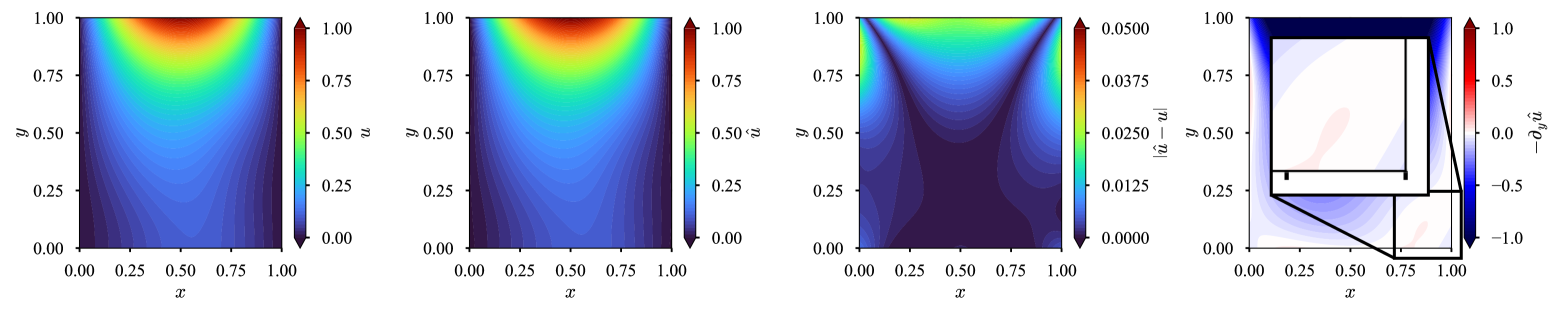
(a) Soft imposition (weight parameter: $\lambda_{\text{BC}}=1$). Relative $L^{2}$ error: $2.88\times 10^{-2}$.

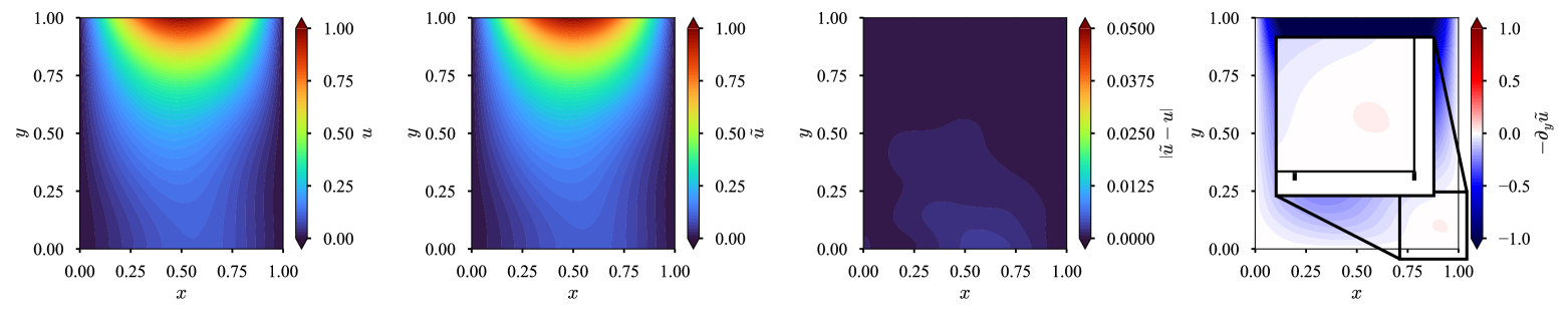
(b) Hard imposition (normalization order: $m=1$). Relative $L^{2}$ error: $3.13\times 10^{-3}$.

Figure 6: Poisson equation with mixed boundary conditions: homogeneous Neumann condition case. (From left to right) Reference solution, approximate solution, absolute error against the reference solution, first derivative of the approximate solution along the negative $y$-axis. Results with GELU activation function. Soft imposition fails to enforce the Dirichlet (third column) and Neumann (fourth column) boundary conditions, while hard imposition successfully enforces both.

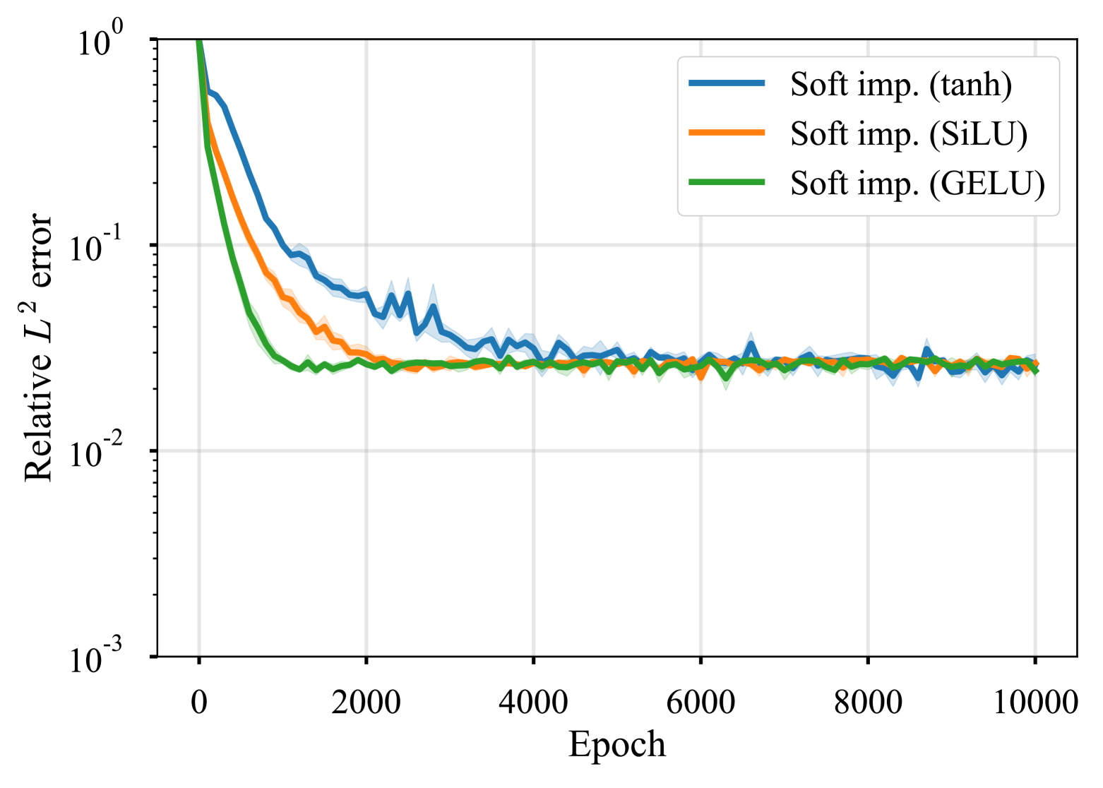
(a) Soft imposition (weight parameter: $\lambda_{\text{BC}}=1$).

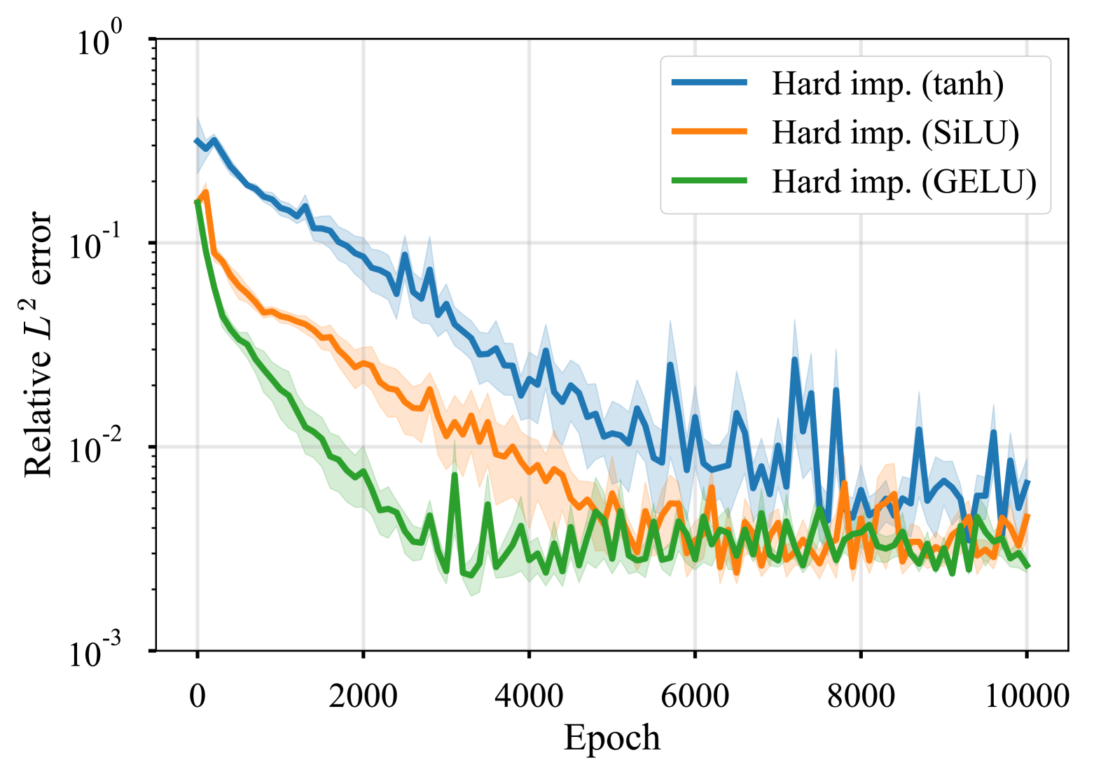
(b) Hard imposition (normalization order: $m=1$).

Figure 7: Poisson equation with mixed boundary conditions: homogeneous Neumann condition case. Relative $L^{2}$ error of the approximate solution with different activation functions. The solid line represents the mean, and the shaded area represents the standard error over 5 independent runs with i.i.d. initialization. Soft imposition quickly plateaus regardless of the activation function.

Table 1: Poisson equation with mixed boundary conditions: homogeneous Neumann condition case. Relative $L^{2}$ error of the approximate solution with different activation functions. Mean and standard error over 5 independent runs with i.i.d. initialization. All values are scaled by $10^{-3}$.

Activation function	Soft imposition	Hard imposition
tanh	$26.26\pm 3.23$	$6.65\pm 2.08$
SiLU	$26.64\pm 0.63$	$4.54\pm 1.05$
GELU	$24.50\pm 1.64$	$2.62\pm 0.21$

Homogeneous Neumann condition case

We first consider the forward problem of the Poisson equation with mixed boundary conditions to assess the effectiveness of soft and hard boundary condition impositions. In addition, we compare the approximation performance of the three aforementioned activation functions: tanh, SiLU, and GELU. The domain is a unit square $\Omega=(0,1)^{2}$, and the boundary is partitioned into Dirichlet and Neumann boundaries: $\Gamma_{D}=\Gamma_{2}\cup\Gamma_{3}\cup\Gamma_{4}$ and $\Gamma_{N}=\Gamma\setminus\Gamma_{D}$ (identical to Equations (18)–(21), except for Equation (18) being replaced by the Neumann boundary). The source and the boundary conditions are set as follows:

$$f =\sin\left(2\pi(x+y)\right),$$ (34)

$$g_{D} =\begin{cases}\sin\left(\pi x\right)&\text{on}\quad\Gamma_{3},\\ 0&\text{on}\quad\Gamma_{2}\cup\Gamma_{4},\end{cases}$$ (35)

$$g_{N} =0.$$ (36)

The reference solution was obtained using the finite difference method (FDM) with a spatial resolution of $\Delta x=\Delta y=5\times 10^{-3}$. Although the FDM solution contains numerical errors, we treat it as the reference as it satisfies the boundary conditions precisely. For both soft and hard boundary condition impositions, the number of collocation points was set to $N_{\text{PDE}}=4,096$. Additionally, $N_{\text{DBC}}=256\times 3$ and $N_{\text{NBC}}=256$ points were added for the soft imposition. The learning rate of the Adam optimizer was set to $10^{-3}$. The weight parameter $\lambda_{\text{BC}}$ in the soft imposition was set to unity, and the normalization order $m$ in the hard imposition was set to 1, based on numerical tests in Appendix B.

Figure 6 presents reference solution, approximate solution, absolute error, and the first derivative of the approximate solution along the negative $y$-direction, so that one can observe how well the Dirichlet and Neumann boundary conditions are satisfied. While a visual comparison of the second column suggests that soft and hard impositions yield similar solutions, the third and fourth columns reveal a significant difference. The soft imposition fails to properly enforce the prescribed Dirichlet and Neumann boundary conditions, whereas the hard imposition does so effectively, as evidenced by the absolute error and derivative plots. The relative $L^{2}$ error further emphasizes the importance of boundary condition treatment. The error of the hard imposition is $3.13\times 10^{-3}$, which is an order of magnitude lower than that of the soft imposition, $2.88\times 10^{-2}$. Figure 7 shows the relative $L^{2}$ error of the approximate solution with different activation functions and boundary condition impositions. We observe from Figure 7 (a) that the soft imposition exhibits a plateau regardless of the activation function, which is known as pitfall of soft boundary condition enforcement [39]. This behavior is likely due to the presence of multiple competing objectives, which makes it difficult for the network to learn the correct solutions [63]. In contrast, the hard imposition demonstrates superior convergence, achieving a relative error of $\mathcal{O}(10^{-3})$ (Figure 7 (b)). Comparing the convergence behavior of different activation functions, we find that both soft and hard impositions converge more rapidly with SiLU and GELU than with tanh. This should be attributed to the non-saturating property of SiLU and GELU, which allows the network to learn more effectively. Moreover, GELU exhibits slightly faster convergence than SiLU, which is likely due to its steeper gradient around the origin. Furthermore, Table 1 summarizes the relative error with different activation functions and boundary condition impositions. One can observe that the hard imposition consistently outperforms the soft imposition across all activation functions, confirming the effectiveness of the hard boundary condition imposition in PINN.

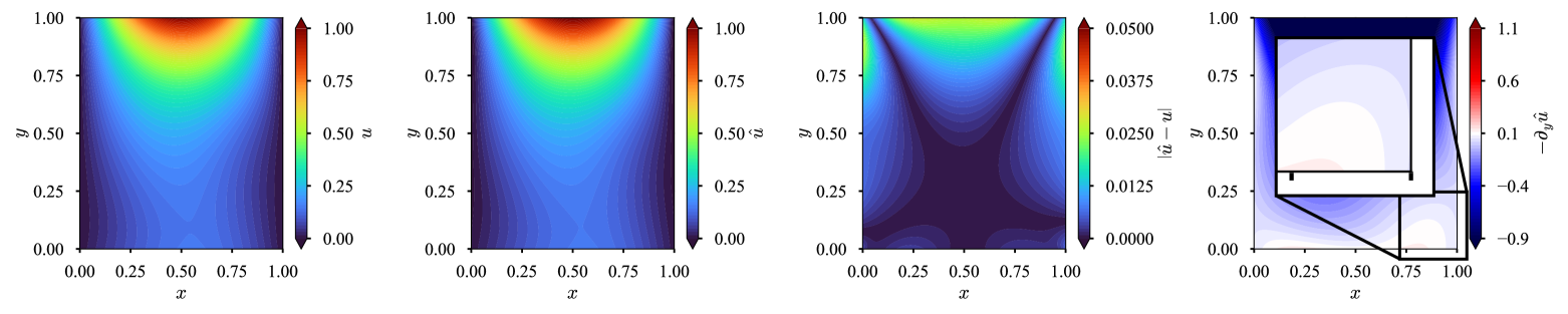
(a) Soft imposition (weight parameter: $\lambda_{\text{BC}}=1$). Relative $L^{2}$ error: $2.87\times 10^{-2}$.

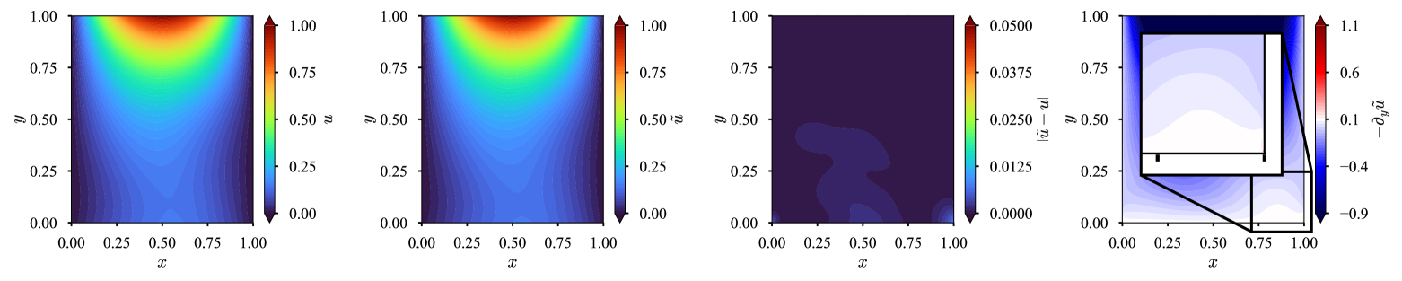
(b) Hard imposition (normalization order: $m=1$). Relative $L^{2}$ error: $2.11\times 10^{-3}$.

Figure 8: Poisson equation with mixed boundary conditions: inhomogeneous Neumann condition case. (From left to right) Reference solution, approximate solution, absolute error against the reference solution, first derivative of the approximate solution along the negative $y$-axis. Results with GELU activation function. Again, soft imposition struggles to enforce the both Diriichlet and Neumann boundary conditions, which can be seen from the third and fourth columns.

Table 2: Poisson equation with mixed boundary conditions: inhomogeneous Neumann condition case. Relative $L^{2}$ error of the approximate solution with different activation functions. Mean and standard error over 5 independent runs with i.i.d. initialization. All values are scaled by $10^{-3}$.

Activation function	Soft imposition	Hard imposition
tanh	$27.89\pm 2.90$	$13.23\pm 7.42$
SiLU	$27.25\pm 1.00$	$4.79\pm 1.00$
GELU	$27.59\pm 0.77$	$3.34\pm 0.61$

Inhomogeneous Neumann condition case

We further consider the forward problem of the Poisson equation with inhomogeneous Neumann boundary condition. The domain, source, and Dirichlet boundary conditions remain identical to the previous case, but the Neumann condition is modified to $g_{N}=0.1$. Other settings, such as the number of collocation points, weights and normalization orders, are consistent with the homogeneous Neumann condition case.

Figure 8 presents reference solution, approximate solution, absolute error, and the first derivative of the approximate solution along the negative $y$-direction to visually realize how well the Neumann condition is satisfied. Again, the soft imposition fails to meet the prescribed boundary conditions, whereas the hard imposition effectively handles the inhomogeneous Neumann condition. We also observed that the soft imposition suffers from the same ’plateau’ issue as in the homogeneous Neumann condition case, while the hard imposition is free from this trouble (figures not shown). Table 2 summarizes the relative error with different activation functions and boundary condition impositions. These results further confirm the effectiveness and applicability of the hard BC imposition. Based on these results, GELU demonstrates superior performance among the three activation functions considered. Therefore, we will employ GELU as the activation function in the subsequent experiments.

3.2 Inverse problem: shear-driven cavity flow of an incompressible fluid

To evaluate the applicability of hard imposition and adaptive weight tuning in inverse analysis, we consider the shear-driven cavity flow of an incompressible fluid. The governing equations are the continuity and momentum equations with no external force:

$$\nabla\cdot\bm{u} =0 \quad\text{in}\quad\Omega,$$ (37)

$$(\bm{u}\cdot\nabla)\bm{u} =-\nabla p+\frac{1}{\mathrm{Re}}\nabla^{2}\bm{u} \quad\text{in}\quad\Omega,$$ (38)

$$\bm{u} =(1,0)^{\top} \quad\text{on}\quad\Gamma_{3},$$ (39)

$$\bm{u} =(0,0)^{\top} \quad\text{on}\quad\Gamma_{1}\cup\Gamma_{2}\cup\Gamma_{4},$$ (40)

where $\bm{u}=(u,v)^{\top}$ is the velocity, $p$ is the pressure, and $\mathrm{Re}$ is the Reynolds number, set to 1,000 and 5,000 in this study. Boundary conditions (39) and (40) correspond to the driving and the stationary walls, respectively (definitions of $\Gamma_{1}$–$\Gamma_{4}$ are consistent with those in Equations (18)–(21)). The reference solution was obtained using the finite difference method on a staggered Arakawa B-type grid [93]. Advection was discretized with a third-order upwind scheme [94, 95], while diffusion and pressure gradient were approximated using second-order central differences. Velocity and pressure were coupled via Chorin’s projection method [96]. The spatial resolution was set to $\Delta x=\Delta y=5\times 10^{-3}$, which was confirmed to be sufficiently fine for the Reynolds numbers considered. The time step was selected as $\Delta t=1\times 10^{-3}$ in accordance with the stability criterion for explicit time marching [97, 98]. The steady state was assumed when the following criterion was met:

$$\frac{\|u^{(n+1)}-u^{(n)}\|}{\|u^{(n)}\|}\leq\varepsilon,$$ (41)

where $\varepsilon$ is the tolerance, set to $1\times 10^{-8}$. We have confirmed that the obtained numerical solution is in good agreement with the previous studies [99, 100] and is treated as the reference solution for the inverse analysis. With the obtained reference solutions, we formulate the inverse problem of identifying the Reynolds number $\mathrm{Re}$ and the pressure $p$ from limited observations of the velocity field $\bm{u}$ (no pressure data is provided to the network). Collocation points were randomly drawn from the domain with $N_{\text{PDE}}=4,096$ and $N_{\text{Data}}=256$, with an additional $N_{\Gamma}=256\times 4$ boundary points for the soft imposition. The learning rate was initially set to $10^{-3}$, and an exponential decay schedule was applied with a decay factor of 0.9 every 2,000 iterations. Similar results were observed made with other learning rate schedules, including cosine decay. However, the exponential decay schedule demonstrated superior performance in terms of convergence and stability compared to cosine decay and constant learning rate schedules. For both soft and hard boundary condition impositions, bias-corrected dynamic normalization was employed to adaptively adjust the weights for data loss (Equation (8)) and divergence loss (the residual of Equation (37)). The decay rates were chosen based on our previous studies [47, 74], which indicated that higher decay rates are more effective. While higher decay rates might typically lead to slower convergence, the introduced bias correction (Equation (32)) effectively mitigates this issue, which is a unique feature of our method to differentiate from similar approaches, such as [30, 24, 70, 31]. For the soft imposition approach, the weight for boundary loss was also adaptively adjusted by dynamic normalization. We also evaluated tanh, SiLU, and GELU activation functions, observing similar trends to those presented in Section 3.1. Consequently, we only present the results obtained using the GELU activation function.

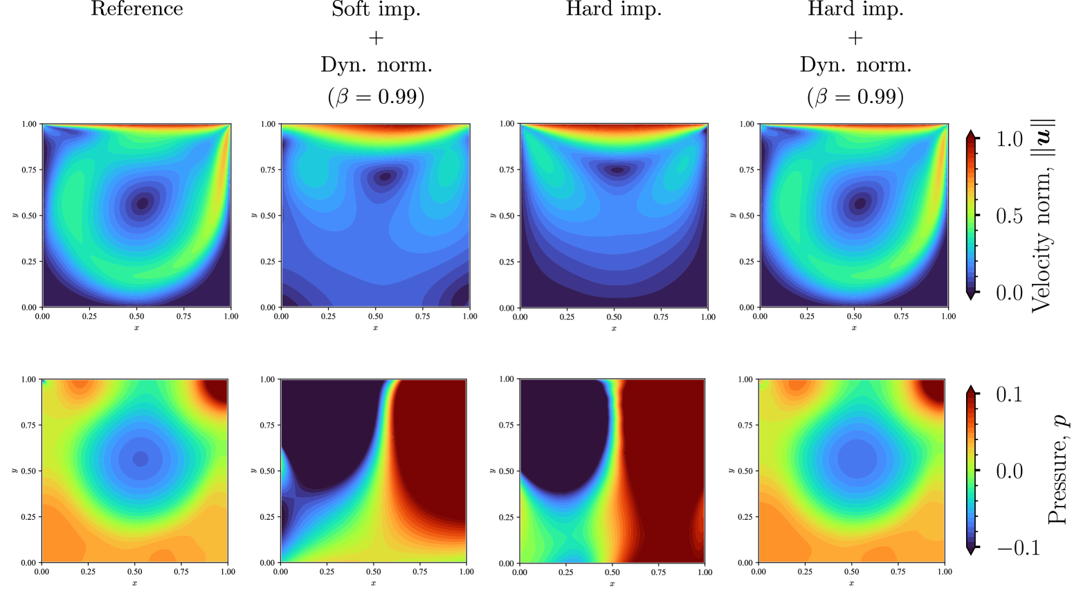
(a) Reference solution, reconstructed velocity, and inferred pressure.

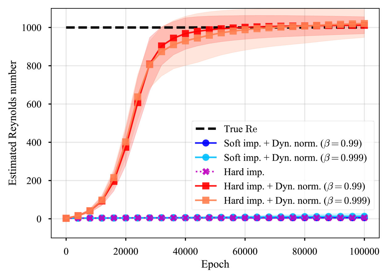
(b) Identification of the Reynolds number (mean and standard deviation over 5 i.i.d. runs).

Figure 9: Shear-driven cavity flow of an incompressible fluid: $\mathit{Re=1,000}$ case. The application of hard imposition alone remains ineffective. Accurate solutions are achieved by combining hard imposition and dynamic normalization.

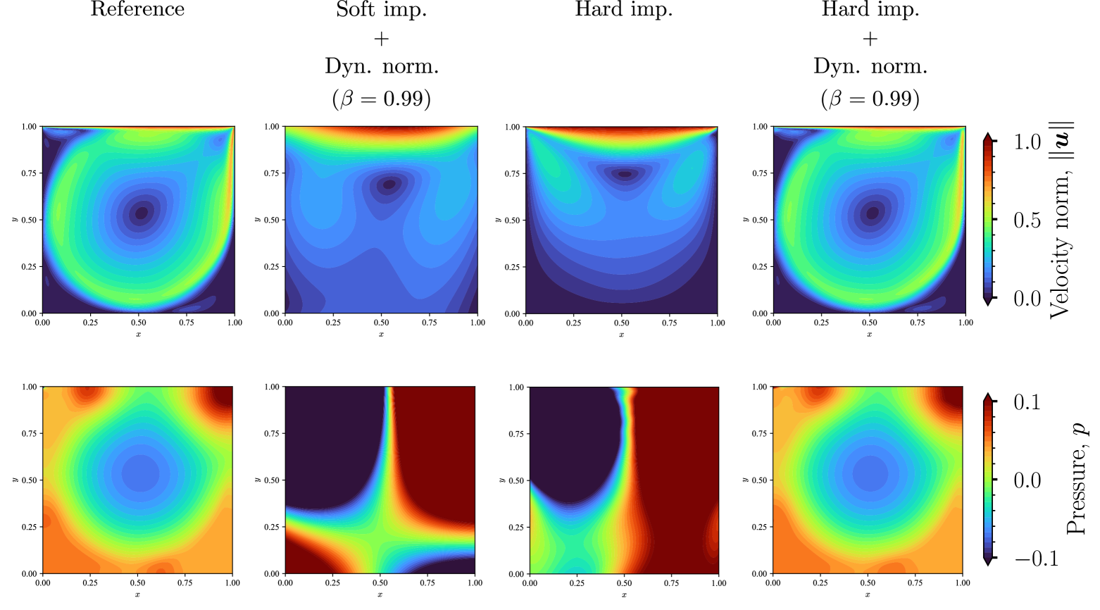
(a) Reference solution, reconstructed velocity, and inferred pressure.

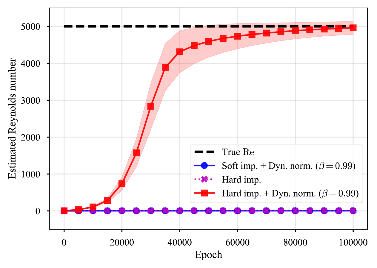
(b) Identification of the Reynolds number (mean and standard deviation over 5 i.i.d. runs).

Figure 10: Shear-driven cavity flow of an incompressible fluid: $\mathit{Re=5,000}$ case. Similar to the $\mathrm{Re}=1,000$ case, the sole application of hard imposition fails. The combination of hard imposition and dynamic normalization achieves accurate inverse analysis.

Figure 9 and 10 present the reconstructed velocity, inferred pressure, and estimated Reynolds number for $\mathrm{Re}=1,000$ and $5,000$ cases, respectively. The importance of boundary condition treatment is highlighted, especially by comparing the velocity norm. Specifically, we observe that the soft imposition fails to recover the velocity field, specifically due to the violation of the prescribed no-slip boundary condition on $\Gamma_{1}\cup\Gamma_{2}\cup\Gamma_{4}$. Consequently, the soft imposition approach also fails to estimate the pressure distribution; the output is inaccurate and physically unrealistic, and the Reynolds number. Given that PINN performance in inverse analysis is highly dependent on boundary condition treatment [46], this failure, primarily attributed to improper boundary condition enforcement, underscores the critical impact of accurate approximate solution construction on inverse analysis.

However, the sole application of the hard imposition is still insufficient. In the third column of Figure 9 and 10, it can be observed that the hard imposition approach precisely satisfies the boundary conditions (Equations (39)–(40)); however, the reconstructed velocity field resembles that of a highly viscous fluid, which is not consistent with the references at the corresponding Reynolds numbers. This discrepancy arises from the inability of the hard imposition alone to balance data and PDE losses, thereby preventing the effective integration of observed data into the network.

In contrast, the combination of hard imposition and dynamic normalization achieves a balance between multiple losses, leading to accurate reconstruction of the velocity field and pressure distribution, as demonstrated in the fourth column of Figure 9 and 10. The Reynolds number is also accurately estimated for both cases. These results convincingly demonstrate the robustness and effectiveness of the hard boundary condition imposition and adaptive weight tuning for inverse problems using PINNs.

3.3 Inverse problem: incompressible flow around an obstacle

Square obstacle case

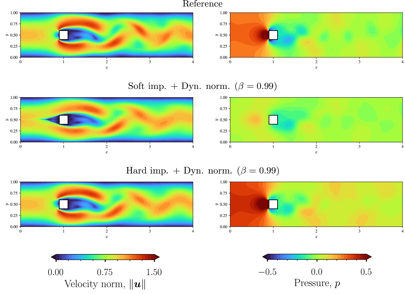
(a) Velocity norm and pressure. (From top to bottom) reference solution, soft and hard impositions with dynamic normalization.

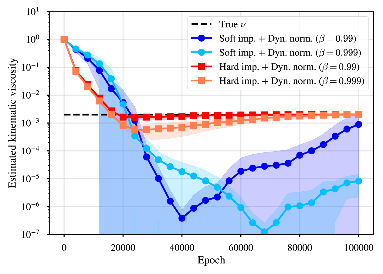
(b) Estimated kinematic viscosity. The solid line and the shaded area represent the mean and the standard deviation over 5 i.i.d. runs, respectively. Results without dynamic normalization are not shown for clarity, as they were significantly worse.

Figure 11: Incompressible flow around an obstacle: square obstacle case. Reconstructed velocity field, inferred pressure, and estimated kinematic viscosity.

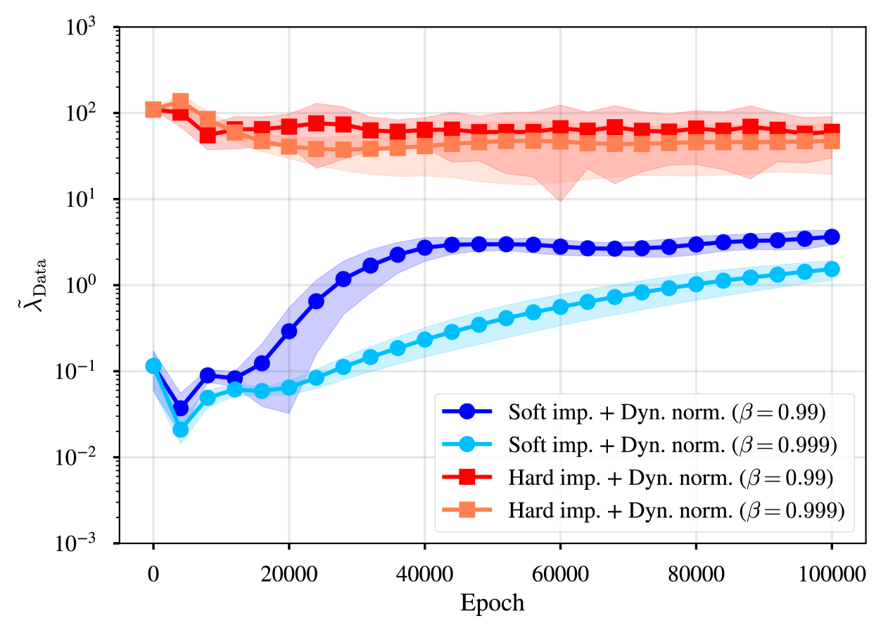
(a) Weight assigned to the data loss, $\tilde{\lambda}_{\text{Data}}$

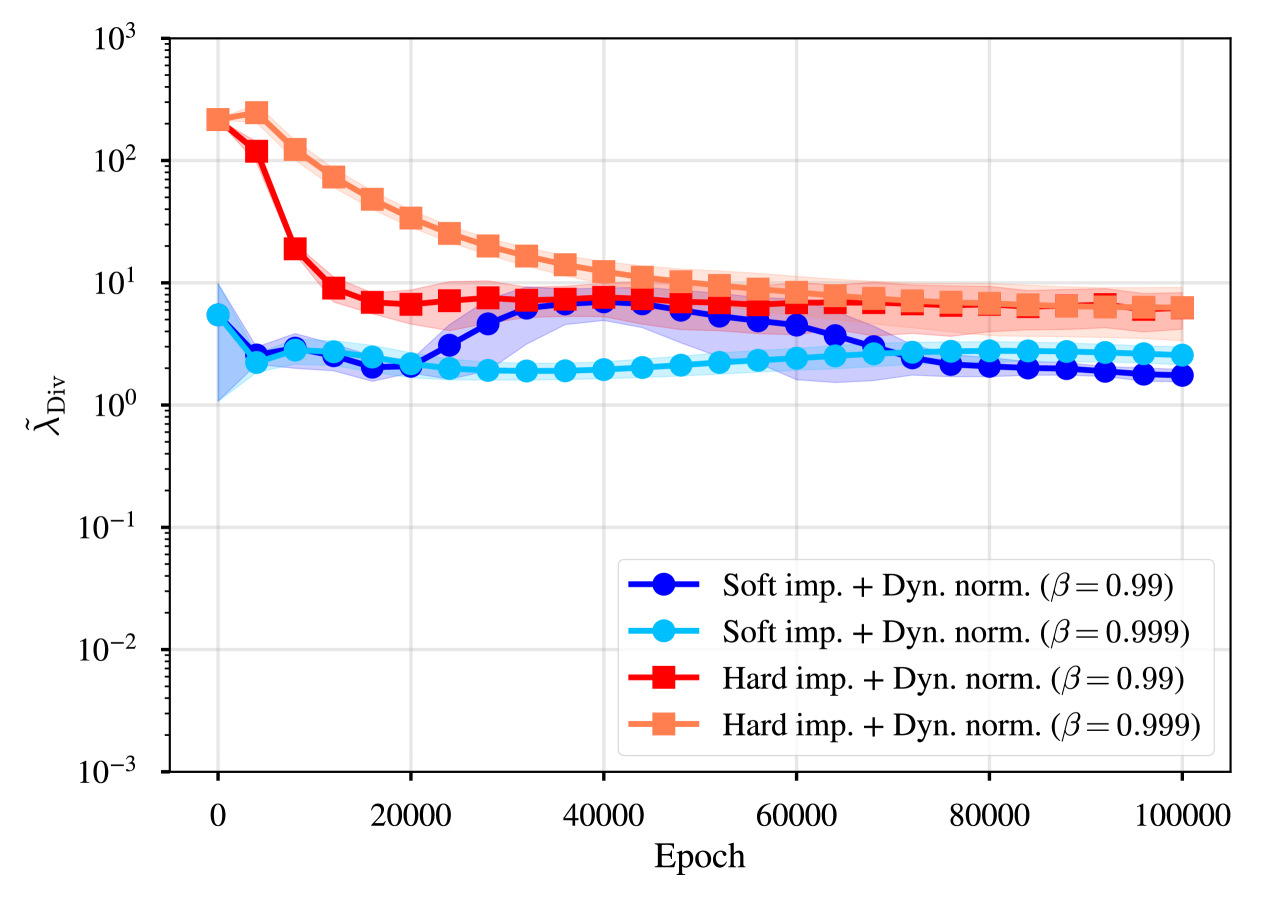
(b) Weight assigned to the divergence loss, $\tilde{\lambda}_{\text{Div}}$

Figure 12: Incompressible flow around an obstacle: square obstacle case. Evolution of the adaptive weights assigned to the data and divergence losses.

Table 3: Incompressible flow around an obstacle: square obstacle case. Estimated kinematic viscosity. Mean and standard deviation over 5 i.i.d. runs are shown. True value is $2\times 10^{-3}\ [\mathrm{m^{2}/s}]$.

Method	Estimated kinematic viscosity [$\mathrm{m^{2}/s}$]
Soft imp.	$7.929\times 10^{-5}\pm 3.051\times 10^{-5}$
Soft imp. + Dyn. norm. ($\beta=0.99$)	$8.939\times 10^{-4}\pm 1.303\times 10^{-3}$
Soft imp. + Dyn. norm. ($\beta=0.999$)	$8.264\times 10^{-6}\pm 6.069\times 10^{-6}$
Hard imp.	$8.501\times 10^{-4}\pm 1.384\times 10^{-3}$
Hard imp. + Dyn. norm. ($\bm{\beta=0.99}$)	$2.038\times 10^{-3}\pm 1.254\times 10^{-4}$
Hard imp. + Dyn. norm. ($\bm{\beta=0.999}$)	$2.008\times 10^{-3}\pm 1.166\times 10^{-4}$

Following [9], we consider an unsteady flow over an obstacle. The governing equations read as:

$$\nabla\cdot\bm{u} =0 \quad\text{in}\quad\Omega\times\mathcal{I},$$ (42)

$$\frac{\partial\bm{u}}{\partial t}+(\bm{u}\cdot\nabla)\bm{u} =-\frac{1}{\rho}\nabla p+\nu\nabla^{2}\bm{u} \quad\text{in}\quad\Omega\times\mathcal{I},$$ (43)

where $\bm{u}=(u,v)^{\top}$ is the velocity [$\mathrm{m/s}$], $p$ is the pressure [$\mathrm{Pa}$], $\rho$ is the density [$\mathrm{kg/m^{3}}$], and $\nu$ is the kinematic viscosity [$\mathrm{m^{2}/s}$]. We set the density and the kinematic viscosity to $\rho=1\ [\mathrm{kg/m^{3}}]$ and $\nu=2\times 10^{-3}\ [\mathrm{m^{2}/s}]$. The domain is $4\ [\mathrm{m}]\times 1\ [\mathrm{m}]$ rectangle with a square obstacle of side length $0.2\ [\mathrm{m}]$ located at $(1,0.5)$. No-slip conditions are applied on the obstacle, top, and bottom boundaries. A parabolic velocity profile with a maximum velocity of $1\ [\mathrm{m/s}]$ is given on the inlet boundary, and a zero-gradient condition is imposed on the outlet. The corresponding Reynolds number is $\mathrm{Re}\sim 100$. The reference solution was obtained through a FDM simulation, employing the same computational scheme as in Section 3.2, with a spatial resolution of $\Delta x=\Delta y=1\times 10^{-2}\ [\mathrm{m}]$ and a time step of $\Delta t=1\times 10^{-3}\ [\mathrm{s}]$. The simulation was executed until the flow reached a periodic state, and a 5-second segment of this periodic flow was extracted as the reference solution. Similar to the cavity flow problem, we consider an inverse problem of identifying the kinematic viscosity $\nu$ and the pressure $p$ from limited observations of the velocity field $\bm{u}$. This study differs from the previous works [9, 70] by considering the entire computational domain, rather than focusing solely on the wake region. This highlights the effect of different boundary condition imposition techniques on the performance of the inverse analysis using PINN. Moreover, in this study, the distance is built based on R-functions [50, 51, 52], which makes it possible to detect interior edges (cylinder boundary), as well as the outer boundary. This treatment was infeasible with the approaches described in [2, 39, 45, 34, 66], as they primarily focused on detecting outer boundaries defined by convex hulls. Collocation points were randomly drawn with $N_{\text{PDE}}=1,024$ and $N_{\text{Data}}=64$ every $0.1\ [\mathrm{s}]$, resulting in a total of $N_{\Omega\times\mathcal{I}}=52,224$ and $N_{\text{Data}\times\mathcal{I}}=3,264$. For soft imposition, $N_{\Gamma_{\text{inlet}}\times\mathcal{I}}=N_{\Gamma_{\text{outlet}}\times\mathcal{I}}=5,151$, $N_{\Gamma_{\text{top}}\times\mathcal{I}}=N_{\Gamma_{\text{bottom}}\times\mathcal{I}}=20,451$, $N_{\Gamma_{\text{cylinder}}\times\mathcal{I}}=4,284$ points were added for the boundary condition enforcement. For this problem, we only employed GELU, as it demonstrated the best performance in previous sections. The Adam optimizer with a learning rate of $1\times 10^{-3}$ was used.

Figure 11 (a) shows the reference, reconstructed velocity, and inferred pressure fields, as well as the estimated kinematic viscosity for the square obstacle case. While the soft imposition demonstrates reasonable agreement with the reference in the wake region, it faces significant challenges in accurately capturing the flow pattern near the obstacle. In particular, the velocity field exhibits non-physical flow separation upstream of the object, with its magnitude being underestimated both near the obstacle and within the wake region. Furthermore, the pressure field shows a non-physical distribution, with the peak point shifted upstream from the obstacle. Conversely, the combination of hard imposition and dynamic normalization captures the flow structure accurately, including the region around the cylinder. Although a slight underestimation of the velocity magnitude is observed in the wake, the discrepancy is considerably smaller than that of the soft imposition. The pressure field, which was not provided to the network, is also inferred with high accuracy, with the peak pressure point correctly located on the obstacle surface. It is important to note that, due to the nature of the incompressible flow, the pressure is determined only up to an additive constant [101]. Therefore, the slight shift observed in the inferred pressure under hard imposition and dynamic normalization is not a concern.

The results of the kinematic viscosity estimation are shown in Figure 11 (b) and summarized in Table 3. Figure 11 (b) reveals that the soft imposition yields highly unstable viscosity estimates, rendering it unsuitable for practical applications. As can be seen in Table 3, the soft imposition, even with dynamic normalization, fails to accurately identify the kinematic viscosity, undershooting the true value by orders of magnitude. In contrast, the combination of hard imposition and dynamic normalization provides stable and accurate viscosity estimates, closely matching the true value. Notably, the estimation error in the viscosity is only 1.9% for $\beta=0.99$ and 0.4% for $\beta=0.999$, where $\beta$ is the decay rate of dynamic normalization. Furthermore, training did not converge in the absence of dynamic normalization, as indicated in Table 3. These findings underscore the critical role of hard boundary condition imposition and dynamic normalization in enhancing the performance of PINNs in inverse analysis. In addition, Figure 12 illustrates the evolution of the adaptive weights assigned to the data and divergence losses. One can observe that the weights are adaptively adjusted from the early stages of training, highlighting the effectiveness of bias-corrected dynamic normalization in balancing the data and divergence losses.

Heart-shaped obstacle case

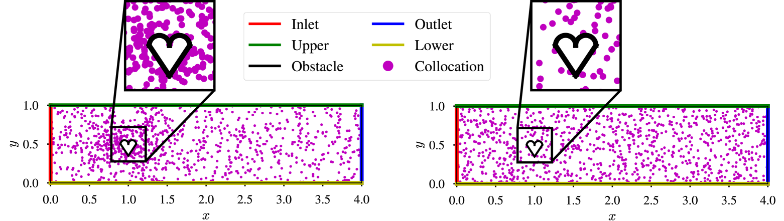
(a) Distribution of collocation points.

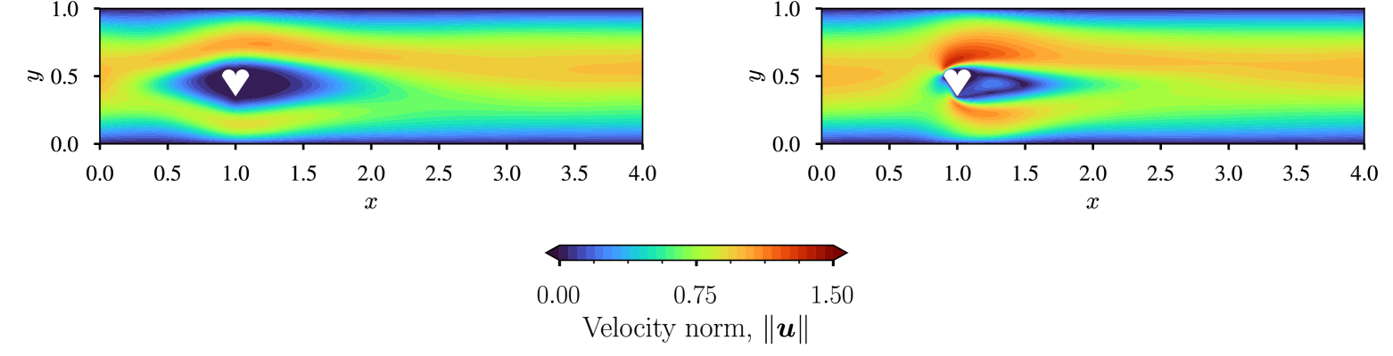
(b) Reconstructed velocity field.

Figure 13: Incompressible flow around an obstacle: heart-shaped obstacle case. Comparison of collocation point sampling strategy. (Left) non-uniform distribution, where FEM nodes are used as collocation points. (Right) uniform distribution, where collocation points are drawn from the uniform probability density.

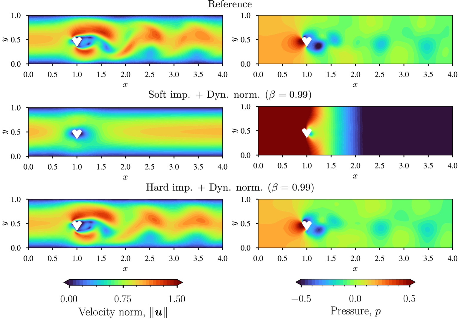
(a) Velocity norm and pressure. (From top to bottom) reference solution, soft and hard impositions with dynamic normalization.

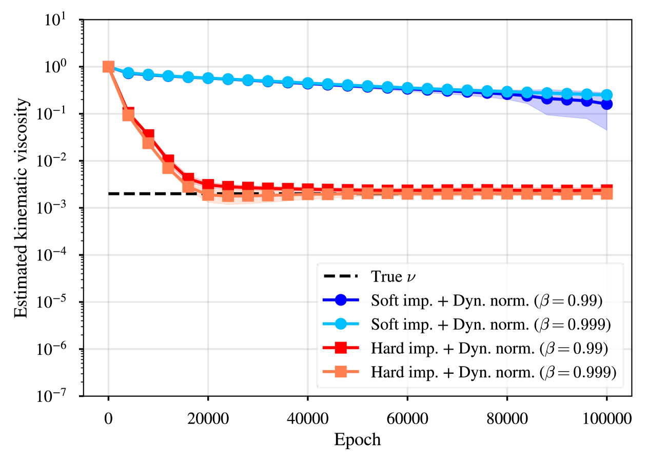
(b) Estimated kinematic viscosity. The solid line and the shaded area represent the mean and the standard deviation over 5 i.i.d. runs, respectively. Results without dynamic normalization are not shown for clarity, as they did not provide satisfactory results.

Figure 14: Incompressible flow around an obstacle: heart-shaped obstacle case. Reconstructed velocity field, inferred pressure, and estimated kinematic viscosity.

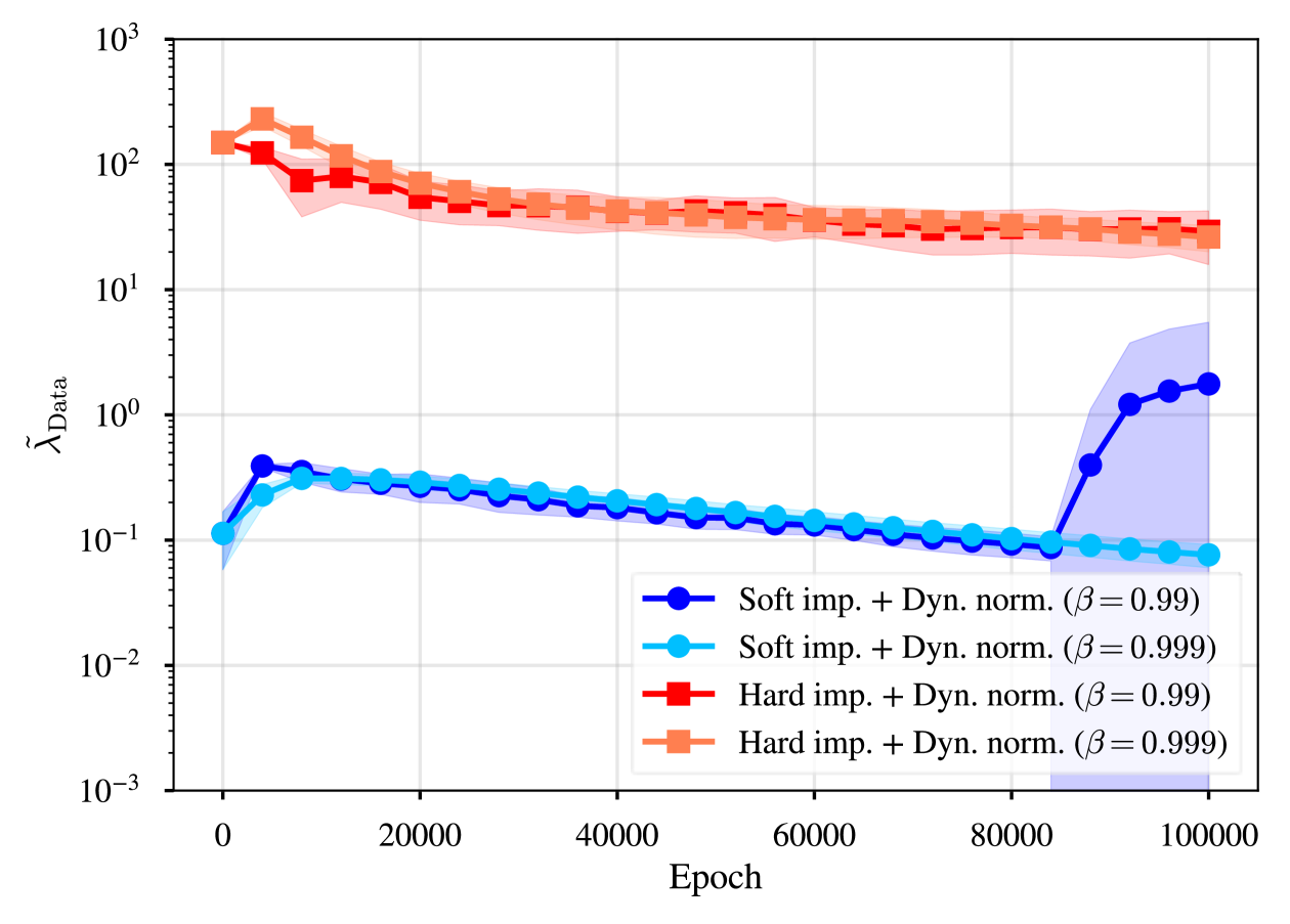
(a) Weight assigned to the data loss, $\tilde{\lambda}_{\text{Data}}$

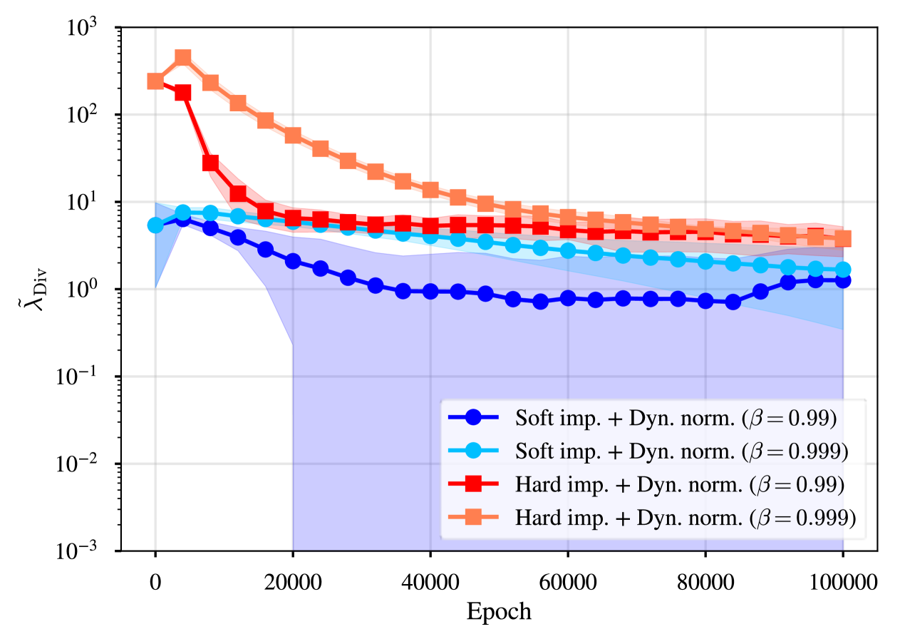
(b) Weight assigned to the divergence loss, $\tilde{\lambda}_{\text{Div}}$

Figure 15: Incompressible flow around an obstacle: heart-shaped obstacle case. Evolution of the adaptive weights assigned to the data and divergence losses.

Table 4: Incompressible flow around an obstacle: heart-shaped obstacle case. Estimated kinematic viscosity. Mean and standard deviation over 5 i.i.d. runs are shown. True value is $2\times 10^{-3}\ [\mathrm{m^{2}/s}]$.

Method	Estimated kinematic viscosity [$\mathrm{m^{2}/s}$]
Soft imp	$4.609\times 10^{-3}\pm 1.038\times 10^{-4}$
Soft imp. + Dyn. norm. ($\beta=0.99$)	$1.611\times 10^{-1}\pm 1.163\times 10^{-1}$
Soft imp. + Dyn. norm. ($\beta=0.999$)	$2.529\times 10^{-1}\pm 2.223\times 10^{-2}$
Hard imp.	$2.532\times 10^{-3}\pm 9.627\times 10^{-4}$
Hard imp. + Dyn. norm. ($\bm{\beta=0.99}$)	$2.369\times 10^{-3}\pm 3.335\times 10^{-4}$
Hard imp. + Dyn. norm. ($\bm{\beta=0.999}$)	$1.999\times 10^{-3}\pm 1.066\times 10^{-4}$

The methodology is further extended to the flow around a heart-shaped obstacle. The governing equations are the same as in the previous case (Equations (42) and (43)). The domain is a $4\ [\mathrm{m}]\times 1\ [\mathrm{m}]$ rectangle, and the square cylinder is replaced with a heart-shaped obstacle. The same kinematic viscosity and boundary conditions are applied, and the geometric parameters are chosen so that the same Reynolds number is maintained. The reference solution was obtained using a P2/P1 finite element method [102] on a triangular mesh. The P2/P1 interpolation was chosen to satisfy the inf-sup condition, ensuring the stability of the numerical solutions [103]. The mesh was progressively refined towards the obstacle, resulting in minimum, maximum, and average element lengths of $3.5\times 10^{-3}\ [\mathrm{m}]$, $2.4\times 10^{-2}\ [\mathrm{m}]$, $1.2\times 10^{-2}\ [\mathrm{m}]$, respectively. The problem was solved with varying mesh resolutions, confirming the convergence of the numerical results with the current resolution. The flow exhibits periodic, yet asymmetric behavior, attributed to the obstacle’s geometry. The obtained numerical solution is used as the reference for the inverse analysis. The same number of collocation points and identical settings for the learning rate, dynamic normalization, and activation function were used as in the square obstacle case.

In the computational fluid dynamics community, it is common practice to employ dense and refined meshes near obstacles with complex geometries so that one can accurately capture steep gradients of the flow. Motivated by this, we first compared the PINN’s performance using collocation points taken from the finite element nodes (increased density near the obstacle) and those uniformly drawn from the domain (see Figure 13 (a)). For this preliminary test, we used hard imposition approach without dynamic normalization to focus on the effect of the collocation point distribution. Velocity reconstruction results are presented in Figure 14 (b). Although both are not quite satisfactory, the uniform distribution of collocation points yields better results. This result is fairly natural from Monte Carlo perspective, as each collocation point holds a representative volume to discretize the integrals in the loss function. Indeed, low-discrepancy sequences (e.g., lattice) are known to generally facilitate quicker convergence [62]. For non-uniform distributions, techniques such as volumetric averaging [104] can be incorporated to adjust the representative volume based on collocation point density. However, a comprehensive study of non-uniform collocation points is beyond the scope of this work. Based on this observation, we proceed with uniformly distributed collocation points for the problem with the heart-shaped obstacle.

Figure 14 shows the velocity field, pressure, and estimated kinematic viscosity obtained using the soft and hard impositions with dynamic normalization. From Figure 14 (a), one can observe that the solution obtained with soft imposition, even with dynamic normalization, does not exhibit the shedding structure, resembling a highly viscous or steady flow. This observation aligns with [105], and is attributed to improper boundary condition treatment. Results with the hard imposition clearly reproduce the vortex shedding, and the pressure distribution is also accurately inferred. The kinematic viscosity estimation is illustrated in Figure 14 (b) and summarized in Table 4. One can further confirm that the unobserved viscosity is accurately identified by the combination of hard imposition and dynamic normalization. Notably, neither distance function-based enforcement nor dynamic normalization alone is sufficient; both techniques are necessary to achieve accurate results. Once again, the distance field constructed upon R-functions [50, 51, 52] enables the detection of both outer and interior boundaries, and further extends to non-convex geometries, such as the heart-shaped domain in this problem. This capability is a unique feature of R-function-based distance fields, which approaches in [2, 39, 45, 34, 66] cannot handle, as they implicitly assume convex hull boundaries. Furthermore, Figure 15 illustrates the evolution of the adaptive weights built by bias-corrected dynamic normalization. The weights exhibit stable behavior when combined with the distance functions, which is similar to the behavior of adaptive activation functions observed in the channel flow problems by Sun et al. [39]. These results suggest that hard boundary condition enforcement contributes to the stability of the adaptive weights.

4 Conclusion

In this study, we investigated the impact of boundary condition imposition techniques on the performance of physics-informed neural networks for both forward and inverse problems of partial differential equations. Although penalty-based soft enforcement is prevalent in the literature, its performance is highly sensitive to the weight parameter, requiring very careful tuning [10, 40]. In contrast, distance function-based hard enforcement directly encodes the boundary conditions into the approximate function structure, ensuring that the solution inherently satisfies the prescribed conditions. In addition, we have reviewed the properties of R-functions [50, 51, 52, 64] while exploring the use of distance functions in the context of boundary value problems. In the framework of R-functions, the distance field is normalized, providing a smooth and differentiable representation of distance and unit normal vectors on the boundaries. These properties are crucial for applications to homogeneous/inhomogeneous Dirichlet, Neumann, and mixed boundary conditions [55, 56, 57, 46, 58] and enable the detection of arbitrary polygonal and non-convex boundaries, overcoming limitations of other (non-normalized) distance function-based approaches [2, 39, 45, 66].

The effectiveness of distance-based hard imposition was first verified with a forward problem of the Poisson equation and subsequently extended to inverse problems of incompressible flow in a cavity and around an obstacle. For forward problems, soft imposition approach quickly reached a plateau, which is consistent result with [39]. In contrast, hard imposition outperformed soft enforcement across various activation functions, achieving faster convergence and lower error. The same architecture was then applied to inverse problems, however, we found that the sole application of hard imposition to explicitly enforce the boundary conditions was insufficient to achieve accurate inverse analysis. To address this, we introduced dynamic normalization [47], which adaptively adjusts the weights assigned to the data and PDE losses, and combined it with hard imposition. The proposed framework, incorporating hard imposition (based on distance functions) and dynamic normalization (adaptive weight tuning), provided a robust and efficient inverse analysis approach. This study underscores the importance of boundary condition treatment and the efficacy of adaptive weight tuning in improving the performance of PINNs, particularly for inverse problems.

The presented method, however, is not without limitations. For example, the neural network structure is a simple MLP, and advanced architectures and preprocessing techniques, such as basis transformation [33, 34], domain decomposition [35, 37, 36], and mixed-variable formulations [106, 84] could be explored to capture the complex flow structures more effectively.

Acknowledgements

This work was supported by Japan Society for the Promotion of Science (JSPS) KAKENHI Grant Number JP23KK0182, JP23K17807, JP23K26356, JP23K24857, JP23KJ1685, and Japan Science and Technology Agency (JST) Support for Pioneering Research Initiated by the Next Generation (SPRING) Grant Number JPMJSP2136.

CRediT author contribution statement

S. Deguchi: Conceptualization, Methodology, Validation, Formal analysis, Investigation, Data Curation, Writing - Original Draft, Funding acquisition.

M. Asai: Conceptualization, Methodology, Resources, Writing - Review & Editing, Supervision, Project administration, Funding acquisition.

Data availability

The code will be made available at: https://github.com/ShotaDeguchi/PINN_HardBC_DynNorm upon publication.

Conflict of interest

The authors have no competing interests to declare that are relevant to the content of this article.

Appendix A Numerical study on several improvement techniques

Several techniques have been proposed to improve the performance of PINN. In this section, we report numerical results for some of these techniques applied to the Poisson equation with mixed boundary conditions (described in Section 3.1).

Adaptive activation function

There have been many studies on adaptive activation functions in the literature of neural networks [107, 86]. Similarly, Jagtap et al. [83, 88] proposed adaptive activation functions in the context of PINNs, in which the forward pass is modified as follows:

$$\mathbf{z}^{(l)}=\sigma^{(l)}\left(s^{(l)}\left(\mathbf{W}^{(l)}\mathbf{z}^{(l-1)}+\mathbf{b}^{(l)}\right)\right),$$ (A.1)

where a learnable scaling factor $s^{(l)}$ is introduced in each layer. Equation (A.1) is known as layer-wise locally adaptive activation function (L-LAAF) [88]. With this modification, the set of trainable parameters becomes $\bm{\theta}=\left\{\mathbf{W}^{(l)},\bm{b}^{(l)},s^{(l)}\right\}_{l=1}^{L}\setminus\left\{s^{(L)}\right\}$. The core idea behind this modification is to adaptively adjust the slope of the activation functions. Specifically, backpropagated gradients are amplified if $s^{(l)}\geq 1$ and attenuated if $s^{(l)}<1$. To encourage $s^{(l)}$ to increase, thereby accelerating optimization, Jagtap et al. [88] introduced the following slope recovery term into the loss function:

$$\mathcal{L}_{\text{SR}}=\frac{1}{1/(L-1)\sum_{l=1}^{L-1}\exp\left(s^{(l)}\right)}.$$ (A.2)

As $\mathcal{L}_{\text{SR}}$ decreases, $s^{(l)}$ increase, which enhances the gradients and accelerates convergence.

Gradient enhancement

Yu et al. [25] proposed a gradient enhancement technique, termed gPINN, where an additional loss term is introduced to penalize the derivatives of the PDE residual so that they approach zero. In particular, they introduced the following gradient enhancement term:

$$\mathcal{L}_{\text{GE}}=\sum_{k=1}^{d}\int_{\Omega}\left|\frac{\partial}{\partial x_{k}}\left(-\nabla^{2}\hat{u}\left(\bm{x};\bm{\theta}\right)-f\left(\bm{x}\right)\right)\right|^{2}\,d\bm{x}.$$ (A.3)

While higher-order derivatives can be included to further enforce smoothness, the computational cost increases rapidly with the order of differentiation. Moreover, the effectiveness of gradient enhancement is highly sensitive to the weight $\lambda_{\text{GE}}$, and improper tuning of $\lambda_{\text{GE}}$ may lead to degraded performance, whereas gPINN could be effective for scarce data and help prevent oscillation due to its smoothing effect [108, 109].

Self-adaptive soft attention mechanism

McClenny & Braga-Neto [90] proposed self-adaptive PINN (SA-PINN), in which a set of learnable weights is introduced to adaptively determine the importance of each collocation point. In SA-PINN, the loss function is modified as follows:

$$\mathcal{L}\left(\bm{\theta},\bm{\lambda}\right) =\mathcal{L}_{\text{PDE}}\left(\bm{\theta},\bm{\lambda}_{\text{PDE}}\right)+\mathcal{L}_{\text{BC}}\left(\bm{\theta},\bm{\lambda}_{\text{DBC}},\bm{\lambda}_{\text{NBC}}\right)+\mathcal{L}_{\text{Data}}\left(\bm{\theta},\bm{\lambda}_{\text{Data}}\right),$$ (A.4)

$$\mathcal{L}_{\text{PDE}}\left(\bm{\theta},\bm{\lambda}_{\text{PDE}}\right) =\frac{1}{N_{\text{PDE}}}\sum_{i=1}^{N_{\text{PDE}}}m\left(\lambda_{\text{PDE},i}\right)\left|-\nabla^{2}\hat{u}\left(\bm{x}_{i};\bm{\theta}\right)-f\left(\bm{x}_{i}\right)\right|^{2},$$ (A.5)

$$\begin{split}\mathcal{L}_{\text{BC}}\left(\bm{\theta},\bm{\lambda}_{\text{DBC}},\bm{\lambda}_{\text{NBC}}\right)&=\frac{1}{N_{\text{DBC}}}\sum_{i=1}^{N_{\text{DBC}}}m\left(\lambda_{\text{DBC},i}\right)\left|\hat{u}(\bm{x}_{i};\bm{\theta})-g_{D}(\bm{x}_{i})\right|^{2}\\ &\quad+\frac{1}{N_{\text{NBC}}}\sum_{i=1}^{N_{\text{NBC}}}m\left(\lambda_{\text{NBC},i}\right)\left|\bm{n}\cdot\nabla\hat{u}(\bm{x}_{i};\bm{\theta})-g_{N}(\bm{x}_{i})\right|^{2},\end{split}$$ (A.6)

$$\mathcal{L}_{\text{Data}}\left(\bm{\theta},\bm{\lambda}_{\text{Data}}\right) =\frac{1}{N_{\text{Data}}}\sum_{i=1}^{N_{\text{Data}}}m\left(\lambda_{\text{Data},i}\right)\left|\hat{u}\left(\bm{x}_{i};\bm{\theta}\right)-u_{\text{Data}}\left(\bm{x}_{i}\right)\right|^{2},$$ (A.7)

where $\bm{\lambda}=\left\{\bm{\lambda}_{\text{PDE}},\bm{\lambda}_{\text{DBC}},\bm{\lambda}_{\text{NBC}},\bm{\lambda}_{\text{Data}}\right\}$ is a set of non-negative learnable weights assigned to each collocation point. $m:\mathbb{R}_{\geq 0}\to\mathbb{R}_{>0}$ is a smooth, strictly monotonically increasing function, typically chosen as $m\left(\cdot\right)=\max\left(0,\cdot\right)^{2}$ [90, 110]. The training of the self-adaptive PINN is formulated as $\min_{\bm{\theta}}\max_{\bm{\lambda}}\mathcal{L}\left(\bm{\theta},\bm{\lambda}\right)$, where $\bm{\theta}$ is updated using gradient descent, while $\bm{\lambda}$ is updated by gradient ascent algorithm:

$$\bm{\theta}^{(n+1)} \leftarrow\bm{\theta}^{(n)}-\eta_{\bm{\theta}}\nabla_{\bm{\theta}}\mathcal{L}\left(\bm{\theta},\bm{\lambda}\right),$$ (A.8)

$$\bm{\lambda}^{(n+1)} \leftarrow\bm{\lambda}^{(n)}+\eta_{\bm{\lambda}}\nabla_{\bm{\lambda}}\mathcal{L}\left(\bm{\theta},\bm{\lambda}\right).$$ (A.9)

Here, $\eta_{\bm{\theta}}$ and $\eta_{\bm{\lambda}}$ are the learning rates for $\bm{\theta}$ and $\bm{\lambda}$, respectively. In [90], authors recommend using a larger learning rate for $\bm{\lambda}$ compared to $\bm{\theta}$, i.e., $\eta_{\bm{\lambda}}=c_{\text{SA}}\eta_{\bm{\theta}}$, for some hyperparameter $c_{\text{SA}}\geq 1$. Self-adaptive PINN has been applied to various domains, such as infection dynamics [110] and seismic wave modeling [111].

Table A.1: Poisson equation with mixed boundary conditions: homogeneous Neumann condition case (described in Section 3.1). Comparison of L-LAAF [88], gPINN [25], and SA-PINN [90]. Relative $L^{2}$ error (mean and standard error) using GELU activation function. All values are scaled by $10^{-3}$ for the consistency with Table 1.

(a) L-LAAF

$\lambda_{\text{SR}}$	Rel. $L^{2}$ Err.
$10^{-2}$	$26.69\pm 1.09$
$10^{-1}$	$22.24\pm 3.46$
$10^{0}$	$31.51\pm 4.81$
$10^{1}$	$33.76\pm 4.81$
$10^{2}$	$70.99\pm 39.03$

(b) gPINN

$\lambda_{\text{GE}}$	Rel. $L^{2}$ Err.
$10^{-8}$	$24.46\pm 1.92$
$10^{-6}$	$27.41\pm 0.27$
$10^{-4}$	$27.44\pm 0.20$
$10^{-2}$	$25.33\pm 2.58$
$10^{0}$	$50.12\pm 2.48$

(c) SA-PINN

$c_{\text{SA}}$	Rel. $L^{2}$ Err.
$10^{-2}$	$26.42\pm 0.98$
$10^{-1}$	$27.66\pm 0.29$
$10^{0}$	$33.96\pm 3.30$
$10^{1}$	$264.84\pm 13.22$
$10^{2}$	$673.34\pm 8.47$

(d) SA-PINN^†

$c_{\text{SA}}$	Rel. $L^{2}$ Err.
$10^{-2}$	$27.28\pm 0.51$
$10^{-1}$	$27.43\pm 0.88$
$10^{0}$	$22.26\pm 2.48$
$10^{1}$	$178.51\pm 14.38$
$10^{2}$	$641.24\pm 4.83$

Table A.1 summarizes the relative $L^{2}$ error with L-LAAF [88], gPINN [25], and SA-PINN [90] for the Poisson equation problem with inhomogeneous Dirichlet and homogeneous Neumann conditions. The problem setup is the same as that in Section 3.1, and the hyperparameters are selected based on the numerical experiments in the original papers and their recommendations described therein. For SA-PINN, we considered two distinct strategies: one where both $\bm{\theta}$ and $\bm{\lambda}$ are updated throughout the optimization (SA-PINN), and the other where a two-stage optimization is employed (SA-PINN^†). In the latter case, $\bm{\theta}$ and $\bm{\lambda}$ were jointly optimized for the first half of the total training epochs, after which $\bm{\lambda}$ was frozen, and only $\bm{\theta}$ was updated for the remaining epochs, following [90]. The results suggest that these methods do not consistently yield substantial improvements, and their effectiveness is highly sensitive to the hyperparameters.

Appendix B Numerical study on normalization orders in distance functions

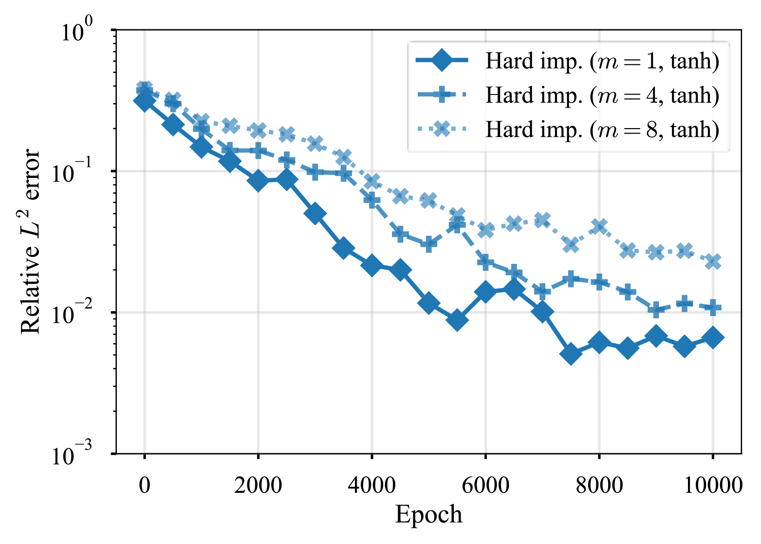
(a) tanh

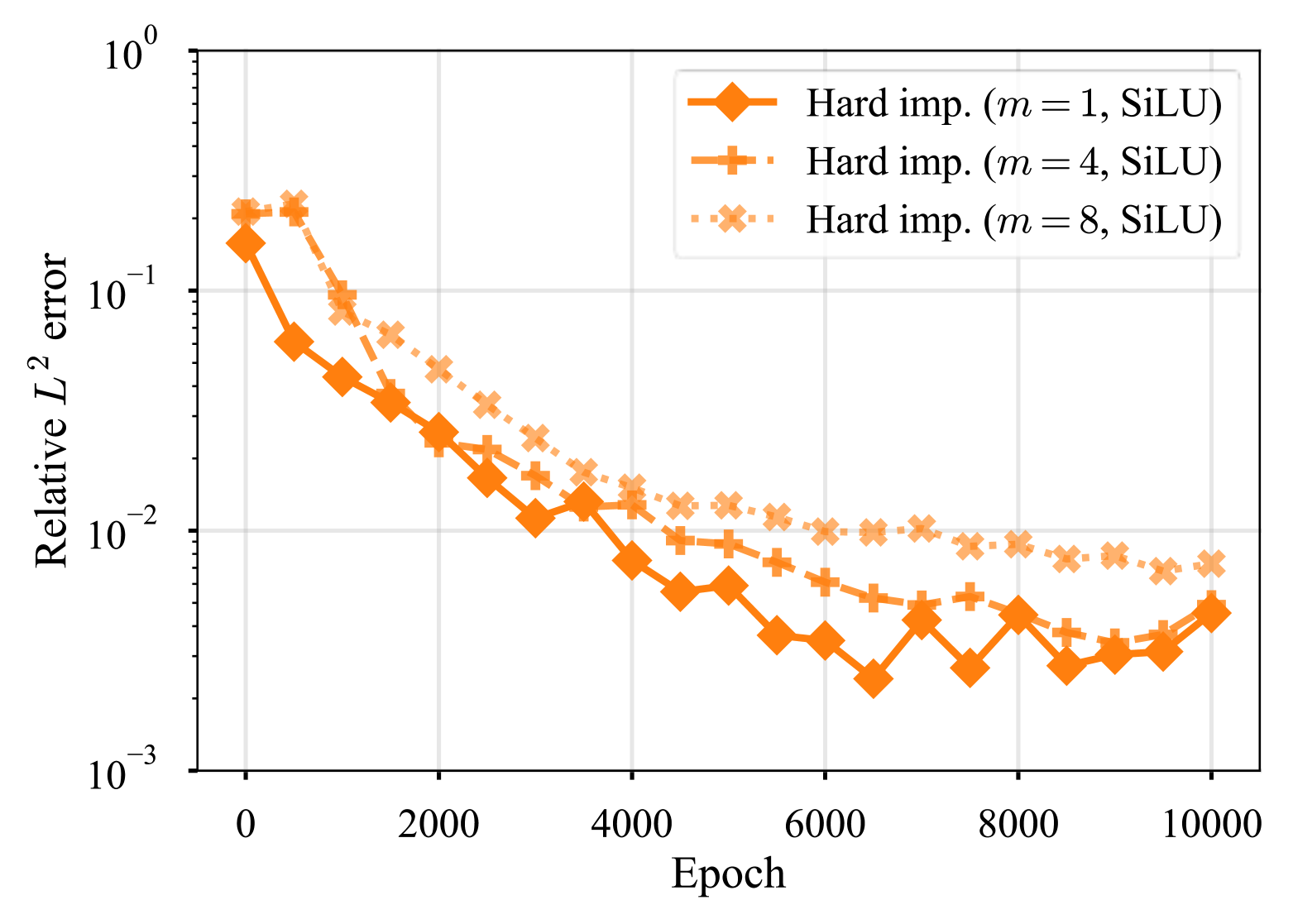
(b) SiLU

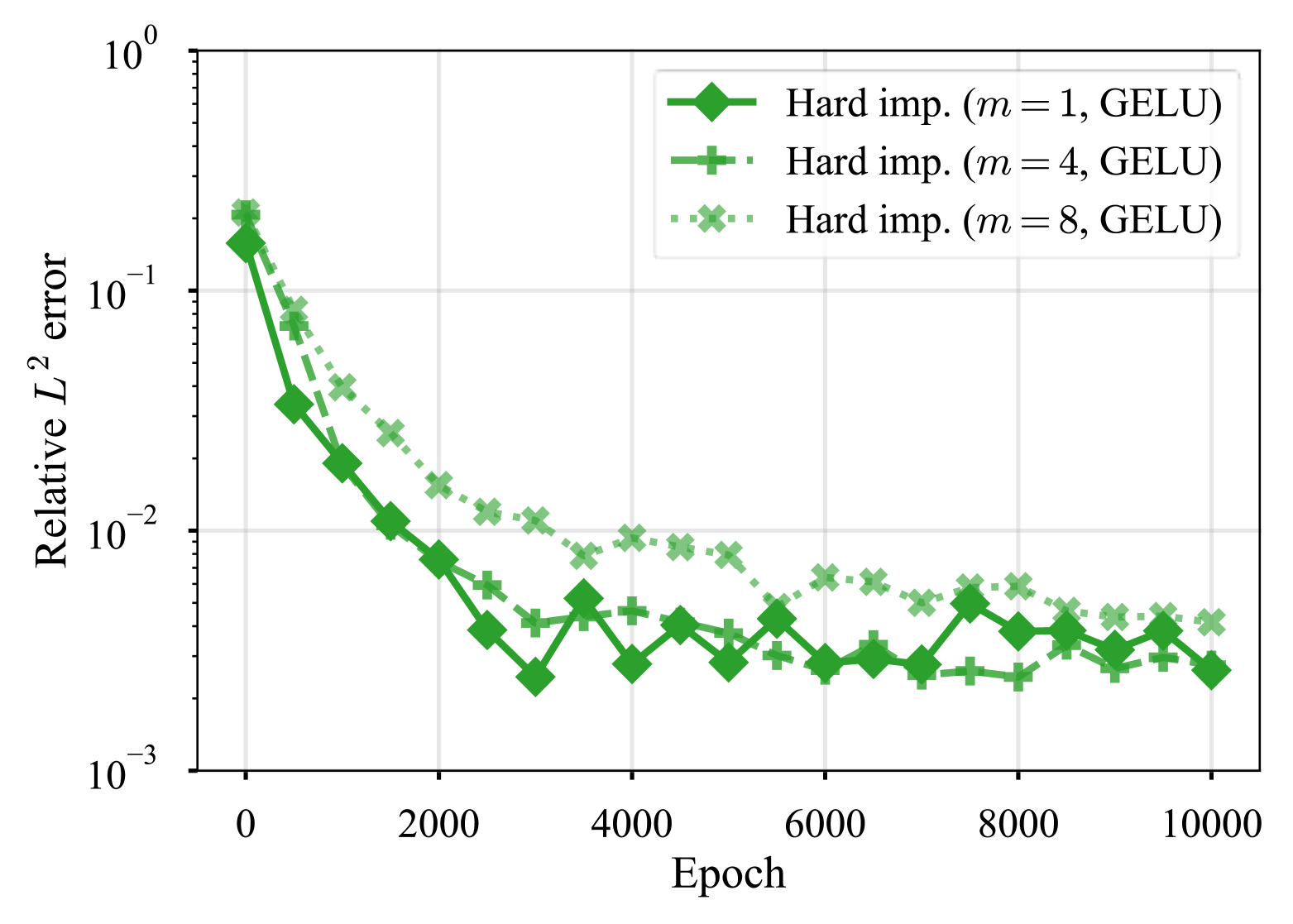
(c) GELU

Figure B.1: Poisson equation with mixed boundary conditions: homogeneous Neumann condition case (described in Section 3.1). Relative $L^{2}$ error of the approximate solution with different normalization orders $m$. Only the mean over 5 i.i.d. runs is shown, and results with $m=2$ are omitted for clarity, as they show similar behavior to $m=1$.

Table B.1: Poisson equation with mixed boundary conditions: homogeneous Neumann condition case (described in Section 3.1). Relative $L^{2}$ error (mean and standard error over 5 independent runs with i.i.d. initialization, scaled by $10^{-3}$) of approximate solution with different normalization orders $m$.

Activation function	$m=1$	$m=2$	$m=4$	$m=8$
tanh	$6.65\pm 2.08$	$14.27\pm 1.68$	$10.82\pm 1.52$	$22.92\pm 2.37$
SiLU	$4.54\pm 1.05$	$5.69\pm 1.24$	$4.92\pm 1.49$	$7.29\pm 2.08$
GELU	$2.62\pm 0.21$	$3.25\pm 0.70$	$2.75\pm 0.23$	$4.15\pm 0.94$

In [46, 58], the behavior of the Laplacian of the ADFs is discussed analytically. Here, we numerically investigate the influence of the normalization order $m$ of the distance functions on the convergence of PINN solutions. Specifically, we consider the Poisson equation problem (described in Section 3.1) as an example. Figure B.1 illustrates the error with different activation functions and normalization orders. The results, summarized in Table B.1, indicate a clear trend: as the normalization order $m$ increases, the convergence of PINN solutions deteriorates for all tested activation functions, although the extent of the degradation varies.

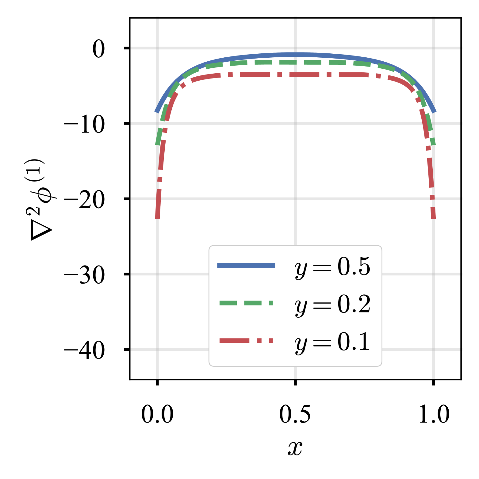
(a) $m=1$

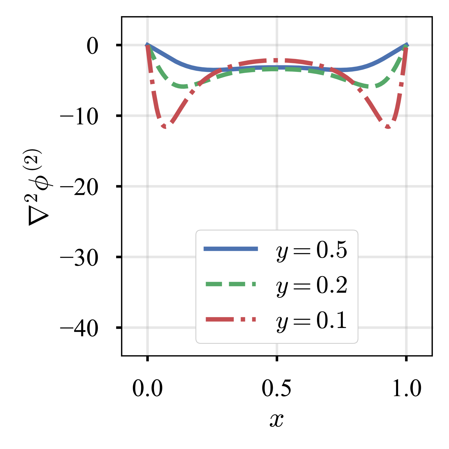
(b) $m=2$

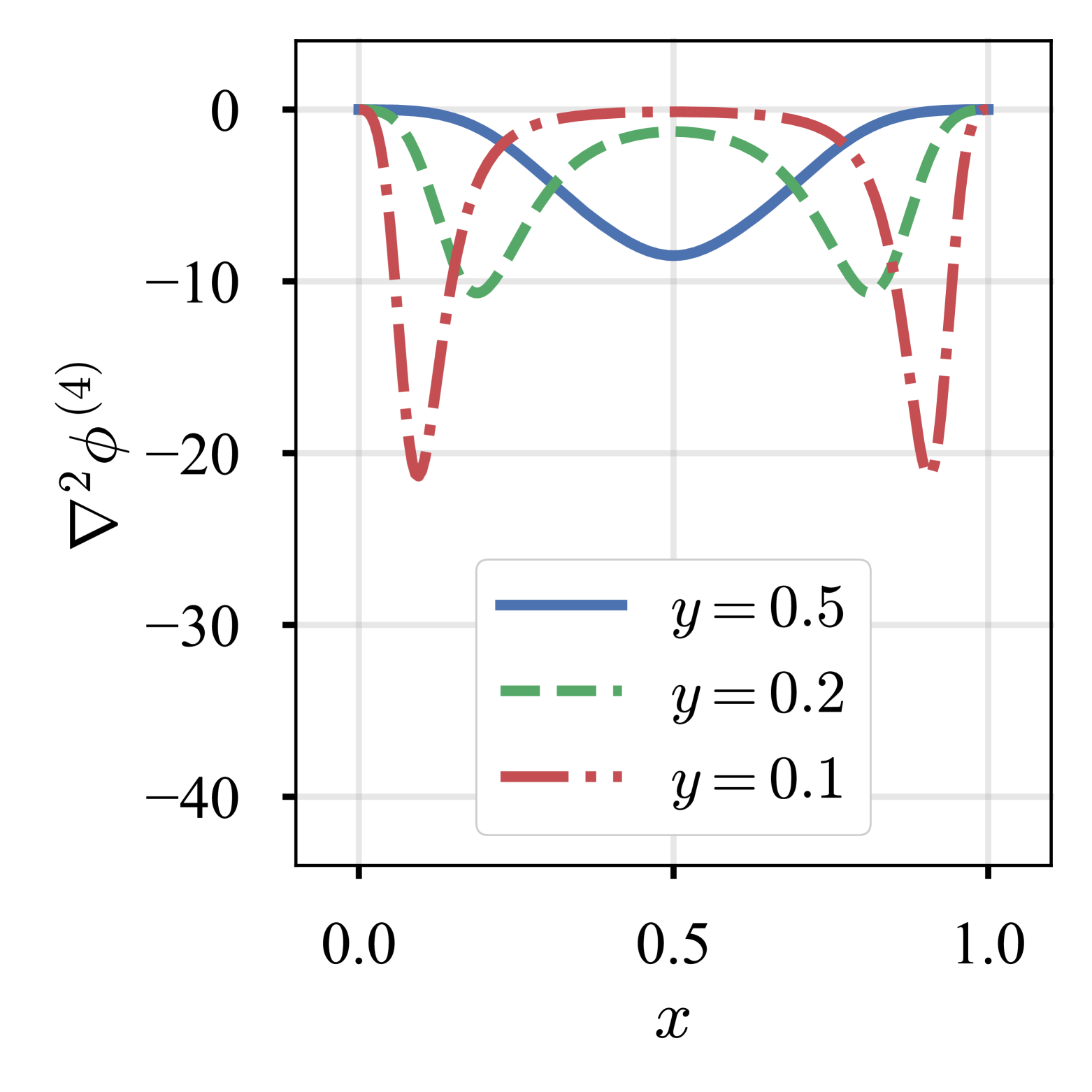
(c) $m=4$

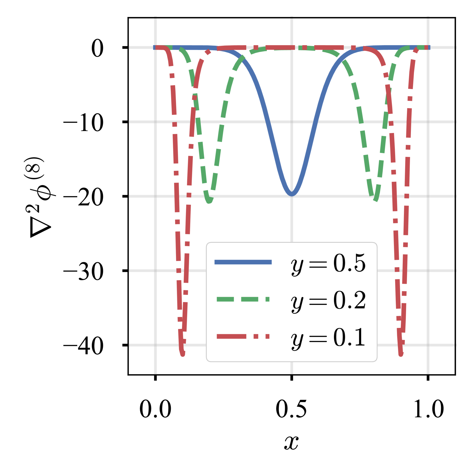
(d) $m=8$

Figure B.2: Laplacian of the normalized ADFs to a unit square (slice). Slice along $y=0.5,0.2,0.1$ are shown. As $m$ increases, the oscillatory behavior near the boundary becomes more pronounced.

To understand the reason behind this behavior, we examine the Laplacian of the ADFs over a unit square with various normalization orders $m$, as depicted in Figure B.2. It is evident that the Laplacian $\nabla^{2}\phi^{(m)}$ exhibits an oscillatory behavior particularly near the boundary, as the normalization order $m$ is increased. Simplifying the problem to the Poisson equation with the homogeneous Dirichlet boundary condition, the approximate solution is defined as $\tilde{u}=\bar{g}_{D}+\phi^{(m)}\hat{u}$ (setting $\bar{g}_{D}=0$ in Equation (15)), where its Laplacian is given by:

$$\nabla^{2}\tilde{u} =\nabla\cdot\nabla\left(\phi^{(m)}\hat{u}\right)$$ (B.1)

$$=\nabla\cdot\left(\hat{u}\nabla\phi^{(m)}+\phi^{(m)}\nabla\hat{u}\right)$$ (B.2)

$$=\hat{u}\nabla^{2}\phi^{(m)}+\phi^{(m)}\nabla^{2}\hat{u}+2\left(\nabla\hat{u},\nabla\phi^{(m)}\right),$$ (B.3)

where $\left(\cdot,\cdot\right)$ denotes the inner product. The presence of $\nabla^{2}\phi^{(m)}$ in $\nabla^{2}\tilde{u}$ suggests a high possibility that $\nabla^{2}\tilde{u}$ inherits the oscillatory nature of $\nabla^{2}\phi^{(m)}$, potentially resulting in the degraded convergence observed in Figure B.1 and Table B.1. This implies that the precise representation of the distance (i.e., higher $m$) is not necessarily advantageous or beneficial; rather, the normalization order $m$ should be kept moderate so as not to require $\hat{u}$ to compensate for the near-boundary oscillations $\nabla^{2}\phi^{(m)}$ may induce, especially when the second derivative appears in the problem of interest.

In order to verify that this is not a special case for a square domain, we also conducted the same analysis for an annulus, $\Omega=\{(r,\varphi)\mid 0.5\leq r\leq 1,0\leq\varphi\leq 2\pi\}$. We applied the method of manufactured solutions to obtain the reference (analytical) solution and source:

$$u =\cos\left(2\pi c_{1}r\right)\sin\left(c_{2}\varphi\right),$$ (B.4)

$$f =\frac{2\pi c_{1}}{r}\sin\left(2\pi c_{1}r\right)\sin\left(c_{2}\varphi\right)+\left(\left(2\pi c_{1}\right)^{2}+\left(\frac{c_{2}}{r}\right)^{2}\right)\cos\left(2\pi c_{1}r\right)\sin\left(c_{2}\varphi\right),$$ (B.5)

where we choose $\left(c_{1},c_{2}\right)=\left(1,2\right)$ and $N_{\text{PDE}}=4,096$. Figure B.3 shows the illustrative results and Table B.2 summarizes the relative $L^{2}$ error with different normalization orders $m$ for the hard imposition. Although SiLU achieves the lowest error with $m=2$, the overall trend is consistent with the square domain case, and the convergence deteriorates as $m$ increases.

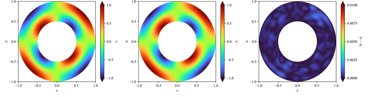
(a) Hard imposition ($m=1$, GELU). Relative $L^{2}$ error: $7.36\times 10^{-4}$.

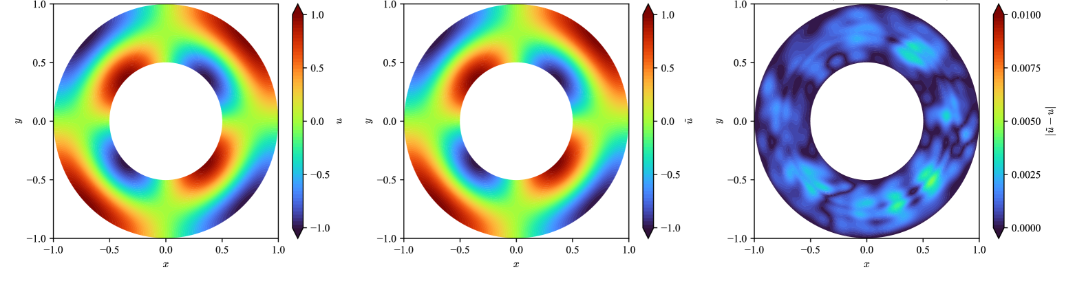
(b) Hard imposition ($m=8$, GELU). Relative $L^{2}$ error: $2.48\times 10^{-3}$.

Figure B.3: Poisson equation on an annulus. (From left to right) reference solution obtained by the method of manufactured solution, approximate solution, and absolute error against the reference solution.

Table B.2: Poisson equation on an annulus. Relative $L^{2}$ error of the approximate solution with different normalization orders $m$. Mean and standard error over 5 independent runs with i.i.d. initialization. All values are scaled by $10^{-3}$.

Activation function	$m=1$	$m=2$	$m=4$	$m=8$
tanh	$0.26\pm 0.04$	$0.49\pm 0.12$	$0.45\pm 0.05$	$0.81\pm 0.06$
SiLU	$1.64\pm 0.45$	$1.34\pm 0.14$	$2.69\pm 0.50$	$5.90\pm 1.08$
GELU	$0.70\pm 0.10$	$1.06\pm 0.18$	$1.13\pm 0.06$	$1.61\pm 0.29$

References

- [1] M. W. M. G. Dissanayake and N. Phan-Thien. Neural-network-based approximations for solving partial differential equations. Communications in Numerical Methods in Engineering, 10(3):195–201, 1994.
- [2] I.E. Lagaris, A. Likas, and D.I. Fotiadis. Artificial neural networks for solving ordinary and partial differential equations. IEEE Transactions on Neural Networks, 9(5):987–1000, 1998.
- [3] Thananchai Leephakpreeda. Novel determination of differential-equation solutions: universal approximation method. Journal of Computational and Applied Mathematics, 146(2):443–457, 2002.
- [4] Kevin Stanley McFall and James Robert Mahan. Artificial neural network method for solution of boundary value problems with exact satisfaction of arbitrary boundary conditions. IEEE Transactions on Neural Networks, 20(8):1221–1233, 2009.
- [5] Alejandro Barredo Arrieta, Natalia DÃaz-RodrÃguez, Javier Del Ser, Adrien Bennetot, Siham Tabik, Alberto Barbado, Salvador Garcia, Sergio Gil-Lopez, Daniel Molina, Richard Benjamins, Raja Chatila, and Francisco Herrera. Explainable artificial intelligence (xai): Concepts, taxonomies, opportunities and challenges toward responsible ai. Information Fusion, 58:82–115, 2020.
- [6] Ribana Roscher, Bastian Bohn, Marco F. Duarte, and Jochen Garcke. Explainable machine learning for scientific insights and discoveries. IEEE Access, 8:42200–42216, 2020.
- [7] Laura von Rueden, Sebastian Mayer, Katharina Beckh, Bogdan Georgiev, Sven Giesselbach, Raoul Heese, Birgit Kirsch, Julius Pfrommer, Annika Pick, Rajkumar Ramamurthy, Michal Walczak, Jochen Garcke, Christian Bauckhage, and Jannis Schuecker. Informed machine learning - a taxonomy and survey of integrating prior knowledge into learning systems. IEEE Transactions on Knowledge and Data Engineering, 35(1):614–633, 2023.
- [8] Christopher Rackauckas, Yingbo Ma, Julius Martensen, Collin Warner, Kirill Zubov, Rohit Supekar, Dominic Skinner, Ali Ramadhan, and Alan Edelman. Universal differential equations for scientific machine learning, 2021.
- [9] M. Raissi, P. Perdikaris, and G.E. Karniadakis. Physics-informed neural networks: A deep learning framework for solving forward and inverse problems involving nonlinear partial differential equations. Journal of Computational Physics, 378:686–707, 2019.
- [10] Weinan E and Bing Yu. The deep ritz method: A deep learning-based numerical algorithm for solving variational problems. Communications in Mathematics and Statistics, 6(1):1–12, 03 2018.
- [11] Yulei Liao and Pingbing Ming. Deep nitsche method: Deep ritz method with essential boundary conditions. Communications in Computational Physics, 29(5):1365–1384, 2021.
- [12] E. Samaniego, C. Anitescu, S. Goswami, V.M. Nguyen-Thanh, H. Guo, K. Hamdia, X. Zhuang, and T. Rabczuk. An energy approach to the solution of partial differential equations in computational mechanics via machine learning: Concepts, implementation and applications. Computer Methods in Applied Mechanics and Engineering, 362:112790, 2020.
- [13] E. Kharazmi, Z. Zhang, and G. E. Karniadakis. Variational physics-informed neural networks for solving partial differential equations, 2019.
- [14] Ehsan Kharazmi, Zhongqiang Zhang, and George E.M. Karniadakis. hp-vpinns: Variational physics-informed neural networks with domain decomposition. Computer Methods in Applied Mechanics and Engineering, 374:113547, 2021.
- [15] Yaohua Zang, Gang Bao, Xiaojing Ye, and Haomin Zhou. Weak adversarial networks for high-dimensional partial differential equations. Journal of Computational Physics, 411:109409, 2020.
- [16] Liyao Lyu, Zhen Zhang, Minxin Chen, and Jingrun Chen. Mim: A deep mixed residual method for solving high-order partial differential equations. Journal of Computational Physics, 452:110930, 2022.
- [17] Shota Deguchi, Yosuke Shibata, and Mitsuteru Asai. Efficiency improvement of PINNs inverse analysis by extracting spatial features of data. Japanese Journal of JSCE, 79(15):22–15011, 2023. in Japanese.
- [18] Jian Cheng Wong, Pao-Hsiung Chiu, Chin Chun Ooi, and My Ha Da. Robustness of physics-informed neural networks to noise in sensor data, 2022.
- [19] Hamidreza Eivazi, Yuning Wang, and Ricardo Vinuesa. Physics-informed deep-learning applications to experimental fluid mechanics. Measurement Science and Technology, 35(7):075303, apr 2024.
- [20] A. M. Tartakovsky, C. Ortiz Marrero, Paris Perdikaris, G. D. Tartakovsky, and D. Barajas-Solano. Physics-informed deep neural networks for learning parameters and constitutive relationships in subsurface flow problems. Water Resources Research, 56(5):e2019WR026731, 2020. e2019WR026731 10.1029/2019WR026731.
- [21] Georgios Kissas, Yibo Yang, Eileen Hwuang, Walter R. Witschey, John A. Detre, and Paris Perdikaris. Machine learning in cardiovascular flows modeling: Predicting arterial blood pressure from non-invasive 4d flow mri data using physics-informed neural networks. Computer Methods in Applied Mechanics and Engineering, 358:112623, 2020.
- [22] Amirhossein Arzani, Jian-Xun Wang, and Roshan M. D’Souza. Uncovering near-wall blood flow from sparse data with physics-informed neural networks. Physics of Fluids, 33(7):071905, 07 2021.
- [23] Wojciech M. Czarnecki, Simon Osindero, Max Jaderberg, Grzegorz Swirszcz, and Razvan Pascanu. Sobolev training for neural networks. In I. Guyon, U. Von Luxburg, S. Bengio, H. Wallach, R. Fergus, S. Vishwanathan, and R. Garnett, editors, Advances in Neural Information Processing Systems, volume 30. Curran Associates, Inc., 2017.
- [24] Suryanarayana Maddu, Dominik Sturm, Christian L Müller, and Ivo F Sbalzarini. Inverse dirichlet weighting enables reliable training of physics informed neural networks. Machine Learning: Science and Technology, 3(1):015026, feb 2022.
- [25] Jeremy Yu, Lu Lu, Xuhui Meng, and George Em Karniadakis. Gradient-enhanced physics-informed neural networks for forward and inverse pde problems. Computer Methods in Applied Mechanics and Engineering, 393:114823, 2022.
- [26] Hwijae Son, Jin Woo Jang, Woo Jin Han, and Hyung Ju Hwang. Sobolev training for physics informed neural networks, 2021.
- [27] Nikolaos N. Vlassis and WaiChing Sun. Sobolev training of thermodynamic-informed neural networks for interpretable elasto-plasticity models with level set hardening. Computer Methods in Applied Mechanics and Engineering, 377:113695, 2021.
- [28] Yubiao Sun, Ushnish Sengupta, and Matthew Juniper. Physics-informed deep learning for simultaneous surrogate modeling and pde-constrained optimization of an airfoil geometry. Computer Methods in Applied Mechanics and Engineering, 411:116042, 2023.
- [29] Justin Sirignano and Konstantinos Spiliopoulos. Dgm: A deep learning algorithm for solving partial differential equations. Journal of Computational Physics, 375:1339–1364, 2018.
- [30] Sifan Wang, Yujun Teng, and Paris Perdikaris. Understanding and mitigating gradient flow pathologies in physics-informed neural networks. SIAM Journal on Scientific Computing, 43(5):A3055–A3081, 2021.
- [31] Sifan Wang, Shyam Sankaran, Hanwen Wang, and Paris Perdikaris. An expert’s guide to training physics-informed neural networks, 2023.
- [32] Matthew Tancik, Pratul P. Srinivasan, Ben Mildenhall, Sara Fridovich-Keil, Nithin Raghavan, Utkarsh Singhal, Ravi Ramamoorthi, Jonathan T. Barron, and Ren Ng. Fourier features let networks learn high frequency functions in low dimensional domains. In Advances in Neural Information Processing Systems (NeurIPS). Curran Associates, Inc., 2020.
- [33] Sifan Wang, Hanwen Wang, and Paris Perdikaris. On the eigenvector bias of fourier feature networks: From regression to solving multi-scale pdes with physics-informed neural networks. Computer Methods in Applied Mechanics and Engineering, 384:113938, 2021.
- [34] Siping Tang, Xinlong Feng, Wei Wu, and Hui Xu. Physics-informed neural networks combined with polynomial interpolation to solve nonlinear partial differential equations. Computers & Mathematics with Applications, 132:48–62, 2023.
- [35] Ameya Jagtap, D. and Em Karniadakis, George. Extended physics-informed neural networks (xpinns): A generalized space-time domain decomposition based deep learning framework for nonlinear partial differential equations. Communications in Computational Physics, 28(5):2002–2041, 2020.
- [36] Sen Li, Yingzhi Xia, Yu Liu, and Qifeng Liao. A deep domain decomposition method based on fourier features. Journal of Computational and Applied Mathematics, 423:114963, 2023.
- [37] Ben Moseley, Andrew Markham, and Tarje Nissen-Meyer. Finite basis physics-informed neural networks (FBPINNs): a scalable domain decomposition approach for solving differential equations. Advances in Computational Mathematics 2023 49:4, 49(4):1–39, jul 2023.
- [38] Zheyuan Hu, Ameya D. Jagtap, George Em Karniadakis, and Kenji Kawaguchi. Augmented physics-informed neural networks (apinns): A gating network-based soft domain decomposition methodology. Engineering Applications of Artificial Intelligence, 126:107183, 2023.
- [39] Luning Sun, Han Gao, Shaowu Pan, and Jian-Xun Wang. Surrogate modeling for fluid flows based on physics-constrained deep learning without simulation data. Computer Methods in Applied Mechanics and Engineering, 361:112732, 2020.
- [40] Jingrun Chen, Rui Du, and Keke Wu. A comparison study of deep galerkin method and deep ritz method for elliptic problems with different boundary conditions. Communications in Mathematical Research, 36(3):354–376, 2020.
- [41] Colby L. Wight and Jia Zhao. Solving allen-cahn and cahn-hilliard equations using the adaptive physics informed neural networks. Communications in Computational Physics, 29(3):930–954, 2021.
- [42] Jens Berg and Kaj Nyström. A unified deep artificial neural network approach to partial differential equations in complex geometries. Neurocomputing, 317:28–41, 2018.
- [43] Chengping Rao, Hao Sun, and Yang Liu. Physics informed deep learning for computational elastodynamics without labeled data, 2020.
- [44] Hailong Sheng and Chao Yang. Pfnn: A penalty-free neural network method for solving a class of second-order boundary-value problems on complex geometries. Journal of Computational Physics, 428:110085, 2021.
- [45] Lu Lu, Raphaël Pestourie, Wenjie Yao, Zhicheng Wang, Francesc Verdugo, and Steven G. Johnson. Physics-informed neural networks with hard constraints for inverse design. SIAM Journal on Scientific Computing, 43(6):B1105–B1132, 2021.
- [46] N. Sukumar and Ankit Srivastava. Exact imposition of boundary conditions with distance functions in physics-informed deep neural networks. Computer Methods in Applied Mechanics and Engineering, 389:114333, 2022.
- [47] Shota Deguchi and Mitsuteru Asai. Dynamic & norm-based weights to normalize imbalance in back-propagated gradients of physics-informed neural networks. Journal of Physics Communications, 7(7):075005, 2023.
- [48] Arthur Jacot, Franck Gabriel, and Clement Hongler. Neural tangent kernel: Convergence and generalization in neural networks. In S. Bengio, H. Wallach, H. Larochelle, K. Grauman, N. Cesa-Bianchi, and R. Garnett, editors, Advances in Neural Information Processing Systems, volume 31. Curran Associates, Inc., 2018.
- [49] Sifan Wang, Xinling Yu, and Paris Perdikaris. When and why pinns fail to train: A neural tangent kernel perspective. Journal of Computational Physics, 449:110768, 2022.
- [50] T. I. Sheiko. Taking account of singularities at angular points and juncture points of the boundary conditions in the method of r-functions. Soviet Applied Mechanics, 18(4):365–370, 1982.
- [51] V.L. Rvachev, T.I. Sheiko, V. Shapiro, and I. Tsukanov. Transfinite interpolation over implicitly defined sets. Computer Aided Geometric Design, 18(3):195–220, 2001.
- [52] Vadim Shapiro. Semi-analytic geometry with r-functions. Acta Numerica, 16:239–303, 2007.
- [53] Vadim Shapiro. Real functions for representation of rigid solids. Computer Aided Geometric Design, 11(2):153–175, 1994.
- [54] Vadim Shapiro and Igor Tsukanov. Implicit functions with guaranteed differential properties. In Proceedings of the Fifth ACM Symposium on Solid Modeling and Applications, SMA ’99, pages 258–269, New York, NY, USA, 1999. Association for Computing Machinery.
- [55] Vadim Shapiro and Igor Tsukanov. The architecture of sage - a meshfree system based on rfm. Engineering with Computers, 18(4):295–311, 2002.
- [56] I. Tsukanov, V. Shapiro, and S. Zhang. A meshfree method for incompressible fluid dynamics problems. International Journal for Numerical Methods in Engineering, 58(1):127–158, 2003.
- [57] Daniel Millán, N. Sukumar, and Marino Arroyo. Cell-based maximum-entropy approximants. Computer Methods in Applied Mechanics and Engineering, 284:712–731, 2015. Isogeometric Analysis Special Issue.
- [58] S. Berrone, C. Canuto, M. Pintore, and N. Sukumar. Enforcing dirichlet boundary conditions in physics-informed neural networks and variational physics-informed neural networks. Heliyon, 9(8):e18820, 2023.
- [59] V. L. Rvachev and T. I. Sheiko. R-Functions in Boundary Value Problems in Mechanics. Applied Mechanics Reviews, 48(4):151–188, 04 1995.
- [60] Kurt Hornik, Maxwell Stinchcombe, and Halbert White. Multilayer feedforward networks are universal approximators. Neural Networks, 2(5):359–366, 1989.
- [61] Moshe Leshno, Vladimir Ya. Lin, Allan Pinkus, and Shimon Schocken. Multilayer feedforward networks with a nonpolynomial activation function can approximate any function. Neural Networks, 6(6):861–867, 1993.
- [62] Takashi Matsubara and Takaharu Yaguchi. Good lattice training: Physics-informed neural networks accelerated by number theory, 2023.
- [63] Franz M. Rohrhofer, Stefan Posch, Clemens GöÃnitzer, and Bernhard C. Geiger. Data vs. physics: The apparent pareto front of physics-informed neural networks. IEEE Access, 11:86252–86261, 2023.
- [64] Arpan Biswas and Vadim Shapiro. Approximate distance fields with non-vanishing gradients. Graphical Models, 66(3):133–159, 2004.
- [65] V Shapiro and I Tsukanov. Meshfree simulation of deforming domains. Computer-Aided Design, 31(7):459–471, 1999.
- [66] Xian Li, Jiaxin Deng, Jinran Wu, Shaotong Zhang, Weide Li, and You-Gan Wang. Physical informed neural networks with soft and hard boundary constraints for solving advection-diffusion equations using fourier expansions. Computers & Mathematics with Applications, 159:60–75, 2024.
- [67] V.L. Rvachev, T.I. Sheiko, V. Shapiro, and I. Tsukanov. On completeness of rfm solution structures. Computational Mechanics, 25(2):305–317, 2000.
- [68] Aditi Krishnapriyan, Amir Gholami, Shandian Zhe, Robert Kirby, and Michael W Mahoney. Characterizing possible failure modes in physics-informed neural networks. In M. Ranzato, A. Beygelzimer, Y. Dauphin, P.S. Liang, and J. Wortman Vaughan, editors, Advances in Neural Information Processing Systems, volume 34, pages 26548–26560. Curran Associates, Inc., 2021.
- [69] Arka Daw, Jie Bu, Sifan Wang, Paris Perdikaris, and Anuj Karpatne. Mitigating propagation failures in physics-informed neural networks using retain-resample-release (r3) sampling. In Proceedings of the 40th International Conference on Machine Learning, ICML’23. JMLR.org, 2023.
- [70] Xiaowei Jin, Shengze Cai, Hui Li, and George Em Karniadakis. Nsfnets (navier-stokes flow nets): Physics-informed neural networks for the incompressible navier-stokes equations. Journal of Computational Physics, 426:109951, 2021.
- [71] Franz M. Rohrhofer, Stefan Posch, and Bernhard C. Geiger. On the pareto front of physics-informed neural networks, 2021.
- [72] Tianhe Yu, Saurabh Kumar, Abhishek Gupta, Sergey Levine, Karol Hausman, and Chelsea Finn. Gradient surgery for multi-task learning. In H. Larochelle, M. Ranzato, R. Hadsell, M.F. Balcan, and H. Lin, editors, Advances in Neural Information Processing Systems, volume 33, pages 5824–5836. Curran Associates, Inc., 2020.
- [73] Diederik P. Kingma and Jimmy Ba. Adam: A method for stochastic optimization. In Yoshua Bengio and Yann LeCun, editors, 3rd International Conference on Learning Representations, ICLR, 2015.
- [74] Shota Deguchi and Mitsuteru Asai. Balancing multiple back-propagated gradients with dynamic weight tuning for accurate training and inference of physics-informed neural network. Proceedings of the Conference on Computational Engineering and Science, 28:176–181, 05 2023.
- [75] Ameya D. Jagtap, Ehsan Kharazmi, and George Em Karniadakis. Conservative physics-informed neural networks on discrete domains for conservation laws: Applications to forward and inverse problems. Computer Methods in Applied Mechanics and Engineering, 365:113028, 2020.
- [76] Lu Lu, Xuhui Meng, Zhiping Mao, and George Em Karniadakis. DeepXDE: A deep learning library for solving differential equations. SIAM Review, 63(1):208–228, 2021.
- [77] Xavier Glorot and Yoshua Bengio. Understanding the difficulty of training deep feedforward neural networks. In Yee Whye Teh and Mike Titterington, editors, Proceedings of the Thirteenth International Conference on Artificial Intelligence and Statistics, volume 9 of Proceedings of Machine Learning Research, pages 249–256, Chia Laguna Resort, Sardinia, Italy, 13–15 May 2010. PMLR.
- [78] Rui Zhang, Gordon P. Warn, and Aleksandra RadliÅska. Physics-informed parallel neural networks with self-adaptive loss weighting for the identification of continuous structural systems. Computer Methods in Applied Mechanics and Engineering, 427:117042, 2024.
- [79] Andrew L Maas, Awni Y Hannun, Andrew Y Ng, et al. Rectifier nonlinearities improve neural network acoustic models. In Proc. icml, volume 30, page 3. Atlanta, GA, 2013.
- [80] Kaiming He, Xiangyu Zhang, Shaoqing Ren, and Jian Sun. Delving deep into rectifiers: Surpassing human-level performance on imagenet classification. In 2015 IEEE International Conference on Computer Vision (ICCV), pages 1026–1034, 2015.
- [81] Djork-Arné Clevert, Thomas Unterthiner, and Sepp Hochreiter. Fast and accurate deep network learning by exponential linear units (elus). In Yoshua Bengio and Yann LeCun, editors, 4th International Conference on Learning Representations, ICLR 2016, San Juan, Puerto Rico, May 2-4, 2016, Conference Track Proceedings, 2016.
- [82] Shota Deguchi, Yosuke Shibata, and Mitsuteru Asai. Unknown parameter estimation using physics-informed neural networks with noised observation data. Journal of Japan Society of Civil Engineers, Ser. A2 (Applied Mechanics (AM)), 77(2), 2021. in Japanese.
- [83] Ameya D. Jagtap, Kenji Kawaguchi, and George Em Karniadakis. Adaptive activation functions accelerate convergence in deep and physics-informed neural networks. Journal of Computational Physics, 404:109136, 2020.
- [84] Ehsan Haghighat, Maziar Raissi, Adrian Moure, Hector Gomez, and Ruben Juanes. A physics-informed deep learning framework for inversion and surrogate modeling in solid mechanics. Computer Methods in Applied Mechanics and Engineering, 379:113741, 2021.
- [85] Stefan Elfwing, Eiji Uchibe, and Kenji Doya. Sigmoid-weighted linear units for neural network function approximation in reinforcement learning. Neural Networks, 107:3–11, 2018. Special issue on deep reinforcement learning.
- [86] Prajit Ramachandran, Barret Zoph, and Quoc V. Le. Searching for activation functions, 2017.
- [87] Dan Hendrycks and Kevin Gimpel. Gaussian error linear units (gelus). arXiv preprint arXiv:1606.08415, 2016.
- [88] Ameya D. Jagtap, Kenji Kawaguchi, and George Em Karniadakis. Locally adaptive activation functions with slope recovery for deep and physics-informed neural networks. Proceedings of the Royal Society A: Mathematical, Physical and Engineering Sciences, 476(2239):20200334, 2020.
- [89] Ameya D. Jagtap, Yeonjong Shin, Kenji Kawaguchi, and George Em Karniadakis. Deep kronecker neural networks: A general framework for neural networks with adaptive activation functions. Neurocomputing, 468:165–180, 2022.
- [90] Levi D. McClenny and Ulisses M. Braga-Neto. Self-adaptive physics-informed neural networks. Journal of Computational Physics, 474:111722, 2023.
- [91] Yanjie Song, He Wang, He Yang, Maria Luisa Taccari, and Xiaohui Chen. Loss-attentional physics-informed neural networks. Journal of Computational Physics, 501:112781, 2024.
- [92] Martín Abadi, Ashish Agarwal, Paul Barham, Eugene Brevdo, Zhifeng Chen, Craig Citro, Greg S. Corrado, Andy Davis, Jeffrey Dean, Matthieu Devin, Sanjay Ghemawat, Ian Goodfellow, Andrew Harp, Geoffrey Irving, Michael Isard, Yangqing Jia, Rafal Jozefowicz, Lukasz Kaiser, Manjunath Kudlur, Josh Levenberg, Dandelion Mané, Rajat Monga, Sherry Moore, Derek Murray, Chris Olah, Mike Schuster, Jonathon Shlens, Benoit Steiner, Ilya Sutskever, Kunal Talwar, Paul Tucker, Vincent Vanhoucke, Vijay Vasudevan, Fernanda Viégas, Oriol Vinyals, Pete Warden, Martin Wattenberg, Martin Wicke, Yuan Yu, and Xiaoqiang Zheng. TensorFlow: Large-scale machine learning on heterogeneous systems, 2015. Software available from tensorflow.org.
- [93] Akio Arakawa and Vivian R. Lamb. Computational design of the basic dynamical processes of the ucla general circulation model. In General Circulation Models of the Atmosphere, volume 17 of Methods in Computational Physics: Advances in Research and Applications, pages 173–265. Elsevier, 1977.
- [94] Tetuya Kawamura and Kunio Kuwahara. Computation of high Reynolds number flow around a circular cylinder with surface roughness.
- [95] Tetuya Kawamura, Hideo Takami, and Kunio Kuwahara. Computation of high reynolds number flow around a circular cylinder with surface roughness. Fluid Dynamics Research, 1(2):145, dec 1986.
- [96] Alexandre J. Chorin. Numerical solution of the navier-stokes equations. Mathematics of Computation, 22(104):745–762, 1968.
- [97] R. Courant, K. Friedrichs, and H. Lewy. On the partial difference equations of mathematical physics. IBM Journal of Research and Development, 11(2):215–234, 1967.
- [98] J. von Neumann and R. D. Richtmyer. A Method for the Numerical Calculation of Hydrodynamic Shocks. Journal of Applied Physics, 21(3):232–237, 04 1950.
- [99] U Ghia, K.N Ghia, and C.T Shin. High-re solutions for incompressible flow using the navier-stokes equations and a multigrid method. Journal of Computational Physics, 48(3):387–411, 1982.
- [100] E. Erturk, T. C. Corke, and C. Gökçöl. Numerical solutions of 2-d steady incompressible driven cavity flow at high reynolds numbers. International Journal for Numerical Methods in Fluids, 48(7):747–774, 2005.
- [101] Alexandre J. Chorin and Jerrold E. Marsden. A Mathematical Introduction to Fluid Mechanics. Springer New York, New York, NY, 1993.
- [102] F. Hecht. New development in freefem++. J. Numer. Math., 20(3-4):251–265, 2012.
- [103] Susanne C. Brenner and L. Ridgway Scott. The Mathematical Theory of Finite Element Methods. Springer New York, New York, NY, 2008.
- [104] Jiahao Song, Wenbo Cao, Fei Liao, and Weiwei Zhang. Vw-pinns: A volume weighting method for pde residuals in physics-informed neural networks. Acta Mechanica Sinica, 41(3), 2024.
- [105] Pi-Yueh Chuang and Lorena A. Barba. Experience report of physics-informed neural networks in fluid simulations: pitfalls and frustration, 2022.
- [106] Chengping Rao, Hao Sun, and Yang Liu. Physics-informed deep learning for incompressible laminar flows. Theoretical and Applied Mechanics Letters, 10(3):207–212, 2020.
- [107] Chyi-Tsong Chen and Wei-Der Chang. A feedforward neural network with function shape autotuning. Neural Networks, 9(4):627–641, 1996.
- [108] Mostafa Mohammadian, Kyri Baker, and Ferdinando Fioretto. Gradient-enhanced physics-informed neural networks for power systems operational support. Electric Power Systems Research, 223:109551, 2023.
- [109] Katayoun Eshkofti and Seyed Mahmoud Hosseini. A gradient-enhanced physics-informed neural network (gpinn) scheme for the coupled non-fickian/non-fourierian diffusion-thermoelasticity analysis: A novel gpinn structure. Engineering Applications of Artificial Intelligence, 126:106908, 2023.
- [110] Kevin Linka, Amelie Schäfer, Xuhui Meng, Zongren Zou, George Em Karniadakis, and Ellen Kuhl. Bayesian physics informed neural networks for real-world nonlinear dynamical systems. Computer Methods in Applied Mechanics and Engineering, 402:115346, 2022. A Special Issue in Honor of the Lifetime Achievements of J. Tinsley Oden.
- [111] Yi Ding, Su Chen, Xiaojun Li, Suyang Wang, Shaokai Luan, and Hao Sun. Self-adaptive physics-driven deep learning for seismic wave modeling in complex topography. Engineering Applications of Artificial Intelligence, 123:106425, 2023.