Fate of the scalar quartic couplings in the inert models

Abstract

In this article we consider three inert models, namely the inert singlet model (ISM), inert triplet model (ITM), and inert doublet model (IDM) as beyond Standard Model scenarios, and look into the running of the scalar quartic couplings at one- and two-loop levels. Interestingly, the Landau poles at one-loop and Fixed points at two-loop have been observed for these scenarios, very similar to the $\phi^{4}$ theory, which is absent in the Standard Model. The role of Higgs portal couplings in attaining these features has been examined. For inert singlet and triplet models, the portal couplings give rise to terms without any residual phases, enhancing this Fixed point behaviour. In the case of the inert doublet model, $\lambda_{4,5}$ terms which have the residual phases, spoil this behaviour. Finally, we consider perturbative unitarity constraints to put limits on the scalar quartic couplings for various perturbativity scales in both one- and two-loop. Larger portal couplings, i.e. $\mathrel{\mathop{\kern 0.0pt\hbox to0.0pt{\raise 0.86108pt\hbox{$>$}\hss}}\lower 3.87495pt\hbox{\kern-1.90002pt$\sim$}}2$, get strong perturbative bounds as low as $10^{2-3}$ GeV.

1 Introduction

The Standard Model (SM) of particle physics declared its supremacy when the Higgs boson was discovered at the Large Hadron Collider in 2012 Higgsdisc_ATLAS-2012 ; Higgsdisc_CMS-2012 . However, the SM stumbles upon various issues: as it does not contain a dark matter candidate, neutrinos are massless in SM which the oscillation data proves otherwise, SM electroweak vacuum is metastable stab_Isidori_meta_SMvac-2001 ; stab_Degrassi-Espinosa-Isidori-2012 ; stab_Degrassi-Strumia-2013 ; stab_higgs_mass_and_new_physics-2012 and a first-order phase transition (FOPT) FOPT_SM_2_Fodor ; FOPT_SM_3_Shaposhnikov ; FOPT_SM_4_Shaposhnikov is not possible within SM, and so on. In this article, we consider the inert models with the scalar extensions which provide the much-needed dark matter, the vacuum stability, and also promise to have a possible FOPT. The article focuses on the other theoretical bounds coming from one- and two-loop $\beta$-functions addressing possible Landau Poles(LPs), Fixed Points (FPs) and finally constraining the parameter space from perturbative unitarity.

In literature, the scalar extensions are studied concerning the dark matter with the simple extension of SM, viz., an inert singlet model (ISM) scalar_DM_Stab_pert_singDM-2010 ; scalar_complx_stab_pheno-2012 ; scalar_EW_vacc_stab-2012 ; scalar_stabilization_EWvac-2012 ; scalar_vac_stab_pert_Z2_Z3_sing_DM-2018 ; singlet-Barger , inert doublet model (IDM) scalar_2hdm_review-2012 ; scalar_2hdm_stab_tree_CPV-2004 ; scalar_2hdm_gen_sym_break_stab-2006 ; scalar_idm_DM_archetype-2007 ; scalar_idm_meta_naj_khan-2015 ; scalar_idm_tree_stab_new_constraints-2017 ; scalar_idm_vac_stab-2018 ; Luigi-3 ; Jangid:2020qgo ; Bandyopadhyay:2023joz ; Bandyopadhyay:2016oif , and inert triplet model (ITM) scalar_itm_DM-2015 ; scalar_itm_nkhan-2018 ; Bandyopadhyay:2024plc . These models are also motivated to stabilise the electroweak vacuum scalar_idm_DM_neu_vac_stab_pert-2015 ; scalar_vacc_metastab-2015 ; scalar_shilpa_IDM_RHN_vac_stab-2020 ; scalar_shilpa_ISM_ITM_EWPT_GW-2021 ; scalar_shilpa_IDM_tyIIIinvsee-2021 ; Jangid:2020qgo ; Bandyopadhyay:2024plc ; Eriksson:2009ws and the possibility of first-order phase transition is also looked into in FOPT_SM_1_low_cutoff-2005 ; FOPT_SM_2_Fodor ; FOPT_SM_3_Shaposhnikov ; FOPT_SM_4_Shaposhnikov ; scalar_singlet_criterion_FOPT-2007 ; FOPT_singlet_1_Espinosa_in_SM-2012 ; FOPT_singlet_2_AbdusSalam ; FOPT_IDM_1_Fabian ; scalar_IDM_SEWPT-2012 ; scalar_IDM_DM_SEWPT-2012 ; scalar_EWPT_IDDM-2013 ; scalar_rep_EWPT_CDM_pheno-2014 ; Luigi-3 ; scalar_shilpa_ISM_ITM_EWPT_GW-2021 ; AbdusSalam-2021 . However, theoretical bounds on the higher electroweak values of the quartic couplings can come from the perturbativity Jangid:2020qgo ; scalar_idm_DM_neu_vac_stab_pert-2015 ; scalar_shilpa_IDM_RHN_vac_stab-2020 ; scalar_shilpa_ISM_ITM_EWPT_GW-2021 ; scalar_shilpa_IDM_tyIIIinvsee-2021 . There are some studies on the perturbativity of these scalar extensions Jangid:2020qgo ; scalar_shilpa_IDM_RHN_vac_stab-2020 ; scalar_shilpa_IDM_tyIIIinvsee-2021 ; scalar_shilpa_ISM_ITM_EWPT_GW-2021 , especially the Landau poles in the scalar sector Bandyopadhyay:2016oif ; Hamada:2015bra ; scalar_shilpa_IDM_tyIIIinvsee-2021 ; shilpa-anirban-leptoquark and Fixed points in the gauge sector Bond:2017wut . However, a comparative study of different inert scalar extensions, which was missing, is the topic of this article. In particular, we show how the portal couplings are crucial for these behaviour, and how the scalars from different gauge representations behave similarly or differently.

In this study, we first look into the occurrence of the Landau poles (LPs) and the Fixed points (FPs) at one- and two-loop levels, respectively for the inert models. Then we use perturbative unitarity constraints to bound the scalar quartic couplings and corresponding perturbativity scales at one- and two-loop using the corresponding RG evolutions. Fixed points in RG evolution play a crucial role in understanding the stability and behaviour of quantum field theories at high energy scales. There are various theoretical reasons for studying FPs. The occurrence of FP suggests that the theory becomes scale-invariant at some energy scales. This can lead to relations between various couplings and it can help in reducing the number of parameters in the theory. myriam_reduction_typeII-2023 ; reduction_app_in_particle_physics-2019 show that FPs can give insights into underlying symmetries in the theory. This could also help to draw connections with higher symmetries like conformal symmetries. However, in this article, we restrict ourselves to a bottom-up approach where we are interested in the roles of different scalar quartic couplings for the inert extensions of SM in attaining the FPs at two-loop order and corresponding bounds of perturbativity.

The perturbative calculation of $\phi^{4}$ theory up to seven-loop shows alternating appearance of Landau poles and Fixed points for every odd- and even-loop of the beta-functions seven-loop_study_schrock-2023 ; six-loop_study_schrock-2016 . However, these ultraviolet (UV) Fixed points are not reliable; in fact, in an $O(N)$ symmetric real scalar $\phi^{4}$ theory in four dimensions, there is no UV FP Luscher-Weisz-lattice_phi4 ; exact_triviality_no_FP-2009 . In this article, we restrict ourselves to studying the one- and two-loop beta-functions of the quartic couplings. Unlike the $\phi^{4}$ theory, the Standard Model does not have any LP at the one-loop and FP at the two-loop level at higher energy scales SM_FP_1 . This is attributed to the fact that the SM parameters are fixed by the experimental values at the initial electro-weak scale.

Nonetheless, in the extension of SM with inert scalars this behaviour of LP and FP reappear at one- and two-loop, respectively. For ISM we introduce two new quartic couplings $\lambda_{S}$ (self-coupling) and $\lambda_{HS}$ (portal coupling). Likewise, in ITM, we get additional quartic couplings $\lambda_{T}$ (self-coupling of triplet $T$) and $\lambda_{HT}$ (portal coupling). These additional new parameters can be varied and it can lead to the possibility of FPs in these extensions of the SM, which can be ascribed to the potential without any residual phase. In the case of IDM, we have four more additional quartic couplings namely the self-coupling of the inert doublet $\lambda_{2}$ and three portal couplings $\lambda_{3}$, $\lambda_{4}$, and $\lambda_{5}$. The terms associated with $\lambda_{4,5}$ have residual phases and thus behave as a spoiler to achieve FP at two-loop, while $\lambda_{3}$ behaves similarly to the portal couplings in ISM and ITM. Finally, we constrain the parameter space in the plane of quartic couplings and the perturbativity scale at one- and two-loop by considering perturbative unitarity bounds anirban-perturbativity-2025 ; carlos-2023 ; chinese-unitary_bounds-2023 ; logan-perturbativity ; Luscher-Weisz-lattice_phi4 ; Ginzburg-perturbativity ; shilpa-anirban-leptoquark .

In this paper, first, we provide an overview of the possibility of FPs in a simple scalar theory like $\phi^{4}$-theory in section 2. In section 3, we briefly discuss the absence of FPs in SM. Then we focus on inert scalar extensions in section 4. We study the occurrence of FPs at two-loop and put the corresponding bounds from perturbativity at one and two-loop respectively. Similarly, in subsection 4.2 we studied the inert triplet extension, and in subsection 4.3, the inert doublet model is described where we emphasize the portal couplings which spoil the Fixed point behaviour. Finally, in section 5 we summarize conclude.

2 Behaviour of the Quartic Coupling in $\phi^{4}$ theory

In quantum field theory, $\phi^{4}$-theory is the simplest example of an interacting scalar field theory. It is a prototype for studying renormalization group (RG) flows, where a Landau pole at one-loop and a Fixed point at two-loop is observed. In this section, we briefly discuss about the $\beta-$functions in $\phi^{4}$-theory.

The tree-level Lagrangian for $\phi^{4}$-theory is given by,

$$\mathcal{L}=(\partial_{\nu}\phi)(\partial^{\nu}\phi)-\frac{m^{2}}{2}\phi^{2}-\frac{\lambda}{4!}\phi^{4},$$ (1)

where $\phi$ is a real scalar field. $m^{2}$ and $\lambda$ are the bare mass-squared parameter and quartic coupling respectively. For our analysis, we assume $m^{2}>0$ and $\lambda>0$, at a reference energy scale $\mu_{0}$. As a result of the renormalization procedure, the quartic coupling $\lambda$ changes with the energy scale $\mu$, and that evolution is governed by the renormalization group (RG) equation, $\mu\frac{d\lambda(\mu)}{d\mu}=\beta(\lambda)$, where $\beta(\lambda)$ is the $\beta$-function for the coupling $\lambda$.

The $\beta$-function of $\lambda$ is defined as a perturbative series expansion in $\lambda$ in Equation 2.

$$\beta(\lambda)=\mu\frac{d\lambda}{d\mu}=\lambda\sum_{k=1}^{\infty}c_{k}\lambda^{k},$$ (2)

where $c_{k}$’s are determined from Feynman diagram calculations. The n-loop beta function, denoted as $\beta^{(n)}$ is given by setting the upper limit of the above series as $n$.

$$\beta^{(n)}(\lambda)=\lambda\sum_{k=1}^{n}c_{k}\lambda^{k},$$ (3)

where the $n$-loop beta function is a polynomial of degree $n+1$. Figure 1 represents one- and two-loop diagrams contributing to the corresponding $\beta$-functions.

   

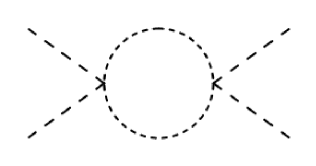
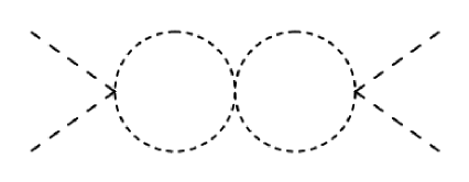
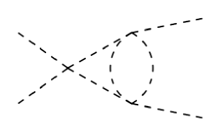
Figure 1: Sample Feynman diagrams that contribute to the beta-functions in $\phi^{4}$ theory. (a) is at one-loop level, (b) and (c) are at two-loop level

The one-loop and two-loop $\beta$-functions are given by,

$$\beta^{\text{1-loop}}(\lambda)=\frac{3\lambda^{2}}{16\pi^{2}}$$ (4)

and

$$\beta^{\text{2-loop}}(\lambda)=\frac{3\lambda^{2}}{16\pi^{2}}-\frac{17}{3}\frac{\lambda^{3}}{(16\pi^{2})^{2}}.$$ (5)

The behaviour of the $\beta$-functions often gives different theoretical limits. One such exciting behaviour is the existence of Fixed points (FPs). Fixed points in RG evolution are regions where the $\beta$-function vanishes and the coupling does not change under scale transformations, indicating scale invariance. The FP is called a Gaussian FP, if $\lambda=0$ (where the theory becomes a free theory); and non-Gaussian, if $\lambda\neq 0$ (corresponds to interacting theories that are scale-invariant). At the one-loop level, the zeros of the beta function can be obtained by setting $\beta^{\text{1-loop}}(\lambda)=0$. This gives the Gaussian Fixed point, $\lambda=0$. At the one-loop level, there are no other Fixed points. However, at the two-loop level, the zeros of the beta function are given by setting $\beta^{\text{2-loop}}(\lambda)=0$.

$$\beta^{\text{2-loop}}(\lambda)=\frac{\lambda^{2}}{16\pi^{2}}\Big{[}3-\frac{17\lambda}{3(16\pi^{2})}\Big{]}=0,$$ (6)

which gives,

$$\lambda=0\ \ \ \ \text{and}\ \ \ \ \ \lambda=\frac{9}{17}(16\pi^{2})\approx 83.60.$$ (7)

Landau pole (LP) is another feature that can be present in an RG evolution. It is the energy scale at which the coupling strength of a quantum field theory becomes infinite. The Landau pole in the one-loop can be obtained by solving the one-loop RG equation. At an LP, the $\lambda(\mu)$ grows without bound at some finite energy scale as can be seen from Equation 9.

$$\mu\frac{d\lambda}{d\mu}=b_{1}\lambda^{2},\ \ \ \implies\ \ \int_{\lambda_{0}}^{\lambda}\frac{d\lambda^{\prime}}{(\lambda^{\prime})^{2}}=\frac{3}{16\pi^{2}}\int_{\mu_{0}}^{\mu}\frac{d(\mu^{\prime})}{\mu^{\prime}},$$ (8)

and finally,

$$\lambda(\mu)=\frac{\lambda_{0}}{1-\frac{3\lambda_{0}}{16\pi^{2}}\ln(\frac{\mu}{\mu_{0}})},$$ (9)

where $\mu_{0}$ is the reference scale and $\lambda_{0}=\lambda(\mu_{0})$. The denominator vanishes at a finite energy scale $\mu=\mu_{0}\exp(\frac{16\pi^{2}}{3\lambda_{0}})$ and hence $\lambda(\mu)$ blows up. The RG evolution of $\lambda$ is shown in Figure 2. In Figure 2(a) for $\lambda=0.5$ at $\mu_{0}=10$ GeV, we do not see any LP or FP at one- and two-loop levels. However, in Figure 2(b) for $\lambda=7$ at $\mu_{0}=10$ GeV we get an LP (shown in the dotted-red curve) at one-loop and an FP at two-loop (solid blue curve). It is evident that the two-loop Fixed point is approaching $\lambda=83.60$, which is independent of the initial values of $\lambda$ for those in which we observe an FP. However, the energy at which the Fixed point behaviour begins will decrease as the initial value of $\lambda$ increases. The detailed analysis of LPs and FPs for $\phi^{4}$ theory, till the seven-loop level has been carried out in six-loop_study_schrock-2016 ; seven-loop_study_schrock-2023 ; six-loop_O(n)_symmetric-2017 and shown that the FPs appearing in $\phi^{4}$-theory are not perturbatively reliable. The non-perturbative analysis of the absence of UV FPs in an $O(N)$ symmetric $\phi^{4}$ theory in four dimensions is described in exact_triviality_no_FP-2009 ; Luscher-Weisz-lattice_phi4 . In this article, we look into the behaviour of scalar quartic coupling at one- and two-loop levels for the inert models, namely inert singlet, inert doublet, and inert triplet.

  

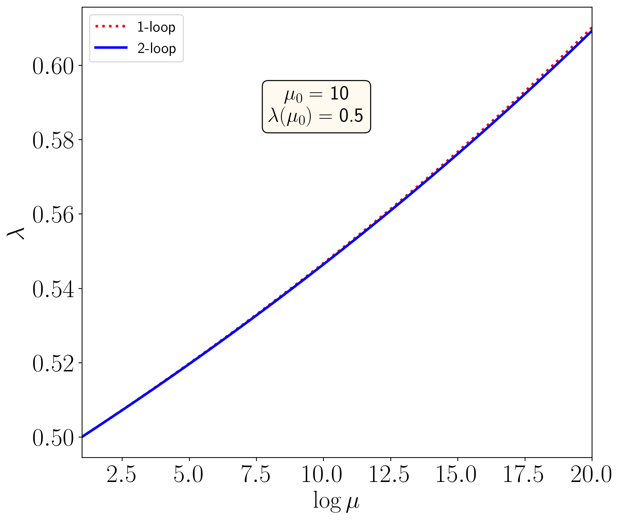
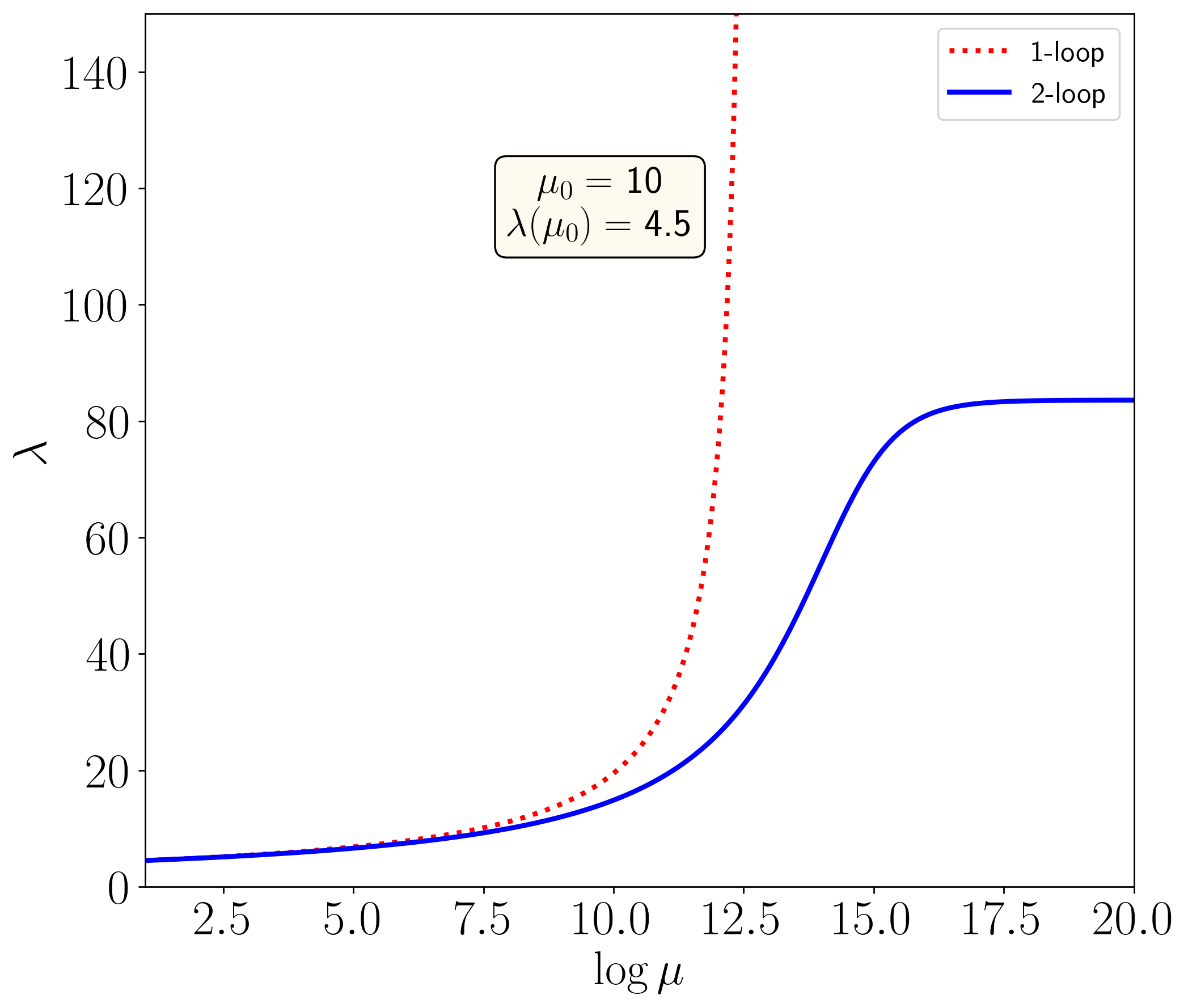
Figure 2: RGE evolution of quartic coupling $\lambda$ in $\phi^{4}$-theory for one- and two-loop orders for (a) the initial value of $\lambda=0.5$ at $\mu=10$ GeV and (b)$\lambda=0.5$ at $\mu=4.5$ GeV, respectively.

3 Absence of Landau poles and Fixed points in the Standard Model

It is obvious that the simplicity of $\phi^{4}$-theory cannot be expected in a highly non-trivial non-abelian gauge theory like the Standard Model, especially where the theory is measured experimentally with high precision at the electroweak(EW) scale. The RG evolution of SM is well-studied focussing on various aspects of the theory. It is worth mentioning that there are no FPs or LPs poles in the RG evolution of parameters in SM, especially the scalar quartic coupling $\lambda$. The one- and two-loop $\beta$-functions of $\lambda$ are functions of itself and other parameters like the Yukawa couplings and gauge couplings. The one-loop $\beta$-function of $\lambda$ is given in Equation 10 and it can be seen that the maximum negative contribution comes from the Yukawa term as depicted in Figure 3(a), which drives $\lambda$ toward the negative values. The corresponding two-loop $\beta$-functions are given in subsection A.1

$$\begin{split}\beta^{\text{SM}}_{\lambda}&=\frac{1}{(4\pi)^{2}}\Bigg{(}\frac{27}{800}g_{1}^{4}+\frac{9}{80}g_{1}^{2}g_{2}^{2}+\frac{9}{32}g_{2}^{4}-\frac{9}{20}g_{1}^{2}\lambda+6\lambda^{2}+3\lambda Y_{t}^{2}-\frac{9}{4}g_{2}^{2}\lambda-\frac{3}{2}Y_{t}^{4}\Bigg{)}\end{split}$$ (10)

  

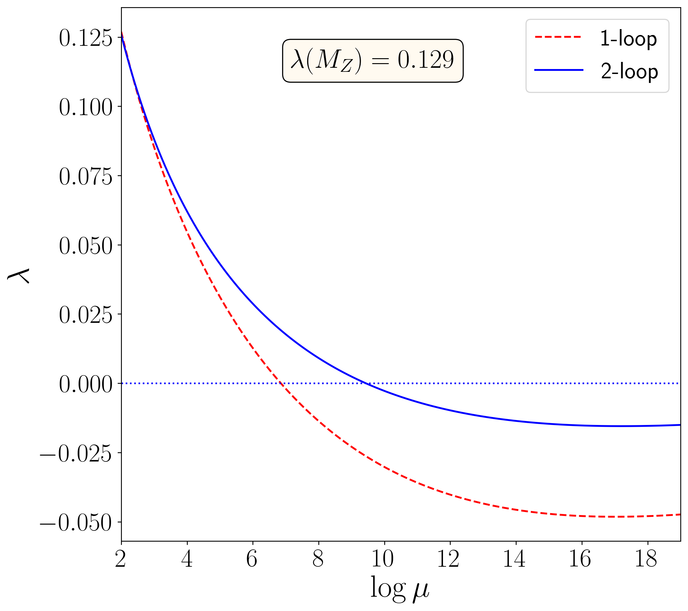
Figure 3: (a) The top-loop diagram contributing negatively to the Higgs quartic coupling. (b) RG evolution of SM quartic coupling $\lambda$ verses scale $\mu$ at one- and two-loop order. The initial value of Higgs-quartic coupling $\lambda_{H}(M_{Z})=0.129$ at tree-level.

Even though these $\beta$-functions are also polynomials, we do not have any freedom in choosing the initial values of the parameters as they are experimentally measured with impeccable precision. With the standard values of the parameters at the electro-weak scale at one-(two-) loop, with $\lambda=$ 0.1271 (0.12604), $g_{1}=$ 0.4639 (0.4626), $g_{2}=$ 0.6476 (0.6478), $g_{3}=$ 1.1666 (1.1666), $Y_{t}=$ 0.9495 (0.9369) while other Yukawa couplings are neglected, the RG evolution of SM Higgs quartic coupling $\lambda$ is shown in Figure 3(b). It can be seen that both in one- and two-loop evolutions we do not have any LP or FP, rather the running coupling $\lambda$ becomes negative at some high energy making the theory unbounded from below and the vacuum unstable. The addition of scalars from different gauge representations can bring back the stability of the electroweak vacuum Jangid:2020qgo ; scalar_shilpa_IDM_tyIIIinvsee-2021 ; scalar_shilpa_IDM_RHN_vac_stab-2020 ; scalar_idm_meta_naj_khan-2015 .

However, when we extend the SM with new fields, additional parameters arise and we may be able to find LP and FP behaviour for some parameter values. In the following sections, we examine a few inert scalar extensions that can exhibit the LP and FP behaviour at one- and two-loop levels, at least for some regions in the parameter space. Along with this observation we also draw bounds from perturbative unitarity anirban-perturbativity-2025 ; carlos-2023 ; chinese-unitary_bounds-2023 ; logan-perturbativity ; Luscher-Weisz-lattice_phi4 ; Ginzburg-perturbativity ; shilpa-anirban-leptoquark at one- and two-loop levels for different initial values of new physics couplings. The evolution of couplings based on the perturbative series expansion of $\beta$-functions will have to satisfy perturbative unitarity at the corresponding energy scales given by

$$\lambda_{i}(\mu)<4\pi,\ \ \ \ \ \ g_{i}<4\pi,\ \ \ \ \ \ Y_{i}<\sqrt{4\pi}.$$ (11)

Here we use the above criteria Equation 11 obtained from the unitarity of scattering cross-sections that are experimentally measurable anirban-perturbativity-2025 ; carlos-2023 ; chinese-unitary_bounds-2023 ; logan-perturbativity ; Luscher-Weisz-lattice_phi4 ; Ginzburg-perturbativity ; shilpa-anirban-leptoquark .

4 Inert Scalar Extensions of the Standard Model

In the following subsections, we study three inert scalar extensions of the Standard Model that give us a number of new parameters, namely the new mass and the quartic couplings. Additional fields and vertices can change the dynamics of the $\beta$-functions and hence affect the behaviour of RG evolution of the couplings including the SM quartic coupling $\lambda$. This leads to the appearance of LPs and FPs at one- and two-loop levels in some parameter regions. The interesting observation is that certain quartic couplings enhance the possibility whereas some others lessen those effects. In this article, we analyse such behaviour for the inert models for three different representations of $SU(2)$, namely, Inert Singlet extension, Inert Doublet extension, and Inert Triplet extension. Moreover, here we are not talking about FPs in the most general sense like in a dynamical system where all the first-order dynamical equations vanish. We are only focussing on the scalar sector and particularly the evolution of the SM-like Higgs quartic coupling $\lambda$. Later we constrain the parameter space of scalar quartic couplings at one- and two-loop using perturbative unitarity anirban-perturbativity-2025 ; carlos-2023 ; chinese-unitary_bounds-2023 ; logan-perturbativity ; Luscher-Weisz-lattice_phi4 ; Ginzburg-perturbativity ; shilpa-anirban-leptoquark as defined in Equation 11.

Figure 4: One-loop Higgs-portal diagram in ISM

4.1 Inert Singlet Model

The simplest scalar extension of the Standard Model (SM) is the inert singlet model (ISM), where the singlet field $S$ does not take part in electroweak symmetry breaking. In this model, an additional complex scalar field $S$ is introduced along with the SM Higgs doublet $\Phi$. The new field $S$ is singlet under SM gauge groups. Additionally, it is odd under a global $\mathbb{Z}_{2}$ symmetry, while the SM particles are even. This $\mathbb{Z}_{2}$ odd nature forbids the $S$ to participate in the EWSB, which is the reason for the term “inert" and also makes it a viable dark matter candidate scalar_DM_Stab_pert_singDM-2010 ; scalar_complx_stab_pheno-2012 ; scalar_EW_vacc_stab-2012 ; scalar_stabilization_EWvac-2012 ; scalar_vac_stab_pert_Z2_Z3_sing_DM-2018 ; singlet-Barger . The scalar potential is given by,

$$V(\Phi,S)=\mu^{2}\Phi^{\dagger}\Phi+m_{S}^{2}S^{*}S+\lambda_{H}(\Phi^{\dagger}\Phi)^{2}+\lambda_{S}(S^{*}S)^{2}+\lambda_{HS}\Phi^{\dagger}\Phi S^{*}S,$$ (12)

where $\Phi=\begin{pmatrix}\phi^{+}&\phi^{0}\end{pmatrix}^{T}$, $S=\frac{1}{\sqrt{2}}(S_{R}+iS_{I})$, $m_{S}$ is the singlet mass, and $\lambda_{H}$ is the SM-like Higgs coupling which is equivalent to $\lambda$ in the SM. $\lambda_{S}$ is the singlet self-coupling and $\lambda_{HS}$ is the Higgs-singlet portal coupling. The corresponding quartic couplings should satisfy the following stability conditions Luigi-1 ; Luigi-2 .

$$\lambda_{H}\geq 0,\ \ \ \ \lambda_{S}\geq 0,\ \ \ \ \lambda_{HS}^{2}-4\lambda_{H}\lambda_{S}>0.$$ (13)

As we are interested in the behaviour of the RG evolution of the quartic couplings, we study their scale dependency by calculating the corresponding $\beta$-functions through SARAH 4.15.1 SARAH_citing-2014 . The complete set of $\beta$-functions for ISM is given in subsection A.2.

We can see a positive contribution proportional to $\lambda^{2}_{HS}$ coming from the one-loop scalar diagram in Figure 4 to the one-loop $\beta$-function given in Equation 14. Some negative contributions can be found at two-loop $\beta$-function proportional to $\lambda_{H}\lambda_{HS}^{2},\,\lambda_{HS}^{3}$ which are suppressed by a loop factor of $\frac{1}{(4\pi)^{4}}$.

$$\begin{split}\beta^{\text{ISM (1-loop)}}_{\lambda_{H}}&=\beta^{\text{SM (1-loop)}}_{\lambda_{H}}+\frac{1}{(4\pi)^{2}}\Bigg{(}\frac{1}{16}\lambda_{HS}^{2}\Bigg{)}\\ \beta^{\text{ISM (2-loop)}}_{\lambda_{H}}&=\beta^{\text{SM}}_{\lambda_{H}}+\frac{1}{(4\pi)^{2}}\Big{(}\frac{1}{16}\lambda_{HS}^{2}\Big{)}-\frac{1}{(4\pi)^{4}}\Big{(}\frac{5}{128}\lambda_{H}\lambda_{HS}^{2}+\frac{1}{64}\lambda_{HS}^{3}\Big{)}.\end{split}$$ (14)

     

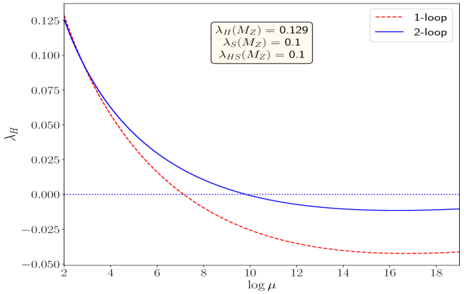
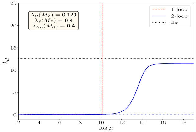
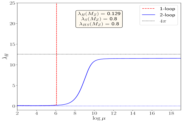
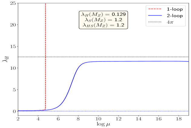
Figure 5: $\lambda_{H}-\log{\mu}$ for ISM at one-loop and two-loop for $\lambda_{HS}(M_{Z})=\lambda_{S}(M_{Z})$ for (a), (b), (c), (d) plots are $0.1$, $0.4$, $0.8$, $1.2$, respectively. with $\lambda_{H}(M_{Z})=0.129$ for all cases.

The evolution of SM-like Higgs quartic coupling $\lambda_{H}$ in the ISM is shown in Figure 5. Here $\lambda_{H}$ varies with respect to the energy scale $\mu$ (more precisely with respect to $t=\log\mu$). Different sub-figures correspond to different initial values of the other quartic couplings $\lambda_{HS}$ and $\lambda_{S}$. However, in every case, $\lambda_{H}$ is fixed to $0.129$ at the electroweak scale ($M_{Z}$), i.e., $\lambda_{H}$ = 0.1271 at one-loop and 0.12604 at two-loops. The one(two)-loop $\beta$-functions are shown by the dotted red (solid blue) curves. Figure 5(a) represents the variation of $\lambda_{H}$ for the initial values of $\lambda_{S}=\lambda_{{HS}}=0.1$ and for both one- and two-loop, the $\lambda_{H}$ becomes negative at certain scales, similar to the SM as depicted in Figure 3. However, as we increase the new coupling values to $\lambda_{S}=\lambda_{{HS}}=0.4$ in Figure 5(b), we observe an interesting behaviour. For one-loop, the evolution of $\lambda_{H}$ hits a Landau pole at $\mu\approx 10^{10}$ GeV, whereas, for two-loop, we see that $\lambda_{H}$ attains a Fixed point around $\mu\approx 10^{15}$ GeV. As we move to Figure 5(c) for $\lambda_{S}=\lambda_{{HS}}=0.8$, the behaviour of LP at one-loop and FP at two-loop appear much earlier, around $\mu\approx 10^{6},10^{10}$ GeV, respectively. Similarly, for $\lambda_{S}=\lambda_{{HS}}=1.2$, the behaviour of such LP and FP appear further earlier, around $\mu\approx 10^{5},^{9}$ GeV, respectively, as shown in Figure 5(d). The observation of such one-loop LPs and two-loop FPs in ISM is similar to $\phi^{4}$ theory as described in section 2.

     

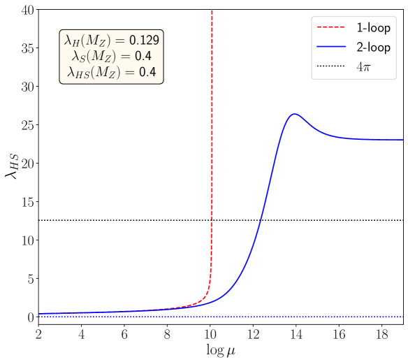
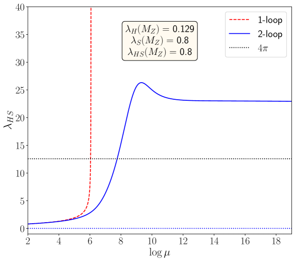
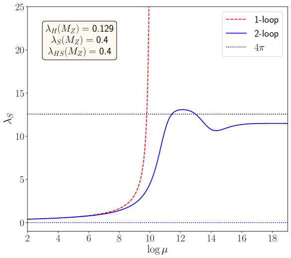
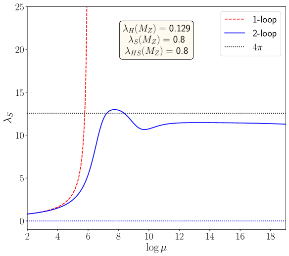
Figure 6: $\lambda_{HS}-\log{\mu}$ in (a), (b) and $\lambda_{S}-\log{\mu}$ in (c), (d ) are depicted for ISM at one-loop and two-loop for $\lambda_{H}(M_{Z})=0.129$. $\lambda_{HS}(M_{Z})=\lambda_{S}(M_{Z})=0.4,\,0.8$ are fixed for (a), (c) and (b), (d), respectively.

Figure 6 shows the behaviour of the RG evolution of $\lambda_{S}$ and $\lambda_{{HS}}$ where similar observations are found. Figure 6(a), (c) represent the evolution of $\lambda_{S}$ and $\lambda_{HS}$ with the initial values $\lambda_{S}(M_{Z})=$ $\lambda_{HS}(M_{Z})=0.4$ where the one-loop LP (two-loop FP) are seen at the scales around $10^{10}(10^{16})$ GeV respectively. In Figure 6(b), (d) for $\lambda_{S}(M_{Z}),\ \lambda_{HS}(M_{Z})=0.8$ we see such LP(FP) at the scales around $10^{5}(10^{9})$ GeV. For larger initial values of $\lambda_{S}(M_{Z}),\lambda_{HS}(M_{Z})$ the LP(FP) are achieved at much relatively lower energy scales. Even though FP appears $\lesssim 4\pi$ for $\lambda_{S}$, for $\lambda_{{HS}}$, it crosses $4\pi$.

Thus, higher initial values of new physics couplings i.e., $\lambda_{S},\lambda_{{HS}}$ promote LPs and FPs for one- and two-loop levels, respectively. For convenience, we define $\alpha=\frac{\lambda_{HS}(M_{Z})}{\lambda_{S}(M_{Z})}$, which gives the relative strength of $\Phi^{\dagger}\Phi S^{*}S$ term over $(S^{*}S)^{2}$ term. Figure 7 gives the values of $\lambda_{S}$ and $\alpha$ for which there is an FP in the evolution of $\lambda_{H}(\mu)$ at the two-loop level. The colour code gives the energy scale at which the FP begins. The colour of the points, as shown in the figure, varies from blue($10^{8}$ GeV) to yellow ($10^{19}$ GeV). It is evident that for lower initial values of $\lambda_{S}$, the FPs occur for higher values of $\alpha$. One can see that for $\lambda_{S}<1$ the FPs appear around $\mu>10^{18}$ GeV, and for $\lambda_{S}>1.0$ the FPs appear around $\mu>10^{8-12}$ GeV. But for very high values of $\lambda_{S}$ and $\lambda_{HS}$, the FP behaviour is absent. In a nutshell, an increase in $\alpha$ promotes FP, provided $\lambda_{S}$ is small.

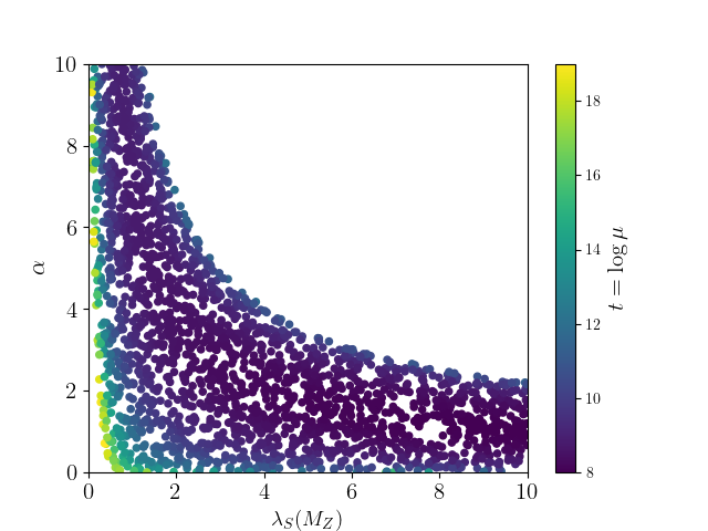
Figure 7: Occurrence of FP at two-loop level for different initial values of $\alpha=\frac{\lambda_{HS}(M_{Z})}{\lambda_{S}(M_{Z})}$ and $\lambda_{S}(M_{Z})$. Initial value of $\lambda_{H}(M_{Z})=0.129$ for all the points.

Figure 8: Type of scalar four-point vertices in Inert Singlet Model

If we expand the ISM potential as shown in Equation 15 and Equation 16, we find them as functions of modulus filed terms, without any residual phases, very similar to $\phi^{4}$ theory in Equation 1. The LP and FP for odd- and even loops are also seen in $\phi^{4}$ theory six-loop_study_schrock-2016 ; seven-loop_study_schrock-2023 . These interactions are represented by the tree-level diagrams of the type shown in Figure 8, where $\phi^{a}$, $\phi^{b}$ $=$ $\phi^{+}$, $\phi^{0}$, $S$.

$$\lambda_{HS}(\Phi^{\dagger}\Phi\ S^{*}S)+\lambda_{S}(S^{*}S)^{2}=\lambda_{HS}(\left|\phi_{0}\right|^{2}|S|^{2}+\left|\phi^{+}\right|^{2}|S|^{2})+\lambda_{S}|S|^{4},$$ (15)

$$\lambda_{H}(\Phi^{\dagger}\Phi)^{2}=\lambda_{H}(|\phi^{0}|^{4}+2|\phi^{0}|^{2}|\phi^{+}|^{2}+|\phi^{+}|^{4}).$$ (16)

This seems to be encouraging the appearance of the FPs, as seen in $\phi^{4}$ theory also. However, the role of the residual phases in spoiling this FP behaviour is prominent in the case of IDM, which is discussed in subsection 4.3.

In Figure 9 we plot the one- and two-loop perturbativity limits of $4\pi$ as given in Equation 11 on the $\lambda_{S}(M_{Z})-\lambda_{HS}(M_{Z})$ plane considering the bounds from perturbative unitarity anirban-perturbativity-2025 ; carlos-2023 ; chinese-unitary_bounds-2023 ; logan-perturbativity ; Luscher-Weisz-lattice_phi4 ; Ginzburg-perturbativity ; shilpa-anirban-leptoquark . Different colour codes correspond to different perturbativity scales starting from $10^{2}-10^{19}$ GeV. Generically, the lower the couplings higher the perturbativity scales. At one-loop for the coupling constants $\lambda_{S}(M_{Z})\lesssim 0.2$ and $\lambda_{HS}(M_{Z})\lesssim 0.5$, the whole parameter space is perturbative till the Planck scale which is similar even at the two-loop level. However, for larger values of these couplings, the perturbative limits go down to lower scales and the two-loop limits also differ from one-loop. The one-loop perturbativity limits as shown in Figure 9(a), when $\lambda_{S}(M_{Z})>1.5$, regardless of the value of $\lambda_{HS}$, perturbativity hits at energy scales between $10^{2}-10^{3}$ GeV. For relatively higher values of $\lambda_{HS}(M_{Z})>2.0$, relatively lower values of $\lambda_{S}$ hit the perturbativity limit for the scale $10^{2}-10^{3}$ GeV. When $1.0<\lambda_{HS}<1.5$, the perturbativity hits around $10^{3}-10^{4}$ GeV. For the two-loop, the perturbative limit as shown in Figure 9(b), gets relaxed and larger values of quartic couplings are now allowed. For $\lambda_{S}(M_{Z})>3.0$, it hits the perturbativity for the scale $10^{2}-10^{3}$ GeV. For larger values of $\lambda_{HS}(M_{Z})>2.8$, the perturbativity hits at a similar scale for lower $\lambda_{S}(M_{Z})$. The yellow colour region inside the black contour shows the unstable points that fail to satisfy the bounded-from-below stability conditions in Equation 13. For multi-TeV dark matter, where these parameter regions are allowed by dark matter, these theoretical constraints are more relevantBandyopadhyay:2024plc ; Bandyopadhyay:2023joz ; Katayose:2021mew .

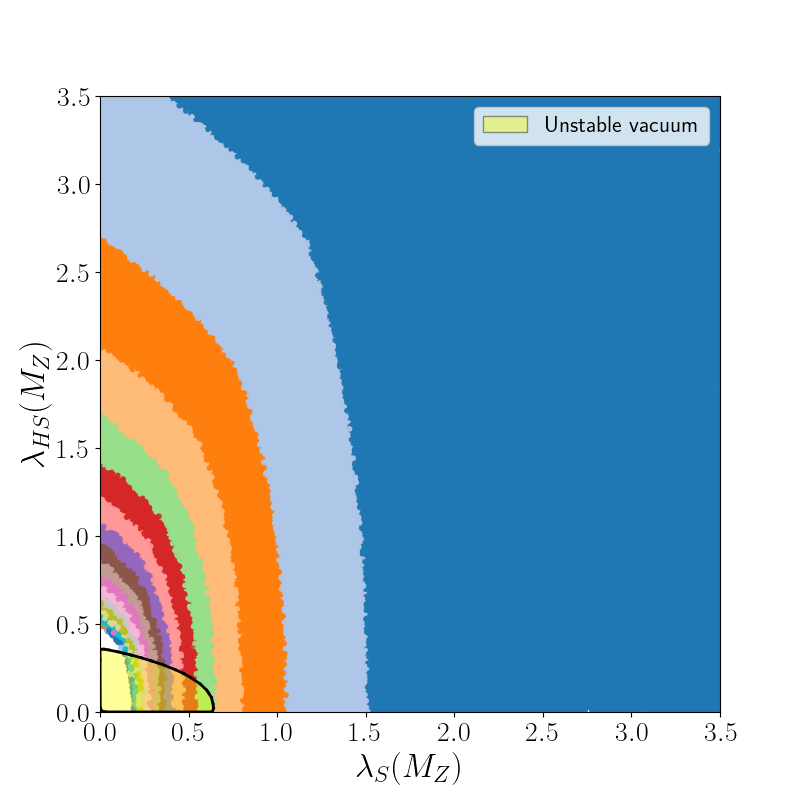
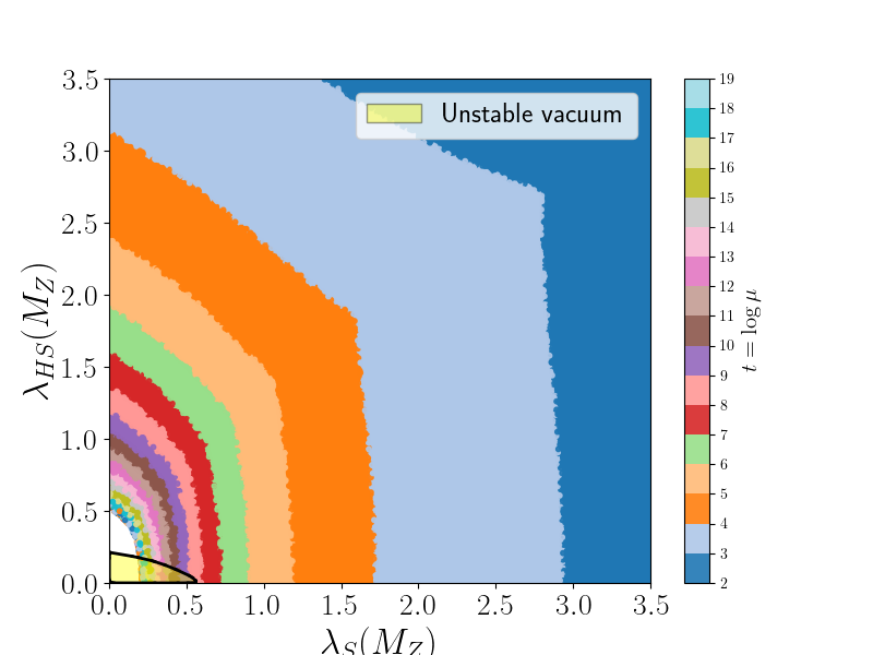
Figure 9: Perturbativity limit of one-loop and two-loop RGE evolution in Inert Singlet Model. Initial value of Higgs-self quartic coupling $\lambda_{H}(M_{Z})=0.129$ for all cases. $\lambda_{S}(M_{Z})$ is along the x-axis and $\lambda_{HS}(M_{Z})$ is along the y-axis.

4.2 Inert Triplet Model

The Inert triplet model (ITM) consists of an $SU(2)_{L}$ triplet scalar $T$ with zero hypercharge ($Y=0$) along with the SM Higgs doublet. The triplet as given in Equation 17 is odd under a $\mathbb{Z}_{2}$ symmetry and thus does not play any role in EWSB, therefore it is called “inert". The neutral component provides a real scalar dark matter.

$$\Phi=\begin{pmatrix}\phi^{+}\\ \phi^{0}\end{pmatrix}\ \ \ \ \ \text{and}\ \ \ \ \ \ T=\frac{1}{2}\begin{pmatrix}T^{0}&\sqrt{2}T^{+}\\ \sqrt{2}T^{-}&-T^{0}\end{pmatrix}.$$ (17)

The triplet field is odd under $\mathbb{Z}_{2}$ symmetry while all the SM fields are even under $\mathbb{Z}_{2}$. The covariant derivative for the triplet is given by,

$$D_{\mu}T=\partial_{\mu}T-ig_{2}\commutator{\frac{\sigma^{a}}{2}W^{a}_{\mu}}{T},$$ (18)

while the scalar potential is as follows:

$$\begin{split}V=m_{H}^{2}\Phi^{\dagger}\Phi+m_{T}^{2}\ \text{Tr}[T^{\dagger}T]+\lambda_{H}(\Phi^{\dagger}\Phi)^{2}+\lambda_{T}\ (\text{Tr}[T^{\dagger}T])^{2}+\lambda_{HT}(\Phi^{\dagger}\Phi)\text{Tr}[T^{\dagger}T],\end{split}$$ (19)

where $\lambda_{H}$ is the SM-like Higgs self-coupling, $\lambda_{T}$ is the triplet self-coupling and $\lambda_{{HT}}$ is the Higgs-triplet portal coupling. For a stable vacuum, the quartic coupling must satisfy the following stability conditions Jangid:2020qgo ; Bandyopadhyay:2024plc

$$\lambda_{H}\geq 0,\ \ \ \ \lambda_{T}\geq 0,\ \ \ \ \lambda_{HT}^{2}-4\lambda_{H}\lambda_{T}\geq 0.$$ (20)

The $\beta$-function of SM-like Higgs quartic coupling generated using SARAH 4.15.1SARAH_citing-2014 is given, at the one-loop level, in Equation 21 and the rest of the $\beta$-functions in two-loop are given in Appendix A.3. Even though the potential and new physics couplings look similar to ISM, the $\beta$-function looks very different from the $\beta^{\text{ISM}}_{\lambda_{H}}$ in the case of ISM (Equation 14) since the triplet is in a non-trivial representation of $SU(2)$ that involves the gauge coupling $g_{2}$.

$$\begin{split}\beta^{\text{ITM}}_{\lambda_{H}}=\beta^{\text{SM}}_{\lambda_{H}}+\frac{1}{(4\pi)^{2}}&\Big{(}\frac{3}{2}\lambda_{HT}^{2}\Big{)}+\frac{1}{(4\pi)^{4}}\Big{(}\frac{11}{2}g_{2}^{4}\lambda_{H}+\frac{5}{4}g_{2}^{4}\lambda_{HT}+\frac{9}{2}g_{2}^{2}\lambda_{HT}^{2}\\ &-15\lambda_{H}\lambda_{HT}^{2}-2\lambda_{HT}^{3}-\frac{7}{20}g_{1}^{2}g_{2}^{4}-\frac{7}{4}g_{2}^{6}\Big{)}.\end{split}$$ (21)

The evolution of SM-like Higgs quartic coupling $\lambda_{H}$ is shown in Figure 10. Different figures correspond to different initial values of the other quartic couplings, say $\lambda_{T}$ and $\lambda_{HT}$ where the initial value of $\lambda_{H}(M_{Z})=0.129$ at the electro-weak scale. Figure 10(a) shows the variation of $\lambda_{H}$ for lower initial values of $\lambda_{{HT}}(M_{Z})=\lambda_{T}(M_{Z})=0.1$. The results look similar to SM and ISM as both one(two)-loop $\lambda_{H}$ go negative at certain scales. As we increase $\lambda_{{HT}}(M_{Z})=\lambda_{T}(M_{Z})=0.4$ in Figure 10(b), $\lambda_{H}$ becomes non-zero till the Planck scale for both one(two)-loop $\beta_{\lambda_{H}}$. However, unlike Figure 5(b), here we do not get any Landau poles at one-loop or Fixed points at two-loop for $\lambda_{{HT}}(M_{Z})=\lambda_{T}(M_{Z})=0.4$.

    

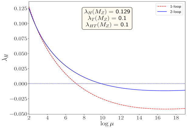
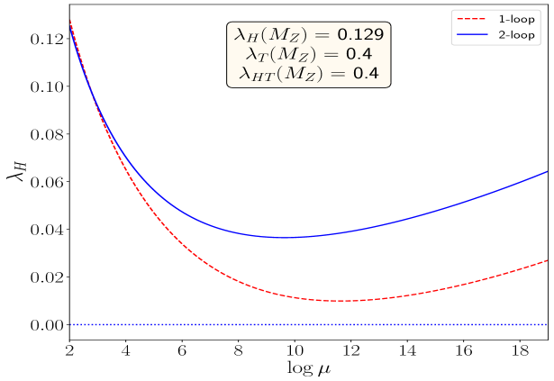
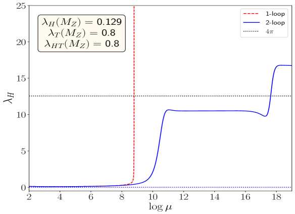
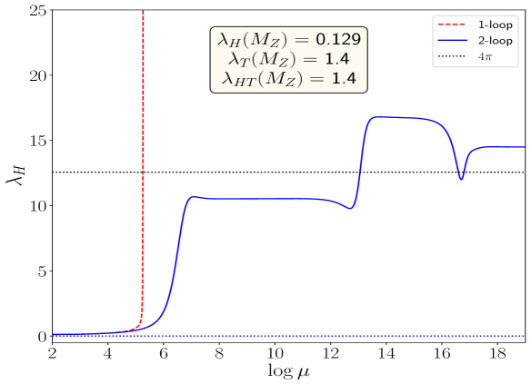
Figure 10: One-loop and Two-loop RGE evolution of SM Higgs-like quartic coupling in Inert Triplet Model. Initial value of $\lambda_{H}(M_{Z})=0.129$ for all cases. Initial values of $\lambda_{HT}(M_{Z})$ and $\lambda_{T}(M_{Z})$ for (a), (b), (c), (d) plots are $0.1$, $0.4$, $0.8$, $1.4$, respectively.

From Figure 10(c) it is clear that there is an FP behaviour in the two-loop evolution of $\lambda_{H}$ (solid blue curve) for the initial value of $\lambda_{{HT}}(M_{Z})=\lambda_{T}(M_{Z})=0.8$. We get a Landau pole in the one-loop evolution (dotted red curve). Similar behaviour can be found in Figure 10(d) for the initial value of $\lambda_{{HT}}(M_{Z})=\lambda_{T}(M_{Z})=1.2$ also. , Similar to the case of ISM, the higher initial values will lead to attaining the LP and FP at relatively lower energy scales. However, we notice the appearance of two different Fixed points for two different values of $\lambda_{H}$, one below $4\pi$ and one above $4\pi$, which was absent in $\phi^{4}$ theory and ISM.

 

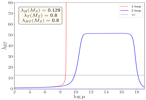
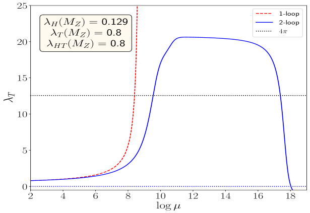
Figure 11: $\lambda_{HT}-\log{\mu}$ in (a), and $\lambda_{T}-\log{\mu}$ in (b) are depicted for ITM at one-loop and two-loop for $\lambda_{H}(M_{Z})=0.129$, $\lambda_{HT}(M_{Z})=\lambda_{T}(M_{Z})=0.8$.

To complete the analysis of scalar quartic couplings we also see the evolution of $\lambda_{T}$ and $\lambda_{HT}$ verses the scale in Figure 11(a) and (b) respectively for the initial values of $\lambda_{T}(M_{Z})=\lambda_{HT}(M_{Z})=0.8$. Though we notice FP behaviour in both the cases, however they appear above $4\pi$ in the coupling constant values. Though the appearance of the FP happens in the scale $\sim 10^{10}$ GeV, similar to $\lambda_{H}$, around $\mu\mathrel{\mathop{\kern 0.0pt\hbox to0.0pt{\raise 0.86108pt\hbox{$>$}\hss}}\lower 3.87495pt\hbox{\kern-1.90002pt$\sim$}}10^{18}$ GeV, we see a dip in the couplings that go beyond zero.

One could obtain the parameter ranges where FP is occurring for different initial values of $\lambda_{T}(M_{Z})$ and $\lambda_{HT}(M_{Z})$ for a fixed value of $\lambda_{H}(M_{Z})$. For convenience, we define $\alpha=\frac{\lambda_{HT}(M_{Z})}{\lambda_{S}(M_{Z})}$, which gives us the relative strength of $\Phi^{\dagger}\Phi S^{*}S$ term over $[Tr(T^{\dagger}T)]^{2}$ term.

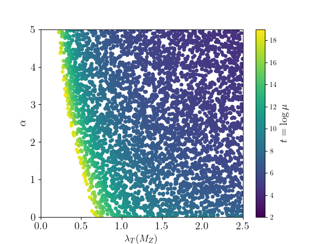
Figure 12: Occurrence of two-loop FP for different initial values of $\alpha=\frac{\lambda_{HT}(M_{Z})}{\lambda_{T}(M_{Z})}$ and $\lambda_{T}(M_{Z})$. Initial value of $\lambda_{H}(M_{Z})=0.129$ for all points.

Figure 12 gives the values of $\lambda_{T}(M_{Z})$ and $\alpha$ for which there are two-loop FPs in the evolution of $\lambda_{H}(\mu)$. The colour code gives the energy scale at which the FP begins. For lower initial values of $\lambda_{T}(M_{Z})$, the FP occurs when the $\alpha$ value is higher. As initial values of $\lambda_{T}(M_{Z})$ and $\alpha$ become higher, the FP occurs at a lower energy scale. But for very high values of $\lambda_{T}(M_{Z})$ and $\lambda_{HT}(M_{Z})$, the FP behaviour is absent. In conclusion, the increase in the $\alpha$ promotes the FP, provided $\lambda_{T}(M_{Z})$ is small as in the case of ISM.

As we discussed in the case of the ISM, we like to see if the scalar potential depends only on the modulus-squared terms and not on the phases of the complex fields. The $\lambda_{H}$ term is given by,

$$\lambda_{H}(\Phi^{\dagger}\Phi)^{2}=\lambda_{H}\big{(}\left|\phi^{0}\right|^{4}+2\left|\phi^{0}\right|^{2}\left|\phi^{+}\right|^{2}+\left|\phi^{+}\right|^{4}\big{)}.$$ (22)

The $\lambda_{T}$ term is given by,

$$\begin{split}\lambda_{T}(\Tr(T^{\dagger}T))^{2}=&\lambda_{T}\Big{(}\frac{1}{4}\left|T^{0}\right|^{4}+\frac{1}{2}\left|T^{0}\right|^{2}\left|T^{-}\right|^{2}+\frac{1}{4}\left|T^{-}\right|^{4}\\ &+\frac{1}{2}\left|T^{0}\right|^{2}\left|T^{+}\right|^{2}+\frac{1}{2}\left|T^{-}\right|^{2}\left|T^{+}\right|^{2}+\frac{1}{4}\left|T^{+}\right|^{4}\Big{)}.\end{split}$$ (23)

The $\lambda_{HT}$ term is given by,

$$\begin{split}\lambda_{HT}(\Phi^{\dagger}\Phi)\Tr(T^{\dagger}T)=\ \frac{1}{2}\lambda_{HT}\Big{(}&\left|T^{0}\right|^{2}\left|\phi^{0}\right|^{2}+\left|T^{-}\right|^{2}\left|\phi^{0}\right|^{2}+\left|T^{+}\right|^{2}\left|\phi^{0}\right|^{2}\\ &+\left|T^{0}\right|^{2}\left|\phi^{+}\right|^{2}+\left|T^{-}\right|^{2}\left|\phi^{+}\right|^{2}+\left|T^{+}\right|^{2}\left|\phi^{+}\right|^{2}\Big{)}.\end{split}$$ (24)

Like in the case of ISM, all the terms in the scalar potential depend only on the absolute values of the fields and not on the residual phases. Later in section subsection 4.3, we will illustrate that these are the kind of terms that favour a two-loop FP behaviour.

Figure 13 presents the perturbative limit of $4\pi$ at one- and two-loop on the $\lambda_{T}(M_{Z})-\lambda_{HT}(M_{Z})$ plane for different scales similar to Figure 9. Planck scale perturbativity at one-loop can be achieved till $\lambda_{T}(M_{Z})\lesssim 0.5,\,\lambda_{HT}(M_{Z})\lesssim 0.4$, and further increment of $\lambda_{HT}(M_{Z})$ lowers the perturbative scale. For two-loop, a similar observation is made for $\lambda_{T}(M_{Z})\lesssim 0.6,\,\lambda_{HT}(M_{Z})\lesssim 0.4$. For higher values of couplings, the perturbativity scales decrease further and the two-loop limits differ more from the one-loop. In Figure 13(a), at the one-loop level, we see that for $\lambda_{T}(M_{Z})>2.0$ the perturbativity scale appears at $10^{2-3}$ GeV. As we increase the $\lambda_{HT}(M_{Z})$ the perturbative limit happens for even lower values of $\lambda_{T}(M_{Z})$ at the same scale. For two-loop as described in Figure 13(b), when $\lambda_{T}(M_{Z})>2.6$ the perturbativity scale appears at $10^{2-3}$ GeV As we increase the $\lambda_{HT}(M_{Z})$ further the allowed values of $\lambda_{T}(M_{Z})$ reduce further for the same scale. Overall the two-loop results are more relaxed as compared to one-loop, similar to the inert singlet case. Black-contoured yellow regions correspond to an unstable vacuum which fails to satisfy Equation 20. Generically, this happens for lower values of the quartic couplings.

  

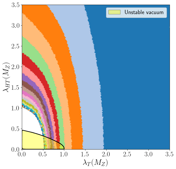
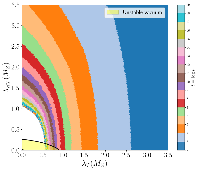
Figure 13: Perturbativity limit of one-loop and two-loop RGE evolution in Inert Triplet Model. Initial value of Higgs-self quartic coupling $\lambda_{H}(M_{Z})=0.129$ for all cases. $\lambda_{T}(M_{Z})$ is along the x-axis and $\lambda_{HT}(M_{Z})$ is along the y-axis.

4.3 Inert Doublet Model

In the inert doublet model (IDM), the SM Higgs sector is augmented with another $SU(2)_{L}$ doublet ($\Phi_{2}$) that has the same hypercharge as the SM Higgs field ($\Phi_{1}$), $Y=\frac{1}{2}$. This doublet is odd under $\mathbb{Z}_{2}$ symmetry while all the SM fields are even scalar_2hdm_review-2012 ; scalar_2hdm_stab_tree_CPV-2004 ; scalar_2hdm_gen_sym_break_stab-2006 ; scalar_idm_DM_archetype-2007 ; scalar_idm_meta_naj_khan-2015 ; scalar_idm_tree_stab_new_constraints-2017 ; scalar_idm_vac_stab-2018 ; Luigi-3 ; Jangid:2020qgo . The scalar potential of the IDM is written as,

$$\begin{split}V(\Phi_{1},\Phi_{2})=&m_{11}^{2}\Phi_{1}^{\dagger}\Phi_{1}+m_{22}^{2}\Phi_{2}^{\dagger}\Phi_{2}+\lambda_{1}(\Phi_{1}^{\dagger}\Phi_{1})^{2}+\lambda_{2}(\Phi_{2}^{\dagger}\Phi_{2})^{2}+\lambda_{3}(\Phi_{1}^{\dagger}\Phi_{1})(\Phi_{2}^{\dagger}\Phi_{2})\\ &+\lambda_{4}(\Phi_{1}^{\dagger}\Phi_{2})(\Phi_{2}^{\dagger}\Phi_{1})+\lambda_{5}((\Phi_{1}^{\dagger}\Phi_{2})^{2}+\text{ h.c.}),\end{split}$$ (25)

where $\Phi_{1}=\begin{pmatrix}\phi_{1}^{+}&\phi_{1}^{0}\end{pmatrix}^{T}$ and $\Phi_{2}=\begin{pmatrix}\phi_{2}^{+}&\phi_{2}^{0}\end{pmatrix}^{T}$. The field $\Phi_{2}$ is called “inert" because it does not take part in EWSB. The coefficients $m^{2}_{11}$ and $m^{2}_{22}$ are the mass terms, $\lambda_{1}$ is the SM-like Higgs self-coupling (which is equivalent to $\lambda_{H}$ in ISM and ITM), $\lambda_{2}$ is the inert doublet self-coupling, and $\lambda_{3,4,5}$ are the different portal couplings. The stability conditions for this potential are the followingJangid:2020qgo ; scalar_2hdm_review-2012 ; Eriksson:2009ws

$$\lambda_{1}\geq 0,\ \ \ \ \lambda_{2}\geq 0,\ \ \ \ \lambda_{3}\geq-2\sqrt{\lambda_{1}\lambda_{2}},\ \ \ \ \lambda_{3}+\lambda_{4}-2|\lambda_{5}|\geq-2\sqrt{\lambda_{1}\lambda_{2}}.$$ (26)

The $\beta$-functions for this model are also obtained using SARAH 4.15.1. The $\beta_{\lambda_{1}}$ at one-loop is shown in Equation 27 and the complete set of two-loop $\beta$-functions are given in Appendix A.4.

$$\beta^{\text{IDM}}_{\lambda_{1}}=\beta^{\text{SM}}_{\lambda_{1}}+\frac{1}{(4\pi)^{2}}\Big{(}2\lambda_{3}^{2}+2\lambda_{3}\lambda_{4}+\lambda_{4}^{2}+4\lambda_{5}^{2}\Big{)}$$ (27)

The evolutions of SM-like Higgs quartic coupling $\lambda_{1}$ in the inert doublet scenario, for different initial values of the other quartic couplings $\lambda_{i\neq 1}$, are shown in Figure 14. Like in the cases of ISM and ITM, the one-loop evolution is shown in the red dashed curve and the two-loop evolution is the blue solid curve. Similar to the previous case, we take $\lambda_{H}(M_{Z})=0.129$ and other quartic couplings are varied as $\lambda_{i\neq 1}(M_{Z})=0.01,\,0.4,\,0.8$, and $1.2$ for Figure 14(a), Figure 14(b), Figure 14(c) and Figure 14(d), respectively. We can see from Figure 14(a) that $\lambda_{1}=\lambda_{H}$ becomes negative for both one(two)-loop as in SM. However, it is worth mentioning that when we increase $\lambda_{i\neq 1}(M_{Z})=0.1$, the one-loop will remain negative at higher scales but in the two-loop, it remains positive till the Planck scale. When we increase the new physics couplings $\lambda_{i\neq 1}(M_{Z})=0.4$, $\lambda_{1}$ hits LP at $\mu\approx 10^{7.5}(10^{8.7})$ GeV for one(two)-loop $\beta$-functions, respectively. The behaviour is similar for higher values of $\lambda_{i\neq 1}$ i.e., $\lambda_{i\neq 1}(M_{Z})=0.8$ where the LPs appear much earlier $\mu\approx 10^{4.7}(10^{5.7})$ GeV for one(two)-loop $\beta$-functions, respectively as can be seen from Figure 14(c). Finally, in Figure 14(d) we plot for $\lambda_{i\neq 1}(M_{Z})=1.2$ where the LPs come around $\mu\approx 10^{3.6}(10^{4.5})$ GeV for one(two)-loop $\beta$-functions, respectively. Even though we do not find any FPs for higher values of $\lambda_{i\neq 1}$, unlike SM or ISM, the situation is far more interesting as we elaborate in the following paragraphs.

    

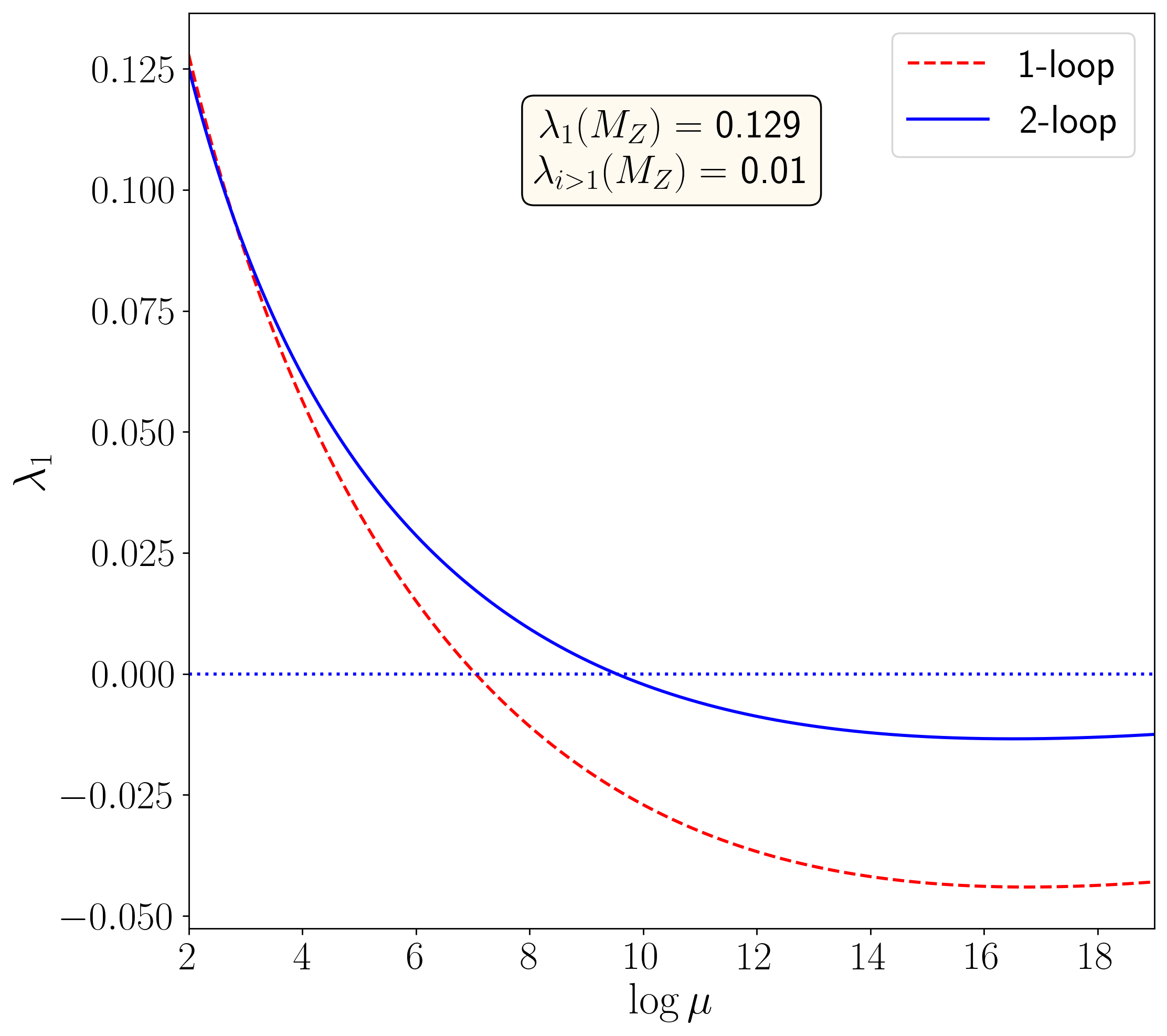
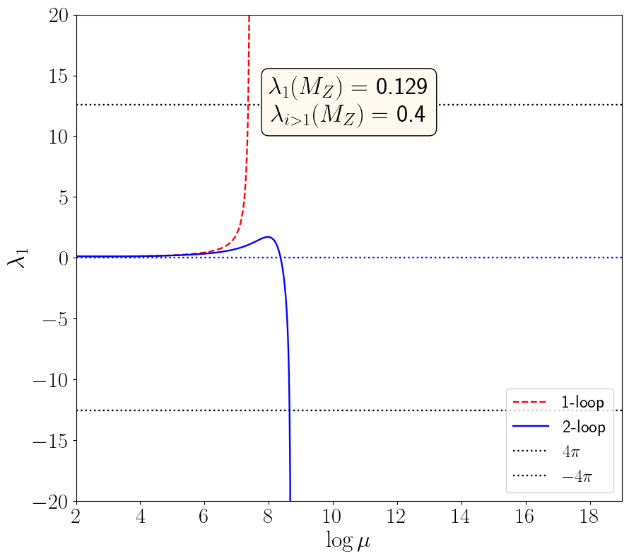
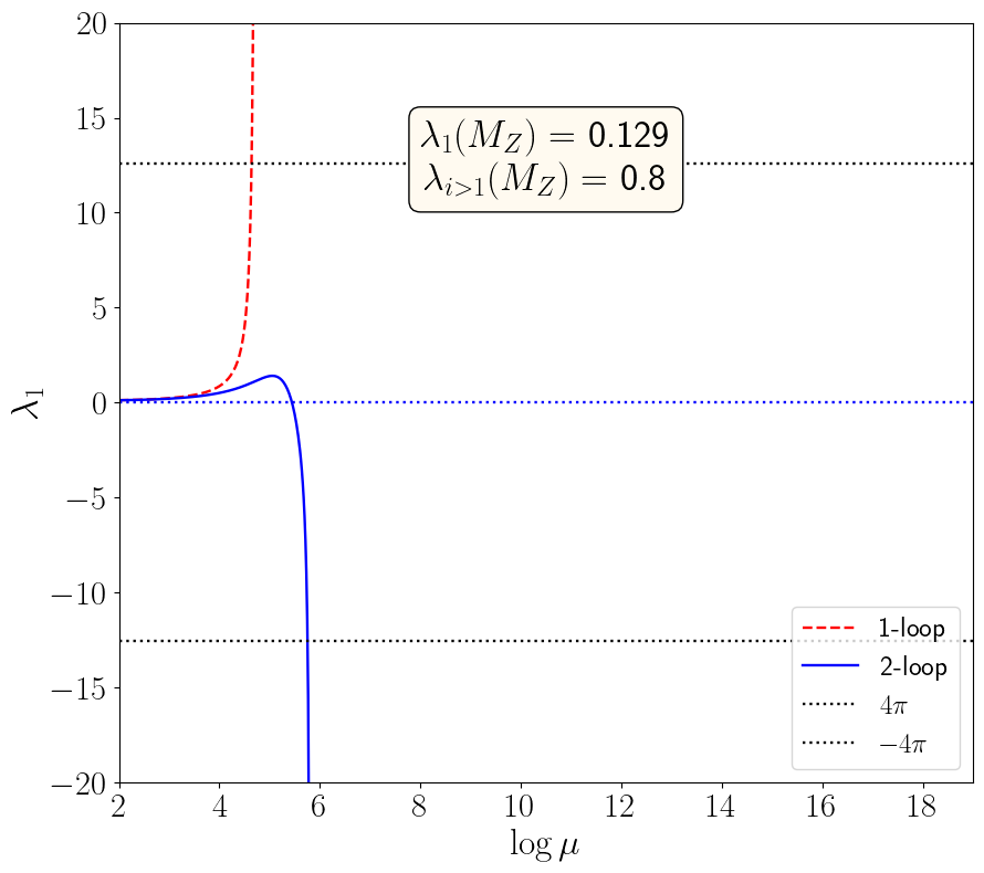
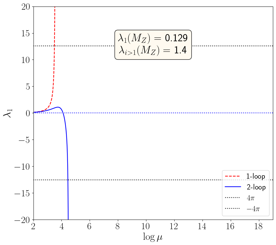
Figure 14: Two-loop RGE evolution of SM Higgs-like quartic coupling in Inert Doublet Model. The initial value of $\lambda_{i\neq 1}(M_{Z})$ for (a), (b), (c), (d) plots are $0.01,0.4,0.8,1.4$, respectively. Initial value of Higgs-self quartic coupling $\lambda_{1}(M_{Z})=0.129$ for all cases.

Non-appearance of the FP in the case of IDM can be explained if we analyse the portal couplings in detail, as we did for ISM and ITM in subsection 4.1 and subsection 4.2, respectively. It can be seen from subsection 4.3, that $\lambda_{1,2,3}$-terms are terms that do not contain any residual phases. They are similar to the terms obtained for ISM in Equation 15, Equation 16, and for ITM in Equation 23 and Equation 24 in the sense that they only depend on the square of the absolute values of the fields.

$$\lambda_{1}(\Phi_{1}^{\dagger}\Phi_{1})^{2} = \lambda_{1}(|\phi_{1}^{0}|^{4}+2|\phi_{1}^{0}|^{2}|\phi_{1}^{+}|^{2}+|\phi_{1}^{+}|^{4}),$$

$$\lambda_{2}(\Phi_{2}^{\dagger}\Phi_{2})^{2} = \lambda_{2}(|\phi_{2}^{0}|^{4}+2|\phi_{2}^{0}|^{2}|\phi_{2}^{+}|^{2}+|\phi_{2}^{+}|^{4}),$$

$$\lambda_{3}(\Phi_{1}^{\dagger}\Phi_{1})(\Phi_{2}^{\dagger}\Phi_{2}) = \lambda_{3}(|\phi_{1}^{0}|^{2}|\phi_{2}^{0}|^{2}+|\phi_{1}^{+}|^{2}|\phi_{2}^{0}|^{2}+|\phi_{1}^{0}|^{2}|\phi_{2}^{+}|^{2}+|\phi_{1}^{+}|^{2}|\phi_{2}^{+}|^{2}).$$ (28)

However, if we expand the $\lambda_{4,5}$ terms, as given in Equation 29 and Equation 30, we can see that they not only depend on the modulus of the terms but also depend on the residual phases.

$$\lambda_{4}(\Phi_{1}^{\dagger}\Phi_{2})(\Phi_{2}^{\dagger}\Phi_{1})=\lambda_{4}(|\phi_{1}^{0}|^{2}|\phi_{2}^{0}|^{2}+\phi_{1}^{0}\phi_{2}^{+}\phi_{1}^{+*}\phi_{2}^{0*}+\phi_{1}^{+}\phi_{2}^{0}\phi_{1}^{0*}\phi_{2}^{+*}+|\phi_{1}^{+}|^{2}|\phi_{2}^{+}|^{2}),$$ (29)

$$\begin{split}\lambda_{5}((\Phi_{1}^{\dagger}\Phi_{2})^{2}+\text{ h.c.})=&\ \lambda_{5}(\phi_{2}^{0}{}^{2}\phi_{1}^{0*}{}^{2}+2\phi_{2}^{0}\phi_{2}^{+}\phi_{1}^{0*}\phi_{1}^{+*}+\phi_{2}^{+}{}^{2}\phi_{1}^{+*}{}^{2}\\ &+\phi_{1}^{0}{}^{2}\phi_{2}^{0*}{}^{2}+2\phi_{1}^{0}\phi_{1}^{+}\phi_{2}^{0*}\phi_{2}^{+*}+\phi_{1}^{+}{}^{2}\phi_{2}^{+*}{}^{2}).\end{split}$$ (30)

This point becomes more obvious if we expand those terms with the following form of the fields.

$$\phi_{1}^{+}=|\phi_{1}^{+}|e^{i\theta_{1}^{+}}\ \ \ \ \ \ \ \phi_{1}^{0}=|\phi_{1}^{0}|e^{i\theta_{1}^{0}}\ \ \ \ \ \ \ \phi_{2}^{+}=|\phi_{2}^{+}|e^{i\theta_{2}^{+}}\ \ \ \ \ \ \ \phi_{2}^{0}=|\phi_{2}^{0}|e^{i\theta_{2}^{0}},$$ (31)

where $\{\theta_{1}^{+},\theta_{1}^{0},\theta_{2}^{+},\theta_{2}^{0}\}\in\mathbb{R}$, are the real-valued phases of the corresponding complex fields. In Figure 15 we show the phases associated with the $\lambda_{5}$ term.

Figure 15: Relative residual phases associated to $\lambda_{5}$ term.

Upon expansion the $\lambda_{4,5}$ terms become,

$$\lambda_{4}(\Phi_{1}^{\dagger}\Phi_{2}\Phi_{2}^{\dagger}\Phi_{1}) = \lambda_{4}|\phi_{1}^{0}\phi_{2}^{0}|^{2}+\lambda_{4}|\phi_{1}^{+}\phi_{2}^{+}|^{2}+2\lambda_{4}|\phi_{1}^{0}\phi_{1}^{+}\phi_{2}^{0}\phi_{2}^{+}|\cos(\theta_{1}^{0}-\theta_{1}^{+}-\theta_{2}^{0}+\theta_{2}^{+})$$ (32)

$$\lambda_{5}((\Phi_{1}^{\dagger}\Phi_{2})^{2}+\text{ h.c.}) = \lambda_{5}2|\phi_{1}^{0}|^{2}|\phi_{2}^{0}|^{2}\cos(2\theta_{1}^{0}-2\theta_{2}^{0})+\lambda_{5}2|\phi_{1}^{+}|^{2}|\phi_{2}^{+}|^{2}\cos(2\theta_{1}^{+}-2\theta_{2}^{+})$$ (33)

$$+4\lambda_{5}|\phi_{1}^{0}\phi_{1}^{+}\phi_{2}^{0}\phi_{2}^{+}|\cos(\theta_{1}^{0}+\theta_{1}^{+}-\theta_{2}^{0}-\theta_{2}^{+}).$$

Even though these terms are real-valued, we can see that they depend not only on the squares of the absolute values of the complex fields but also on the residual phases associated with these fields. It is also clear that only one out of the three terms in the expansion of $\lambda_{4}(\Phi_{1}^{\dagger}\Phi_{2})(\Phi_{2}^{\dagger}\Phi_{1})$ has these residual phases but all the three terms in the expansion of $\lambda_{5}((\Phi_{1}^{\dagger}\Phi_{2})^{2}+\text{ h.c.})$ have such phases.

We see that the terms associated with the residual phases, i.e., $\lambda_{4,5}$ terms, drift away from the $\beta$-function of $\lambda_{1}=\lambda_{H}$ to attain a Fixed point. On the other hand, the $\lambda_{1,2,3}$ terms (the term without any such residual phases, i.e., the modulus-squared terms) enhance the probability of getting an FP in the $\lambda_{H}$ evolution. This behaviour was seen in the case of ISM in subsection 4.1, where the presence of additional scalar terms like $\lambda_{S,\,{HS}}$ and the absence of terms with residual phase enhances such possibility of FPs in the composition of ISM. A similar observation is also noted for ITM in subsection 4.2.

The appearance of FPs in a scalar field theory may be attributed to the absence of any residual phases from the scalar potential which is true for the $O(N)$ symmetric potential in a $\phi^{4}$ theory seven-loop_study_schrock-2023 ; six-loop_study_schrock-2016 , which is also realised in the case of ISM and ITM. However, this property is lost in IDM due to the existence of $\lambda_{4,5}$ couplings. To show this is the case, we define $\alpha=\frac{\lambda_{3}(M_{Z})}{\lambda_{2}(M_{Z})}$, which enhances the possibility of the two-loop FP, and the damage to the FPs comes from $\lambda_{4,5}$ terms; we define their relative strengths, with respect to $\lambda_{2}$-term, as $\beta=\frac{\lambda_{4}(M_{Z})}{\lambda_{2}(M_{Z})}$ and $\gamma=\frac{\lambda_{5}(M_{Z})}{\lambda_{2}(M_{Z})}$.

     

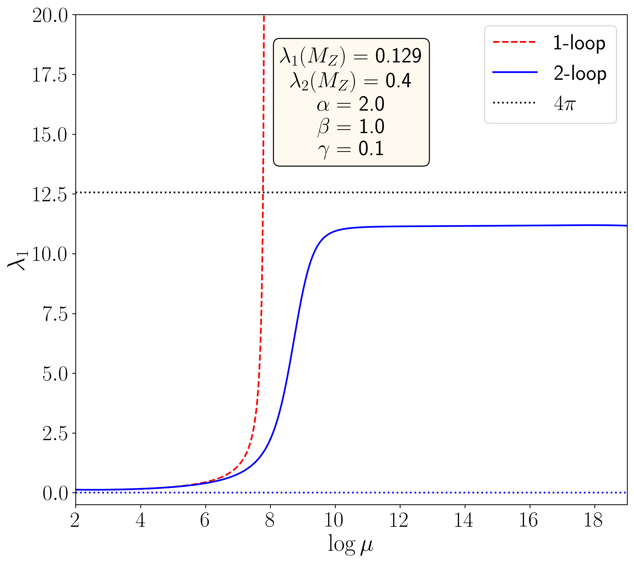
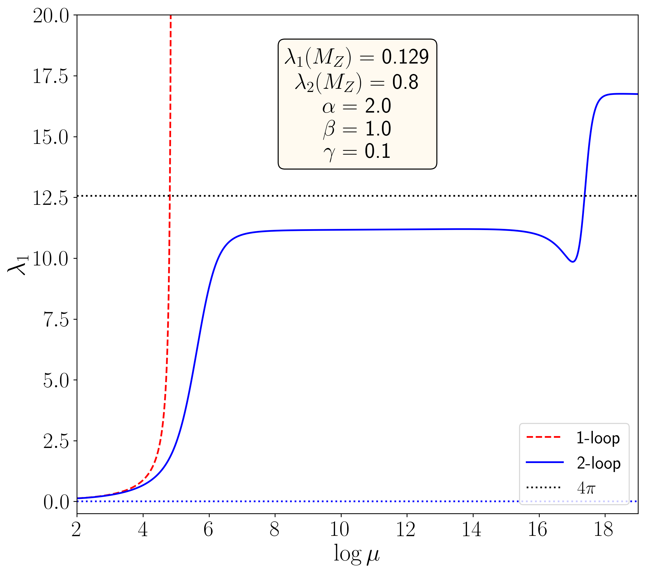
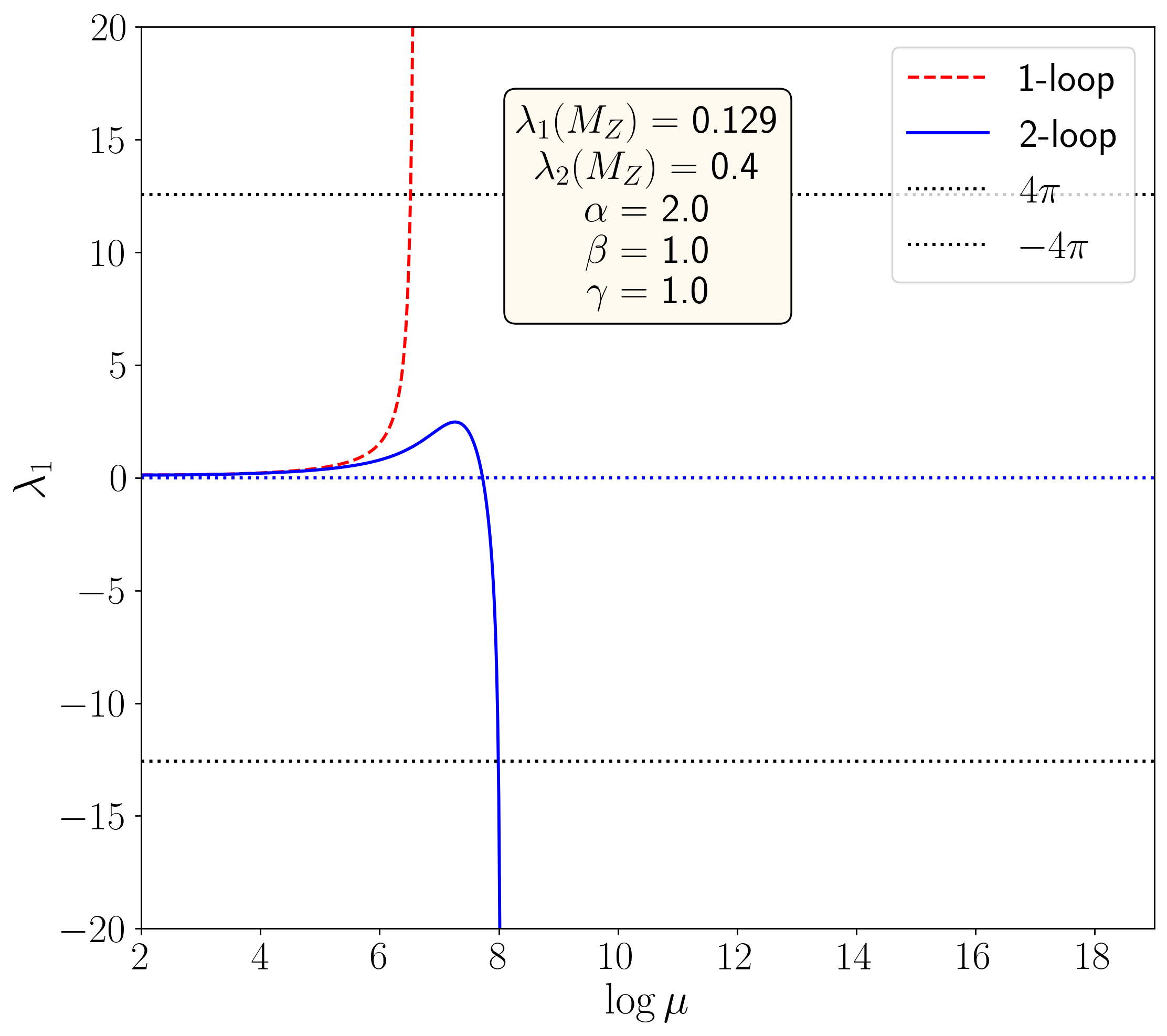
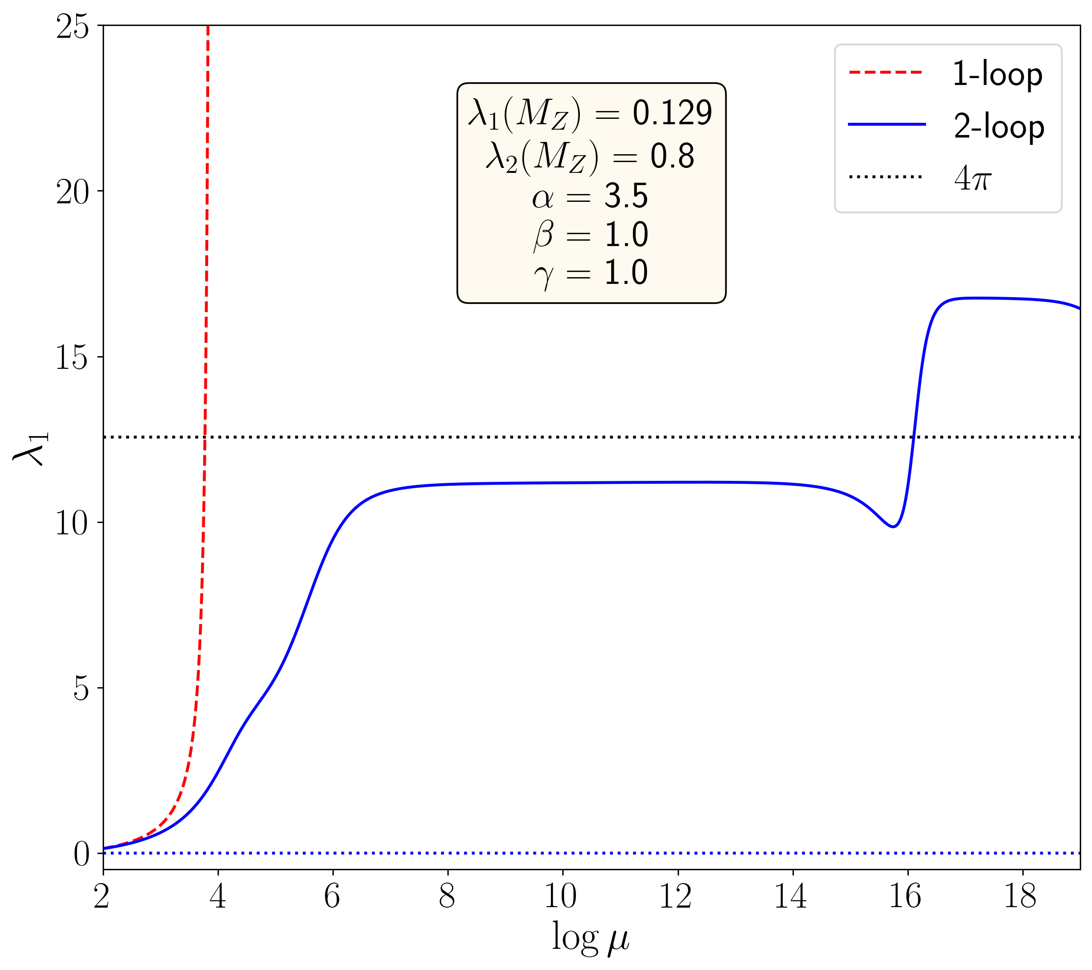
Figure 16: Two-loop RGE evolution of SM Higgs-like quartic coupling in Inert Doublet Model for different fixed values of $\lambda_{i\neq 1}$. Initial value of $\lambda_{H}=0.129$ for all cases. The initial values of $(\lambda_{2},\alpha,\beta,\gamma)$ for (a), (b), (c), and (d) are $(0.4,2.0,1.0,0.1)$, $(0.8,2.0,1.0,0.1)$, $(0.4,2.0,1.0,1.0)$ and $(0.8,3.5,1.0,1.0)$, respectively

From Figure 16 it is clear that there exist FP behaviours in the 2-loop evolution of $\lambda_{1}$ for certain initial values of $\lambda_{2}$, $\lambda_{3}$, $\lambda_{4}$, and $\lambda_{5}$. Figure 16(a) shows that for the choice of $\lambda_{2}=0.4,\alpha=2.0,\beta=1.0,\gamma=0.1$, we see LP at one-loop at $10^{7}$ GeV and FP at the two-loop level at $10^{10}$ GeV, which is similar to $\phi^{4}$-theory, ISM and ITM. For an enhancement of $\lambda_{2}=0.8$, in Figure 16(b), the LP and FP scales reduce to $10^{4},10^{7}$ GeV, respectively. At two-loop with $10^{18}$ GeV, we observe a jump and further FP behaviour like ITM. In Figure 16(c) as we increase the $\gamma=1.0$, the LP and FP both disappear establishing $\gamma$ as a spoiler, which is the artefact of coupling involving $\lambda_{5}$. i.e., term with residual phase. As we sufficiently increase $\alpha=3.5$ in Figure 16(d), we get back both LP and FP, manifesting the $\alpha$ as an enhancer. This will be analysed in detail in the following paragraphs.

In Figure 17 we show the evolution of $\lambda_{2}$ and $\lambda_{3}$, similar to ISM and ITM, for $\alpha=2.0,\,\beta=1.0$, and $\gamma=0.1$. The Fixed points are observed for both $\lambda_{2}$ and $\lambda_{3}$ at the two-loop level around $10^{10}$ GeV. It is worth mentioning that, even though the FP value of $\lambda_{2}$, which is the self-coupling of the inert scalar, stays within the limit of $4\pi$, the FP value for Higgs portal coupling $\lambda_{3}$, crosses $4\pi$, which is similar to the case of ISM and ITM.

  

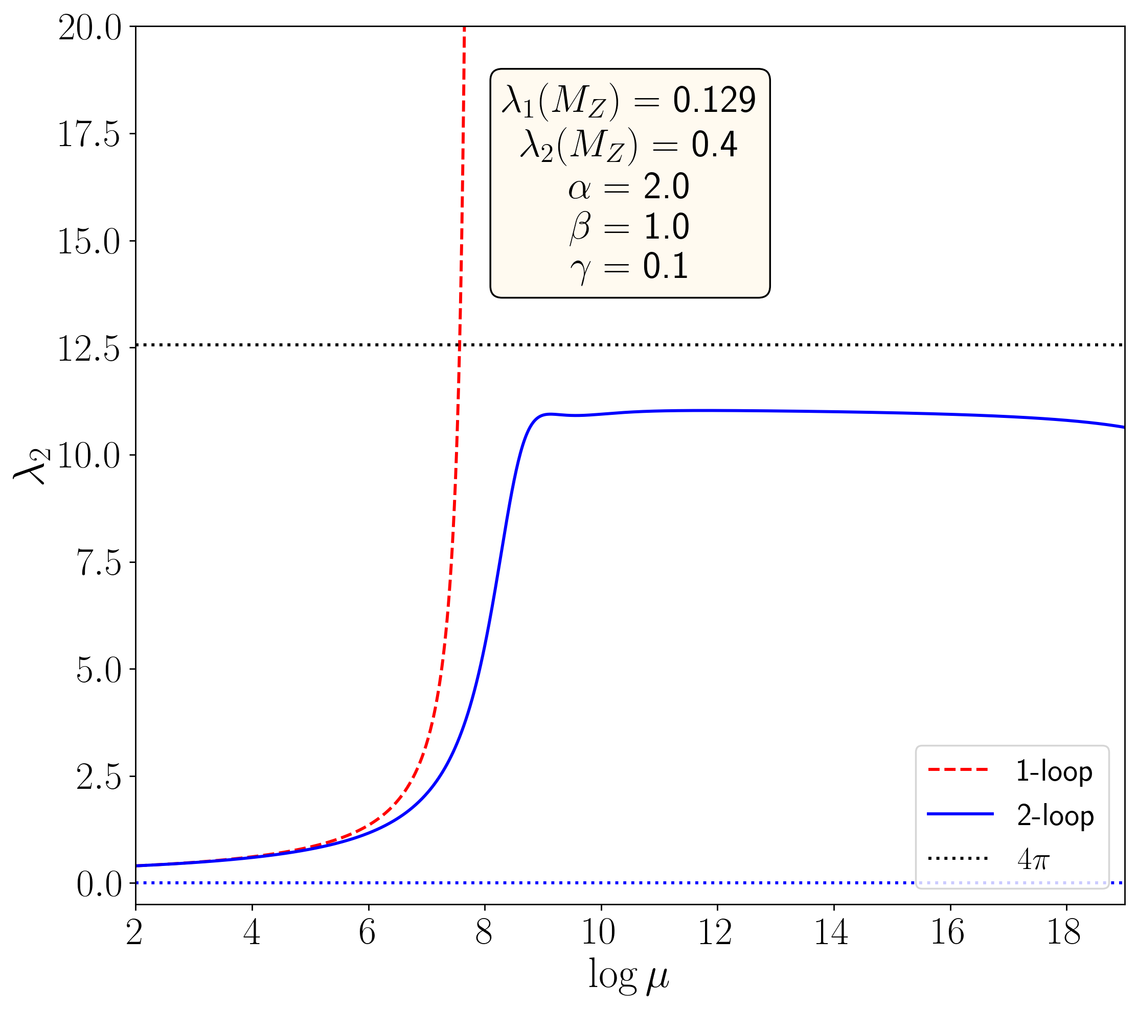
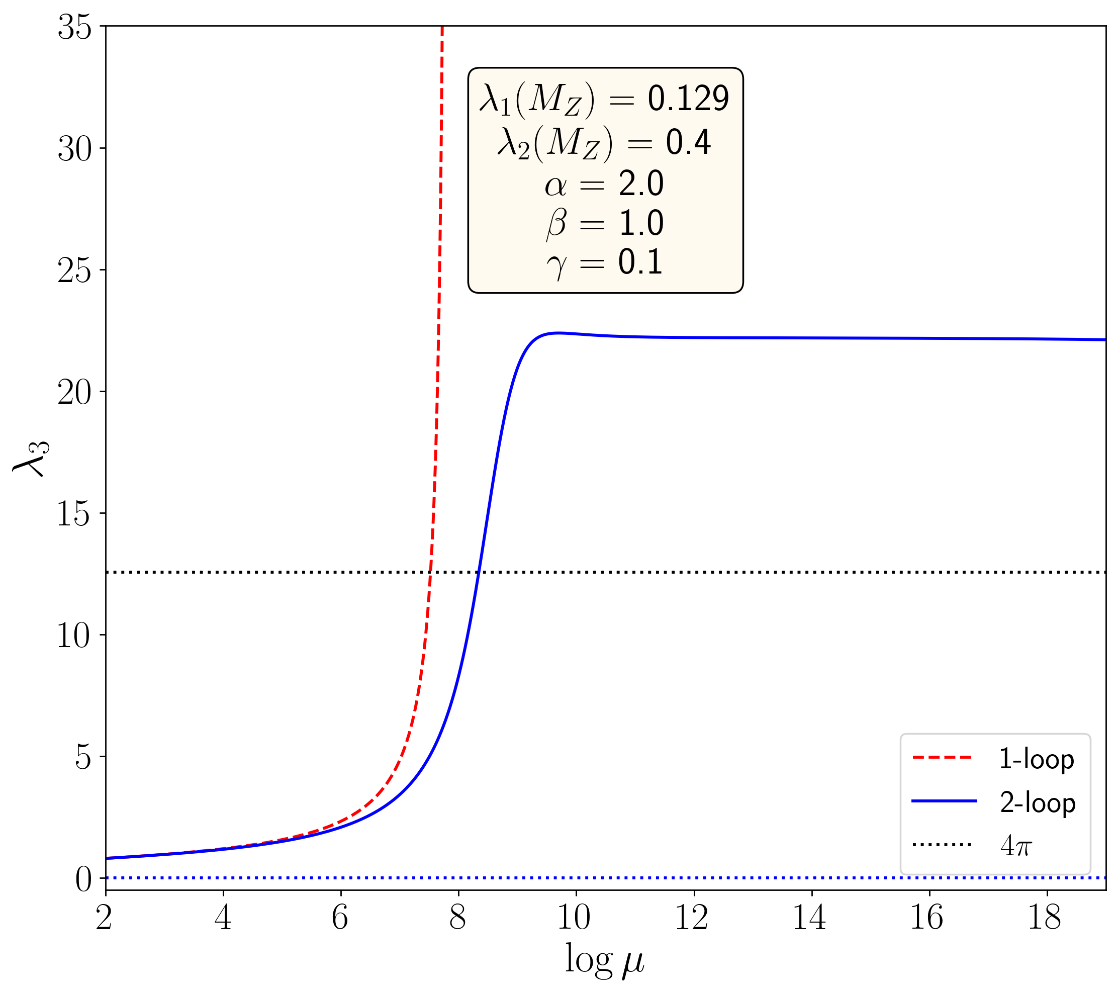
Figure 17: Two-loop RGE evolution of $\lambda_{2}$ and $\lambda_{3}$ in Inert Doublet Model for different fixed values of $\lambda_{i\neq 1}$. Initial value of $\lambda_{H}=0.129$ for all cases. The initial values of $(\lambda_{2},\alpha,\beta,\gamma)$ for (a), and (b) is $(0.4,2.0,1.0,0.1)$, respectively.

To study the role of the relative strengths of $\alpha,\,\beta$ and $\gamma$ we scatter the parameter points in the 2-D plane, where we vary one of the parameters with $\lambda_{2}$, and the scale $t=\log\mu$ is shown in the colour code from blue (7) to yellow (19) while keeping the other two fixed in certain values as we look for the possible Fixed points that start at certain renormalization scale $\mu$ at two-loop.

                 

Figure 18: Occurrence of FP at two-loop in $\lambda_{2}(M_{Z})-\alpha$ plane for different values of $\beta$ and $\gamma$. Initial value of Higgs-self quartic coupling $\lambda_{1}(M_{Z})=0.129$ for all cases.

In Figure 18, we present the variation of $\alpha$ vs $\mu$, where we parametrized some fixed values of $\beta,\gamma$. In Figure 18(a), Figure 18(b), and Figure 18(c), we vary $\alpha$ with respect to $\lambda_{2}(M_{Z})$ while taking $\gamma=0.1,0.5$, and $1.0$, respectively for $\beta=0.5$. There are two things that one can notice here; firstly, greater values of $\lambda_{2}(M_{Z})$ correspond to the appearance of FP at lower scale $t=\log\mu$, and secondly, as we increase the value of $\gamma$ from (a) to (c), the number of points in the parameter space having Fixed points, decreases. Thus $\gamma$ acts as a spoiler for such an FP. As we look for relatively higher values of $\beta=1.0$ in Figure 18(d), (e), (f), the occurrence of FPs reduces further as compared to Figure 18(a), (b), (c), especially for the lower $\alpha$ values. Thus $\beta$ acts like a moderate spoiler. Further increment of $\beta$ to $\beta=1.5$, lessen the occurrence of FPs and for $\beta=1.5,\gamma=1.0$ in Figure 18(i) has no available FPs. For higher values of $\beta,\gamma$ similar observations are found.

                 

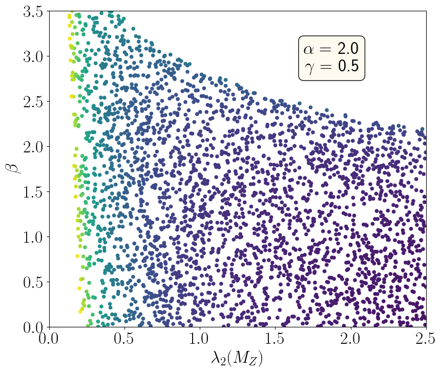
Figure 19: Occurrence of FP at two-loop in $\lambda_{2}(M_{Z})-\beta$ plane for different values of $\alpha$ and $\gamma$. Initial value of Higgs-self quartic coupling $\lambda_{1}(M_{Z})=0.129$ for all cases.

In Figure 19 we vary $\beta$ verse $\lambda_{2}(M_{Z})$ for different values of $\alpha,\gamma$. In Figure 19(a), (b), (c), where we enhance $\gamma$ from $0.1$ to $1.0$, keeping $\alpha=0.1$, two-loop FP occurrences reduce successively from Figure 19(a) to Figure 19(c) as $\gamma$ spoils heavily. For a given $\gamma$ value, an increase in $\alpha$ increases the FP occurrences for relatively smaller values of $\gamma$, which can be seen from Figure 19(d), (e). However, for a larger value of $\gamma=1.0$, the increase of $\alpha=0.5$ is not sufficient, and Figure 19(c) does not have any FP. Nevertheless, if we increase $\alpha$ to an adequate value of $2.0$, FP reappears for all the three values of $\gamma$ as shown in Figure 19(g), (h), (i).

                 

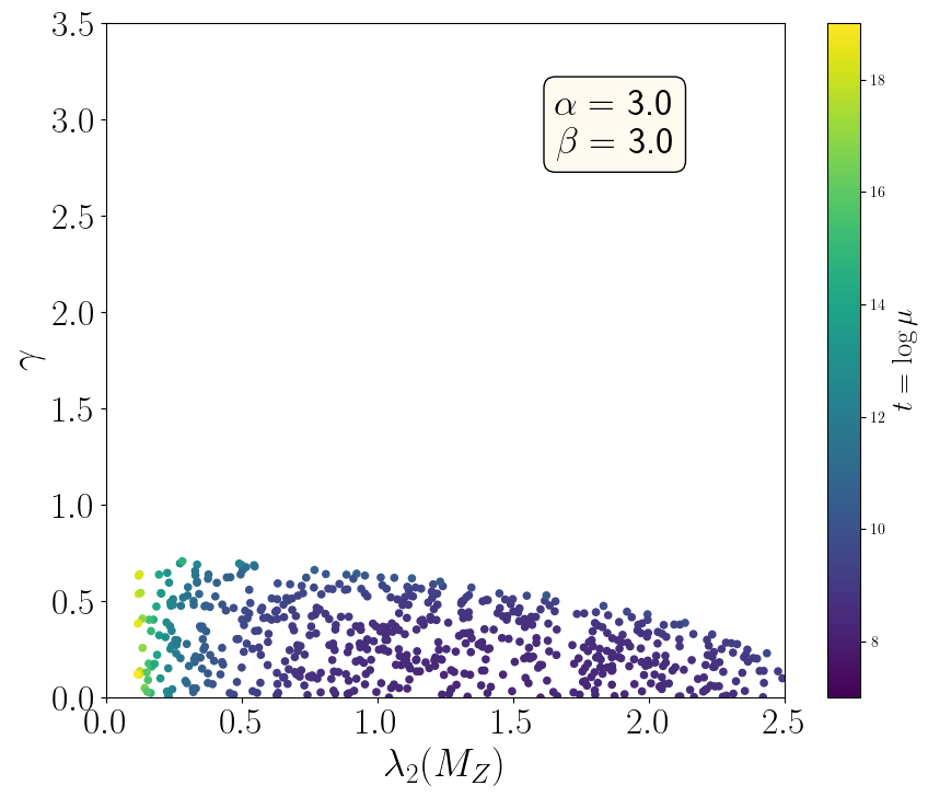
Figure 20: Occurrence of FP at two-loop in $\lambda_{2}(M_{Z})-\gamma$ plane for different values of $\alpha$ and $\beta$. Initial value of Higgs-self quartic coupling $\lambda_{1}(M_{Z})=0.129$ for all cases.

Finally, in Figure 20, we check the occurrence of two-loop FPs in the $\lambda_{2}(M_{Z})-\gamma$ plane for different values of $\alpha$ and $\beta$. In Figure 20(a), (b), (c), we show the Fixed points for $\beta=0.1,\,1.5,\,3.0$ for lower $\alpha=0.1$. It is evident that the available FPs are getting lesser in numbers as we increase $\beta$ values. As we increase the $\alpha$ values column-wise in Figure 20(d), (e), (f) and Figure 20(g), (h), (i) for $\alpha=1.5,\,3.0$, the available FPs increase. This again establishes the behaviour of $\alpha$ as an enhancer and $\beta$ as a moderate spoiler. $\gamma$ being the heavy spoiler, we do not see any fixed point for $\gamma\mathrel{\mathop{\kern 0.0pt\hbox to0.0pt{\raise 0.86108pt\hbox{$>$}\hss}}\lower 3.87495pt\hbox{\kern-1.90002pt$\sim$}}1$.

4.4 IDM Perturbativity Limits

In this subsection we put the perturbativity limits of $4\pi$ in $\lambda_{2}(M_{Z})-\lambda_{3}(M_{Z})$ plane for different scales with different combinations of $\lambda_{4},\,\lambda_{5}$ for both one- and two-loop for IDM using the condition given in Equation 11. Here $\lambda_{2}$ is the new physics self-coupling and $\lambda_{3}$ is the Higgs portal coupling just like in the cases of ISM and ITM. Additionally, we have mixing terms of $\lambda_{4},\lambda_{5}$ and for the first case as described in Figure 21 we consider these terms very small; $\lambda_{4}=\lambda_{5}=0.1$ ensuring minimal interference. The colour code for the perturbativity scale is the same as before. We notice that $\lambda_{2}\lesssim 0.25$ and $\lambda_{3}\lesssim 0.3$ ensures Planck scale perturbativity. For larger couplings at one-loop levels, $\lambda_{2}\gtrsim 1.4,\lambda_{3}\gtrsim 1.5$ the perturbativity scale boils down to $10^{2-3}$ GeV. For higher values of $\lambda_{3}$, the perturbative limits curve down to $10^{2-3}$ for even smaller values of $\lambda_{2}$. Contrary to the previous two cases of ISM and ITM, in the case of IDM, the two-loop perturbativity limits change their shapes for higher values of the couplings. For two-loop, higher values of $\lambda_{2},\lambda_{3}$ are allowed at relatively larger perturbativity scales as in the case of ISM and ITM.

  

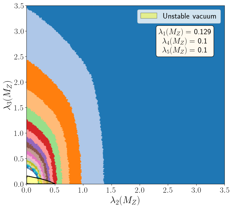
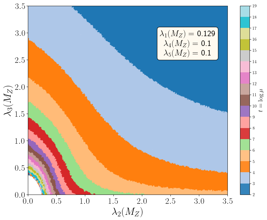
Figure 21: Perturbativity limit of one-loop and two-loop RGE evolution in Inert Doublet Model. Initial value of Higgs-self quartic coupling $\lambda_{H}(M_{Z})=0.129$ and initial values of $\lambda_{4}(M_{Z})=\lambda_{5}(M_{Z})=0.1$ for both cases

We can see in Figure 21(a) the black-contoured yellow-shaded region which corresponds to the parameter region that fails to satisfy the bounded-from-below constraints that are necessary for a stable vacuum, shown in Equation 26. The region has a maximum possible value of $\lambda_{2}(M_{Z})\approx 0.5$ and a maximum possible value of $\lambda_{3}(M_{Z})\approx 0.2$. However, the vacuum becomes stable for the entire parameter region in Figure 21(b) at the two-loop level.

  

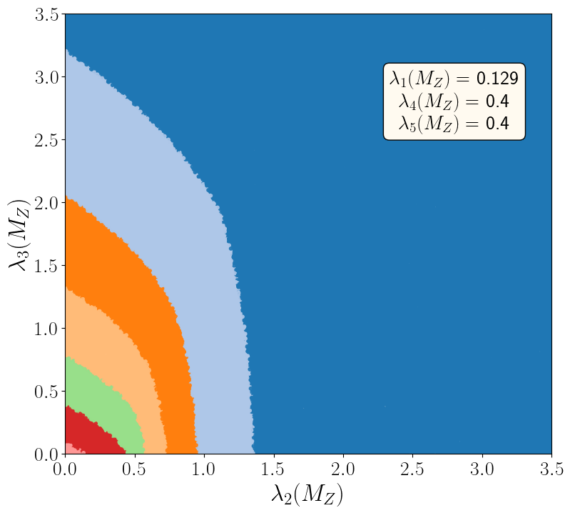
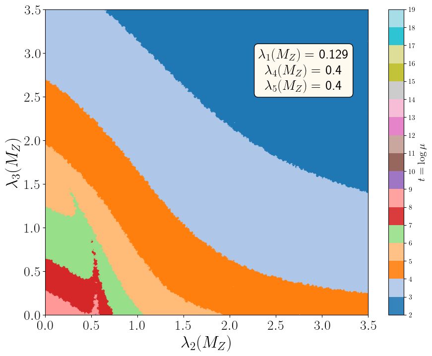
Figure 22: Perturbativity limit of one-loop and two-loop RGE evolution in Inert Doublet Model. Initial value of Higgs-self quartic coupling $\lambda_{H}(M_{Z})=0.129$ and initial values of $\lambda_{4}(M_{Z})=\lambda_{5}(M_{Z})=0.4$ for both cases

Figure 22 describes the situation where the interfering couplings are relatively larger, i.e., $\lambda_{4}=\lambda_{5}=0.4$. The interesting thing to observe is that there is no Planck scale perturbativity possible both at one- and two-loop levels. The maximum perturbative scale that can be achieved is $10^{8-9}$ GeV for lower values of the couplings and the minimum scale that is possible for higher coupling values is $10^{2-3}$ GeV. The two-loop limits are a little relaxed, like before, allowing larger values of the couplings. We also observe a kink-like nature near $\lambda_{2}\sim 0.6$ at the two-loop level owing to the change of sign in the $\beta$-function. For both cases of one- and two-loop, the vacuum stability conditions Equation 26 are satisfied for all the parameter regions in Figure 22.

  

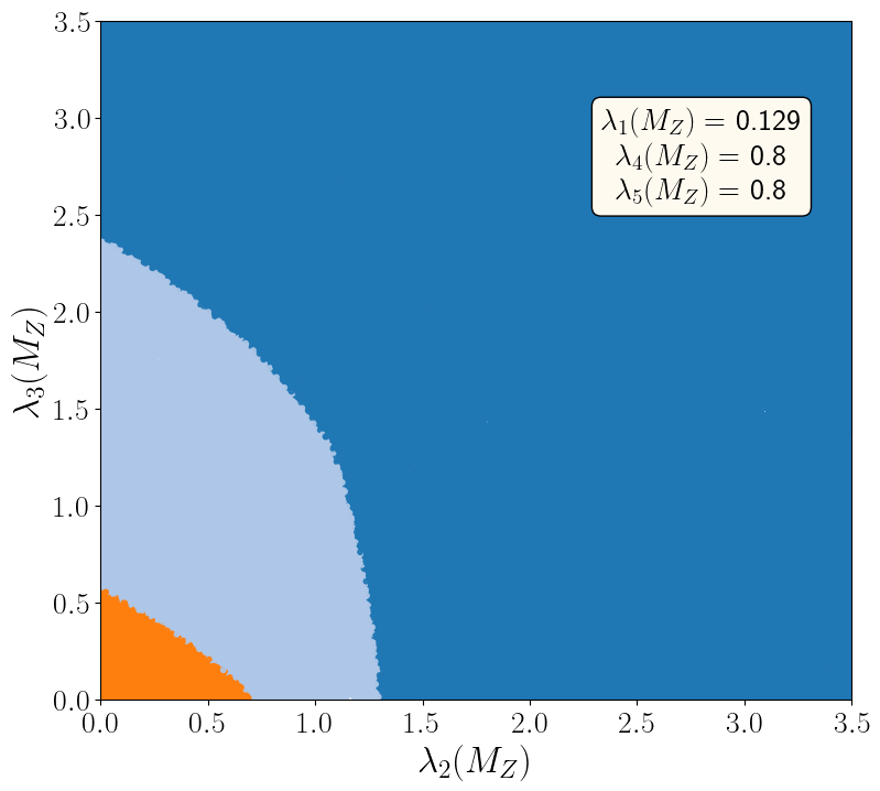
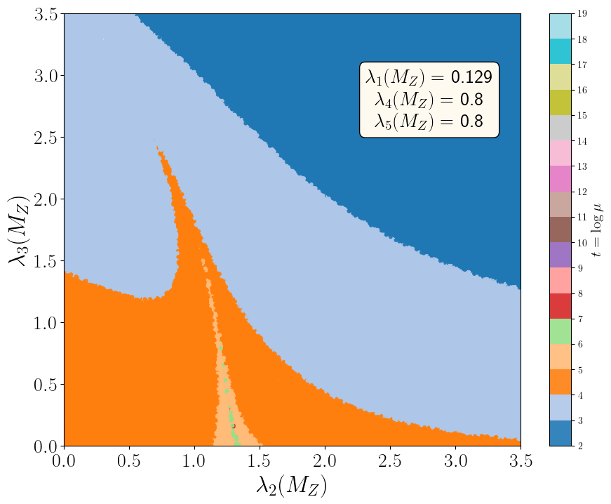
Figure 23: Perturbativity limit of one-loop and two-loop RGE evolution in Inert Doublet Model. Initial value of Higgs-self quartic coupling $\lambda_{H}(M_{Z})=0.129$ and initial values of $\lambda_{4}(M_{Z})=\lambda_{5}(M_{Z})=0.8$ for both cases

In Figure 23 we enhance $\lambda_{4},\lambda_{5}$ to $0.8$. The maximum perturbativity limit comes down to $10^{4-5}$ GeV for lower couplings, while keeping the minimum limit to $10^{2-3}$ GeV for higher values of the couplings. Two-loop limits are more relaxed than one-loop, while the shapes are similar to the previous cases of $\lambda_{4}=\lambda_{5}=0.4$. The kink regions, of course, expose the higher perturbativity limit, i.e. $10^{5-7}$ GeV. Similar to the previous case, for both one- and two-loop, the vacuum stability conditions Equation 26 are satisfied by all points in the parameter space.

  

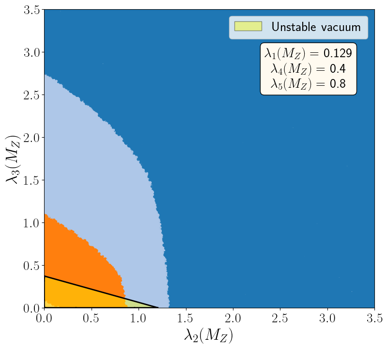
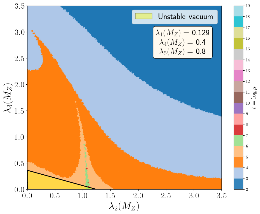
Figure 24: Perturbativity limit of one-loop and two-loop RGE evolution in Inert Doublet Model. Initial value of Higgs-self quartic coupling $\lambda_{H}(M_{Z})=0.129$, initial values of $\lambda_{4}(M_{Z})=0.4$ and initial value of $\lambda_{5}(M_{Z})=0.8$ in both cases.

  

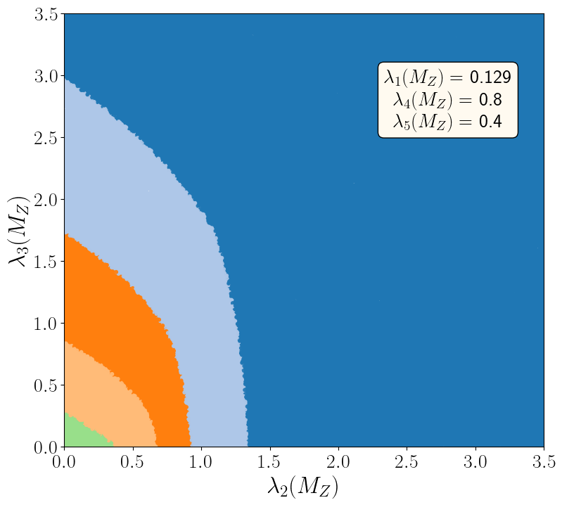
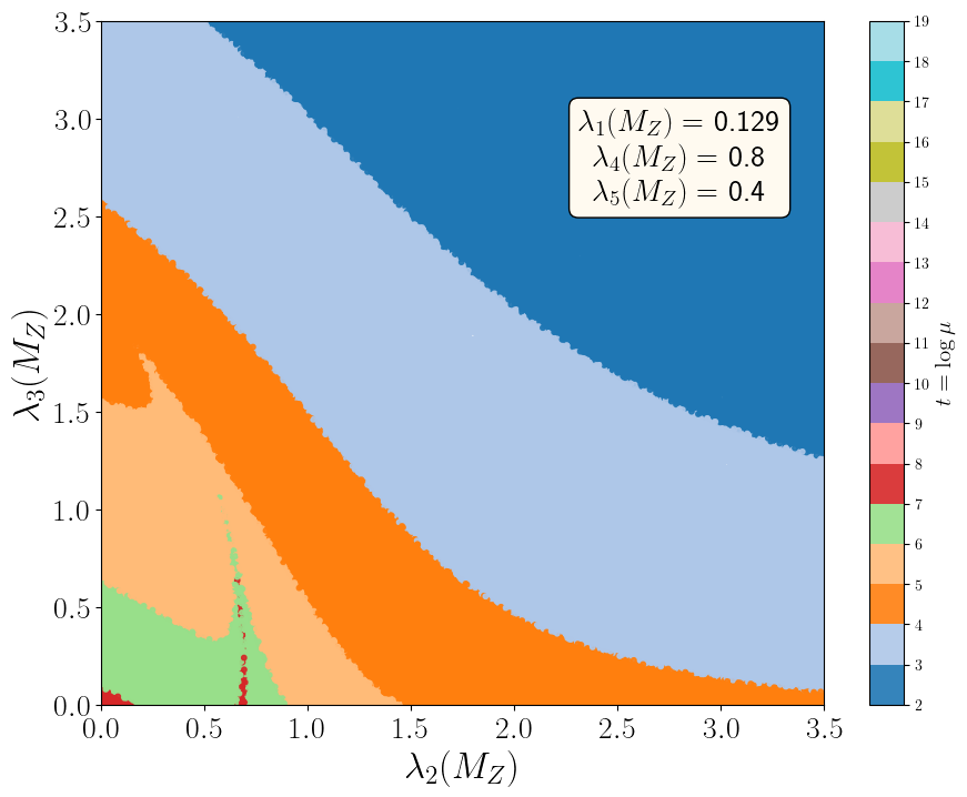
Figure 25: Perturbativity limit of one-loop and two-loop RGE evolution in Inert Doublet Model. Initial value of Higgs-self quartic coupling $\lambda_{H}(M_{Z})=0.129$, initial values of $\lambda_{4}(M_{Z})=0.8$ and initial value of $\lambda_{5}(M_{Z})=0.4$ in both cases.

Figure 24 describes the case for $\lambda_{4}=0.4,\,\lambda_{5}=0.8$. In comparison to the previous case, as depicted in Figure 23, lower couplings are now allowed for a higher perturbativity scale while the higher values of the coupling regions behave similarly. For an opposite choice i.e., $\lambda_{4}=0.8,\,\lambda_{5}=0.4$ as shown in Figure 25, now lower values of $\lambda_{2}$ are allowed for relatively higher perturbativity scales. Similarly, the two-loop kink also shifts toward the left side in the $\lambda_{2}$ axis.

For $\lambda_{4}=0.4,\,\lambda_{5}=0.8$, in Figure 24(a), (b), we can see that there are points within the limits $\lambda_{2}\leq 1.2$ and $\lambda_{3}\leq 0.4$, for which the vacuum is unstable, as shown in the black-contoured yellow-shaded region. However, for the opposite choice $\lambda_{4}=0.8,\,\lambda_{5}=0.4$, in both the one- and two-loop plots, the vacuum is stable for all points as shown in Figure 25.

5 Discussions and Conclusion

In this article, we investigate the RG evolution of the scalar quartic couplings for the inert models, namely inert singlet, inert doublet, and inert triplet models. An interesting feature of having a Landau pole at one-loop and a Fixed point at two-loops for ISM and ITM, which is very similar to the $\phi^{4}$ theory, is noticed. In the $\phi^{4}$-theory, the existence of Landau poles for odd-loops and Fixed points for even loops and their reliability are studied till seven-loop beta-functions six-loop_study_schrock-2016 ; seven-loop_study_schrock-2023 . However, for the Standard Model, no such observation is found till the two-loop level as the initial values of parameters are fixed by the experimental data.

Extending the SM with other scalars: namely ISM, ITM, and IDM, we could invoke more parameters and see the possibility of FPs at the two-loop level in the scalar sector, especially for the the Higgs quartic coupling. We saw that the evolution of SM-like Higgs quartic coupling attains a two-loop FP for certain initial values of parameters. It is mainly governed by the relative strength of portal coupling with the strength of self-coupling of the inert scalar. We observe that in the case of inert singlet and triplet, for small initial values of self-coupling ($\lambda_{S}$ or $\lambda_{T}$), the occurrence of such FPs is promoted by the increase in initial values of the portal couplings ($\lambda_{HS}$ or $\lambda_{HT}$). For higher initial values of $\lambda_{S}$ or $\lambda_{T}$, there is a limit at which portal couplings can promote FPs. Unlike these two cases, the inert doublet has three different portal couplings ($\lambda_{3}$, $\lambda_{4}$, and $\lambda_{5}$) and the latter two behave differently than $\lambda_{3}$. The portal coupling ($\lambda_{3}$) that resembles the singlet/ triplet case, the coefficient of the term that only depends on the square of absolute values of the component fields, promotes the occurrence of such FPs, whereas portal couplings $\lambda_{4}$ and $\lambda_{5}$, which correspond to the terms that have residual phases, suppress the occurrence of FPs. Thus, the appearance of FPs in IDM is not so obvious as $\lambda_{4}$ and $\lambda_{5}$ act as spoilers. Nevertheless, a sufficiently larger value of $\lambda_{3}$ relative to $\lambda_{4,5}$ can bring back the FPs. The residual existing phases from the $\lambda_{4},\lambda_{5}$ terms are instrumental in spoiling the FPs at the two-loop level seven-loop_study_schrock-2023 . In this analysis, we inherited a basis of $\alpha,\,\beta,\,\gamma$, which are the relative strength of $\lambda_{3},\,\lambda_{4},\,\lambda_{5}$ with respect to $\lambda_{2}$, respectively. We found that while the $\alpha$ behaves like an enhancer of the FPs, $\beta$ and $\gamma$ behave like moderate and heavy spoilers of the FP. This will erudite us about the particle behaviour involving the scalar quartic couplings, which will lead to a better understanding of FPs in quantum field theories and help in realizing how they manifest in low-energy interactions.

Considering the conditions for stable vacuum, we see that most of the regions with lower new physics couplings, i.e., $\lambda_{i\neq 1}\lesssim 1.0$ are ruled out, at least for ISM and ITM. However, the situation gets interesting for IDM, as for $\lambda_{4}=\lambda_{5}\mathrel{\mathop{\kern 0.0pt\hbox to0.0pt{\raise 0.86108pt\hbox{$>$}\hss}}\lower 3.87495pt\hbox{\kern-1.90002pt$\sim$}}0.4$, other couplings, i.e., $\lambda_{i=2,3}$ are also allowed even for smaller values, i.e., $\lesssim 1$. A combination of lower $\lambda_{4}$ and greater $\lambda_{5}$, viz., $\lambda_{4}=0.4,\,\lambda_{5}=0.8$, the lower values of other couplings correspond to the unstable vacuum. Thus, perturbative limits are more relevant for higher self and portal couplings.

It is also observed that higher quartic couplings are bounded by relatively lower perturbativity scales, restricting the theory to lower scales. Higher portal couplings are often favoured for FOPT Biekotter:2023eil and even for getting the correct or under-abundant dark matter relics Jangid:2020qgo . In particular, a TeV scale dark matter prefers larger portal couplings Jangid:2020qgo ; Bandyopadhyay:2024plc ; Bandyopadhyay:2023joz . For the scalars in the higher representations of $SU(2)$, to satisfy the current measurement of Higgs to di-photon rate prefers relatively larger portal couplings that are still allowed Bandyopadhyay:2024plc ; Bandyopadhyay:2023joz . If we consider this perturbative unitarity bound on the quartic couplings $\mathrel{\mathop{\kern 0.0pt\hbox to0.0pt{\raise 0.86108pt\hbox{$>$}\hss}}\lower 3.87495pt\hbox{\kern-1.90002pt$\sim$}}1$ , the theory gets non-perturbative at the scale $10^{2-3}$ GeV. In those cases, a multi-TeV dark matter with corresponding large quartic couplings, which are also required to get FOPT, would be questionable while considering perturbativity. Current collider bounds on the scalar quartic couplings are very weak from the di-Higgs productionCMS:2024uru ; CMS:2015jal ; CMS:2024awa ; ATLAS:2023vdy ; ATLAS:2024auw ; ATLAS:2024lsk ; ATLAS:2024xcs , which makes these theoretical estimations more relevant.

Appendix A $\beta$-Functions of the SM and the Inert Models at Two-Loop Level

A.1 Standard Model

$$\beta^{\text{SM}}_{g_{1}} =\frac{1}{(4\pi)^{2}}\left(\frac{41}{10}g_{1}^{3}\right)+\frac{1}{(4\pi)^{4}}\left(\frac{199}{200}g_{1}^{5}+\frac{27}{40}g_{1}^{3}g_{2}^{2}+\frac{11}{5}g_{1}^{3}g_{3}^{2}-\frac{17}{40}g_{1}^{3}Y_{t}^{2}\right)$$ (34)

$$\beta^{\text{SM}}_{g_{2}} =\frac{1}{(4\pi)^{4}}\left(\frac{9}{40}g_{1}^{2}g_{2}^{3}+\frac{35}{24}g_{2}^{5}+3g_{2}^{3}g_{3}^{2}-\frac{3}{8}g_{2}^{3}Y_{t}^{2}\right)+\frac{1}{(4\pi)^{2}}\left(\frac{19}{6}g_{2}^{3}\right)$$ (35)

$$\beta^{\text{SM}}_{g_{3}} =\frac{1}{(4\pi)^{4}}\left(\frac{11}{40}g_{1}^{2}g_{3}^{3}+\frac{9}{8}g_{2}^{2}g_{3}^{3}-\frac{13}{2}g_{3}^{5}-\frac{1}{2}g_{3}^{3}Y_{t}^{2}\right)+\frac{1}{(4\pi)^{2}}\left(7g_{3}^{3}\right)$$ (36)

$$\begin{split}\beta^{\text{SM}}_{Y_{t}}&=\frac{1}{(4\pi)^{2}}\Bigg{(}\frac{9}{32}Y_{t}^{3}+\frac{17}{320}g_{1}^{2}Y_{t}-\frac{9}{64}g_{2}^{2}Y_{t}-\frac{1}{2}g_{3}^{2}Y_{t}\Bigg{)}+\frac{1}{(4\pi)^{4}}\Bigg{(}\frac{1187}{153600}g_{1}^{4}Y_{t}+\\ &+\frac{19}{3840}g_{1}^{2}g_{3}^{2}Y_{t}+\frac{9}{256}g_{2}^{2}g_{3}^{2}Y_{t}+\frac{3}{128}\lambda^{2}Y_{t}+\frac{3}{64}Y_{t}^{5}++\frac{3}{64}\lambda Y_{t}^{3}-\frac{9}{5120}g_{1}^{2}g_{2}^{2}Y_{t}\\ &-\frac{23}{1024}g_{2}^{4}Y_{t}-\frac{27}{64}g_{3}^{4}Y_{t}-\frac{393}{20480}g_{1}^{2}Y_{t}^{3}-\frac{225}{4096}g_{2}^{2}Y_{t}^{3}-\frac{9}{64}g_{3}^{2}Y_{t}^{3}-\frac{9}{32}Y_{t}^{3}\Bigg{)}\end{split}$$ (37)

$$\begin{split}\beta^{\text{SM}}_{\lambda}&=\frac{1}{(4\pi)^{2}}\Bigg{(}\frac{27}{800}g_{1}^{4}+\frac{9}{80}g_{1}^{2}g_{2}^{2}+\frac{9}{32}g_{2}^{4}-\frac{9}{20}g_{1}^{2}\lambda+6\lambda^{2}+3\lambda Y_{t}^{2}-\frac{9}{4}g_{2}^{2}\lambda-\frac{3}{2}Y_{t}^{4}\Bigg{)}\\ &+\frac{1}{(4\pi)^{4}}\Bigg{(}\frac{305}{16}g_{2}^{6}+\frac{1887}{200}g_{1}^{4}\lambda+\frac{117}{20}g_{1}^{2}g_{2}^{2}\lambda+\frac{108}{5}g_{1}^{2}\lambda^{2}+108g_{2}^{2}\lambda^{2}+\frac{63}{10}g_{1}^{2}g_{2}^{2}Y_{t}^{2}+30Y_{t}^{6}\\ &+\frac{17}{2}g_{1}^{2}\lambda Y_{t}^{2}+\frac{45}{2}g_{2}^{2}\lambda Y_{t}^{2}+80g_{3}^{2}\lambda Y_{t}^{2}-\frac{3411}{2000}g_{1}^{6}-\frac{1677}{400}g_{1}^{4}g_{2}^{2}-\frac{289}{80}g_{1}^{2}g_{2}^{4}-\frac{73}{8}g_{2}^{4}\lambda\\ &-312\lambda^{3}-\frac{171}{100}g_{1}^{4}Y_{t}^{2}-\frac{9}{4}g_{2}^{4}Y_{t}^{2}-144\lambda^{2}Y_{t}^{2}-\frac{8}{5}g_{1}^{2}Y_{t}^{4}-32g_{3}^{2}Y_{t}^{4}-3\lambda Y_{t}^{4}\Bigg{)}\end{split}$$

A.2 Inert Singlet Model

$$\beta^{\text{IS}}_{g_{1}} =\beta^{\text{SM}}_{g_{1}},\ \ \ \ \ \ \ \ \ \ \beta^{\text{IS}}_{g_{2}}=\beta^{\text{SM}}_{g_{2}},\ \ \ \ \ \ \ \ \ \ \beta^{\text{IS}}_{g_{3}}=\beta^{\text{SM}}_{g_{3}},\ \ \ \ \ \ \ \ \ \beta^{\text{IS}}_{Y_{t}}=\beta^{\text{SM}}_{Y_{t}}+\frac{1}{2}\lambda_{HS}^{2}Y_{t},$$ (38)

$$\beta^{\text{IS}}_{\lambda_{H}} =\beta^{\text{SM}}_{\lambda_{H}}+\frac{1}{(4\pi)^{2}}\Big{(}\frac{1}{16}\lambda_{HS}^{2}\Big{)}-\frac{1}{(4\pi)^{4}}\Big{(}\frac{5}{128}\lambda_{H}\lambda_{HS}^{2}+\frac{1}{64}\lambda_{HS}^{3}\Big{)}.$$ (39)

$$\begin{split}\beta^{\text{IS}}_{\lambda_{HS}}&=\frac{1}{(4\pi)^{2}}\Big{(}12\lambda_{H}\lambda_{HS}+4\lambda_{HS}^{2}+8\lambda_{HS}\lambda_{S}+6\lambda_{HS}Y_{t}^{2}-\frac{9}{10}g_{1}^{2}\lambda_{HS}-\frac{9}{2}g_{2}^{2}\lambda_{HS}\Big{)}\\ &+\frac{1}{(4\pi)^{4}}\Bigg{(}\frac{1671}{400}g_{1}^{4}\lambda_{HS}+\frac{9}{8}g_{1}^{2}g_{2}^{2}\lambda_{HS}+\frac{72}{5}g_{1}^{2}\lambda_{H}\lambda_{HS}+72g_{2}^{2}\lambda_{H}\lambda_{HS}+\frac{3}{5}g_{1}^{2}\lambda_{HS}^{2}\\ &+3g_{2}^{2}\lambda_{HS}^{2}+\frac{17}{4}g_{1}^{2}\lambda_{HS}Y_{t}^{2}+\frac{45}{4}g_{2}^{2}\lambda_{HS}Y_{t}^{2}+40g_{3}^{2}\lambda_{HS}Y_{t}^{2}-72\lambda_{H}\lambda_{HS}Y_{t}^{2}-12\lambda_{HS}^{2}Y_{t}^{2}\\ &-\frac{27}{2}\lambda_{HS}Y_{t}^{4}-\frac{145}{16}g_{2}^{4}\lambda_{HS}-60\lambda_{H}^{2}\lambda_{HS}-72\lambda_{H}\lambda_{HS}^{2}-11\lambda_{HS}^{3}-48\lambda_{HS}^{2}\lambda_{S}-40\lambda_{HS}\lambda_{S}^{2}\Bigg{)}\end{split}$$

$$\begin{split}\beta^{\text{IS}}_{\lambda_{S}}=&\frac{1}{(4\pi)^{2}}\Big{(}2\lambda_{HS}^{2}+20\lambda_{S}^{2}\Big{)}+\frac{1}{(4\pi)^{4}}\Bigg{(}\frac{12}{5}g_{1}^{2}\lambda_{HS}^{2}+12g_{2}^{2}\lambda_{HS}^{2}-8\lambda_{HS}^{3}-20\lambda_{HS}^{2}\lambda_{S}-240\lambda_{S}^{3}-12\lambda_{HS}^{2}Y_{t}^{2}\Bigg{)}\end{split}$$

A.3 Inert Triplet Model

$$\beta^{\text{ITM}}_{g_{1}} =\beta^{\text{SM}}_{g_{1}},\ \ \ \ \ \ \ \ \ \ \ \beta^{\text{ITM}}_{g_{2}}=\beta^{\text{SM}}_{g_{2}}+\frac{1}{(4\pi)^{2}}\Big{(}\frac{1}{3}g_{2}^{3}\Big{)}+\frac{1}{(4\pi)^{4}}\Big{(}\frac{28}{3}g_{2}^{5}\Big{)}$$ (40)

$$\beta^{\text{ITM}}_{g_{3}} =\beta^{\text{SM}}_{g_{3}},\ \ \ \ \ \ \ \ \ \ \ \beta^{\text{ITM}}_{Y_{t}}=\beta^{\text{SM}}_{Y_{t}}+\frac{1}{(4\pi)^{4}}\Big{(}g_{2}^{4}Y_{t}^{2}+\frac{3}{4}\lambda_{HT}^{2}Y_{t}^{2}\Big{)}$$ (41)

$$\begin{split}\beta^{\text{ITM}}_{\lambda_{H}}=\beta^{\text{SM}}_{\lambda_{H}}+\frac{1}{(4\pi)^{2}}&\Big{(}\frac{3}{2}\lambda_{HT}^{2}\Big{)}+\frac{1}{(4\pi)^{4}}\Big{(}\frac{11}{2}g_{2}^{4}\lambda_{H}+\frac{5}{4}g_{2}^{4}\lambda_{HT}+\frac{9}{2}g_{2}^{2}\lambda_{HT}^{2}\\ &-15\lambda_{H}\lambda_{HT}^{2}-2\lambda_{HT}^{3}-\frac{7}{20}g_{1}^{2}g_{2}^{4}-\frac{7}{4}g_{2}^{6}\Big{)}\end{split}$$ (42)

$$\begin{split}\beta^{\text{ITM}}_{\lambda_{HT}}=&\frac{1}{(4\pi)^{4}}\Big{(}12\lambda_{H}\lambda_{HT}+10\lambda_{HT}\lambda_{T}+6\lambda_{HT}Y_{t}^{2}-\frac{9}{10}g_{1}^{2}\lambda_{HT}-\frac{33}{2}g_{2}^{2}\lambda_{HT}\Big{)}\\ &+\frac{1}{(4\pi)^{4}}\Big{(}\frac{1671}{400}g_{1}^{4}\lambda_{HT}+\frac{9}{8}g_{1}^{2}g_{2}^{2}\lambda_{HT}+\frac{72}{5}g_{1}^{2}\lambda_{H}\lambda_{HT}+72g_{2}^{2}\lambda_{H}\lambda_{HT}+\frac{5}{2}g_{2}^{4}\lambda_{T}\\ &+28g_{2}^{2}\lambda_{HT}\lambda_{T}+\frac{17}{4}g_{1}^{2}\lambda_{HT}Y_{t}^{2}+\frac{45}{4}g_{2}^{2}\lambda_{HT}Y_{t}^{2}+40g_{3}^{2}\lambda_{HT}Y_{t}^{2}-\frac{209}{6}g_{2}^{4}\lambda_{HT}\\ &-60\lambda_{H}^{2}\lambda_{HT}-\frac{23}{2}\lambda_{HT}^{3}-4\lambda_{HT}^{2}\lambda_{T}-26\lambda_{HT}\lambda_{T}^{2}-72\lambda_{H}\lambda_{HT}Y_{t}^{2}-\frac{27}{2}\lambda_{HT}Y_{t}^{4}\Big{)}\end{split}$$ (43)

$$\begin{split}\beta^{\text{ITM}}_{\lambda_{T}}=&\frac{1}{(4\pi)^{4}}\Big{(}\frac{3}{8}g_{2}^{4}+2\lambda_{HT}^{2}+18\lambda_{T}^{2}-24g_{2}^{2}\lambda_{T}\Big{)}+\frac{1}{(4\pi)^{4}}\Big{(}\frac{12}{5}g_{1}^{2}\lambda_{HT}^{2}+12g_{2}^{2}\lambda_{HT}^{2}+54g_{2}^{2}\lambda_{T}^{2}\\ &-\frac{55}{24}g_{2}^{6}-\frac{653}{12}g_{2}^{4}\lambda_{T}-12\lambda_{HT}^{2}\lambda_{T}-156\lambda_{T}^{3}-12\lambda_{HT}^{2}Y_{t}^{2}\Big{)}\end{split}$$ (44)

A.4 Inert Doublet Model

$$\beta^{\text{IDM}}_{g_{1}} =\beta^{\text{SM}}_{g_{1}}+\frac{1}{(4\pi)^{2}}\Big{(}\frac{1}{10}g_{1}^{3}\Big{)}+\frac{1}{(4\pi)^{4}}\Big{(}\frac{9}{50}g_{1}^{5}+\frac{9}{10}g_{1}^{3}g_{2}^{2}\Big{)}$$ (45)

$$\beta^{\text{IDM}}_{g_{2}} =\beta^{\text{SM}}_{g_{2}}+\frac{1}{(4\pi)^{2}}\Big{(}\frac{1}{6}g_{2}^{3}\Big{)}+\frac{1}{(4\pi)^{4}}\Big{(}\frac{3}{10}g_{1}^{2}g_{2}^{3}+\frac{13}{6}g_{2}^{5}\Big{)}$$ (46)

$$\beta^{\text{IDM}}_{g_{3}} =\beta^{\text{SM}}_{g_{3}}$$ (47)

$$\beta^{\text{IDM}}_{Y_{t}} =\beta^{\text{SM}}_{Y_{t}}+\frac{1}{(4\pi)^{4}}\Big{(}\frac{2}{15}g_{1}^{4}Y_{t}+\frac{1}{2}g_{2}^{4}Y_{t}+\lambda_{3}^{2}Y_{t}+\lambda_{3}\lambda_{4}Y_{t}+\lambda_{4}^{2}Y_{t}+6\lambda_{5}^{2}Y_{t}\Big{)}$$ (48)

$$\begin{split}\beta^{\text{IDM}}_{\lambda_{1}}&=\beta^{\text{SM}}_{\lambda_{1}}+\frac{1}{(4\pi)^{2}}\Big{(}2\lambda_{3}^{2}+2\lambda_{3}\lambda_{4}+\lambda_{4}^{2}+4\lambda_{5}^{2}\Big{)}+\frac{1}{(4\pi)^{4}}\Bigg{(}\frac{33}{100}g_{1}^{4}\lambda_{1}+\frac{11}{4}g_{2}^{4}\lambda_{1}+\frac{9}{10}g_{1}^{4}\lambda_{3}+\\ &+\frac{15}{2}g_{2}^{4}\lambda_{3}+\frac{12}{5}g_{1}^{2}\lambda_{3}^{2}+12g_{2}^{2}\lambda_{3}^{2}+\frac{9}{20}g_{1}^{4}\lambda_{4}+\frac{3}{2}g_{1}^{2}g_{2}^{2}\lambda_{4}+\frac{15}{4}g_{2}^{4}\lambda_{4}+\frac{12}{5}g_{1}^{2}\lambda_{3}\lambda_{4}+12g_{2}^{2}\lambda_{3}\lambda_{4}\\ &+\frac{6}{5}g_{1}^{2}\lambda_{4}^{2}+3g_{2}^{2}\lambda_{4}^{2}-\frac{12}{5}g_{1}^{2}\lambda_{5}^{2}-\frac{63}{1000}g_{1}^{6}-\frac{21}{200}g_{1}^{4}g_{2}^{2}-\frac{7}{40}g_{1}^{2}g_{2}^{4}-\frac{7}{8}g_{2}^{6}-20\lambda_{1}\lambda_{3}^{2}-8\lambda_{3}^{3}-20\lambda_{1}\lambda_{3}\lambda_{4}\\ &-12\lambda_{3}^{2}\lambda_{4}-12\lambda_{1}\lambda_{4}^{2}-16\lambda_{3}\lambda_{4}^{2}-6\lambda_{4}^{3}-56\lambda_{1}\lambda_{5}^{2}-80\lambda_{3}\lambda_{5}^{2}-88\lambda_{4}\lambda_{5}^{2}\Bigg{)}\end{split}$$ (49)

$$\begin{split}\beta^{\text{IDM}}_{\lambda_{2}}&=\frac{1}{(4\pi)^{2}}\Big{(}\frac{27}{200}g_{1}^{4}+\frac{9}{20}g_{1}^{2}g_{2}^{2}+\frac{9}{8}g_{2}^{4}+24\lambda_{2}^{2}+2\lambda_{3}^{2}+2\lambda_{3}\lambda_{4}+\lambda_{4}^{2}+4\lambda_{5}^{2}-\frac{9}{5}g_{1}^{2}\lambda_{2}-9g_{2}^{2}\lambda_{2}\Big{)}\\ &+\frac{1}{(4\pi)^{4}}\Bigg{(}\frac{291}{16}g_{2}^{6}+\frac{1953}{200}g_{1}^{4}\lambda_{2}+\frac{117}{20}g_{1}^{2}g_{2}^{2}\lambda_{2}+\frac{108}{5}g_{1}^{2}\lambda_{2}^{2}+108g_{2}^{2}\lambda_{2}^{2}+\frac{9}{10}g_{1}^{4}\lambda_{3}+\frac{15}{2}g_{2}^{4}\lambda_{3}+\frac{12}{5}g_{1}^{2}\lambda_{3}^{2}\\ &+12g_{2}^{2}\lambda_{3}^{2}+\frac{9}{20}g_{1}^{4}\lambda_{4}+\frac{3}{2}g_{1}^{2}g_{2}^{2}\lambda_{4}+\frac{15}{4}g_{2}^{4}\lambda_{4}+\frac{12}{5}g_{1}^{2}\lambda_{3}\lambda_{4}+\frac{6}{5}g_{1}^{2}\lambda_{4}^{2}+3g_{2}^{2}\lambda_{4}^{2}+12g_{2}^{2}\lambda_{3}\lambda_{4}-20\lambda_{2}\lambda_{3}\lambda_{4}\\ &-12\lambda_{3}^{2}\lambda_{4}-\frac{3537}{2000}g_{1}^{6}-\frac{1719}{400}g_{1}^{4}g_{2}^{2}-\frac{303}{80}g_{1}^{2}g_{2}^{4}-\frac{51}{8}g_{2}^{4}\lambda_{2}-312\lambda_{2}^{3}-12\lambda_{2}\lambda_{4}^{2}-16\lambda_{3}\lambda_{4}^{2}-20\lambda_{2}\lambda_{3}^{2}-8\lambda_{3}^{3}\\ &-6\lambda_{4}^{3}-\frac{12}{5}g_{1}^{2}\lambda_{5}^{2}-24\lambda_{5}^{2}Y_{t}^{2}-56\lambda_{2}\lambda_{5}^{2}-80\lambda_{3}\lambda_{5}^{2}-88\lambda_{4}\lambda_{5}^{2}-12\lambda_{3}^{2}Y_{t}^{2}-12\lambda_{3}\lambda_{4}Y_{t}^{2}-6\lambda_{4}^{2}Y_{t}^{2}\Bigg{)}\end{split}$$ (50)

$$\begin{split}\beta^{\text{IDM}}_{\lambda_{3}}&=\frac{1}{(4\pi)^{2}}\Big{(}\frac{27}{100}g_{1}^{4}+\frac{9}{4}g_{2}^{4}+12\lambda_{1}\lambda_{3}+12\lambda_{2}\lambda_{3}+4\lambda_{3}^{2}+4\lambda_{1}\lambda_{4}+4\lambda_{2}\lambda_{4}+2\lambda_{4}^{2}+8\lambda_{5}^{2}\\ &+6\lambda_{3}Y_{t}^{2}-\frac{9}{10}g_{1}^{2}g_{2}^{2}-\frac{9}{5}g_{1}^{2}\lambda_{3}-9g_{2}^{2}\lambda_{3}\Big{)}+\frac{1}{(4\pi)^{2}}\Bigg{(}\frac{909}{200}g_{1}^{4}g_{2}^{2}+\frac{33}{40}g_{1}^{2}g_{2}^{4}\\ &+\frac{291}{8}g_{2}^{6}+\frac{27}{10}g_{1}^{4}\lambda_{1}+\frac{45}{2}g_{2}^{4}\lambda_{1}+\frac{27}{10}g_{1}^{4}\lambda_{2}+\frac{45}{2}g_{2}^{4}\lambda_{2}+\frac{1773}{200}g_{1}^{4}\lambda_{3}+\frac{33}{20}g_{1}^{2}g_{2}^{2}\lambda_{3}\\ &+\frac{72}{5}g_{1}^{2}\lambda_{1}\lambda_{3}+72g_{2}^{2}\lambda_{1}\lambda_{3}+\frac{72}{5}g_{1}^{2}\lambda_{2}\lambda_{3}+72g_{2}^{2}\lambda_{2}\lambda_{3}+\frac{6}{5}g_{1}^{2}\lambda_{3}^{2}+6g_{2}^{2}\lambda_{3}^{2}+\frac{15}{2}g_{2}^{4}\lambda_{4}\\ &+\frac{9}{10}g_{1}^{4}\lambda_{4}+\frac{24}{5}g_{1}^{2}\lambda_{1}\lambda_{4}+6g_{2}^{2}\lambda_{4}^{2}+36g_{2}^{2}\lambda_{1}\lambda_{4}+\frac{48}{5}g_{1}^{2}\lambda_{5}^{2}+\frac{24}{5}g_{1}^{2}\lambda_{2}\lambda_{4}+\frac{17}{4}g_{1}^{2}\lambda_{3}Y_{t}^{2}\\ &+\frac{45}{4}g_{2}^{2}\lambda_{3}Y_{t}^{2}+40g_{3}^{2}\lambda_{3}Y_{t}^{2}+36g_{2}^{2}\lambda_{2}\lambda_{4}-72\lambda_{2}\lambda_{3}^{2}-12\lambda_{3}^{3}-\frac{3537}{1000}g_{1}^{6}-3g_{1}^{2}g_{2}^{2}\lambda_{1}\\ &-3g_{1}^{2}g_{2}^{2}\lambda_{2}-72\lambda_{1}\lambda_{3}^{2}-\frac{111}{8}g_{2}^{4}\lambda_{3}-60\lambda_{1}^{2}\lambda_{3}-60\lambda_{2}^{2}\lambda_{3}-\frac{9}{5}g_{1}^{2}g_{2}^{2}\lambda_{4}-16\lambda_{1}^{2}\lambda_{4}\\ &-16\lambda_{2}^{2}\lambda_{4}-12g_{2}^{2}\lambda_{3}\lambda_{4}-32\lambda_{1}\lambda_{3}\lambda_{4}-32\lambda_{2}\lambda_{3}\lambda_{4}-4\lambda_{3}^{2}\lambda_{4}-\frac{6}{5}g_{1}^{2}\lambda_{4}^{2}-28\lambda_{1}\lambda_{4}^{2}\\ &-28\lambda_{2}\lambda_{4}^{2}-16\lambda_{3}\lambda_{4}^{2}-12\lambda_{4}^{3}-144\lambda_{1}\lambda_{5}^{2}-144\lambda_{2}\lambda_{5}^{2}-72\lambda_{3}\lambda_{5}^{2}-176\lambda_{4}\lambda_{5}^{2}\\ &-\frac{171}{100}g_{1}^{4}Y_{t}^{2}-\frac{63}{10}g_{1}^{2}g_{2}^{2}Y_{t}^{2}-\frac{9}{4}g_{2}^{4}Y_{t}^{2}-72\lambda_{1}\lambda_{3}Y_{t}^{2}-12\lambda_{3}^{2}Y_{t}^{2}-24\lambda_{1}\lambda_{4}Y_{t}^{2}-6\lambda_{4}^{2}Y_{t}^{2}\\ &-24\lambda_{5}^{2}Y_{t}^{2}-\frac{27}{2}\lambda_{3}Y_{t}^{4}\Bigg{)}\end{split}$$ (51)

$$\begin{split}\beta^{\text{IDM}}_{\lambda_{4}}=&\frac{1}{(4\pi)^{2}}\Big{(}\frac{9}{5}g_{1}^{2}g_{2}^{2}+4\lambda_{1}\lambda_{4}+4\lambda_{2}\lambda_{4}+8\lambda_{3}\lambda_{4}+4\lambda_{4}^{2}+32\lambda_{5}^{2}+6\lambda_{4}Y_{t}^{2}-\frac{9}{5}g_{1}^{2}\lambda_{4}-9g_{2}^{2}\lambda_{4}\Big{)}\\ &+\frac{1}{(4\pi)^{2}}\Bigg{(}6g_{1}^{2}g_{2}^{2}\lambda_{1}+6g_{1}^{2}g_{2}^{2}\lambda_{2}+\frac{6}{5}g_{1}^{2}g_{2}^{2}\lambda_{3}+\frac{1413}{200}g_{1}^{4}\lambda_{4}+\frac{153}{20}g_{1}^{2}g_{2}^{2}\lambda_{4}\lambda_{5}^{2}+\frac{63}{5}g_{1}^{2}g_{2}^{2}Y_{t}^{2}\\ &+\frac{17}{4}g_{1}^{2}\lambda_{4}Y_{t}^{2}+\frac{45}{4}g_{2}^{2}\lambda_{4}Y_{t}^{2}+40g_{3}^{2}\lambda_{4}Y_{t}^{2}+\frac{24}{5}g_{1}^{2}\lambda_{1}\lambda_{4}+\frac{24}{5}g_{1}^{2}\lambda_{2}\lambda_{4}\\ &+\frac{12}{5}g_{1}^{2}\lambda_{3}\lambda_{4}+36g_{2}^{2}\lambda_{3}\lambda_{4}+\frac{24}{5}g_{1}^{2}\lambda_{4}^{2}+18g_{2}^{2}\lambda_{4}^{2}+\frac{192}{5}g_{1}^{2}\lambda_{5}^{2}+216g_{2}^{2}\lambda_{5}^{2}-40\lambda_{1}\lambda_{4}^{2}\\ &-40\lambda_{2}\lambda_{4}^{2}-28\lambda_{3}\lambda_{4}^{2}-\frac{657}{50}g_{1}^{4}g_{2}^{2}-\frac{42}{5}g_{1}^{2}g_{2}^{4}-\frac{231}{8}g_{2}^{4}\lambda_{4}-28\lambda_{1}^{2}\lambda_{4}-28\lambda_{2}^{2}\lambda_{4}\\ &-80\lambda_{1}\lambda_{3}\lambda_{4}-80\lambda_{2}\lambda_{3}\lambda_{4}-28\lambda_{3}^{2}\lambda_{4}-192\lambda_{1}\lambda_{5}^{2}-192\lambda_{2}\lambda_{5}^{2}-192\lambda_{3}\lambda_{5}^{2}-104\lambda_{4}\\ &-24\lambda_{1}\lambda_{4}Y_{t}^{2}-24\lambda_{3}\lambda_{4}Y_{t}^{2}-12\lambda_{4}^{2}Y_{t}^{2}-96\lambda_{5}^{2}Y_{t}^{2}-\frac{27}{2}\lambda_{4}Y_{t}^{4}\Bigg{)}\end{split}$$ (52)

$$\begin{split}\beta^{\text{IDM}}_{\lambda_{5}}=&\frac{1}{(4\pi)^{2}}\Big{(}4\lambda_{1}\lambda_{5}+4\lambda_{2}\lambda_{5}+8\lambda_{3}\lambda_{5}+12\lambda_{4}\lambda_{5}+6\lambda_{5}Y_{t}^{2}-\frac{9}{5}g_{1}^{2}\lambda_{5}-9g_{2}^{2}\lambda_{5}\Big{)}\\ &+\frac{1}{(4\pi)^{4}}\Bigg{(}\frac{1413}{200}g_{1}^{4}\lambda_{5}+\frac{57}{20}g_{1}^{2}g_{2}^{2}\lambda_{5}+\frac{48}{5}g_{1}^{2}\lambda_{3}\lambda_{5}+36g_{2}^{2}\lambda_{3}\lambda_{5}+\frac{72}{5}g_{1}^{2}\lambda_{4}\lambda_{5}\\ &+72g_{2}^{2}\lambda_{4}\lambda_{5}+24\lambda_{5}^{3}+\frac{171}{200}g_{1}^{4}Y_{t}^{2}+\frac{9}{8}g_{2}^{4}Y_{t}^{2}+\frac{17}{4}g_{1}^{2}\lambda_{5}Y_{t}^{2}+\frac{45}{4}g_{2}^{2}\lambda_{5}Y_{t}^{2}\\ &+40g_{3}^{2}\lambda_{5}Y_{t}^{2}+\frac{9}{2}\lambda_{5}Y_{t}^{4}-\frac{231}{8}g_{2}^{4}\lambda_{5}-\frac{12}{5}g_{1}^{2}\lambda_{1}\lambda_{5}-28\lambda_{1}^{2}\lambda_{5}-\frac{12}{5}g_{1}^{2}\lambda_{2}\lambda_{5}\\ &-28\lambda_{2}^{2}\lambda_{5}-80\lambda_{1}\lambda_{3}\lambda_{5}-80\lambda_{2}\lambda_{3}\lambda_{5}-28\lambda_{3}^{2}\lambda_{5}-88\lambda_{1}\lambda_{4}\lambda_{5}-88\lambda_{2}\lambda_{4}\lambda_{5}\\ &-76\lambda_{3}\lambda_{4}\lambda_{5}-32\lambda_{4}^{2}\lambda_{5}-\frac{63}{20}g_{1}^{2}g_{2}^{2}Y_{t}^{2}-24\lambda_{1}\lambda_{5}Y_{t}^{2}-24\lambda_{3}\lambda_{5}Y_{t}^{2}-36\lambda_{4}\lambda_{5}Y_{t}^{2}\Bigg{)}\end{split}$$ (53)

References

- (1) G. Aad et al. [ATLAS Collaboration], Observation of a new particle in the search for the Standard Model Higgs boson with the ATLAS detector at the LHC, Phys. Lett. B 716, 1 (2012) [arXiv:1207.7214 [hep-ex]].
- (2) S. Chatrchyan et al. [CMS Collaboration], Observation of a new boson at a mass of 125 GeV with the CMS experiment at the LHC, Phys. Lett. B 716, 30 (2012) [arXiv:1207.7235 [hep-ex]].
- (3) G. Isidori, G. Ridolfi and A. Strumia, On the metastability of the Standard Model vacuum, Nucl. Phys. B 609, 3 (2001), 387-409 [hep-ph/0104016].
- (4) F. Bezrukov, M.Y. Kalmykov, B. A. Kniehl and M. Shaposhnikov, Higgs boson mass and new physics, JHEP 1210, 140 (2012) [arXiv:1205.2893 [hep-ph]].
- (5) G. Degrassi, S. Di Vita, J. Elias-Miro, J. R. Espinosa, G. F. Giudice, G. Isidori and A. Strumia, Higgs mass and vacuum stability in the Standard Model at NNLO, JHEP 1208, 098 (2012) [arXiv:1205.6497 [hep-ph]].
- (6) D. Buttazzo, G. Degrassi, P. P. Giardino, G. F. Giudice, F. Sala, A. Salvio and A. Strumia, Investigating the near-criticality of the Higgs boson, JHEP 1312, 089 (2013) [arXiv:1307.3536 [hep-ph]].
- (7) F. Csikor, Z. Fodor, and J. Heitger, End Point of the Hot Electroweak Phase Transition, Phys. Rev. Lett. 82, 21 (1999).
- (8) K. Rummukainen, M. Tsypin, K. Kajantie, M. Laine, and M. E. Shaposhnikov, The universality class of the electroweak theory, Nucl. Phys. B532, 283 (1998).
- (9) K. Kajantie, M. Laine, K. Rummukainen, and M. E. Shaposhnikov, Is There a Hot Electroweak Phase Transition at ?, Phys. Rev. Lett. 77, 2887 (1996).
- (10) M. Gonderinger, Y. Li, H. Patel and M. J. Ramsey-Musolf, Vacuum stability, perturbativity, and scalar singlet dark matter, JHEP 1001, 053 (2010) [arXiv:0910.3167 [hep-ph]].
- (11) M. Gonderinger, H. Lim and M. J. Ramsey-Musolf, Complex scalar singlet dark matter: Vacuum stability and phenomenology, Phys. Rev. D 86, 043511 (2012) [arXiv:1202.1316 [hep-ph]].
- (12) O. Lebedev, On stability of the electroweak vacuum and the Higgs portal, Eur. Phys. J. C 72, 2058 (2012) [arXiv:1203.0156 [hep-ph]].
- (13) J. Elias-Miro, J. R. Espinosa, G. F. Giudice, H. M. Lee and A. Strumia, Stabilization of the electroweak vacuum by a scalar threshold effect, JHEP 1206, 031 (2012) [arXiv:1203.0237 [hep-ph]].
- (14) P. Athron, J. M. Cornell, F. Kahlhoefer, J. Mckay, P. Scott and S. Wild, Impact of vacuum stability, perturbativity and XENON1T on global fits of and scalar singlet dark matter, Eur. Phys. J. C 78, no. 10, 830 (2018) [arXiv:1806.11281 [hep-ph]].
- (15) V. Barger, P. Langacker, M. McCaskey, M. Ramsey-Musolf, and G. Shaughnessy, Complex singlet extension of the standard model, Phy. Rev. D 79, 015018 (2009).
- (16) G. C. Branco, P. M. Ferreira, L. Lavoura, M. N. Rebelo, M. Sher, and J. P. Silva, Theory and phenomenology of two-Higgs-doublet models Phys. Rep. 516, 1 (2012).
- (17) P. M. Ferreira, R. Santos and A. Barroso, Stability of the tree-level vacuum in two Higgs doublet models against charge or CP spontaneous violation, Phys. Lett. B 603, 219 (2004) Erratum: [Phys. Lett. B 629, 114 (2005)] [hep-ph/0406231].
- (18) M. Maniatis, A. von Manteuffel, O. Nachtmann and F. Nagel, Stability and symmetry breaking in the general two-Higgs-doublet model, Eur. Phys. J. C 48, 805 (2006) [hep-ph/0605184].
- (19) L. L. Honorez, E. Nezri, J. F. Oliver and M. H. G. Tytgat, The inert doublet model: an archetype for dark matter, JCAP 02 (2007) 028
- (20) N. Khan, S. Rakshit, Constraints on inert dark matter from the metastability of the electroweak vacuum, Phys. Rev. D 92, 055006 (2015) [arXiv:1503.03085 [hep-ph]].
- (21) X. J. Xu, Tree-level vacuum stability of two-Higgs-doublet models and new constraints on the scalar potential, Phys. Rev. D 95, no. 11, 115019 (2017) [arXiv:1705.08965 [hep-ph]].
- (22) K. Kannike, Vacuum stability of a general scalar potential of a few fields, Eur. Phys. J. C 76, no. 6, 324 (2016) Erratum: [Eur. Phys. J. C 78, no. 5, 355 (2018)] [arXiv:1603.02680 [hep-ph]].
- (23) S. Jangid and P. Bandyopadhyay, Distinguishing Inert Higgs Doublet and Inert Triplet Scenarios, Eur. Phys. J. C 80 (2020) no.8, 715 doi:10.1140/epjc/s10052-020-8271-5 [arXiv:2003.11821 [hep-ph]].
- (24) P. Bandyopadhyay, M. Frank, S. Parashar and C. Sen, Interplay of inert doublet and vector-like lepton triplet with displaced vertices at the LHC/FCC and MATHUSLA, JHEP 03, 109 (2024) doi:10.1007/JHEP03(2024)109 [arXiv:2310.08883 [hep-ph]].
- (25) Nico Benincasa, Luigi Delle Rose, Kristen Kannike and Luca Marzola, Multi-step Phase Transitions and Gravitational Waves in the Inert Doublet Model, JCAP 12(2022)025 . DOI:https://doi.org/10.1088/1475-7516/2022/12/025
- (26) P. Bandyopadhyay and R. Mandal, Vacuum stability in an extended standard model with a leptoquark, Phys. Rev. D 95, no.3, 035007 (2017) doi:10.1103/PhysRevD.95.035007 [arXiv:1609.03561 [hep-ph]].
- (27) S. Yaser Ayazi and S. M. Firouzabadi, Footprint of triplet scalar dark matter in direct, indirect search and invisible Higgs decay, Cogent Phys. 2 1047559 (2015) [arXiv:1501.06176 [hep-ph]].
- (28) N. Khan, Exploring the hyperchargeless Higgs triplet model up to the Planck scale, Eur. Phys. J. C 78 no.4, 341 (2018) [arXiv:1610.03178 [hep-ph]].
- (29) P. Bandyopadhyay, S. Parashar, C. Sen and J. Song, Probing Inert Triplet Model at a multi-TeV muon collider via vector boson fusion with forward muon tagging, JHEP 07 (2024), 253 doi:10.1007/JHEP07(2024)253 [arXiv:2401.02697 [hep-ph]].
- (30) N. Chakrabarty, D. K. Ghosh, B. Mukhopadhyaya and I. Saha, Dark matter, neutrino masses, and high scale validity of an inert Higgs doublet model, Phys. Rev. D 92 (2015) no.1, 015002 [arXiv:1501.03700 [hep-ph]].
- (31) B. Swiezewska, Inert scalars and vacuum metastability around the electroweak scale, JHEP 07 (2015) 118 [arXiv:1503.07078 [hep-ph]].
- (32) P. Bandyopadhyay, P. S. B. Dev, S. Jangid, and A. Kumar, Vacuum stability in inert higgs doublet model with right-handed neutrinos, JHEP 08 (2020) 154 [arXiv:2001.01764 [hep-ph]].
- (33) P. Bandyopadhyay and S. Jangid, Discerning singlet and triplet scalars at the electroweak phase transition and gravitational wave, Phys. Rev. D 107, (2023) 055032, [arXiv:2111.03866 [hep-ph]].
- (34) P. Bandyopadhyay and S. Jangid, Scrutinizing Vacuum Stability in IDM with Type-III Inverse Seesaw, JHEP 02 (2021) 075, [arXiv:2008.11956 [hep-ph]].
- (35) D. Eriksson, J. Rathsman and O. Stal, 2HDMC: Two-Higgs-Doublet Model Calculator Physics and Manual, Comput. Phys. Commun. 181, 189-205 (2010) doi:10.1016/j.cpc.2009.09.011 [arXiv:0902.0851 [hep-ph]]. [15:02, 21/04/2025] Pram IITH:
- (36) C. Grojean, G. Servant and J. D. Wells, First-order electroweak phase transition in the standard model with a low cutoff, Phy. Rev. D 71 036001 (2005) [hep-ph/0407019 [hep-ph]].
- (37) A. Ahriche, What is the criterion for a strong first-order electroweak phase transition in singlet models?, Phys. Rev. D 75 (2007) 083522, [hep-ph/0701192].
- (38) J. R. Espinosa, T. Konstandin and F. Riva, Strong Electroweak Phase Transitions in the Standard Model with a Singlet, Nucl. Phys. B 854 (2012) 592–630, [arXiv:1107.5441 [hep-ph]].
- (39) M. D. Astros, S. Fabian and F. Goertz, Minimal Inert Doublet benchmark for dark matter and the baryon asymmetry, JCAP02(2024)052, DOI: 10.1088/1475-7516/2024/02/052
- (40) S. AbdusSalam, M. J. Kazemi, and L. Kalhor,, Upper limit on first-order electroweak phase transition strength , International Journal of Modern Physics A Vol. 36, No. 05, 2150024 (2021), DOI: https://doi.org/10.1142/S0217751X2150024X
- (41) D. Borah and J. M. Cline, Inert doublet dark matter with strong electroweak phase transition, Phy. Rev. D 86 055001 (2012).
- (42) G. Gil, P. Chankowski and M. Krawczyk, Inert dark matter and strong electroweak phase transition, Phys. Lett. B 717 (2012) 396–402.
- (43) J. M. Cline and K. Kainulainen, Improved electroweak phase transition with subdominant inert doublet dark matter, Phys. Rev. D 87, 071701(R) (2013).
- (44) S. S. AbdusSalam and T. A. Chowdhury, Scalar representations in the light of electroweak phase transition and cold dark matter phenomenology, JCAP 05 (2014) 026, 026–026 [arXiv:1310.8152 [hep-ph]].
- (45) S. S. AbdusSalam and M. J. Kazemi, Electroweak phase transition in an inert complex triplet mode, Phys. Rev. D 103, 075012 (2021).
- (46) P. Bandyopadhyay, S. Jangid, and A. Karan, Constraining scalar doublet and triplet leptoquarks with vacuum stability and perturbativity, arXiv:2111.03872, doi: 10.1140/epjc/s10052-022-10418-6
- (47) Y. Hamada, K. Kawana and K. Tsumura, Landau pole in the Standard Model with weakly interacting scalar fields, Phys. Lett. B 747, 238-244 (2015) doi:10.1016/j.physletb.2015.05.072 [arXiv:1505.01721 [hep-ph]].
- (48) A. D. Bond, G. Hiller, K. Kowalska and D. F. Litim, Directions for model building from asymptotic safety, JHEP 08, 004 (2017) doi:10.1007/JHEP08(2017)004 [arXiv:1702.01727 [hep-ph]].
- (49) S. Heinemeyer, M. Mondragón, N. Tracas, and G. Zoupanos, Reduction of couplings and its application in particle physics, Phys. Rept., 814 (2019), Pages 1-43.
- (50) M. A. May Pech, M. Mondragón, G. Patellis, and G. Zoupanos, Reduction of couplings in the Type-II 2HDM, Eur. J. Phys. 83 (2023), article number 1129.
- (51) R. Shrock, Study of the six-loop beta function of the theory, Phys. Rev. D, 94 (2016), 125026.
- (52) R. Shrock, Search for an ultraviolet zero in the seven-loop beta function of the theory, Phys. Rev. D, 107 (2023), 056018.
- (53) M. Lüscher, P. Weisz., Scaling laws and triviality bounds in the lattice theory: (I). One-component model in the symmetric phase, Nuc. Phy. B 290, 1987, Pages 25-60, DOI:https://doi.org/10.1016/0550-3213(87)90177-5
- (54) Oliver J. Rosten, Triviality from the exact renormalization group, JHEP 07 (2009) 019, [arXiv:0808.0082 [hep-th]].
- (55) M. Sher, Electroweak Higgs potential and vacuum stability., Phy. Rep. 179, Nos. 5 and 6 (1989) 273—418.
- (56) Coutinho, A.M., Karan, A., Miralles, V. et al. Light scalars within the -conserving Aligned-two-Higgs-doublet model. J. High Energ. Phys. 2025, 57 (2025). https://doi.org/10.1007/JHEP02(2025)057
- (57) Bahl, H., Carena, M., Coyle, N.M., Carlos E.M. W. et al. New tools for dissecting the general 2HDM. J. High Energ. Phys. 2023, 165 (2023). https://doi.org/10.1007/JHEP03(2023)165
- (58) Lu, BQ., Huang, D. Unitarity bounds on extensions of Higgs sector. J. High Energ. Phys. 2023, 209 (2023). https://doi.org/10.1007/JHEP06(2023)209
- (59) Heather E. Logan, Lectures on perturbative unitarity and decoupling in Higgs physics, [arXiv:2207.01064 [hep-ph]].
- (60) I. F. Ginzburg, and I. P. Ivanov, Tree-level unitarity constraints in the most general two Higgs doublet model, DOI: https://doi.org/10.1103/PhysRevD.72.115010
- (61) M. V. Kompaniets, E. Panzer, Minimally subtracted six-loop renormalization of -symmetric theory and critical exponents, Phys. Rev. D, 96 (2017), 036016.
- (62) Claudio Coriano, Luigi Delle Rose and Carlo Marzo, Vacuum Stability in -Extensions of the Standard Model with TeV Scale Right Handed Neutrinos, Phy. Lett. B 738, 2014, 13-19 https://arxiv.org/pdf/1407.8539
- (63) Claudio Coriano, Luigi Delle Rose, and Carlo Marzo, Constraints on Abelian Extensions of the Standard Model from Two-Loop Vacuum Stability and , J. High Energ. Phys. 2016, 135 (2016). DOI:https://doi.org/10.1007/JHEP02(2016)135 [arxiv:1510.02379]
- (64) F. Staub, Comput. Phys. Commun. 185, Phys. Rev. D, 1773 (2014), [arXiv:1309.7223 [hep-ph]].
- (65) T. Katayose, S. Matsumoto, S. Shirai and Y. Watanabe, Thermal real scalar triplet dark matter, JHEP 09, 044 (2021) doi:10.1007/JHEP09(2021)044 [arXiv:2105.07650 [hep-ph]].
- (66) T. Biekötter, S. Heinemeyer, J. M. No, K. Radchenko, M. O. O. Romacho and G. Weiglein, JHEP 01, 107 (2024) doi:10.1007/JHEP01(2024)107 [arXiv:2309.17431 [hep-ph]].
- (67) A. Hayrapetyan et al. [CMS], Search for exotic decays of the Higgs boson to a pair of pseudoscalars in the bb and bb final states, Eur. Phys. J. C 84, no.5, 493 (2024) doi:10.1140/epjc/s10052-024-12727-4 [arXiv:2402.13358 [hep-ex]].
- (68) V. Khachatryan et al. [CMS], Search for resonant pair production of Higgs bosons decaying to two bottom quark–antiquark pairs in proton–proton collisions at 8 TeV, Phys. Lett. B 749, 560-582 (2015) doi:10.1016/j.physletb.2015.08.047 [arXiv:1503.04114 [hep-ex]].
- (69) A. Hayrapetyan et al. [CMS], Constraints on the Higgs boson self-coupling from the combination of single and double Higgs boson production in proton-proton collisions at s=13TeV Phys. Lett. B 861, 139210 (2025) doi:10.1016/j.physletb.2024.139210 [arXiv:2407.13554 [hep-ex]].
- (70) G. Aad et al. [ATLAS], Phys. Lett. B 858, 139007 (2024) doi:10.1016/j.physletb.2024.139007 [arXiv:2404.17193 [hep-ex]].
- (71) G. Aad et al. [ATLAS], Search for triple Higgs boson production in the 6b final state using pp collisions at TeV with the ATLAS detector, Phys. Rev. D 111, no.3, 032006 (2025) doi:10.1103/PhysRevD.111.032006 [arXiv:2411.02040 [hep-ex]].
- (72) G. Aad et al. [ATLAS], Search for a resonance decaying into a scalar particle and a Higgs boson in the final state with two bottom quarks and two photons in proton–proton collisions at = 13 TeV with the ATLAS detector, JHEP 11, 047 (2024) doi:10.1007/JHEP11(2024)047 [arXiv:2404.12915 [hep-ex]].
- (73) G. Aad et al. [ATLAS], ‘Combination of Searches for Resonant Higgs Boson Pair Production Using pp Collisions at s=13 TeV with the ATLAS Detector,” Phys. Rev. Lett. 132, no.23, 231801 (2024) doi:10.1103/PhysRevLett.132.231801 [arXiv:2311.15956 [hep-ex]].