Universal quantum control over Rydberg atoms

Abstract

In this paper, the universal quantum control with error correction is applied to the generation of the Greenberger-Horne-Zeilinger (GHZ) states of multiple Rydberg atoms, in which the qubits are encoded on the hyperfine ground levels. Our system is featured with the off-resonant driving fields rather than the strong Rydberg interaction sufficient for blockade. It can closely follow the designed nonadiabatic passage during the time evolution and avoid the unwanted transition by imposing the path-dependent and fast-varying global phase. A general GHZ state of $N$ Rydberg qubits can be prepared in $N-1$ steps, which is found to be robust against both environmental noises and systematic errors. Our protocol therefore provides an avenue towards large-scale entanglement, which is essential for quantum information and quantum computation based on neutral atoms.

I Introduction

Efficient control Král et al. (2007); Li (2020) over large-scale quantum systems plays a crucial role in exhibiting quantum advantages. Creating large-scale quantum entanglement Einstein et al. (1935); Bohr (1935); Horodecki et al. (2009) as one of the main tasks of quantum control, is a necessary resource for quantum information processing Ekert and Jozsa (1996); Farhi et al. (2001); Bravyi et al. (2018), quantum teleportation Bennett et al. (1993), and one-way quantum computation Raussendorf and Briegel (2001). In practice, large-scale entanglement is required to be immune to both decoherence from environmental noises and imperfect operations from systematic errors Gidney and Ekerå (2019).

In the pursuit of quantum computation Ladd et al. (2010), numerous platforms have been developed over past decades, such as trapped-ion systems Benhelm et al. (2008); Monz et al. (2011); Harty et al. (2014); Ballance et al. (2016); Gaebler et al. (2016), superconducting qubit systems Chow et al. (2012); Barends et al. (2014a); Song et al. (2019); Wright et al. (2019); Barends et al. (2014b); Zhong et al. (2021), and neutral atoms Saffman et al. (2010); Xia et al. (2015); Wang et al. (2016); Sheng et al. (2018); Weiss and Saffman (2017); Levine et al. (2018); Madjarov et al. (2020); Omran et al. (2019); Barredo et al. (2016); Ebadi et al. (2021); Barredo et al. (2018, 2020). The Bell states can be prepared with a fidelity $F>0.999$ in trapped-ion systems Ballance et al. (2016); Gaebler et al. (2016) and with $F>0.99$ in superconducting circuits Barends et al. (2014a). However, large-scale entanglement in these two platforms is constrained by the growing crosstalk and unwanted interactions between qubits as their number increases Li (2020). For example, the fidelity of the Greenberger-Horne-Zeilinger (GHZ) state of $6$ qubits is now upper-bounded by $F=0.892$ in trapped-ion systems Monz et al. (2011) and by $F=0.722$ in superconducting systems Zhong et al. (2021).

In contrast, the neutral atoms recently attract tremendous attention due to their promising scalability. Numerous atoms can be loaded into one-, two-, or three-dimensional arrays Xia et al. (2015); Barredo et al. (2016); Ebadi et al. (2021); Barredo et al. (2018, 2020) and can be individually addressed by laser fields while the extra crosstalk among the non-nearest-neighboring atoms is little Saffman et al. (2010); Weiss and Saffman (2017). The bottom-up methods have been significantly improved for the neutral atoms, including accurate initialization, manipulation, and readout of their internal and motional states Weiss and Saffman (2017); Levine et al. (2018); Madjarov et al. (2020). In addition, the coherence time of single-qubit gates encoded with the hyperfine ground states of Rydberg atoms is over a few seconds in both three-dimensional Wang et al. (2016) and two-dimensional Sheng et al. (2018) arrays. The single-excitation Bell state of two Rydberg atoms, which is encoded on one ground level and one Rydberg state, has been demonstrated with $F>0.995$ Levine et al. (2018); Madjarov et al. (2020) after error correction. However, the conventional protocols rely heavily on the strong, tunable, and long-range Rydberg interaction Browaeys et al. (2016), and the qubits encoded with the Rydberg state are highly susceptible to the environmental noise.

The Rydberg interactions Browaeys et al. (2016) between two atoms can be classified to the van der Waals (vdW) interaction as $V_{\rm vdw}|r_{a(b)}r_{a(b)}\rangle\langle r_{a(b)}r_{a(b)}|$ and the dipole-dipole interaction as $V_{dd}|r_{a}r_{b}\rangle\langle r_{b}r_{a}|+{\rm H.c.}$, where $|r_{a}\rangle$ and $|r_{b}\rangle$ represent different Rydberg states. The coupling strengths scale as $V_{\rm vdw}\sim 1/d^{6}$ and $V_{dd}\sim 1/d^{3}$ with the atomic distance $d$. When the atoms occupy the same Rydberg state Walker and Saffman (2008); Saffman et al. (2010), the vdW interaction dominates and the dipole-dipole interaction is negligible. Under the condition of the Rydberg blockade Walker and Saffman (2008); Saffman et al. (2010), the excitation of one atom inhibits the excitation of nearby atoms to the Rydberg state. Strong vdW interaction of $V_{\rm vdW}\sim 10^{2}\Omega$, where $\Omega$ is the driving-field intensity, is the foundation of two-qubit gates Jaksch et al. (2000), Bell-state generation Levine et al. (2019); Graham et al. (2019), and multiparticle entanglement via adiabatic passage Møller et al. (2008). When the atoms are excited to different Rydberg states, they can be coupled by a strong dipole-dipole interaction $V_{dd}\sim 10^{2}\Omega$ and a weak vdW interaction, inducing the asymmetric Rydberg blockade Brion et al. (2007); Saffman and Mølmer (2009); Wu et al. (2010); Rao and Mølmer (2014); Young et al. (2021). It has been used to generate the GHZ state of $N$ particles Saffman and Mølmer (2009); Wu et al. (2010); Rao and Mølmer (2014); Young et al. (2021). Both the Rydberg blockade and its asymmetric counterpart, however, require to hold the atoms within a close distance, which could induce significant fluctuations in coupling strength Robicheaux et al. (2021). In addition, the asymmetric Rydberg blockade can be broken down in the presence of a third atom within the blockade radius Pohl and Berman (2009); Urban et al. (2009). The generation of large-scale entanglement with a high fidelity is then challenging in the neutral atoms with the conventional protocols.

In this paper, we use off-resonant driving fields to generate GHZ state of multiple Rydberg atoms within the subspace of the hyperfine ground states, via the universal nonadiabatic passages Jin and Jing (2025a, b, c), which only requires a Rydberg interaction of less than $10\Omega$. Using the Magnus expansion and the strong large-detuning driving, we obtain the same effective Hamiltonian as by the James’ method James and Jerke (2007) for quantum systems with a largely detuned control Hamiltonian. Then we apply our universal control theory to design nonadiabatic and transitionless passages of multiple Rydberg qubits. With a simple method of error correction, the double-excitation Bell state can be stabilized with a high fidelity, even in the presence of significant global or local systematic errors. As an extension, the general GHZ state of $N$ qubits can be generated with $N-1$ steps. Each step is characterized by the driving pulses applied to the selected pair of qubits.

The rest part of this paper is structured as follows. In Sec. II.1, we concisely derive the effective Hamiltonian with strong and largely-detuned control components based on the Magnus expansion. In Sec. II.2 and Sec. II.3, we recall the general framework of our universal quantum control, in the absence and in the presence of systematic errors, respectively. In Sec. III.1, we propose to generate double-excitation Bell state of two Rydberg atoms in the ideal situation. The transitionless passages immune to both the environment noises and the systematic errors are presented in Sec. III.2. Our protocol is extended in Sec. IV to generate multi-particle GHZ state. The whole work is concluded in Sec. V.

II General framework

In this section, we first use the Magnus expansion Blanes et al. (2009) and the spirit of nonperturbative quantum dynamical decoupling Jing et al. (2013, 2015) to deduce the effective Hamiltonian. Then we integrate the effective Hamiltonian with the universal quantum nonadiabatic passages Jin and Jing (2025a, b) in the ideal situation and that armed with error correction Jin and Jing (2025c).

II.1 Effective Hamiltonian theory

Our study starts from a $K$ dimensional closed quantum system, $K$ is arbitrary. In the rotating frame with respect to the free Hamiltonian, the system dynamics can be described by the time-dependent Schrödinger equation as ($\hbar\equiv 1$)

$$i\frac{d|\phi_{m}(t)\rangle}{dt}=H_{I}(t)|\phi_{m}(t)\rangle,\quad 1\leq m\leq K$$ (1)

where $H_{I}(t)$ is the time-dependent control Hamiltonian and $|\phi_{m}(t)\rangle$’s are the pure-state solutions. According to the Magnus expansion Blanes et al. (2009), the evolution operator can be expressed as

$$U_{I}(t)=\exp\left[\Lambda(t)\right]=\exp\left[\sum_{l=1}^{\infty}\Lambda_{l}(t)\right],$$ (2)

where the first- and second-order components are

$$\Lambda_{1}(t) =-i\int_{0}^{t}dt_{1}H_{I}(t_{1}),$$ (3)

$$\Lambda_{2}(t) =\frac{(-i)^{2}}{2}\int_{0}^{t}dt_{1}\int_{0}^{t_{1}}dt_{2}\left[H_{I}(t_{1}),H_{I}(t_{2})\right],$$

respectively. For the sake of deduction, we set $H_{I}(t)\rightarrow\epsilon H_{I}(t)$ with $\epsilon$ a constant number. Expanding the evolution operator in Eq. (2) with respect to $\epsilon$, we have Blanes et al. (2009)

$$U_{I}(t)=1+\left[\frac{\partial U_{I}(t)}{\partial\epsilon}\right]_{\epsilon=0}\epsilon+\left[\frac{\partial^{2}U_{I}(t)}{\partial\epsilon^{2}}\right]_{\epsilon=0}\frac{\epsilon^{2}}{2}+\cdots$$ (4)

with

$$\frac{\partial U_{I}(t)}{\partial\epsilon}=U_{I}(t)\sum_{k=0}^{\infty}\frac{1}{(k+1)!}ad_{\Lambda(t)}^{k}\left[\frac{\partial\Lambda(t)}{\partial\epsilon}\right],$$ (5)

where $ad_{B}^{0}(A)\equiv A$ and $ad_{B}^{k+1}(A)=[B,ad_{B}^{k}(A)]$. When $\epsilon=1$, Eq. (4) can become

$$U_{I}(t)=1-i\int_{0}^{t}dt_{1}H_{I}(t_{1})-\frac{1}{2}\Big{\{}\left[\int_{0}^{t}dt_{1}H_{I}(t_{1})\right]^{2}$$ (6)

$$+\int_{0}^{t}dt_{1}\left[H_{I}(t_{1}),\int_{0}^{t_{1}}dt_{2}H_{I}(t_{2})\right]\Big{\}}+\cdots.$$

Without loss of generality, the control Hamiltonian $H_{I}(t)$ can be written as

$$H_{I}(t)=\sum_{j}\Omega_{j}(t)e^{i\Delta_{j}t}A_{j}+{\rm H.c.},$$ (7)

where $\Omega_{j}(t)$, $\Delta_{j}$, and $A_{j}$ are coupling factor, detuning, and systematic coupling operator, respectively. With sufficiently large detunings, i.e., $\Delta_{j}\gg\Omega_{j}(t)$, the first-order component in Eq. (6) can be estimated as

$$\left|\int_{0}^{t}dt_{1}H_{I}(t_{1})\right| \approx\sum_{j}\left|\frac{\Omega_{j}(t)e^{i\Delta_{j}t}-\Omega_{j}(0)}{i\Delta_{j}}A_{j}+{\rm H.c.}\right|,$$ (8)

$$\leq\sum_{j}\left|\frac{\Omega_{j}(t)-\Omega_{j}(0)}{\Delta_{j}}A_{j}+{\rm H.c.}\right|,$$

and the two second-order components are

$$\left[\int_{0}^{t}dt_{1}H_{I}(t_{1})\right]^{2}\approx-\sum_{j,k}\frac{1}{\Delta_{j}\Delta_{k}}\Big{\{}\left[\Omega_{j}(t)e^{i\Delta_{j}t}-\Omega_{j}(0)\right]\cdot$$ (9)

$$\left[\Omega_{k}(t)e^{i\Delta_{k}t}-\Omega_{k}(0)\right]A_{j}A_{k}+\left[\Omega_{j}(t)e^{-i\Delta_{j}t}-\Omega_{j}(0)\right]\cdot$$

$$\left[\Omega_{k}(t)e^{i\Delta_{k}(t)}-\Omega_{k}(0)\right]A_{j}^{\dagger}A_{k}+{\rm H.c.}\Big{\}},$$

and

$$\int_{0}^{t}dt_{1}\left[H_{I}(t_{1}),\int_{0}^{t_{1}}dt_{2}H_{I}(t_{2})\right]$$ (10)

$$\approx\sum_{j,k}\int_{0}^{t}\left[\frac{\Omega_{j}(t_{1})\Omega_{k}(t_{1})}{\Delta_{j}}A_{j}A_{k}^{\dagger}+{\rm H.c.}\right]dt_{1}$$

$$\leq\sum_{j,k}\int_{0}^{t}\left[\frac{\Omega^{2}_{j}(t_{1})}{\Delta_{j}}A_{j}A_{k}^{\dagger}+{\rm H.c.}\right]dt_{1}.$$

The approximation and estimation in Eq. (10) hold under the resonant condition $\Delta_{j}=\Delta_{k}$ and the condition $\Omega_{j}(t_{1})\simeq\Omega_{k}(t_{1})$. In comparison to Eq. (10), all the terms in Eq. (9) can be neglected because they scale as $\sim 1/\Delta_{j}^{2}$ with large detunings. The terms in Eq. (8) can be conditionally omitted under a strong control Hamiltonian or a large duration of control, i.e., $|\int_{0}^{t}\Omega^{2}_{j}(t_{1})dt_{1}|\gg|\Omega_{j}(t)-\Omega_{j}(0)|$, which shares the same idea as the adiabatic theorem Vitanov et al. (2017). Alternatively they can be omitted by a periodical control such that $\Omega_{j}(t)=\Omega_{j}(0)$. The ignorance of both Eqs. (8) and (9) is consistent with the idea of nonperturbative dynamical decoupling Jing et al. (2013, 2015) that both a large time-integral over detuning and the strong control Hamiltonian can be used to suppress the unwanted transitions to the second order. Consequently, Eq. (6) can be reduced to

$$U_{\rm eff}(t)\approx 1-\frac{1}{2}\left\{\int_{0}^{t}dt_{1}\left[H_{I}(t_{1}),\int_{0}^{t_{1}}dt_{2}H_{I}(t_{2})\right]\right\}+\cdots.$$ (11)

The system dynamics described by Eq. (11) is equivalent to that governed by the effective Hamiltonian

$$H_{\rm eff}(t)=-\frac{i}{2}\left[H_{I}(t),\int_{0}^{t}H_{I}(t_{1})dt_{1}\right],$$ (12)

which can be also obtained by the James’ method James and Jerke (2007). Our theory is justified by an illustrative example in Sec. III. Typically the degree of freedoms of the effective Hamiltonian will be much reduced by large detunings since the transitions of high orders have been omitted. In other words, the rank of the matrix for $H_{\rm eff}(t)$ is smaller than that for $H_{I}(t)$. Without loss of generality, $H_{\rm eff}(t)$ can be considered in a $K^{\prime}$-dimensional, $K^{\prime}\leq K$, subspace spanned by a proper set of ancillary basis states.

II.2 Universal passages in ideal situations

In this subsection, the effective Hamiltonian theory in Sec. II.1 is integrated with the universal control framework Jin and Jing (2025a, b) in the ideal situation. For the system dynamics, we now have

$$i\frac{d|\psi_{n}(t)\rangle}{dt}=H_{\rm eff}(t)|\psi_{n}(t)\rangle,$$ (13)

where $|\psi_{n}(t)\rangle$’s are the pure-state solutions in the $K^{\prime}$-dimensional subspace with $1\leq n\leq K^{\prime}$. As a generalization of the d’Alembert’s principle about the virtual displacement, the dynamics described by Eq. (13) can be alternatively treated in a rotated picture spanned by the ancillary basis states $|\mu_{k}(t)\rangle$’s, $1\leq k\leq K^{\prime}$, which support the same subspace as $|\psi_{n}(t)\rangle$’s. Rotated by $V(t)\equiv\sum_{k=1}^{K^{\prime}}|\mu_{k}(t)\rangle\langle\mu_{k}(0)|$, Eq. (13) is transformed to

$$i\frac{d|\psi_{n}(t)\rangle_{\rm rot}}{dt}=H_{\rm rot}(t)|\psi_{n}(t)\rangle_{\rm rot}$$ (14)

with the rotated pure-state solutions

$$|\psi_{n}(t)\rangle_{\rm rot}=V^{\dagger}(t)|\psi_{n}(t)\rangle,$$ (15)

and the rotated system Hamiltonian under a fixed base,

$$H_{\rm rot}(t)=V^{\dagger}(t)H_{\rm eff}(t)V(t)-iV^{\dagger}(t)\frac{d}{dt}V(t)$$ (16)

$$=-\sum_{k=1}^{K^{\prime}}\sum_{n=1}^{K^{\prime}}\left[\mathcal{G}_{kn}(t)-\mathcal{D}_{kn}(t)\right]|\mu_{k}(0)\rangle\langle\mu_{n}(0)|.$$

Here $\mathcal{G}_{kn}(t)\equiv\langle\mu_{k}(t)|\dot{\mu}_{n}(t)\rangle$ and $\mathcal{D}_{kn}(t)\equiv\langle\mu_{k}(t)|H_{\rm eff}(t)|\mu_{n}(t)\rangle$ represent the geometrical and dynamical parts of the matrix elements, respectively.

If $H_{\rm rot}(t)$ is diagonalized, i.e., $\mathcal{G}_{kn}(t)-\mathcal{D}_{kn}(t)=0$ for $k\neq n$, then Eq. (14) can be exactly solved Jin and Jing (2025a, b, c). In particular, Eq. (16) can be simplified as

$$H_{\rm rot}(t)=-\sum_{k=1}^{K^{\prime}}\left[\mathcal{G}_{kk}(t)-\mathcal{D}_{kk}(t)\right]|\mu_{k}(0)\rangle\langle\mu_{k}(0)|.$$ (17)

Consequently, the time-evolution operator $U_{\rm rot}(t)$ can be directly obtained by Eq. (17) as

$$U_{\rm rot}(t)=\sum_{k=1}^{K^{\prime}}e^{if_{k}(t)}|\mu_{k}(0)\rangle\langle\mu_{k}(0)|,$$ (18)

where the $k$th global phase is defined as

$$f_{k}(t)\equiv\int_{0}^{t}\left[\mathcal{G}_{kk}(t_{1})-\mathcal{D}_{kk}(t_{1})\right]dt_{1}.$$ (19)

Rotating back to the original picture via Eq. (15), the time-evolution operator $U_{0}(t)$ can be written as

$$U_{0}(t)=V(t)U_{\rm rot}(t)=\sum_{k=1}^{K^{\prime}}e^{if_{k}(t)}|\mu_{k}(t)\rangle\langle\mu_{k}(0)|.$$ (20)

This equation implies that if the system starts from any passage $|\mu_{k}(0)\rangle$, it will closely follow the instantaneous state $|\mu_{k}(t)\rangle$ and accumulate a global phase $f_{k}(t)$. During this time evolution, there exists no transition among different passages.

A previous work of ours proved that the diagonalization of $H_{\rm rot}(t)$ in Eq. (17) can be practically implemented by the von Neumann equation Jin and Jing (2025a, b, c)

$$\frac{d}{dt}\Pi_{k}(t)=-i\left[H_{\rm eff}(t),\Pi_{k}(t)\right]$$ (21)

with the effective system Hamiltonian $H_{\rm eff}(t)$ and the projection operator $\Pi_{k}(t)\equiv|\mu_{k}(t)\rangle\langle\mu_{k}(t)|$ for the ancillary basis state $|\mu_{k}(t)\rangle$. The static dark states $|\mu_{k}(t)\rangle\rightarrow|\mu_{k}\rangle$ can be regarded as particular solutions to Eq. (21). Armed with time-dependence, they can be activated to be useful passages, e.g., see the recipe of $|\mu_{k}(t)\rangle$’s for the general two-band systems in Ref. Jin and Jing (2025b).

II.3 Universal passages with error correction

The universal control framework can be extended to copy with the inevitable systematic errors arising from the control setting. Under this nonideal situation, the system evolves according to

$$i\frac{d|\psi_{m}(t)\rangle}{dt}=H(t)|\psi_{m}(t)\rangle,\quad H(t)=H_{\rm eff}(t)+\epsilon H_{e}(t),$$ (22)

where $H_{e}(t)$ is the error Hamiltonian in the effective subspace and $\epsilon$ is a perturbative coefficient measuring the error magnitude. Then the rotated Hamiltonian in Eq. (17) becomes

$$H_{\rm rot}(t)=-\sum_{n=1}^{K^{\prime}}\dot{f}_{k}(t)|\mu_{k}(0)\rangle\langle\mu_{k}(0)|$$ (23)

$$+\epsilon\sum_{k=1}^{K^{\prime}}\sum_{n=1}^{K^{\prime}}\mathcal{D}_{kn}^{(e)}(t)|\mu_{k}(0)\rangle\langle\mu_{n}(0)|,$$

where $\mathcal{D}_{kn}^{(e)}(t)\equiv\langle\mu_{k}(t)|H_{e}(t)|\mu_{n}(t)\rangle$. Indicated by the off-diagonal elements of $H_{\rm rot}(t)$, the systematic errors yield undesirable transitions among the passages $|\mu_{k}(t)\rangle$.

To find a error-suppression method, the system dynamics can be considered in the second-rotated picture with respect to $U_{\rm rot}(t)$ in Eq. (18). In particular, we have

$$\tilde{H}_{e}(t) =U_{\rm rot}^{\dagger}(t)H_{\rm rot}(t)U_{\rm rot}(t)-iU_{\rm rot}^{\dagger}(t)\frac{d}{dt}U_{\rm rot}(t)$$ (24)

$$=\epsilon\sum_{k=1}^{K^{\prime}}\sum_{n=1}^{K^{\prime}}\tilde{\mathcal{D}}_{kn}^{(e)}(t)|\mu_{k}(0)\rangle\langle\mu_{n}(0)|$$

where

$$\tilde{\mathcal{D}}_{kn}^{(e)}(t)\equiv\langle\mu_{k}(t)|H_{e}(t)|\mu_{n}(t)\rangle e^{-i[f_{k}(t)-f_{n}(t)]}.$$ (25)

Using the Magnus expansion in Eqs. (2), (3), and (4), the time-evolution operator for $\tilde{H}_{e}(t)$ in Eq. (24) is found to be in a form similar to Eq. (6):

$$U_{e}(t)=1-i\int_{0}^{t}dt_{1}\tilde{H}_{e}(t_{1})-\frac{1}{2}\Big{\{}\left[\int_{0}^{t}dt_{1}\tilde{H}_{e}(t_{1})\right]^{2}$$ (26)

$$+\int_{0}^{t}dt_{1}\left[\tilde{H}_{e}(t_{1}),\int_{0}^{t_{1}}dt_{2}\tilde{H}_{e}(t_{2})\right]\Big{\}}+\cdots.$$

Subsequently, one can find the leading order of the infidelity between the instantaneous state governed by $H(t)$ and the target state is up to the second order of the error magnitude: $1-|\langle\mu_{k}(0)|U_{e}(t)|\mu_{k}(0)\rangle|^{2}=\epsilon^{2}\sum_{n=1,n\neq k}^{K^{\prime}}|\int_{0}^{t}\tilde{\mathcal{D}}_{kn}^{(e)}(t_{1})dt_{1}|^{2}+\mathcal{O}(\epsilon^{3})$. It can be neutralized under the correction mechanism Jin and Jing (2025c) when the passage-dependent global phase is a fast-varying function of time in comparison to the transition rate of the passages:

$$|\dot{f}_{k}(t)-\dot{f_{n}}(t)|\gg\frac{d}{dt}\left[\langle\mu_{k}(t)|H_{e}(t)|\mu_{n}(t)\rangle\right].$$ (27)

III Maximally entangling two qubits via universal nonadiabatic passages

III.1 Ideal situation

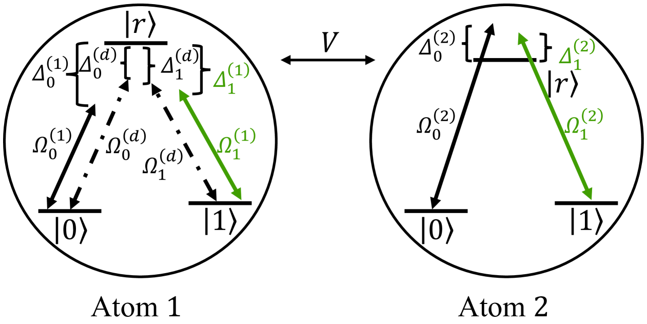
Figure 1: Sketch of two coupled Rydberg atoms under largely-detuned driving fields. $V$ represents the Rydberg interaction between them. Each Rydberg atom consists of two ground states $|0\rangle$ and $|1\rangle$ and one Rydberg state $|r\rangle$.

Consider two coupled Rydberg atoms under driving fields as shown in Fig. 1. The atom consists of two stable low-energy states $|0\rangle$ and $|1\rangle$ and one Rydberg state $|r\rangle$. The first atom and the second one are driven by the red-detuned and blue-detuned laser fields, respectively, with time-dependent Rabi frequencies $\Omega_{0,1}^{(j)}(t)$ and time-independent detuning $\Delta_{0,1}^{(j)}$, $j=1,2$. In addition, the transitions $|r\rangle\leftrightarrow|n\rangle$, $n=0,1$, of the first atom have two extra driving fields with Rabi frequency $\Omega_{n}^{(d)}(t)$ and detuning $\Delta_{n}^{(d)}$. The full Hamiltonian in the rotating frame with respect to the free Hamiltonian of the two atoms can be written as

$$H(t)=\left[H_{1}(t)+H_{d}(t)\right]\otimes\mathcal{I}_{2}+\mathcal{I}_{1}\otimes H_{2}(t)+V|rr\rangle\langle rr|,$$ (28)

with

$$H_{1}(t)=\sum_{n=0}^{1}\Omega_{n}^{(1)}(t)e^{i\Delta_{n}^{(1)}t}|r\rangle_{1}\langle n|+{\rm H.c.},$$ (29)

$$H_{2}(t)=\sum_{n=0}^{1}\Omega_{n}^{(2)}(t)e^{-i\Delta_{n}^{(2)}t}|r\rangle_{2}\langle n|+{\rm H.c.},$$

$$H_{d}(t)=\sum_{n=0}^{1}\Omega_{n}^{(d)}(t)e^{i\Delta_{n}^{(d)}t}|r\rangle_{1}\langle n|+{\rm H.c.},$$

where the Hamiltonian $H_{1}(t)$ and $H_{d}(t)$ describe the driving fields on the first atom and $H_{2}(t)$ acts on the second one. Here $\mathcal{I}$ denotes the identity operator. Conventional Rydberg-blockade protocols Müller et al. (2011); Goerz et al. (2014); Müller et al. (2014); Møller et al. (2008); Rao and Mølmer (2014); Levine et al. (2019); Graham et al. (2019) take advantage of the substantial energy shift for the operator $|rr\rangle\langle rr|$ Walker and Saffman (2008) induced by the strong vdW coupling by the last term in Eq. (28). However, realizing strong Rydberg interaction necessitates exciting the atoms to the high-lying Rydberg states and maintains the atoms in close proximity. It could have a significant and undesirable fluctuation in coupling strength Robicheaux et al. (2021). In contrast, we use the detunings of driving fields to compensate a much weaker Rydberg interaction.

In the second-rotated frame with respect to $\mathcal{U}(t)=\exp(-iVt|rr\rangle\langle rr|)$, the Hamiltonian in Eq. (28) can be transformed as

$$H_{I}(t)=H_{R}(t)+H_{D}(t)$$ (30)

with

$$H_{R}(t)=\sum_{n=0}^{1}\Omega_{n}^{(1)}(t)e^{i\Delta_{n}^{(1)}t}(|r0\rangle\langle n0|+|r1\rangle\langle n1|$$ (31)

$$+e^{iVt}|rr\rangle\langle nr|)+\sum_{n=0}^{1}\Omega_{n}^{(2)}(t)e^{-i\Delta_{n}^{(2)}t}(|0r\rangle\langle 0n|$$

$$+|1r\rangle\langle 1n|+e^{iVt}|rr\rangle\langle rn|)+{\rm H.c.},$$

and

$$H_{D}(t)=\sum_{n=0}^{1}\Omega_{n}^{(d)}(t)e^{i\Delta_{n}^{(d)}t}(|r0\rangle\langle n0|+|r1\rangle\langle n1|$$ (32)

$$+e^{iVt}|rr\rangle\langle nr|)+{\rm H.c.},$$

where $H_{D}(t)$ is used to distinguish the extra driving on the first atom. The transition diagram in the whole Hilbert space is demonstrated in Fig. 2(a).

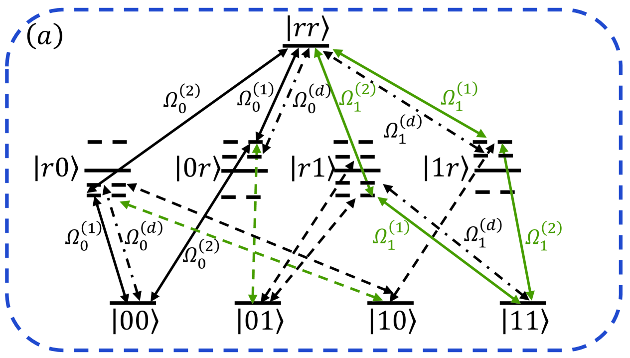
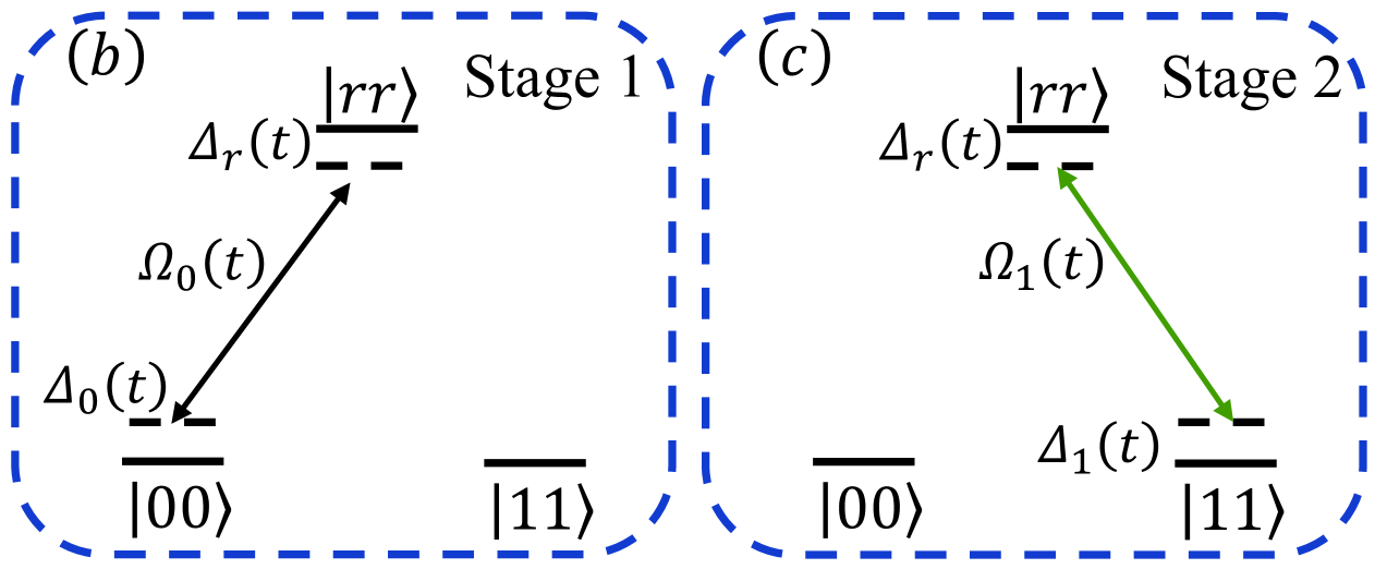
Figure 2: (a) Transition diagram for the two Rydberg atomic system driven by largely-detuned driving fields. The black and green solid lines describe the effective transitions $|rr\rangle\leftrightarrow|00\rangle$ (Stage 1) with coupling strength $\Omega_{0}(t)$ and $|rr\rangle\leftrightarrow|11\rangle$ (Stage 2) with coupling strength $\Omega_{1}(t)$, respectively. The round trips plotted with dotted-dashed lines contribute to the effective detunings $\Delta_{0}(t)$, $\Delta_{r}(t)$, and $\Delta_{1}(t)$ for the states $|00\rangle$, $|rr\rangle$, and $|11\rangle$. The transitions indicated by the black and green dashed lines can be strongly suppressed under large detunings, i.e., $\Delta_{n}^{(j)}\gg\Omega_{n}^{(j)}$, $n=0,1$. (b) and (c) Effective transition diagram in the three-dimensional subspace for Stage 1 and Stage 2, respectively.

The following protocol for generate a double-excitation Bell state with the ground levels of the Rydberg system assumes a large detuning for all the fields, i.e., $\Delta_{n}^{(j)}\gg\Omega_{n}^{(j)}(t)$ and $\Delta_{n}^{(d)}\gg\Omega_{n}^{(d)}(t)$. It consists of two stages, which are assumed to have the same period $T$.

Stage 1.— On this stage, the two-atom system is forced to evolve from the ground state $|00\rangle$ to the superposed state $(|00\rangle+|rr\rangle)/\sqrt{2}$. By switching on (off) the driving fields on the transition $|r\rangle\leftrightarrow|0\rangle$ ($|r\rangle\leftrightarrow|1\rangle$) of both atoms, the control Hamiltonian in Eq. (30) is reduced to

$$H_{I}(t)=\Omega_{0}^{(1)}(t)e^{i\Delta_{0}^{(1)}t}(|r0\rangle\langle 00|+|r1\rangle\langle 01|$$ (33)

$$+e^{iVt}|rr\rangle\langle 0r|)+\Omega_{0}^{(2)}(t)e^{-i\Delta_{0}^{(2)}t}(|0r\rangle\langle 00|+|1r\rangle\langle 10|$$

$$+e^{iVt}|rr\rangle\langle r0|)+\Omega_{0}^{(d)}(t)e^{i\Delta_{0}^{(d)}t}(|r0\rangle\langle 00|+|r1\rangle\langle 01|$$

$$+e^{iVt}|rr\rangle\langle 0r|)+{\rm H.c.}.$$

With the setting that $\Delta_{0}^{(1)}+V=\Delta_{0}^{(2)}$ and $\Omega_{0}^{(1)}(t)=\Omega_{0}^{(2)}(t)$, the effective Hamiltonian can be obtained as

$$H_{\rm eff}(t) =\Delta_{r}(t)|rr\rangle\langle rr|+\Delta_{0}(t)|00\rangle\langle 00|$$ (34)

$$+\Omega_{0}(t)|rr\rangle\langle 00|+{\rm H.c.}$$

according to Eq. (12). Here the effective detunings $\Delta_{0}(t)$ and $\Delta_{r}(t)$ and Rabi-frequency $\Omega_{0}(t)$ are

$$\Delta_{r}(t)=\frac{[\Omega_{0}^{(d)}(t)]^{2}}{\Delta_{0}^{(d)}+V},\quad\Delta_{0}(t)=-\frac{[\Omega_{0}^{(d)}(t)]^{2}}{\Delta_{0}^{(d)}}\approx-\Delta_{r}(t),$$ (35)

$$\Omega_{0}(t)=[\Omega_{0}^{(1)}(t)]^{2}\left[\frac{1}{\Delta_{0}^{(2)}}-\frac{1}{\Delta_{0}^{(1)}}\right],$$

where the approximation holds under the condition of $\Delta_{0}^{(d)}\gg V$. Then the transition diagram in Fig. 2(a) is reduced to that in Fig. 2(b).

Equivalently we are left with a two-level system in the subspace spanned by $|00\rangle$ and $|rr\rangle$, in which the energy splitting $2\Delta_{r}(t)$ and the transition rate $\Omega_{0}(t)$ can be manipulated by the driving intensities $\Omega_{0}^{(d)}(t)$ and $\Omega_{0}^{(1)}(t)$, respectively. Applying the universal control theory in Sec. II.2, the system dynamics can be described by the ancillary basis states Jin and Jing (2025a, b). They can be written as

$$|\mu_{1}(t)\rangle =\cos\theta(t)e^{i\frac{\alpha(t)}{2}}|00\rangle-\sin\theta(t)e^{-i\frac{\alpha(t)}{2}}|rr\rangle,$$ (36)

$$|\mu_{2}(t)\rangle =\sin\theta(t)e^{i\frac{\alpha(t)}{2}}|00\rangle+\cos\theta(t)e^{-i\frac{\alpha(t)}{2}}|rr\rangle,$$

where the parameters $\theta(t)$ and $\alpha(t)$ can be used to control the population and the relative phase between the states $|00\rangle$ and $|rr\rangle$, respectively.

Substitute the ancillary basis states in Eq. (36) into the von Neumann equation (21) with the effective Hamiltonian in Eq. (34), we have

$$2\Delta_{r}(t)=\dot{\alpha}(t)+2\Omega_{0}(t)\cot 2\theta(t)\cos\alpha(t),$$ (37)

$$\Omega_{0}(t)=-\frac{\dot{\theta}(t)}{\sin\alpha(t)}.$$

Due to Eq. (20), the time-evolution operator reads,

$$U(t,0)=e^{if(t)}|\mu_{1}(t)\rangle\langle\mu_{1}(0)|+e^{-if(t)}|\mu_{2}(t)\rangle\langle\mu_{2}(0)|,$$ (38)

where the global phase satisfies

$$\dot{f}(t)=\Omega_{0}(t)\frac{\cos\alpha(t)}{\sin 2\theta(t)}=-\dot{\theta}(t)\frac{\cot\alpha(t)}{\sin 2\theta(t)}.$$ (39)

Taking $\theta(t)$, $\alpha(t)$ and $f(t)$ as independent variables, the conditions in Eq. (37) can be expressed as

$$2\Delta_{r}(t)=\dot{\alpha}(t)+2\dot{f}(t)\cos 2\theta(t),$$ (40a)

$$\Omega_{0}(t)=-\sqrt{\dot{\theta}(t)^{2}+\dot{f}(t)^{2}\sin^{2}2\theta(t)},$$ (40b)

$$\dot{\alpha}(t)=-\frac{\ddot{\theta}\dot{f}\sin 2\theta-\ddot{f}\dot{\theta}\sin 2\theta-2\ddot{f}\dot{\theta}^{2}\cos 2\theta}{\dot{f}^{2}\sin^{2}2\theta+\dot{\theta}^{2}}.$$ (40c)

With Eqs. (35) and (40), the Rabi-frequencies $\Omega_{0}^{(1)}(t)$ and $\Omega_{0}^{(d)}(t)$ in the lab can be practically formulated as

$$\Omega_{0}^{(1)}(t) =\sqrt{\Omega_{0}(t)\left[\Delta_{0}^{(1)}\Delta_{0}^{(2)}\right]/\left[\Delta_{0}^{(2)}-\Delta_{0}^{(1)}\right]},$$ (41)

$$\Omega_{0}^{(d)}(t) =\sqrt{\Delta_{r}(t)\Delta_{0}^{(d)}}.$$

The quantum task of Stage 1 can thus be accomplished by selecting either passage $|\mu_{1}(t)\rangle$ or $|\mu_{2}(t)\rangle$ in Eq. (36), through appropriate setting of the parameters $\theta(t)$, $\alpha(t)$, and $f(t)$. For example, when $\theta(0)=0$, $\alpha(0)=0$, $\theta(T)=\pi/4$, and $\alpha(T)=\pi$, where $T$ is the effective evolution period, the state $|00\rangle$ can evolve to $(|00\rangle+|rr\rangle)/\sqrt{2}$ along the passage $|\mu_{1}(t)\rangle$ when $t=T$.

Stage 2.— On this stage, we target to push the system from the superposed state $(|00\rangle+|rr\rangle)/\sqrt{2}$ to the double-excitation Bell state encoded with the ground states $|00\rangle$ and $|11\rangle$. On the contrary to Stage 1, now we switch on (off) the driving fields on the transition $|r\rangle\leftrightarrow|1\rangle$ ($|r\rangle\leftrightarrow|0\rangle$) of both atoms. The rotated Hamiltonian in Eq. (30) is then reduced to

$$H_{I}(t)=\Omega_{1}^{(1)}(t)e^{i\Delta_{1}^{(1)}t}(|r0\rangle\langle 10|+|r1\rangle\langle 11|$$ (42)

$$+e^{iVt}|rr\rangle\langle 1r|)+\Omega_{1}^{(2)}(t)e^{-i\Delta_{1}^{(2)}t}(|0r\rangle\langle 01|+|1r\rangle\langle 11|$$

$$+e^{iVt}|rr\rangle\langle r1|)+\Omega_{1}^{(d)}(t)e^{i\Delta_{1}^{(d)}t}(|r0\rangle\langle 10|+|r1\rangle\langle 11|$$

$$+e^{iVt}|rr\rangle\langle 1r|)+{\rm H.c.}.$$

Similar to Stage 1, the detunings and Rabi frequencies are set as $\Delta_{1}^{(1)}+V=\Delta_{1}^{(2)}$ and $\Omega_{1}^{(1)}(t)=\Omega_{1}^{(2)}(t)$, then the effective Hamiltonian becomes

$$H_{\rm eff}(t) =\Delta_{r}(t)|rr\rangle\langle rr|+\Delta_{1}(t)|11\rangle\langle 11|$$ (43)

$$+\Omega_{1}(t)|rr\rangle\langle 11|+{\rm H.c.},$$

where

$$\Delta_{r}(t)=\frac{[\Omega_{1}^{(d)}(t)]^{2}}{\Delta_{1}^{(d)}+V},\quad\Delta_{1}(t)=-\frac{[\Omega_{1}^{(d)}(t)]^{2}}{\Delta_{1}^{(d)}}\approx-\Delta_{r}(t),$$ (44)

$$\Omega_{1}(t)=[\Omega_{1}^{(1)}(t)]^{2}\left[\frac{1}{\Delta_{1}^{(2)}}-\frac{1}{\Delta_{1}^{(1)}}\right].$$

Consequently, the transition diagram in Fig. 2(a) is reduced to that in Fig. 2(c), in which the ground state $|00\rangle$ is decoupled from the system dynamics on this stage. Similar to Eq. (36), the dynamics under parametric control can be described by the ancillary basis states superposed by $|11\rangle$ and $|rr\rangle$:

$$|\mu_{1}(t)\rangle =\cos\theta(t)e^{i\frac{\alpha(t)}{2}}|11\rangle-\sin\theta(t)e^{-i\frac{\alpha(t)}{2}}|rr\rangle,$$ (45)

$$|\mu_{2}(t)\rangle =\sin\theta(t)e^{i\frac{\alpha(t)}{2}}|11\rangle+\cos\theta(t)e^{-i\frac{\alpha(t)}{2}}|rr\rangle.$$

Replacing $\Omega_{0}(t)$ in Eqs. (37), (39), and (40) with $\Omega_{1}(t)$, one can again obtain the same time-evolution operator in Eq. (38) if the Rabi frequencies $\Omega_{1}^{(1)}(t)$ and $\Omega_{1}^{(d)}(t)$ satisfy the same conditions in Eq. (41) for $\Omega_{0}^{(1)}(t)$ and $\Omega_{0}^{(d)}(t)$, respectively. Under the boundary conditions that $\theta(T+0^{+})=\pi/2$, $\theta(2T)=0$, and $\alpha(T+0^{+})=\alpha(2T)=\pi$, the system can evolve from $(|00\rangle+|rr\rangle)/\sqrt{2}$ for $t=T$ to $(|00\rangle+\exp[if(2T)]|11\rangle)/\sqrt{2}$ along $|\mu_{1}(t)\rangle$ when $t=2T$.

III.2 Nonideal situation and numerical calculation

In this section, we first examine the robustness of our protocol against the environmental noises, and then apply the correction mechanism in Eq. (27) to suppress the adverse effects induced from the systematic errors.

Without loss of generality, the parameter $\theta(t)$ for both stages [in Eqs. (36) and (45)] can be set as

$$\theta(t)=\left\{\begin{aligned} &\frac{\pi t}{4T},\quad t\in\left[0,T\right]\\ &\frac{\pi t}{2T},\quad t\in\left[T,2T\right]\end{aligned}\right.$$ (46)

We use the Lindblad master equation to take account the environmental noise into account Carmichael (1999), which reads,

$$\frac{\partial\rho}{\partial t}=-i[H(t),\rho]+\sum_{j=1}^{2}\left[\frac{\kappa_{0}}{2}\mathcal{L}(|0\rangle_{j}\langle r|)+\frac{\kappa_{1}}{2}\mathcal{L}(|1\rangle_{j}\langle r|)\right].$$ (47)

Here $\rho$ is the density matrix for the two coupled Rydberg atoms, $H(t)$ is the full Hamiltonian in Eq. (28), and $\mathcal{L}(o)$ is the Lindblad superoperator defined as $\mathcal{L}(o)\equiv 2o\rho o^{\dagger}-o^{\dagger}o\rho-\rho o^{\dagger}o$ Scully and Zubairy (1997). Particularly, $|0\rangle_{j}\langle r|$ and $|1\rangle_{j}\langle r|$ represent the spontaneous emission of the $j$th atom from its Rydberg state $|r\rangle$ to the ground states $|0\rangle$ and $|1\rangle$ with decay rates $\kappa_{0}$ and $\kappa_{1}$, respectively. For simplicity, we assume $\kappa_{0}=\kappa_{1}=\kappa/2$. The decoherence rate $\kappa$ for the Rydberg states of the alkali-metal atoms Beterov et al. (2009); Isenhower et al. (2010); Adams et al. (2020) with a low angular momentum relates to the principle and azimuthal quantum numbers Adams et al. (2020), which is typically in the range of $0.75\sim 2.48$ kHz Beterov et al. (2009); Isenhower et al. (2010) around the room temperature.

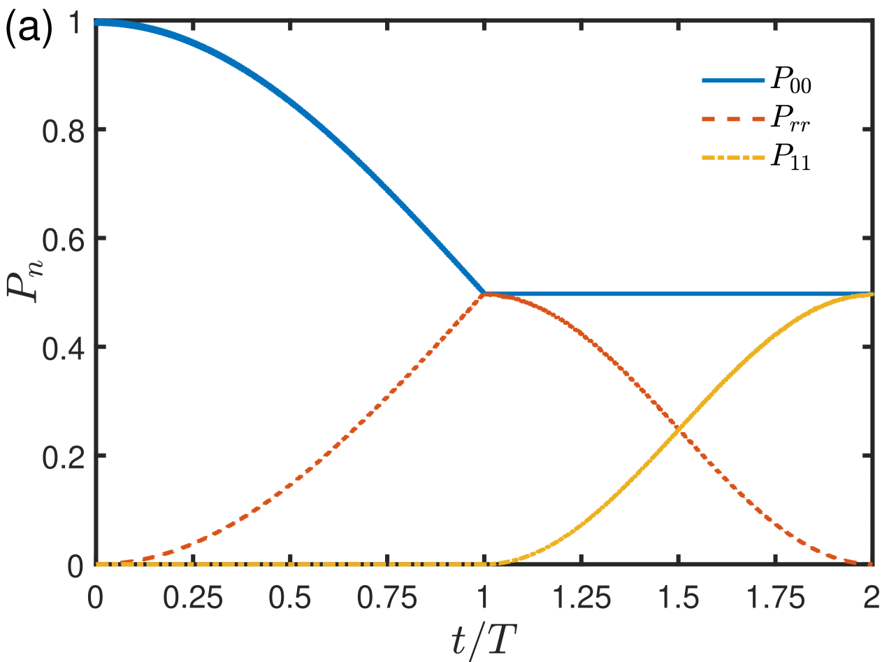
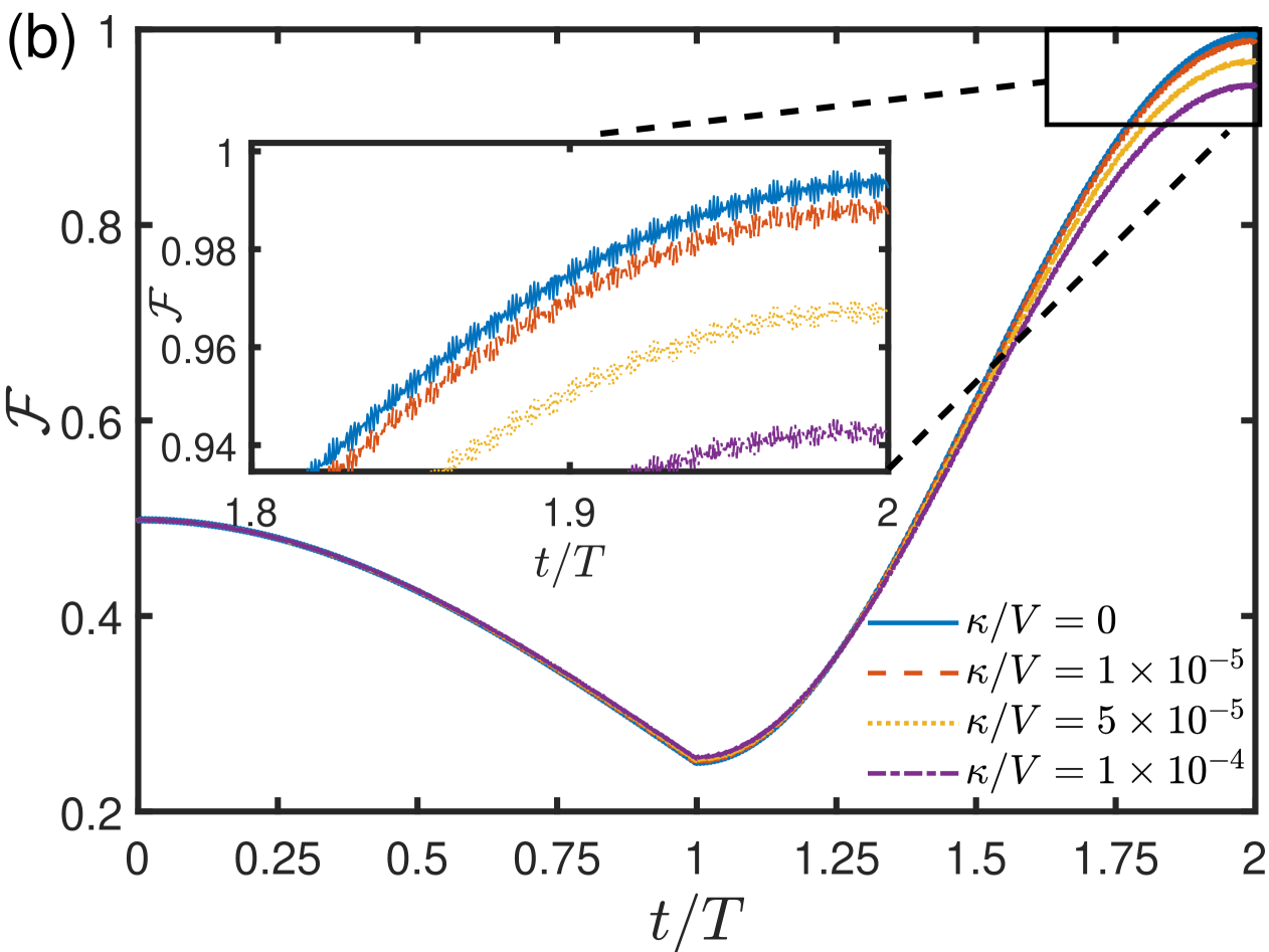
Figure 3: (a) Population dynamics $P_{n}$, $n=00,rr,11$, for the decoherence-free system and (b) Fidelity dynamics $\mathcal{F}$ for the target state $(|00\rangle+|11\rangle)/\sqrt{2}$ for both closed and open systems. The period for each stage is set as $T=1\mu$s. The detunings in the lab are set as $\Delta_{n}^{(1)}=10V$, $\Delta_{n}^{(2)}=\Delta_{n}^{(1)}+V$, and $\Delta_{n}^{(d)}=5V$, with $n=0,1$ and $V/2\pi=200$ MHz. The Rabi frequencies in the lab are maintained as $\Omega_{0}^{(1)}(t)=\Omega_{0}^{(2)}(t)$ (Stage 1) and $\Omega_{1}^{(1)}(t)=\Omega_{1}^{(2)}(t)$ (Stage 2), where $\Omega_{0}^{(1)}(t)$ and $\Omega_{1}^{(1)}(t)$ are obtained by Eq. (41). The effective detuning $\Delta_{r}(t)$ in Eq. (40a), the Rabi-frequencies $\Omega_{0}(t)$ (Stage 1) and $\Omega_{1}(t)$ (Stage 2) in Eq. (40b), and the phase $\alpha(t)$ in Eq. (40c) are under the conditions of $\theta(t)$ in Eq. (46) and $f(t)=0$.

The performance of our protocol can be evaluated by the state population $P_{n}=|\langle n|\rho(t)|n\rangle|$, $n=00,rr,11$, and the fidelity for the target state $|\psi_{\rm tar}\rangle=(|00\rangle+|11\rangle)/\sqrt{2}$. The fidelity is defined as $\mathcal{F}(t)={\rm Tr}[\rho_{s}^{2}(t)]$, where $\rho_{s}(t)=\Pi\rho(t)\Pi$ with $\Pi\equiv|00\rangle\langle 00|+|11\rangle\langle 11|$. Figure 3(a) demonstrates the dynamics of system populations $P_{n}$ for the closed system. During the first stage, i.e., $t\in[0,T]$, the initial state $|00\rangle$ can gradually evolve to the superposed state which equally populates the states $|00\rangle$ and $|rr\rangle$. Then, during the second stage $t\in[T,2T]$, the population on the Rydberg state $|rr\rangle$ can be completely transferred to the ground state $|11\rangle$ and the population on $|00\rangle$ is untouched. In Fig. 3(b), the dynamics of fidelity $\mathcal{F}$ about the Bell state $|\psi_{\rm tar}\rangle=(|00\rangle+|11\rangle)/\sqrt{2}$ is demonstrated under various decay rates $\kappa$. In the ideal situation, i.e., $\kappa=0$, the fidelity is about $\mathcal{F}(2T)=0.995$ on account of the leakage to the whole Hilbert space. Our protocol presents a robust performance when the system is exposed to a dissipative environment. Under an experimentally practical decay rate, i.e., $\kappa/V=1\times 10^{-5}$ ($\kappa/2\pi\sim 2$ kHz), the final fidelity is still as high as $\mathcal{F}(2T)=0.987$. Even when $\kappa/V=1\times 10^{-4}$, which is about $10$ times as high as the practical one, $\mathcal{F}(2T)=0.969$. In the conventional protocols based on Rydberg blockade Jaksch et al. (2000); Levine et al. (2019); Graham et al. (2019); Møller et al. (2008) and asymmetric blockade Brion et al. (2007); Saffman and Mølmer (2009); Wu et al. (2010); Rao and Mølmer (2014); Young et al. (2021), the Rydberg interaction $V$ is required to two orders higher than the Rabi frequencies. In our protocol, the ratio of Rydberg interaction to Rabi frequency can be as low as $V/\Omega_{0}^{(1)}(t)\sim 5$, as determined by the parametric setting in Fig. 3.

In the presence of the systematical errors, the original Hamiltonian in Eq. (28) will be perturbed as

$$H(t)\rightarrow H(t)+H_{e}(t),$$ (48)

where $H_{e}(t)$ is the error Hamiltonian. Without loss of generality, it can be categorized to the global error

$$H_{e}(t)=\epsilon\left[H_{1}(t)+H_{d}(t)\right]\otimes\mathcal{I}_{2}+\epsilon\mathcal{I}_{1}\otimes H_{2}(t),$$ (49)

and the local error

$$H_{e}(t)=\epsilon\left[H_{1}(t)+H_{d}(t)\right]\otimes\mathcal{I}_{2}.$$ (50)

They describe the global fluctuation of the driving fields on both atoms and the individual fluctuation of the driving fields on the first atom, respectively. By Eq. (35), it is found that the global and local errors yield different consequence to the effective Hamiltonian (34) for Stage 1. They read,

$$H_{\rm eff}^{\prime}(t) =(1+\epsilon)^{2}\Big{[}\Delta_{r}(t)|rr\rangle\langle rr|+\Delta_{0}(t)|00\rangle\langle 00|$$ (51)

$$+\Omega_{0}(t)|rr\rangle\langle 00|+{\rm H.c.}\Big{]},$$

and

$$H_{\rm eff}^{\prime}(t) =(1+\epsilon)^{2}\Big{[}\Delta_{r}(t)|rr\rangle\langle rr|+\Delta_{0}(t)|00\rangle\langle 00|\Big{]}$$ (52)

$$+(1+\epsilon)\Big{[}\Omega_{0}(t)|rr\rangle\langle 00|+{\rm H.c.}\Big{]},$$

respectively. Similarly, the effective Hamiltonian (43) for Stage 2 become Eqs. (51) and (52) under global and local errors, respectively, with $|00\rangle\rightarrow|11\rangle$, $\Omega_{0}\rightarrow\Omega_{1}$, and $\Delta_{0}\rightarrow\Delta_{1}$.

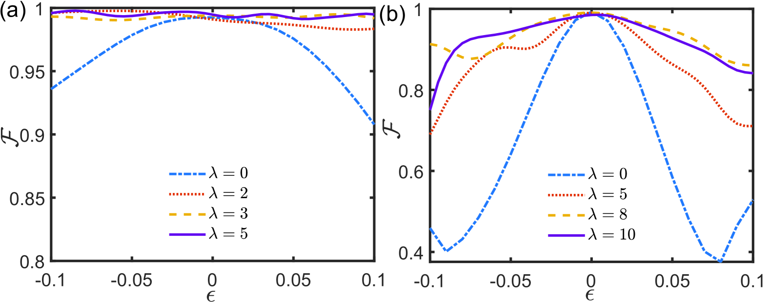
Figure 4: Fidelity $\mathcal{F}(2T)$ about the target Bell state $(|00\rangle+\exp[if(2T)]|11\rangle)/\sqrt{2}$ versus the error magnitude $\epsilon$ with (a) the global error and (b) the local error for both stages under various control magnitudes $\lambda$ in Eq. (53). $\kappa=0$. The other parameters are the same as Fig. 3.

In our model, a simple solution for the correction mechanism (27) is to set the global phase as

$$\dot{f}(t)=\lambda\dot{\theta}(t),$$ (53)

where $\dot{\theta}(t)$ can be used to estimate the evolution and transition rates of the universal passages in Eqs. (36) and (45). The adverse effects induced by small errors can be suppressed as long as $\lambda$ is sufficiently large, that is shown in Fig. 4 about the final fidelity for the target state $(|00\rangle+\exp[if(2T)]|11\rangle)/\sqrt{2}$ with a nonvanishing local phase. Under the global error, Fig. 4(a) demonstrates that for $\lambda=0$ (with no correction), the fidelity decreases to $\mathcal{F}(2T)=0.936$ when $\epsilon=-0.1$, $\mathcal{F}(2T)=0.979$ when $\epsilon=-0.05$, $\mathcal{F}(2T)=0.976$ when $\epsilon=0.05$, and $\mathcal{F}(2T)=0.908$ when $\epsilon=0.1$. With correction, the passage exhibits a less susceptibility to the global error. It becomes $\mathcal{F}(2T)>0.983$ when $\lambda=2$, $\mathcal{F}(2T)>0.991$ when $\lambda=3$, and $\mathcal{F}(2T)>0.993$ when $\lambda=5$, over the whole range of $\epsilon\in[-0.1,0.1]$. Figure 4(b) demonstrates the results under the local errors, which are more harmful than the global error. For $\lambda=0$ (with no correction), the fidelity will be as low as $\mathcal{F}(2T)=0.641$ when $\epsilon=-0.05$ and $\mathcal{F}(2T)=0.595$ when $\epsilon=0.05$. A larger $\lambda$ than that in case of the global error is required to hold the nonadiabatic passage. Over the range of $\epsilon\in[-0.05,0.05]$, the fidelity improves to $\mathcal{F}>0.863$ when $\lambda=5$ and $\mathcal{F}>0.928$ when $\lambda=8$.

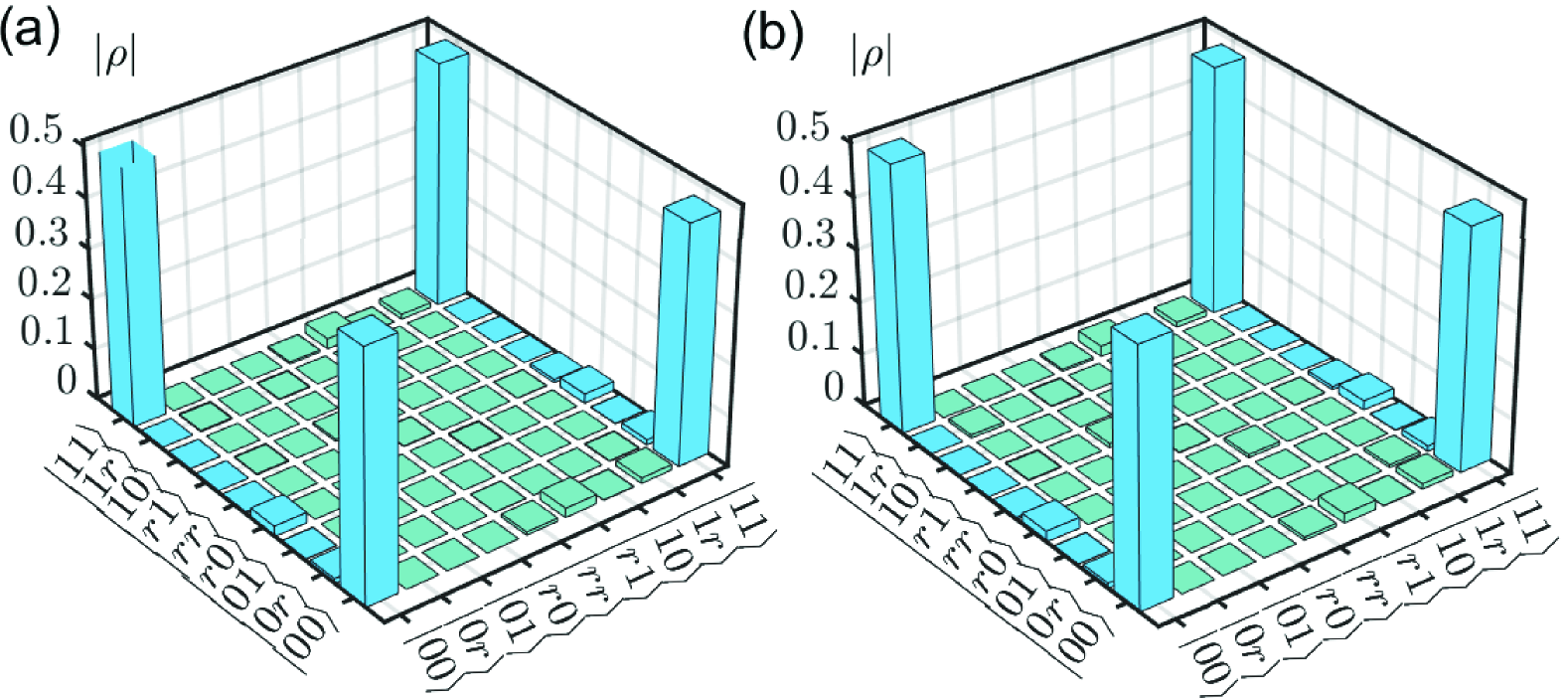
Figure 5: Absolute value of density matrix of the atomic system $|\rho(t=2T)|$ under the global error in Eq. (49) with $\epsilon=-0.1$. The control coefficient in Eq. (53) is set as $\lambda=5$. The decay rate is $\kappa/V=1\times 10^{-5}$ in (a) and $\kappa/V=5\times 10^{-5}$ in (b). The other parameters are set the same as Fig. 3.

Figure 5 shows the final density matrix $|\rho(t=2T)|$ for the open atomic system in the presence of both environmental noise and global error in Hamiltonian. $|\rho|$ means taking the absolute value for each element of the $9\times 9$ density matrix of the two Rydberg atoms. In Fig. 5(a) with $\kappa/V=1\times 10^{-5}$, the numerical calculation demonstrates that $|\langle 00|\rho(2T)|11\rangle|=0.492$, $|\langle 00|\rho(2T)|00\rangle|=0.512$, and $|\langle 11|\rho(2T)|11\rangle|=0.472$. The fidelity is found to be $\mathcal{F}(2T)=0.984$ on account of the leakage to the Rydberg state $|r\rangle$. In Fig. 5(b) with a much larger decay rate, the matrix elements are found to be $|\langle 00|\rho(2T)|11\rangle|=0.475$, $|\langle 00|\rho(2T)|00\rangle|=0.504$, and $|\langle 11|\rho(2T)|11\rangle|=0.448$. The fidelity is about $\mathcal{F}(2T)=0.951$. Thus our protocol with error correction shows remarkable performance in comparison to the ideal-parameter case in Fig. 3, even under deviations of a $10\%$ level in parameter. These results also show the insensitive of our protocol to the environmental noise.

IV Maximally entangling multiple qubits via robust universal passages

In this section, our protocol is extended to prepare a general GHZ state of $N$ Rydberg atoms that are coupled through the nearest-neighboring Rydberg interaction, i.e., $H_{\rm int}=V\sum_{k=1}^{N-1}|rr\rangle_{k,k+1}\langle rr|$. The protocol is completed within $N-1$ steps, the $k$th step of which, $1\leq k\leq N-1$, is characterized by only driving the $k$th and $(k+1)$th Rydberg atoms with largely detuned laser fields. Initially, the whole system is assumed to be at the ground state $|0\rangle^{\otimes N}$.

Step 1. The atom-pair under driving has exactly the same configuration space as that in Fig. 1. Following the same process as the two-atom case in Sec. III.1, this step is divided into two stages with equal duration $T$. On Stage 1, the atomic system evolves from the ground state $|0\rangle^{\otimes N}$ to the superposed state $(|00\rangle+|rr\rangle)\otimes|0\rangle^{\otimes(N-2)}/\sqrt{2}$. On Stage 2, it is prepared to be the state equally superposed by the ground states $|0\rangle^{\otimes N}$ and $|11\rangle\otimes|0\rangle^{\otimes(N-2)}$. The only distinction is that the passages for these two stages [see Eqs. (36) and (45)] become

$$|\mu_{1}(t)\rangle =\Big{[}\cos\theta(t)e^{i\frac{\alpha(t)}{2}}|00\rangle$$ (54)

$$-\sin\theta(t)e^{-i\frac{\alpha(t)}{2}}|rr\rangle\Big{]}\otimes|0\rangle^{\otimes(N-2)},$$

$$|\mu_{2}(t)\rangle =\Big{[}\sin\theta(t)e^{i\frac{\alpha(t)}{2}}|00\rangle$$

$$+\cos\theta(t)e^{-i\frac{\alpha(t)}{2}}|rr\rangle\Big{]}\otimes|0\rangle^{\otimes(N-2)},$$

and

$$|\mu_{1}(t)\rangle =\Big{[}\cos\theta(t)e^{i\frac{\alpha(t)}{2}}|rr\rangle$$ (55)

$$-\sin\theta(t)e^{-i\frac{\alpha(t)}{2}}|11\rangle\Big{]}\otimes|0\rangle^{\otimes(N-2)},$$

$$|\mu_{2}(t)\rangle =\Big{[}\sin\theta(t)e^{i\frac{\alpha(t)}{2}}|rr\rangle$$

$$+\cos\theta(t)e^{-i\frac{\alpha(t)}{2}}|11\rangle\Big{]}\otimes|0\rangle^{\otimes(N-2)},$$

respectively.

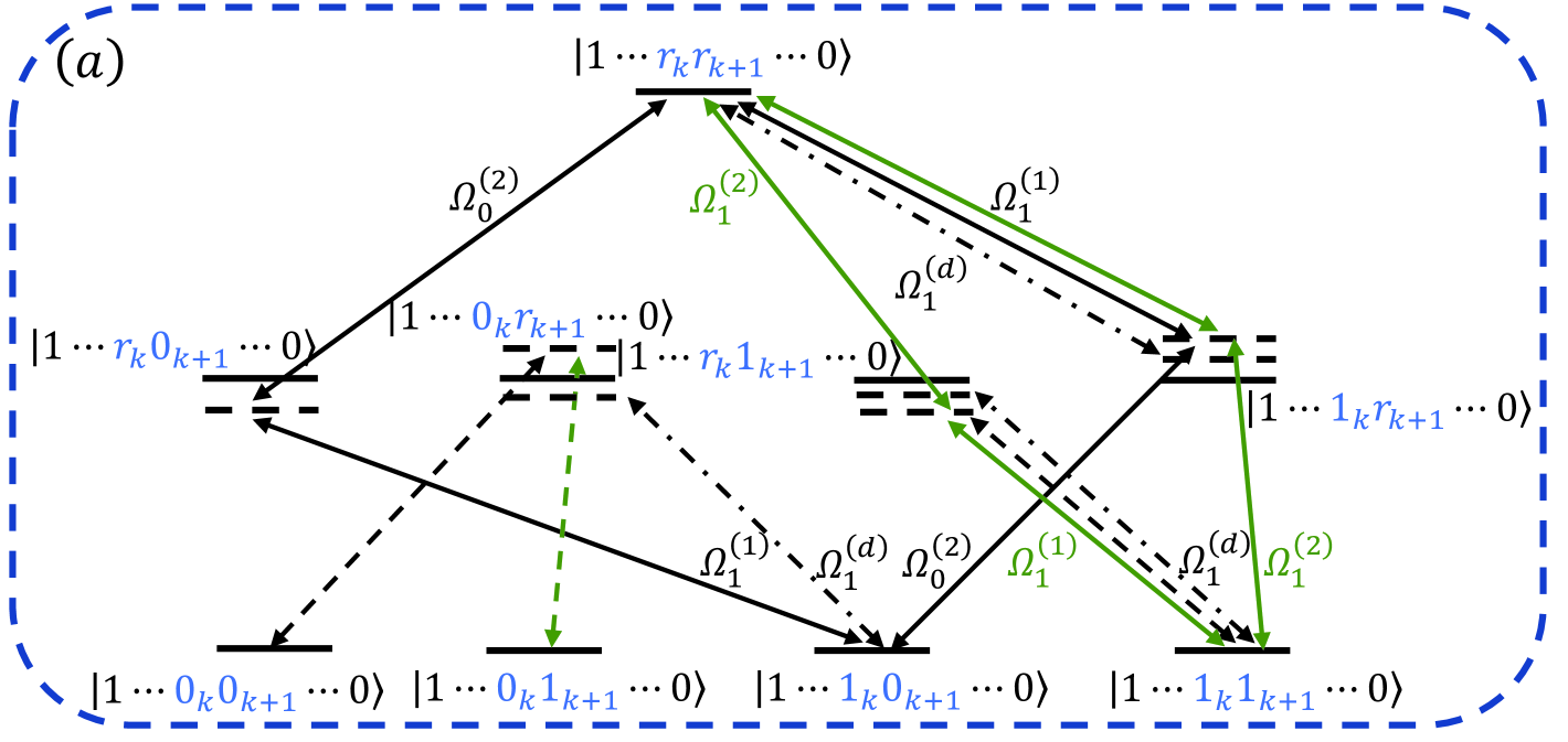
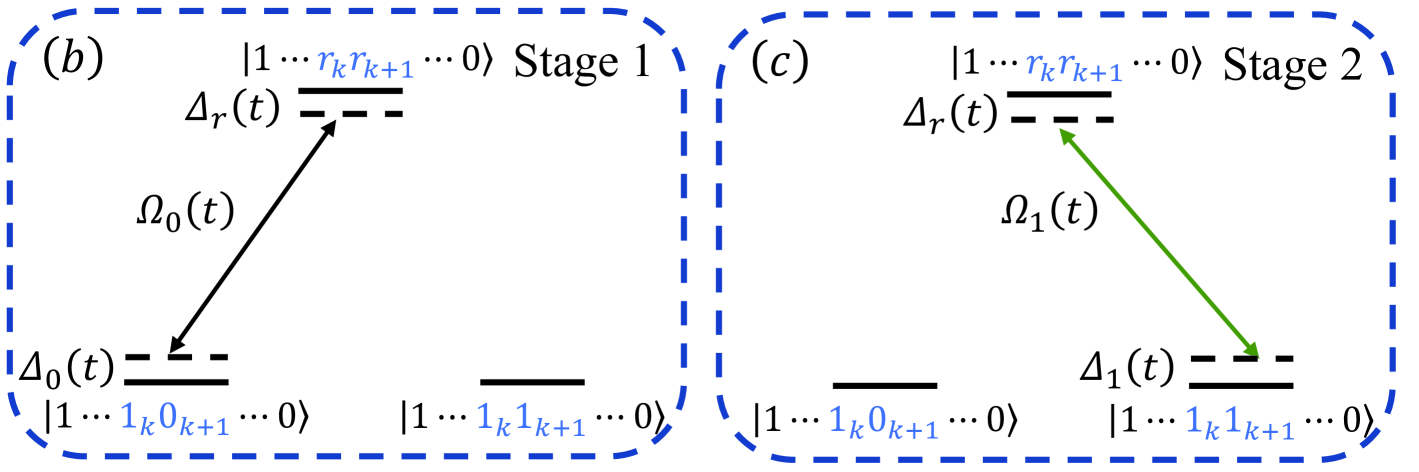
Figure 6: (a) Transition diagram for the multiple Rydberg atomic system driven by largely-detuned driving fields in the $k$th step. The black and green solid lines describe the effective transitions $|1\cdots r_{k}r_{k+1}\cdots 0\rangle\leftrightarrow|1\cdots 1_{k}0_{k+1}\cdots 0\rangle$ (Stage 1) with coupling strength $\Omega_{0}(t)$ and $|1\cdots r_{k}r_{k+1}\cdots 0\rangle\leftrightarrow|1\cdots 1_{k}1_{k+1}\cdots 0\rangle$ (Stage 2) with coupling strength $\Omega_{1}(t)$, respectively. The round trips plotted with dotted-dashed lines contribute to the effective detunings $\Delta_{0}(t)$, $\Delta_{r}(t)$, and $\Delta_{1}(t)$ for the states $|1\cdots 1_{k}0_{k+1}\cdots 0\rangle$, $|1\cdots r_{k}r_{k+1}\cdots 0\rangle$, and $|1\cdots 1_{k}1_{k+1}\cdots 0\rangle$. The transitions indicated by the black and green dashed lines can be strongly suppressed under large detunings, i.e., $\Delta_{n}^{(j)}\gg\Omega_{n}^{(j)}$, $n=0,1$. (b) and (c) Effective transition diagrams in the three-dimensional subspace for Stage 1 and Stage 2, respectively.

Step $k$, $2\leq k\leq N-1$. Regarding the first and the second atoms in Fig. 1 as the $k$th and the $k+1$th atoms in this step, respectively, their configuration under driving is slightly different from that in Fig. 1 by switching off the driving fields for the transition $|r\rangle\leftrightarrow|0\rangle$ in the $k$th atom, i.e., $\Omega_{0}^{(1)}(t)=0$ and $\Omega_{0}^{(d)}(t)=0$. Consequently, the rotated Hamiltonian $H_{I}(t)$ (30) is modified to be

$$H_{I}(t)=\Omega_{1}^{(1)}(t)e^{i\Delta_{1}^{(1)}t}(|r0\rangle_{k,k+1}\langle 10|+|r1\rangle_{k,k+1}\langle 11|$$ (56)

$$+e^{iVt}|rr\rangle_{k,k+1}\langle 1r|)+\sum_{n=0}^{1}\Omega_{n}^{(2)}(t)e^{-i\Delta_{n}^{(2)}t}(|0r\rangle_{k,k+1}\langle 0n|$$

$$+|1r\rangle_{k,k+1}\langle 1n|+e^{iVt}|rr\rangle_{k,k+1}\langle rn|)+\Omega_{1}^{(d)}(t)e^{i\Delta_{1}^{(d)}t}\times$$

$$(|r0\rangle_{k,k+1}\langle 10|+|r1\rangle_{k,k+1}\langle 11|+e^{iVt}|rr\rangle_{k,k+1}\langle 1r|)+{\rm H.c.}$$

Therefore, the transition diagram in Fig. 2(a) becomes Fig. 6(a) within the subspace spanned by the states where the atoms $k^{\prime}<k$ are in the state $|1\rangle$, and the atoms $k^{\prime}>k+1$ are in the state $|0\rangle$.

Note now one half of population remains on the ground state $|0\rangle^{\otimes N}$ throughout all the steps $k>1$, as it is decoupled from the system dynamics. Each step also consists of two stages with equal duration $T$. On Stage 1, the population on $|1\cdots 1_{k}0_{k+1}\cdots 0\rangle$ is transferred to $|1\cdots r_{k}r_{k+1}\cdots 0\rangle$, where the subscript $k$ indexes the $k$th atom. Then on Stage 2, the population on $|1\cdots r_{k}r_{k+1}\cdots 0\rangle$ is transferred to $|1\cdots 1_{k}1_{k+1}\cdots 0\rangle$. Thus a general $N$-qubits GHZ state, i.e., the state equally superposed by the ground states $|0\rangle^{\otimes N}$ and $|1\rangle^{\otimes N}$, can be prepared at the end of the $(N-1)$th step.

In particular, on Stage 1, i.e., $t\in[2(k-1)T,(2k-1)T]$, the driving field on the transition $|r\rangle\leftrightarrow|1\rangle$ of the $(k+1)$th atom is switched off, and the other driving fields satisfy the conditions of $\Delta_{1}^{(1)}+V=\Delta_{0}^{(2)}$ and $\Omega_{1}^{(1)}(t)=\Omega_{0}^{(2)}(t)$. Using Eq. (12) and the modified $H_{I}(t)$ in Eq. (56), the effective Hamiltonian can be obtained as

$$H_{\rm eff}(t) =\Delta_{r}(t)|rr\rangle_{k,k+1}\langle rr|+\Delta_{0}(t)|10\rangle_{k,k+1}\langle 10|$$ (57)

$$+\Omega_{0}(t)|rr\rangle_{k,k+1}\langle 10|+{\rm H.c.},$$

where $\Delta_{r}(t)$, $\Delta_{0}(t)$, and $\Omega_{0}(t)$ follow the similar formations as in Eq. (35) under the substitutions $\Omega_{0}^{(d)}(t)\rightarrow\Omega_{1}^{(d)}(t)$, $\Delta_{0}^{(d)}(t)\rightarrow\Delta_{1}^{(d)}(t)$, $\Omega_{0}^{(1)}(t)\rightarrow\Omega_{1}^{(1)}(t)$, and $\Delta_{0}^{(1)}(t)\rightarrow\Delta_{1}^{(1)}(t)$. Then the transition diagram for the subspace in Fig. 6(a) can be reduced to that in Fig. 6(b). Following Eqs. (36), (45), (54), and (55), the ancillary basis states for Fig. 6(b) can be chosen as

$$|\mu_{1}(t)\rangle=|1\rangle^{\otimes(k-1)}\otimes\Big{[}\cos\theta(t)e^{i\frac{\alpha(t)}{2}}|10\rangle$$ (58)

$$-\sin\theta(t)e^{-i\frac{\alpha(t)}{2}}|rr\rangle\Big{]}\otimes|0\rangle^{\otimes(N-k-1)},$$

$$|\mu_{2}(t)\rangle=|1\rangle^{\otimes(k-1)}\otimes\Big{[}\sin\theta(t)e^{i\frac{\alpha(t)}{2}}|10\rangle$$

$$+\cos\theta(t)e^{-i\frac{\alpha(t)}{2}}|rr\rangle\Big{]}\otimes|0\rangle^{\otimes(N-k-1)},$$

When $\Delta_{r}(t)$ and $\Omega_{0}(t)$ in Eq. (57) satisfy the conditions in Eqs. (37) or (40) with $\theta[2(k-1)T+0^{+}]=0$ and $\theta[(2k-1)T]=\pi/2$, the population on the state $|1\cdots 1_{k}0_{k+1}\cdots 0\rangle$ can be completely transferred to the state $|1\cdots r_{k}r_{k+1}\cdots 0\rangle$ along the passage $|\mu_{1}(t)\rangle$ when $t=(2k-1)T$.

On Stage 2, i.e., $t\in[(2k-1)T,2kT]$, we switch off the driving field on the transition $|r\rangle\leftrightarrow|0\rangle$ of the $(k+1)$th atom and tune the other driving fields to satisfy the conditions of $\Delta_{1}^{(1)}+V=\Delta_{1}^{(2)}$ and $\Omega_{1}^{(1)}(t)=\Omega_{1}^{(2)}(t)$. Then we achieve the same effective Hamiltonian as in Eq. (43) only with a different pair of atoms:

$$H_{\rm eff}(t) =\Delta_{r}(t)|rr\rangle_{k,k+1}\langle rr|+\Delta_{1}(t)|11\rangle_{k,k+1}\langle 11|$$ (59)

$$+\Omega_{1}(t)|rr\rangle_{k,k+1}\langle 11|+{\rm H.c.},$$

where $\Delta_{r}(t)$, $\Delta_{1}(t)$, and $\Omega_{1}(t)$ adopt the same conditions in Eq. (44). Then the transition diagram in Fig. 6(a) reduces to that in Fig. 6(c). Similar to Eqs. (36), (45), (54), (55) and (58), the ancillary basis states for Fig. 6(c) can be chosen as

$$|\mu_{1}(t)\rangle=|1\rangle^{\otimes(k-1)}\otimes\Big{[}\cos\theta(t)e^{i\frac{\alpha(t)}{2}}|rr\rangle$$ (60)

$$-\sin\theta(t)e^{-i\frac{\alpha(t)}{2}}|11\rangle\Big{]}\otimes|0\rangle^{\otimes(N-k-1)},$$

$$|\mu_{2}(t)\rangle=|1\rangle^{\otimes(k-1)}\otimes\Big{[}\sin\theta(t)e^{i\frac{\alpha(t)}{2}}|rr\rangle$$

$$+\cos\theta(t)e^{-i\frac{\alpha(t)}{2}}|11\rangle\Big{]}\otimes|0\rangle^{\otimes(N-k-1)}.$$

Under the conditions in Eqs. (37) or (40) with the substitution of $\Omega_{1}(t)$ for $\Omega_{0}(t)$, the population on $|1\cdots r_{k}r_{k+1}\cdots 0\rangle$ can be transferred to $|1\cdots 1_{k}1_{k+1}\cdots 0\rangle$ along the passage $|\mu_{2}(t)\rangle$ when $t=2kT$, for the boundary conditions $\theta[(2k-1)T]=\pi/2$ and $\theta(2kT)=\pi$. Thus one can set $\theta(t)=\pi[t-2(k-1)T]/(2T)$ for $k>1$. When $N-1$ steps are completed, the whole system is prepared as a general GHZ state.

Table 1: Fidelity $\mathcal{F}$ about the target $N$-qubit GHZ state encoded with the ground states for the open systems with no correction. The Rabi frequency and detuning are in the order of $\gamma$, where $\gamma\equiv 2\pi\times 1$ MHz is an energy unit.

$\kappa/\gamma$	$N=2$	$N=3$	$N=4$	$N=5$	$N=6$	$N=7$
$1\times 10^{-3}$	0.999	$0.999$	$0.999$	$0.998$	$0.998$	$0.997$
$5\times 10^{-3}$	0.998	$0.995$	$0.993$	$0.990$	$0.988$	$0.986$
$1\times 10^{-2}$	0.996	$0.991$	$0.986$	$0.981$	$0.976$	$0.971$

In Tab. 1, we present the fidelity $\mathcal{F}$ of $N$-qubit GHZ state for the open systems. With no correction, the target state reads $[|0\rangle^{\otimes N}+(-1)^{N-1}|1\rangle^{\otimes N}]/\sqrt{2}$. The dynamics of the multiple Rydberg atomic system is described by the master equation,

$$\frac{\partial\rho}{\partial t}=-i[H_{\rm eff}(t),\rho]+\frac{\kappa}{2}\sum_{k=1}^{N}\left[\mathcal{L}(|0\rangle_{k}\langle r|)+\mathcal{L}(|1\rangle_{k}\langle r|)\right],$$ (61)

where $H_{\rm eff}(t)$ can be selected from Eqs. (33), (42), (57), and (59) in the relevant stages of evolution. And the fidelity is obtained in the retained encoded subspace spanned by the ground states $|0\rangle$ and $|1\rangle$. Again the results justify that our protocol is not sensitive to the environmental noise. Under the practical decay-rate $\kappa/\gamma=1\times 10^{-3}$, the fidelity is found to be about $\mathcal{F}=0.999$ when $N=3$ and $N=4$, $\mathcal{F}=0.998$ when $N=5$ and $N=6$, and $\mathcal{F}=0.997$ when $N=7$. When the decay rate is as large as $\kappa/\gamma=1\times 10^{-2}$ (10 times as the practical one), the fidelity is about $\mathcal{F}=0.991$ for $N=3$, $\mathcal{F}=0.986$ for $N=4$, $\mathcal{F}=0.981$ for $N=5$, $\mathcal{F}=0.976$ for $N=6$, and $\mathcal{F}=0.971$ when $N=7$.

We also check the performance of our error-correction mechanism (27) against the systematic errors, e.g., in the preparation of the general GHZ state of six Rydberg atoms, i.e., $[|0\rangle^{\otimes 6}+\exp[i\sum_{k=2}^{6}f(2kT)]|1\rangle^{\otimes 6}]/\sqrt{2}$. In the presence of the global error about the driving fields on both atoms, i.e., $\Omega_{n}^{(j)}(t)\rightarrow(1+\epsilon)\Omega_{n}^{(j)}(t)$ with $n=0,1$, the effective Hamiltonian fluctuates as $H_{\rm eff}(t)\rightarrow(1+\epsilon)^{2}H_{\rm eff}(t)$ due to Eq. (51). With a significant error $\epsilon=-0.1$ and the identical setting of the other parameters, it is found that the target-state fidelities become almost the same as those in Tab. 1 as long as the control coefficient $\lambda\geq 5$ in Eq. (53).

V Conclusion and discussion

In summary, we designed a protocol of state generation under the universal quantum control framework to prepare a high-fidelity $N$-qubit GHZ state encoded with the hyperfine ground states of the Rydberg atoms. The protocol is performed along the universal nonadiabatic passages using largely detuned driving fields, which avoids the conventional requirement about the strong Rydberg interaction in the generation of Bell state Levine et al. (2018); Madjarov et al. (2020). Our protocol shows robustness against the environmental noise for the target state does not involve with the sensitive Rydberg state. In addition, a passage-dependent and rapid-varying global phase can be used to counteract the systematic errors.

Our protocol is superior to the existing protocols implemented with trapped-ion Monz et al. (2011) and superconducting systems Zhong et al. (2021) in both scalability and reliability. The former is due to the vanishing crosstalk among atoms out of a small radius, while the latter relies on the long lifetime of the single unit of the multipartite entangled state. The coherent time of the hyperfine ground states of Rydberg atoms is typically of the order of second Wang et al. (2016); Sheng et al. (2018), which surpasses that of trapped ions ($\sim$ms) Monz et al. (2011) and that of superconducting qubits ($\sim\mu$s) Zhong et al. (2021) by orders of magnitude. Our protocol therefore provides a powerful tool to generate a high-fidelity maximally entangled states in neutral atomic systems for quantum information process and quantum computation.

References

- Král et al. (2007) P. Král, I. Thanopulos, and M. Shapiro, Colloquium: Coherently controlled adiabatic passage, Rev. Mod. Phys. 79, 53 (2007).
- Li (2020) W. Li, A boost to rydberg quantum computing, Nat. Phys. 16, 820 (2020).
- Einstein et al. (1935) A. Einstein, B. Podolsky, and N. Rosen, Can quantum-mechanical description of physical reality be considered complete? Phys. Rev. 47, 777 (1935).
- Bohr (1935) N. Bohr, Can quantum-mechanical description of physical reality be considered complete? Phys. Rev. 48, 696 (1935).
- Horodecki et al. (2009) R. Horodecki, P. Horodecki, M. Horodecki, and K. Horodecki, Quantum entanglement, Rev. Mod. Phys. 81, 865 (2009).
- Ekert and Jozsa (1996) A. Ekert and R. Jozsa, Quantum computation and shor’s factoring algorithm, Rev. Mod. Phys. 68, 733 (1996).
- Farhi et al. (2001) E. Farhi, J. Goldstone, S. Gutmann, J. Lapan, A. Lundgren, and D. Preda, A quantum adiabatic evolution algorithm applied to random instances of an np-complete problem, Science 292, 472 (2001).
- Bravyi et al. (2018) S. Bravyi, D. Gosset, and R. König, Quantum advantage with shallow circuits, Science 362, 308 (2018).
- Bennett et al. (1993) C. H. Bennett, G. Brassard, C. Crépeau, R. Jozsa, A. Peres, and W. K. Wootters, Teleporting an unknown quantum state via dual classical and einstein-podolsky-rosen channels, Phys. Rev. Lett. 70, 1895 (1993).
- Raussendorf and Briegel (2001) R. Raussendorf and H. J. Briegel, A one-way quantum computer, Phys. Rev. Lett. 86, 5188 (2001).
- Gidney and Ekerå (2019) C. Gidney and M. Ekerå, How to factor 2048 bit rsa integers in 8 hours using 20 million noisy qubits, Quantum 5, 433 (2019).
- Ladd et al. (2010) T. D. Ladd, F. Jelezko, R. Laflamme, Y. Nakamura, C. Monroe, and J. L. O’Brien, Quantum computers, Nature 464, 45 (2010).
- Benhelm et al. (2008) J. Benhelm, G. Kirchmair, C. F. Roos, and R. Blatt, Towards fault-tolerant quantum computing with trapped ions, Nat. Phys. 4, 463 (2008).
- Monz et al. (2011) T. Monz, P. Schindler, J. T. Barreiro, M. Chwalla, D. Nigg, W. A. Coish, M. Harlander, W. Hänsel, M. Hennrich, and R. Blatt, 14-qubit entanglement: Creation and coherence, Phys. Rev. Lett. 106, 130506 (2011).
- Harty et al. (2014) T. P. Harty, D. T. C. Allcock, C. J. Ballance, L. Guidoni, H. A. Janacek, N. M. Linke, D. N. Stacey, and D. M. Lucas, High-fidelity preparation, gates, memory, and readout of a trapped-ion quantum bit, Phys. Rev. Lett. 113, 220501 (2014).
- Ballance et al. (2016) C. J. Ballance, T. P. Harty, N. M. Linke, M. A. Sepiol, and D. M. Lucas, High-fidelity quantum logic gates using trapped-ion hyperfine qubits, Phys. Rev. Lett. 117, 060504 (2016).
- Gaebler et al. (2016) J. P. Gaebler, T. R. Tan, Y. Lin, Y. Wan, R. Bowler, A. C. Keith, S. Glancy, K. Coakley, E. Knill, D. Leibfried, and D. J. Wineland, High-fidelity universal gate set for ion qubits, Phys. Rev. Lett. 117, 060505 (2016).
- Chow et al. (2012) J. M. Chow, J. M. Gambetta, A. D. Córcoles, S. T. Merkel, J. A. Smolin, C. Rigetti, S. Poletto, G. A. Keefe, M. B. Rothwell, J. R. Rozen, M. B. Ketchen, and M. Steffen, Universal quantum gate set approaching fault-tolerant thresholds with superconducting qubits, Phys. Rev. Lett. 109, 060501 (2012).
- Barends et al. (2014a) R. Barends, J. Kelly, A. Megrant, A. Veitia, D. Sank, E. Jeffrey, T. C. White, J. Mutus, A. G. Fowler, B. Campbell, Y. Chen, Z. Chen, B. Chiaro, A. Dunsworth, C. Neill, P. O’Malley, P. Roushan, A. Vainsencher, J. Wenner, A. N. Korotkov, A. N. Cleland, and J. M. Martinis, Superconducting quantum circuits at the surface code threshold for fault tolerance, Nature 508, 500 (2014a).
- Song et al. (2019) C. Song, K. Xu, H. Li, Y.-R. Zhang, X. Zhang, W. Liu, Q. Guo, Z. Wang, W. Ren, J. Hao, H. Feng, H. Fan, D. Zheng, D.-W. Wang, H. Wang, and S.-Y. Zhu, Generation of multicomponent atomic schrödinger cat states of up to 20 qubits, Science 365, 574 (2019).
- Wright et al. (2019) K. Wright, K. M. Beck, S. Debnath, J. M. Amini, Y. Nam, N. Grzesiak, J.-S. Chen, N. C. Pisenti, M. Chmielewski, C. Collins, K. M. Hudek, J. Mizrahi, J. D. Wong-Campos, S. Allen, J. Apisdorf, P. Solomon, M. Williams, A. M. Ducore, A. Blinov, S. M. Kreikemeier, V. Chaplin, M. Keesan, C. Monroe, and J. Kim, Benchmarking an 11-qubit quantum computer, Nat. Commun. 10, 5464 (2019).
- Barends et al. (2014b) R. Barends, J. Kelly, A. Megrant, A. Veitia, D. Sank, E. Jeffrey, T. C. White, J. Mutus, A. G. Fowler, B. Campbell, Y. Chen, Z. Chen, B. Chiaro, A. Dunsworth, C. Neill, P. O’Malley, P. Roushan, A. Vainsencher, J. Wenner, A. N. Korotkov, A. N. Cleland, and J. M. Martinis, Superconducting quantum circuits at the surface code threshold for fault tolerance, Nature 508, 500 (2014b).
- Zhong et al. (2021) Y. Zhong, H.-S. Chang, A. Bienfait, E. Dumur, M.-H. Chou, C. R. Conner, J. Grebel, R. G. Povey, H. Yan, D. I. Schuster, and A. N. Cleland, Deterministic multi-qubit entanglement in a quantum network, Nature 590, 571 (2021).
- Saffman et al. (2010) M. Saffman, T. G. Walker, and K. Mølmer, Quantum information with rydberg atoms, Rev. Mod. Phys. 82, 2313 (2010).
- Xia et al. (2015) T. Xia, M. Lichtman, K. Maller, A. W. Carr, M. J. Piotrowicz, L. Isenhower, and M. Saffman, Randomized benchmarking of single-qubit gates in a 2d array of neutral-atom qubits, Phys. Rev. Lett. 114, 100503 (2015).
- Wang et al. (2016) Y. Wang, A. Kumar, T.-Y. Wu, and D. S. Weiss, Single-qubit gates based on targeted phase shifts in a 3d neutral atom array, Science 352, 1562 (2016).
- Sheng et al. (2018) C. Sheng, X. He, P. Xu, R. Guo, K. Wang, Z. Xiong, M. Liu, J. Wang, and M. Zhan, High-fidelity single-qubit gates on neutral atoms in a two-dimensional magic-intensity optical dipole trap array, Phys. Rev. Lett. 121, 240501 (2018).
- Weiss and Saffman (2017) D. S. Weiss and M. Saffman, Quantum computing with neutral atoms, Phys. Today 70, 44 (2017).
- Levine et al. (2018) H. Levine, A. Keesling, A. Omran, H. Bernien, S. Schwartz, A. S. Zibrov, M. Endres, M. Greiner, V. Vuletić, and M. D. Lukin, High-fidelity control and entanglement of rydberg-atom qubits, Phys. Rev. Lett. 121, 123603 (2018).
- Madjarov et al. (2020) I. S. Madjarov, J. P. Covey, A. L. Shaw, J. Choi, A. Kale, A. Cooper, H. Pichler, V. Schkolnik, J. R. Williams, and M. Endres, High-fidelity entanglement and detection of alkaline-earth rydberg atoms, Nat. Phys. 16, 857 (2020).
- Omran et al. (2019) A. Omran, H. Levine, A. Keesling, G. Semeghini, T. T. Wang, S. Ebadi, H. Bernien, A. S. Zibrov, H. Pichler, S. Choi, J. Cui, M. Rossignolo, P. Rembold, S. Montangero, T. Calarco, M. Endres, M. Greiner, V. Vuletić, and M. D. Lukin, Generation and manipulation of schrödinger cat states in rydberg atom arrays, Science 365, 570 (2019).
- Barredo et al. (2016) D. Barredo, S. de Léséleuc, V. Lienhard, T. Lahaye, and A. Browaeys, An atom-by-atom assembler of defect-free arbitrary two-dimensional atomic arrays, Science 354, 1021 (2016).
- Ebadi et al. (2021) S. Ebadi, T. T. Wang, H. Levine, A. Keesling, G. Semeghini, A. Omran, D. Bluvstein, R. Samajdar, H. Pichler, W. W. Ho, S. Choi, S. Sachdev, M. Greiner, V. Vuletić, and M. D. Lukin, Quantum phases of matter on a 256-atom programmable quantum simulator, Nature 595, 227 (2021).
- Barredo et al. (2018) D. Barredo, V. Lienhard, S. de Léséleuc, T. Lahaye, and A. Browaeys, Synthetic three-dimensional atomic structures assembled atom by atom, Nature 561, 79 (2018).
- Barredo et al. (2020) D. Barredo, V. Lienhard, P. Scholl, S. de Léséleuc, T. Boulier, A. Browaeys, and T. Lahaye, Three-dimensional trapping of individual rydberg atoms in ponderomotive bottle beam traps, Phys. Rev. Lett. 124, 023201 (2020).
- Browaeys et al. (2016) A. Browaeys, D. Barredo, and T. Lahaye, Experimental investigations of dipole–dipole interactions between a few rydberg atoms, J. Phys. B: At., Mol. Opt. Phys. 49, 152001 (2016).
- Walker and Saffman (2008) T. G. Walker and M. Saffman, Consequences of zeeman degeneracy for the van der waals blockade between rydberg atoms, Phys. Rev. A 77, 032723 (2008).
- Jaksch et al. (2000) D. Jaksch, J. I. Cirac, P. Zoller, S. L. Rolston, R. Côté, and M. D. Lukin, Fast quantum gates for neutral atoms, Phys. Rev. Lett. 85, 2208 (2000).
- Levine et al. (2019) H. Levine, A. Keesling, G. Semeghini, A. Omran, T. T. Wang, S. Ebadi, H. Bernien, M. Greiner, V. Vuletić, H. Pichler, and M. D. Lukin, Parallel implementation of high-fidelity multiqubit gates with neutral atoms, Phys. Rev. Lett. 123, 170503 (2019).
- Graham et al. (2019) T. M. Graham, M. Kwon, B. Grinkemeyer, Z. Marra, X. Jiang, M. T. Lichtman, Y. Sun, M. Ebert, and M. Saffman, Rydberg-mediated entanglement in a two-dimensional neutral atom qubit array, Phys. Rev. Lett. 123, 230501 (2019).
- Møller et al. (2008) D. Møller, L. B. Madsen, and K. Mølmer, Quantum gates and multiparticle entanglement by rydberg excitation blockade and adiabatic passage, Phys. Rev. Lett. 100, 170504 (2008).
- Brion et al. (2007) E. Brion, A. S. Mouritzen, and K. Mølmer, Conditional dynamics induced by new configurations for rydberg dipole-dipole interactions, Phys. Rev. A 76, 022334 (2007).
- Saffman and Mølmer (2009) M. Saffman and K. Mølmer, Efficient multiparticle entanglement via asymmetric rydberg blockade, Phys. Rev. Lett. 102, 240502 (2009).
- Wu et al. (2010) H.-Z. Wu, Z.-B. Yang, and S.-B. Zheng, Implementation of a multiqubit quantum phase gate in a neutral atomic ensemble via the asymmetric rydberg blockade, Phys. Rev. A 82, 034307 (2010).
- Rao and Mølmer (2014) D. D. B. Rao and K. Mølmer, Deterministic entanglement of rydberg ensembles by engineered dissipation, Phys. Rev. A 90, 062319 (2014).
- Young et al. (2021) J. T. Young, P. Bienias, R. Belyansky, A. M. Kaufman, and A. V. Gorshkov, Asymmetric blockade and multiqubit gates via dipole-dipole interactions, Phys. Rev. Lett. 127, 120501 (2021).
- Robicheaux et al. (2021) F. Robicheaux, T. M. Graham, and M. Saffman, Photon-recoil and laser-focusing limits to rydberg gate fidelity, Phys. Rev. A 103, 022424 (2021).
- Pohl and Berman (2009) T. Pohl and P. R. Berman, Breaking the dipole blockade: Nearly resonant dipole interactions in few-atom systems, Phys. Rev. Lett. 102, 013004 (2009).
- Urban et al. (2009) E. Urban, T. A. Johnson, T. Henage, L. Isenhower, D. D. Yavuz, T. G. Walker, and M. Saffman, Observation of rydberg blockade between two atoms, Nat. Phys. 5, 110 (2009).
- Jin and Jing (2025a) Z.-y. Jin and J. Jing, Universal perspective on nonadiabatic quantum control, Phys. Rev. A 111, 012406 (2025a).
- Jin and Jing (2025b) Z.-y. Jin and J. Jing, Entangling distant systems via universal nonadiabatic passage, Phys. Rev. A 111, 022628 (2025b).
- Jin and Jing (2025c) Z.-y. Jin and J. Jing, Universal quantum control with error correction, arXiv: 2502, 19786 (2025c).
- James and Jerke (2007) D. F. James and J. Jerke, Effective hamiltonian theory and its applications in quantum information, Can. J. Phys. 85, 625 (2007).
- Blanes et al. (2009) S. Blanes, F. Casas, J. Oteo, and J. Ros, The magnus expansion and some of its applications, Phys. Rep. 470, 151 (2009).
- Jing et al. (2013) J. Jing, L.-A. Wu, J. Q. You, and T. Yu, Nonperturbative quantum dynamical decoupling, Phys. Rev. A 88, 022333 (2013).
- Jing et al. (2015) J. Jing, L.-A. Wu, M. Byrd, J. Q. You, T. Yu, and Z.-M. Wang, Nonperturbative leakage elimination operators and control of a three-level system, Phys. Rev. Lett. 114, 190502 (2015).
- Vitanov et al. (2017) N. V. Vitanov, A. A. Rangelov, B. W. Shore, and K. Bergmann, Stimulated raman adiabatic passage in physics, chemistry, and beyond, Rev. Mod. Phys. 89, 015006 (2017).
- Müller et al. (2011) M. M. Müller, D. M. Reich, M. Murphy, H. Yuan, J. Vala, K. B. Whaley, T. Calarco, and C. P. Koch, Optimizing entangling quantum gates for physical systems, Phys. Rev. A 84, 042315 (2011).
- Goerz et al. (2014) M. H. Goerz, E. J. Halperin, J. M. Aytac, C. P. Koch, and K. B. Whaley, Robustness of high-fidelity rydberg gates with single-site addressability, Phys. Rev. A 90, 032329 (2014).
- Müller et al. (2014) M. M. Müller, M. Murphy, S. Montangero, T. Calarco, P. Grangier, and A. Browaeys, Implementation of an experimentally feasible controlled-phase gate on two blockaded rydberg atoms, Phys. Rev. A 89, 032334 (2014).
- Carmichael (1999) H. Carmichael, Statistical Methods in Quantum Optics (Springer, Berlin, 1999).
- Scully and Zubairy (1997) M. O. Scully and M. S. Zubairy, Quantum Optics (Cambridge University Press, Cambridge, 1997).
- Beterov et al. (2009) I. I. Beterov, I. I. Ryabtsev, D. B. Tretyakov, and V. M. Entin, Quasiclassical calculations of blackbody-radiation-induced depopulation rates and effective lifetimes of rydberg , , and alkali-metal atoms with , Phys. Rev. A 79, 052504 (2009).
- Isenhower et al. (2010) L. Isenhower, E. Urban, X. L. Zhang, A. T. Gill, T. Henage, T. A. Johnson, T. G. Walker, and M. Saffman, Demonstration of a neutral atom controlled-not quantum gate, Phys. Rev. Lett. 104, 010503 (2010).
- Adams et al. (2020) C. S. Adams, J. D. Pritchard, and J. P. Shaffer, Rydberg atom quantum technologies, J. Phys. B: At. Mol. Opt. Phys. 53, 012002 (2020).