The Mid-sphere Cousin of the Medial Axis Transform

Abstract

The medial axis of a smoothly embedded surface in ${{\mathbb{R}}}^{3}$ consists of all points for which the Euclidean distance function on the surface has at least two minima. We generalize this notion to the mid-sphere axis, which consists of all points for which the Euclidean distance function has two interchanging saddles that swap their partners in the pairing by persistent homology. It offers a discrete-algebraic multi-scale approach to computing ridge-like structures on the surface. As a proof of concept, an algorithm that computes stair-case approximations of the mid-sphere axis is provided.

1 Introduction

In the late 1960s, Harry Blum [5] revolutionized the automated classification of shapes that typically arise in biology and related fields by suggesting the medial axis as a skeleton fit to describe amorphous blobs. The concept was introduced in the smooth setting by Federer [12, Definition 4.1 on page 432] almost a decade earlier, but his contribution was largely overlooked. Since then, the medial axis has been used as a tool in shape classification, image analysis, animation, computer graphics, and other fields that benefit from the feature-preserving simplification of unwieldy objects; see e.g. [4, 16, 18].

Given a closed surface, $M\subseteq{{\mathbb{R}}}^{3}$, the medial axis is the set of centers of spheres that touch $M$ in at least two points and do otherwise not intersect $M$. Slightly more elaborately, the medial axis transform is the same set of points paired with the radii at which the spheres touch $M$. Requiring instead that $M$ lies inside the spheres, we get an apparently less useful complementary concept, which for the purposes of this paper we refer to as the circum-sphere axis transform of $M$. We observe that there is an appealing third option: the mid-sphere axis transform, which consists of centers and radii of spheres that touch $M$ in at least two points, and for any two there is a closed curve on $M$ inside the sphere, and a closed curve on the sphere together with a filling surface both inside $M$; see Figure 1 for an illustration.

Figure 1: A mid-sphere touching an ellipsoid in two antipodal points. The vertical plane that passes through these two points intersects the ellipsoid in a curve that lies inside the sphere, and the horizontal plane that passes through the same two points intersects the sphere in a great-circle filled by a disk that both lie inside the ellipsoid.

All three axes are subsets of the symmetry set of $M$ defined as the set of centers of spheres that touch $M$ in at least two points. Compared to this “hopelessly complicated object” [6], the three axes are sparse skeleta that specialize in bringing out particular types of features. For example, the mid-sphere axis is sensitive to ridge-like features, in which a point $x\in M$ belongs to a curve called a ridge if it locally minimizes or maximizes the curvature along a principle curvature direction; see e.g. Chapter 11 on “Ridges and Ribs” in [15]. This definition is in terms of derivatives and thus hyper-sensitive to local noise. We propose that complementing it with more global topological requirements, we get more reliably computable access to ridge-like structures.

Outline. Section 2 formally defines the mid-sphere axis transform. Section 3 reviews the Morse theory of the squared distance function from a point. Section 4 introduces the notion of Faustian interchanges, which characterize the mid-sphere axis transform. Section 5 explains the pairing mechanism of persistent homology and its connection to Faustian interchanges. Section 6 exploits the vineyard algorithm to compute an approximation of the mid-sphere axis transform. Section 7 concludes the paper.

2 The Mid-sphere Axis Transform

As illustrated in Figure 2, a point may belong to the mid-sphere axis for more than one radius. In other words, the projection of the mid-sphere axis transform in ${{\mathbb{R}}}^{4}$ to the mid-sphere axis in ${{\mathbb{R}}}^{3}$ is not necessarily injective, which is in contrast to the medial and the circum-sphere axes.

Let $M\subseteq{{\mathbb{R}}}^{3}$ be a smoothly embedded connected closed surface, and write $S=S(x,r)$ for the sphere with center $x\in{{\mathbb{R}}}^{3}$ and radius $r>0$. The set ${{\mathbb{R}}}^{3}\setminus M$ consists of two open components, a bounded one called the inside of $M$, and an unbounded one called the outside of $M$. Similarly, we distinguish between the inside of $S$, which is an open ball, and the outside of $S$, which is the complement of a closed ball. The sphere touches the surface in a point $b\in M\cap S$ if the tangent planes of $M$ and $S$ at $b$ agree, and it touches $M$ generically if $\nicefrac{{1}}{{r}}$ is different from the two principal curvatures of $M$ at $b$.

\begin{picture}(5580.0,5444.0)(811.0,-4583.0)\end{picture}

Figure 2: Two locally cylindrical pieces of a blue surface with elliptic cross-sections as shown. The smaller cylinder runs inside the wider cylinder, and both share an axis normal to the drawing plane. The two yellow spheres touch the two cylinders in two points each, and because these spheres are concentric but have different radii, their center belongs to two different red sheets of the mid-sphere axis, which intersect in a line that runs along the common central axis of the two cylinders.

Definition 1

Let $M\subseteq{{\mathbb{R}}}^{3}$ be a smoothly embedded surface. A point-radius pair $(x,r)\in{{\mathbb{R}}}^{3}\times{{\mathbb{R}}}$ belongs to the mid-sphere axis transform of $M$ if

1. $S=S(x,r)$ touches $M$ generically in at least two points, $b\neq c$;

2. there is a smooth closed curve, $\mu\subseteq M$, that passes through $b$ and $c$ and lies otherwise inside $S$;

3. there is a smooth closed curve, $\sigma\subseteq S$, that passes through $b$ and $c$, and a filling surface, $\tau$, with boundary $\sigma$, that both lie otherwise inside $M$.

If $M$ is homeomorphic to a sphere, then Condition (iii) can be weakened because the existence of $\tau$ follows from the existence of $\sigma$. We write ${{\mathcal{M}id}}{({M})}$ for the mid-sphere axis transform of $M$. Generically, it is a $2$-dimensional surface in ${{\mathbb{R}}}^{4}$. The mid-sphere axis is the projection to ${{\mathbb{R}}}^{3}$ defined by forgetting the radii. This projection is not necessarily an embedding, so the mid-sphere axis can have self-intersections.

3 Morse Theory of Squared Distance Function

The interaction of the surface, $M\subseteq{{\mathbb{R}}}^{3}$, with spheres centered at $x\in{{\mathbb{R}}}^{3}$ is conveniently described using the Euclidean distance of the points on $M$ from $x$. This is a smooth function on $M$, unless $x\in M$, so it is preferable to use the square of this distance, which is always smooth. We thus introduce $f_{x}\colon M\to{{\mathbb{R}}}$ defined by $f_{x}(y)={\|{y}-{x}\|}^{2}$. Writing $\nabla f_{x}(y)$ and $H_{x}(y)$ for the gradient and the Hessian of $f_{x}$ at $y\in M$, a point $y\in M$ is a critical point of $f_{x}$ if $\nabla f_{x}(y)=0$, and it is non-degenerate if $H_{x}(y)$ is invertible. The values of critical points are called critical values of $f_{x}$, and all other values are non-critical values. Non-degenerate critical points are necessarily isolated, so if all critical points are non-degenerate, then there are only finitely many of them. Indeed, $f_{x}$ is generically a Morse function [14], which is slightly stronger and requires that $f_{x}$ satisfies two conditions:

• all critical points are non-degenerate;

• the values of the critical points are distinct.

Assuming $f_{x}\colon M\to{{\mathbb{R}}}$ is Morse, there are only three types of critical points: minima, saddles, maxima, which can be distinguished by the number of negative eigenvalues of the Hessian, which is $0$, $1$, $2$, in this sequence. This number is traditionally referred to as the index of the critical point; see Figure 3 where we see $2$ minima, $3$ saddles, and $1$ maximum of the displayed height function.

Figure 3: The six non-empty sublevel sets at non-critical values interleaved between the critical values of the height function on the torus-with-a-nose. The lowest and highest of the three saddles both give birth, while the middle saddle gives death. On the right, we see the barcode that shows for which value a gap, loop, or closed surface exists in the sublevel set (see Section 5 for definitions).

Besides the three local types, we also distinguish between two global types of critical points. For this, we write $M_{r}=f_{x}^{-1}[0,r^{2}]$ for the sublevel set of $f_{x}$ at $r^{2}$, which contains all points whose Euclidean distance from $x$ is at most $r$. A fundamental result in Morse theory [14] is that $M_{r}$ and $M_{s}$ have the same homotopy type if there is no critical values in the open interval $(r,s)$. Furthermore, whenever $(r,s)$ contains a single critical value, then $M_{r}$ and $M_{s}$ have different homotopy types. To quantify this difference, we use the ranks of the $p$-th reduced homology groups, which we denote ${{\beta}_{p}}(M_{r})$. Whenever we pass the value of a minimum, ${{\beta}_{0}}$ increases by $1$, unless this is the first minimum, in which case ${{\beta}_{-1}}$ decreases from $1$ to $0$. Whenever we pass the value of a saddle, either two components merge, in which case ${{\beta}_{0}}$ decreases by $1$, or a component gains a loop, in which case ${{\beta}_{1}}$ increases by $1$. Finally, whenever we pass the value of a maximum, ${{\beta}_{1}}$ decreases by $1$, unless this is the last maximum, in which case ${{\beta}_{2}}$ increases from $0$ to $1$. This exhausts all cases and we note that each non-degenerate critical point changes only one rank by $1$. We say the critical point gives birth if the rank increases by $1$, and it gives death if the rank decreases by $1$.

Both the local and the global types of the critical points of the squared distance function will be important to determine whether a point, $x$, with associated radius, $r$ belongs to the mid-sphere axis transform.

4 Faustian Interchanges

Consider now a continuous $1$-parameter family (a curve) of smooth functions that starts with a Morse function on $M$ and ends with another Morse function on $M$. Unless these two Morse functions are very similar, the family necessarily passes through functions that are not Morse. By the essential property of Cerf theory [7], it is possible to choose the family such that it passes through only a finite number of functions that are not Morse, and each such function has only one violation of the two conditions that characterize a smooth function as Morse:

1. two critical points that share the same value;

2. one degenerate critical point with simple local neighborhood.

A violation II is the transient configuration that appears when two critical points collide and in the process annihilate each other. We refer to it as a cancellation of the two critical points. Its inverse is an anti-cancellation, which creates two critical points where there were none. We are however more interested in a violation I, which is the transient configuration that appears when two critical points swap the order of their values. We refer to it as an interchange.

An interchange of two minima does not affect their global type, unless they are the first two minima (the ones with smallest value). Then the first minimum becomes second and changes from giving death to giving birth, and the other way around for the second minimum. This happens where the curve of squared distance functions crosses the medial axis, because the point at the crossing has two closest points on $M$ or, equivalently, the squared distance function from the crossing has two minima with smallest value.

Definition 2

A Faustian interchange is an interchange of two critical points during which they swap their global types, one from giving death to giving birth and other from giving birth to giving death.

Critical points that swap their global types when they interchange necessarily have the same index; see Section 5. As described above, the Faustian interchanges of two minima correspond to points of the medial axis, and by a similar argument, the Faustian interchanges of two maxima correspond to points of the circum-sphere axis. Most important for this paper are the Faustian interchanges of two saddles, which correspond to points of the mid-sphere axis.

Theorem 4.1

A point $x\in{{\mathbb{R}}}^{3}$ with radius $r>0$ belongs to the mid-sphere axis transform of $F$ iff $f_{x}$ has a Faustian interchange of two saddles at $r^{2}$.

Proof

“$\implies$”: Assuming $(x,r)\in{{\mathcal{M}id}}{({M})}$, let $b,c\in M$ be the points at which $S=S(x,r)$ touches $M$, and let $\mu,\sigma$ be the two closed curves and $\tau$ the surface that fills $\sigma$ whose existence is guaranteed by Conditions (ii) and (iii) of Definition 1. Let $X$ be the connected component of $M_{r}$ that contains $b$ and $c$. The connectivity of $X\setminus\{b\}$ and $X\setminus\{c\}$ is clear from the existence of $\mu$. It is also clear that $b$ and $c$ cannot be minima or maxima, so they are saddles. If $X\setminus\{b,c\}$ is connected, then there is a curve that starts at one branch of $\mu\setminus\{b,c\}$ and ends at the other whose points lie on or inside $S$. But this curve contradicts the existence of the curve $\sigma$ and the surface $\tau$ that fills $\sigma$. Hence, if we add $b$ to $X\setminus\{b,c\}$ before $c$, this first gives death to a component and then birth to a loop, and if we add $c$ to $X\setminus\{b,c\}$ before $b$, this gives the same pattern. Hence, $f_{x}$ has a Faustian interchange of $b$ and $c$ at $r^{2}$.

“$\impliedby$”: Let $b$ and $c$ be the two saddles of the Faustian interchange of $f_{x}$ at $r^{2}$. Since $b$ and $c$ swap their global types, they must belong to the same component of the corresponding sublevel set, $X\subseteq M_{r}$, this component contains a loop that passes through $b$ and $c$, and $X\setminus\{b,c\}$ is not connected. This loop is the closed curve $\mu$ required by Condition (ii), and that $X\setminus\{b,c\}$ is not connected implies the existence of the curve $\sigma\subseteq S$ and the surface $\tau$ that fills $\sigma$ inside $M$, as required by Condition (iii).

5 Pairing of Critical Points

The idea of persistent homology is that the critical points of a function can be paired to delimit the ranges in which the corresponding features appear in the sublevel sets of the function; see e.g. [11]. This additional structure is useful in two ways. First, it provides a means to assess how robust a Faustian interchange is, and we will introduce several ways to quantify this notion. Second, it leads to an algorithm to construct the mid-sphere axis transform.

To explain the pairing, we recall that each critical point gives either birth or death, namely to a homology class of the sublevel set at the corresponding critical value. Since we use reduced homology, the empty sublevel set has a $(-1)$-dimensional class, which dies when the first minimum is encountered. Later minima give birth to $0$-dimensional classes, which die at the hand of the saddles that merge them with other $0$-dimensional classes born before them. This is the elder rule, which prescribes that the older class survives by absorbing the younger class. Similarly, a saddle may give birth to a $1$-dimensional class, which later dies at the hand of a maximum. Indeed, every maximum gives death to such a class, except the last maximum, which gives birth to a $2$-dimensional class, namely that of the entire surface. Besides the last maximum, there are two saddles per genus of the the closed surface that remain unpaired in this process, and they represent the homology of $M$.

Figure 4: The ordered sequences of critical points before and after a Faustian interchange of two saddles. Note that the two saddles swap their partners under the pairing.

To visualize this structure, we list the critical points from left to right in the order of their values and mark a pair $(a,b)$ by the interval that begins at $a$ and ends at $b$, writing $a={{\rm bth}{({b})}}$ and $b={{\rm dth}{({a})}}$. The index of $b$ is necessarily one higher than that of $a$, so there are only three kinds of (finite) intervals: with endpoints whose indices are $-1,0$ or $0,1$ or $1,2$. Letting $b,c$ be two saddles of a Faustian interchange, we therefore have an interval from $a={{\rm bth}{({b})}}$ to $b={{\rm dth}{({a})}}$ and another interval from $c={{\rm bth}{({d})}}$ to $d={{\rm dth}{({c})}}$, as illustrated in Figure 4. Since $b$ and $c$ swap their global types, they also swap their partners in the pairing; that is: $a={{\rm bth}{({c})}},c={{\rm dth}{({a})}}$ and $b={{\rm bth}{({d})}},d={{\rm dth}{({b})}}$ after the interchange. Note however that interchanging two saddles does not necessarily make a Faustian interchange. Assuming a Faustian interchange as illustrated in Figure 4, we consider the two intervals and call

$${\mbox{${\rm Pre}_{x}$}}{({b},{c})} =f_{x}(b)-f_{x}(a)=r-{\|{x}-{a}\|},$$ (1)

$${\mbox{${\rm Post}_{x}$}}{({b},{c})} =f_{x}(d)-f_{x}(c)={\|{x}-{d}\|}-r$$ (2)

the pre-meditation and post-meditation of the Faustian interchange, in which $r={\|{x}-{b}\|}={\|{x}-{c}\|}$, $a$ is the first point of the second component of $X\setminus\{b,c\}$ encountered by the growing sphere centered at $x$, and $d$ is the last point of the first component of $M\setminus\mu$ encountered by that sphere.

6 Computation and Examples

This section uses the characterization of the mid-sphere axis in terms of Faustian interchanges (Theorem 4.1) to describe an algorithm that constructs a staircase approximation of this axis. To simplify the discussion, we ignore the radii, which may be computed without much extra effort. The algorithm is discrete and extends to the construction of the medial and the circum-sphere axes.

The algorithm. We assume the input surface is given as a triangulation; that is: a $2$-dimensional simplicial complex whose vertices are locations in ${{\mathbb{R}}}^{3}$ such that each edge belongs to exactly two triangles and each vertex belongs to an alternating cyclic sequence of edges and triangles. Given a point $x\in{{\mathbb{R}}}^{3}$, we assign $f_{x}(u)={\|{u}-{x}\|}^{2}$ to each vertex, $u$, and the maximum value of the two or three incident vertices to each edge and triangle. Sorting the vertices, edges, and triangles by value and breaking ties by dimension, we get the filter for which we compute the pairing as defined by persistent homology; see e.g. [11, Chapter VII]. In this setting, the vertices, edges, and triangles play the roles of the minima, saddles, and maxima of the squared distance, respectively, and the transposition of two edges—one part of a vertex-edge pair and the other of an edge-triangle pair—is a Faustian interchange if they replace each other in their respective pairs and thus alter their global types.

However, only a measure-zero set of points $x$ in ${{\mathbb{R}}}^{3}$ induce squared distance functions that catch a Faustian interchange in the act. We therefore use the vineyard algorithm introduced in [10] to probe space with short segments of filters to find points of the mid-sphere axis. Given the endpoints $x^{\prime},x^{\prime\prime}\in{{\mathbb{R}}}^{3}$ of such a segment, this algorithm maintains the filter and the pairing of simplices while continuously moving $x$ from $x^{\prime}$ to $x^{\prime\prime}$. The elementary operations in this sweep are transpositions of contiguous simplices in the filter, which are scheduled according to the linear interpolation between their initial and final values. This amounts to running bubble sort on the filter at $x^{\prime}$ using the filter at $x^{\prime\prime}$ as the target ordering. Whenever a transposition swaps two edges, we check whether one gives birth, the other gives death, and the swap changes their global types. If yes, then we have found a point whose squared distance function witnesses a Faustian interchange.

We use segments connecting neighboring points of the integer lattice, ${{\mathbb{Z}}}^{3}\subseteq{{\mathbb{R}}}^{3}$. For example, we run the vineyard algorithm for the segment from $x^{\prime}=(i,j,k)$ to $x^{\prime\prime}=(i+1,j,k)$, and add the square $(i+\frac{1}{2})\times[j\pm\frac{1}{2}]\times[k\pm\frac{1}{2}]$ to the staircase approximation of the mid-sphere axis iff there is at least one Faustian interchange along this segment. We begin the hunt for Faustian interchanges at an arbitrary point of ${{\mathbb{Z}}}^{3}$ and reduce the boundary matrix of the corresponding filter from scratch. Thereafter, we run the vineyard algorithm along the segments to the six neighboring integer points. When we arrive at the end of one of these segments, we repeat while reusing the final reduced matrix instead of computing it from scratch and making sure that no segment is swept twice. Sample results of this algorithm are shown in Figure 5.

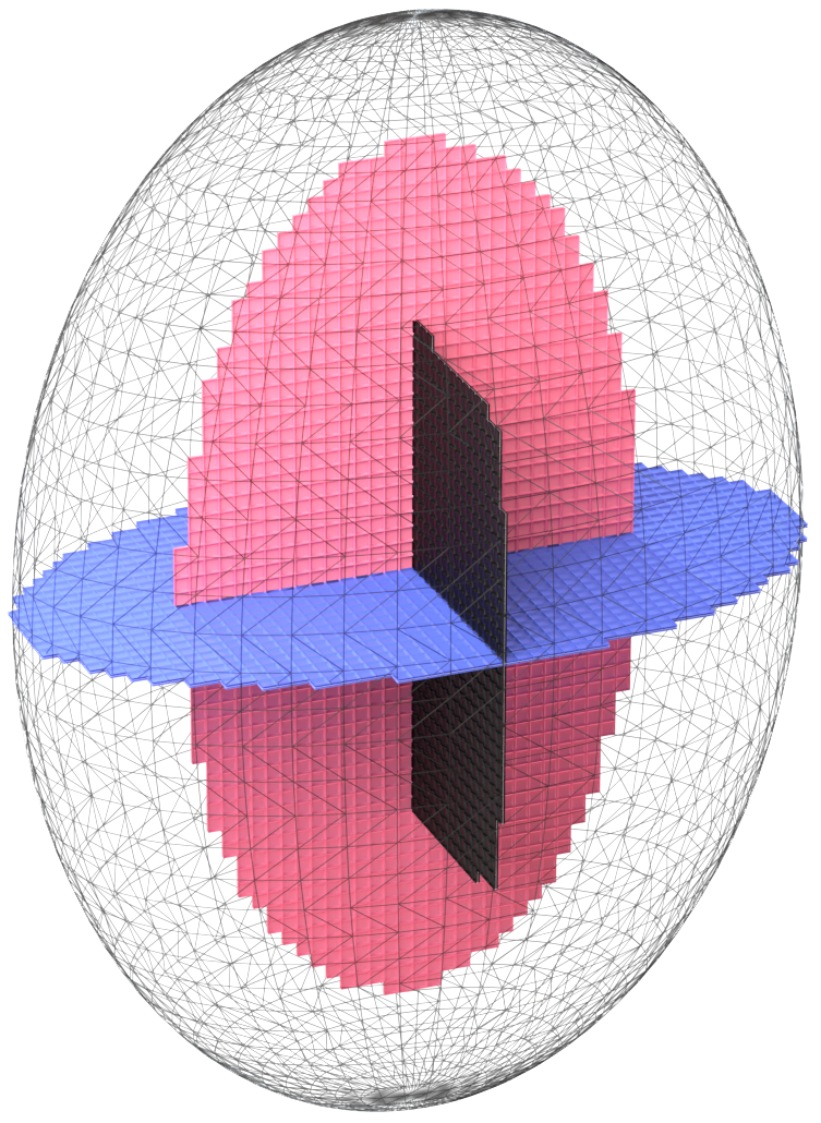
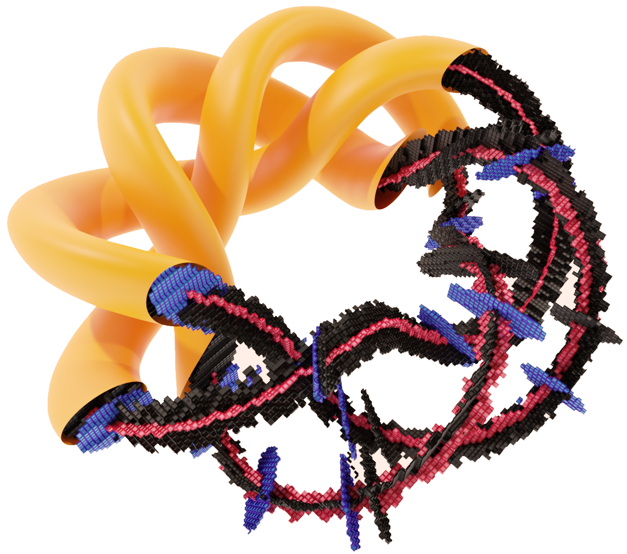
Figure 5: The pink medial, black mid-sphere, and blue circum-sphere axes of an ellipsoid on the left and an elliptically thickened $(3,7)$-torus knot on the right.

Two or more segments can be swept in parallel, so we get some mileage out of partitioning the segments connecting neighboring integer points into a few sets, which are then processed in parallel. However, no matter how we schedule the segments, the number of swaps is large. To see this note that two vertices swap along a segment iff it intersects the perpendicular bisector of the pair. Assuming we explore all segments connecting neighboring integer points in $[0,g]^{3}$, the number of such segments is $O(g^{2})$. Letting $n$ be the number of vertices in the triangulation of the surface, this amounts to a total of $O(g^{2}n^{2})$ swaps.

The matrices. Inspired by [10], we use a sparse matrix representation tailored to efficiently support the operations in the vineyard algorithm. For convenience, we use ${{\mathbb{Z}}}/2{{\mathbb{Z}}}$ coefficients so homology can be computed using boolean matrices. To reduce the boundary matrix, the algorithm swaps rows and columns, and it adds columns to each other. We thus store the matrix as a sequence of sparse columns, and we maintain permutations $\pi_{R}$ and $\pi_{C}$ for the rows and columns, respectively. With these permutations, it is easy to swap two rows or two columns, but they add an indirection when we access entries: the entry in row $i$ and column $j$ is physically stored in row $\pi_{R}(i)$ and column $\pi_{C}(j)$.

Each column is an ordered list of non-zero entries. Adding two columns means computing the xor function, and since the columns are sorted, this can be done by walking along the two lists in parallel and ignoring rows that appear in both. To decide which columns to add, the algorithm needs access to the maximum row index of the non-zero entries in a column. Because of the permutation $\pi_{R}$, this row is not necessarily the last in the list. Profiling an earlier version of our software revealed that finding this row index in a linear scan was the main bottleneck, so we decided to explicitly record this row index for each column and to update the record whenever it changes. We mention that the vineyard algorithm also adds rows to each other in a second matrix, which we support by storing the transpose of that matrix in the aforementioned format.

In spite of using sparse versions, the amount of memory needed to remember reduced matrices is significant, so we dispose of them as soon as we can while still avoiding the reduction of the boundary matrix from scratch. This is where breadth-first search in scheduling the segments shines, as its front of unfinished integer points is much smaller than for example for depth-first search.

Pruning strategies. Similar to the medial axis, the mid-sphere axis is sensitive to small fluctuations in the data, and since our algorithm is approximate, this tends to give rise to artifacts at small scales. We therefore measure scale and prune artifacts if their scale is found to be below a fixed threshold. We distinguish between two strategies: the first uses a notion of distance between the two interchanging simplices, and the second assesses their persistence.

In Euclidean pruning, we check the Euclidean distance between the two interchanging simplices. For edges and triangles, we use the Euclidean distance between their midpoints and barycenters, respectively. See Figure 6 for an illustration of the effect for different thresholds. A likely improvement would be using the geodesic distance along the surface, but we get satisfactory results with the Euclidean distance, which we use for all three types of axes.

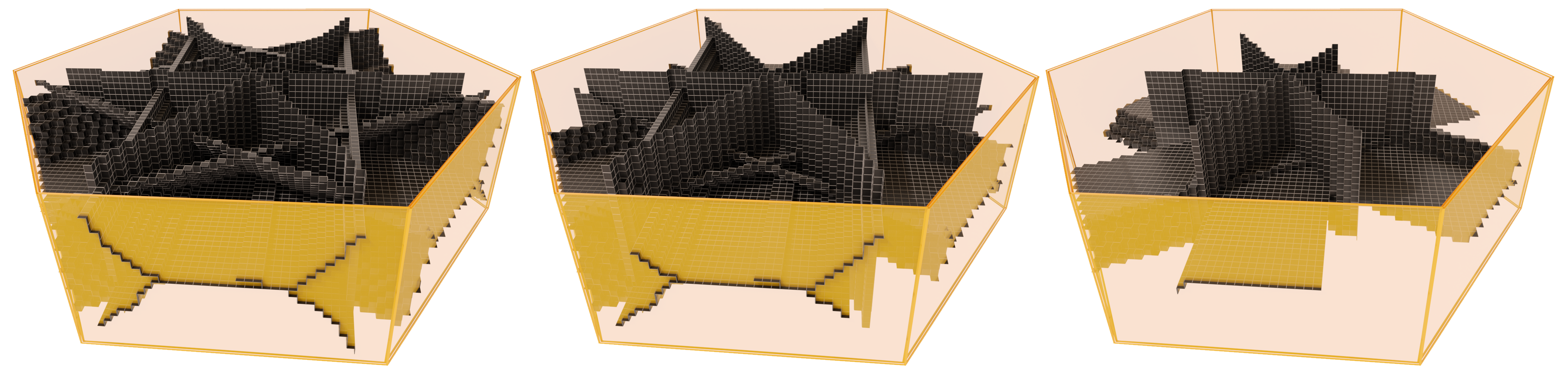
Figure 6: A hexagonal solid with its mid-sphere axis progressively modified by Euclidean pruning. The top and bottom faces of the solid are removed for improved visibility.

Alternatively, we may measure the distance combinatorially, by counting the simplices needed to connect the interchanging simplices. We use only the simplest incarnation of this idea. In face pruning, we make sure that the interchanging simplices do not have a common face, and we apply this constraint to the construction of the mid-sphere and the circum-sphere axes. Likewise, in coface pruning, we make sure that they do not have a common coface, and we apply this to the construction of the medial and the mid-sphere axes.

In persistence pruning, we consider the persistence of the two interchanging simplices; that is: their pre- and post-meditations, as defined in Section 5. We note that they have different geometric meaning: for the mid-sphere axis, the pre-meditation measures the two components inside the mid-sphere before they merge due to adding the first of the two edges, while the post-meditation measures the loop formed by adding both edges simultaneously. In our current implementation, we require that both meditations exceed a fixed threshold. We find persistence pruning indispensable for computing the mid-sphere axis, as it detects many spurious loops that form the boundaries of triangles and are filled right after being formed. More generally, we use it for all three types of axes.

Code availability. We have published the code used to compute these examples on GitHub . It can be compiled and run locally, or sampled via a live demo we have running via GitHub Pages .

7 Discussion

The main contribution of this paper is the introduction of the mid-sphere axis transform of a closed surface in ${{\mathbb{R}}}^{3}$, which is sensitive to ridge-like structures on the surface. The definition is in terms of local and global topological aspects of the family of squared distance functions on the surface from a point. We also introduce the notion of a Faustian interchange, which offers a unified framework in which the medial and the mid-sphere axis transforms are particular cases. This framework extends beyond three dimensions and leads to $d$ axis transforms for any smoothly embedded hypersurface in ${{\mathbb{R}}}^{d}$.

The presented algorithm is but a proof of the concept, and improved algorithms would be desirable. One promising idea is the extension of the Voronoi heuristic to the mid-sphere axis. Note that the Voronoi tessellation is already used to compute the standard medial axis [3], and, by analogy, the furthest-point Voronoi tessellation yields the circum-sphere axis. To extend this heuristic to the mid-sphere axis, we will have to collect and combine substructures from order-$k$ Voronoi tessellations for different orders $k$.

Another interesting direction is the analysis of effective pruning strategies that lower the sensitivity to noise in the data by defining mid-sphere axes on different scale levels. For example, can the $\lambda$-medial axis introduced by Chazal and Lieutier [8] be extended to the mid-sphere axis?

References

- [1]
- [2] E.M. Andreev. Convex polyhedra in Lobačevskiĭ spaces. Mat. Sb., New Series 81 (1970), 445–478.
- [3] D. Attali, and J-D. Boissonnat, and H. Edelsbrunner. Stability and computation of medial axes—a state-of-the-art report. Springer, Berlin Heidelberg (2009), 109–125.
- [4] E. Bittar, N. Tsingos and M. Gascuel. Automatic reconstruction of unstructured 3D data: combining a medial axis and implicit surfaces. Computer Graphics Forum 14 (1995), 457–468.
- [5] H. Blum. A transformation for extracting new descriptors of shape. In Proceedings of the Symposium on Models for the Perception of Speech and Visual Form, ed.: W.W. Dunn, MIT Press, Cambridge, Massachusetts, 1967, 362–380.
- [6] J.W. Bruce, P.J. Giblin and C.G. Gibson. Symmetry sets. Proc. Royal Soc. Edinburgh Section A: Mathematics 101 (1985), 163–186.
- [7] J. Cerf. Sur les difféomorphismes de la sphère de dimension trois (). Lecture Notes in Mathematics 53, Springer-Verlag, Berlin-New York, 1968.
- [8] F. Chazal and A. Lieutier. The -medial axis. Graph. Models 67 (2005), 304–331.
- [9] D. Cohen-Steiner, H. Edelsbrunner and J. Harer. Stability of persistence diagrams. Discrete Comput. Geom. 37 (2007), 103–120.
- [10] D. Cohen-Steiner, H. Edelsbrunner and D. Morozov. Vines and vineyards by updating persistence in linear time. In “Proc. 22nd Ann. Sympos. Comput. Geom., 2006”, 119–126.
- [11] H. Edelsbrunner and J.L. Harer. Computational Topology. An Introduction. Amer. Math. Soc., Providence, Rhode Island, 2010.
- [12] H. Federer. Curvature measures. Trans. Amer. Math. Soc. 93 (1959), 418–491.
- [13] P. Koebe. Kontaktprobleme der konformen Abbildung. Ber. Sächs. Akad. Wiss. Leipzig, Math.-Phys. Kl. 88 (1936), 141–164.
- [14] J. Milnor. Morse Theory. Princeton Univ. Press, Princeton, New Jersey, 1963.
- [15] I.R. Porteous. Geometric Differentiation. Cambridge Univ. Press, Cambridge, England, 2001.
- [16] R. Tam and W. Heidrich. Shape simplification based on the medial axis transform. In “Proc. IEEE Visualization, 2003”, 63–71.
- [17] W. Thurston. The Geometry and Topology of Three-manifolds. Electronic version, MSRI, Berkely, California, 2002.
- [18] B. Yang and J. Yao. DMAT: Deformable medial axis transform for animated mesh approximation. Computer Graphics Forum 37 (2018), 301–311.
- [19]