A New Impossibility Result for Online Bipartite Matching Problems

Abstract

Online Bipartite Matching with random user arrival is a fundamental problem in the online advertisement ecosystem. Over the last 30 years, many algorithms and impossibility results have been developed for this problem. In particular, the latest impossibility result was established by Manshadi, Oveis Gharan and Saberi [mos11] in 2011. Since then, several algorithms have been published in an effort to narrow the gap between the upper and the lower bounds on the competitive ratio.

In this paper we show that no algorithm can achieve a competitive ratio better than $1-\frac{e}{e^{e}}=0.82062\ldots$, improving upon the $0.823$ upper bound presented in [mos11]. Our construction is simple to state, accompanied by a fully analytic proof, and yields a competitive ratio bound intriguingly similar to $1-\frac{1}{e}$, the optimal competitive ratio for the fully adversarial Online Bipartite Matching problem.

Although the tightness of our upper bound remains an open question, we show that our construction is extremal in a natural class of instances.

1 Introduction

Online Bipartite Matching problems are central to the online advertising ecosystem [mos11, my11, kmt11, mehta13] and have numerous other applications, including efficient packet switching and routing [az06, ap02], crowdsourcing tasks [tsdwc16], market clearing problems [bsz06] and ride-sharing platform optimization [dssx21]. In this paper, we establish a new upper bound of $1-e^{1-e}$ on the competitive ratio for several well-studied variants of the problem. This result marks the first improvement of the upper bound for this classic problem in more than a decade.

To explain our result in context, we begin by recalling the problem. We are given a bipartite graph where one side of the bipartition consists of a known set of “ads” (or “advertisers”), while the other side consists of “users” (or “ad slots”), whose neighbor sets are initially unknown. Users arrive sequentially, and the generic user’s neighbors are revealed upon arrival. When a user arrives, the online algorithm can match, irrevocably, the user to one of its available neighbors; the algorithm’s aim is to maximize the size of the matching at the end of the sequence. The competitive ratio of an algorithm, in this case, is defined as the expected size of the matching produced by the algorithm divided by the expected size of the maximum possible matching. (We consider expectations since the algorithm can be randomized, and the input graph can be sampled from a distribution).

A strong motivation for studying this problem comes from online advertising, where edges represent ads that a user is interested in. Budget constraints limit how often each ad can be shown; without loss of generality, we assume that each ad can be matched to at most one user (ads with budgets allowing for multiple impressions can be reproduced multiple times in the graph). In this setting, a matching corresponds to a set of ads that will be shown to users, and the competitive ratio indicates how effectively the algorithm maximizes revenue.

This problem was introduced by Karp, Vazirani and Vazirani in a classic paper [kvv90]. In their setup, the graph and the ordering of the users were chosen adversarially, and they presented a simple algorithm called RANKING that achieves a competitive ratio of $1-e^{-1}$ (see [kvv90, gm08]), which was also proven to be tight [kvv90]. The assumptions of adversarial graphs and adversarial user orderings have since been relaxed to develop algorithms with better competitive ratios.

An important variant of the problem assumes that the user ordering is sampled uniformly at random, instead of being produced by an adversary [gm08]. Additionally, to move beyond adversarial graphs, researchers have explored probabilistic models of user behavior [msvv05]. See [mehta13] for a comprehensive overview.

In particular, consider the power set $2^{A}$ of the set of ads $A$, and let $P$ be a probability distribution over $2^{A}$. When a user arrives, a set $S$ of ads is sampled according to $P$, and the ads in $S$ become the user’s neighbors. In this setting, $P$ may be known or unknown, and both cases have been studied. This model of random bipartite graphs has been studied extensively and is motivated by modern machine learning-driven methods used to identify promising ads for users.

A particularly interesting special case of this last model, known as the “irregular cuckoo hashing” model, arises when a sample from $P$ is obtained by first sampling the degree of a user from a random variable $D$ taking values over the non-negative integers, and then sampling uniformly-at-random with replacement a number of ads equal to the sampled degree. This process generates a multiset of ads, but duplicate ads can be removed, leaving the remaining set as the user’s neighbors.

We can now state our result more precisely. We show that no online algorithm can achieve a competitive ratio greater than $1-e^{1-e}=0.82062\ldots$ across all the models discussed above. We establish our bound in the irregular cuckoo hashing model and so, by definition, the bound extends to all the other models and is the strongest known bound for all those variants. The previous strongest upper bound, established in 2011 by Manshadi, Oveis Gharan, and Saberi [mos11], was $0.823$. (Table 1 summarizes the state of the art). While our improvement is small, it is comparable in magnitude to many previous algorithmics advancements for this problem.

The upper bound of $0.823$ on the competitive ratio from [mos11] relies on the irregular cuckoo hashing constructions of Dietzfelbinger et al. [dgmmpr10] and was derived through numerical optimization, without yielding a closed-form expression. In contrast, our construction enables an exact analytical computation of its optimal competitive ratio. Furthermore, our construction uses simple rational probabilities, whereas the optimal probabilities in [mos11] remain unspecified and likely irrational.

Setting	Competitive Ratio
	Best Algorithm	Our UB	Previous Best UB
Irregular Cuckoo Hashing	$0.716$ [hsy22]	$1-\frac{e}{e^{e}}=0.820\!\mathinner{\ldotp\!\ldotp\!\ldotp}$	$0.823$ [mos11]
IID Users (Known Distribution)
IID Users (Unknown Distribution)	$0.696$ [my11]
Adversarial Graph, UAR Ordering
Adversarial Graph and Ordering	$1-\frac{1}{e}=0.632\!\mathinner{\ldotp\!\ldotp\!\ldotp}$ [kvv90, gm08]		$1-\frac{1}{e}=0.632\!\mathinner{\ldotp\!\ldotp\!\ldotp}$ [kvv90]

Table 1: Bounds for various Online Bipartite Matching problem variants. Each row corresponds to a different variant, listed in order from the easiest to the hardest.

The random graphs used to prove our bound are based on a simple random variable $D$ taking values over the non-negative integers:

$$\Pr\left[D=0\right]=\Pr\left[D=1\right]=0,\quad\Pr\left[D=d\right]=\frac{1}{d\cdot(d-1)},\text{ for }d\geq 2,$$

or, equivalently, $\Pr\left[D>d\right]=\nicefrac{{1}}{{d}}$ for each positive integer $d$. As discussed earlier, when a user arrives, a value $d$ is drawn from $D$, and $d$ ads are chosen uniformly at random (with replacement) as neighbors. The graph consists of $n$ ads and $n$ users. As we will clarify later, this distribution greedily ensures the “maximum possible” number of vertices of degree $d$ for $d=0,1,2,\ldots$, while maintaining a quasi-complete matching, i.e., one matching a $1-o(1)$ fraction of the users.

Intuitively, selecting user neighbors uniformly at random while keeping user degrees low impairs the performance of any online algorithm: over time, newly arriving users are likely to find all their randomly assigned neighbors already matched. However, establishing a strong upper bound also requires ensuring that the maximum matching remains large — this is the main technical challenge in our analysis.

Whether our upper bound is tight for some or all of the four problem variants mentioned above remains an open question. Notably, the bound involves the Euler’s number, in a manner analogous to the optimal competitive ratio of $1-\frac{1}{e}$ of the fully-adversarial Online Bipartite Matching problem. While we cannot determine whether our upper bound can be improved, we show that it possesses a certain extremal property and that it is the strongest bound possible for a natural class of instances.

Paper Organization. Section 2 gives an overview of our main construction, of its relation to previous upper bounds, and of the techniques we used to study it. Section 3 reviews related work. Section 4 introduces key tools, techniques, and notation. In Section 6, we present our construction and prove the main result: the $1-{e}^{1-e}$ upper bound on the competitive ratio of Online Bipartite Matching Problems. Section 7 establishes the extremality of our construction, showing that it greedily maximizes the number of low-degree users while ensuring a quasi-complete matching. Section 8 extends our construction to arbitrary user-to-ad ratios, demonstrating that equibipartite graphs yield the strongest bound. We conclude with open questions in Section 9.

All the proofs missing from the main body of this paper can be found in its Appendix.

2 Overview

Our irregular cuckoo hashing instance contains $n$ users and $n$ ads, and assigns probability $\frac{1}{d\cdot(d-1)}$ to each user-degree $d\geq 2$ — in other words, it posits that the probability that a user has degree strictly larger than the generic positive integer $d$ is exactly $\nicefrac{{1}}{{d}}$. We obtained this distribution by greedily maximizing the number of users of degree $d=0,1,2,3,\ldots$ while guaranteeing that the random graph admits a quasi-complete matching from the user side — a matching that pairs all users except for at most $o(n)$ of them. Observe that, in a cuckoo hashing instance, the smaller the user-degrees the less likely it is for an online algorithm to match users. The goal of our distribution is to minimize the number of online matches while guaranteeing that the graph admits a quasi-complete matching — in other words, the distribution aims to minimize the numerator of the competitive ratio while making its denominator as large as possible. (We remark that most previous upper bounds were also based on graphs admitting quasi-complete matchings; see, e.g., [bk10, mos11, gm08, kvv90].)

Our Main Construction. It is easy to see that, in order for a cuckoo hashing instance containing $n$ ads, and no more than $n$ users, to be quasi-complete from the user side, the instance must contain at most $o(n)$ users of degree $0$ and $o(n)$ users of degree $1$. Furthermore, classical results can be used to prove that, if one aims to be quasi-complete from the user side, and all users have degree $2$, then the maximum number of users is $c_{2}\cdot n\pm o(n)$, for $c_{2}=\frac{1}{2}$. Now, suppose that we must have $c_{2}\cdot n\pm o(n)$ users of degree $2$. What is the largest number of users of degree $3$ that we can add while still guaranteeing that there exists a matching covering a $1-o(1)$ fraction of the users? We prove that the answer is “$c_{3}\cdot n\pm o(n)$, for $c_{3}=\frac{1}{6}$”. Next, if we are bound to have $c_{2}\cdot n\pm o(n)$ users of degree $2$ and $c_{3}\cdot n\pm o(n)$ users of degree $3$, what is the maximum $c_{4}$ such that we can add $c_{4}\cdot n\pm o(n)$ users of degree $4$ and match a $1-o(1)$ fraction of users? And so on and so forth.

In general, we set $c_{d}=\frac{1}{d\cdot(d-1)}$ for each degree $d\geq 2$, and $c_{0}=c_{1}=0$. These fractions result in a total of $n$ users, to be matched to the $n$ ads. To establish that these $c_{d}$’s give rise to a graph admitting a quasi-complete matching we couple the irregular cuckoo hashing graph with a random graph in the configuration model having the same degree distribution on the user side, and the same Poissonian degree distribution on the ads side; then, by means of the Karp-Sipser algorithm [ks81] (which we analyze with a variant of the techniques presented in [bg15] by Balister and Gerke), we establish that this configuration model graph admits a quasi-complete matching; using the coupling, we derive the existence of a quasi-complete matching in the irregular cuckoo hashing graph, as well. Finally, we upper bound the fraction of ads matched by any online algorithm with $1-\frac{e}{e^{e}}=0.82062\ldots$, thus proving our new upper bound on the competitive ratio of several Online Bipartite Matching problems.

As an extra step, aimed at establishing the extremality of our construction, we show that if one increases any of the $c_{d}$’s by any constant $\epsilon>0$, then a constant fraction of the vertices of degree at most $d$ become unmatchable. (In particular, if the extra $\epsilon$ fraction assigned to degree $d$ is taken from vertices of higher degree, then the quasi-complete matching disappears).

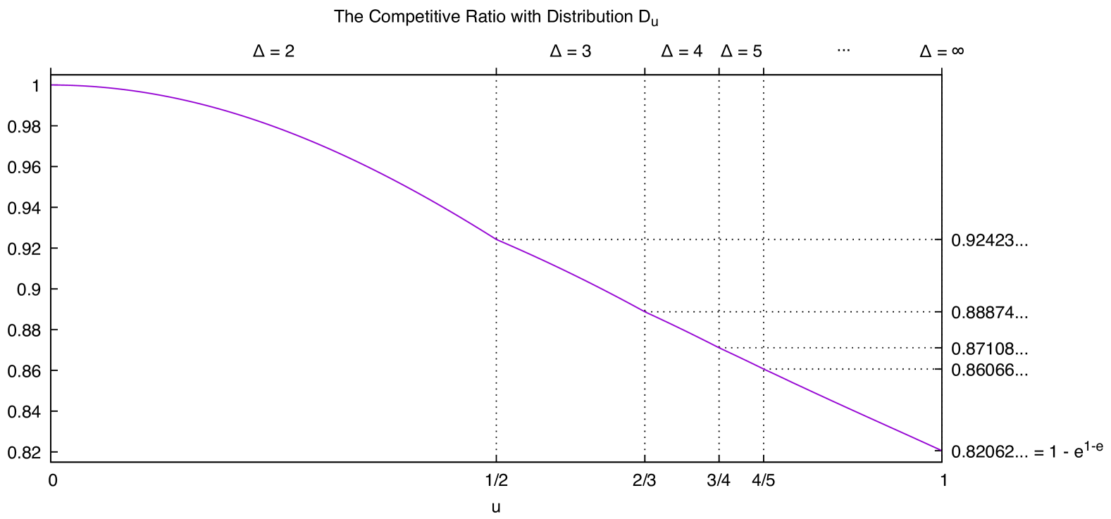
Figure 1: The Competitive Ratios induced by the $D_{u}$ instances, obtained numerically for $u>0$. The plot shows how $u=1$ (which corresponds to the case of unbounded user-degree) gives the strongest upper bound. In Theorem 8, we analytically establish the optimality of $u=1$.

A Class of Constructions. Our construction has users of unbounded degree, and contains the same number of users and ads. To get a more thorough understanding of the construction, and of the problem, we study a class of constructions that generalizes our main one; the instances in this class have $n$ ads, and $u\cdot n$ users. Just like our main construction, we populate the generic instance in the class by greedily adding users with the smallest possible degree, under the constraint that the instance admits a quasi-complete matching. For a given $u\in(0,1)$, the generalized instance $D_{u}$ has a maximum user degree of $\left\lceil\frac{1}{1-u}\right\rceil$. We prove that, for all $u\in(0,1)$, these instances give a weaker upper bound on the competitive ratio than the case $u=1$, that is, the case with $n$ users and $n$ ads (see Figure 1 and Theorem 8).

Previous Constructions. We point out that studying instances of varying user degrees is necessary to improve over the state of the art. In particular, if an irregular cuckoo hashing instance has $n$ users and $n$ ads, and all the users have degree $1$, any greedy online algorithm will necessarily return a maximum matching (which matches a fraction of $1-\frac{1}{e}=0.63212\ldots$ users). Thus, the best upper bound provable with this instance is $1$. If, instead, each user has degree $2$, a greedy online algorithm will return a matching with, roughly, $\tanh(1)\cdot n=0.76159\ldots\cdot n$ edges. The maximum matching has size approximately equal to $\left(1+\frac{1}{2}W\left(-2e^{-2}\right)+\frac{1}{4}W\left(-2e^{-2}\right)^{2}\right)\cdot n=0.83809\ldots\cdot n$ (see, e.g., [khk11]; here, $W$ is the Lambert W function), so that the best upper bound provable with this instance is $0.90871\ldots$. Finally, if each user has degree $3$ or more, one can show that the number of users matched by any greedy online algorithm is at least $0.82304\ldots\cdot n$. It follows that having a uniform user degree in equibipartite graphs makes it impossible to improve upon—or even match—the $0.823$ upper bound of Manshadi et al. [mos11].

Indeed, Manshadi et al. [mos11] derived their upper bound by employing a mixture of users with varying degrees. In their construction, the user degree distribution is supported on $\{2,3,n\}$. Manshadi et al.’s analysis leverages on an irregular cuckoo hashing construction of Dietzfelbinger et al. [dgmmpr10], whose parameters were obtained numerically; as a result, the optimal fractions of vertices of degrees $2$ and $3$ in the bipartite matching result of [mos11] are not given explicitly (and might very well be irrational numbers). Our extremal construction, instead, allows us to compute the competitive ratio analytically and exactly, and is made up of simple, rational, probabilities.

3 Related Work

Online Bipartite Matching problems have a long history. We mention here the results that are most relevant to our paper; see the book of Mehta [mehta13], or the recent survey of Huang, Tang and Wajc [htw24], for a more comprehensive introduction to these problems.

As we mentioned before, if the graph and the ordering are adversarial, then a competitive ratio of $1-\frac{1}{e}$ can be achieved via the RANKING algorithm of Karp, Vazirani and Vazirani [kvv90] (see, Goel and Mehta [gm08], or Birnbaum and Mathieu [bm08], for proofs; simpler analyses were given in, e.g., Devanur, Jain and Kleinberg [djk13] and Eden et al. [effs21]): this algorithm begins by sampling a uniform-at-random ordering of the ads; whenever a user arrives, if at least one ad is available for that user, the user is matched to the first available ad in the ordering. As shown in [kvv90], the competitive ratio of the RANKING algorithm, $1-\frac{1}{e}$, is optimal in the fully-adversarial case.

Determining the optimal competitive ratio if the set of users is permuted uniformly-at-random is, possibly, the most important open problem in this area. The best known upper bound on the competitive ratio of this problem was proved by Manshadi, Oveis Gharan and Saberi [mos11, mos12] and has value $0.823$ — this upper bound holds regardless of whether the bipartite graph is generated adversarially or randomly. The RANKING algorithm is still the best known algorithm for this problem on adversarial graphs; Mahdian and Yan[my11] show that it achieves a competitive ratio of at least $0.696$, and Karande, Mehta and Tripathi [kmt11] show that its competitive ratio is not larger than $0.727$.

The case of randomized bipartite graphs has also been studied extensively; in this setting the adversary produces a distribution over subsets of ads, and each user samples independently a set of ads from that distribution. In the “known distribution” case, this distribution is assumed to be known to the algorithm; the “unknown distribution” variant has also been studied extensively. As mentioned in the previous paragraph, Mahdian and Yan [my11] gave an algorithm for randomly-permuted adversarial graphs with a competitive ratio of $0.696$; this algorithm applies to both the known, and the unknown, distribution cases. Several improvements on the competitive ratio for the known distribution case have been proved in the last fifteen years. In 2011, Manshadi et al. [mos11], proposed an algorithm with a competitive ratio of $0.702$. In 2014, Jaillet and Lu[jl14] had an algorithm achieving a competitive ratio of $0.706$. Then, in 2021, Huang and Shu [hs21] gave an algorithm with a competitive ratio of $0.711$; finally, in 2022, Huang, Shu and Yan[hsy22] achieved a competitive ratio of $0.716$.

The best impossibility result so far — which holds in the cases of adversarial graph with UAR ordering, of random graphs with unknown distribution, and known distribution, as well as in the irregular cuckoo hashing case — is the aforementioned upper bound of $0.823$ published by Manshadi et al. in 2011 [mos11]. Our result improves the bounds in each of these four cases from $0.823$ to $1-\frac{e}{e^{e}}=0.82062\ldots$. We remark that our numerical improvement, of value roughly $0.002$, is of the same order of all the algorithmic improvements mentioned in the previous paragraph.

Several special cases of online bipartite matching problems have been studied in the last few years. In particular, the “integral arrival rates” special case of the “known distribution” setting requires that each set in the support of the distribution has an integral expected number of occurrences. For this case, the best known algorithm — due to Brubach et al. [bssx16] — achieves a competitive ratio of $0.7299$; the best known upper bound for the integral arrival rates case has value $1-e^{-2}=0.864\ldots$, and is due to Manshadi et al. [mos12].

We conclude this section by noting that the interest in online bipartite matching is further evidenced by the attention given in recent years to several related problems. These include some of its weighted [hsy22, knr22, fhtz22], and fairness-aware [mx24], variants; in particular, Huang et al. [hsy22] show an upper bound of $0.703$ for the (known distribution) edge-weighted online bipartite matching problem, whereas Ma and Xu [mx24] show an upper bound of $\sqrt{3}-1=0.732\ldots$ for a variant whose goal is to maximize the minimum matching rate across different groups of users. Other related problems include fractional variants and their rounding schemes [tz24, nsw25, ss18, bnw23, bsvw24], variants with different probing models [bm25, bmr21, bmr22], those with time-dependent user distributions [bdpsw25, tww22, ppsw21, bdm22], with users arriving in batches [fns21, fns24, jm22] or with different arrival models [bst19, gkmsw19, efgt22], variants that leverage machine-learned advice [cglb24, agkk23, jm22], as well as generalized selection tasks [hjpsz24, ghhnyz21].

4 Preliminaries

We present here the objects, the tools and the notation that we will use in this paper.

Notation. Given a predicate $P$, the Iverson bracket $[P]$ has value $1$ if $P$ is true, and value $0$ otherwise. With a slight abuse of notation, for a positive integer $n$, we use $[n]$ to denote the set $[n]=\{1,\dots,n\}$. The support of a multiset $S$ is the set of elements whose multiplicity in $S$ is at least $1$. For an integer $k\geq 1$, we let $H_{k}=\sum_{i=1}^{k}\frac{1}{i}$ be the $k$-th harmonic number. Finally, we let $\Phi(z,s,\alpha)=\sum_{k=0}^{\infty}\frac{z^{k}}{(k+\alpha)^{s}}$ be the Lerch transcendent, a series that generalizes the Riemann $\zeta$ function, and which converges if $\alpha>0$, $|z|<1$ and $s\in\mathbf{R}$.

Bipartite (Multi)Graphs and Matchings. An undirected bipartite (multi)graph $G(V,\hat{V},E)$ is defined by two disjoint sets of vertices $V$ and $\hat{V}$, and by a (multi)set of edges $E$ having a support set which is a subset of $\{\{v,\hat{v}\}\mid v\in V\wedge\hat{v}\in\hat{V}\}$. If $E$ coincides with its support set, then $G(V,\hat{V},E)$ has no parallel edges, and we say that $G(V,\hat{V},E)$ is a simple graph. We will typically use $V=\{v_{1},v_{2},\dots\}$ to denote the set of users, and $\hat{V}=\{\hat{v}_{1},\hat{v}_{2},\dots\}$ to denote the set of ads. We will also use $n_{i}$ (resp., $\hat{n}_{i}$) to denote the number of vertices of degree $i\geq 0$ in $V$ (resp., $\hat{V}$).

A matching $M$ in the (multi)graph $G(V,\hat{V},E)$ is a subset $M\subseteq E$ containing pairwise disjoint edges. We say that $G(V,\hat{V},E)$ admits a complete matching if there exists a matching $M\subseteq E$ of $G(V,\hat{V},E)$ such that $|M|=\min(|V|,|\hat{V}|)$, and that it admits a perfect matching if there exists a matching $M\subseteq E$ such that $|M|=|V|=|\hat{V}|$.

Given a bipartite multigraph $G(V,\hat{V},E)$, if $E^{\prime}$ is the support set of $E$, we have that $G(V,\hat{V},E^{\prime})$ is a bipartite simple graph. Observe that each matching of $G(V,\hat{V},E^{\prime})$ is also a matching of $G(V,\hat{V},E)$; moreover, given an arbitrary matching $M$ of $G(V,\hat{V},E)$, we can transform $M$ into a matching of $G(V,\hat{V},E^{\prime})$ by substituting, for each $e\in M$, the edge $e$ with its unique parallel edge $e^{\prime}\in E^{\prime}$.

We say that an infinite sequence of bipartite (multi)graphs $G(V_{1},\hat{V}_{1},E_{1}),G(V_{2},\hat{V}_{2},E_{2}),\ldots$ of increasing side sizes ($\min(|V_{1}|,|\hat{V}_{1}|)<\min(|V_{2}|,|\hat{V}_{2}|)<\cdots$), and with maximum matchings $M_{1}\subseteq E_{1},M_{2}\subseteq E_{2},\ldots$, admits a quasi-complete matching if $|M_{i}|\geq(1-o(1))\cdot\min(|V_{i}|,|\hat{V}_{i}|)$ — that is, if for each $\epsilon>0$ there exists $i^{\star}$ such that, for each $i\geq i^{\star}$, $|M_{i}|\geq(1-\epsilon)\cdot\min(|V_{i}|,|\hat{V}_{i}|)$.

The Karp-Sipser Algorithm. The Karp-Sipser algorithm [ks81] is a greedy algorithm for computing a matching of a graph. A run of this algorithm is divided in two phases; for our purposes, only the first phase will be necessary. During the first phase, the algorithm looks for any vertex of degree $1$; as long as such a vertex exists, the algorithm adds its incident edge $e$ to a set $S$, removes the two endpoints of $e$ from the graph, and iterates. If no such vertex exists, the first phase ends. It is easy to prove that, at any point during the execution of the first phase, the set $S$ can be extended to a maximum matching of the original graph. In fact, it is also easy to prove that if the original graph $G(V,\hat{V},E)$ is bipartite and, at any point during the execution of the first phase, $V_{0}\subseteq V$ (resp. $\hat{V}_{0}\subseteq\hat{V}$) is the subset of $V$ (resp. $\hat{V}$) containing vertices that have current degree $0$ and which are still unmatched, then the maximum matching cannot be larger than $\min\left(|V|-|V_{0}|,|\hat{V}|-|\hat{V}_{0}|\right)$.

The Karp-Sipser algorithm was introduced to bound the size of the maximum matching in sparse $G(n,p)$ random graphs; since its introduction, the algorithm has been used to bound the size of the maximum matching of many other random graph models.

The Irregular Cuckoo Hashing Model. For simplicity of exposition, the random graph models that we will consider in this paper might produce non-simple graphs, that is, multigraphs with parallel edges; these can be easily transformed into simple graphs through the removal of parallel edges. One of the two random graph models that we will consider is the irregular cuckoo hashing model, which is defined as follows: [Irregular Cuckoo Hashing Model] Let $n,m$ be two positive integers, and $P$ be a probability distribution over the non-negative integers. The Irregular Cuckoo Hashing random multigraph $\operatorname*{ICH}(n,m,P)$ is defined as follows. This bipartite graph has user set $V$ and ads set $\hat{V}$, with $n=|V|$ and $m=|\hat{V}|$. Each user $v_{i}\in V$ samples independently an integer $d_{i}$ from $P$ and, for each $j=1,2,\ldots,d_{i}$, samples independently an ad $\hat{v}_{i,j}$ uniformly at random from $\hat{V}$. The multiset of neighbors of $v_{i}$ is $\{\hat{v}_{i,1},\ldots,\hat{v}_{i,d_{i}}\}$. (Note that $\operatorname*{ICH}(n,m,P)$ might not be simple).

The Configuration Model. In order to analyze the irregular cuckoo hashing graph of our construction, we will couple it with a random graph in the configuration model. [Configuration Model] Consider two sequences of non-negative integers $\mathbf{d}=(d_{1},\dots,d_{n})$ and $\mathbf{\hat{d}}=(\hat{d}_{1},\dots,\hat{d}_{m})$ such that $\sum_{i=1}^{n}d_{i}=\sum_{i=1}^{m}\hat{d}_{i}$. To sample a bipartite graph $G=(V,\hat{V},E)$ from the configuration model $\operatorname*{CM}(\mathbf{d},\mathbf{\hat{d}})$, for each $i\in[n]$ (resp. $j\in[m]$), assign to vertex $v_{i}$ (resp. $\hat{v}_{j}$) $d_{i}$ (resp. $\hat{d}_{j}$) configuration points, and then sample a uniform at random perfect bipartite matching between the configuration points. (Note that $\operatorname*{CM}(\mathbf{d},\mathbf{\hat{d}})$ might not be simple). To compute the size of the maximum matching in our configuration model distribution, we will study the behavior of the first phase of the Karp-Sipser algorithm using the techniques presented, e.g., by Balister and Gerke in [bg15] (see also [afp98, bf11]). In particular, we will show that our distribution admits a quasi-complete matching through the following modification of a result in [bg15]: Let $\rho\in(0,1]$ be any constant. Let $f(x)=\sum_{i=0}^{\infty}z_{i}\cdot x^{i}$, and $\hat{f}(x)=\sum_{i=0}^{\infty}\hat{z}_{i}\cdot x^{i}$, where $(z_{i})_{i=0}^{\infty},(\hat{z}_{i})_{i=0}^{\infty}$ are non-negative sequences such that $f^{\prime}(1)=\hat{f}^{\prime}(1)=\mu<\infty$ and $f^{\prime}(2),\hat{f}^{\prime}(2)<\infty$. Consider any configuration model $\operatorname*{CM}(\mathbf{d},\mathbf{\hat{d}})$, with $|\mathbf{d}|=f(1)n\pm o(n)$, $|\mathbf{\hat{d}}|=\hat{f}(1)n\pm o(n)$, and such that (i) $n_{i}=(z_{i}\pm o(n^{-\rho}))n$ for $i\geq 0$, (ii) $\hat{n}_{i}=(\hat{z}_{i}\pm o(n^{-\rho}))n$ for $i\geq 0$, (iii) $|E|=(\mu\pm o(n^{-\rho}))n$, and (iv) for $M=M(n)=\Theta(\log n)$, $\sum_{i=M}^{\infty}i^{2}\cdot z_{i}=o(n^{-\rho})$ and $\sum_{i=M}^{\infty}i^{2}\cdot\hat{z}_{i}=o(n^{-\rho})$, where $n_{i}$ (resp. $\hat{n}_{i}$) is the number of vertices of degree $i$ in $\mathbf{d}$ (resp. $\mathbf{\hat{d}}$).

Let $w_{2},\hat{w}_{1}\in[0,1]$ be the smallest solutions to the simultaneous equations $w_{2}=1-\frac{f^{\prime}(1-\hat{w}_{1})}{\mu}$, $\hat{w}_{1}=\frac{\hat{f}^{\prime}(w_{2})}{\mu}$. Then, with probability $1-o(1)$, the first phase of Karp-Sipser, on the graph $G(V,\hat{V},E)\sim\operatorname*{CM}(\mathbf{d},\mathbf{\hat{d}})$, returns a matching of size at least

$$(f(1)-f(1-\hat{w}_{1})-f^{\prime}(1-\hat{w}_{1})\hat{w}_{1}-o(1))n.$$

Moreover, with probability $1-o(1)$, after the first phase of Karp-Sipser, at least $(\hat{f}(w_{2})-f(1)+f(1-\hat{w}_{1})+f^{\prime}(1-\hat{w}_{1})\hat{w}_{1}-o(1))n$ vertices in $\hat{V}$ will be isolated (i.e., of degree 0 and unmatched). Equivalently, with probability $1-o(1)$, the maximum matching cannot be larger than,

$$(\hat{f}(1)-\hat{f}(w_{2})+f(1)-f(1-\hat{w}_{1})-f^{\prime}(1-\hat{w}_{1})\hat{w}_{1}+o(1))n.$$

5 Adaptation of the Analysis of Balister and Gerke to Unbounded Degree Distributions

In this section we adapt the analysis of [bg15] for the first phase of the Karp-Sipser algorithm, so to allow unbounded maximum degree. Note that the original analysis can be used by first limiting the maximum degree to a constant and by truncating the generating functions $f$ and $\hat{f}$ defined below; in our case, however, the original distribution makes it possible to apply several algebraic shortcuts that become infeasible once the distribution is transformed into one having finite support. Therefore, we found it simpler to modify Balister and Gerke’s analysis so to accommodate distributions with unbounded support.

The analysis of [bg15] considers a slight variation of the first phase of Karp-Sipser. The algorithm proceeds in rounds; in particular, all degree-1 vertices of round $t$ are analyzed before moving to round $t+1$. The degree-1 vertices of round $t+1$ are those that were generated in round $t$. This slight modification still has the property that, at any point, the current matching can be extended to a maximum one.

Define the generating functions $f(x)=\sum_{i=0}^{\infty}z_{i}\cdot x^{i}$ and $\hat{f}(x)=\sum_{i=0}^{\infty}\hat{z}_{i}\cdot x^{i}$, where $(z_{i})_{i=0}^{\infty}$ and $(\hat{z}_{i})_{i=0}^{\infty}$ are two non-negative sequences, and we adopt the standard convention $0^{0}=1$. We assume that $f^{\prime}(1)=\hat{f}^{\prime}(1)=\mu<\infty$, and $f^{\prime}(2)=\sum_{i=1}^{\infty}z_{i}\cdot i\cdot 2^{i-1}<\infty$, $\hat{f}^{\prime}(2)=\sum_{i=1}^{\infty}\hat{z}_{i}\cdot i\cdot 2^{i-1}<\infty$. Note that this also implies $f^{\prime\prime}(1)<\infty$, $\hat{f}^{\prime\prime}(1)<\infty$, $\sum_{i=1}^{\infty}z_{i}\cdot i\cdot 2^{i}<\infty$, and $\sum_{i=1}^{\infty}\hat{z}_{i}\cdot i\cdot 2^{i}<\infty$. Consider any configuration model $\operatorname*{CM}(\mathbf{d},\mathbf{\hat{d}})$, with $|\mathbf{d}|=f(1)n\pm o(n)$, $|\mathbf{\hat{d}}|=\hat{f}(1)n\pm o(n)$, and such that:

1. $n_{i}=(z_{i}\pm o(n^{-\rho}))n$ for $i\geq 0$

2. $\hat{n}_{i}=(\hat{z}_{i}\pm o(n^{-\rho}))n$ for $i\geq 0$

3. $|E|=(\mu\pm o(n^{-\rho}))n$

4. for $M=M(n)=\Theta(\log n)$, $\sum_{i=M}^{\infty}i^{2}\cdot z_{i}=o(n^{-\rho})$ and $\sum_{i=M}^{\infty}i^{2}\cdot\hat{z}_{i}=o(n^{-\rho})$

where $\rho\in(0,1]$ is a constant, and $n_{i}$ (resp. $\hat{n}_{i}$) is the number of vertices of degree $i$ in $\mathbf{d}$ (resp. $\mathbf{\hat{d}}$).

As a first step, similarly to [bg15], we limit the maximum degree to $M$. Note that, however, we will not modify the definitions of $f$ and $\hat{f}$. Specifically, we remove all configuration points of the vertices having degree larger than $M$. Therefore, on one side of the bipartite graph, we remove a number of configuration points equal to

$$\sum_{i=M+1}^{\infty}in_{i} =|E|-\sum_{i=0}^{M}in_{i}=n\sum_{i=0}^{\infty}iz_{i}-n\sum_{i=0}^{M}iz_{i}\pm o(n^{1-\rho}M^{2})\leq o(n^{1-\rho}M^{2})\leq o(n^{1-\rho^{\prime}}),$$

for some new constant $0<\rho^{\prime}<\rho$. After removing $o(n^{1-\rho^{\prime}})$ configuration points from the other side of the bipartite graph, and further removing $o(n^{1-\rho^{\prime}})$ configuration points to ensure that the sum of the degrees remains the same on the two sides; we end up with a configuration model having a maximum degree of $M=O(\log n)$, but since we only removed $o(n^{1-\rho^{\prime}})$ edges, properties 1-4 above still hold (albeit with a different constant $\rho$) and the size of the maximum matching is the same up to an $o(n)$ error. For simplicity, we will keep on using $\rho$ in place of $\rho^{\prime}$.

Let us sample a graph $G(V,\hat{V},E)$ from such configuration model. A vertex $v\in V\cup\hat{V}$ is called $t$-good if its $t$-neighborhood (i.e., $v$ and all the vertices at distance at most $t$ from $v$) is a tree, otherwise it is called $t$-bad. (Note that a vertex with parallel edges is also considered $t$-bad.) The following result only relies on $M^{t}=c^{o(\log n)}$ for some constant $c$.

[[bg15], Lemma 3.4] If $t=o\left(\frac{\log n}{\log\log n}\right)$, with probability $1-o(1)$, the number of $t$-bad vertices is $o(n)$.

Fix a $t$-good vertex $v$. Consider the tree rooted at $v$. Starting from $v$, we number the levels of the tree from 1 to $t+1$. Consider the vertices different from the root, we classify them as follows. All vertices at level $t+1$ are $v$-normal. Consider a vertex $u$ at level $\ell$. If all its children at level $\ell+1$ are $v$-popular, then $u$ is $v$-lonely (this considers also the case where there are no children at level $\ell+1$). If at least one of its children is $v$-lonely, then $u$ is $v$-popular. Otherwise, $u$ is $v$-normal. The root $v$ is lonely wrt $t$ if all its children are $v$-popular (or it has no children), it is popular wrt $t$ if at least two of its children are $v$-lonely, otherwise it is normal wrt $t$. The following result only uses the classification of the vertices.

[[bg15], Lemma 3.5] Suppose $v$ is $t$-good, for $t\geq 1$. If $v$ is popular wrt $t$, it will be matched within the first $\lfloor t/2\rfloor$ rounds of the first phase of the Karp-Sipser Algorithm. If $v$ is lonely wrt $t$, in the first $\lfloor t/2\rfloor$ rounds, it will either become isolated (i.e., of degree $0$ and unmatched) or it will be matched to a vertex $u$ which is popular wrt $t-1$.

Define inductively, $\hat{w}_{1}^{(1)}=w_{2}^{(1)}=0$, and $\hat{w}_{1}^{(t)}=\frac{\hat{f}^{\prime}(w_{2}^{(t-1)})}{\mu}$, $w_{2}^{(t)}=1-\frac{f^{\prime}(1-\hat{w}_{1}^{(t-1)})}{\mu}$ for $t>1$. Let $(\hat{w}_{1},w_{2})$ be the smallest non-negative solution of the simultaneous equations $\hat{w}_{1}=\frac{\hat{f}^{\prime}(w_{2})}{\mu}$, $w_{2}=1-\frac{f^{\prime}(1-\hat{w}_{1})}{\mu}$. As $t$ goes to infinity, $(\hat{w}_{1}^{(t)},w_{2}^{(t)})$ converges to $(\hat{w}_{1},w_{2})$, since it is a bounded increasing sequence. Indeed, the next Lemma shows that $\hat{w}_{1}^{(i)}$ and ${w}_{2}^{(i)}$ are probabilities. We need to adapt the original proof of [bg15] for this Lemma because we use the original, non-truncated, generating functions $f$ and $\hat{f}$. Specifically, we will use that $\sum_{i=0}^{M}z_{i}\cdot x^{i}=f(x)\pm o(n^{-\rho})$ for $x\in[0,1]$, and similarly for $f^{\prime}$, $f^{\prime\prime}$, $\hat{f}$, $\hat{f}^{\prime}$, and $\hat{f}^{\prime\prime}$.

[Adaptation of [bg15], Theorem 3.6] Let $t=o\left(\frac{\log n}{\log\log n}\right)$, and let $v$ be a $t$-good vertex. For all $i\in\{1,\dots,t\}$, the following holds:

1. The probability that a vertex $u\in\hat{V}$ at distance $t+1-i$ from $v$ is $v$-lonely wrt $t$, conditioned on its existence and the tree rooted at $v$ except for the branch rooted at $u$, is $\hat{w}_{1}^{(i)}\pm O(M^{t+i}\cdot n^{-\rho})$

2. The probability that a vertex $u\in V$ at distance $t+1-i$ from $v$ is $v$-popular wrt $t$, conditioned on its existence and the tree rooted at $v$ except for the branch rooted at $u$, is $w_{2}^{(i)}\pm O(M^{t+i}\cdot n^{-\rho})$

The results are true even conditioning on at most $O(M^{t})$ edges outside of the $t$-neighborhood of $v$.

Proof.

Both results are true for $i=1$, as all vertices at level $t+1$ are $v$-normal. Let $i>1$. We start by proving the first point. Fix a vertex $u\in\hat{V}$ at distance $t+1-i$, the probability that it is $v$-lonely is:

$$\sum_{k=0}^{M-1}\Pr[u\text{ has children }u_{1},\dots,u_{k}]\prod_{j=1}^{k}\Pr[u_{j}\text{ is $v$-popular}\mid u_{1},\dots,u_{j-1}\text{ are $v$-popular}].$$

Considering the conditioning of at most $O(M^{t})$ edges, the probability that $u$ has degree $k+1$ is:

$$\frac{(k+1)(\hat{z}_{k+1}\pm o(n^{-\rho}))n-O(M^{t})}{(\mu\pm o(n^{-\rho}))n-O(M^{t})} =\frac{(k+1)\hat{z}_{k+1}}{\mu}\pm O\left(\frac{M^{t}}{n}\right)\pm o\left(\frac{k}{n^{\rho}}\right)=\frac{(k+1)\hat{z}_{k+1}}{\mu}\pm O\left(\frac{M^{t}}{n^{\rho}}\right).$$

Now, the probability of $u_{j}$ being $v$-popular is by inductive hypothesis $w_{2}^{(i-1)}\pm O(M^{t+i-1}n^{-\rho})$. Note also that $\left(w_{2}^{(i-1)}\pm O(M^{t+i-1}n^{-\rho})\right)^{k}=(w_{2}^{(i-1)})^{k}\pm k\cdot O(M^{t+i-1}n^{-\rho})$, since we can discard lower order terms. Putting things together, the previous probability becomes:

$$\sum_{k=0}^{M-1}\frac{(k+1)\hat{z}_{k+1}}{\mu}\cdot\left(w_{2}^{(i-1)}\pm O\left(\frac{M^{t+i-1}}{n^{\rho}}\right)\right)^{k}\pm O\left(\frac{M^{t+1}}{n^{\rho}}\right)$$

$$=\sum_{k=0}^{M-1}\frac{(k+1)\hat{z}_{k+1}}{\mu}\cdot\left(w_{2}^{(i-1)}\right)^{k}\pm O\left(\frac{M^{t+i-1}}{n^{\rho}}\right)\sum_{k=0}^{M-1}\frac{k(k+1)\hat{z}_{k+1}}{\mu}\pm O\left(\frac{M^{t+1}}{n^{\rho}}\right)$$

$$=\frac{1}{\mu}\left(\sum_{k=1}^{\infty}k\hat{z}_{k}\left(w_{2}^{(i-1)}\right)^{k-1}-\sum_{k=M+1}^{\infty}k\hat{z}_{k}\left(w_{2}^{(i-1)}\right)^{k-1}\right)\pm O\left(\frac{M^{t+1}}{n^{\rho}}\right)$$

$$\quad\pm O\left(\frac{M^{t+i-1}}{n^{\rho}}\right)\frac{1}{\mu}\left(\sum_{k=2}^{\infty}(k-1)k\hat{z}_{k}-\sum_{k=M+1}^{\infty}(k-1)k\hat{z}_{k}\right)$$

$$=\frac{1}{\mu}\left(\hat{f}^{\prime}(w_{2}^{(i-1)})-o(n^{-\rho})\right)\pm O\left(\frac{M^{t+i-1}}{n^{\rho}}\right)\frac{1}{\mu}\left(\hat{f}^{\prime\prime}(1)-o(n^{-\rho})\right)\pm O\left(\frac{M^{t+1}}{n^{\rho}}\right)$$

$$=\frac{\hat{f}^{\prime}(w_{2}^{(i-1)})}{\mu}\pm O\left(\frac{M^{t+i}}{n^{\rho}}\right)$$

$$=\hat{w}_{1}^{(i)}\pm O\left(\frac{M^{t+i}}{n^{\rho}}\right),$$

where we used that $\hat{f}^{\prime\prime}(1)\leq O(M)$. This proves the first point. The second point is proved similarly. Fix a vertex $u\in V$ at distance $t+1-i$. By inductive hypothesis, the probability that a vertex $u_{j}$ at distance $t+1-(i-1)$ is $v$-lonely is $\hat{w}_{1}^{(i-1)}\pm O(M^{t+i-1}n^{-\rho})$. The probability that $u$ is $v$-popular is:

$$1-\sum_{k=0}^{M-1}\Pr[u\text{ has children }u_{1},\dots,u_{k}]\prod_{j=1}^{k}(1-\Pr[u_{j}\text{ is $v$-lonely}\mid u_{1},\dots,u_{j-1}\text{ are not $v$-lonely}])$$

$$=1-\frac{1}{\mu}\sum_{k=0}^{M-1}(k+1)z_{k+1}\cdot\left(1-\hat{w}_{1}^{(i-1)}\pm O\left(\frac{M^{t+i-1}}{n^{\rho}}\right)\right)^{k}\pm O\left(\frac{M^{t+1}}{n^{\rho}}\right)$$

$$=1-\frac{1}{\mu}\sum_{k=0}^{M-1}(k+1)z_{k+1}\cdot(1-\hat{w}_{1}^{(i-1)})^{k}\pm O\left(\frac{M^{t+i-1}}{n^{\rho}}\right)\frac{1}{\mu}\sum_{k=0}^{M-1}k(k+1)z_{k+1}\pm O\left(\frac{M^{t+1}}{n^{\rho}}\right)$$

$$=1-\frac{f^{\prime}(1-\hat{w}_{1}^{(i-1)})}{\mu}+o(n^{-\rho})\pm O\left(\frac{M^{t+i-1}}{n^{\rho}}\right)\frac{1}{\mu}\left(f^{\prime\prime}(1)-o(n^{-\rho})\right)\pm O\left(\frac{M^{t+1}}{n^{\rho}}\right)$$

$$=w_{2}^{(i)}\pm O\left(\frac{M^{t+i}}{n^{\rho}}\right).\qed$$

The following result only depends on the definition of popular/lonely and on the properties of the first phase of Karp-Sipser. [[bg15], proof of Theorem 3.7] Let $t=o\left(\frac{\log n}{\log\log n}\right)$. Let $X$ be either the number of $t$-good vertices $v\in V$ that are popular, or the number of $t$-good vertices $u\in\hat{V}$ that are lonely. In both cases, it holds $\operatorname*{Var}[X]\leq O(n\cdot M^{2t+1})$

The following Lemma again requires a slight adaptation to account for the non-truncated generating functions.

[Adaptation of [bg15], Theorem 3.7] Let $t=o\left(\frac{\log n}{\log\log n}\right)$. As $t$ goes to infinity, with probability $1-o(1)$,

1. the number of $t$-good vertices $v\in V$ that are popular w.r.t. $t$ is $(f(1)-f(1-\hat{w}_{1})-f^{\prime}(1-\hat{w}_{1})\cdot\hat{w}_{1}\pm o(1))\cdot n$

2. the number of $t$-good vertices $v\in\hat{V}$ that are lonely w.r.t. $t$ is $(\hat{f}(w_{2})\pm o(1))\cdot n$

Proof.

Recall that only $o(n)$ vertices are not $t$-good. A $t$-good vertex $v\in V$ is popular if at least two of its children are $v$-lonely. By Section˜5, each child is $v$-lonely with probability $h(t)=\hat{w}_{1}^{(t)}\pm O\left(\frac{M^{2t}}{n^{\rho}}\right)$. Therefore, the probability that $v$ is popular is $1-\left(1-h(t)\right)^{\deg(v)}-\deg(v)\cdot h(t)\cdot\left(1-h(t)\right)^{\deg(v)-1}$. Note that this probability is correct for $\deg(v)\geq 0$. Thus, the expected number of popular vertices in $V$ is

$$\sum_{i=0}^{M}n(z_{i}\pm o(n^{-\rho}))\left(1-\left(1-h(t)\right)^{i}-i\cdot h(t)\cdot\left(1-h(t)\right)^{i-1}\right)$$

$$=n\sum_{i=0}^{M}z_{i}\left(1-\left(1-h(t)\right)^{i}-i\cdot h(t)\cdot\left(1-h(t)\right)^{i-1}\right)\pm o(M\cdot n^{1-\rho})$$

$$=n\left(\sum_{i=0}^{M}z_{i}-\sum_{i=0}^{M}z_{i}(1-\hat{w}_{i}^{(t)})^{i}-\hat{w}_{1}^{(t)}\sum_{i=0}^{M}iz_{i}(1-\hat{w}_{1}^{(t)})^{i-1}\pm O\left(\frac{M^{2t+3}}{n^{\rho}}\right)\right)\pm o(M\cdot n^{1-\rho})$$

$$=n\left(f(1)-o(n^{-\rho})-f(1-\hat{w}_{1}^{(t)})+o(n^{-\rho})-\hat{w}_{1}^{(t)}(f^{\prime}(1-\hat{w}_{1}^{(t)})-o(n^{-\rho}))\pm O\left(\frac{M^{2t+3}}{n^{\rho}}\right)\right)\pm o(M\cdot n^{1-\rho})$$

$$=n\left(f(1)-f(1-\hat{w}_{1}^{(t)})-\hat{w}_{1}^{(t)}f^{\prime}(1-\hat{w}_{1}^{(t)})\pm o(1)\right)$$

$$=n\left(f(1)-f(1-\hat{w}_{1})-\hat{w}_{1}f^{\prime}(1-\hat{w}_{1})\pm o(1)\right),$$

where the last step uses that $\hat{w}_{1}^{(t)}=\hat{w}_{1}\pm o(1)$ and, for $x\in[0,1]$, $f(x\pm o(1))=f(x)\pm o(1)$, $f^{\prime}(x\pm o(1))=f^{\prime}(x)\pm o(1)$. Indeed, $f(x\pm o(1))=f(x)+\sum_{i=1}^{\infty}z_{i}\sum_{j=1}^{i}\binom{i}{j}(\pm o(1))^{j}x^{i-j}$. For $x\in[0,1]$, we have,

$$\left|\sum_{i=1}^{\infty}z_{i}\sum_{j=1}^{i}\binom{i}{j}(\pm o(1))^{j}x^{i-j}\right|\leq o(1)\sum_{i=1}^{\infty}z_{i}\sum_{j=1}^{i}\binom{i}{j}\leq o(1)\sum_{i=1}^{\infty}z_{i}\cdot 2^{i}=o(1).$$

The result for $f^{\prime}$ (as well as $\hat{f}$ and $\hat{f}^{\prime}$) is proved similarly.

We can similarly find the number of lonely vertices in $\hat{V}$. A $t$-good vertex $v\in\hat{V}$ is lonely is all its children are $v$-popular. By Section˜5, each child is $v$-popular with probability $y(t)=w_{2}^{(t)}\pm O\left(\frac{M^{2t}}{n^{\rho}}\right)$, therefore, $v$ is lonely with probability $y(t)^{\deg(v)}$. Thus, the expected number of lonely vertices in $\hat{V}$ is,

$$\sum_{i=0}^{M}n(\hat{z}_{i}\pm o(n^{-\rho}))\cdot y(t)^{i}=n\sum_{i=0}^{M}\hat{z}_{i}(w_{2}^{(t)})^{i}\pm o(n)=n(\hat{f}(w_{2}^{(t)})\pm o(1))=n(\hat{f}(w_{2})\pm o(1)).$$

The concentration around the mean directly follows from Section˜5 and Chebyshev inequality. ∎

Proof of Section˜4.

Run the first phase of Karp-Sipser for $t_{0}$ rounds, with $t_{0}=o\left(\frac{\log n}{\log\log n}\right)$ and $t_{0}\rightarrow\infty$. From Section˜5 the number of popular vertices in $V$ is a lower bound to the size of the matching found by the first phase of Karp-Sipser. Therefore, Section˜5 concludes the proof of the lower bound. As per the upper bound, by Section˜5, the difference between the lonely vertices in $\hat{V}$ and the popular vertices in $V$ is a lower bound to the number of vertices that become isolated and unmatched in $\hat{V}$ after the first phase. Substituting the expressions given by Section˜5 concludes the proof. ∎

In Appendix 5, we prove Theorem 4 by following the approach in [bg15], with minor modifications to handle distributions of unbounded support.

Random Variables and Concentration Inequalities. We denote with $\operatorname*{Bin}(n,p)$ the binomial distribution with success probability $p$ and $n$ trials; with $\operatorname*{Poisson}(\lambda)$ the Poisson distribution of parameter $\lambda>0$; and with $\operatorname{Geom}(p)$ the geometric distribution with success probability $p$, in particular $\Pr_{X\sim\operatorname{Geom}(p)}[X=k]=p(1-p)^{k-1}$ for $k\geq 1$, and $\operatorname*{E}_{X\sim\operatorname{Geom}(p)}[X]=\frac{1}{p}$. For two random variables $X,Y$ taking values in the natural numbers $\mathbf{N}$, we let $\operatorname*{\textit{d}_{TV}}(X,Y)=\sup_{A\subseteq\mathbf{N}}\left|\Pr[X\in A]-\Pr[Y\in A]\right|$ be their total variation distance.

In our arguments, we will make use of the following well-known concentration bounds (whose proofs can be found, e.g., in [dp09]): [Chernoff-Hoeffding’s inequality] Let $X_{1},\dots,X_{n}$ be independent random variables such that $X_{i}\in[a,b]$ almost surely. Let $X=\sum_{i=1}^{n}X_{i}$, then, for all $t>0$,

$$\Pr[|X-\operatorname*{E}[X]|\geq t]\leq 2\exp\left(-\frac{2\cdot t^{2}}{n\cdot(b-a)^{2}}\right).$$

Additionaly, we will employ McDiarmid’s inequality, a generalization of the Chernoff-Hoeffding bound: [McDiarmid’s inequality] Let $X_{1},X_{2},\dots,X_{n}$ be independent random variables with $X_{i}\in\mathcal{X}$. Let $f:\mathcal{X}^{n}\rightarrow\mathbb{R}$ be such that for each $i\in[n]$ and for each $x_{1},x_{2},\dots,x_{n},x^{\prime}_{i}\in\mathcal{X}$, it holds $|f(x_{1},\dots,x_{i-1},x_{i},x_{i+1},\dots,x_{n})-f(x_{1},\dots,x_{i-1},x^{\prime}_{i},x_{i+1},\dots,x_{n})|\leq d$. Then, for each $t>0$,

$$\Pr[|f(X_{1},\dots,X_{n})-\operatorname*{E}[f(X_{1},\dots,X_{n})]|\geq t]\leq 2\exp\left(-\frac{2\cdot t^{2}}{n\cdot d^{2}}\right).$$

We will also leverage on the following concentration inequality for the sum of geometric random variables: [[j18], Theorem 2.1 and Theorem 3.1] Let $X_{1},\dots,X_{n}$ be independent random variables with $X_{i}\sim\operatorname{Geom}(p_{i})$. Let $X=\sum_{i=1}^{n}X_{i}$, and let $p^{\star}=\min_{i}p_{i}>0$. For each $\lambda\geq 1$, $\Pr[X\geq\lambda\operatorname*{E}[X]]\leq e^{-p^{\star}\operatorname*{E}[X](\lambda-1-\ln\lambda)}$, and for each $\lambda\in(0,1]$, $\Pr[X\leq\lambda\operatorname*{E}[X]]\leq e^{-p^{\star}\operatorname*{E}[X](\lambda-1-\ln\lambda)}$. Finally, we will use the following approximation, by means of Poisson variables, of binomial random variables having small expectation.[[s94, ap06]] Let $X\sim\operatorname*{Bin}(n,p)$, $Y\sim\operatorname*{Poisson}(\lambda)$ for $\lambda>0$, then $\operatorname*{\textit{d}_{TV}}(X,Y)\leq np^{2}+|\lambda-np|$.

6 Impossibility Result

In this Section we present, and analyze, an irregular cuckoo hashing instance of the online bipartite matching problem; by means of this instance, we will show that no online algorithm can achieve a competitive ratio better than $1-\frac{e}{e^{e}}=0.8206259\ldots$. In Section 7 we will show how this construction can be obtained by greedily maximizing the probabilities of the degrees $0,1,2,3,\ldots$, while guaranteeing that the resulting graph has a quasi-complete matching. [Main Instance] Our main instance is given by the irregular cuckoo hashing distribution $\operatorname*{ICH}(n,n,D)$, where $D$ is defined as,

$$\Pr[D=d]=\frac{1}{d\cdot(d-1)}\quad\forall d\in\{2,3,4,\ldots\}.$$

Observe that, for each positive integer $d$, $\Pr[D>d]=\frac{1}{d}$. Recall that in our irregular cuckoo hashing instances the ads are sampled with replacement.

We will bound the performance of any online algorithm on the instance of Definition 6 in Section 6.1; we will then show in Section 6.2 that the instance admits, with high probability, a quasi-complete (and, thus, quasi-perfect) matching.

6.1 Online Matching

In this Section we upper bound the expected size of the matching found by any online algorithm when presented with the instance of Section˜6.

No online algorithm can match more than

$$\left(1-\frac{e}{e^{e}}\right)\cdot n+O\left(\sqrt{n}\right)=0.8206259\ldots\cdot n+O\left(\sqrt{n}\right)$$

users in expectation with the instance of Definition 6.

Proof.

Consider the greedy algorithm that, whenever possible, matches the current user to any of its neighboring ads that are still unmatched. This algorithm is optimal for the instance of Section˜6, given that each (multi)set of ads is chosen independently of the others, and that, after conditioning on the (multi)set size $s$, the (multi)set is chosen uniformly at random among those of cardinality $s$. We then restrict our analysis to this algorithm.

Let $S$ be the number of users sampled up until, and including, the point where the greedy algorithm matches $m$ ads, for $m=\lceil\alpha\cdot n\rceil+1=\alpha\cdot n+O(1)$, with $\alpha=1-e^{1-e}$. Note that it may be that $S\geq n$. Without loss of generality, we can assume that $n$ is larger than any constant, otherwise the statement is trivially true — in our case, we will take $n\geq 100$.

The crux of the analysis of the algorithm lies in bounding the expected number of users necessary to achieve a matching of size $m=(1-e^{1-e})n+O(1)$. First, we split the value $S$ in $m$ parts. For $i\in\{0,1,\dots,m-1\}$, let $S_{i}$ be the number of users sampled in order to match the $(i+1)$-th user, counting from the first user after the $i$-th user is matched (or, if $i=0$, counting from the first user). We then have $S=\sum_{i=0}^{m-1}S_{i}$. Let $p_{j}=\frac{1}{j(j-1)}$ for $j\geq 2$. Observe that $S_{i}\sim\operatorname{Geom}(q_{i})$, where $q_{i}=1-\sum_{j\geq 2}\left(p_{j}\cdot\left(\frac{i}{n}\right)^{j}\right)$. For each $i\in\{0,1,\ldots,m-1\}$, let $x_{i}=i/n$; then, $0\leq x_{i}<1$, and:

$$q_{i} =1-\sum_{j\geq 2}\left(\frac{1}{j\cdot(j-1)}\cdot x_{i}^{j}\right)=1-\sum_{j\geq 2}\left(\left(\frac{1}{j-1}-\frac{1}{j}\right)\cdot x_{i}^{j}\right)$$

$$=1-\sum_{j\geq 2}\left(\frac{1}{j-1}\cdot x_{i}^{j}\right)+\sum_{j\geq 2}\left(\frac{1}{j}\cdot x_{i}^{j}\right)=1-x_{i}\cdot\sum_{j\geq 1}\left(\frac{1}{j}\cdot x_{i}^{j}\right)+\sum_{j\geq 1}\left(\frac{1}{j}\cdot x_{i}^{j}\right)-x_{i}$$

$$=1+x_{i}\cdot\ln(1-x_{i})-\ln(1-x_{i})-x_{i}=(1-x_{i})(1-\ln(1-x_{i})),$$ (1)

where we used $\sum_{j\geq 1}\left(\frac{1}{j}\cdot x^{j}\right)=-\ln(1-x)$ for each $x\in[-1,1)$.

We can now bound the expectation of $S$:

$$\frac{\operatorname*{E}[S]}{n} =\frac{1}{n}\sum_{i=0}^{m-1}\frac{1}{(1-x_{i})(1-\ln(1-x_{i}))}\geq\frac{1}{n}\sum_{i=1}^{m-1}\frac{1}{(1-x_{i})(1-\ln(1-x_{i}))}$$

$$\geq\int_{0}^{(m-1)/n}\frac{1}{(1-x)(1-\ln(1-x))}dx\geq\int_{0}^{\alpha}\frac{1}{(1-x)(1-\ln(1-x))}dx$$

$$=[\ln(1-\ln(1-x))]_{x=0}^{\alpha}=1,$$

where the second inequality follows from the fact that $\frac{1}{(1-x)(1-\ln(1-x))}$ is increasing in $[0,1)$ and $\frac{1}{n}\sum_{i=1}^{m-1}\frac{1}{(1-x_{i})(1-\ln(1-x_{i}))}$ is a right Riemann sum on the interval $[0,(m-1)/n]$. The third inequality holds since $\frac{1}{(1-x)(1-\ln(1-x))}>0$ in $[0,1)$ and $(m-1)/n\geq\alpha$. Finally, the solution to the integral can be easily verified. Thus, $\operatorname*{E}[S]\geq n$.

We move on to showing the concentration of $S$: Let $\delta\in\left[e^{-n/9},e^{-1}\right]$, and $\epsilon(\delta)=\frac{1}{n}\left\lceil\sqrt{6n\ln(\nicefrac{{1}}{{\delta}})}\right\rceil$. It holds, $\Pr[S\leq(1-\epsilon(\delta))n]\leq\delta$.

Proof.

Let $S=\sum_{i=0}^{m-1}S_{i}$, where $m=1+\lceil\alpha\cdot n\rceil$ with $\alpha=1-e^{1-e}$, and $S_{i}\sim\operatorname{Geom}(q_{i})$, $q_{i}=(1-x_{i})(1-\ln(1-x_{i}))$, and $x_{i}=i/n$. Recall that $\operatorname*{E}[S]\geq n$. We show that $S$ is concentrated.

The minimum parameter of the geometric variables $S_{1},\dots,S_{m-1}$ is $q_{\star}=q_{m-1}$. Applying the standard upper tail bound of Section˜5 we get that, for each $\lambda\in(0,1]$,

$$\Pr\left[S\leq\lambda\cdot\operatorname*{E}[S]\right]\leq e^{-q_{\star}\cdot\operatorname*{E}[S]\cdot(\lambda-1-\ln\lambda)}.$$

Setting $\lambda=1-\epsilon$ for $\epsilon\in[0,1)$, we then get that $\Pr\left[S\leq(1-\epsilon)\cdot\operatorname*{E}[S]\right]\leq e^{-q_{\star}\cdot\operatorname*{E}[S]\cdot\frac{\epsilon^{2}}{2}}$, where we used that $-\epsilon-\ln(1-\epsilon)\geq\frac{\epsilon^{2}}{2}$ for each $\epsilon\in[0,1)$. Now, set $\epsilon=\epsilon(\delta)=\frac{\left\lceil\sqrt{6\cdot n\cdot\ln\frac{1}{\delta}}\right\rceil}{n}\geq\sqrt{6\cdot\frac{\ln\frac{1}{\delta}}{n}}$. We have $\delta\geq e^{-\frac{n}{9}}$, therefore, $\epsilon\in[0,1)$. Moreover, it holds,

$$q_{\star} =\left(1-\frac{m-1}{n}\right)\left(1-\ln\left(1-\frac{m-1}{n}\right)\right)=\left(1-\frac{\lceil\alpha n\rceil}{n}\right)\left(1-\ln\left(1-\frac{\lceil\alpha n\rceil}{n}\right)\right)$$

$$\geq(1-\alpha-1/n)(1-\ln(1-\alpha-1/n))>1/3,$$

where for the first inequality we used that $(1-x)(1-\ln(1-x))$ is decreasing for $x\in[0,1)$, while the second inequality holds under the hypothesis $n\geq 100$. Thus, we obtain,

$$\Pr[S\leq(1-\epsilon)n] \leq\Pr[S\leq(1-\epsilon)\operatorname*{E}[S]]\leq e^{-q_{\star}\cdot\operatorname*{E}[S]\cdot\frac{\epsilon^{2}}{2}}\leq\exp\left(-\frac{1}{3}\cdot n\cdot\frac{6\cdot\ln\frac{1}{\delta}}{n}\cdot\frac{1}{2}\right)=\delta,$$

where the first inequality follows from $\operatorname*{E}[S]\geq n$. ∎

Now, let $A_{k}$ be the size of the matching produced by the greedy algorithm after having processed the first $k$ users (in particular, the matching found by the online algorithm has size $A_{n}$). It holds $A_{k}\geq m\iff S\leq k$. Moreover, $A_{n}\leq A_{n-k}+k$. Note also that $\epsilon(\delta)\cdot n\leq 3\sqrt{n\ln(1/\delta)}$ since $\delta\leq e^{-1}$. By Section˜6.1,

$$\Pr[A_{n}\geq m+3\sqrt{n\cdot\ln(1/\delta)}] \leq\Pr[A_{n}\geq m+\epsilon(\delta)\cdot n]\leq\Pr[A_{(1-\epsilon(\delta))n}\geq m]$$

$$=\Pr[S\leq(1-\epsilon(\delta))n]\leq\delta.$$

We can finally bound the expected number of matched users,

$$\operatorname*{E}[A_{n}] =\sum_{k=1}^{n}\Pr[A_{n}\geq k]\leq m+3\sqrt{n}+\sum_{k=m+\lceil 3\sqrt{n}\rceil}^{n}\Pr[A_{n}\geq k]$$

$$\leq m+4\sqrt{n}+\sum_{k=3}^{\lceil e^{1-e}\sqrt{n}\rceil}\Pr[A_{n}\geq m+k\cdot\sqrt{n}]\cdot\sqrt{n}$$

$$=m+4\sqrt{n}+\sqrt{n}\cdot\sum_{k=3}^{\lceil e^{1-e}\sqrt{n}\rceil}\Pr\left[A_{n}\geq m+3\sqrt{n\cdot\ln\frac{1}{e^{-\frac{k^{2}}{9}}}}\right]$$

$$\leq m+4\sqrt{n}+\sqrt{n}\cdot\sum_{k=3}^{\lceil e^{1-e}\sqrt{n}\rceil}e^{-\frac{k^{2}}{9}}\leq(1-e^{1-e})n+O(\sqrt{n}),$$

where we used the fact that $\sum_{k=0}^{\infty}e^{-\frac{k^{2}}{9}}$ converges to a positive constant. ∎

A similar argument can be used to prove that our analysis is tight up to lower order terms. The online greedy algorithm matches at least $\left(1-\frac{e}{e^{e}}\right)\cdot n-O(\sqrt{n})$ ads in expectation, with the instance of Section˜6.

Proof.

Let $\alpha=1-e^{1-e}$, $m=\lfloor\alpha n\rfloor$. Let $x_{i}=\frac{i}{n}$, $q_{i}=(1-x_{i})(1-\ln(1-x_{i}))$ for $i\in\{0,\dots,m-1\}$. Without loss of generality, we assume $n\geq 100$. Note that $x_{i}\in[0,1)$. Suppose we keep sampling users (regardless of the value of $n$) until $m$ of them get matched; let $S$ be the total number of sampled users. We have $q_{m-1}\geq(1-\alpha)(1-\ln(1-\alpha))>\frac{1}{3}$, and,

$$\frac{\operatorname*{E}[S]}{n} =\frac{1}{n}\sum_{i=0}^{m-1}\frac{1}{(1-x_{i})(1-\ln(1-x_{i}))}\leq\int_{0}^{m/n}\frac{1}{(1-x)(1-\ln(1-x))}\,dx$$

$$\leq\int_{0}^{\alpha}\frac{1}{(1-x)(1-\ln(1-x))}\,dx=1.$$

Thus, $\operatorname*{E}[S]\leq n$. Similarly, by lower bounding the sum with an integral, we also have $\operatorname*{E}[S]\geq\alpha n$. For $\delta\in[e^{-\frac{n\alpha^{3}}{12}},e^{-\alpha/12}]$, let $\epsilon=\epsilon(\delta)=\sqrt{\frac{12}{\alpha n}\cdot\ln(\frac{1}{\delta})}\in(0,1)$. By Section˜5, and since $\epsilon-\ln(1+\epsilon)\geq\frac{\epsilon^{2}}{4}$ for $\epsilon\in(0,1)$, we have,

$$\Pr[S\geq(1+\epsilon)\operatorname*{E}[S]]\leq e^{-q_{m-1}\cdot\operatorname*{E}[S]\cdot\frac{\epsilon^{2}}{4}}\leq\delta.$$

Let $A_{k}$ be the number of ads matched after sampling $k$ users. We have,

$$\Pr[A_{n}\geq m-\sqrt{\nicefrac{{12}}{{\alpha}}\cdot n\cdot\ln(\nicefrac{{1}}{{\delta}})}] =\Pr[A_{n}\geq m-\epsilon n]\geq\Pr[A_{\lfloor(1+\epsilon)n\rfloor}\geq m]$$

$$=\Pr[S\leq(1+\epsilon)n]\geq\Pr[S\leq(1+\epsilon)\operatorname*{E}[S]]$$

$$\geq 1-\delta.$$

We can finally compute the expectation of $\operatorname*{E}[A_{n}]$.

$$\operatorname*{E}[A_{n}] =\sum_{k=1}^{n}\Pr[A_{n}\geq k]\geq\sum_{k=1}^{\lfloor m-\sqrt{n}\rfloor}\Pr[A_{n}\geq k]\geq\sum_{k=1}^{\left\lfloor\frac{\lfloor m-\sqrt{n}\rfloor}{\sqrt{n}+1}\right\rfloor}(\sqrt{n}-1)\cdot\Pr[A_{n}\geq m-k\sqrt{n}]$$

$$=\sum_{k=1}^{\left\lfloor\frac{\lfloor m-\sqrt{n}\rfloor}{\sqrt{n}+1}\right\rfloor}(\sqrt{n}-1)\cdot\Pr\left[A_{n}\geq m-\sqrt{\frac{12}{\alpha}\cdot n\cdot\ln\left(\frac{1}{e^{-k^{2}\alpha/12}}\right)}\right]$$

$$\geq\sum_{k=1}^{\left\lfloor\frac{\lfloor m-\sqrt{n}\rfloor}{\sqrt{n}+1}\right\rfloor}(\sqrt{n}-1)(1-e^{-k^{2}\alpha/12})$$

$$=(\sqrt{n}-1)\left\lfloor\frac{\lfloor m-\sqrt{n}\rfloor}{\sqrt{n}+1}\right\rfloor-(\sqrt{n}-1)\sum_{k=1}^{\left\lfloor\frac{\lfloor m-\sqrt{n}\rfloor}{\sqrt{n}+1}\right\rfloor}e^{-k^{2}\alpha/12}$$

$$=m-\Theta(\sqrt{n})$$

where we used that $\sum_{k=1}^{\infty}e^{-k^{2}\alpha/12}$ converges to a positive constant. ∎

6.2 Maximum Matching

We now prove that the instance of Section˜6 admits a matching of $(1-o(1))\cdot n$ edges.

We will analyze our instance using the Karp-Sipser algorithm; first, we will reduce our instance to a configuration model; then, we will study this configuration model with a modification of the analysis in [bg15] of the first phase of the Karp-Sipser algorithm. In order to implement this plan, we need to modify our instance so that its average degree is bounded. Given any integer $\Delta\geq 2$, we consider the irregular cuckoo hashing distribution $\operatorname*{ICH}(n,n,D_{\Delta})$, where $D_{\Delta}$ is defined as

$$\Pr[D_{\Delta}=0]=\frac{1}{\Delta}, \quad\text{ and }\quad\Pr[D_{\Delta}=i]=\frac{1}{i\cdot(i-1)}\quad\forall i\in\{2,\dots,\Delta\}.$$

Observe that, to sample an instance of Section˜6.2, one can first sample an instance of Section˜6 and then remove all edges incident on users of degree larger than $\Delta$. We will prove the following result in Section 6.2.1. With probability $1-o(1)$, the instance of Section˜6.2 admits a matching of size $\left(1-\frac{1}{\Delta}\right)n-o(n)$. The existence of a quasi-complete matching in our original instance can be easily derived from Lemma 6.2. With probability $1-o(1)$, the instance of Section˜6 admits a matching of size $(1-o(1))n$.

Proof.

Consider the instance $G(n)$ of Section˜6 with $n$ users. Let $G_{\Delta}(n)$ be a copy of $G(n)$ where all the edges incident on users whose degree is larger than $\Delta$ in $G(n)$ are removed. Then $G_{\Delta}(n)$ is distributed as the instance of Section˜6.2. Let $M^{\star}(n)$ (resp. $M_{\Delta}^{\star}(n)$) be the size of the maximum matching in $G(n)$ (resp., $G_{\Delta}(n)$). Note that $M^{\star}(n)\geq M_{\Delta}^{\star}(n)$ for any $\Delta$. For any $\epsilon\in(0,1)$, by selecting $\Delta=\left\lceil 2/\epsilon\right\rceil$, we have that, by Section˜6.2 and by using $M^{\star}(n)\geq M_{\Delta}^{\star}(n)$, there exists $n_{\epsilon}$ such that for all $n\geq n_{\epsilon}$, $\Pr\left[M^{\star}(n)\geq(1-\epsilon)n\right]\geq 1-\epsilon$. Therefore, by definition, $M^{\star}(n)\geq(1-o(1))n$ with probability $1-o(1)$. ∎

We also note that our main Theorem follows from Theorems 6.1 and 6.2: The optimal competitive ratio for the online matching problem with irregular cuckoo hashing distributions is no better than $1-\frac{e}{e^{e}}+o(1)\approx 0.8206259\ldots$. Clearly, Theorem 6.2 directly applies to the cases of “IID users with known distribution”, “IID users with unknown distribution” and “adversarial graphs whose users are permuted uniformly at random”.

Moreover, given that Theorem 6.2 guarantees that the maximum matching has size $(1-o(1))\cdot n$ with probability at least $1-o(1)$, our upper bound of $1-\frac{e}{e^{e}}+o(1)$ holds for both the ratios $\frac{\operatorname*{E}[\text{ALG}]}{\operatorname*{E}[\text{OPT}]}$ and $\operatorname*{E}\left[\frac{\text{ALG}}{\text{OPT}}\right]$, that is, for both the ratio-of-the-expectations and the expectation-of-the-ratio definitions of competitive ratio.

6.2.1 Reduction to the Configuration Model

In this Subsection, we aim to prove Section˜6.2. We start by showing that, if we condition on the degrees of the vertices, then our instance is distributed like a configuration model. The following Lemma is the analogue of many that have been proved for various random graph models; a famous example is that of random regular graphs [jlr11]. For any non-negative integers $\mathbf{d}=(d_{1},d_{2},\dots,d_{n}),$ $\mathbf{\hat{d}}=(\hat{d}_{1},\hat{d}_{2},\dots,\hat{d}_{n})$ such that $\sum_{i=1}^{n}d_{i}=\sum_{i=1}^{n}\hat{d}_{i}$, and for any bipartite graph $G$, it holds,

$$\Pr_{X\sim\operatorname*{ICH}(n,n,P)}\left[X=G\ \middle|\ \deg(v_{i})=d_{i}\wedge\deg(\hat{v}_{i})=\hat{d}_{i}\text{ for each $i\in[n]$}\right]=\Pr_{X\sim\operatorname*{CM}(\mathbf{d},\mathbf{\hat{d}})}[X=G],$$

where $P$ is such that $\Pr[P=d_{i}]>0$ for each $i\in[n]$, so that the event $\{\deg(v_{i})=d_{i}\wedge\deg(\hat{v}_{i})=\hat{d}_{i}\text{ for each $i\in[n]$}\}$ happens with positive probability. Let us denote the bipartite graph $G$ with an adjacency matrix $(g_{ij})_{i,j\in[n]}$, where $g_{ij}$ is the number of edges between $v_{i}\in V$ and $\hat{v}_{j}\in\hat{V}$. For simplicity, let us use $L$ in place of $\operatorname*{ICH}(n,n,P)$. Both probabilities are zero unless $\sum_{j\in[n]}g_{ij}=d_{i}$ for each $i$, and $\sum_{i\in[n]}g_{ij}=\hat{d}_{j}$ for each $j$. Otherwise, if both equations hold, we have:

$$\Pr_{X\sim L}\left[X=G\ \middle|\ \deg(v_{i})=d_{i}\wedge\deg(\hat{v}_{i})=\hat{d}_{i}\ \forall i\in[n]\right] =\frac{\Pr_{X\sim L}\left[X=G\right]}{\Pr_{X\sim L}\left[\deg(v_{i})=d_{i}\wedge\deg(\hat{v}_{i})=\hat{d}_{i}\ \forall i\in[n]\right]}$$

Let $p_{i}=\Pr_{X\sim L}[\deg(v_{i})=d_{i}]=\Pr[P=d_{i}]$. Conditioning on the degrees of $V$, the degrees of $\hat{V}$ follow a multinomial distribution, therefore:

$$\Pr_{X\sim L}\left[\deg(v_{i})=d_{i}\wedge\deg(\hat{v}_{i})=\hat{d}_{i}\ \forall i\right] =\Pr_{X\sim L}\left[\deg(v_{i})=d_{i}\ \forall i\right]\cdot\Pr_{X\sim L}\left[\deg(\hat{v}_{i})=\hat{d}_{i}\ \forall i\ \middle|\ \deg(v_{i})=d_{i}\ \forall i\right]$$

$$=\left(\prod_{i\in[n]}p_{i}\right)\cdot\frac{\left(\sum_{i\in[n]}d_{i}\right)!}{\prod_{i\in[n]}n^{\hat{d}_{i}}\cdot\hat{d}_{i}!}.$$

Since the neighborhood of each $v_{i}$ is sampled independently, we have:

$$\Pr_{X\sim L}[X=G] =\Pr_{X\sim L}[x_{ij}=g_{ij}\ \forall i,j]=\prod_{i\in[n]}\Pr_{X\sim L}[x_{ij}=g_{ij}\ \forall j]$$

$$=\prod_{i\in[n]}p_{i}\cdot\Pr_{X\sim L}\left[x_{ij}=g_{ij}\ \forall j\mid\deg(v_{i})=d_{i}\right]$$

$$=\prod_{i\in[n]}\left(p_{i}\cdot\frac{d_{i}!}{n^{d_{i}}\prod_{j\in[n]}g_{ij}!}\right)$$

where the last equality follows by using $\sum_{j\in[n]}g_{ij}=d_{i}$ and by the multinomial distribution. Using $\sum_{i\in[n]}d_{i}=\sum_{i\in[n]}\hat{d}_{i}$ and simplifying, we obtain:

$$\Pr_{X\sim L}\left[X=G\ \middle|\ \deg(v_{i})=d_{i}\wedge\deg(\hat{v}_{i})=\hat{d}_{i}\ \forall i\in[n]\right]=\frac{\prod_{i\in[n]}d_{i}!\hat{d}_{i}!}{\left(\sum_{i\in[n]}d_{i}\right)!\cdot\prod_{i\in[n]}\prod_{j\in[n]}g_{ij}!}.$$

Consider now the configuration model. There are $\left(\sum_{i\in[n]}d_{i}\right)!$ possible matchings between the configuration points, each having the same probability. Let us count the number of matchings that result into graph $G$. We have $\binom{\hat{d}_{1}}{g_{11}}$ ways to select the configuration points from $\hat{v}_{1}$ to be attached to $v_{1}$, and similarly for $\hat{v}_{2},\dots,\hat{v}_{n}$. Once chosen the configuration points to be matched with $v_{1}$, we have $d_{1}!$ ways to permute them. Then, there are $\binom{\hat{d}_{1}-g_{11}}{g_{21}}$ ways to select the configuration points from $\hat{v}_{1}$ to be attached to $v_{2}$, and so on. Repeating this process we can see that the number of good matchings is:

$$\prod_{i\in[n]}\left(d_{i}!\prod_{j\in[n]}\binom{\hat{d}_{j}-\sum_{k=1}^{i-1}g_{kj}}{g_{ij}}\right) =\frac{\prod_{i\in[n]}d_{i}!}{\prod_{i\in[n]}\prod_{j\in[n]}g_{ij}!}\cdot\prod_{i\in[n]}\prod_{\begin{subarray}{c}j\in[n]:\\ g_{ij}>0\end{subarray}}\left(\hat{d}_{j}-\sum_{k=1}^{i-1}g_{kj}\right)\dots\left(\hat{d}_{j}-\sum_{k=1}^{i}g_{kj}+1\right)$$

$$=\frac{\prod_{i\in[n]}d_{i}!}{\prod_{i\in[n]}\prod_{j\in[n]}g_{ij}!}\cdot\prod_{j\in[n]}\prod_{i\in[\hat{d}_{j}]}(\hat{d}_{j}-i+1)$$

$$=\frac{\prod_{i\in[n]}d_{i}!\hat{d}_{i}!}{\prod_{i\in[n]}\prod_{j\in[n]}g_{ij}!}$$

where all the binomial coefficients are well defined since $\sum_{i\in[n]}g_{ij}=\hat{d}_{j}$. This concludes the proof. We now prove that, in our instance, the number of vertices with a certain degree is concentrated around the mean. This will allow us to restrict our attention to a specific configuration model. Define, for $i\geq 0$,

$$z_{i}=\begin{cases}\frac{1}{\Delta}&\text{if $i=0$}\\ 0&\text{if $i=1$ or $i>\Delta$}\\ \frac{1}{i(i-1)}&\text{if $2\leq i\leq\Delta$}\end{cases}\quad \hat{z}_{i} =\frac{H_{\Delta-1}^{i}e^{-H_{\Delta-1}}}{i!}.$$ (2)

The following Observation can be proved by applying the concentration bounds in Section˜4. Consider an irregular cuckoo hashing instance $\operatorname*{ICH}(n,n,P)$ such that $P$ is upper bounded by a constant $\Delta>0$. Let $p_{i}=\Pr[P=i]$ for $0\leq i\leq\Delta$, $\mu=\operatorname*{E}[\deg(v)]=\sum_{i=0}^{\Delta}ip_{i}$, and let $\hat{p_{i}}=\frac{e^{-\mu}\cdot\mu^{i}}{i!}$, $i\geq 0$, be a Poisson distribution with mean $\mu$. We have that, with probability $1-o(1)$,

1. $|E|=(\mu\pm o(n^{-\nicefrac{{1}}{{5}}}))n$,

2. $n_{i}=(p_{i}\pm o(n^{-\nicefrac{{1}}{{5}}}))n$ for $0\leq i\leq\Delta$,

3. $\hat{n}_{i}=(\hat{p}_{i}\pm o(n^{-\nicefrac{{1}}{{5}}}))n$ for $i\geq 0$.

Note $|E|=\sum_{i\in[n]}\deg(v_{i})$, then, $E\left[|E|\right]=\sum_{i=1}^{n}\sum_{d=0}^{\Delta}d\cdot p_{d}=n\cdot\mu$. Since $\deg(v_{i})\in[0,\Delta]$, applying Section˜5 we get:

$$\Pr\left[\middle||E|-\operatorname*{E}[|E|]\middle|\geq n^{3/4}\right]\leq 2\exp\left(-\frac{2\sqrt{n}}{\Delta^{2}}\right)=o(1).$$

Similarly, letting $X_{i}^{(d)}=\begin{cases}1&\text{if $\deg(v_{i})=d$}\\ 0&\text{otherwise}\end{cases}$, we have $n_{d}=\sum_{i=1}^{n}X_{i}^{(d)}$, and $\operatorname*{E}[n_{d}]=n\cdot p_{d}$, then:

$$\Pr\left[\exists\ 0\leq d\leq\Delta\text{ s.t.: }\middle|n_{d}-\operatorname*{E}[n_{d}]\middle|\geq n^{3/4}\right]\leq\sum_{d=0}^{\Delta}\Pr\left[\middle|n_{d}-\operatorname*{E}[n_{d}]\middle|\geq n^{3/4}\right]\leq 2(\Delta+1)\cdot e^{-2\sqrt{n}}=o(1).$$

To prove the third statement, condition on $|E|=(\mu\pm o(1))n$ that, as we proved, happens with probability $1-o(1)$. For $i\in[|E|]$, let $Y_{i}\in[n]$ denote the vertex in $\hat{V}$ selected with the $i$-th edge. For $0\leq d\leq|E|$, $\hat{n}_{d}$ can be expressed as a function $f_{d}$ of the $Y_{i}$’s:

$$f_{d}(Y_{1},Y_{2},\dots,Y_{|E|})=\sum_{i=1}^{n}\left[\left(\sum_{j=1}^{|E|}[Y_{j}=i]\right)=d\right],$$

where $[P]$ is the Iverson bracket for a predicate $P$. Note that the function $f_{d}$ changes by at most 2 if applied on two inputs differing only in the $i$-th coordinate, that is, for all $1\leq i\leq|E|$ and $y_{1},\dots,y_{|E|},y^{\prime}_{i}$:

$$|f_{d}(y_{1},\dots,y_{i-1},y_{i},y_{i+1},\dots,y_{|E|})-f_{d}(y_{1},\dots,y_{i-1},y^{\prime}_{i},y_{i+1},\dots,y_{|E|})|\leq 2.$$

Then, given that the $Y_{i}$’s are independent, we can apply Section˜5:

$$\Pr\left[\exists\ 0\leq d\leq|E|\text{ s.t.: }\middle|\hat{n}_{d}-\operatorname*{E}[\hat{n}_{d}]\middle|\geq n^{3/4}\right] \leq\sum_{d=0}^{|E|}\Pr\left[\middle|\hat{n}_{d}-\operatorname*{E}[\hat{n}_{d}]\middle|\geq n^{3/4}\right]$$

$$\leq 2(|E|+1)\exp\left(-\frac{\sqrt{n}}{2\cdot\mu\pm o(1)}\right)$$

$$=o(1),$$

where in the last two steps we use that $|E|=(\mu\pm o(1))n$.

Now, observe that for a vertex $\hat{v}_{i}\in\hat{V}$, $\deg(\hat{v}_{i})\sim\operatorname*{Bin}(|E|,1/n)$, therefore $\operatorname*{E}[\hat{n}_{d}]=\sum_{i=1}^{n}\Pr[\deg(\hat{v}_{i})=d]$. By Section˜5, we have,

$$\left|\operatorname*{E}[\hat{n}_{d}]-n\hat{p}_{d}\right|\leq n\cdot\operatorname*{\textit{d}_{TV}}(\operatorname*{Bin}(|E|,1/n),\operatorname*{Poisson}(\mu))\leq\mu+2n^{3/4},$$

where we used that $|E|=(\mu\pm o(1))n$, and in particular, $n\mu-n^{3/4}\leq|E|\leq n\mu+n^{3/4}$. By triangle inequality, we get,

$$\Pr\left[\exists\ 0\leq d\leq|E|\text{ s.t.: }\middle|\hat{n}_{d}-n\hat{p}_{d}\middle|\geq 3n^{3/4}+\mu\right]\leq o(1).$$

Note that Section˜6.2.1 applies to our graph with $p_{i}=z_{i}$ and $\hat{p_{i}}=\hat{z_{i}}$. Therefore, we can now leverage on Theorem 4, that is, a variant of the result in [bg15], which uses the Karp-Sipser algorithm to bound the maximum matching in configuration models whose degrees follow the conditions of Section˜6.2.1. Note that Theorem 4 requires a bounded average degree; we made sure that our random graph has bounded average degree by limiting its maximum user degree. Formally, For any constant $\Delta\geq 2$, let $\mathbf{d}\in\mathbb{Z}_{\geq 0}^{n}$ and $\mathbf{\hat{d}}\in\mathbb{Z}_{\geq 0}^{n}$ be any two valid degree sequences such that (i) $|E|=(H_{\Delta-1}\pm o(n^{\nicefrac{{-1}}{{5}}}))n$, (ii) $n_{i}=(z_{i}\pm o(n^{\nicefrac{{-1}}{{5}}}))n$, and (iii) $\hat{n}_{i}=(\hat{z}_{i}\pm o(n^{\nicefrac{{-1}}{{5}}}))n$ for $i\geq 0$, where $z_{i}$ and $\hat{z}_{i}$ are defined in Equation˜2. Then, with probability $1-o(1)$, $\operatorname*{CM}(\mathbf{d},\mathbf{\hat{d}})$ has a matching of size at least $(1-1/\Delta-o(1))n$.

Proof.

We apply Section˜4 with $z_{i}$ and $\hat{z}_{i}$ as defined in Equation˜2. Let $M=\ln(n)$, and without loss of generality, take $n>e^{\Delta+2}=O(1)$, so that $M>\Delta+2\geq H_{\Delta-1}+3$. We have, $\sum_{i=M}^{\infty}i^{2}\hat{z}_{i}\leq\sum_{i=M}^{\infty}\frac{e^{-H_{\Delta-1}}(H_{\Delta-1})^{i}}{(i-3)!}=(H_{\Delta-1})^{3}\sum_{i=M-3}^{\infty}\frac{e^{-H_{\Delta-1}}(H_{\Delta-1})^{i}}{i!}=(H_{\Delta-1})^{3}\Pr[\operatorname*{Poisson}(H_{\Delta-1})\geq M-3]\leq\frac{(H_{\Delta-1})^{M}\cdot e^{M-3-H_{\Delta-1}}}{(M-3)^{M-3}}=\frac{2^{\Theta(\log n)}}{\Theta(\log n)^{\Theta(\log n)}}\leq o(n^{-\nicefrac{{1}}{{5}}})$, where we used the standard tail bound $\Pr[\operatorname*{Poisson}(\lambda)\geq x]\leq\frac{(e\lambda)^{x}e^{-\lambda}}{x^{x}}$ for $x>\lambda$ (see, e.g., [mu05, Theorem 5.4]). We have,

$$f(x) =\frac{1}{\Delta}+\sum_{i=2}^{\Delta}\left(\frac{1}{i(i-1)}\cdot x^{i}\right)$$

$$f^{\prime}(x) =\sum_{i=1}^{\Delta-1}\frac{x^{i}}{i}=\begin{cases}H_{\Delta-1}&\text{if }x=1\\ -\ln(1-x)-\sum_{i=\Delta}^{\infty}\frac{x^{i}}{i}&\text{if }|x|<1\end{cases}$$

$$\hat{f}(x) =\sum_{i=0}^{\infty}\frac{H^{i}_{\Delta-1}e^{-H_{\Delta-1}}}{i!}\cdot x^{i}=e^{(x-1)H_{\Delta-1}}\cdot\sum_{i=0}^{\infty}\frac{(x\cdot H_{\Delta-1})^{i}e^{-x\cdot H_{\Delta-1}}}{i!}=e^{(x-1)\cdot H_{\Delta-1}}$$

$$\hat{f}^{\prime}(x) =H_{\Delta-1}\cdot e^{(x-1)\cdot H_{\Delta-1}},$$

where we used $\sum_{i=0}^{\infty}\frac{\lambda^{i}e^{-\lambda}}{i!}=1$ for all $\lambda$ and $\sum_{i=1}^{\infty}\frac{x^{i}}{i}=-\ln(1-x)$ for all $|x|<1$. Note that $f^{\prime}(1)=\hat{f}^{\prime}(1)=H_{\Delta-1}<\infty$, $\hat{f}^{\prime}(2)=H_{\Delta-1}e^{H_{\Delta-1}}=O(1)$, and clearly $f^{\prime}(2)=\sum_{i=1}^{\Delta}z_{i}\cdot i\cdot 2^{i-1}=O(1)$. Moreover, $|V|=|\hat{V}|=n=f(1)n=\hat{f}(1)n$. Therefore, the hypotheses of Section˜4 are met, we now compute $\hat{w}_{1}$ and $w_{2}$ to apply the Theorem. Recall that $\hat{w}_{1}=\frac{\hat{f}^{\prime}(w_{2})}{H_{\Delta-1}}=e^{(w_{2}-1)\cdot H_{\Delta-1}}$. Since $w_{2}\in[0,1]$, we have that $\hat{w}_{1}>0$, and therefore $1-\hat{w}_{1}\in[0,1)$. Substituting this expression for $\hat{w}_{1}$ into the relation $w_{2}=1-\frac{f^{\prime}(1-\hat{w}_{1})}{H_{\Delta-1}}$, we get,

$$w_{2} =1-\frac{-\ln(e^{(w_{2}-1)H_{\Delta-1}})-\sum_{i=\Delta}^{\infty}\frac{\left(1-e^{(w_{2}-1)H_{\Delta-1}}\right)^{i}}{i}}{H_{\Delta-1}}=w_{2}+\sum_{i=\Delta}^{\infty}\frac{\left(1-e^{(w_{2}-1)H_{\Delta-1}}\right)^{i}}{i\cdot H_{\Delta-1}}$$

Equivalently, $\sum_{i=\Delta}^{\infty}\frac{\left(1-e^{(w_{2}-1)H_{\Delta-1}}\right)^{i}}{i}=0$ and this equation is satisfied only for $w_{2}=1$. Indeed, for $x\in[0,1)$, $\frac{(1-e^{(x-1)H_{\Delta-1}})^{\Delta}}{\Delta}>0$. Therefore, $w_{2}=\hat{w}_{1}=1$. Now, Section˜4 ensures that the configuration model admits a matching of size at least,

$$(f(1)-f(0)-f^{\prime}(0)-o(1))n=(1-1/\Delta-o(1))n.\qed$$

We now apply Section˜6.2.1, Section˜6.2.1 and Section˜6.2.1, to prove Section˜6.2, and conclude the proof of our impossibility result.

Proof of Section˜6.2.

By Section˜6.2.1, there exists $h(n)=o(n^{\nicefrac{{4}}{{5}}})$ such that, in the instance of Section˜6.2, with probability $1-o(1)$, (i) $|n_{i}-nz_{i}|\leq h(n)$, (ii) $|\hat{n}_{i}-n\hat{z}_{i}|\leq h(n)$ for all $i\geq 0$, and (iii) $||E|-nH_{\Delta-1}|\leq h(n)$. Let $D_{n}$ be the set of all sequences $\mathbf{d}\in\mathbb{Z}_{\geq 0}^{n}$, $\mathbf{\hat{d}}\in\mathbb{Z}_{\geq 0}^{n}$ that are compatible with conditions (i), (ii), and (iii). Note that $D_{n}\neq\varnothing$ given that with probability $1-o(1)$, the sampled graph respects the conditions. Let $L$ be the distribution defined in Section˜6.2. For a graph $G$, let $M(G)$ be the event that the maximum matching of $G$ has size at least $(1-1/\Delta-o(1))n$ (where the $o(1)$ term is the one given by Section˜6.2.1), let $\text{good}(G)$ be the event that $G$ respects conditions (i),(ii), and (iii), and let $D(G,\mathbf{d},\mathbf{\hat{d}})$ be the event that the vertices of $G$ have degrees $\mathbf{d}$ and $\mathbf{\hat{d}}$. Note that $\{D(G,\mathbf{d},\mathbf{\hat{d}})\}_{(\mathbf{d},\mathbf{\hat{d}})\in D_{n}}$ is a partition of $\text{good}(G)$. We have,

$$\Pr_{G\sim L}\left[M(G)\right] \geq\Pr_{G\sim L}[\text{good}(G)]\Pr_{G\sim L}[M(G)\mid\text{good}(G)]$$

$$\geq(1-o(1))\sum_{(\mathbf{d},\mathbf{\hat{d}})\in D_{n}}\Pr_{G\sim L}[M(G)\mid D(G,\mathbf{d},\mathbf{\hat{d}})]\Pr_{G\sim L}[D(G,\mathbf{d},\mathbf{\hat{d}})\mid\text{good}(G)]$$

$$=(1-o(1))\sum_{(\mathbf{d},\mathbf{\hat{d}})\in D_{n}}\Pr_{G\sim\operatorname*{CM}(\mathbf{d},\mathbf{\hat{d}})}[M(G)]\Pr_{G\sim L}[D(G,\mathbf{d},\mathbf{\hat{d}})\mid\text{good}(G)]$$

$$\geq(1-o(1))^{2}\sum_{(\mathbf{d},\mathbf{\hat{d}})\in D_{n}}\Pr_{G\sim L}[D(G,\mathbf{d},\mathbf{\hat{d}})\mid\text{good}(G)]=1-o(1),$$

where in the first equality we use Section˜6.2.1 and in the last inequality we apply Section˜6.2.1. ∎

7 Extremality

We prove in this section that the construction of Section˜6 is extremal among the irregular cuckoo hashing instances in the following sense: for each $d=0,1,2,\ldots$, our distribution (greedily) maximizes the total number of users of degree at most $d$ while guaranteeing that a $1-o(1)$ fraction of these users can be matched to ads, that is, while guaranteeing that the resulting graph admits a quasi-complete matching. The distribution, then, aims to make the user degrees as small as possible (so to make the task of the online algorithm as hard as possible), while guaranteeing that offline algorithms can match a $1-o(1)$ fraction of the users.

We will prove that, for each fixed $\Delta\geq 2$, if we increase the probability that Definition 6.2 assigns to user-degree $\Delta$ by any small enough positive constant $\epsilon>0$, while keeping the probabilities of user-degrees $1,\ldots,\Delta-1$ fixed, then a constant fraction of the users having degree in $\{1,2,\ldots,\Delta\}$ cannot be matched. In particular, we will consider the following class of distributions. Choose an integer constant $\Delta\geq 2$ and a small enough constant $\epsilon>0$. Consider the irregular cuckoo hashing instance $\operatorname*{ICH}(n,n,D_{\Delta,\epsilon})$, where $D_{\Delta,\epsilon}$ is defined as,

$$\Pr[D_{\Delta,\epsilon}=0] =\Pr[D_{\Delta}=0]-\epsilon$$

$$\Pr[D_{\Delta,\epsilon}=i] =\Pr[D_{\Delta}=i]\quad\quad\quad\forall i\in\{1,2,\ldots,\Delta-1\}$$

$$\Pr[D_{\Delta,\epsilon}=\Delta] =\Pr[D_{\Delta}=\Delta]+\epsilon,$$

where $D_{\Delta}$ is given in Section˜6.2.

We will again analyze the first phase of the Karp-Sipser algorithm by using Section˜4.

With probability $1-o(1)$, the instance of Section˜7 for any constant $\Delta\geq 2$ and for a small enough constant $\epsilon>0$ with respect to $\Delta$, does not admit matchings of size larger than $\left(1-\frac{1}{\Delta}+\epsilon-\psi_{\Delta}(\epsilon)+o(1)\right)\cdot n$ where $\psi_{\Delta}(\epsilon)>0$ for $\epsilon$ sufficiently small compared to $\Delta$. Specifically, $\psi_{\Delta}(\epsilon)=\frac{\Delta^{2\Delta}}{\Delta+1}\cdot\epsilon^{\Delta+1}\pm O\left(c_{\Delta}\cdot\epsilon^{\Delta+2}\right)$, where $c_{\Delta}$ depends only on $\Delta$. In particular, with probability $1-o(1)$, each matching will leave at least $(\psi_{\Delta}(\epsilon)-o(1))\cdot n$ users of positive degree unmatched. With a similar argument as the one used in Section˜6.2, we can reduce to studying a configuration model where (i) $|E|=(H_{\Delta-1}+\epsilon\Delta\pm o(n^{\nicefrac{{-1}}{{5}}}))n$, (ii) $n_{0}=(1/\Delta-\epsilon\pm o(n^{\nicefrac{{-1}}{{5}}}))n$, $n_{1}=0$, $n_{i}=(\frac{1}{i(i-1)}\pm o(n^{\nicefrac{{-1}}{{5}}}))n$ for $2\leq i\leq\Delta-1$, $n_{\Delta}=(\frac{1}{\Delta(\Delta-1)}+\epsilon\pm o(n^{\nicefrac{{-1}}{{5}}}))n$, and (iii) $\hat{n}_{i}=\left(\frac{(H_{\Delta-1}+\epsilon\Delta)^{i}e^{-H_{\Delta-1}-\epsilon\Delta}}{i!}\pm o(n^{\nicefrac{{-1}}{{5}}})\right)n$ for $i\geq 0$. We aim to upper bound the maximum matching in this configuration model via Section˜4. We have:

$$f(x) =\left(\frac{1}{\Delta}-\epsilon\right)+\sum_{j=2}^{\Delta}\left(\frac{1}{j\cdot(j-1)}\cdot x^{j}\right)+\epsilon\cdot x^{\Delta}$$

$$=\left(\frac{1}{\Delta}-\epsilon\right)+\left(1-x\right)\cdot\left(\ln(1-x)+x^{\Delta+1}\cdot\Phi(x,1,\Delta+1)\right)+x\cdot\left(1-\frac{x^{\Delta}}{\Delta}\right)+\epsilon\cdot x^{\Delta},$$

$$f^{\prime}(x) =\sum_{j=2}^{\Delta}\left(\frac{1}{j-1}x^{j-1}\right)+\Delta\epsilon x^{\Delta-1}=\Delta\epsilon x^{\Delta-1}+\left\{\begin{array}[]{ll}-\ln(1-x)-\sum_{j=\Delta}^{\infty}\frac{x^{j}}{j}&\text{if }|x|<1\\ H_{\Delta-1}&\text{if }x=1\end{array}\right.$$

$$=\Delta\epsilon x^{\Delta-1}+\left\{\begin{array}[]{ll}-\ln(1-x)-x^{\Delta}\cdot\Phi(x,1,\Delta)&\text{if }|x|<1\\ H_{\Delta-1}&\text{if }x=1\end{array}\right.$$

$$\hat{f}(x) =e^{-(1-x)(H_{\Delta-1}+\epsilon\Delta)}$$

$$\hat{f}^{\prime}(x) =(H_{\Delta-1}+\epsilon\Delta)\cdot e^{-(1-x)(H_{\Delta-1}+\epsilon\Delta)}$$

$$\mu =f^{\prime}(1)=\hat{f}^{\prime}(1)=H_{\Delta-1}+\epsilon\Delta$$

where we made use of the Taylor expansion $-\ln(1-x)=\sum_{i=1}^{\infty}\frac{x^{i}}{i}$ and of the Lerch transcendent $\Phi(z,s,\alpha)=\sum_{i=0}^{\infty}\frac{z^{i}}{(i+\alpha)^{s}}$. We now compute $\hat{w}_{1}$ and $w_{2}$, and then apply Section˜4. Let $y$ and $z$ be solutions of $z=1-\frac{f^{\prime}(1-y)}{\mu}$, $y=\frac{\hat{f}^{\prime}(z)}{\mu}$. Note that $(y=1,z=1)$ is the only solution where $y=1$ or $z=1$. Moreover, $(y=0,z)$ and $(y,z=0)$ are not valid solutions. Since we are interested in the smallest possible solutions, let us assume $y,z\in(0,1)$. By substituting $y=e^{-(1-z)\mu}$ into the definition of $z$, we have,

$$\mu\cdot z =\mu-f^{\prime}(1-y)=\mu-\Delta\epsilon(1-y)^{\Delta-1}+\ln(y)+\sum_{j=\Delta}^{\infty}\frac{(1-y)^{j}}{j}$$

$$=\mu-\Delta\epsilon(1-y)^{\Delta-1}-(1-z)\mu+\sum_{j=\Delta}^{\infty}\frac{(1-y)^{j}}{j}$$

Equivalently,

$$\sum_{j=\Delta}^{\infty}\frac{(1-y)^{j}}{j} =\Delta\epsilon(1-y)^{\Delta-1}$$

$$\sum_{j=\Delta}^{\infty}\frac{(1-y)^{j-\Delta+1}}{j} =\Delta\epsilon$$

$$\sum_{j=0}^{\infty}\frac{(1-y)^{j+1}}{j+\Delta} =\Delta\epsilon$$

$$(1-y)\cdot\Phi(1-y,1,\Delta) =\Delta\epsilon.$$

Note that the function $g(y)=(1-y)\cdot\Phi(1-y,1,\Delta)$ is continuous and strictly decreasing for $y\in(0,1)$, moreover, $\lim_{y\rightarrow 0^{+}}g(y)=\infty$ and $g(1)=0$. Therefore, there exists a unique value of $y\in(0,1)$ that satisfies the equation and, by definition, such value is $\hat{w}_{1}$. While an exact computation of $\hat{w}_{1}$ would be challenging, we are only interested in small enough values of $\epsilon$ with respect to $\Delta$. We then compute $\hat{w}_{1}$ within an error term. Let $y_{1}=1-\Delta^{2}\epsilon+\frac{\Delta^{5}}{\Delta+1}\epsilon^{2}$ and $y_{2}=y_{1}-\frac{\Delta^{7}(\Delta^{2}+2\Delta-1)}{(\Delta+1)^{2}(\Delta+2)}\epsilon^{3}$. We have $y_{1},y_{2}\in(0,1)$ for a sufficiently small $\epsilon$. In particular, we will select $\epsilon<\frac{1}{2\cdot 10^{3}\cdot(3\Delta)^{7\Delta}}$. Note that $y_{1}\geq y_{2}\geq\nicefrac{{1}}{{2}}$. Moreover,

$$\sum_{j=3}^{\infty}\frac{(1-y_{1})^{j+1}}{j+\Delta} \leq\sum_{j=3}^{\infty}(1-y_{1})^{j+1}=(1-y_{1})\left(\sum_{j=0}^{\infty}(1-y_{1})^{j}-\sum_{j=0}^{2}(1-y_{1})^{j}\right)$$

$$=(1-y_{1})\left(\frac{1}{y_{1}}-\frac{1-(1-y_{1})^{3}}{y_{1}}\right)=\frac{(1-y_{1})^{4}}{y_{1}}$$

$$\leq 2(1-y_{1})^{4}=2\left(\Delta^{2}\epsilon-\frac{\Delta^{5}}{\Delta+1}\epsilon^{2}\right)^{4}\leq 2\left(\Delta^{2}\epsilon\right)^{4}\leq 2\Delta^{8}\epsilon^{4},$$

since $\Delta^{2}\epsilon>\Delta^{4}\epsilon^{2}\geq\frac{\Delta^{5}}{\Delta+1}\epsilon^{2}$ for the chosen $\epsilon$. By using that $\frac{\Delta^{6}(\Delta^{2}+2\Delta-1)}{(\Delta+1)^{2}(\Delta+2)}\geq\frac{\Delta^{5}}{12}$ for $\Delta\geq 1$, we have,

$$g(y_{1}) =\frac{\Delta^{2}\epsilon-\frac{\Delta^{5}}{\Delta+1}\epsilon^{2}}{\Delta}+\frac{\left(\Delta^{2}\epsilon-\frac{\Delta^{5}}{\Delta+1}\epsilon^{2}\right)^{2}}{\Delta+1}+\frac{\left(\Delta^{2}\epsilon-\frac{\Delta^{5}}{\Delta+1}\epsilon^{2}\right)^{3}}{\Delta+2}+\sum_{j=3}^{\infty}\frac{(1-y_{1})^{j+1}}{j+\Delta}$$

$$\leq\Delta\epsilon-\frac{\Delta^{4}}{\Delta+1}\epsilon^{2}+\frac{\left(\Delta^{2}\epsilon-\frac{\Delta^{5}}{\Delta+1}\epsilon^{2}\right)^{2}}{\Delta+1}+\frac{\Delta^{6}\epsilon^{3}}{\Delta+2}+2\Delta^{8}\epsilon^{4}$$

$$\leq\Delta\epsilon-\frac{\Delta^{4}}{\Delta+1}\epsilon^{2}+\frac{\Delta^{4}}{\Delta+1}\epsilon^{2}-\frac{2\Delta^{7}}{(\Delta+1)^{2}}\epsilon^{3}+\frac{\Delta^{10}}{(\Delta+1)^{3}}\epsilon^{4}+\frac{\Delta^{6}}{\Delta+2}\epsilon^{3}+2\Delta^{8}\epsilon^{4}$$

$$\leq\Delta\epsilon-\frac{\Delta^{6}(\Delta^{2}+2\Delta-1)}{(\Delta+1)^{2}(\Delta+2)}\cdot\epsilon^{3}+3\Delta^{8}\epsilon^{4}$$

$$\leq\Delta\epsilon-\frac{\Delta^{5}}{12}\cdot\epsilon^{3}+3\Delta^{8}\epsilon^{4}$$

$$<\Delta\epsilon,$$

where the last inequality holds because $\epsilon<\frac{1}{36\cdot\Delta^{3}}$. Now, observe that $\frac{2\Delta^{12}(\Delta^{2}+2\Delta-1)}{(\Delta+1)^{3}(\Delta+2)}\leq 6\Delta^{10}$ and $\frac{\Delta^{8}\left(\Delta^{4}+5\Delta^{3}+4\Delta^{2}-8\Delta+2\right)}{(\Delta+1)^{3}(\Delta+2)(\Delta+3)}\geq\frac{\Delta^{7}}{96}$ for $\Delta\geq 1$. Note also that $(1-x)^{4}\geq(1-8x)$ for $x\in(0,1/8)$. We lower bound $g(y_{2})$ by truncating the sum to the fourth term,

$$g(y_{2}) >\frac{\Delta^{2}\epsilon-\frac{\Delta^{5}}{\Delta+1}\epsilon^{2}+\frac{\Delta^{7}(\Delta^{2}+2\Delta-1)}{(\Delta+1)^{2}(\Delta+2)}\epsilon^{3}}{\Delta}+\frac{\left(\Delta^{2}\epsilon-\frac{\Delta^{5}}{\Delta+1}\epsilon^{2}+\frac{\Delta^{7}(\Delta^{2}+2\Delta-1)}{(\Delta+1)^{2}(\Delta+2)}\epsilon^{3}\right)^{2}}{\Delta+1}$$

$$\quad+\frac{\left(\Delta^{2}\epsilon-\frac{\Delta^{5}}{\Delta+1}\epsilon^{2}+\frac{\Delta^{7}(\Delta^{2}+2\Delta-1)}{(\Delta+1)^{2}(\Delta+2)}\epsilon^{3}\right)^{3}}{\Delta+2}+\frac{\left(\Delta^{2}\epsilon-\frac{\Delta^{5}}{\Delta+1}\epsilon^{2}+\frac{\Delta^{7}(\Delta^{2}+2\Delta-1)}{(\Delta+1)^{2}(\Delta+2)}\epsilon^{3}\right)^{4}}{\Delta+3}$$

$$\geq\Delta\epsilon-\frac{\Delta^{4}}{\Delta+1}\epsilon^{2}+\frac{\Delta^{6}(\Delta^{2}+2\Delta-1)}{(\Delta+1)^{2}(\Delta+2)}\epsilon^{3}+\frac{\left(\Delta^{2}\epsilon-\frac{\Delta^{5}}{\Delta+1}\epsilon^{2}+\frac{\Delta^{7}(\Delta^{2}+2\Delta-1)}{(\Delta+1)^{2}(\Delta+2)}\epsilon^{3}\right)^{2}}{\Delta+1}$$

$$\quad+\frac{\left(\Delta^{2}\epsilon-\frac{\Delta^{5}}{\Delta+1}\epsilon^{2}\right)^{3}}{\Delta+2}+\frac{\left(\Delta^{2}\epsilon-\Delta^{4}\epsilon^{2}\right)^{4}}{\Delta+3}$$

$$\geq\Delta\epsilon-\frac{\Delta^{4}}{\Delta+1}\epsilon^{2}+\frac{\Delta^{6}(\Delta^{2}+2\Delta-1)}{(\Delta+1)^{2}(\Delta+2)}\epsilon^{3}+\frac{\Delta^{4}}{\Delta+1}\epsilon^{2}+\frac{\Delta^{10}}{(\Delta+1)^{3}}\epsilon^{4}-\frac{2\Delta^{7}}{(\Delta+1)^{2}}\epsilon^{3}$$

$$\quad+\frac{2\Delta^{9}(\Delta^{2}+2\Delta-1)}{(\Delta+1)^{3}(\Delta+2)}\epsilon^{4}-\frac{2\Delta^{12}(\Delta^{2}+2\Delta-1)}{(\Delta+1)^{3}(\Delta+2)}\epsilon^{5}$$

$$\quad+\frac{\Delta^{6}}{\Delta+2}\epsilon^{3}-\frac{3\Delta^{9}}{(\Delta+1)(\Delta+2)}\epsilon^{4}-\frac{\Delta^{15}}{(\Delta+1)^{3}(\Delta+2)}\epsilon^{6}+\frac{(\Delta^{2}\epsilon)^{4}(1-\Delta^{2}\epsilon)^{4}}{\Delta+3}$$

$$\geq\Delta\epsilon+\frac{\Delta^{10}}{(\Delta+1)^{3}}\epsilon^{4}+\frac{2\Delta^{9}(\Delta^{2}+2\Delta-1)}{(\Delta+1)^{3}(\Delta+2)}\epsilon^{4}-\frac{3\Delta^{9}}{(\Delta+1)(\Delta+2)}\epsilon^{4}+\frac{\Delta^{8}\epsilon^{4}(1-8\Delta^{2}\epsilon)}{\Delta+3}-7\Delta^{10}\epsilon^{5}$$

$$\geq\Delta\epsilon+\frac{\Delta^{8}\left(\Delta^{4}+5\Delta^{3}+4\Delta^{2}-8\Delta+2\right)}{(\Delta+1)^{3}(\Delta+2)(\Delta+3)}\cdot\epsilon^{4}-15\Delta^{10}\epsilon^{5}$$

$$\geq\Delta\epsilon+\frac{\Delta^{7}}{96}\epsilon^{4}-15\Delta^{10}\epsilon^{5}$$

$$>\Delta\epsilon,$$

where the last inequality follows since $\epsilon<\frac{1}{2\cdot 10^{3}\cdot\Delta^{3}}$. Since $g(y)$ is continuous and decreasing, it must be $y_{2}<\hat{w}_{1}<y_{1}$, and therefore,

$$\hat{w}_{1}=1-\Delta^{2}\epsilon+\frac{\Delta^{5}}{\Delta+1}\epsilon^{2}-R(\Delta,\epsilon),$$

where $R(\Delta,\epsilon)=y_{1}-\hat{w}_{1}\leq y_{1}-y_{2}\leq 3\Delta^{6}\epsilon^{3}$. Moreover, by inverting the relation $\hat{w}_{1}=e^{-(1-w_{2})\mu}$ we get, $w_{2}=1+\frac{\ln\hat{w}_{1}}{\mu}$. Observe that $w_{2}$ is well-defined because $y_{2}\geq 1/2>e^{-\mu}$, and thus $\frac{\ln(\hat{w}_{1})}{\mu}>-1$.

Let $\alpha=f(1)+\hat{f}(1)-\hat{f}(w_{2})-f^{\prime}(1-\hat{w}_{1})\hat{w}_{1}-f(1-\hat{w}_{1})$. By Section˜4 the maximum matching in our graph has size at most $(\alpha+o(1))n$. Note that $\hat{f}(w_{2})=\exp\left(\frac{\ln\hat{w}_{1}}{\mu}\mu\right)=\hat{w}_{1}$, and $f(1)=\hat{f}(1)=1$. We have,

$$\alpha =2-\hat{f}(w_{2})-f^{\prime}(1-\hat{w}_{1})\hat{w}_{1}-f(1-\hat{w}_{1})$$

$$=2-\hat{w}_{1}-\Delta\epsilon\hat{w}_{1}(1-\hat{w}_{1})^{\Delta-1}+\hat{w}_{1}\ln(\hat{w}_{1})+\hat{w}_{1}(1-\hat{w}_{1})^{\Delta}\cdot\Phi(1-\hat{w}_{1},1,\Delta)+$$

$$\quad\epsilon-\frac{1}{\Delta}-\hat{w}_{1}\left(\ln\hat{w}_{1}+(1-\hat{w}_{1})^{\Delta+1}\cdot\Phi(1-\hat{w}_{1},1,\Delta+1)\right)-(1-\hat{w}_{1})+\frac{(1-\hat{w}_{1})^{\Delta+1}}{\Delta}-\epsilon(1-\hat{w}_{1})^{\Delta}$$

$$=1-\Delta\epsilon\hat{w}_{1}(1-\hat{w}_{1})^{\Delta-1}+\hat{w}_{1}(1-\hat{w}_{1})^{\Delta}\cdot\Phi(1-\hat{w}_{1},1,\Delta)+$$

$$\quad\epsilon-\frac{1}{\Delta}-\hat{w}_{1}(1-\hat{w}_{1})^{\Delta+1}\cdot\Phi(1-\hat{w}_{1},1,\Delta+1)+\frac{(1-\hat{w}_{1})^{\Delta+1}}{\Delta}-\epsilon(1-\hat{w}_{1})^{\Delta}.$$

For each $x\in[0,1]$, and for each integer $k\geq 2$, we have $x^{k+1}\cdot\Phi(x,1,k+1)+\frac{x^{k}}{k}=x^{k}\cdot\Phi(x,1,k)$. Thus, $(1-\hat{w}_{1})^{\Delta}\Phi(1-\hat{w}_{1},1,\Delta)=(1-\hat{w}_{1})^{\Delta+1}\Phi(1-\hat{w}_{1},1,\Delta+1)+\frac{(1-\hat{w}_{1})^{\Delta}}{\Delta}$. Therefore, by simplifying,

$$\alpha =1+\epsilon-\frac{1}{\Delta}-\Delta\epsilon\hat{w}_{1}(1-\hat{w}_{1})^{\Delta-1}+\frac{\hat{w}_{1}(1-\hat{w}_{1})^{\Delta}+(1-\hat{w}_{1})^{\Delta+1}}{\Delta}-\epsilon(1-\hat{w}_{1})^{\Delta}$$

$$=1+\epsilon-\frac{1}{\Delta}-\Delta\epsilon\hat{w}_{1}(1-\hat{w}_{1})^{\Delta-1}+\frac{(1-\hat{w}_{1})^{\Delta}}{\Delta}-\epsilon(1-\hat{w}_{1})^{\Delta}$$

$$=1+\epsilon-\frac{1}{\Delta}+(1-\hat{w}_{1})^{\Delta-1}\left(-\Delta\epsilon\hat{w}_{1}+\frac{1-\hat{w}_{1}}{\Delta}-\epsilon(1-\hat{w}_{1})\right)$$

$$=1+\epsilon-\frac{1}{\Delta}-(1-\hat{w}_{1})^{\Delta-1}\left(\epsilon\cdot(1+(\Delta-1)\hat{w}_{1})-\frac{1-\hat{w}_{1}}{\Delta}\right).$$

Note that $(1-\hat{w}_{1})^{\Delta-1}>0$ and moreover, we have, by using $\hat{w}_{1}=1-\Delta^{2}\epsilon+\frac{\Delta^{5}}{\Delta+1}\epsilon^{2}-R(\Delta,\epsilon)$,

$$\epsilon(1+(\Delta-1)\hat{w}_{1})-\frac{1-\hat{w_{1}}}{\Delta}$$

$$=\epsilon\left(1+(\Delta-1)\left(1-\Delta^{2}\epsilon+\frac{\Delta^{5}}{\Delta+1}\epsilon^{2}-R(\Delta,\epsilon)\right)\right)-\frac{\Delta^{2}\epsilon-\frac{\Delta^{5}}{\Delta+1}\epsilon^{2}+R(\Delta,\epsilon)}{\Delta}$$

$$=\epsilon\left(\Delta-(\Delta-1)\Delta^{2}\epsilon+\frac{\Delta^{5}(\Delta-1)}{\Delta+1}\epsilon^{2}-(\Delta-1)R(\Delta,\epsilon)\right)-\Delta\epsilon+\frac{\Delta^{4}}{\Delta+1}\epsilon^{2}-\frac{R(\Delta,\epsilon)}{\Delta}$$

$$=\frac{\Delta^{2}}{\Delta+1}\cdot\epsilon^{2}-R_{2}(\Delta,\epsilon),$$

with $R_{2}(\Delta,\epsilon)=\frac{R(\Delta,\epsilon)}{\Delta}+\epsilon(\Delta-1)R(\Delta,\epsilon)-\frac{\Delta^{5}(\Delta-1)}{(\Delta+1)}\epsilon^{3}$ and therefore, $|R_{2}(\Delta,\epsilon)|\leq 7\Delta^{5}\epsilon^{3}$. Thus, since $\epsilon<\frac{1}{7\Delta^{3}(\Delta+1)}$, we have $\alpha<1-\frac{1}{\Delta}+\epsilon$. In particular,

$$\alpha =1-\frac{1}{\Delta}+\epsilon-\left(\Delta^{2}\cdot\epsilon-\frac{\Delta^{5}}{\Delta+1}\cdot\epsilon^{2}+R(\Delta,\epsilon)\right)^{\Delta-1}\cdot\left(\frac{\Delta^{2}}{\Delta+1}\cdot\epsilon^{2}-R_{2}(\Delta,\epsilon)\right)$$

$$=1-\frac{1}{\Delta}+\epsilon-\left(\Delta^{2\Delta-2}\cdot\epsilon^{\Delta-1}+R_{3}(\Delta,\epsilon)\right)\cdot\left(\frac{\Delta^{2}}{\Delta+1}\cdot\epsilon^{2}-R_{2}(\Delta,\epsilon)\right)$$

$$=1-\frac{1}{\Delta}+\epsilon-\frac{\Delta^{2\Delta}}{\Delta+1}\cdot\epsilon^{\Delta+1}+R_{4}(\Delta,\epsilon),$$

where $R_{3}(\Delta,\epsilon)$ is the sum of $3^{\Delta-1}-1$ terms, each no larger than $(3\Delta)^{6(\Delta-1)}\epsilon^{\Delta}$ in absolute value, and thus, $|R_{3}(\Delta,\epsilon)|\leq(3\Delta)^{7(\Delta-1)}\epsilon^{\Delta}$. Moreover,

$$|R_{4}(\Delta,\epsilon)| \leq\left|\frac{\Delta^{2}\epsilon^{2}R_{3}(\Delta,\epsilon)}{\Delta+1}\right|+\left|R_{3}(\Delta,\epsilon)R_{2}(\Delta,\epsilon)\right|+\left|R_{2}(\Delta,\epsilon)\Delta^{2\Delta-2}\epsilon^{\Delta-1}\right|$$

$$\leq(3\Delta)^{7\Delta-5}\epsilon^{\Delta+2}+7(3\Delta)^{7\Delta-2}\epsilon^{\Delta+3}+7\Delta^{2\Delta+3}\epsilon^{\Delta+2}$$

$$\leq 15\cdot(3\Delta)^{7\Delta}\cdot\epsilon^{\Delta+2}.$$

Thus, $\psi_{\Delta}(\epsilon)=\frac{\Delta^{2\Delta}}{\Delta+1}\epsilon^{\Delta+1}-R_{4}(\Delta,\epsilon)>0$ since $\epsilon<\frac{1}{15\cdot(3\Delta)^{7\Delta}}$. We can now use the previous Lemma to prove the main result of this Section. Suppose that there exists a constant $i\geq 1$ such that $\Pr[P\leq j]=1-\frac{1}{j}$ for each $j\in\{1,2,\ldots,i-1\}$, and $\Pr[P\leq i]>1-\frac{1}{i}$. Then, with probability $1-o(1)$, the instance $\operatorname*{ICH}(n,n,P)$ admits no matching that matches at least $\Pr[P\leq i]\cdot n-o(n)$ users of degree $\leq i$. Consider first the case $i=1$. Note that, if $\Pr[P=0]>0$, then, from a simple concentration bound, we have that, with probability $1-o(1)$, at least $\Pr[P=0]\cdot n-o(n)$ users of degree $\leq i$ cannot be matched. Consider now the case $\Pr[P=0]=0$ and $\Pr[P=1]=\epsilon>0$. With probability $1-o(1)$, there are at least $(\epsilon-o(1))n$ users of degree 1. Let $S$ be the set of these users. Consider the generic ad $a$. We compute the probabilities that this ad has $0$ or $1$ neighbors in $S$: $\Pr[a\text{ has no neighbor in }S]=\left(1-\frac{1}{n}\right)^{|S|}=e^{-\epsilon}\pm o(1)$, and $\Pr[a\text{ has exactly 1 neighbor in }S]=|S|\cdot\frac{1}{n}\cdot\left(1-\frac{1}{n}\right)^{|S|-1}=\epsilon\cdot e^{-\epsilon}\pm o(1)$. Thus, if we let $T$ be the set of ads that have $2$ or more neighbors in $S$, we have that, with probability $1-o(1)$, $|T|\geq(1-(\epsilon+1)\cdot e^{-\epsilon})\cdot n-o(n)$. Given that each user in $S$ has degree $1$, in each matching $M$, each ad in $T$ contributes to the count of users unmatched by $M$ with (at least) a unique user. Therefore, at least $(1-(\epsilon+1)\cdot e^{-\epsilon})\cdot n-o(n)$ users of degree $1$ will remain unmatched.

Consider now the case $i\geq 2$. Let $\rho=\Pr[P=i]-\frac{1}{i(i-1)}>0$, and let $0<\epsilon<\rho$ be a small enough constant with respect to $i$ such that Section˜7 holds. Let $I$ be an instance sampled according to distribution $P$. While sampling $I$, we build the instance $I^{\prime}$ in the following way: (i) if the sampled user has degree $>i$, we change its degree to $0$, and (ii) if the sampled user has degree exactly $i$, with probability $\frac{\rho-\epsilon}{\Pr[P=i]}$ we change its degree to $0$. Let $A$ be the set of users that had their degree changed from $i$ to $0$. Let $M(I)$ (resp. $M(I^{\prime})$) denote the number of users of degree $\leq i$ that can be matched in instance $I$ (resp. $I^{\prime}$). We have $M(I)\leq M(I^{\prime})+|A|$. Note that instance $I^{\prime}$ is distributed as the instance of Section˜7 with $\Delta=i$. Therefore by Section˜7, with probability $1-o(1)$, $M(I^{\prime})\leq(1-\frac{1}{i}+\epsilon-\psi_{i}(\epsilon)+o(1))n$ for some constant $\psi_{i}(\epsilon)>0$. Moreover, by a simple concentration bound (e.g., Section˜5), with probability $1-o(1)$, $|A|\leq(\rho-\epsilon+o(1))n$. Therefore, with probability $1-o(1)$, $M(I)\leq(1-\frac{1}{i}+\epsilon-\psi_{i}(\epsilon)+\rho-\epsilon+o(1))n=(\Pr[P\leq i]-\psi_{i}(\epsilon)+o(1))n$.

Our distribution, then, is extremal among the irregular cuckoo hashing distributions that make it possible to match $n-o(n)$ users to the $n$ ads; indeed, it has $\Pr[P\leq i]=1-\frac{1}{i}$ for each integer $i\geq 1$, and thus it greedily maximizes, for each $d=0,1,2,\ldots$, the number of users of degree $d$ under the constraint that a $1-o(1)$ fraction of the users of degree at most $d$ can be matched.

8 Generalization to Non-Equibipartite Graphs

In this Section, we consider a more general case, where we have $n$ ads and $u\cdot n$ users, for a constant $u\in(0,1]$. As in the instance of Definition 6, we will greedily add users of smallest degree, while guaranteeing the existence of a quasi-complete matching. Our generalized instances have varying competitive ratios; we will show that the worst competitive ratio is obtained at $u=1$, that is, with the original instance of Definition 6 (see Figure 1 and Theorem 8). [Generalized Instance] Let $u\in(0,1]$ be a constant. Consider the irregular cuckoo hashing instance $\operatorname*{ICH}(\lceil u\cdot n\rceil,n,D_{u})$. The distribution $D_{u}$ is defined as,

• if $u=1$, $D_{u}$ is equal to the instance of Section˜6, that is, $\Pr[D_{u}=d]=\frac{1}{d\cdot(d-1)}$ for $d\geq 2$,

• if $u\in(0,1)$, let $\Delta$ be the minimum integer such that $u\leq 1-\frac{1}{\Delta}$, that is, let $\Delta=\left\lceil\frac{1}{1-u}\right\rceil$. Then, $\Delta\geq 2$. For each $d\in\{2,3,\ldots,\Delta-1\}$, we set $\Pr[D_{u}=d]=\frac{1}{u\cdot d\cdot(d-1)}$, and $\Pr[D_{u}=\Delta]=1-\frac{1}{u}\cdot\left(1-\frac{1}{\Delta-1}\right)$.

In particular, the distribution $D_{u}$ is obtained by conditioning the $D$ of Section˜6 on an event of probability $u$, chosen to include the smallest possible values of $D$’s support. Observe that, for each $u\in\left(0,\frac{1}{2}\right]$, the distribution $D_{u}$ assigns probability $1$ to degree $2$. Observe, further, that as $u$ increases from $\frac{d-1}{d}$ to $\frac{d}{d+1}$, for any integer $d\geq 2$, $D_{u}$ assigns more and more probability to degree $d+1$.

The following claim is a corollary of the analysis of the maximum matching for the case $u=1$. The maximum matching of the instance of Footnote˜10 has size $u\cdot n-o(n)$ with probability $1-o(1)$; thus, the resulting graph admits a quasi-complete matching. We only need to prove this for $u<1$. Let us add $n-\lceil u\cdot n\rceil$ new users: $\frac{n}{\Delta}$ users of degree 0 and $(1-u-\frac{1}{\Delta})n$ users of degree $\Delta$ (rounded to be integers). With an argument similar to Section˜6.2.1, for each $d\in\{2,3,\dots,\Delta\}$ the number of users of degree $d$ is concentrated around the expected value. Conditioning on this event that happens with probability $1-o(1)$, the number of edges is $\sum_{d=2}^{\Delta}\frac{n}{d-1}\pm o(n^{\nicefrac{{4}}{{5}}})=(H_{\Delta-1}\pm o(n^{\nicefrac{{-1}}{{5}}}))n$. Therefore, with probability $1-o(1)$, the degrees of the ads follow a Poisson distribution of parameter $H_{\Delta-1}$ as in Section˜6.2.1. Conditioning on this event, we obtain the same configuration model as the one of Section˜6.2.1, therefore the resulting graph has a matching of size at least $(1-\frac{1}{\Delta}-o(1))n$, and thus, the original $D_{u}$ instance has a matching of size at least $(1-\frac{1}{\Delta}-1+u+\frac{1}{\Delta}-o(1))n=(u-o(1))n$, with probability $1-o(1)$.

One can prove that the $D_{u}$ construction is extremal using the same argument we developed in the last section for the case $u=1$ (i.e., moving any constant mass from higher degrees to smaller degrees makes the quasi-complete matching lose a constant fraction of the edges).

Suppose that there exists a constant $i\geq 1$ such that $\Pr[P\leq j]=\Pr[D_{u}\leq j]$ for each $j\in\{1,2,\ldots,i-1\}$, and $\Pr[P\leq i]>\Pr[D_{u}\leq i]$. Then in the instance $\operatorname*{ICH}(\lceil u\cdot n\rceil,n,P)$, with probability $1-o(1)$, there exists no matching that matches at least $\Pr[P\leq i]\cdot u\cdot n-o(n)$ users of degree $\leq i$. We only need to consider the case $u<1$. Consider the case $i=1$ first. Clearly, if $\Pr[P=0]>0$, a constant fraction of vertices of degree $\leq i$ cannot be matched. If, instead, $\Pr[P=0]=\Pr[D_{u}=0]=0$, and $\Pr[P=1]=\epsilon>0$ then, with an argument similar to the one used in Section˜7, there are, with probability $1-o(1)$, $(\epsilon+o(1))\cdot u\cdot n$ users of degree $1$, and at least $(1-(u\cdot\epsilon+1)e^{-u\cdot\epsilon})n-o(n)$ of these users will not be matched. Thus, the claim is proved for $i=1$.

Consider now $i>1$. Since $\Pr[D_{u}\leq\Delta]=1$, it must be $1<i<\Delta$. Let $\rho=\Pr[P=i]-\Pr[D_{u}=i]>0$ and let $0<\epsilon<u\cdot\rho$ be a small enough constant with respect to $i$. With probability $1-o(1)$ the number of users of degree $\{2,3,\dots,\Delta\}$ is concentrated around the expectation. Condition on this event, add $n-\lceil u\cdot n\rceil$ users of degree 0 and remove all edges incident to users of degree larger than $i$ and to $(\rho u-\epsilon\pm o(n^{\nicefrac{{-1}}{{5}}}))n$ users of degree $i$. The resulting graph has $(\frac{1}{d(d-1)}\pm o(n^{\nicefrac{{-1}}{{5}}}))n$ users of degree $d\in\{2,\dots,i-1\}$, $(\frac{1}{u\cdot i(i-1)}+\rho\pm o(n^{\nicefrac{{-1}}{{5}}}))u\cdot n-(\rho u-\epsilon\pm o(n^{\nicefrac{{-1}}{{5}}}))n=(\frac{1}{i(i-1)}+\epsilon\pm o(n^{\nicefrac{{-1}}{{5}}}))n$ users of degree $i$, and the number of users of degree 0 is,

$$n-\lceil un\rceil+(\rho u-\epsilon\pm o(n^{\nicefrac{{-1}}{{5}}}))n+\left(1-\sum_{j=2}^{i}\frac{1}{ui(i-1)}-\rho\pm o(n^{\nicefrac{{-1}}{{5}}})\right)u\cdot n$$

$$=n-\lceil un\rceil+(\rho u-\epsilon\pm o(n^{\nicefrac{{-1}}{{5}}}))n+\left(1-\frac{1}{u}\left(1-\frac{1}{i}\right)-\rho\pm o(n^{\nicefrac{{-1}}{{5}}})\right)u\cdot n$$

$$=n\left(\frac{1}{i}-\epsilon\pm o(n^{\nicefrac{{-1}}{{5}}})\right).$$

Thus, the resulting graph is the configuration model described in Section˜7 with $\Delta=i$ and therefore, for a small enough constant $\epsilon$ with respect to $i$, with probability $1-o(1)$ the maximum matching has size at most $(1-\frac{1}{i}+\epsilon-\psi_{i}(\epsilon)+o(1))n$, for $\psi_{i}(\epsilon)>0$. Thus, in the instance given by $P$, with probability $1-o(1)$, the number of users of degree $\leq i$ that can be matched is at most $(1-\frac{1}{i}+\epsilon-\psi_{i}(\epsilon)+o(1))n+(\rho u-\epsilon+o(1))n=(\Pr[P\leq i]-\frac{\psi_{i}(\epsilon)}{u})u\cdot n+o(n)$. Note that $0<\psi_{i}(\epsilon)\leq\epsilon<u\rho$ and $\nicefrac{{\psi_{i}(\epsilon)}}{{u}}>0$, which concludes the proof. We now move on to studying the performance of online algorithms on the generalized instance of Footnote˜10. We start with a technical lemma that relates the expected number of users to capture a new ad with distribution $D_{u}$, and with distribution $D$. This Lemma will be used to bound the number of users needed to capture a new ad with distribution $D_{u}$, in terms of the number of users needed with $D$ — we need this Lemma because the integral required to determine the number of users to capture an ad with $D_{u}$ is not easy to solve, while the one for $D$ has already been solved in the proof of Section˜6.1. Fix $u\in\left(\frac{1}{2},1\right)$ and let $\Delta=\left\lceil\frac{1}{1-u}\right\rceil$, $c_{i}=\frac{1}{u\cdot i\cdot(i-1)}$ for $i\in\{2,\ldots,\Delta-1\}$ and $c_{\Delta}=1-\sum_{i=2}^{\Delta-1}\frac{1}{u\cdot i\cdot(i-1)}=1-\frac{\Delta-2}{u\cdot(\Delta-1)}$. Moreover, let $x\in\left[0,u\right)$. Then,

$$\frac{1}{1-\sum_{i=2}^{\Delta}\left(c_{i}\cdot x^{i}\right)}\leq\frac{1-\frac{1}{8(1+\ln 2)\Delta}\cdot\left[x\geq\frac{u}{2}\right]}{\left(1-\frac{x}{u}\right)\left(1-\ln\left(1-\frac{x}{u}\right)\right)}.$$

Observe that $u>\frac{1}{2}$ implies $\Delta\geq 3$. Then,

$$\frac{1}{1-\sum_{i=2}^{\Delta}\left(c_{i}\cdot x^{i}\right)} =\frac{1}{1-\frac{1}{u}\cdot\sum_{i=2}^{\Delta-1}\frac{x^{i}}{i\cdot(i-1)}-c_{\Delta}\cdot x^{\Delta}}$$

$$=\frac{1}{1-\frac{1}{u}\cdot\left(\frac{x^{2}}{2}+\sum_{i=3}^{\Delta-1}\frac{x^{i}}{i\cdot(i-1)}+u\cdot c_{\Delta}\cdot x^{\Delta}\right)}$$

$$=\frac{1}{1-\frac{1}{u}\cdot\left(\frac{x^{2}}{2}+\sum_{i=3}^{\Delta-1}\frac{x^{i}}{i\cdot(i-1)}+\left(u-\frac{\Delta-2}{\Delta-1}\right)\cdot x^{\Delta}\right)}.$$

Observe that $\Delta\geq\frac{1}{1-u}$ so that $1-u\geq\frac{1}{\Delta}$ and $u\leq\frac{\Delta-1}{\Delta}$. Therefore, $u-\frac{\Delta-2}{\Delta-1}\leq\frac{\Delta-1}{\Delta}-\frac{\Delta-2}{\Delta-1}=\frac{1}{\Delta\cdot(\Delta-1)}$. Then,

$$\frac{1}{1-\sum_{i=2}^{\Delta}\left(c_{i}\cdot x^{i}\right)} \leq\frac{1}{1-\frac{1}{u}\cdot\left(\frac{x^{2}}{2}+\sum_{i=3}^{\Delta-1}\frac{x^{i}}{i\cdot(i-1)}+\frac{1}{\Delta\cdot(\Delta-1)}\cdot x^{\Delta}\right)}$$

$$=\frac{1}{1-\frac{1}{u}\cdot\left(\frac{x^{2}}{2}+\sum_{i=3}^{\Delta}\frac{x^{i}}{i\cdot(i-1)}\right)}$$

$$=\frac{1}{1+\frac{(x/u)^{2}-x^{2}/u}{2}-\frac{(x/u)^{2}}{2}-\frac{1}{u}\sum_{i=3}^{\Delta}\frac{x^{i}}{i\cdot(i-1)}}$$

$$\leq\frac{1}{1+\frac{(x/u)^{2}-x^{2}/u}{2}-\frac{(x/u)^{2}}{2}-\sum_{i=3}^{\Delta}\frac{(x/u)^{i}}{i\cdot(i-1)}}$$

$$=\frac{1}{1+\frac{(x/u)^{2}-x^{2}/u}{2}-\sum_{i=2}^{\Delta}\frac{(x/u)^{i}}{i\cdot(i-1)}}$$

$$=\frac{1}{1+\frac{u^{-2}-u^{-1}}{2}\cdot x^{2}-\sum_{i=2}^{\Delta}\frac{(x/u)^{i}}{i\cdot(i-1)}}$$

$$\leq\frac{1}{1-\sum_{i=2}^{\infty}\frac{(x/u)^{i}}{i\cdot(i-1)}+\frac{u^{-2}-u^{-1}}{2}\cdot x^{2}}$$

$$=\frac{1}{\left(1-\frac{x}{u}\right)\left(1-\ln\left(1-\frac{x}{u}\right)\right)+\frac{u^{-2}-u^{-1}}{2}\cdot x^{2}}$$

where the last step follows from $1-\sum_{i=2}^{\infty}\frac{y^{i}}{i\cdot(i-1)}=(1-y)(1-\ln(1-y))$ for $y\in(0,1)$ (see Equation 1). We have $\frac{u^{-2}-u^{-1}}{2}\cdot x^{2}\geq 0$ for each $x\geq 0$, and $\frac{u^{-2}-u^{-1}}{2}\cdot x^{2}\geq\frac{1-u}{8}$ for each $x\geq\frac{u}{2}$, thus, $\frac{u^{-2}-u^{-1}}{2}\cdot x^{2}\geq\frac{1-u}{8}\cdot\left[x\geq\frac{u}{2}\right]$. Then,

$$\frac{1}{1-\sum_{i=2}^{\Delta}\left(c_{i}\cdot x^{i}\right)} \leq\frac{1}{\left(1-\frac{x}{u}\right)\left(1-\ln\left(1-\frac{x}{u}\right)\right)+\frac{1-u}{8}\cdot\left[x\geq\frac{u}{2}\right]}.$$

Moreover, given that $\left(1-\frac{x}{u}\right)\left(1-\ln\left(1-\frac{x}{u}\right)\right)$ is decreasing in $\left[0,u\right)$, we have that $\left(1-\frac{x}{u}\right)\left(1-\ln\left(1-\frac{x}{u}\right)\right)\leq\frac{1+\ln 2}{2}$ for $x\in\left[\frac{u}{2},u\right)$; moreover, given that $u\leq 1-\frac{1}{\Delta}$, we have that $\frac{1-u}{8}\geq\frac{1}{8\Delta}$. It follows that, for $x\in\left[\frac{u}{2},u\right)$, $\frac{1-u}{8}\geq\left(1-\frac{x}{u}\right)\left(1-\ln\left(1-\frac{x}{u}\right)\right)\cdot\frac{2}{1+\ln 2}\cdot\frac{1}{8\Delta}$. Consequently, for each $x\in[0,u)$,

$$\frac{1}{1-\sum_{i=2}^{\Delta}\left(c_{i}\cdot x^{i}\right)} \leq\frac{1}{\left(1-\frac{x}{u}\right)\left(1-\ln\left(1-\frac{x}{u}\right)\right)\left(1+\frac{1}{4(1+\ln 2)\Delta}\cdot\left[x\geq\frac{u}{2}\right]\right)}$$

$$\leq\frac{1-\frac{1}{8(1+\ln 2)\Delta}\cdot\left[x\geq\frac{u}{2}\right]}{\left(1-\frac{x}{u}\right)\left(1-\ln\left(1-\frac{x}{u}\right)\right)},$$

where the last inequality follows from $\frac{1}{1+a}\leq 1-a/2$, for each $a\in[0,1]$. We now study the performance of online algorithms on the instance $D_{u}$ for $u<1$. Fix $u\in(0,1)$. Then, the online greedy algorithm, if run on the $D_{u}$ distribution of Definition 10, will match at least $\left(1-e^{1-e}+\frac{1-u}{500}\right)\cdot u\cdot n-O(\sqrt{n\ln n})$ ads in expectation. We analyze the greedy algorithm that, whenever possible, matches the current user to any available ad. Let $\alpha=u(1-e^{1-e})$, $m=\lfloor\alpha\cdot n\rfloor$. Imagine to keep sampling users until we match $m$ of them, and let $S$ be the total number of users sampled to match $m$ of them. Define, for $i\in\{0,1,\dots,m-1\}$, $x_{i}=\frac{i}{n}$. Let $c_{i}=\frac{1}{u\cdot i(i-1)}$ for $i\in\{2,\dots,\Delta-1\}$, and $c_{\Delta}=1-\frac{\Delta-2}{u(\Delta-1)}$. Define $q_{i}=1-\sum_{j=2}^{\Delta}c_{j}\cdot x_{i}^{j}$ for $i\in\{0,\dots,m-1\}$.

We start by showing that $S$ is concentrated around the expected value. Of course, $S\geq m$, and therefore $\operatorname*{E}[S]\geq m$. Note that $S=\sum_{i=0}^{m-1}S_{i}$, where $S_{i}\sim\operatorname{Geom}(q_{i})$ for $i\in\{0,\dots,m-1\}$, and $\min_{i\in\{0,\dots,m-1\}}(q_{i})=q_{m-1}$. Let us lower bound $q_{m-1}$.

$$q_{m-1} =1-\sum_{i=2}^{\Delta-1}\frac{1}{u\cdot i\cdot(i-1)}\cdot\left(\frac{m-1}{n}\right)^{i}-\left(1-\frac{\Delta-2}{u(\Delta-1)}\right)\left(\frac{m-1}{n}\right)^{\Delta}$$

$$\geq 1-\sum_{i=2}^{\Delta-1}\frac{1}{u\cdot i\cdot(i-1)}\cdot\alpha^{i}-\left(1-\frac{\Delta-2}{u(\Delta-1)}\right)\alpha^{\Delta}$$

$$\geq 1-\sum_{i=2}^{\Delta-1}\frac{1}{i\cdot(i-1)}\cdot(1-e^{1-e})^{i}-\alpha^{\Delta}\geq 1-\sum_{i=2}^{\infty}\frac{1}{i\cdot(i-1)}\cdot(1-e^{1-e})^{i}-\alpha^{\Delta}$$

$$=e^{2-e}-\alpha^{\Delta}\geq e^{2-e}-(u(1-e^{1-e}))^{\frac{1}{1-u}}>\frac{1}{4},$$

where in the last equality we use that $1-\sum_{i\geq 2}\frac{x^{i}}{i(i-1)}=(1-x)(1-\ln(1-x))$ for $x\in(0,1)$ (see Equation˜1), and the last inequality follows from the fact that the maximum of the function $f(x)=(x(1-e^{1-e}))^{\frac{1}{1-x}}$ is not larger than $1/5$ in $(0,1)$. We can now apply Section˜5, where we choose $\lambda=1+\epsilon$ for $\epsilon=\sqrt{\frac{16\cdot\ln n}{m}}\in(0,1)$. It holds,

$$\Pr[S\geq(1+\epsilon)\operatorname*{E}[S]] \leq e^{-q_{m-1}\cdot\operatorname*{E}[S]\cdot(\epsilon-\ln(1+\epsilon))}\leq e^{-\frac{m\cdot\epsilon^{2}}{16}}\leq\frac{1}{n},$$

where the second inequality holds because $\epsilon-\ln(1+\epsilon)\geq\frac{\epsilon^{2}}{4}$ for $\epsilon\in(0,1)$.

We now aim to upper bound the expected value of $S$. Since it is the sum of geometric random variables, we have,

$$\frac{\operatorname*{E}[S]}{n} =\frac{1}{n}\sum_{i=0}^{m-1}\frac{1}{q_{i}}=\frac{1}{n}\sum_{i=0}^{m-1}\frac{1}{1-\sum_{j=2}^{\Delta}c_{j}\cdot x_{i}^{j}}$$

$$\leq\int_{0}^{m/n}\frac{1}{1-\sum_{j=2}^{\Delta}c_{j}\cdot x^{j}}\,dx\leq\int_{0}^{\alpha}\frac{1}{1-\sum_{j=2}^{\Delta}c_{j}\cdot x^{j}}\,dx,$$

where for the inequalities we use that $\frac{1}{n}\sum_{i=0}^{m-1}\frac{1}{q_{i}}$ is a left Riemann sum over $[0,\frac{m}{n}]$ and $\frac{1}{1-\sum_{j=2}^{\Delta}c_{j}x^{j}}$ is positive and increasing for $x\in[0,\frac{m}{n}]$.

We now study the integral $\int_{0}^{\alpha}\frac{1}{1-\sum_{i=2}^{\Delta}c_{i}\cdot x^{i}}\,dx$. Consider the case $u\in(0,1/2]$ first, so that $\Delta=2$, we have,

$$\int_{0}^{\alpha}\frac{1}{1-\sum_{i=2}^{\Delta}c_{i}\cdot x^{i}}\,dx=\int_{0}^{\alpha}\frac{1}{1-x^{2}}\,dx=[\operatorname{arctanh}(x)]_{0}^{\alpha}=\operatorname{arctanh}\left(u(1-e^{1-e})\right)\leq u\left(1-\frac{0.03}{\Delta}\right),$$

where the last inequality follows from $\operatorname{arctanh}(x(1-e^{1-e}))\leq x(1-0.03)$ for $x\in[0,\frac{1}{2}]$. Let us now consider the case $u\in(1/2,1)$. By Section˜8, we have,

$$\int_{0}^{\alpha}\frac{1}{1-\sum_{i=2}^{\Delta}\left(c_{i}\cdot x^{i}\right)}\,dx \leq\int_{0}^{\alpha}\frac{1-\frac{1}{8(1+\ln 2)\Delta}\cdot\left[x\geq\frac{u}{2}\right]}{\left(1-\frac{x}{u}\right)\left(1-\ln\left(1-\frac{x}{u}\right)\right)}\,dx$$

$$=u\cdot\int_{0}^{\alpha\cdot\frac{1}{u}}\frac{1-\frac{1}{8(1+\ln 2)\Delta}\cdot\left[x\geq\frac{1}{2}\right]}{\left(1-x\right)\left(1-\ln\left(1-x\right)\right)}\,dx$$

$$=u\cdot\int_{0}^{1-e^{1-e}}\frac{1-\frac{1}{8(1+\ln 2)\Delta}\cdot\left[x\geq\frac{1}{2}\right]}{\left(1-x\right)\left(1-\ln\left(1-x\right)\right)}\,dx$$

$$=u\cdot\left(\int_{0}^{\frac{1}{2}}\frac{1}{\left(1-x\right)\left(1-\ln\left(1-x\right)\right)}\,dx+\int_{\frac{1}{2}}^{1-e^{1-e}}\frac{1-\frac{1}{8(1+\ln 2)\Delta}}{\left(1-x\right)\left(1-\ln\left(1-x\right)\right)}\,dx\right)$$

$$=u\cdot\left(\ln(1+\ln 2)+\left(1-\frac{1}{8(1+\ln 2)\Delta}\right)\cdot\left(1-\ln(1+\ln 2)\right)\right)$$

$$=u\cdot\left(1-\frac{1}{8(1+\ln 2)\Delta}\cdot\left(1-\ln(1+\ln 2)\right)\right)$$

$$=u\cdot\left(1-\frac{1-\ln(1+\ln 2)}{8(1+\ln 2)}\cdot\frac{1}{\Delta}\right)$$

$$\leq u\cdot\left(1-\frac{0.03}{\Delta}\right),$$

where the first equality follows by a change of variable and the fourth equality follows from $\int\frac{1}{(1-x)(1-\ln(1-x))}\,dx=\ln(1-\ln(1-x))+c$. Thus, we have proved that $\operatorname*{E}[S]\leq n\cdot u\cdot(1-\frac{0.03}{\Delta})$.

We are now ready to bound the expected number of matched ads. Let $A_{k}$ be the number of ads matched after sampling $k$ users (allowing also $k>u\cdot n$). Note $S\leq k\iff A_{\lfloor k\rfloor}\geq m$. Moreover, for $b\leq a+c$, $A_{a}+c\geq A_{b}$. Let $X=A_{\lceil n\cdot u\cdot(1-\frac{0.03}{\Delta})\rceil}$ be the number of ads matched with the first $\lceil n\cdot u\cdot(1-\frac{0.03}{\Delta})\rceil$ users. We have,

$$\Pr\left[X\geq m-\epsilon\cdot u\cdot n\left(1-\frac{0.03}{\Delta}\right)\right] =\Pr\left[A_{\lceil n\cdot u\cdot(1-\frac{0.03}{\Delta})\rceil}+\epsilon un\left(1-\frac{0.03}{\Delta}\right)\geq m\right]$$

$$\geq\Pr\left[A_{\lfloor n\cdot u\cdot(1-\frac{0.03}{\Delta})+\epsilon un(1-\frac{0.03}{\Delta})\rfloor}\geq m\right]$$

$$\geq\Pr[A_{\lfloor(1+\epsilon)\operatorname*{E}[S]\rfloor}\geq m]$$

$$=\Pr[S\leq(1+\epsilon)\operatorname*{E}[S]]$$

$$\geq 1-\frac{1}{n}.$$

Therefore, $\operatorname*{E}[X]\geq u\cdot n\cdot(1-e^{1-e})-O(\sqrt{n\ln(n)})$. Consider the next $\lceil nu\rceil-\lceil n\cdot u\cdot(1-\frac{0.03}{\Delta})\rceil\geq\lfloor n\cdot u\cdot\frac{0.03}{\Delta}\rfloor$ users. Each of these users has a probability of at least $\left(1-\frac{X+\frac{0.03}{\Delta}\cdot u\cdot n}{n}\right)$ of being matched to an ad, let $Y$ be the total number of these users that get matched. Finally, we have,

$$\operatorname*{E}[A_{\lceil un\rceil}] =\operatorname*{E}[X]+\operatorname*{E}[Y]$$

$$=\operatorname*{E}[X]+\operatorname*{E}[\operatorname*{E}[Y\mid X]]$$

$$\geq\operatorname*{E}[X]+\operatorname*{E}\left[n\cdot u\cdot\frac{0.03}{\Delta}\cdot\left(1-\frac{X+\frac{0.03}{\Delta}\cdot u\cdot n}{n}\right)-1\right]$$

$$=\operatorname*{E}[X]+\operatorname*{E}\left[\left(n-X-\frac{0.03}{\Delta}\cdot u\cdot n\right)\frac{0.03}{\Delta}u\right]-1$$

$$=\operatorname*{E}[X]+\left(1-\frac{0.03}{\Delta}u\right)\frac{0.03}{\Delta}un-\frac{0.03}{\Delta}\cdot u\cdot\operatorname*{E}[X]-1$$

$$=\left(1-\frac{0.03}{\Delta}u\right)\operatorname*{E}[X]+\left(1-\frac{0.03}{\Delta}u\right)\frac{0.03}{\Delta}un-1$$

$$\geq\left(1-\frac{0.03}{\Delta}u\right)un(1-e^{1-e})+\left(1-\frac{0.03}{\Delta}u\right)\frac{0.03}{\Delta}un-O\left(\sqrt{n\ln n}\right)$$

$$=\left(1-\frac{0.03}{\Delta}u\right)\cdot\left(1-e^{1-e}+\frac{0.03}{\Delta}\right)\cdot u\cdot n-O\left(\sqrt{n\ln n}\right)$$

$$=\left((1-e^{1-e})+\frac{0.03}{\Delta}-\frac{0.03u}{\Delta}(1-e^{1-e})-\frac{0.0009u}{\Delta^{2}}\right)\cdot u\cdot n-O\left(\sqrt{n\ln n}\right)$$

$$\geq\left((1-e^{1-e})+\frac{0.03}{\Delta}-\frac{0.03}{\Delta}(1-e^{1-e})-\frac{0.0009}{\Delta}\right)\cdot u\cdot n-O\left(\sqrt{n\ln n}\right)$$

$$=\left((1-e^{1-e})+\frac{0.03\cdot e^{1-e}}{\Delta}-\frac{0.0009}{\Delta}\right)\cdot u\cdot n-O\left(\sqrt{n\ln n}\right)$$

$$\geq\left(1-e^{1-e}+\frac{0.004}{\Delta}\right)\cdot u\cdot n-O\left(\sqrt{n\ln n}\right)$$

$$\geq\left(1-e^{1-e}+\frac{0.004}{2\cdot\frac{1}{1-u}}\right)\cdot u\cdot n-O\left(\sqrt{n\ln n}\right)$$

$$=\left(1-e^{1-e}+0.002\cdot(1-u)\right)\cdot u\cdot n-O\left(\sqrt{n\ln n}\right),$$

where in the last inequality we use $\Delta=\left\lceil\frac{1}{1-u}\right\rceil\leq 2\cdot\frac{1}{1-u}$ for $u\in(0,1)$.

We can now conclude that $u=1$ gives the strongest bound of $1-\frac{e}{e^{e}}$: The strongest impossibility result for the competitive ratio of online matching that can be obtained with the limiting constructions of Footnote˜10 is $1-\frac{e}{e^{e}}\pm o(1)$. This bound can be obtained by setting $u=1$, that is, with the construction of Section˜6. If $u\in(0,1)$, by Section˜8, the competitive ratio with the distribution $D_{u}$ of Footnote˜10 is strictly larger — that is, better — than $1-\frac{e}{e^{e}}+c\cdot(1-u)$, for a fixed constant $c>0$.

If $u=1$, by Section˜6.1 and Section˜6.2, the competitive ratio with $u=1$ cannot be smaller than $1-e^{1-e}-o(1)$. Moreover, by Section˜6.2, the competitive ratio is no larger than $1-e^{1-e}+o(1)$.

9 Conclusion

We proved that the optimal competitive ratio of several online bipartite matching problems cannot be larger than $1-\frac{e}{e^{e}}$. The simplicity of our upper bound expression, and its similarity to the optimal competitive ratio for adversarial graphs that are also adversarially permuted, naturally raise the question of its potential optimality. We leave as open questions whether this upper bound is tight in (i) irregular cuckoo hashing instances, in (ii) IID instances with known distribution, in (iii) IID instances with unknown distribution, and in the hardest case, that of (iv) adversarial graphs with users permuted uniformly at random.

References

• [1] Jose Adell and Pedro Jodra. Exact Kolmogorov and total variation distances between some familiar discrete distributions. Journal of Inequalities and Applications, 2006.
• [2] Mohit Agarwal and Anuj Puri. Base station scheduling of requests with fixed deadlines. In INFOCOM, volume 2, 2002.
• [3] Antonios Antoniadis, Themis Gouleakis, Pieter Kleer, and Pavel Kolev. Secretary and online matching problems with machine learned advice. Discrete Optimization, 48, 2023.
• [4] Jonathan Aronson, Alan Frieze, and Boris G. Pittel. Maximum matchings in sparse random graphs: Karp–Sipser revisited. Random Structures & Algorithms, 12(2), 1998.
• [5] Yossi Azar and Yoel Chaiutin. Optimal node routing. In STACS, 2006.
• [6] Bahman Bahmani and Michael Kapralov. Improved bounds for online stochastic matching. In ESA, 2010.
• [7] Paul Balister and Stefanie Gerke. Controllability and matchings in random bipartite graphs. Surveys in Combinatorics, 2015.
• [8] Benjamin Birnbaum and Claire Mathieu. On-line bipartite matching made simple. SIGACT News, 39(1), 2008.
• [9] Joakim Blikstad, Ola Svensson, Radu Vintan, and David Wajc. Online edge coloring is (nearly) as easy as offline. In STOC, 2024.
• [10] Avrim Blum, Tuomas Sandholm, and Martin Zinkevich. Online algorithms for market clearing. J. ACM, 53(5), 2006.
• [11] Tom Bohman and Alan Frieze. Karp–Sipser on random graphs with a fixed degree sequence. Combinatorics, Probability and Computing, 20(5), 2011.
• [12] Allan Borodin and Calum MacRury. Online bipartite matching in the probe-commit model. Mathematical Programming, 2025.
• [13] Allan Borodin, Calum MacRury, and Akash Rakheja. Secretary Matching Meets Probing with Commitment. In APPROX/RANDOM, 2021.
• [14] Allan Borodin, Calum MacRury, and Akash Rakheja. Prophet Matching in the Probe-Commit Model. In APPROX/RANDOM, 2022.
• [15] Mark Braverman, Mahsa Derakhshan, and Antonio Molina Lovett. Max-weight online stochastic matching: Improved approximations against the online benchmark. In EC, 2022.
• [16] Mark Braverman, Mahsa Derakhshan, Tristan Pollner, Amin Saberi, and David Wajc. New philosopher inequalities for online bayesian matching, via pivotal sampling. In SODA, 2025.
• [17] Brian Brubach, Karthik Abinav Sankararaman, Aravind Srinivasan, and Pan Xu. New Algorithms, Better Bounds, and a Novel Model for Online Stochastic Matching. In ESA, 2016.
• [18] Niv Buchbinder, Joseph Naor, and David Wajc. Lossless online rounding for online bipartite matching (despite its impossibility). In SODA, 2023.
• [19] Niv Buchbinder, Danny Segev, and Yevgeny Tkach. Online algorithms for maximum cardinality matching with edge arrivals. Algorithmica, 81(5), 2019.
• [20] Davin Choo, Themistoklis Gouleakis, Chun Kai Ling, and Arnab Bhattacharyya. Online bipartite matching with imperfect advice. In ICML, 2024.
• [21] Nikhil R. Devanur, Kamal Jain, and Robert D. Kleinberg. Randomized primal-dual analysis of ranking for online bipartite matching. In SODA, 2013.
• [22] John P. Dickerson, Karthik A. Sankararaman, Aravind Srinivasan, and Pan Xu. Allocation problems in ride-sharing platforms: Online matching with offline reusable resources. ACM Trans. Econ. Comput., 9(3), 2021.
• [23] Martin Dietzfelbinger, Andreas Goerdt, Michael Mitzenmacher, Andrea Montanari, Rasmus Pagh, and Michael Rink. Tight thresholds for cuckoo hashing via xorsat. In ICALP, 2010.
• [24] Martin Dietzfelbinger and Christoph Weidling. Balanced allocation and dictionaries with tightly packed constant size bins. Theoretical Computer Science, 380(1), 2007.
• [25] Devdatt Dubhashi and Alessandro Panconesi. Concentration of Measure for the Analysis of Randomized Algorithms. Cambridge University Press, 2009.
• [26] Alon Eden, Michal Feldman, Amos Fiat, and Kineret Segal. An economics-based analysis of ranking for online bipartite matching. In SOSA, 2021.
• [27] Paul Erdös and Alfréd Rényi. On the evolution of random graphs. Publ. math. inst. hung. acad. sci, 5(1), 1960.
• [28] Tomer Ezra, Michal Feldman, Nick Gravin, and Zhihao Gavin Tang. Prophet matching with general arrivals. Math. Oper. Res., 47(2), 2022.
• [29] Matthew Fahrbach, Zhiyi Huang, Runzhou Tao, and Morteza Zadimoghaddam. Edge-weighted online bipartite matching. J. ACM, 69(6), 2022.
• [30] Yiding Feng, Rad Niazadeh, and Amin Saberi. Two-stage stochastic matching with application to ride hailing. In SODA, 2021.
• [31] Yiding Feng, Rad Niazadeh, and Amin Saberi. Two-stage stochastic matching and pricing with applications to ride hailing. Oper. Res., 72(4), 2024.
• [32] Buddhima Gamlath, Michael Kapralov, Andreas Maggiori, Ola Svensson, and David Wajc. Online Matching with General Arrivals . In FOCS, 2019.
• [33] Ruiquan Gao, Zhongtian He, Zhiyi Huang, Zipei Nie, Bijun Yuan, and Yan Zhong. Improved online correlated selection. In FOCS, 2022.
• [34] Gagan Goel and Aranyak Mehta. Online budgeted matching in random input models with applications to adwords. In SODA, 2008.
• [35] Daniel Hathcock, Billy Jin, Kalen Patton, Sherry Sarkar, and Michael Zlatin. The online submodular assignment problem. In FOCS, 2024.
• [36] Zhiyi Huang and Xinkai Shu. Online stochastic matching, poisson arrivals, and the natural linear program. In STOC, 2021.
• [37] Zhiyi Huang, Xinkai Shu, and Shuyi Yan. The power of multiple choices in online stochastic matching. In STOC, 2022.
• [38] Zhiyi Huang, Zhihao Gavin Tang, and David Wajc. Online matching: A brief survey. SIGecom Exch., 22(1), 2024.
• [39] Patrick Jaillet and Xin Lu. Online stochastic matching: New algorithms with better bounds. Mathematics of Operations Research, 39(3), 2014.
• [40] S. Janson, T. Luczak, and A. Rucinski. Random Graphs. Wiley Series in Discrete Mathematics and Optimization. Wiley, 2011.
• [41] Svante Janson. Tail bounds for sums of geometric and exponential variables. Statistics & Probability Letters, 135, 2018.
• [42] Billy Jin and Will Ma. Online bipartite matching with advice: Tight robustness-consistency tradeoffs for the two-stage model. In NeurIPS, 2022.
• [43] Yossi Kanizo, David Hay, and Isaac Keslassy. Maximum bipartite matching size and application to cuckoo hashing. https://arxiv.org/abs/1007.1946, 2011.
• [44] Haim Kaplan, David Naori, and Danny Raz. Online weighted matching with a sample. In SODA, 2022.
• [45] Chinmay Karande, Aranyak Mehta, and Pushkar Tripathi. Online bipartite matching with unknown distributions. In STOC, 2011.
• [46] Richard M. Karp and Michael Sipser. Maximum matching in sparse random graphs. In SFCS, 1981.
• [47] Richard M. Karp, Umesh V. Vazirani, and Vijay V. Vazirani. An optimal algorithm for on-line bipartite matching. In STOC, 1990.
• [48] Will Ma and Pan Xu. Promoting fairness among dynamic agents in online-matching markets under known stationary arrival distributions. In NeurIPS, 2024.
• [49] Mohammad Mahdian and Qiqi Yan. Online bipartite matching with random arrivals: an approach based on strongly factor-revealing LPs. In STOC, 2011.
• [50] Vahideh H. Manshadi, Shayan Oveis Gharan, and Amin Saberi. Online stochastic matching: online actions based on offline statistics. In SODA, 2011.
• [51] Vahideh H. Manshadi, Shayan Oveis Gharan, and Amin Saberi. Online stochastic matching: Online actions based on offline statistics. Mathematics of Operations Research, 37(4), 2012.
• [52] A. Mehta. Online Matching and Ad Allocation. Foundations and trends in theoretical computer science. Now Publishers, 2013.
• [53] A. Mehta, A. Saberi, U. Vazirani, and V. Vazirani. Adwords and generalized on-line matching. In FOCS, 2005.
• [54] Michael Mitzenmacher and Eli Upfal. Probability and Computing: Randomized Algorithms and Probabilistic Analysis. Cambridge University Press, 2005.
• [55] Joseph (Seffi) Naor, Aravind Srinivasan, and David Wajc. Online dependent rounding schemes for bipartite matchings, with applications. In SODA, 2025.
• [56] Rasmus Pagh and Flemming Friche Rodler. Cuckoo hashing. Journal of Algorithms, 51(2), 2004.
• [57] Christos Papadimitriou, Tristan Pollner, Amin Saberi, and David Wajc. Online stochastic max-weight bipartite matching: Beyond prophet inequalities. In EC, 2021.
• [58] Barna Saha and Aravind Srinivasan. A new approximation technique for resource-allocation problems. Random Structures & Algorithms, 52(4), 2018.
• [59] J. Michael Steele. Le Cam’s Inequality and Poisson Approximations. The American Mathematical Monthly, 101(1), 1994.
• [60] Zhihao Gavin Tang, Jinzhao Wu, and Hongxun Wu. (Fractional) online stochastic matching via fine-grained offline statistics. In STOC, 2022.
• [61] Zhihao Gavin Tang and Yuhao Zhang. Improved bounds for fractional online matching problems. In EC, 2024.
• [62] Yongxin Tong, Jieying She, Bolin Ding, Libin Wang, and Lei Chen. Online mobile Micro-Task Allocation in spatial crowdsourcing . In ICDE, 2016.