Microscopic features of the effect of vehicle overacceleration on traffic flow

Abstract

Through the development of a microscopic deterministic model in the framework of three-phase traffic theory, microscopic features of vehicle overacceleration, which determines the occurrence of the metastability of free traffic flow at a bottleneck, have been revealed: (i) The greater the impact of vehicle overacceleration on free traffic flow at a bottleneck, the higher the maximum flow rate at which free flow can persist at the bottleneck, i.e., the better traffic breakdown can be avoided. (ii) There can be at least two mechanisms of overacceleration in road lane caused by safety acceleration at the bottleneck. (iii) Through a microscopic analysis of spatiotemporal competition between speed adaptation and vehicle acceleration behaviors, traffic conditions have been found at which safety acceleration in road lane or/and vehicle acceleration due to lane-changing on multi-lane road become overacceleration. (iv) There is spatiotemporal cooperation of different overacceleration mechanisms. (v) The stronger the overacceleration cooperation, the stronger the maintenance of free flow at the bottleneck due to overacceleration. (vi) On two-lane road, both speed adaptation and overacceleration in road lane can effect qualitatively on the overacceleration mechanism caused by lane-changing. These microscopic features of the effect of vehicle overacceleration on traffic flow are related to traffic flow consisting of human-driving or/and automated-driving vehicles.

I Introduction

One of the most well-known and widely accepted theoretical results in vehicular traffic science is the assumption that traffic breakdown results from driver overreaction on an unexpected braking of the preceding vehicle: Due to the existence of driver reaction time, a driver begins to decelerate with a time delay; as a result, the driver decelerates stronger than it needs to avoid the collision with the preceding vehicle. Because of this driver overdeceleration caused by overreaction, the vehicle speed becomes less than the speed of the preceding vehicle. If such overdeceleration effect is realized for the following drivers, traffic flow instability is realized: Due to overdeceleration of the following vehicles, a growing wave of a speed decrease occurs that propagates upstream. This classical traffic flow instability that should explain traffic breakdown was discovered theoretically in 1950s in car-following models by Herman, Gazis, Montroll, Potts, and Rothery GM_Com1 ; GM_Com2 ; GM_Com3 as well as Kometani and Sasaki KS ; KS1 ; KS2 ; KS4 . Through different mathematical approaches, the classical traffic flow instability has later been incorporated in a diverse variety of mathematical traffic flow models, in particular, well-known and widely used models by Newell Newell1961 ; Newell , Gipps Gipps1981 ; Gipps1986 , Wiedemann Wiedemann , macroscopic model of Payne Payne_1 ; Payne_2 , cellular automation model of Nagel and Schreckenberg Nagel_S , optimal velocity model of Bando et al. Bando_1 ; Bando ; Bando_2 ; Bando_3 , lattice traffic flow model of Nagatani Nagatani_1 ; Nagatani_2 , intelligent driver model of Treiber Treiber , and stochastic microscopic model of Krauß Krauss . The above-mentioned models as well as many other standard traffic flow models incorporating the classical traffic flow instability (e.g., Jiang2001 ; Barlovic ; Aw-Raschle ) are currently one of the main fundamentals of standard traffic science and the basis of the most microscopic traffic simulation tools widely used in traffic engineering Chen2012A ; Chen2012B ; Chen2014 ; Ashton ; Drew ; Gerlough ; Gazis ; Gartner ; Barcelo ; Elefteriadou ; DaihengNi ; Kessels ; Treiber-Kesting ; Schadschneider ; Chowdhury ; Helbing ; Nagatani_R ; Nagel . It has been found KK1994 that the development of this classical traffic flow instability lead to the formation of moving traffic jam (J) in free flow (F) (F$\rightarrow$J transition) .

However, at the end of 1990s it was found that rather than the F$\rightarrow$J transition of standard traffic flow models, real empirical traffic breakdown is a phase transition from free flow (F) to synchronized flow (S) (F$\rightarrow$S transition) KR1997 ; Kerner1998 . Empirical studies have shown that the F$\rightarrow$S transition at a bottleneck exhibits the nucleation nature. None of the standard traffic flow models can explain the empirical nucleation nature of traffic breakdown (F$\rightarrow$S transition) at a bottleneck. To explain the empirical nucleation nature of the F$\rightarrow$S transition [Fig. 1(a)], Kerner introduced three-phase traffic theory OA ; Kerner-Three ; KernerBook1 ; KernerBook2 ; KernerBook3 ; KernerBook4 ; KernerBook5 .

As mentioned, in standard traffic theory vehicle overdeceleration caused by driver overreaction in traffic flow consisting of human-driving vehicles should be responsible for traffic breakdown. Contrary to standard traffic flow theory, in three-phase traffic theory it is assumed that the empirical nucleation nature of traffic breakdown (F$\rightarrow$S transition) is caused by a discontinuity in the probability (per time interval) of driver acceleration that shows up when a driver tries to accelerate from a local speed decrease in traffic flow: The probability to accelerate from a small local speed decrease occurring in free flow drops abruptly when the same local speed decrease occurs in synchronized flow. It is assumed that in free flow drivers can accelerate from car-following at a lower speed to a higher speed with a larger probability than it occurs in synchronized flow [Fig. 1(b)] OA . Driver acceleration behavior that leads to such a discontinuity in the probability to accelerate to free flow has been called driver overacceleration. The discontinuity in the overacceleration probability [Fig. 1(b)] can be considered the discontinuous character of overacceleration. In three-phase traffic theory, the discontinuous character of overacceleration is the cause for the nucleation nature of the F$\rightarrow$S transition at a bottleneck. The behavioral origin of driver overacceleration is related to the wish of drivers to move in free flow.

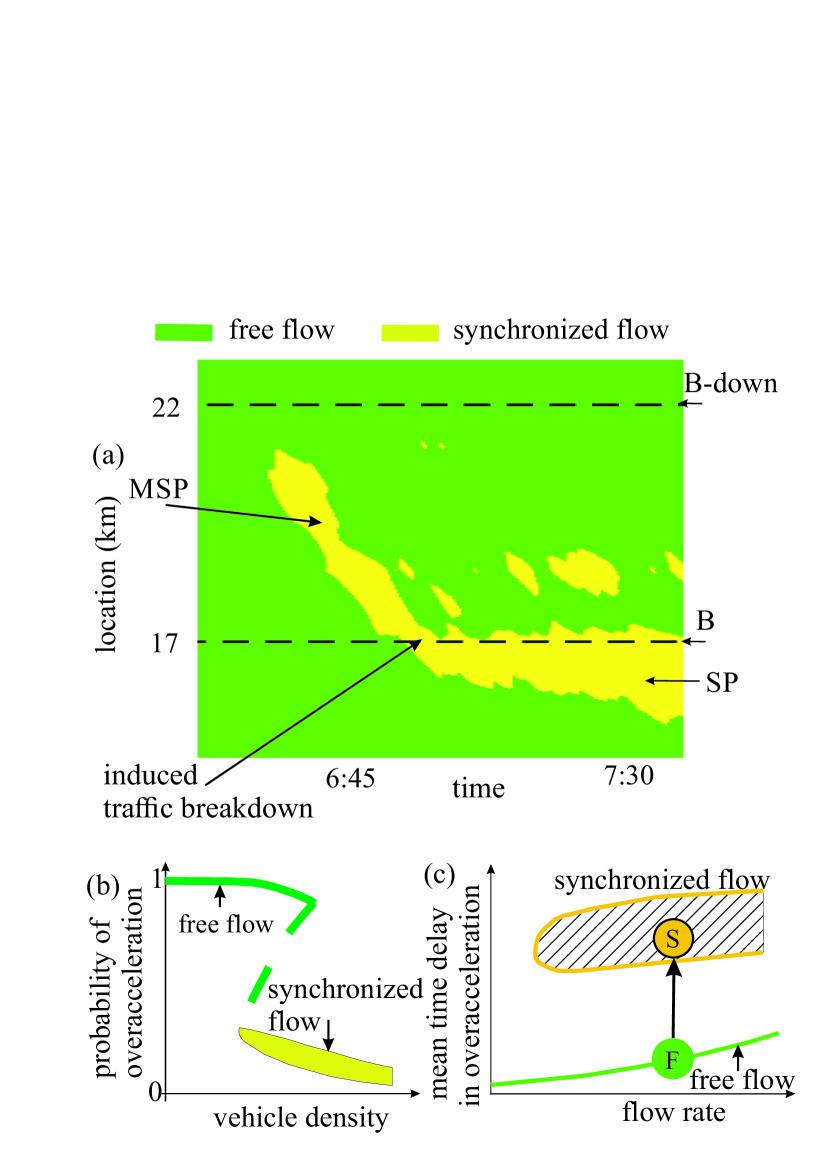
Figure 1: Hypothesis of three-phase traffic theory about the discontinuous character of driver overacceleration OA . (a) Empirical nucleation nature of traffic breakdown (F$\rightarrow$S transition) at bottlenecks. Speed data presented in space and time with averaging method described in Sec. C.2 of Ref. TomTom were measured with road detectors installed along road: A moving synchronized flow pattern (MSP) that has emerged at downstream bottleneck (B-down) while propagating upstream induces F$\rightarrow$S transition (induced traffic breakdown) leading to emergence of a synchronized flow pattern (SP) at upstream bottleneck (B); adapted from KernerBook1 ; KernerBook2 ; KernerBook3 ; KernerBook4 . (b), (c) Qualitative vehicle density-dependence of driver overacceleration probability per a time interval (b) and equivalent presentation of (b) as a discontinuous flow-rate dependence of the mean time-delay in overacceleration (c): At given initial traffic parameters (e.g., at given flow rates at traffic network boundaries), during F$\rightarrow$S phase transition the probability of overacceleration drops abruptly whereas the mean time delay in overacceleration jumps abruptly; F and S are states of free flow and synchronized flow, respectively.

The discontinuous character of overacceleration is not solely the feature of human-driving vehicles. Indeed, in traffic flow consisting of 100$\%$ of automated-driving vehicles there is also a discontinuity in the probability of overacceleration of the automated-driving vehicles that is the cause for the nucleation nature of the F$\rightarrow$S transition at the bottleneck Kerner2023C . Therefore, for both human-driving and automated-driving vehicles we can generalize the definition of the term overacceleration as follows:

• Vehicle acceleration behavior that causes the free flow metastability with respect to the F$\rightarrow$S transition at the bottleneck is called vehicle overacceleration.

The discontinuous character of overacceleration is a basic feature of overacceleration [Fig. 1(b)] . In general, for both human-driving and automated-driving vehicles moving in traffic flow, the behavioral origin of vehicle overacceleration is related to the vehicle’s desire to move in free flow.

The term overacceleration should distinguish vehicle overacceleration behaviors that do result in the free flow metastability with respect to the F$\rightarrow$S transition at the bottleneck from usual vehicle acceleration behaviors that do not cause the free flow metastability.

The overacceleration effect is in a spatiotemporal competition with the opposite effect of speed adaptation related to deceleration of the vehicle that approaches a slower moving preceding vehicle. Contrary to overacceleration, speed adaptation describes the tendency from free flow to congested traffic at the bottleneck: Only if the overacceleration effect is on average stronger than speed adaptation, free flow remains at the bottleneck; otherwise, speed adaptation leads to the F$\rightarrow$S transition at the bottleneck.

In stochastic three-phase traffic flow models KKl ; OA_Stoch ; Kerner2015_SF ; TPACC , overacceleration has been described on average through model fluctuations. Although in KKl ; OA_Stoch ; Kerner2015_SF ; TPACC many empirical spatiotemporal features of traffic breakdown and resulting congested patterns have been explained , however, microscopic characteristics of overacceleration is difficult to disclose through a study of the stochastic models. In Kerner2023B , a simple deterministic model of overacceleration in a road lane has been introduced that exhibits the discontinuous character. In this model, overacceleration exceeds zero only when the vehicle speed is equal or larger than a threshold synchronized vehicle speed. This overacceleration model explains the empirical nucleation nature of traffic breakdown. However, this simple overacceleration model Kerner2023B cannot alone explain a possible diversity of microscopic features of the effect of vehicle overacceleration on traffic flow.

Indeed, a microscopic theory of the effect of vehicle overacceleration on traffic flow developed in this paper will show that there are other microscopic mechanisms of overacceleration. Moreover, we will find that there is a cooperation between the different mechanisms of overacceleration, which appear to be very essential for the occurrence of the critical nucleus for the F$\rightarrow$S transition as well as for an S$\rightarrow$F instability.

The paper is organized as follows. A deterministic three-phase traffic flow model used for simulations has been developed in Sec. II, overacceleration mechanisms caused by safety acceleration on single-lane road are studied in Sec. III, a cooperation of different mechanisms of overacceleration is the subject of Sec. IV, the effect of overacceleration in a road lane on overacceleration through lane-changing is studied in Sec. V, a theory of the critical nucleus for spontaneous traffic breakdown is presented in Sec. VI, a proof of the effect of vehicle overacceleration on traffic flow is given in Sec. VII, an S$\rightarrow$F instability on two-lane road caused by overacceleration cooperation is analyzed in Sec. VIII. In Sec. IX, we explain what microscopic behaviors of vehicle motion are the cause of overacceleration (Sec. IX.1), generalize the model for moving jam simulations (Sec. IX.2), discuss vehicle overacceleration versus vehicle overdeceleration (Secs. IX.3 and IX.4) as well as formulate conclusions (Sec. IX.5).

II Microscopic model of vehicular traffic

II.1 Basic three-phase traffic flow model

As a basic model for vehicle motion, we apply Kerner’s model of Ref. Kerner2023B . In the microscopic deterministic traffic flow model, vehicle acceleration/deceleration $a$ in a road lane is described by a system of equations:

$$a=a_{\rm OA}+K_{\Delta v}\Delta v\ \textrm{at $g_{\rm safe}\leq g\leq G$},$$ (1)

$$a=a_{\rm G}\ \textrm{at $g>G$},$$ (2)

$$a=a_{\rm safety}(g,v,v_{\ell})\ \textrm{at $g<g_{\rm safe}$},$$ (3)

where overacceleration $a_{\rm OA}$ in a road lane is given by equation:

$$a_{\rm OA}=\alpha\Theta(v-v_{\rm syn}),$$ (4)

$v$ is the vehicle speed, $0\leq v\leq v_{\rm free}$, $v_{\rm free}$ is a maximum vehicle speed; $\alpha$ is a coefficient of overacceleration; $\Theta(z)=0$ at $z<0$ and $\Theta(z)=1$ at $z\geq 0$; $v_{\rm syn}$ is a given synchronized flow speed ($v_{\rm syn}<v_{\rm free}$); $g$ is a space gap to the preceding vehicle, $g=x_{\ell}-x-d$, $x$ and $x_{\ell}$ are, respectively, the coordinates of the vehicle and the preceding vehicle, $d$ is the vehicle length;

$$\Delta v=v_{\ell}-v,$$

$v_{\ell}$ is the speed of the preceding vehicle; $K_{\Delta v}$ is a positive dynamic coefficient; $G$ is a synchronization space gap; $g_{\rm safe}$ is a safe space gap; $a_{\rm safety}(g,v,v_{\ell})$ is a safety vehicle acceleration ; $a_{\rm G}$ is vehicle acceleration at large space gaps; vehicle acceleration and speed are limited by maximum acceleration $a=a_{\rm max}$ and $v=v_{\rm free}$, respectively.

II.2 Vehicle acceleration at large space gaps

In Kerner2023B , to prove the metastability of free flow at a bottleneck through the effect of overacceleration without vehicle overdeceleration, for simplification of Eq. (2) we have set $a_{\rm G}$ as constant value: $a_{\rm G}=a_{\rm max}$ . However, to develop a microscopic theory of the effect of vehicle overacceleration on traffic flow, the model should be able to capture a variety of real traffic scenarios. Therefore, we get:

$$a_{\rm G}(g,v,v_{\ell})=a_{\rm OA}+K_{1}(g-v\tau_{\rm G})+K_{2}\Delta v,$$ (5)

where $a_{\rm OA}$ is given by Eq. (4); $K_{1}$ and $K_{2}$ are positive dynamic coefficients. Note that the two last terms in the right hand of Eq. (5) is well-known Helly’s formula Helly  . In particular, through the use of the term $K_{2}\Delta v$ of Helly’s formula we take into account situations at which a vehicle that initial gap $g>G$ approaches a slower moving preceding vehicle.

II.3 Space-gap dependence of overacceleration

In numerical simulations of (1)–(4) made in Kerner2023B , for simplification the coefficient of overacceleration $\alpha$ in (4) has been chosen a constant. However, it is physically more realistic to assume that $\alpha$ in (4) should depend on the space-gap $g$. In particular, within the space-gap range $g_{\rm safe}\leq g\leq G$ overacceleration should be the larger, the larger the space-gap $g$. Indeed, the less the difference $g-g_{\rm safe}$ between the space-gap and the safe space-gap, the smaller should be the probability of overacceleration. Therefore, in (4) we get

$$\alpha=\left\{\begin{array}[]{ll}\alpha_{0}\ \textrm{at $g>G$},\\ (\alpha_{0}-\alpha_{1})\Biggl{(}\frac{g-g_{\rm safe}}{G-g_{\rm safe}}\Biggr{)}^{k}+\alpha_{1}\ \textrm{at $g_{\rm safe}\leq g\leq G$},\\ \end{array}\right.$$ (6)

where $k$, $\alpha_{0}$, and $\alpha_{1}$ are positive model parameters, $\alpha_{0}>\alpha_{1}$.

II.4 Safety vehicle acceleration

Eq. (3) describes safety vehicle acceleration that should prevent collisions between vehicles at small space gaps $g<g_{\rm safe}$. There are many concepts developed in standard traffic flow models GM_Com1 ; GM_Com2 ; GM_Com3 ; KS ; KS1 ; KS2 ; KS4 ; Newell1961 ; Newell ; Gipps1981 ; Gipps1986 ; Wiedemann ; Nagel_S ; Bando_1 ; Bando ; Bando_2 ; Bando_3 ; Nagatani_1 ; Nagatani_2 ; Treiber ; Jiang2001 ; KK1994 ; Krauss ; Barlovic ; Gartner ; Barcelo ; Elefteriadou ; DaihengNi ; Chowdhury ; Helbing ; Nagatani_R ; Nagel ; Treiber-Kesting ; Schadschneider ; Helly that can be used for safety vehicle acceleration $a_{\rm safety}(g,v,v_{\ell})$. In Kerner2023B , Helly’s formula Helly has been used for safety vehicle acceleration: $a_{\rm safety}(g,v,v_{\ell})=K_{g}(g-g_{\rm safe})+K_{v}\Delta v$, where $K_{g}$ and $K_{v}$ are positive dynamic coefficients. However, from the analysis of Helly’s formula made in Kerner2023C , we know that in some traffic situations at a large enough negative speed difference $\Delta v$, specifically by lane changing at low enough vehicle speeds, vehicle collisions can be possible .

To avoid vehicle collisions, for safety acceleration $a_{\rm safety}(g,v,v_{\ell})$ in (3) we apply ideas of dynamic breaking strategies of General Motors car-following model of Herman, Gazis, Montroll, Potts, Rothery, and Chandler GM_Com1 ; GM_Com2 ; GM_Com3 ; Gazis , in which at $\Delta v<0$ vehicle deceleration is proportional to the term

$$\frac{v\tau_{\rm safe}}{g}\Delta v,$$

where $\tau_{\rm safe}$ is a safe time headway. This idea of the GM-model GM_Com1 ; GM_Com2 ; GM_Com3 ; Gazis insures that the dynamic vehicle breaking should be the stronger, the lower the space gap $g$ between vehicles is. Accordingly, instead of Helly’s formula we get

$$a_{\rm safety}(g,v,v_{\ell})=K_{3}(g-g_{\rm safe})+K_{4}(g,v,\Delta v)\Delta v,$$ (7)

where

$$K_{4}=\left\{\begin{array}[]{ll}K^{(1)}_{4}\ \textrm{at $\Delta v>0$},\\ K^{(2)}_{4}\frac{v\tau_{\rm safe}}{g}\ \textrm{at $\Delta v\leq 0$}.\\ \end{array}\right.$$ (8)

$K_{3}$, $K^{(1)}_{4}$, and $K^{(2)}_{4}$ are positive dynamic coefficients. To make vehicle deceleration without jumps at $\Delta v<0$, when the space gap $g$ intersects boundaries $G$ and $g_{\rm safe}$ of the indifferent zone, in (1) we apply 

$$K_{\Delta v}=\left\{\begin{array}[]{ll}K_{2}\ \textrm{at $\Delta v>0$},\\ K^{(1)}_{\Delta v}\ \textrm{at $\Delta v\leq 0$},\\ \end{array}\right.$$ (9)

where

$$K^{(1)}_{\Delta v}=\Biggl{(}K_{2}-K^{(2)}_{4}\frac{v\tau_{\rm safe}}{g}\Biggr{)}\Biggl{(}\frac{g-g_{\rm safe}}{G-g_{\rm safe}}\Biggr{)}+K^{(2)}_{4}\frac{v\tau_{\rm safe}}{g}.$$ (10)

In addition to traffic flow consisting of human-driving vehicles, the model (1)–(10) is also applicable for traffic flow consisting of automated-driving vehicles as well as for mixed traffic flow in which automated-driving vehicles move with the use of three-phase adaptive cruise control (TPACC) TPACC ; TPACC2  .

II.5 Models of lane-changing and on-ramp bottleneck

We use well-known incentive lane changing rules from the right to left lane R$\rightarrow$L (11) and from the left to right lane L$\rightarrow$R (12) as well as well-known safety conditions (13) (see, e.g., Nagel1998 )

$$R\rightarrow L:v^{+}(t)\geq v_{\ell}(t)+\delta_{1}\ {\rm and}\ v(t)\geq v_{\ell}(t),$$ (11)

$$L\rightarrow R:v^{+}(t)\geq v_{\ell}(t)+\delta_{2}\ {\rm or}\ v^{+}(t)\geq v(t)+\delta_{2},$$ (12)

$$g^{+}(t)\geq\ v(t)\tau_{2},\quad g^{-}(t)\geq\ v^{-}(t)\tau_{1},$$ (13)

at which a vehicle changes to the faster target lane with the objective to pass a slower vehicle in the current lane if time headway to preceding and following vehicles in the target lane are not shorter than some given safety time headway $\tau_{1}$ and $\tau_{2}$. In (11)–(13), superscripts $+$ and $-$ denote, respectively, the preceding and the following vehicles in the target lane; $\tau_{1}$, $\tau_{2}$, $\delta_{1}$, $\delta_{2}$ are positive constants .

Open boundary conditions are applied. At the beginning of the two-lane road $x=0$ vehicles are generated one after another in each of the lanes of the road at time instants $t^{(k)}=k\tau_{\rm in}$, $k=1,2,\ldots$, where $\tau_{\rm in}=1/q_{\rm in}$, $q_{\rm in}$ is a given time-independent flow rate per road lane. The initial vehicle speed is equal to $v_{\rm free}$. After the vehicle has reached the end of the road $x=L$ it is removed. Before this occurs, the farthest downstream vehicle maintains its speed and lane.

In the on-ramp model, there is a merging region of length $L_{\rm m}$ in the right lane that begins at location $x=x_{\rm on}$ within which vehicles can merge from the on-ramp. Vehicles are generated at the on-ramp one after another at time instants $t^{(m)}=m\tau_{\rm on}$, $m=1,2,\ldots$, where $\tau_{\rm on}=1/q_{\rm on}$, $q_{\rm on}$ is the on-ramp inflow rate. To reduce a local speed decrease occurring through the vehicle merging at the on-ramp bottleneck, vehicles merge with the speed of the preceding vehicle $v^{+}$ at a middle location $x=(x^{+}+x^{-})/2$ between the preceding and following vehicles in the right lane, when the space gap between the vehicles exceeds some safety value $g^{\rm(min)}_{\rm target}=\lambda_{\rm b}v^{+}+d$, i.e., some safety condition $x^{+}-x^{-}-d>g^{\rm(min)}_{\rm target}$ should be satisfied. In accordance with these merging conditions, the space gap for a vehicle merging between each pair of consecutive vehicles in the right lane is checked within merging region $L_{\rm m}$, starting from the upstream boundary of the merging region. If there is such a pair of consecutive vehicles, the vehicle merges onto the right lane; if there is no pair of consecutive vehicles, for which the safety condition is satisfied at the current time step, the procedure is repeated at the next time step, and so on.

Vehicle motion is found from a system of equations $a^{\ast}=\min(a,a_{\rm max})$, $dv^{\ast}/dt=a^{\ast}$, $v=\max(0,\min(v^{\ast},v_{\rm free}))$ that results from conditions $0\leq v\leq v_{\rm free}$, and $dx/dt=v$ solved with the second-order Runge-Kutta method with time step $10^{-2}$ s.

In the main text of the paper, we use simple speed-functions $G(v)$ and $g_{\rm safe}(v)$:

$$G(v)=v\tau_{\rm G},\quad g_{\rm safe}(v)=v\tau_{\rm safe},$$ (14)

where $\tau_{\rm G}$ is a synchronization time headway. We choose dynamic coefficients $K_{3}$ and $K_{4}$ in (7), (8) at which under conditions (14) no classical traffic flow instability (no string instability) can occur. Respectively, no wide moving jams (and no cases at which $v\rightarrow 0$) can occur in synchronized flow of the model (1)–(14).

III Overacceleration caused by safety acceleration

We show that in addition with the overacceleration mechanisms in a road lane (4) Kerner2023B and through lane-changing Kerner2023C there are other mechanisms of overacceleration in the road lane caused by safety acceleration $a_{\rm safety}$. To understand this, we should consider the overacceleration mechanisms separately from each other. With this aim, in Sec. III we consider a single-lane road and neglect overacceleration (4) of Ref. Kerner2023B , i.e., in (4) we get

$$\alpha=0.$$ (15)

III.1 No overacceleration – no nucleation nature of F$\rightarrow$S transition

First, we consider a case in which under condition (15) safety acceleration behavior does not act as overacceleration (Fig. 2): There is no acceleration behavior that could cause the free flow metastability with respect to traffic breakdown at the bottleneck. Indeed, in Fig. 2, contrary to empirical data, traffic breakdown does not exhibit the nucleation nature.

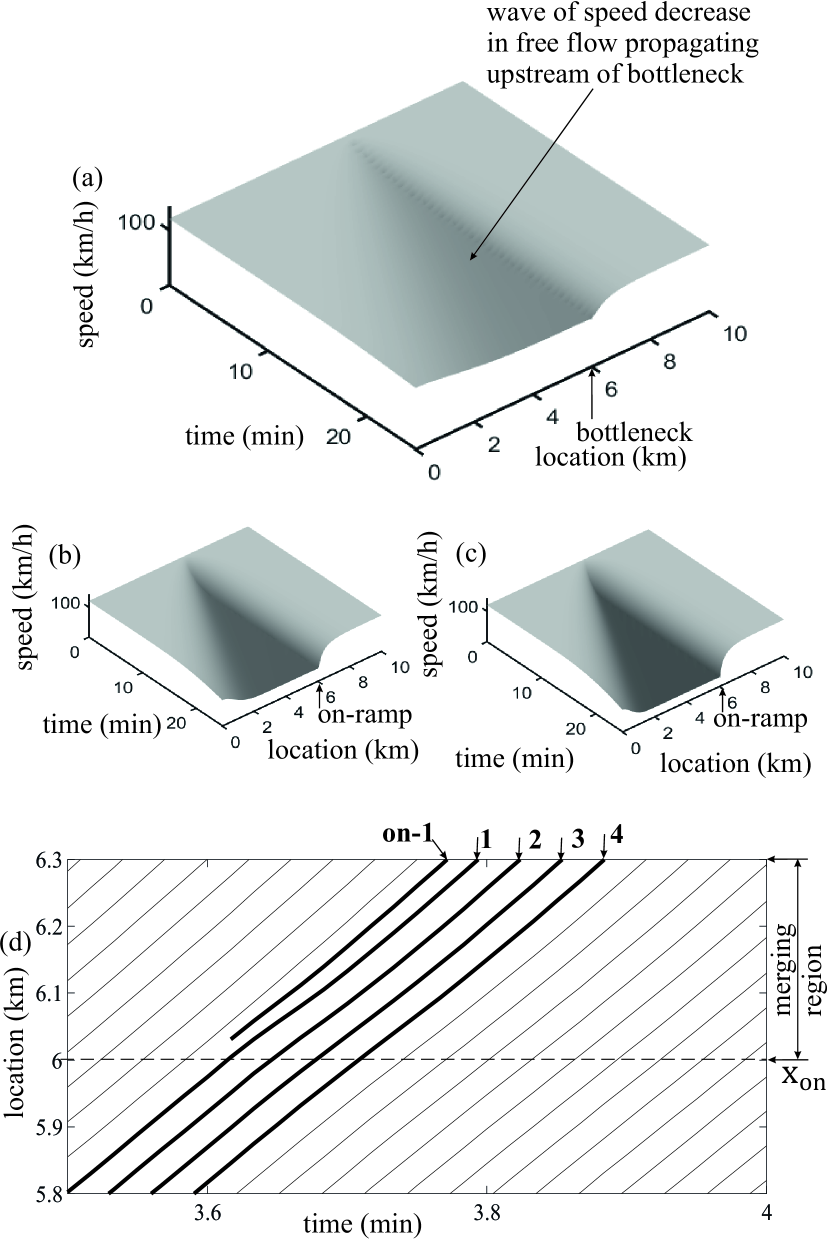
Figure 2: Explanation to $``$no overacceleration – no nucleation nature of F$\rightarrow$S transition”. Simulations of model (1)–(10), (14), (15) at $q_{\rm in}=$ 2000 vehicles/h and different values of on-ramp inflow rate $q_{\rm on}$ at coefficient of overacceleration $\alpha=$ 0 (15), i.e., in (1) and (5) $a_{\rm OA}=$ 0. (a)–(c) Speed in space and time: (a) $q_{\rm on}=$ 100 vehicles/h, (b) $q_{\rm on}=$ 350 vehicles/h, (c) $q_{\rm on}=$ 500 vehicles/h. (d) Simulated vehicle trajectories in some time interval related to (a). Other model parameters: $v_{\rm free}=$ 120 km/h, $\tau_{\rm safe}=$ 1 s, $\tau_{\rm G}=$ 2 s, $v_{\rm syn}=$ 80 km/h, $d=$ 7.5 m, $a_{\rm max}=$ 2.5 $\rm m/s^{2}$, $K_{1}=0.3\ s^{-2}$, $K_{2}=K^{(1)}_{4}=0.6\ s^{-1}$, $K_{3}=0.5\ s^{-2}$, $K^{(2)}_{4}=1\ s^{-1}$, $L=$ 10 km, $x_{\rm on}=$ 6 km, $\lambda_{\rm b}=$ 0.2 s, $L_{\rm m}=$ 0.3 km.

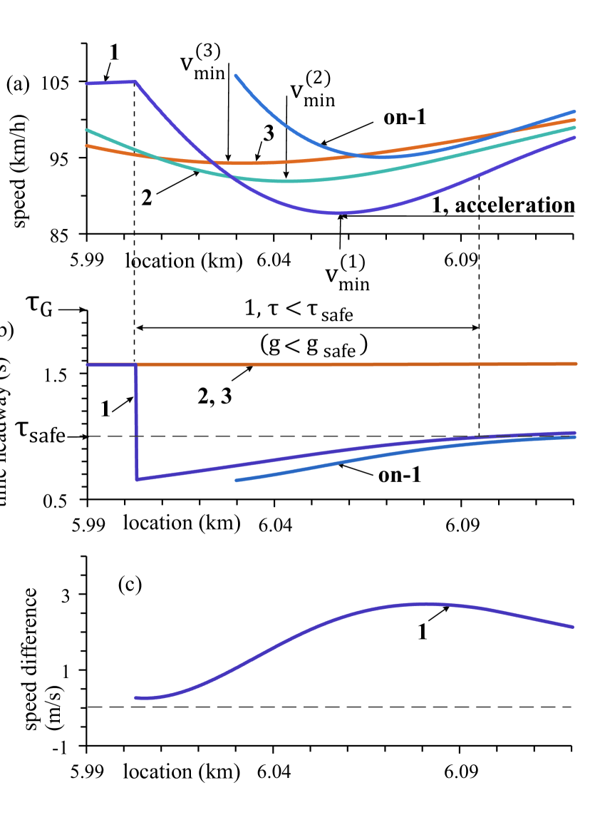
Figure 3: Continuation of Fig. 2(d). (a), (b) Location-functions of speed (a) and time-headway (b) of some vehicles. (c) Location-function of speed difference $\Delta v=v^{\rm(on-1)}-v^{(1)}$ between speeds of vehicles on-1 and 1. Vehicle numbers are the same as those in Fig. 2(d), respectively.

To explain this, we consider Fig. 3. After vehicle on-1 has merged from the on-ramp onto the main road [Fig. 2(d)], time-headway of vehicle 1 following vehicle on-1 on the main road becomes smaller than safe time-headway $\tau_{\rm safe}$ [Fig. 3(b)]. Therefore, according to Eqs. (7) and (8), vehicle 1 should decelerate strongly resulting in deceleration of following vehicles 2 and 3 [Fig. 3(a)]. Deceleration of vehicles 2 and 3 is realized within the indifferent zone for car-following $g_{\rm safe}\leq g\leq G$ [$\tau_{\rm safe}\leq\tau\leq\tau_{\rm G}$ in Fig. 3(b)] in accordance with equation

$$a=K_{\Delta v}\Delta v\ \textrm{at $g_{\rm safe}\leq g\leq G$}$$ (16)

resulting from Eqs. (1) and (15). Eq. (16) describes vehicle speed adaptation to the speed of the preceding vehicle: After vehicle 1 begins to decelerate, following vehicle 2 decelerates while adapting its speed to the speed of vehicle 1; the deceleration of vehicle 2 leads to the deceleration of vehicle 3, and so on. Locations of the minimum speed of vehicles 2, 3, $\ldots$ (e.g., $v^{(2)}_{\rm min}$ and $v^{(3)}_{\rm min}$) are upstream of the location of the minimum speed of vehicle 1 [Fig. 3(a)]. This explains the occurrence of the wave of a speed decrease propagating upstream of the bottleneck [Fig. 2(a)]; at a given $q_{\rm in}$, the larger the on-ramp inflow rate $q_{\rm on}$, the lower the speed in this congested traffic [Figs. 2(a) and 2(c)]. Such spontaneous propagation congestion upstream of the on-ramp bottleneck is well-known in standard traffic flow theory . In accordance with overacceleration definition (Sec. I), in the model used in Fig. 2, in which no nucleation nature of traffic breakdown is realized, safety acceleration [labeled by $``$1, acceleration” in Fig. 3(a)] cannot be considered overacceleration.

III.2 Overacceleration under decrease in time-headway between vehicles in free flow

We consider the same model (1)–(8), (14), (15) as used in Fig. 2. However, we decrease time-headway between vehicles in free flow through an increase in the flow rate on the main road $q_{\rm in}$. Then, rather than the speed wave propagating upstream of the bottleneck [Fig. 2(a)], the wave of a speed decrease propagating downstream of the bottleneck occurs [Fig. 4(a)]. As a result, free flow remains upstream of the bottleneck. Moreover, if in simulations shown in Fig. 4(a) at some time instant $T_{\rm ind}$ we apply a short-time impulse of addition large enough on-ramp inflow $\Delta q_{\rm on}$, synchronized flow propagating upstream has been induced in the initial free flow at the bottleneck [Fig. 4(b)]. Thus, contrary to Fig. 2, in Fig. 4 free flow becomes metastable with respect to the F$\rightarrow$S transition.

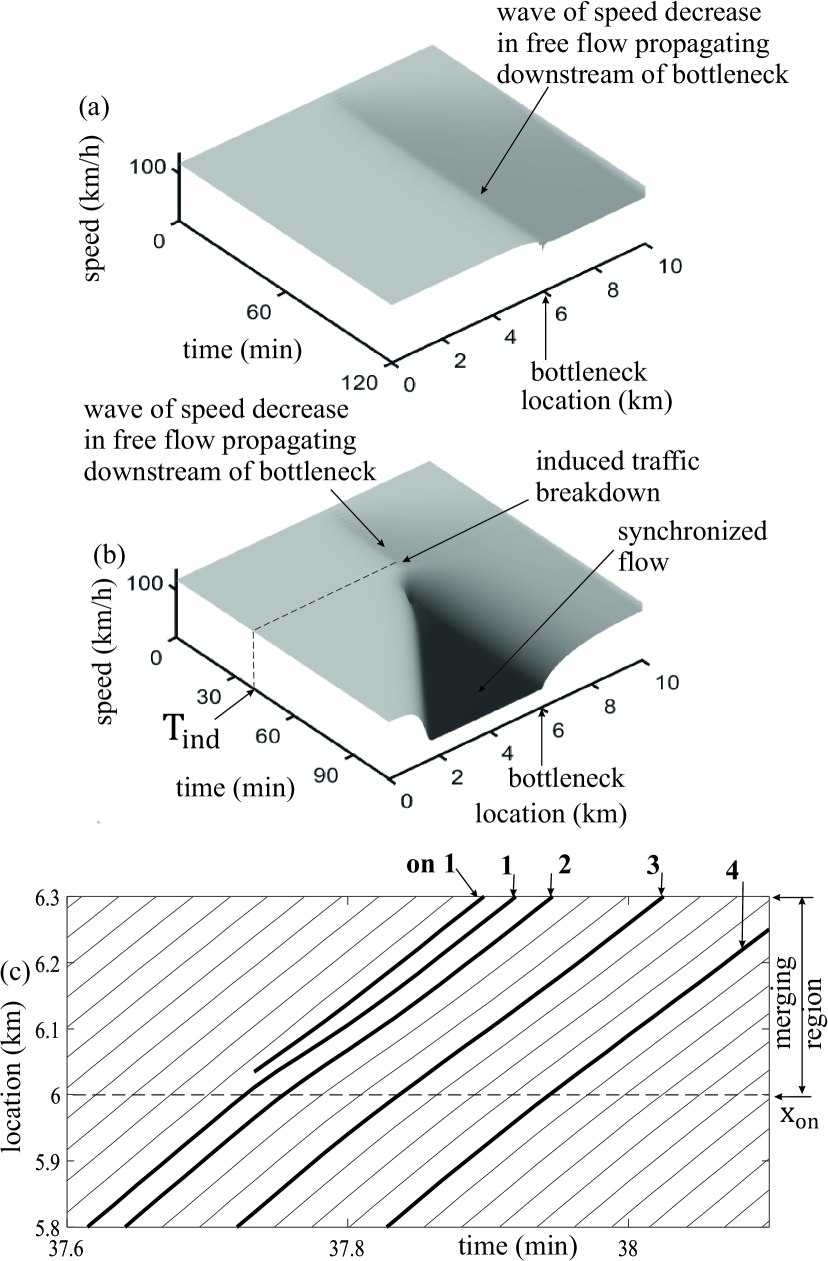
Figure 4: Overacceleration in single-lane road under decrease in time-headway in free flow upstream of on-ramp bottleneck. Simulations of the model (1)–(10), (14), (15) under the same model parameters as those in Fig. 2(a) with the exceptions of the choice of another coefficient $K^{(2)}_{4}=0.8\ s^{-1}$ and a higher flow rate $q_{\rm in}=$ 2250 vehicles. (a), (b) Speed in space and time at $q_{\rm on}=$ 35 vehicles/h. In (b), traffic breakdown has been induced in free flow at $T_{\rm ind}=$ 40 min through application of addition on-ramp inflow impulse $\Delta q_{\rm on}=$ 500 vehicles/h of duration $\Delta t=$ 1 min. (c) Some of simulated vehicle trajectories within local speed decrease in free flow at bottleneck at time $t<T_{\rm ind}$.

To understand the crucial difference between Figs. 2 and 4, first we note that there are common features in behaviors of vehicles on-1 and 1 following each other [Figs. 3 and 5]: After vehicle on-1 has merged from the on-ramp [Figs. 2(d) and 4(c)], space-gap of vehicle 1 becomes smaller than safe space-gap $g_{\rm safe}$ (i.e., time-headway is shorter than $\tau_{\rm safe}$) [Figs. 3(b) and 5(b)]. Therefore, according to Eqs. (7) and (8), vehicle 1 should decelerate strongly [Figs. 3(a) and 5(a)]. Shortly later, although condition $g<g_{\rm safe}$ is still satisfied, this braking of vehicle 1 changes to its acceleration at location labeled by $v^{(1)}_{\rm min}$ in Figs. 3(a) and 5(a). This safety acceleration of vehicle 1 under condition $g<g_{\rm safe}$ occurs because the speed difference $\Delta v=v^{(on-1)}-v^{(1)}$ between vehicles on-1 and 1 becomes a large enough value [Figs. 3(c) and 5(c)] leading to condition

$$a_{\rm safety}=K_{3}(g-g_{\rm safe})+K^{(1)}_{4}\Delta v>0\ {\rm at}\ g<g_{\rm safe}.$$ (17)

The crucial difference between Figs. 2 and 4 is associated with behaviors of vehicles 2, 3, and 4 that follow vehicle 1 on the main road [Figs. 3(a) and 5(a)]. In comparison with Fig. 3(a), in Fig. 5(a) time-headway between vehicles in free flow are considerably shorter. As a result, locations of the speed minimum of vehicles 2, 3, and 4 ($v^{(2)}_{\rm min}$, $v^{(3)}_{\rm min}$, and $v^{(4)}_{\rm min}$, respectively) following vehicle 1 are downstream of the beginning of the on-ramp merging region $x_{\rm on}$ [Figs. 5(a) and 5(b)]. Moreover, the distances between the location of the minimum speed of vehicle 1 [$v^{(1)}_{\rm min}$ in Fig. 5(a)] and locations of the minimum speeds of the following vehicles increase with the vehicle number [Fig. 5(a)]. This explains the occurrence of the wave of a speed decrease propagating downstream of the bottleneck [Fig. 4(a)]. This wave results from safety acceleration of vehicle 1 described by Eq. (17). Free flow is in a metastable state with respect to the F$\rightarrow$S transition at the bottleneck [Fig. 4(b)]. Thus, in accordance with the overacceleration definition, safety acceleration should be considered overacceleration [$``$1, overacceleration” in Fig. 5(a)].

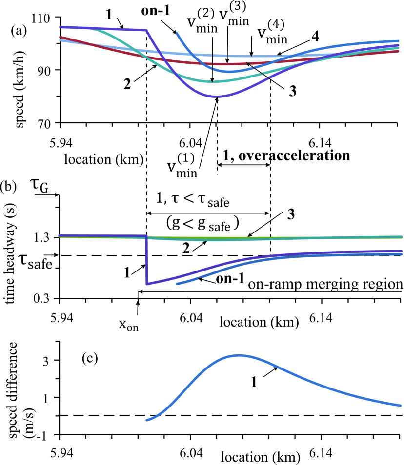
Figure 5: Continuation of Fig. 4(c). (a), (b) Location-functions of speed (a) and time-headway (b) of some vehicles. (c) Location-function of speed difference $\Delta v=v^{(on-1)}-v^{(1)}$ between speeds of vehicles on-1 and 1. Vehicle numbers are labeled by the same numbers as those in Fig. 4(c).

III.3 Overacceleration under increase in time-headway between vehicles in free flow above synchronization time-headway

Under condition (15) and at the same flow rates $q_{\rm in}$ and $q_{\rm on}$ as those in Fig. 2(b), another overacceleration mechanism caused by safety acceleration has been found (Fig. 6). This overacceleration mechanism is realized under condition

$$g_{\rm free}>G,\ {\rm i.e.,}\ \tau_{\rm free}>\tau_{\rm G},$$ (18)

where $g=g_{\rm free}=\frac{v_{\rm free}}{q_{\rm in}}-d$ and $\tau=\tau_{\rm free}=g_{\rm free}/v_{\rm free}$ are, respectively, the average space-gap $g$ and time-headway $\tau$ between vehicles in free flow moving at the maximum speed $v_{\rm free}$. Indeed, under condition (18) rather than congestion propagation upstream of the bottleneck [Fig. 2(b)], free flow remains at the bottleneck. In this free flow, only a small speed decrease localized at the bottleneck is realized [Fig. 6(a)]. This free flow is in a metastable state with respect to an F$\rightarrow$S transition at the bottleneck [Fig. 6(b)]. To understand the physics of this overacceleration effect, first we should note that there are common features in behaviors of vehicles on-1 and 1 in Figs. 3 and 7. These common features are exactly the same as those explained above in Sec. III.2 when we have compared Figs. 3 and 5. In particular, under condition $g<g_{\rm safe}$ safety acceleration of vehicle 1 [Figs. 7(a) and 7(b)] occurs in accordance with Eq. (17).

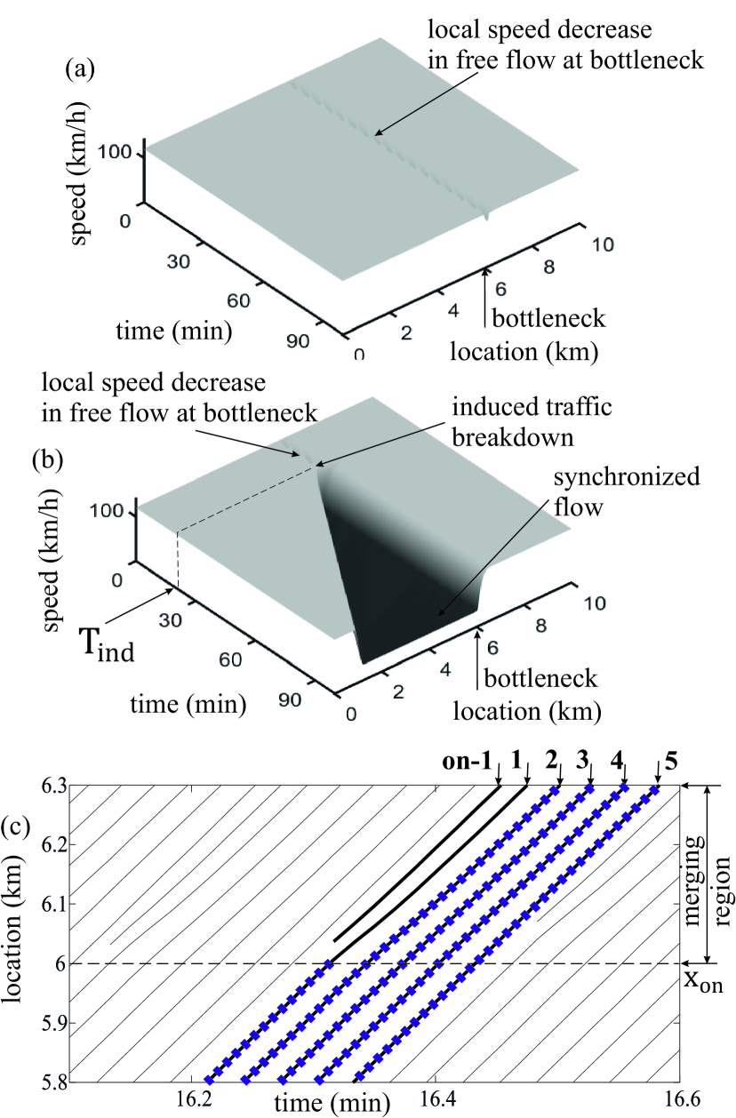
Figure 6: Induced traffic breakdown on single-lane road with on-ramp bottleneck under condition (18). Simulations of model (1)–(10), (14), (15) at $\tau_{\rm G}=$ 1.4 s, $q_{\rm in}=$ 2000 vehicles/h, and $q_{\rm on}=$ 350 vehicles/h. Other model parameters are the same as those in Fig. 2(a). (a), (b) Speed in space and time: Local speed decrease at bottleneck in free flow (a) and synchronized flow pattern (SP) (b) induced in free flow in (a) at $T_{\rm ind}=$ 20 min through application of addition on-ramp inflow impulse $\Delta q_{\rm on}=$ 600 vehicles/h of duration $\Delta t=$ 1 min. (c) Some of simulated vehicle trajectories within local speed decrease in free flow at bottleneck at time $t<T_{\rm ind}$; parts of trajectories within which condition $g>G$ is satisfied are marked through colored blue rectangles.

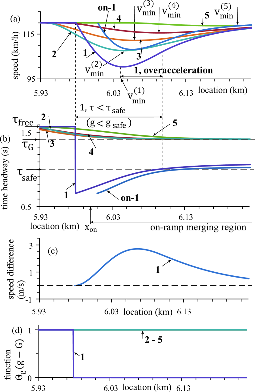
Figure 7: Continuation of Fig. 6(c). (a), (b) Location-functions of speed (a) and time-headway (b) of some vehicles. (c) Location-function of speed difference $\Delta v=v^{\rm(on-1)}-v^{(1)}$ between speeds of vehicles on-1 and 1. (d) Dependencies of function $\Theta_{\rm g}(g-G)$ on road location for vehicles 1–5, where $\Theta_{\rm g}(z)=0$ at $z<0$ and $\Theta(z)=1$ at $z\geq 0$. Vehicle numbers are labeled by the same numbers as those in Fig. 6(c).

There is the following crucial difference between the case under consideration (Fig. 6) and the cases studied in Secs. III.1 and III.2 [Figs. 2 and 4]: In Figs. 2 and 4, deceleration and acceleration of the vehicles 2 and 3 following vehicle 1 are realized within the indifferent zone for car-following $g_{\rm safe}\leq g\leq G$ [region $\tau_{\rm safe}\leq\tau\leq\tau_{\rm G}$ in Figs. 3(b) and 5(b)], i.e., it corresponds to solutions of Eq. (16). Contrarily, under condition (18) for which Fig. 6 is valid, vehicles 2–5 following vehicle 1 [Fig. 7(b)] decelerate and accelerate in accordance with Eqs. (5) and (15) corresponding to solutions of equation

$$a_{\rm G}=K_{1}(g-v\tau_{\rm G})+K_{2}\Delta v\ {\rm at}\ g>v\tau_{\rm G}.$$ (19)

When vehicle 1 decelerates, then both Eqs. (16) and (19) describe speed adaptation of following vehicles to the speed of vehicle 1. However, as long as condition $g>v\tau_{\rm G}$ is satisfied, due to positive term $K_{1}(g-v\tau_{\rm G})$ in Eq. (19), at the same negative speed difference $\Delta v$ in Eqs. (16) and (19) the deceleration and respective speed decrease of vehicles 2–5 in Fig. 7(a) are considerable lower than those of vehicles 2 and 3 in Fig. 3(a).

As mentioned in Sec. III.1, a large speed decrease of vehicles 2 and 3 in Fig. 3(a) occurs already upstream of the bottleneck leading to the wave of a speed decrease propagating upstream of the bottleneck [Fig. 2(a)]. Contrarily, due to a weaker deceleration (19), vehicles 2–5 in Fig. 7(a) reach the bottleneck while moving still in free flow, i.e., free flow remains at the bottleneck. Deceleration of vehicles 2–5 causes only a weak wave of a speed decrease propagating downstream of the bottleneck. Indeed, the locations of the speed minimum of vehicles 2–5 [$v^{(2)}_{\rm min}$, $v^{(3)}_{\rm min}$, $v^{(4)}_{\rm min}$, and $v^{(5)}_{\rm min}$ in Fig. 7(a), respectively] following vehicle 1 are downstream of the location of the speed minimum of vehicle 1 [$v^{(1)}_{\rm min}$ in Fig. 7(a)]; however, contrary to Fig. 4(a), due to the weak deceleration of vehicle 2–5 the wave disappears almost fully at a short distance downstream of the beginning of the on-ramp [Fig. 7(a)]. For this reason, a speed decrease caused by vehicle merging from the on-ramp can be considered as a local speed decrease at the bottleneck [$``$local speed decrease” in Fig. 6(a)].

In Fig. 6, contrary to Fig. 2, safety acceleration does cause the metastability of free flow with respect of F$\rightarrow$S transition at the bottleneck. Thus, due to condition (18), safety acceleration (7), (8) becomes overacceleration [$``$1, overacceleration” in Fig. 7(a)].

IV Cooperation of different mechanisms of overacceleration

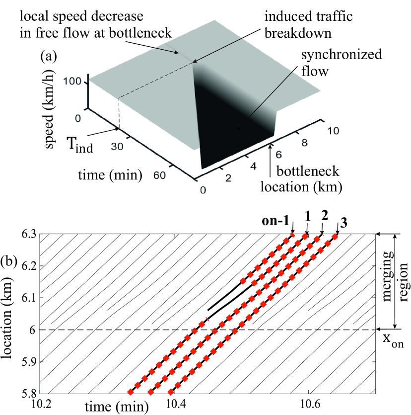
Figure 8: Simulations of cooperation of different mechanisms of overacceleration on single-lane road. Induced traffic breakdown on single-lane road with on-ramp bottleneck. Simulations of model (1)–(10), (14) with model parameters: $\alpha_{0}=$ 2 $\rm m/s^{2}$, $\alpha_{1}=$ 0.1 $\rm m/s^{2}$, $k=$ 1, $\tau_{\rm G}=$ 1.4 s, $q_{\rm in}=$ 2000 vehicles/h, $q_{\rm on}=$ 800 vehicles/h; other model parameters are the same as those in Fig. 2. (a) Speed in space and time: Local speed decrease at bottleneck in free flow and synchronized flow pattern (SP) induced in the free flow at $T_{\rm ind}=$ 20 min through application of addition on-ramp inflow impulse $\Delta q_{\rm on}=$ 900 vehicles/h of duration $\Delta t=$ 2 min. (b) Some of simulated vehicle trajectories within local speed decrease in free flow at bottleneck at time $t<T_{\rm ind}$ before traffic breakdown has been induced; parts of trajectories within which condition $a_{\rm OA}>0$ is satisfied are marked through colored red squares.

We consider the model (1)–(10), (14) on single-lane road when condition (15) used in Sec. III is not applied. As in Kerner2023B , we have found that the application of overacceleration mechanism given by (4), (6) in the model (1)–(10), (14) leads to the free flow metastability with respect to an F$\rightarrow$S transition (traffic breakdown) at the bottleneck. Here we have found that there can be a cooperation of the overacceleration mechanism (1), (4) of Kerner2023B with the overacceleration mechanism due to safety acceleration revealed in Sec. III.3 [Figs. 8 and 9].

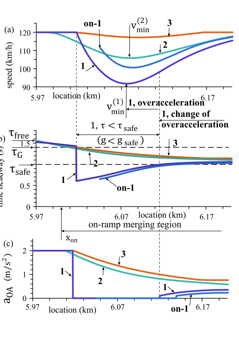
Figure 9: Continuation of Fig. 8(b). (a)–(c) Location-dependencies of microscopic characteristics for some of the vehicles whose numbers are the same as those in Fig. 8(b), respectively: (a) vehicle speeds; (b) vehicle time-headway; (c) overacceleration $a_{\rm OA}$ (4), (6).

First, overacceleration due to safety acceleration of vehicle 1 [$``$1, overacceleration” in Fig. 9(a)] following on-ramp vehicle on-1 occurs. This overacceleration mechanism is the same as explained in Sec. III.3. Later, as can be seen from Figs. 9(b) and 9(c), overacceleration cooperation is realized due to addition overacceleration mechanism $a_{\rm OA}$ (1), (4) [labeled by $``$1, change of overacceleration” in Fig. 9(a)]. For vehicles 2 and 3 following vehicle 1, overacceleration is caused by overacceleration mechanism $a_{\rm OA}$ [Figs. 9(b) and 9(c)] only. In other words, overacceleration cooperation can occur over time [time-sequence of the effects of different overacceleration mechanisms on vehicle 1 and the effect of overacceleration $a_{\rm OA}$ on vehicles 2 and 3 shown in Fig. 9].

Contrary to Fig. 7(a), due to overacceleration cooperation, the speed of vehicle 3 that follows vehicle 2 reaches its maximum value $v_{\rm free}$ already within the local speed decrease at the bottleneck [Fig. 9(a)]. Thus, overacceleration cooperation increases the tendency to free flow. Indeed, in Sec. VII we will show that overacceleration cooperation increases the maintenance of free flow upstream at the bottleneck.

V Effect of overacceleration in road lane on overacceleration through lane-changing

V.1 Prevention of overacceleration through lane-changing due to speed adaptation within the indifferent zone

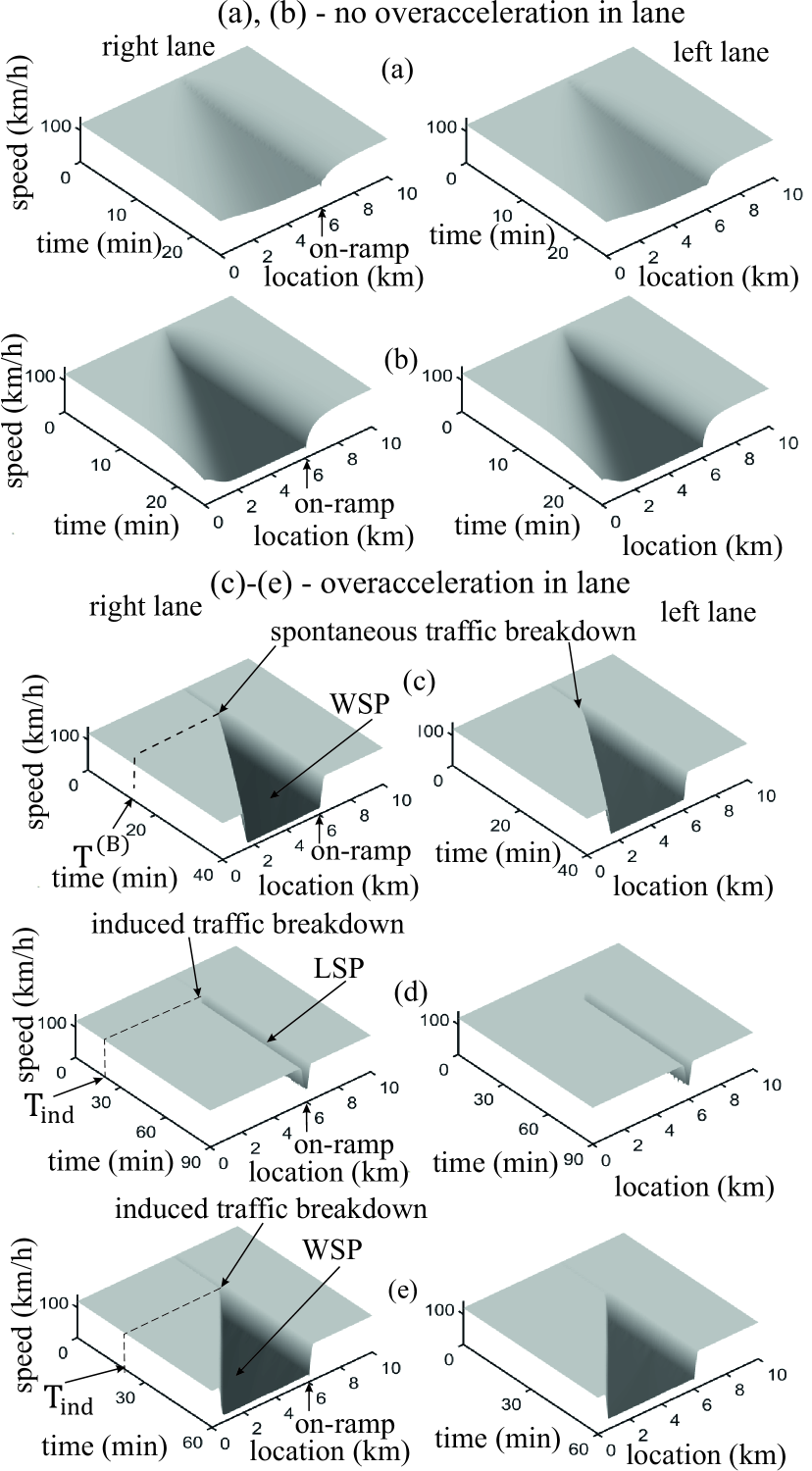
Figure 10: Simulations of the effect of overacceleration in road lane on overacceleration through lane-changing on two-lane road with on-ramp bottleneck at $q_{\rm in}=$ 2000 (vehicles/h)/lane, $\tau_{\rm G}=$ 2 s and different on-ramp inflow rates. Speed in space and time in the right lane (left column) and in the left lane (right column). (a), (b) No overacceleration in road lane – no overacceleration through lane-changing; simulations of model (1)–(15), i.e., at $a_{\rm OA}=$ 0 in (1), (5); (a) $q_{\rm on}=$ 300 vehicles/h, (b) $q_{\rm on}=$ 900 vehicles/h. (c)–(e) Traffic breakdown in model (1)–(14); parameters of overacceleration in road lane: $\alpha_{0}=$ 2 $\rm m/s^{2}$, $\alpha_{1}=$ 0.1 $\rm m/s^{2}$, $k=$ 1. (c) Spontaneous traffic breakdown with WSP formation at $q_{\rm on}=$ 1144 vehicles/h that exceeds slightly the maximum flow rate $q_{\rm on}=q_{\rm on,\ max}=$ 1142 vehicles/h in free flow. (d) LSP induced at bottleneck at the minimum flow rate $q_{\rm on}=q_{\rm on,\ min}=$ 517 vehicles/h at which SP can still be induced in free flow. (e) Induced traffic breakdown at $q_{\rm on}=$ 980 vehicles/h. In (d) and (e), F$\rightarrow$S transition has been induced at $T_{\rm ind}=$ 20 min through addition on-ramp inflow-rate impulse $\Delta q_{\rm on}=$ 1400 vehicles/h of duration $\Delta t=$ 2 min. Parameters of lane-changing: $\tau_{1}=$ 0.5 s, $\tau_{2}=$ 0.3 s, $\delta_{1}=$ 1 m/s, $\delta_{2}=$ 5 m/s. Other parameters are the same as those in Fig. 2. WSP is widening SP, LSP is localized SP, SP is synchronized flow pattern.

First, we consider traffic breakdown on two-lane road under assumption $\alpha=$ 0 (15). Then, contrary to Helly’s model for motion of automated-driving vehicles used in Kerner2023C , in model (1)–(15) we find that no overacceleration through lane-changing is realized [Figs. 10(a) and 10(b)]. This result is explained as follows. As shown in Sec. III.1 for single-lane road (Fig. 2), vehicle 1 following on-ramp vehicle on-1 should decelerate strongly resulting in deceleration of following vehicles [vehicles 2 and 3 in Fig. 3(a)] due to speed adaptation (16). The same effect we observe on two-lane road: In the right lane, a wave of a speed decrease propagating upstream occurs [Figs. 10(a) and 10(b)].

The speed adaptation effect (16) is also realized for vehicles in the left lane that follow a slower moving vehicle that has just changed from the right lane to the left lane. For this reason, in the left lane we also observe a wave of the speed decrease propagating upstream [Figs. 10(a) and 10(b)]. Under used parameters in model (1)–(15), i.e., when no overacceleration exists in road lane, there is also no overacceleration through lane-changing and, respectively, traffic breakdown does not exhibit the nucleation character. This result can be explained as follows: Speed adaptation within the indifferent zone for car-following (16) is stronger than vehicle acceleration to free flow downstream and, therefore, the acceleration cannot maintain free flow upstream of the bottleneck.

V.2 Microscopic features of overacceleration on two-lane road

If assumption $\alpha=$ 0 (15) is not applied, then contrary to Figs. 10(a) and 10(b), due to the existence of overacceleration in road lane $a_{\rm OA}$ (4) traffic on two-lane road becomes metastable with respect to an F$\rightarrow$S transition [Figs. 10(c)–10(e)]. There is the following common feature of vehicle overacceleration found in Kerner2023C for automated-driving vehicles moving based on Helly’s model and in model (1)–(14): When free flow [Figs. 11(a) and 11(b)] transforms into synchronized flow [Figs. 11(c) and 11(d)], there is a discontinuity in the rate of R$\rightarrow$L lane-changing denoted by $R_{\rm RL}$ (Fig. 12). This causes the discontinuity in the acceleration rate $R_{\rm OA}$ in accordance with equation $R_{\rm OA}=R_{\rm RL}$ (Fig. 12). There are the following differences in features of overacceleration in Helly’s model for automated-driving vehicles Kerner2023C and model (1)–(14) [Figs. 13–15]:

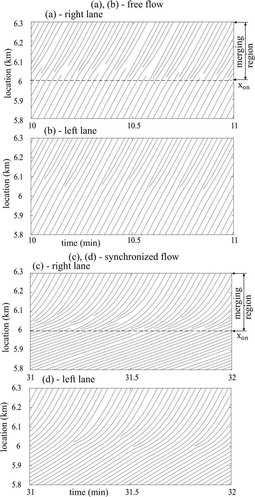
Figure 11: Continuation of Fig. 10(e). (a), (b) Some of simulated vehicle trajectories within local speed decrease in free flow at bottleneck at time $t<T_{\rm ind}=$ 20 min in the right (a) and left (b) lanes. (c), (d) Some of simulated vehicle trajectories within synchronized flow at bottleneck at time $t>T_{\rm ind}+\Delta t$.

(i) When due to lane-changing of vehicle 2 (Fig. 13) space gap $g$ between vehicle 1 and 3 becomes larger than synchronization gap $G$ [i.e., $\tau>\tau_{\rm G}$ in Fig. 14(b)], acceleration of vehicle 3 given by Eq. (5) increases considerably due to overacceleration in road lane $a_{\rm OA}$ (4), (6) [Fig. 14(c)]. As a result, in model (1)–(14) vehicle 3 accelerates strongly while reaching the maximum speed $v_{\rm free}$ quickly [Fig. 14(a)] .

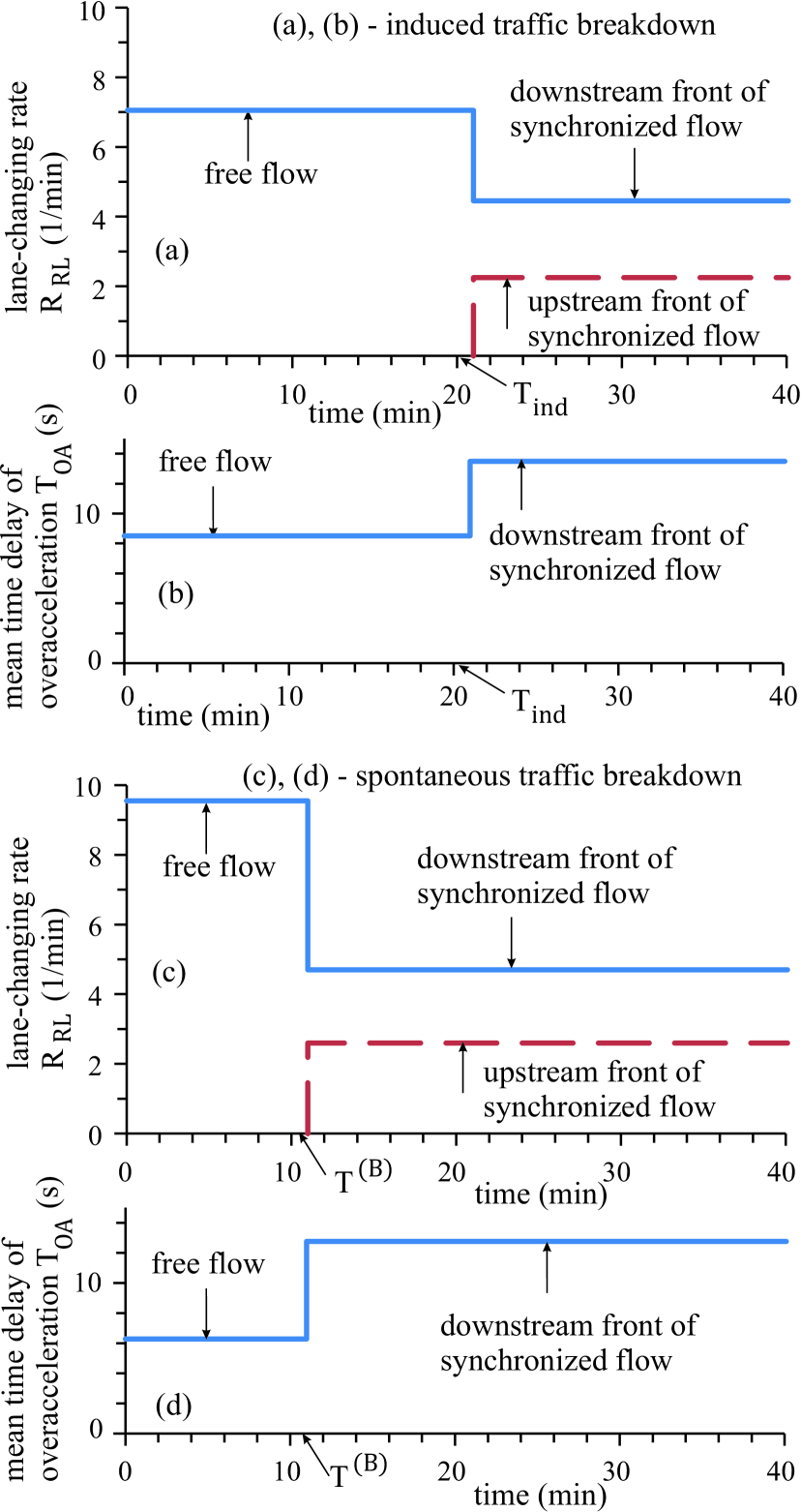
Figure 12: Continuation of Figs. 10(c) and 10(e). Time-dependencies of the lane-changing rate $R_{\rm RL}$ (a), (c) and the mean time delay in overacceleration $T_{\rm OA}=1/R_{\rm OA}$ (b), (d). Solid blue colored curves are related to cases in which $R_{\rm OA}=R_{\rm RL}$, where $R_{\rm OA}$ is the overacceleration rate. In (a), (c), dashed red colored curves are time-dependencies of the lane-changing rate $R^{\rm(up)}_{\rm RL}$ at the upstream front of synchronized flow. (a), (b) For induced traffic breakdown shown in Fig. 10(e). (c), (d) For spontaneous traffic breakdown shown in Fig. 10(c). Values $R_{\rm OA}$, $R^{\rm(up)}_{\rm RL}$, and $T_{\rm OA}$ have been averaged in free flow (during time intervals $0\leq t<T_{\rm ind}$, $T_{\rm ind}=$ 20 min and $0\leq t<T^{\rm(B)}$, $T^{\rm(B)}\approx$ 10.8 min for induced and spontaneous breakdowns, respectively) and in synchronized flow (during time intervals $T_{\rm ind}+\Delta t<t\leq 40$ min and $T^{\rm(B)}<t\leq 40$ min for induced and spontaneous breakdowns, respectively).

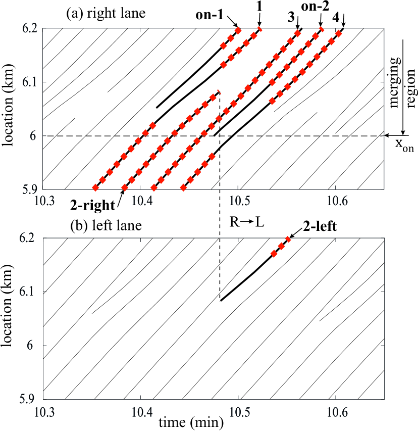
Figure 13: Continuation of Fig. 10(e). (a), (b) Simulated vehicle trajectories within local speed decrease in free flow at bottleneck in the right lane (a) and left lane (b) at time $t<T_{\rm ind}=$ 20 min. R$\rightarrow$L lane-changing of vehicle 2 is marked by dashed vertical lines R$\rightarrow$L. Part of trajectories within which condition $a_{\rm OA}>0$ is satisfied are marked through colored red squares.

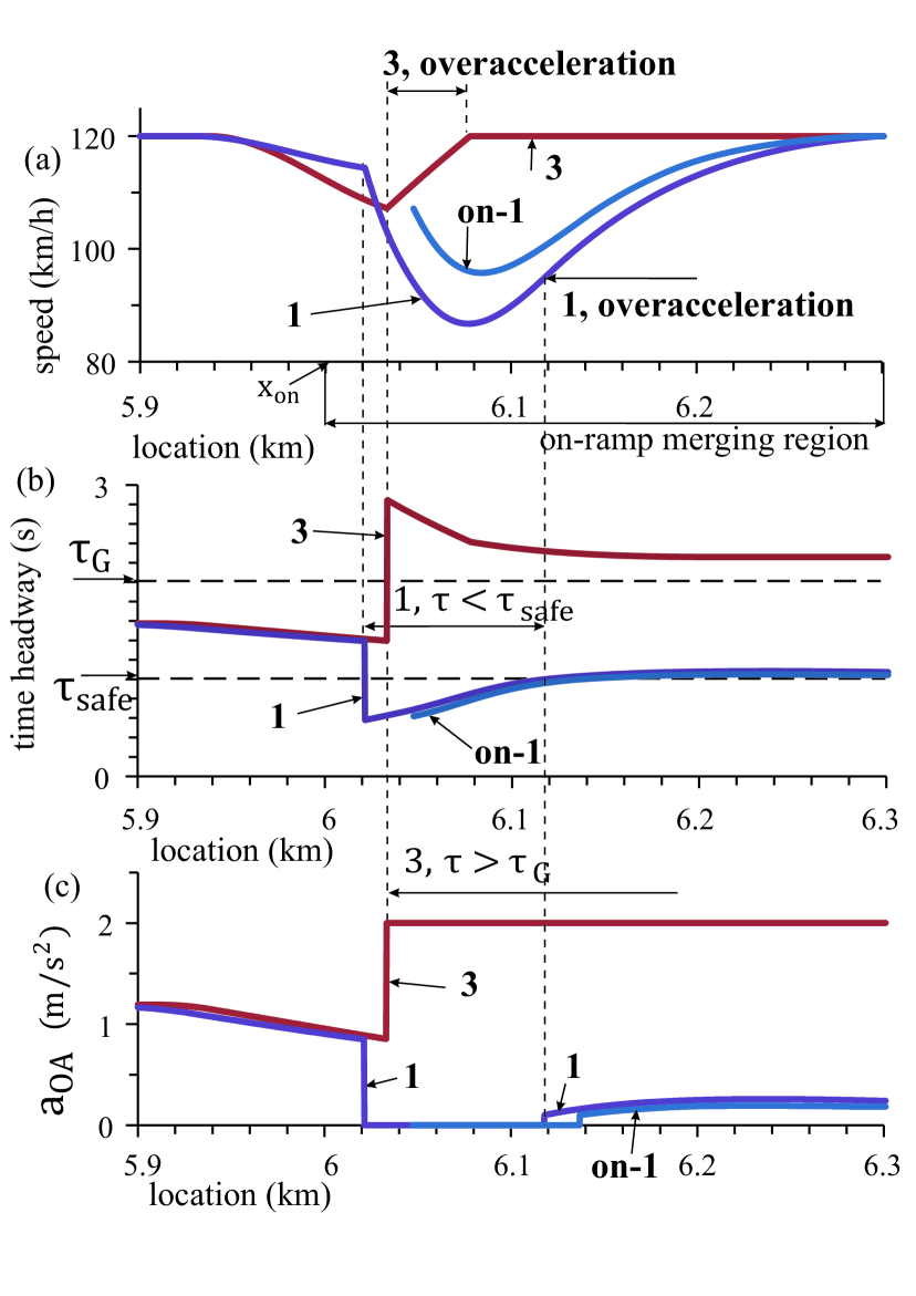
Figure 14: Continuation of Fig. 13. (a)–(c) Location-dependencies of microscopic characteristics for some of the vehicles whose numbers are the same as those in Fig. 13, respectively: (a) vehicle speeds; (b) vehicle time-headway; (c) overacceleration $a_{\rm OA}$ (4), (6).

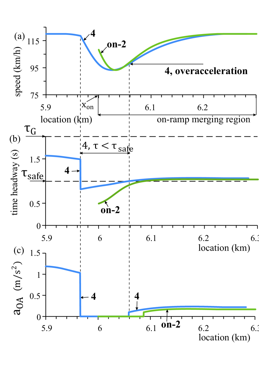
Figure 15: Continuation of Fig. 13. (a)–(c) Location-dependencies of microscopic characteristics for some of the vehicles whose numbers are the same as those in Fig. 13, respectively: (a) vehicle speeds; (b) vehicle time-headway; (c) overacceleration $a_{\rm OA}$ (4), (6).

(ii) There can be overacceleration mechanism(s) in road lane that maintains (in addition to lane-changing) free flow at the bottleneck: After time-headway of vehicle 4 in Fig. 13 following the on-ramp vehicle on-2 satisfies condition $\tau\geq\tau_{\rm safe}$, vehicle acceleration increases through the term $a_{\rm OA}$ [Figs. 15(b) and 15(c)]. Overacceleration of vehicle 4 leads to recovering of free flow already within on-ramp merging region [$``$4, overacceleration” in Fig. 15(a)].

V.3 Effect of safety acceleration on overacceleration on two-lane road

The situation considered in Figs. 10(a) and 10(b) changes basically if we decrease the synchronization time-headway from $\tau_{\rm G}=$ 2 s to shorter value $\tau_{\rm G}=$ 1.4 s that satisfies condition (18). As we know from Sec. III.3, in this case there is overacceleration in road lane through safety acceleration. Then, traffic breakdown does exhibit the nucleation character (Fig. 16). We have found (not shown) that, as in the case shown in Fig. 12, a discontinuous character of the overacceleration rate $R_{\rm OA}$ is realized, i.e., there is also overacceleration through lane-changing.

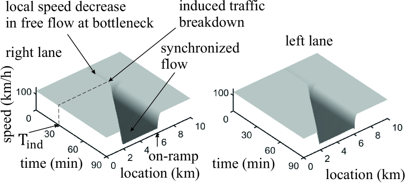
Figure 16: Effect of overacceleration through safety acceleration in road lane at $\tau_{\rm G}=$ 1.4 s on overacceleration through lane-changing on two-lane road with bottleneck; simulations of model (1)–(15), i.e., at $a_{\rm OA}=$ 0 in (1), (5). $q_{\rm on}=$ 700 vehicles/h. F$\rightarrow$S transition has been induced at $T_{\rm ind}=$ 30 min through addition on-ramp inflow-rate impulse $\Delta q_{\rm on}=$ 900 vehicles/h of duration $\Delta t=$ 2 min. Other model parameters are the same as those in Figs. 10(a) and 10(b).

VI Critical nucleus for spontaneous traffic breakdown

As for Helly’s model used for automated-driving vehicles in Kerner2023B , in model of Sec. II at a given $q_{\rm in}$ when the on-ramp inflow rate $q_{\rm on}$ increases, then at some $q_{\rm on}>q_{\rm on,\ max}$ the minimum speed within a local speed decrease at the bottleneck decreases over time and after a time-delay $T^{\rm(B)}$ spontaneous traffic breakdown (spontaneous F$\rightarrow$S transition) occurs [Figs. 10(c) and 17(a)]. Here we reveal microscopic features of the critical nucleus for spontaneous traffic breakdown.

VI.1 Microscopic characteristics of critical nucleus

On single-lane road [Figs. 17 and 18] and on two-lane road [Figs. 19 and 20], during interval $0<t<T^{\rm(B)}$ a minimum speed $v_{\rm min}$ within the local speed decrease at the bottleneck is a decreasing time-function [minimum speeds of vehicles 1–3 in Fig. 18(a) for single-lane road and minimum speeds of vehicles 1–3 and 7–9 in Fig. 20 for two-lane road]. When $v_{\rm min}$ becomes less than $v_{\rm syn}$ (4), a state within the local speed decrease can be considered synchronized flow. Thus, free flow persists upstream of the bottleneck, while synchronized flow is only within the local speed decrease at the bottleneck.

We have found that time-delay of spontaneous traffic breakdown $T^{\rm(B)}$ is determined by a saturation in decrease of $v_{\rm min}$: At $t>T^{\rm(B)}$ without further noticeable decrease in $v_{\rm min}$, the upstream front of synchronized flow moves upstream of the bottleneck, i.e., free flow upstream of the bottleneck transforms over time into synchronized flow propagating upstream [vehicles 4–6 in Fig. 18 and vehicles 4–6 and 10–12 in Fig. 20]. The beginning of the upstream propagation of synchronized flow can be seen from a comparison of microscopic speeds along trajectories 4 and 8 in Fig. 18(b) for single-lane road as well as a comparison of microscopic speeds along trajectories 16 and 20 for two-lane road in Fig. 20(c).

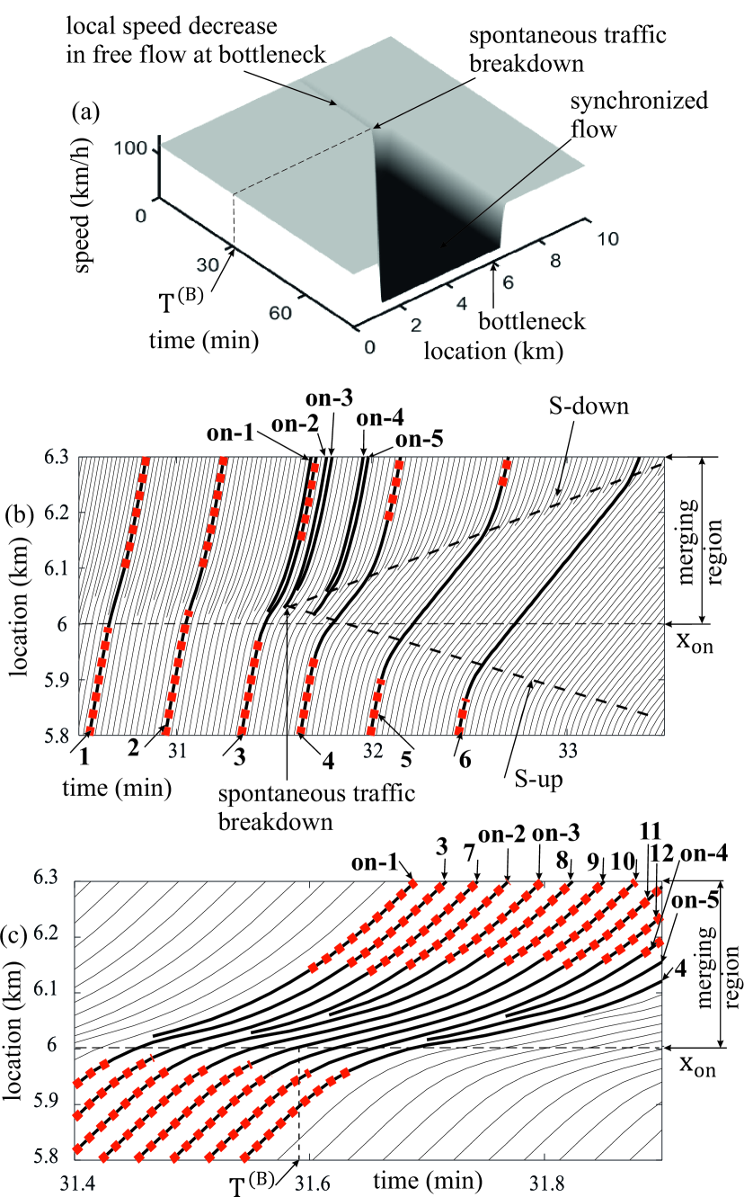
Figure 17: Spontaneous traffic breakdown on single-lane road with on-ramp bottleneck. Simulations of the same model (1)–(10), (14) at $\tau_{\rm G}=$ 1.4 s, $q_{\rm in}=$ 2000 vehicles/h as that used in Fig. 8, however, at $q_{\rm on}=$ 809 vehicles/h that is only slightly higher than $q_{\rm on}=q_{\rm on,\ max}=$ 807 vehicles/h. Other model parameters are the same as those in Fig. 8. (a), (b) Speed in space and time: Local speed decrease at bottleneck in free flow (a) and synchronized flow pattern (SP) (b) that occurs spontaneously in free flow after time-delay $T^{\rm(B)}\approx$ 31.6 min. (c) Some of simulated vehicle trajectories within local speed decrease in free flow at bottleneck in a vicinity of time $t=T^{\rm(B)}$; part of trajectories within which condition $a_{\rm OA}>0$ is satisfied are marked through colored red squares.

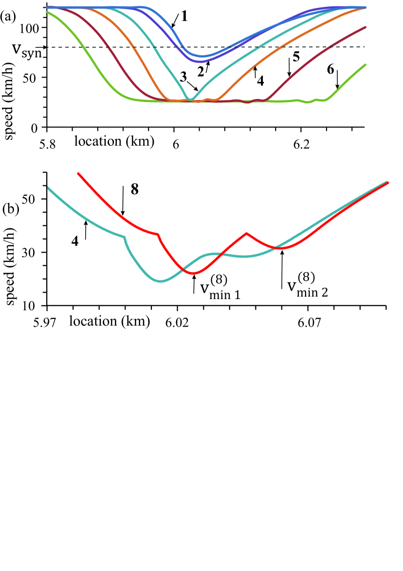
Figure 18: Location-dependence of vehicle speeds those trajectories are shown by the same vehicle numbers in Figs. 17(b) and 17(c): (a) Averaged speed along trajectories (1-sec averaged data) shown in Fig. 17(b); dashed line $v=v_{\rm syn}$ separates road regions on vehicle trajectories within which overacceleration $a_{\rm OA}$ is either more than zero (on and above the line) or it is equal to zero (below the line). (b) Microscopic (not averaged data) speeds along trajectories 4 and 8 shown in Figs. 17(b) and 17(c).

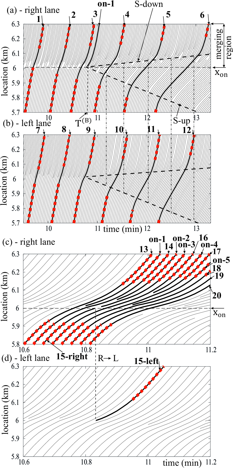
Figure 19: Continuation of Fig. 10(c). (a), (b) Simulated vehicle trajectories within local speed decrease in free flow on two-lane road with bottleneck showing spontaneous traffic breakdown occurring after time-delay at $T^{\rm(B)}\approx$ 10.8 min. (c), (d) Some of simulated vehicle trajectories of (a), (b) shown in a shorter time-scale; parts of trajectories upstream of the bottleneck within which condition $a_{\rm OA}>0$ is satisfied are marked through colored red squares.

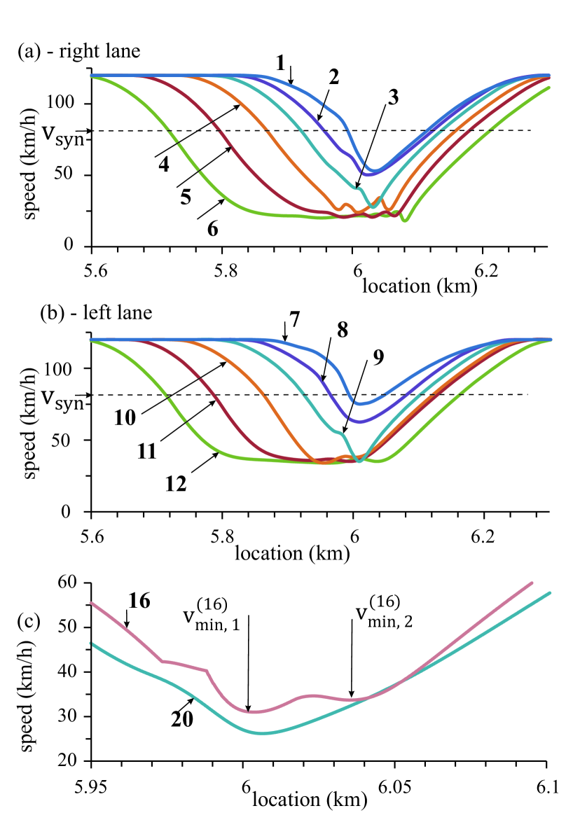
Figure 20: Continuation of Figs. 19(a)–19(c). (a), (b) Location-dependence of averaged vehicle speeds (1-sec averaged data); dashed lines $v=v_{\rm syn}$ separate road regions on vehicle trajectories within which overacceleration $a_{\rm OA}$ is either more than zero (on and above the lines) or it is equal to zero (below the lines). (c) Location-dependence of speeds (not averaged data) of vehicles 16 and 20. Trajectories are shown with the same vehicle numbers as those in Figs. 19(a)– 19(c), respectively.

Thus, the critical nucleus at the bottleneck is a local speed decrease at the bottleneck caused by the last on-ramp vehicle or the last sequence on-ramp vehicles merging from the on-ramp at $t<T^{\rm(B)}$ at which the speed decrease is still localized at the bottleneck. This means that the next on-ramp vehicle or sequence of on-ramp vehicles that have merged from the on-ramp at $t=T^{\rm(B)}$ cause another local speed decrease that cannot be localized at the bottleneck any more: At $t>T^{\rm(B)}$ the irreversible upstream propagation of synchronized flow occurs.

There can be one, two, or more minimums of the synchronized flow speed within the nucleus. In Fig. 17(c), two following each other on-ramp vehicles have merged onto the main road (vehicles on-2 and on-3). This results in two speed minimums for vehicle 8 ($v^{\rm(8)}_{\rm min,\ 1}$ and $v^{\rm(8)}_{\rm min,\ 2}$ in Fig. 18(b)) that follows vehicles on-2 and on-3. A similar result is realized on two-lane road for vehicle 16 following two on-ramp vehicles (vehicles on-2 and on-3 in Fig. 19(c)). This leads to two speed minimums for vehicle 16 ($v^{\rm(16)}_{\rm min,\ 1}$ and $v^{\rm(16)}_{\rm min,\ 2}$ in Fig. 20(c)). The lowest speed minimum within the critical nucleus can be considered a microscopic critical speed for traffic breakdown (F$\rightarrow$S transition).

VI.2 Effect of overacceleration in road lane $a_{\rm OA}$ on critical nucleus development

When time $t$ is not very close to $T^{\rm(B)}$, the minimum speed $v_{\rm min}$ within the local speed decrease at the bottleneck is not considerably less than $v_{\rm syn}$ [e.g., $v^{(1)}_{\rm min}\approx$ 72.2 km/h for vehicles 1 on single-lane road in Fig. 18(a) and $v^{(1)}_{\rm min}\approx$ 53.3 km/h for vehicles 1 on two-lane road in Fig. 20(a)]. As a result, upstream of the bottleneck overacceleration $a_{\rm OA}>0$ with the exception of a narrow road region at the bottleneck within which $v<v_{\rm syn}$ [Figs. 18(a), 20(a) and 20(b)] and, therefore, $a_{\rm OA}=0$.

When $t\rightarrow T^{\rm(B)}$, then the effect of overacceleration $a_{\rm OA}$ on the maintenance of free flow at the bottleneck becomes weaker. Indeed, due to a decrease in $v_{\rm min}$, the size of a road region in the bottleneck vicinity within which the speed $v<v_{\rm syn}$, i.e., overacceleration $a_{\rm OA}=$ 0, increases [this can be seen on trajectories 1–3 for single-lane road in Fig. 18(a) and on trajectories 1–3 and 7–9 for two-lane road in Figs. 20(a),(b)]. Thus, at $t\rightarrow T^{\rm(B)}$ the effect of overacceleration $a_{\rm OA}$ on the critical nucleus development is caused by the increase in the road region size in the bottleneck vicinity within which $a_{\rm OA}=$ 0.

VII A proof of effect of overacceleration on vehicular traffic

• The main effect of overacceleration on vehicular traffic at a bottleneck is the maintenance of free flow upstream of the bottleneck, i.e., the prevention of traffic breakdown (F$\rightarrow$S transition).

To provide a proof of this statement, we show than for the same chosen flow rate in free flow $q_{\rm in}$ upstream of the bottleneck, the stronger the effect of overacceleration on vehicular traffic, the larger the maximum on-ramp inflow rate $q_{\rm on}=q_{\rm on,\ max}$ at which free flow upstream of the bottleneck is still maintained. Through the revealing of different overacceleration mechanisms as well as their cooperation (Secs. IV and V.2), such a proof is possible to do as explained below with the use of Fig. 21 for single-lane road and Fig. 22 for two-lane road.

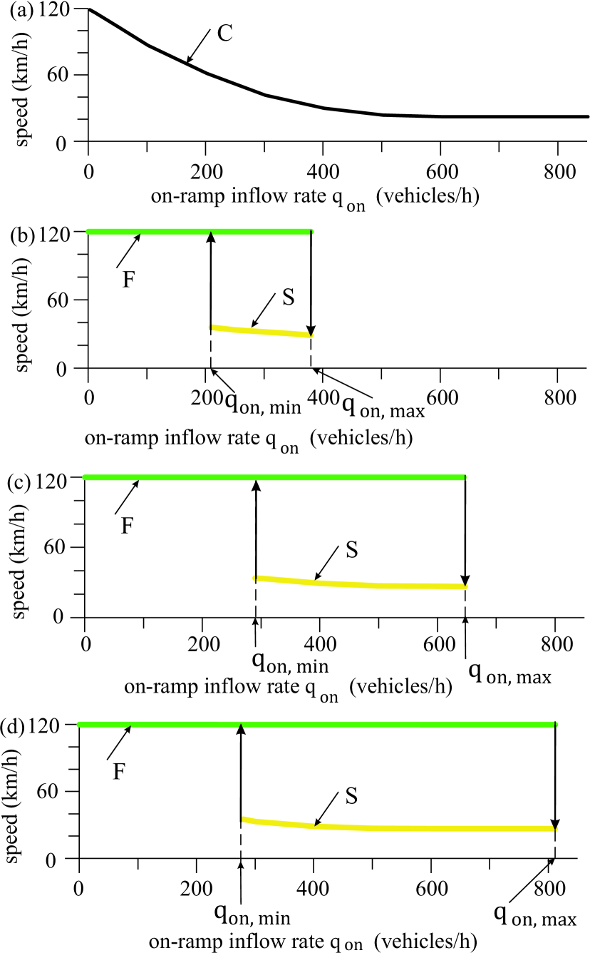
Figure 21: Proof of effect of overacceleration on vehicular traffic on single-lane road with the use of speed–on-ramp-inflow characteristics calculated at $q_{\rm in}=$ 2000 vehicles/h: (a) No overacceleration, model and parameters of Fig. 2. (b) Overacceleration mechanism through safety acceleration only, model and parameters of Fig. 6. (c) Overacceleration due to $a_{\rm OA}$ (4), (6) in model (1)–(10), (14) with parameters: $\alpha_{0}=$ 2 $\rm m/s^{2}$, $\alpha_{1}=$ 0.1 $\rm m/s^{2}$, $k=$ 1; other model parameters are the same as those in Fig. 2. (d) Cooperation of overacceleration mechanisms through safety acceleration at $g_{\rm free}>G$ (18) and due to overacceleration mechanism $a_{\rm OA}$ (4), (6); model and parameters of Fig. 8. Contrary to (d), in (c) there is only overacceleration mechanism $a_{\rm OA}$; this is because due to $\tau_{\rm G}=$ 2 s used in (c) condition (18) is not satisfied and, therefore, safety acceleration cannot be considered overacceleration at the given $q_{\rm in}$. C – congested traffic, F – free flow, S – synchronized flow. $q_{\rm on}=q_{\rm on,\ min}$ is a minimum on-ramp flow rate related to a minimum highway capacity $C_{\rm min}=q_{\rm in}+q_{\rm on,\ min}$, whereas $q_{\rm on}=q_{\rm on,\ max}$ is related to a maximum highway capacity $C_{\rm max}=q_{\rm in}+q_{\rm on,\ max}$. Within the range $q_{\rm on,\ min}\leq q_{\rm on}<q_{\rm on,\ max}$ either free flow or an SP can exist at the bottleneck; at $q_{\rm on}<q_{\rm on,\ min}$ no congested patterns can be induced in free flow, whereas at $q_{\rm on}>q_{\rm on,\ max}$ the SP occurs spontaneously at the bottleneck after a time delay $T^{\rm(B)}$. Calculated parameters: $(q_{\rm on,\ min},\ q_{\rm on,\ max})=$ (217, 372) vehicles/h (b), (293, 648) vehicles/h (c), (280, 807) vehicles/h (d).

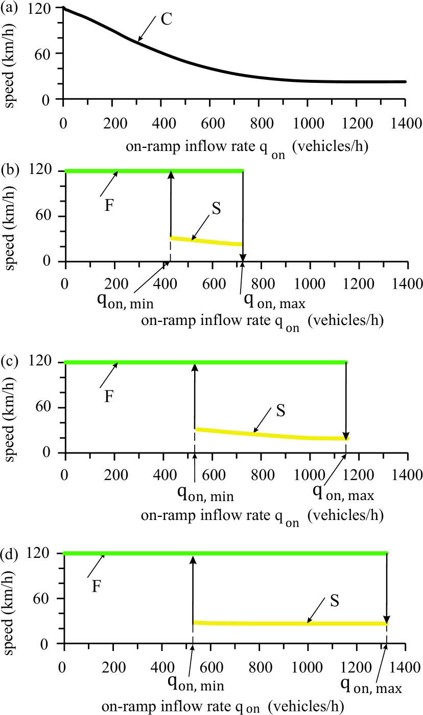
Figure 22: Proof of effect of overacceleration on vehicular traffic on two-lane road with the use of speed–on-ramp-inflow characteristics calculated at $q_{\rm in}=$ 2000 (vehicles/h)/lane: (a) No overacceleration, model and parameters of Figs. 10(a) and 10(b). (b) Model and parameters of Fig. 16. (c) Model and parameters of Figs. 10(c)–10(e). (d) Model (1)–(14) at $\tau_{\rm G}=$ 1.4 s; other parameters are the same as those in Figs. 10(c)–10(e). C – congested traffic, F – free flow, S – synchronized flow. Minimum and maximum highway capacities, respectively, are: $C_{\rm min}=2q_{\rm in}+q_{\rm on,\ min}$ and $C_{\rm max}=2q_{\rm in}+q_{\rm on,\ max}$. Calculated parameters: $(q_{\rm on,\ min},\ q_{\rm on,\ max})=$ (430, 721) vehicles/h (b), (517, 1142) vehicles/h (c), (525, 1324) vehicles/h (d).

In Figs. 21(a) and 22(a), there is no overacceleration (Secs. III.1 and V.1). Then, vehicles on the main road moving initially at free flow speed $v_{\rm free}$ upstream of the bottleneck must decelerate due to vehicles merging from the on-ramp. Through this speed adaptation effect (16), at the given $q_{\rm in}$ the larger the on-ramp inflow-rate $q_{\rm on}$, the lower the average vehicle speed upstream of the bottleneck. This means that speed adaptation is the cause for the emergence of congested traffic at the bottleneck.

Overacceleration is the opposite effect to speed adaptation. Indeed, contrary to Figs. 21(a) and 22(a), in Figs. 21(b)–21(d) and 22(b)–22(d) when overacceleration is realized at the bottleneck, free flow can be self-maintained upstream of the bottleneck up to some maximum on-ramp inflow rate $q_{\rm on}=q_{\rm on,\ max}$, i.e., up to the maximum highway capacity $C_{\rm max}=q_{\rm in}+q_{\rm on,\ max}$. Thus, as long as $q_{\rm on}<q_{\rm on,\ max}$ (i.e., highway capacity is less than $C_{\rm max}$) overacceleration occurring in Figs. 21(b)–21(d) and 22(b)–22(d) prevents traffic congestion at the bottleneck caused by speed adaptation in Figs. 21(a) and 22(a).

On single-lane road, when overacceleration is caused by safety acceleration at $g_{\rm free}>G$ (18) only (Sec. III.3), then the maximum on-ramp inflow-rate $q_{\rm on,\ max}$ and, therefore, the maximum capacity $C_{\rm max}$ [Fig. 21(b)] are, respectively, less than these values are when overacceleration is caused by the term $a_{\rm OA}$ (4) [Fig. 21(c)]. This means that at model parameters under consideration the effect of overacceleration $a_{\rm OA}$ (4) on the maintenance of free flow at the bottleneck is stronger than the overacceleration effect due to safety acceleration. The stronger the overacceleration effect on free flow is, the larger the on-ramp inflow rate $q_{\rm on,\ max}$ at which free flow is still self-maintained at the bottleneck. This statement is confirmed by the result that the greatest values $q_{\rm on,\ max}$ and $C_{\rm max}$ are realized when overacceleration is further increased through cooperation of overacceleration $a_{\rm OA}$ (4) and overacceleration caused by safety acceleration at $g_{\rm free}>G$ (18) [Fig. 21(d)].

As on single-lane road, the stronger the overacceleration effect on free flow on two-lane road is, the larger the on-ramp inflow rate $q_{\rm on,\ max}$ at which free flow is still self-maintained at the bottleneck. Indeed, in Fig. 22(b) overacceleration in road lane is determined by safety acceleration at $g_{\rm free}>G$ (18) only; as explained above [Fig. 21(b)], this overacceleration mechanism is weaker than that determined by overacceleration $a_{\rm OA}$ (4). Therefore, we have found that cooperation of overacceleration due to safety acceleration at $g_{\rm free}>G$ (18) and overacceleration through lane-changing can self-maintain free flow at the bottleneck only up to a relative small on-ramp inflow rate $q_{\rm on,\ max}$ [Fig. 22(b)]. In Fig. 22(c), overacceleration in road lane is determined by $a_{\rm OA}$ (4) that, as above-mentioned, is stronger than overacceleration due to safety acceleration at $g_{\rm free}>G$ (18). As a result, we have found that cooperation of two overacceleration mechanisms caused by $a_{\rm OA}$ and through lane-changing maintains free flow at the bottleneck up to a considerably larger value $q_{\rm on,\ max}$ [Fig. 22(c)] than that in Fig. 22(b).

Finally, in Fig. 22(d) related to model (1)–(14) at $\tau_{\rm G}=$ 1.4 s there is cooperation of three mechanisms of overacceleration (due to $a_{\rm OA}$ (4), through safety acceleration at $g_{\rm free}>G$ (18), and through lane-changing). Then, we have found the greatest maximum on-ramp inflow-rate $q_{\rm on,\ max}$ (and, therefore, the greatest maximum highway capacity $C_{\rm max}$ at the given $q_{\rm in}$). This shows that the cooperation of three mechanisms of overacceleration exhibits the strongest effect on the self-maintaining of free flow at the bottleneck.

VIII Microscopic effect of overacceleration cooperation on S$\rightarrow$F instability

VIII.1 Overacceleration cooperation and S$\rightarrow$F instability on two-lane road without bottlenecks

In Kerner2023C , we have shown that overacceleration $a_{\rm OA}$ (4) on single-lane road without bottlenecks can cause an S$\rightarrow$F instability that exhibits the nucleation nature. It can be expected that on two-lane road overacceleration $a_{\rm OA}$ (4) can also cause the S$\rightarrow$F instability (Fig. 23). Indeed, a local disturbance in initial homogeneous synchronized flow caused by an addition acceleration of one of the vehicles during $\delta t=$ 5 s initiates the S$\rightarrow$F instability [Figs. 23(a) and 23(b)]. Contrarily, if the same vehicle accelerates during $\delta t=$ 4.5 s (i.e., only 0.5 s shorter), then no S$\rightarrow$F instability occurs [Fig. 23(c)]. Here we show that cooperation of overacceleration in road lane $a_{\rm OA}$ (4) and overacceleration caused by lane-changing (Sec. V.2) leads to spatiotemporal lane-changing effects that qualitatively change the dynamics of the S$\rightarrow$F instability in comparison with that found in Kerner2023C .

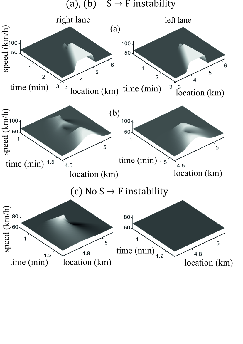
Figure 23: Nucleation nature of S$\rightarrow$F instability on two-lane road caused by cooperation of overacceleration in road lane and due to lane-changing. Simulations with model (1)–(14) at $\tau_{\rm G}=$ 1.4 s made on two-lane road of length 8 km without bottlenecks with initial steady synchronized flow state at speed $v=$ 70 km/h and space gap between vehicles $g=$ 33 m. Vehicle speed is space and time in the right lane (left subplots) and in left lane (right subplots): (a) S$\rightarrow$F instability is caused by initial local speed increase of a vehicle [vehicle 1 in Fig. 24(a)] moving in the right lane simulated through short-time acceleration of the vehicle with $a=$ 1 $\rm m/s^{2}$ during $\delta t=$ 5 s. (b) The beginning of the S$\rightarrow$F instability in (a) shown in a larger scale. (c) S$\rightarrow$F instability does not occur if the same vehicle as that in (a), (b) accelerates with the same acceleration, however, during $\delta t=$ 4.5 s, i.e., 0.5 s shorter. Other model parameters are the same as those in Figs. 10(c)–10(e).

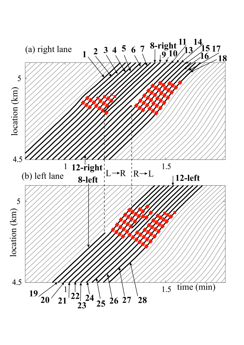
Figure 24: Continuation of Figs. 23(a) and 23(b). (a), (b) Simulated vehicle trajectories within local speed increase in synchronized flow in the right lane (a) and left lane (b). L$\rightarrow$R lane-changing of vehicle 8 is marked by dashed vertical line L$\rightarrow$R. R$\rightarrow$L lane-changing of vehicle 12 is marked by dashed vertical line R$\rightarrow$L. Part of trajectories within which condition $a_{\rm OA}>0$ is satisfied are marked through colored red squares.

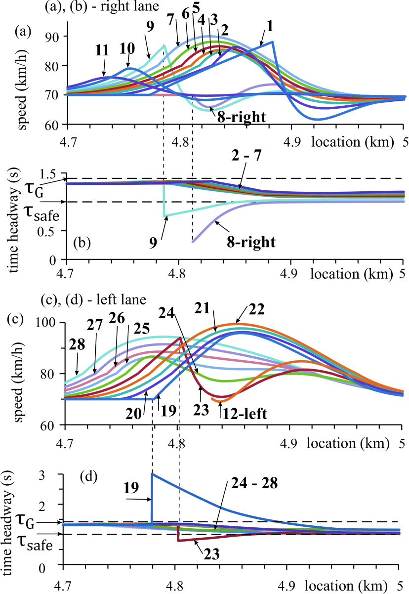
Figure 25: Continuation of Fig. 24. Microscopic vehicle speeds (a), (c) and time headway (b), (d) for right lane (a), (b) and left lane (c), (d) for some of the vehicles whose trajectories are labeled by the same numbers as those in Fig. 24, respectively.

Acceleration of vehicle 1 [Figs. 24(a) and 25(a)] causes a continuous increase in the speed of following vehicles 2–7 in the right lane [Fig. 25(a)]. As in Kerner2023C , this S$\rightarrow$F instability causing the avalanche-like local speed increase in the initial synchronized flow is due to overacceleration $a_{\rm OA}$ (4) in the right lane: Indeed, regions on trajectories, in which condition $a_{\rm OA}>0$ is satisfied, become broader along the successive sequence of vehicles 2–7 [Fig. 24(a)].

VIII.1.1 Interruption of S$\rightarrow$F instability

However, contrary to single-lane road studied in Kerner2023C , vehicles in the left lane that move initially in synchronized flow at $v=$ 70 km/h search for the opportunity to change to the higher speed region caused by the S$\rightarrow$F instability in the right lane. After vehicle 8 in the left lane [vehicle 8-left in Fig. 24(b)] has changed to the right lane [vehicle 8-right in Figs. 24(a) and 25(a)], the situation changes basically: Vehicles 9–11 in the right lane that follow vehicle 8-right begin to decelerate [Fig. 25(a)]. Because the speeds of vehicles 10 and 11 become less than $v_{\rm syn}=$ 80 km/h in (4), along trajectories of vehicle 10 and 11 overacceleration $a_{\rm OA}=$ 0 [Fig. 24(a)]. This means that the S$\rightarrow$F instability in the right lane is abrupt interrupted through L$\rightarrow$R lane-changing. The interruption of the development of the S$\rightarrow$F instability in the right lane occurs because just after lane-changing the speed of vehicle 8-right is considerably lower than the speed of vehicle 9 whereas time headway of vehicle 9 to preceding vehicle 8-right is considerably shorter than the safe time-headway $\tau_{\rm safe}$; therefore, vehicle 9 must decelerate strongly [Figs. 25(a) and 25(b)].

VIII.1.2 S$\rightarrow$F instability in left lane causing repetition of S$\rightarrow$F instability in right lane

There are three dynamic effects following L$\rightarrow$R lane-changing: (i) The interruption of the S$\rightarrow$F instability in the right lane (Sec. VIII.1.1), (ii) the beginning of the S$\rightarrow$F instability in the left lane, and (iii) the repetition of the S$\rightarrow$F instability in the right lane.

The S$\rightarrow$F instability in the left lane is caused by overacceleration through L$\rightarrow$R lane-changing of vehicle 8: Time headway of vehicle 19 in the left lane increases considerably [Figs. 24(b), 25(c) and 25(d)]. This results in overacceleration of vehicle 19 [$a_{\rm OA}>$ 0 on trajectory 19 in Fig. 24(b)]. This overacceleration causes the S$\rightarrow$F instability in the left lane [vehicles 20–22 in Fig. 24(b)].

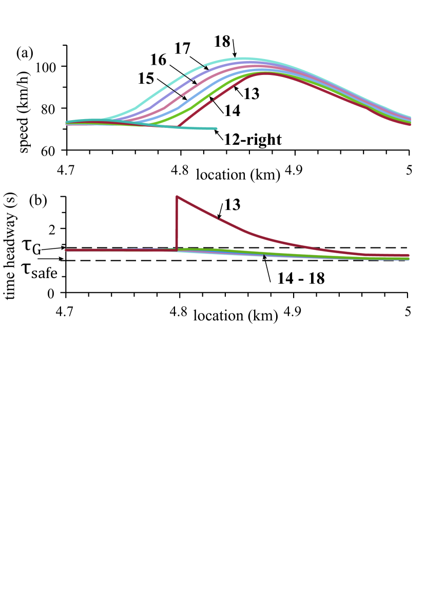
Figure 26: Continuation of Fig. 24. Repetition of S$\rightarrow$F instability in right lane. Microscopic vehicle speeds (a) and time headway (b) for right lane for some of the vehicles whose trajectories are labeled by the same numbers as those in Fig. 24, respectively.

Now vehicles following vehicle 8-right in the right lane, which due to the interruption of the S$\rightarrow$F instability in the right lane should move in synchronized flow, search for the opportunity to change to a higher speed region caused by the S$\rightarrow$F instability in the left lane: After vehicle 12 in the right lane [vehicle 12-right in Fig. 24(a)] has changed to the left lane [vehicle 12-left in Figs. 24(b) and 25(c))], two effects occur: (i) Because vehicle 12-right changes the lane, time headway of vehicle 13 in the right lane increases considerably [Fig. 26(b)]. (ii) Vehicle 23 that follows vehicle 12-left in the left lane decelerates strongly [Fig. 25(c)].

The first effect of R$\rightarrow$L lane-changing causes repetition of the S$\rightarrow$F instability in the right lane (Fig. 26). Indeed, time headway of vehicle 13 increases; this leads to overacceleration of vehicle 13 [$a_{\rm OA}>$ 0 on trajectory 13 in Fig. 24(a)]. This causes the S$\rightarrow$F instability in the right lane [vehicles 14–18 in Fig. 26(a)].

The second effect of R$\rightarrow$L lane-changing, which leads to deceleration of vehicle 23 following vehicle 12-left, does not cause interruption of the S$\rightarrow$F instability in the left lane. This is in contrast to L$\rightarrow$R lane-changing of vehicle 8 causing the interruption of the S$\rightarrow$F instability in the right lane (Sec. VIII.1.1). To explain it, we note that along trajectory of vehicle 24 following vehicle 23 in the left lane overacceleration $a_{\rm OA}$ does not disappear [trajectory 24 in Fig. 24(b)]. For this reason, even due to speed decrease of vehicle 23, the S$\rightarrow$F instability in the left lane continues to develop [Fig. 24(b)]. Contrarily, after L$\rightarrow$R lane-changing of vehicle 8 has occurred, along trajectory of vehicle 10 overacceleration $a_{\rm OA}=$ 0 [vehicle 10 in Fig. 24(a)]; this causes the interruption of the S$\rightarrow$F instability in the right lane. Finally, due to the S$\rightarrow$F instability in the left and right lanes, local regions of free flow are built in both lanes [Fig. 23(a)].

VIII.2 Microscopic characteristics of overacceleration cooperation under S$\rightarrow$F instability at bottleneck

As found from stochastic three-phase traffic flow models Kerner2015_SF , simulations of deterministic model (1)–(14) show also that there can be a spontaneous S$\rightarrow$F transition at the bottleneck (Fig. 27), which is governed by an S$\rightarrow$F instability [Figs. 28–30]. The uninterrupted development of the S$\rightarrow$F instability leads to an S$\rightarrow$F transition at the bottleneck, i.e., free flow is recovered at the bottleneck. There are two possibilities: (i) After a short time interval, an F$\rightarrow$S transition occurs spontaneously at the bottleneck, i.e., the recovered free flow persists only the short time interval [Fig. 27(a)]. (ii) The recovered free flow persists during a long enough time interval at the bottleneck [Fig. 27(b)].

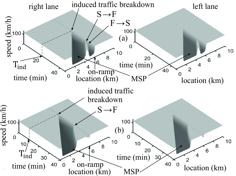
Figure 27: Cooperation of overacceleration in road lane and due to lane-changing leading to S$\rightarrow$F instability on two-lane road with on-ramp bottleneck at $x_{\rm on}=$ 6 km. Simulations with model (1)–(14) at $\tau_{\rm G}=$ 1.4 s made on two-lane road at $q_{\rm in}=$ 2400 (vehicles/h)/lane, $q_{\rm on}=$ 495 vehicles/h (a), and $q_{\rm on}=$ 500 vehicles/h (b). Vehicle speed is space and time in the right lane (left subplots) and in the left lane (right subplots). Traffic breakdown has been induced in free flow at $T_{\rm ind}=$ 20 min (a) and $T_{\rm ind}=$ 10 min (b) through application of addition on-ramp inflow impulse $\Delta q_{\rm on}=$ 1000 vehicles/h of duration $\Delta t=$ 1 min. Spontaneous S$\rightarrow$F and F$\rightarrow$S transitions at the bottleneck are labeled by arrows S$\rightarrow$F and F$\rightarrow$S, respectively. MSP emerges at the bottleneck due to the development of the S$\rightarrow$F instability. Other model parameters are the same as those in Figs. 10(c)–10(e).

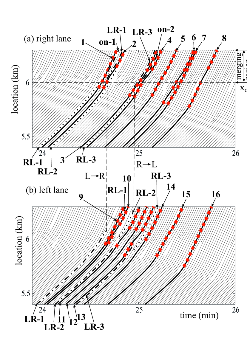
Figure 28: Continuation of Fig. 27(b). (a), (b) Simulated vehicle trajectories in synchronized flow in the right lane (a) and left lane (b). One of the L$\rightarrow$R lane-changing effects (for vehicle LR-1) is marked by dashed vertical line L$\rightarrow$R. One of the R$\rightarrow$L lane-changing effects (for vehicle RL-3) is marked by dashed vertical line R$\rightarrow$L. Part of trajectories within which condition $a_{\rm OA}>0$ is satisfied are marked through colored red squares. Some of the vehicle trajectories used for explanations in text have been highlighted by bold as follows: solid trajectories – vehicles that do not change lane, dotted trajectories – R$\rightarrow$L lane-changing, dashed-dotted trajectories – L$\rightarrow$R lane-changing, dashed trajectories – on-ramp vehicles.

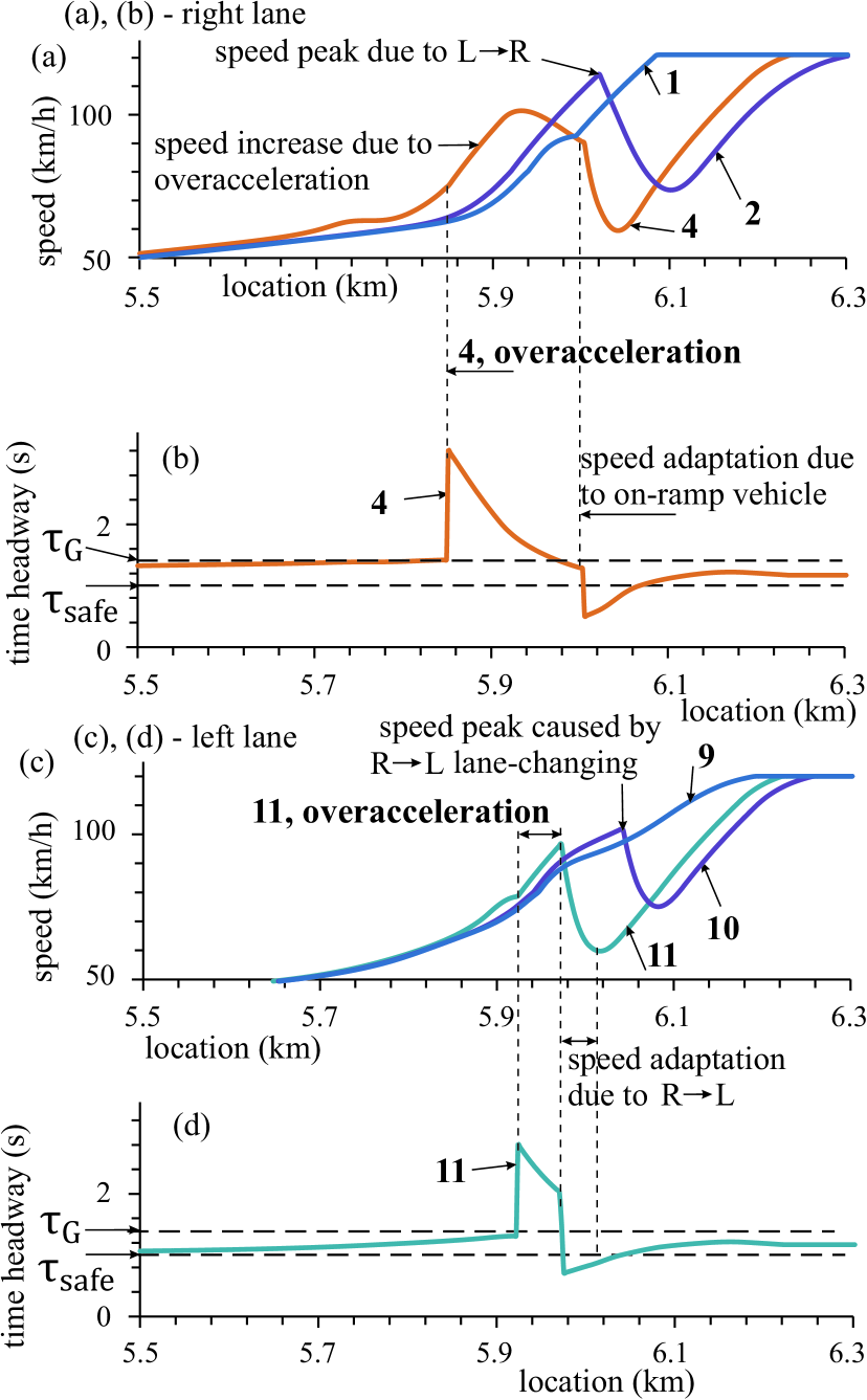
Figure 29: Continuation of Fig. 28. Speed peak in the right lane initiating S$\rightarrow$F instability in the right lane and the beginning of S$\rightarrow$F instability in the left lane through overacceleration caused by L$\rightarrow$R lane-changing. Microscopic vehicle speeds (a), (c) and time headway (b), (d) for right lane (a), (b) and left lane (c), (d) for some of the vehicles whose trajectories are labeled by the same numbers as those in Fig. 28, respectively.

As in stochastic models Kerner2015_SF , the S$\rightarrow$F instability at the bottleneck is initiated spontaneously by a $``$speed peak” (Fig. 29(a)). Vehicle 1 is moving in the right lane and has reached the downstream boundary of synchronized flow. Therefore, vehicle 1 accelerates from the speed inside synchronized flow to free flow. Vehicle 2, following vehicle 1, also starts to accelerate. However, vehicle LR-1 that has changed from the left lane (Fig. 28(a)) forces vehicle 2 to decelerate, creating the speed peak (labeled in Fig. 29(a) by $``$speed peak due to L$\rightarrow$R”).

In this paper, we have revealed that overacceleration cooperation (Secs. IV and V.2) effects crucially on microscopic traffic dynamics of the S$\rightarrow$F instability. We limit a further consideration of the case shown in Fig. 27(b).

VIII.2.1 Effect of lane-changing and merging of on-ramp vehicles in right lane

In the right lane, the S$\rightarrow$F instability is caused by overacceleration cooperation through R$\rightarrow$L lane-changing and overacceleration $a_{\rm OA}$ in road lane. Contrarily, speed adaptation that occurs through the merging of on-ramp vehicles together with L$\rightarrow$R lane-changing tries to prevent the S$\rightarrow$F instability development [Figs. 28–30].

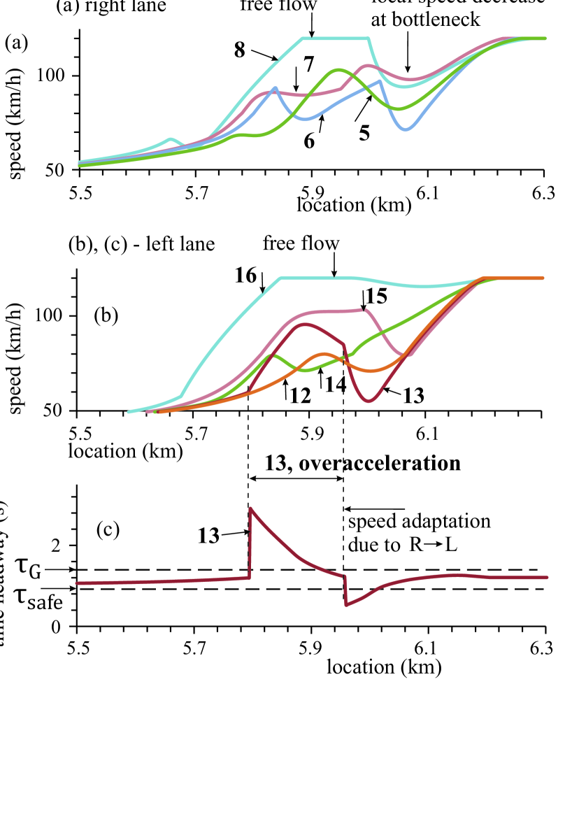
Figure 30: Continuation of Fig. 28. Development of S$\rightarrow$F instability in right lane (a) and left lane (b), (c): Microscopic vehicle speeds (a), (b) and time headway (c) for some of the vehicles whose trajectories are labeled by the same numbers as those in Fig. 28, respectively.

Indeed, after L$\rightarrow$R lane-changing [vehicle LR-3 in Fig. 28(a)] vehicles 3 and RL-3 following vehicle LR-3 in the right lane should decelerate adapting their speeds to the speed of vehicle LR-3. This causes R$\rightarrow$L lane-changing of vehicle RL-3 [Fig. 28(a)]. In its turn, this R$\rightarrow$L lane-changing results in time headway increase for vehicle 4 in the right lane [Fig. 29(b)] and, therefore, in overacceleration of vehicle 4 [$``$4, overacceleration” in Figs. 29(a) and 29(b)]. Overacceleration of vehicle 4 as well as the subsequent acceleration of some following vehicles causes a local speed increase upstream of the on-ramp merging region [$``$speed increase due to overacceleration” in Fig. 29(a)]. However, later due to on-ramp vehicle merging [vehicle on-2 in Fig. 28(a)], vehicle 4 must decelerate, i.e., speed adaptation effect is realized [$``$speed adaptation due to on-ramp vehicle” in Figs. 29(a) and 29(b)]. For this reason, the local speed increase upstream of the on-ramp merging region changes to a local speed decrease within the on-ramp merging region. Rather than the interruption of the S$\rightarrow$F instability, this competition of overacceleration and speed adaptation leads only to a decrease in the growth of the S$\rightarrow$F instability .

The decrease in the growth of a sequence of the local speed increase and decrease explained for vehicle 4 occurs several times upstream of the bottleneck [vehicles 5–7 in Fig. 30(a)]. Finally, the S$\rightarrow$F instability is finished by the S$\rightarrow$F transition at the bottleneck [vehicle 8 in Fig. 30(a)] and the formation of a local speed decrease in free flow upstream of the bottleneck caused mostly by on-ramp vehicles [$``$local speed decrease at bottleneck” in Fig. 30(a)].

VIII.2.2 Emergence of speed peak in left lane

Vehicle 9 accelerates within the downstream boundary of the synchronized flow to free flow downstream [Fig. 29(c)]. Vehicle 10 that follows vehicle 9 also starts to accelerate within the downstream boundary of the synchronized flow. However, a slower moving vehicle RL-1 that has changed from the right lane [vehicle RL-1 in Fig. 28(b)] forces vehicle 10 to decelerate, creating the speed peak on vehicle trajectory 10 [$``$speed peak caused by R$\rightarrow$L lane-changing” in Fig. 29(c)].

VIII.2.3 Effect of lane-changing on S$\rightarrow$F instability in left lane

In the left lane, the S$\rightarrow$F instability is caused by overacceleration cooperation through L$\rightarrow$R lane-changing and overacceleration $a_{\rm OA}$ in road lane. Contrarily, speed adaptation through R$\rightarrow$L lane-changing tries to interrupt the S$\rightarrow$F instability development.

Indeed, because upstream of the speed peak in the left lane the speed decreases, L$\rightarrow$R lane-changing is realized [vehicle LR-2 in Fig. 28(b)]. This results in a time-headway increase for vehicle 11 [Fig. 29(d)] and, therefore, in overacceleration of vehicle 11 [$``$11, overacceleration” in Fig. 29(c)]. Shortly afterward, however, vehicle RL-2 changes from the right lane to the left lane in front of vehicle 11 (Fig. 28). This R$\rightarrow$L lane-changing causes speed adaptation of vehicle 11 [$``$speed adaptation due to R$\rightarrow$L” in Figs. 29(c) and 29(d)].

Thus, there is a sequence of the local speed increase with the following speed decrease caused by speed adaptation. As in the right lane (Sec. VIII.2.1), the local speed increase caused by overacceleration propagates upstream and it can become lower for some of the following vehicles moving upstream of vehicle 11 [e.g., vehicles 12 and 14 in Fig. 30(b)]. Nevertheless, for other vehicles overacceleration leads to the growth of the local speed increase [vehicle 13 in Fig. 30(b)]. This occurs when due to L$\rightarrow$R lane-changing [vehicle LR-3 in Fig. 28(b)] time-headway increases considerably [vehicle 13 in Fig. 30(c)] leading to a greater overacceleration [$``$13, overacceleration” in Figs. 30(b) and 30(c)]. On average due to overacceleration the local speed increase grows upstream [vehicles 13 and 15 in Fig. 30(b)]. Finally, the S$\rightarrow$F instability is finished by the S$\rightarrow$F transition in the left lane [vehicle 16 in Fig. 30(b)].

IX Discussion

IX.1 Microscopic behaviors of vehicle motion as the cause of overacceleration

The behavioral origin of the discontinuous character of overacceleration applied in Eq. (4) has already been explained in Kerner2023B . As we explain here, all other overacceleration mechanisms as well as overacceleration cooperation found above are caused by microscopic behaviors of vehicle motion used in model (1)–(13).

IX.1.1 Competition of speed adaptation with safety acceleration

In Figs. 3, 5, and 7 we have shown that vehicle 1, which must break while approaching slower on-ramp vehicle on-1, accelerates later through safety acceleration. This reflects the vehicle’s desire to move in free flow. However, the breaking of vehicle 1 forces vehicles following vehicle 1 to decelerate; this speed adaptation is the opposite effect to safety acceleration.

When for any vehicle speed within the local speed decrease at the bottleneck speed adaptation is on average stronger than safety acceleration, then safety acceleration cannot prevent congested traffic at the bottleneck. This is independent of the speed within the local speed decrease at the bottleneck (Fig. 2). In this case, safety acceleration does not lead to a nucleation character of traffic breakdown at the bottleneck and, therefore, safety acceleration cannot be considered overacceleration (Sec. III.1).

At other traffic parameters (Secs. III.2 and III.3) speed adaptation is on average weaker than safety acceleration at high enough speeds only, whereas at a low enough speed speed adaptation becomes stronger than safety acceleration. Then safety acceleration does prevent congested traffic at the bottleneck at high enough speeds within local speed decrease at the bottleneck: Safety acceleration does lead to the nucleation character of traffic breakdown at the bottleneck (Figs. 4 and 6). In these cases, in accordance with overacceleration definition, safety acceleration is overacceleration.

IX.1.2 Suppression of speed adaptation within indifferent zone through overacceleration

We consider a vehicle that approaches the local speed decrease at the bottleneck while moving still upstream of the bottleneck within the indifferent zone $g_{\rm safe}\leq g\leq G$. When condition $\alpha=0$ (15) has been assumed (Sec. IX.1.1), then the speed adaptation effect (16) can be stronger than safety acceleration at any speed leading to the absence of overacceleration (Sec. III.1).

Contrarily, under opposite condition $\alpha\neq 0$ due to overacceleration $a_{\rm OA}$ (4) vehicle tries to escape from the local speed decrease at the bottleneck. This overacceleration can suppress speed adaptation within the indifferent zone $g_{\rm safe}\leq g\leq G$ as long as in (4) speed $v\geq v_{\rm syn}$. The suppression of speed adaptation through overacceleration $a_{\rm OA}$ (4), (6) causes the maintaining of free flow at the bottleneck within a considerable larger flow-rate range [Figs. 21(c) and 21(d)] in comparison with the hypothetical case $\alpha=0$ (15) [Fig. 21(b)].

IX.1.3 Overacceleration cooperation in road lane

Microscopic vehicle behaviors leading to overacceleration cooperation in road lane (Sec. IV) are as follows: (i) Overacceleration $a_{\rm OA}$ (4), (6) suppresses speed adaptation as explained in Sec. IX.1.2. (ii) Independent of the effect of the suppression of speed adaptation, there is mechanism of overacceleration caused by safety acceleration [$``$1, overacceleration” in Fig. 9]. (iii) Overacceleration caused by safety acceleration is changed to overacceleration $a_{\rm OA}$ just after time headway becomes longer than safe time-headway [$``$1, change of overacceleration” in Fig. 9]. Due to this overacceleration cooperation the maintaining of free flow at the bottleneck is realized within a larger flow-rate range [Fig. 21(d)] in comparison with the case of single overacceleration mechanism $a_{\rm OA}$ [Fig. 21(c)].

IX.1.4 Vehicle breaking capability as reason for critical speed

The suppression of speed adaptation through overacceleration $a_{\rm OA}$ can be realized only when in (4) condition $v\geq v_{\rm syn}$ is satisfied. This can explain the existence of a critical speed for traffic breakdown (Sec. VI.1) as follows. There is a finite breaking capability of a vehicle: The lower the minimum speed $v_{\rm min}$ within the local speed decrease at the bottleneck, the longer the vehicle breaking distance, therefore, the longer the width of the upstream front of the local speed decrease within which the vehicle decelerates. For this reason, the road location, at which condition $v<v_{\rm syn}$ has been just satisfied and, therefore, overacceleration $a_{\rm OA}=$ 0, moves upstream, when $v_{\rm min}$ decreases.

This effect is realized both on single-lane road [Figs. 17(b) and 18(a)] and two-lane road [Figs. 19(a), 19(b), 20(a), and 20(b)]. Thus, the suppression effect of speed adaptation through overacceleration becomes the weaker, the lower the minimum speed $v_{\rm min}$ within the local speed decrease at the bottleneck. For this reason, there should be a critical minimum speed within the local speed decrease at which speed adaptation becomes on average stronger than overacceleration. This leads to traffic breakdown (F$\rightarrow$S transition).

IX.2 Generalization of deterministic model for moving jam simulations

In the deterministic three-phase traffic flow model used for all simulations presented above [Figs. 2–30] we have used values of model parameters at which there is no vehicle overdeceleration and, therefore, no classical traffic flow instability (and no string instability) exists. For this reason, moving jams occur in none of the simulations even when the synchronized flow speed is very low. However, empirical data have shown that moving jams do emerge in synchronized flow when the synchronized flow speed is low enough KernerBook1 . Therefore, to simulate moving jam emergence in deterministic model (1)–(13), as already made in some stochastic three-phase traffic flow models (e.g., KKl ; OA_Stoch ), we assume that dynamic model parameters (at least some of the model parameters) can change at a synchronized flow speed that is less than some characteristic speed denoted by $v_{\rm pinch}$:

$$\mathcal{P}=\left\{\begin{array}[]{ll}\mathcal{P}\ {\rm at}\ v\geq v_{\rm pinch}\\ \mathcal{P}_{\rm pinch}\ {\rm at}\ v<v_{\rm pinch},\\ \end{array}\right.$$ (20)

where $\mathcal{P}$ denotes one of the model parameters $\tau_{\rm G}$, $\tau_{\rm safe}$, $K_{1}$, $K_{2}$, $K_{3}$, $K^{(1)}_{4}$, $K^{(2)}_{4}$, etc. used in model (1)–(13), whereas the subscript $pinch$ in $\mathcal{P}_{\rm pinch}$ is used to distinguish values of the same model parameters for low speeds $v<v_{\rm pinch}$. We assume also that in Eq. (4) condition

$$v_{\rm pinch}<v_{\rm syn}$$ (21)

is satisfied. In the generalized model, rather than functions (14), we use formulations for the speed-functions $G(v)$ and $g_{\rm safe}(v)$  in which at $v\rightarrow 0$ the space gap tends to some minimum gap $g_{\rm min}$ between vehicles : Respectively, in (1)–(13), rather than $g_{\rm safe}=v\tau_{\rm safe}$ and $G=v\tau_{\rm G}$ (14) [Figs. 2–30], we get:

$$g_{\rm safe}=\left\{\begin{array}[]{ll}v\tau_{\rm safe}\ {\rm at}\ v\geq v_{\rm pinch}\\ g_{\rm min}+v\left(\tau_{\rm safe,pinch}-\tau_{\rm min}\right)\ {\rm at}\ v<v_{\rm pinch},\\ \end{array}\right.$$ (22)

$$G=\left\{\begin{array}[]{ll}v\tau_{\rm G}\ {\rm at}\ v\geq v_{\rm pinch}\\ g_{\rm min}+v\left(\tau_{\rm G,pinch}-\tau_{\rm min}\right)\ {\rm at}\ v<v_{\rm pinch},\\ \end{array}\right.$$ (23)

where $\tau_{\rm min}=g_{\rm min}/v_{\rm pinch}$, $g_{\rm min}$ is a parameter.

IX.3 Empirical traffic breakdown: Vehicle overacceleration versus vehicle overdeceleration

In real empirical traffic data, traffic breakdown at a bottleneck is an F$\rightarrow$S transition that exhibits the empirical nucleation nature KernerBook1 . To study whether vehicle overdeceleration caused by driver overreaction in traffic flow consisting of human-driving vehicles (Sec. I) effects on the F$\rightarrow$S transition, we make the following physical modeling.

IX.3.1 Simulations of spontaneous F$\rightarrow$S transition

In model (1)–(10), (14), in which no vehicle overdeceleration occurs, spontaneous traffic breakdown (F$\rightarrow$S transition) is realized after a time delay $T^{\rm(B)}$ [Fig. 31(a)] (see Sec. VI). When we use generalized model (1)–(10), (22), (23) of Sec. IX.2, in which at speeds $v<v_{\rm pinch}$ vehicle overdeceleration does occur, we find that after traffic breakdown has occurred wide moving jams appear almost immediately [Fig. 31(b)]; in this case, at $t>T^{\rm(B)}$ the spatiotemporal distribution of traffic congestion is qualitatively the same as that well-known from standard traffic flow models (e.g., Bando_2 ; Treiber ; KK1994 ; Krauss ; Treiber-Kesting ; Nagatani_R ), in which traffic breakdown is explained by the classical traffic flow instability resulting from vehicle overdeceleration.

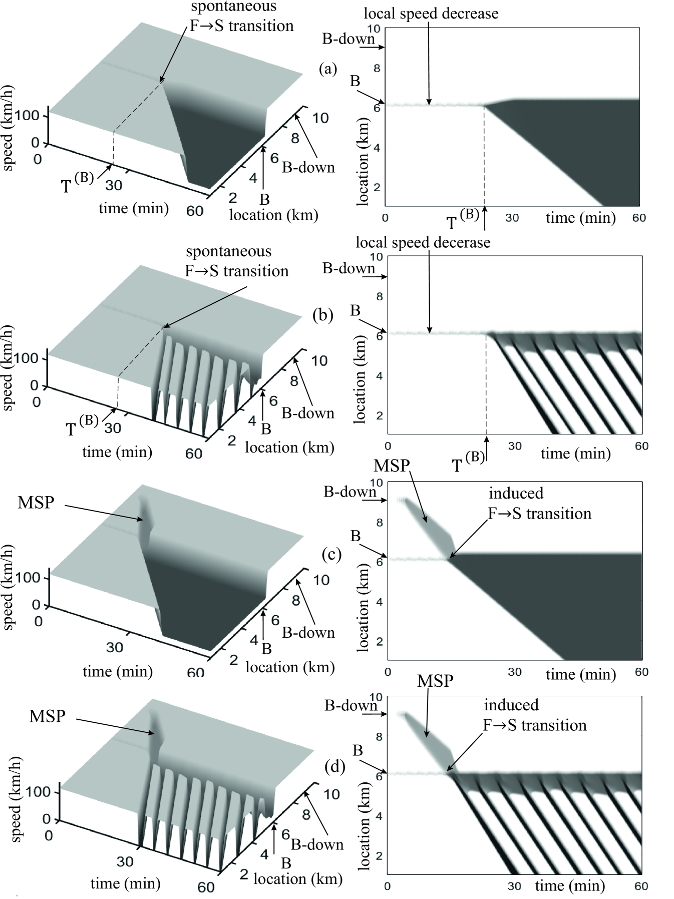
Figure 31: Vehicle overacceleration versus vehicle overdeceleration: What is the cause of real (empirical) traffic breakdown at bottleneck? (a)–(d) Left subplots – simulations of speed in space and time on single-lane road with two on-ramp bottlenecks denoted as $``$B” and $``$B-down” located at $x_{\rm on}=$ 6 km and $x_{\rm on2}=$ 9 km, respectively; right subplots – the same vehicle speed data as those left, respectively, presented by regions with variable shades of gray [shades of gray vary from white to black when the speed decreases from 120 km/h (white) to 0 km/h (black)]; simulations at flow rates: $q_{\rm in}=$ 2250 vehicles/h, on-ramp inflow rates to bottleneck B $q_{\rm on}=$ 568.5 vehicles/h and bottleneck B-down $q_{\rm on2}=$ 0. In (a), (c), simulations of model (1)–(10), (14) with the same model parameters as those in Fig. 8 in which no vehicle overdeceleration is realized. In (b), (d), simulations of model (1)–(10), (22), (23), in which vehicle overdeceleration is realized at $v<v_{\rm pinch}$ with model parameters $g_{\rm min}=$ 5 m, $v_{\rm pinch}=$ 36 km/h, at $v<v_{\rm pinch}$ parameters $K_{3,\rm pinch}=0.1\ s^{-2}$ and $K^{(2)}_{4,\rm pinch}=0.8\ s^{-1}$; other model parameters are the same as those in (a), (c). In (c), (d), MSP (moving synchronized flow pattern) propagating upstream has been induced at downstream bottleneck B-down at $t=$ 2 min through application of on-ramp inflow impulse $\Delta q_{\rm on2}=$ 122 vehicles/h of duration 2 min; while reaching upstream bottleneck B, the MSP induces F$\rightarrow$S transition (traffic breakdown) at upstream bottleneck B.

Therefore, a question can arise: What is a qualitative difference between Fig. 31(b) and related well-known results of the standard traffic flow models? The qualitative difference is that traffic breakdown and its time delay $T^{\rm(B)}$ do not depend whether there is vehicle overdeceleration or not. Indeed, we have found that both the microscopic spatiotemporal development of a local speed decrease in free flow at the bottleneck during time interval $t<T^{\rm(B)}$ and time delay $T^{\rm(B)}$ remain exactly the same in simulations presented in Fig. 31(a) when vehicle overdeceleration does not exist and in Fig. 31(b) when vehicle overdeceleration does exist: Vehicle overdeceleration in generalized model (1)–(10), (22), (23) applied in Fig. 31(b) does not influence on the microscopic features of the development of the F$\rightarrow$S transition (traffic breakdown) at all.

Thus, the microscopic features of traffic breakdown do not depend on whether vehicle overdeceleration is incorporated in the three-phase traffic flow model or not: The physics of the F$\rightarrow$S transition is solely determined by vehicle overacceleration. The F$\rightarrow$S transition leads to the emergence of synchronized flow at the bottleneck. Vehicle overdeceleration occurring in this synchronized flow causes the classical traffic flow instability resulting in the emergence of wide moving jams (called as S$\rightarrow$J transitions): Wide moving jams result from a sequence of F$\rightarrow$S$\rightarrow$J transitions.

IX.3.2 Simulations of empirical induced F$\rightarrow$S transition

For a deeper understanding of the effect of vehicle overdeceleration on real (empirical) vehicular traffic, we simulate empirical induced F$\rightarrow$S transition shown in Fig. 1(a) with either model (1)–(10), (14) [Fig. 31(c)] or with generalized model (1)–(10), (22), (23) [Fig. 31(d)].

For physical modeling of empirical data in Fig. 1(a) we use the fact that there is a long time delay $T^{\rm(B)}\approx$ 24 min of the F$\rightarrow$S transition in both Figs. 31(a) and 31(b). Therefore, free flow at bottleneck B is in metastable state with respect to the F$\rightarrow$S transition at $t<T^{\rm(B)}$. With the use of a short on-ramp inflow impulse applied to downstream on-ramp (B-down) we induce an MSP that reaches upstream bottleneck B at $t<T^{\rm(B)}$. The MSP induces traffic breakdown at bottleneck B [Figs. 31(c) and 31(d)]. Rather than on dynamics of the F$\rightarrow$S transition, vehicle overdeceleration effects only on the congested pattern resulting from the F$\rightarrow$S transition: When model (1)–(10), (14) is used, in which no vehicle overdeceleration is realized, then either spontaneous or induced F$\rightarrow$S transition causes the occurrence of the WSP in which no wide moving jams occur [Figs. 31(a) and 31(c)]; this is independent of how low synchronized flow speed is within the WSP. In contrast, when model (1)–(10), (22), (23) is used, in which vehicle overdeceleration can occur, then wide moving jams spontaneously emerge in low-speed synchronized flow with the speed $v<v_{\rm pinch}$; this slow synchronized flow, in turn, originally resulted from either a spontaneous or induced F$\rightarrow$S transition at bottleneck B [Figs. 31(b) and 31(d)].

We can conclude that the occurrence of the F$\rightarrow$S transition is solely determined by vehicle overacceleration: Independent of whether spontaneous [Figs. 31(a) and 31(b)] or induced F$\rightarrow$S transition [Figs. 31(c) and 31(d)] is realized, vehicle overdeceleration does not effect on features of the F$\rightarrow$S transition at the bottleneck.

IX.4 A possible confusion by simulations of traffic congestion

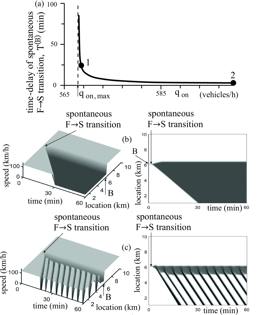
Figure 32: Explanation of a possible confusion by simulations of traffic congestion. Simulations of the same models as those in Figs. 31(a) and 31(b) made on the same single-lane road as well as the same flow rates $q_{\rm in}=$ 2250 vehicles/h and $q_{\rm on2}=$ 0. (a) Time-delay of spontaneous traffic breakdown (F$\rightarrow$S transition) $T^{\rm(B)}$ as function of on-ramp inflow rate $q_{\rm on}$; function $T^{\rm(B)}(q_{\rm on})$ does not depend on whether the model used in Fig. 31(a) or the model used in Fig. 31(b) have been applied; $q_{\rm on,\ max}=$ 568 vehicles/h. (b), (c) Left subplots – simulations of speed in space and time at $q_{\rm on}=$ 600 vehicles/h with the model used in Fig. 31(a) for (b) and with the model used in Fig. 31(b) for (c); right subplots – the same vehicle speed data as those left, respectively, presented by regions with variable shades of gray [shades of gray vary from white to black when the speed decreases from 120 km/h (white) to 0 km/h (black)]. In (a), point 1 is related to $q_{\rm on}=$ 568.5 vehicles/h used in Fig. 31 for which $T^{\rm(B)}\approx$ 24 min, whereas point 2 is related to subplots (b) and (c) for which $T^{\rm(B)}\approx$ 3 min.

To emphasize a possible confusion by simulations of traffic congestion, we consider Fig. 32. The time delay of the spontaneous F$\rightarrow$S-transition $T^{\rm(B)}$ decreases rapidly as the on-ramp inflow rate $q_{\rm on}$, which is larger than $q_{\rm on,\ max}$, continues to increase [Fig. 32(a)]. Therefore, at a large enough flow rate $q_{\rm on}$, time-delay $T^{\rm(B)}$ can be very short. When model (1)–(10), (14) is used, in which there is no vehicle overdeceleration, the result of traffic breakdown simulation [Fig. 32(b)] is qualitatively different from well-known simulation results of the standard traffic flow models in which the classical traffic flow instability in free flow at the bottleneck is the cause of traffic congestion (e.g., Bando_2 ; Treiber ; KK1994 ; Krauss ; Treiber-Kesting ; Nagatani_R ).

Contrarily, when the classical traffic flow instability with wide moving jam emergence (S$\rightarrow$J transitions) is realized in synchronized flow [Fig. 32(c)], then the result of traffic breakdown simulated with generalized model (1)–(10), (22), (23) is qualitatively the same as that simulated with one of the standard traffic flow models. This $``$fraudulent” similarity is because there is almost no time-delay between the F$\rightarrow$S transition and S$\rightarrow$J transition within the sequence of the F$\rightarrow$S$\rightarrow$J transitions: Moving jams occurs already in the emergent synchronized flow. This can lead to a great confusion (and it does very often happen), when a three-phase traffic flow model and a standard traffic flow model are compared.

To solve this confusion, we should understand whether a traffic flow model can simulate the origin of the occurrence of congestion in real (empirical) traffic or not. In other words, the model should be able to simulate the F$\rightarrow$S transition exhibiting the empirical nucleation nature at a bottleneck. This is because this is the basic empirical feature of real traffic breakdown at the bottleneck. As shown in books KernerBook1 ; KernerBook2 ; KernerBook3 ; KernerBook4 , this basic empirical feature of real traffic breakdown (F$\rightarrow$S transition) can be explained by none of the standard traffic flow models of Refs. GM_Com1 ; GM_Com2 ; GM_Com3 ; KS ; KS1 ; KS2 ; KS4 ; Newell1961 ; Newell ; Gipps1981 ; Gipps1986 ; Wiedemann ; Payne_1 ; Payne_2 ; Nagel_S ; Bando_1 ; Bando ; Bando_2 ; Bando_3 ; Nagatani_1 ; Nagatani_2 ; Treiber ; Chen2012A ; Chen2012B ; Chen2014 ; Ashton ; Drew ; Gerlough ; Gazis ; Gartner ; Barcelo ; Elefteriadou ; DaihengNi ; Kessels ; Treiber-Kesting ; Schadschneider ; Chowdhury ; Helbing ; Nagatani_R ; Nagel . This should emphasize why in the three-phase traffic theory the physics of real traffic breakdown is explained through vehicle overacceleration.

Microscopic physics of vehicle overacceleration disclosed in the paper shows that overacceleration is a totally different behavior of microscopic vehicle motion in comparison with overdeceleration caused by driver overreaction in traffic flow of human-driving vehicles. This explains why features of traffic breakdown and highway capacity simulated with three-phase traffic flow models, as shown in the books KernerBook1 ; KernerBook2 ; KernerBook3 ; KernerBook4 , are qualitatively different from features of traffic breakdown and highway capacity simulated with standard traffic flow models (e.g., GM_Com1 ; GM_Com2 ; GM_Com3 ; KS ; KS1 ; KS2 ; KS4 ; Newell1961 ; Newell ; Gipps1981 ; Gipps1986 ; Wiedemann ; Payne_1 ; Payne_2 ; Nagel_S ; Bando_1 ; Bando ; Bando_2 ; Bando_3 ; Nagatani_1 ; Nagatani_2 ; Treiber ; Chen2012A ; Chen2012B ; Chen2014 ; Ashton ; Drew ; Gerlough ; Gazis ; Gartner ; Barcelo ; Elefteriadou ; DaihengNi ; Kessels ; Treiber-Kesting ; Schadschneider ; Chowdhury ; Helbing ; Nagatani_R ; Nagel ).

IX.5 Conclusions

1. For a given flow rate in free flow upstream of an on-ramp bottleneck, the stronger the effect of vehicle overacceleration on traffic flow, the larger the maximum on-ramp flow rate at which free flow can persist at the bottleneck, i.e., the better traffic breakdown can be avoided.

2. In addition to known overacceleration in road lane $a_{\rm OA}$ (4) Kerner2023B , in vehicular traffic there can be at least two mechanisms of vehicle overacceleration in road lane caused by safety acceleration at the bottleneck.

3. Whether an acceleration behavior becomes overacceleration or not depends on traffic characteristics and model parameters. This conclusion is valid for both safety acceleration in road lane and for vehicle acceleration through lane-changing.

4. The microscopic effect of vehicle overacceleration on traffic flow is determined by a spatiotemporal cooperation of different overacceleration mechanisms. The overacceleration cooperation increases the effect of the maintaining of free flow at the bottleneck.

5. Both speed adaptation and overacceleration in road lane can effect qualitatively on overacceleration mechanism caused by lane-changing.

6. The S$\rightarrow$F instability on two-lane road without bottlenecks occurs through cooperation of different overacceleration mechanisms.

7. The S$\rightarrow$F instability on two-lane road with the bottleneck exhibits the following spatiotemporal dynamics.

(i) In the right lane, the S$\rightarrow$F instability is caused by overacceleration cooperation through R$\rightarrow$L lane-changing and overacceleration $a_{\rm OA}$ in road lane. Contrarily, speed adaptation that occurs through merging of on-ramp vehicles together with L$\rightarrow$R lane-changing tries to prevent the S$\rightarrow$F instability development.

(ii) In the left lane, the S$\rightarrow$F instability is caused by overacceleration cooperation through L$\rightarrow$R lane-changing and overacceleration $a_{\rm OA}$ in road lane. Contrarily, speed adaptation through R$\rightarrow$L lane-changing tries to prevent the S$\rightarrow$F instability development.

8. These microscopic features of the effect of vehicle overacceleration on traffic flow (items 1–7 above) are related to traffic flow consisting of human-driving and/or automated-driving vehicles.

References

- (1) R. Herman, E. W. Montroll, R. B. Potts, and R. W. Rothery, Oper. Res. 7, 86 (1959).
- (2) D. C. Gazis, R. Herman, and R. B. Potts, Oper. Res. 7, 499 (1959).
- (3) D. C. Gazis, R. Herman, and R. W. Rothery, Oper. Res. 9, 545 (1961).
- (4) E. Kometani and T. Sasaki, J. Oper. Res. Soc. Jap. 2, 11–26 (1958).
- (5) E. Kometani and T. Sasaki, Oper. Res. 7, 704–720 (1959).
- (6) E. Kometani and T. Sasaki, Oper. Res. Soc. Jap. 3, 176–190 (1961).
- (7) E. Kometani, T. Sasaki, in Theory of Traffic Flow, ed. by R. Herman (Elsevier, Amsterdam, 1961), pp. 105–119.
- (8) G. F. Newell, Oper. Res. 9, 209 (1961).
- (9) G. F. Newell, Transp. Res. B 36, 195 (2002).
- (10) P. G. Gipps, Transp. Res. B 15, 105 (1981).
- (11) P. G. Gipps, Transp. Res. B. 20, 403 (1986).
- (12) R. Wiedemann, Simulation des Verkehrsflusses (University of Karlsruhe, Karlsruhe, 1974).
- (13) H. J. Payne, in Research Directions in Computer Control of Urban Traffic Systems, ed. by W. S. Levine (Am. Soc. of Civil Engineers, New York, 1979), pp. 251–265.
- (14) H. J. Payne, Tran. Res. Rec. 772, 68 (1979).
- (15) K. Nagel and M. Schreckenberg, J. Phys. (France) I 2, 2221 (1992).
- (16) M. Bando, K. Hasebe, A. Nakayama, A. Shibata, Y. Sugiyama, Jpn. J. Appl. Math. 11, 203 (1994).
- (17) M. Bando, K. Hasebe, A. Nakayama, A. Shibata, and Y. Sugiyama, Phys. Rev. E 51, 1035 (1995).
- (18) M. Bando, K. Hasebe, A. Nakayama, A. Shibata, Y. Sugiyama, J. Phys. I France 5, 1389 (1995).
- (19) M. Bando, K. Hasebe, K. Nakanishi, A. Nakayama, Phys. Rev. E 58, 5429 (1998).
- (20) T. Nagatani, Physica A 261, 599 (1998).
- (21) T. Nagatani, Phys. Rev. E 59, 4857 (1999).
- (22) M. Treiber, A. Hennecke, and D. Helbing, Phys. Rev. E 62, 1805 (2000).
- (23) S. Krauß, P. Wagner, and C. Gawron, Phys. Rev. E 55, 5597 (1997).
- (24) R. Jiang, Q. S. Wu, Z. J. Zhu, Phys. Rev. E 64, 017101 (2001).
- (25) R. Barlović, L. Santen, A. Schadschneider, and M. Schreckenberg, Eur. Phys. J. B 5, 793–800 (1998).
- (26) A. Aw and M. Rascle, SIAM J. Appl. Math. 60, 916 (2000).
- (27) D. Chen, J. A. Laval, and S. Ahn, Transp. Res. B 46, 744 (2012).
- (28) D. Chen, J. A. Laval, S. Ahn, and Z. Zheng, Transp. Res. B 46, 1440 (2012).
- (29) D. Chen, S. Ahn, J. Laval, and Z. Zheng, Transp. Res. B 59, 117 (2014).
- (30) W. D. Ashton, The theory of traffic flow (Methuen & Co. London, John Wiley & Sons, New York, 1966).
- (31) D. R. Drew, Traffic Flow Theory and Control (McGraw Hill, New York, 1968).
- (32) D. L. Gerlough, M. J. Huber, Traffic Flow Theory Special Report 165 (Transp. Res. Board, Washington D.C., 1975).
- (33) D. C. Gazis, Traffic Theory (Springer, Berlin, 2002).
- (34) N. H. Gartner, C. J. Messer, A. Rathi (eds.), Traffic Flow Theory (Transportation Research Board, Washington, DC, 2001).
- (35) J. Barceló (ed.), Fundamentals of Traffic Simulation (Springer, Berlin, 2010).
- (36) L. Elefteriadou, An introduction to traffic flow theory, in Springer Optimization and its Applications, Vol. 84 (Springer, Berlin, 2014).
- (37) Daiheng Ni, Traffic Flow Theory: Characteristics, Experimental Methods, and Numerical Techniques (Elsevier, Amsterdam, 2015).
- (38) F. Kessels, Traffic flow modelling (Springer, Berlin, 2019).
- (39) M. Treiber and A. Kesting, Traffic Flow Dynamics (Springer, Berlin, 2013).
- (40) A. Schadschneider, D. Chowdhury, K. Nishinari, Stochastic Transport in Complex Systems (Elsevier Science Inc., New York, 2011).
- (41) D. Chowdhury, L. Santen, and A. Schadschneider, Phys. Rep. 329, 199 (2000).
- (42) D. Helbing, Rev. Mod. Phys. 73, 1067 (2001).
- (43) T. Nagatani, Rep. Prog. Phys. 65, 1331 (2002).
- (44) K. Nagel, P. Wagner, and R. Woesler, Oper. Res. 51, 681 (2003).
- (45) B. S. Kerner and P. Konhäuser, Phys. Rev. E 48, R2335 (1993); 50, 54 (1994); B. S. Kerner, P. Konhäuser, M. Schilke, Phys. Rev. E 51, 6243 (1995).
- (46) P. A. Ioannou and E. B. Kosmatopoulos, Adaptive control, in Wiley Encyclopedia of Electrical and Electronics Engineering, edited by John G. Webster (John Wiley Sons, New York, 2000).
- (47) P. A. Ioannou and C. C. Chien, IEEE Trans. Veh. Technol. 42, 657 (1993).
- (48) W. Levine and M. Athans, IEEE Trans. Automat. Contr. 11, 355 (1966).
- (49) C.-Y. Liang and H. Peng, Veh. Syst. Dyn. 32, 313 (1999).
- (50) C.-Y. Liang and H. Peng, JSME Jnt. J. Ser. C 43, 671 (2000).
- (51) D. Swaroop and J. K. Hedrick, IEEE Trans. Automat. Contr. 41, 349 (1996).
- (52) D. Swaroop, J. K. Hedrick, and S. B. Choi, IEEE Trans. Veh. Technol. 50, 150 (2001).
- (53) S. E. Shladover, Veh. Syst. Dyn. 24, 551 (1995).
- (54) S. E. Shladover, D. Su, and X.-T. Lu, Transp. Res. Rec. 2324, 63 (2012).
- (55) R. Rajamani, Vehicle Dynamics and Control, Mechanical Engineering Series (Springer US, Boston, MA, 2012).
- (56) L. C. Davis, Phys. Rev. E 69, 066110 (2004).
- (57) L. C. Davis, Physica A 405, 128 (2014); 451, 320 (2016); 368, 541 (2006); 361, 606 (2006); 379, 274 (2007); 387, 6395 (2008).
- (58) B. S. Kerner and H. Rehborn, Phys. Rev. Lett. 79, 4030 (1997).
- (59) B. S. Kerner, Phys. Rev. Lett. 81, 3797 (1998).
- (60) B. S. Kerner, Phys. World 12, 25 (1999); Trans. Res. Rec. 1678, 160 (1999); J. Phys. A: Math. Gen. 33, L221 (2000); Phys. Rev. E 65, 046138 (2002); Net. Spat. Econ. 1, 35 (2001); Math. Comput. Model. 35, 481 (2002).
- (61) B. S. Kerner, in Proceedings of the 3rd Symposium on Highway Capacity and Level of Service, edited by R. Rysgaard, Vol 2 (Road Directorate, Ministry of Transport-Denmark, Copenhagen, 1998), pp. 621–642; B. S. Kerner, in Traffic and Granular Flow’97, edited byM. Schreckenberg and D. E.Wolf (Springer, Singapore, 1998), pp. 239–267; B. S. Kerner, in Traffic and Granular Flow’99: Social, Traffic and Granular Dynamics, edited by D. Helbing, H. J. Herrmann, M. Schreckenberg, and D. E. Wolf (Springer, Heidelberg, 2000), pp. 253–284; B. S. Kerner, in Traffic and Transportation Theory in the 21st Century, edited by M. A. P. Taylor (Elsevier, Amsterdam, 2002), pp. 417–439; B. S.Kerner, in Traffic and Granular Flow’01, edited by M. Schreckenberg, Y. Sugiyama, and D. Wolf (Springer, Berlin, 2003), pp. 13–50.
- (62) B. S. Kerner, The Physics of Traffic (Springer, Berlin, New York, 2004).
- (63) B. S. Kerner, Introduction to Modern Traffic Flow Theory and Control (Springer, Berlin, 2009).
- (64) B.S. Kerner, Breakdown in Traffic Networks (Springer, Berlin, New York, 2017).
- (65) B. S. Kerner, Understanding Real Traffic: Paradigm Shift in Transportation Science (Springer, Cham, Switzerland 2021).
- (66) B. S. Kerner, in Complex Dynamics of Traffic Management, edited by B. S. Kerner, Encyclopedia of Complexity and Systems Science Series (Springer, New York, 2019), pp. 195–283 and pp. 387–500.
- (67) B. S. Kerner, H. Rehborn, R.-P. Schäfer, S. L. Klenov, J. Palmer, S. Lorkowski, and N. Witte, Physica A 392, 221 (2013).
- (68) B. S. Kerner, Phys. Rev. E 108, 014302 (2023).
- (69) B. S. Kerner and S. L. Klenov, J. Phys. A: Math. Gen. 35, L31 (2002); Phys. Rev. E 68, 036130 (2003).
- (70) B. S. Kerner and S. L. Klenov, J. Phys. A: Math. Gen. 39, 1775 (2006); Phys. Rev. E 80, 056101 (2009); J. Phys. A: Math. Theor. 43, 425101 (2010); B. S. Kerner, S. L. Klenov, and D. E. Wolf, J. Phys. A: Math. Gen. 35, 9971 (2002); B.S. Kerner, S. L. Klenov, and M. Schreckenberg, Phys. Rev. E 84, 046110 (2011); 89, 052807 (2014); B. S. Kerner, ibid. 85, 036110 (2012); Europhys. Lett. 102, 28010 (2013); Physica A 397, 76 (2014); B. S. Kerner, S. L. Klenov, G. Hermanns, and M. Schreckenberg, ibid. 392, 4083 (2013); B. S. Kerner, Phys. Rev. E 100, 012303 (2019); V. Wiering, S. L. Klenov, B. S. Kerner, and M. Schreckenberg, ibid. 106, 054306 (2022).
- (71) B. S. Kerner, Phys. Rev. E 92, 062827 (2015).
- (72) B. S. Kerner, Phys. Rev. E 97, 042303 (2018); Physica A 562, 125315 (2021).
- (73) Xiaojian Hu, Wei Wang, Haifei Yang, Physica A 391, 5102 (2012).
- (74) Y.-S. Qian, X. Feng, and J.-W. Zeng, Physica A 479, 509 (2017).
- (75) Haifei Yang, Xue Zhai, Changjiang Zheng, Physica A 509, 567 (2018).
- (76) X.-j. Hu, H. Liu, X. Hao, Z. Su, and Z. Yang, Physica A 563, 125495 (2021).
- (77) Zelin Lyu, Xiaojian Hu, Fang Zhang, Tenghui Liu, Zhiwei Cui, Physica A 587, 126471 (2022).
- (78) X.-j. Hu, F. Zhang, J. Lu, M.-y. Liu, Y.-f. Ma, and Q. Wan, Physica A 527, 121176 (2019).
- (79) Jun-Wei Zeng, Yong-Sheng Qian, Sen-Bin Yu, Xu-Ting Wei, Physica A 530, 121567 (2019).
- (80) X.-j. Hu, X.-t. Hao, H. Wang, Z. Su, and F. Zhang, Physica A 545, 123725 (2020).
- (81) Han-Tao Zhao, Lin Lin, Chong-Peng Xu, Zhi-Xiao Li, and Xin Zhao, Physica A 553, 124213 (2020).
- (82) Haifei Yang, Enze Zhao, Yi Zhao, and Yishun Li, Physica A 639, 123725 (2024).
- (83) X.-j. Hu, L.-q. Qiao, X.-t. Hao, C.-x. Lin, and T.-h. Liu, Physica A 605, 127962 (2022).
- (84) Junwei Zeng, Yongsheng Qian, Ziwen Lv, Fan Yin, Leipeng Zhu, Yongzhi Zhang, and Dejie Xu, Physica A 574, 125918 (2021).
- (85) Qiucheng Chen, Shunying Zhu, Jingan Wu, Guojun Chen, and Hong Wang, Physica A 648, 129953 (2024).
- (86) X.-j. Hu and F.-k. Yu, Physica A 659, 127962 (2025).
- (87) B.S. Kerner, Phys. Rev. E 108, 064305 (2023).
- (88) W. Helly, in Proceedings of the Symposium on Theory of Traffic Flow, Research Laboratories, General Motors (Elsevier, Amsterdam, 1959), pp. 207–238.
- (89) H. K. Lee, R. Barlović, M. Schreckenberg, and D. Kim, Phys. Rev. Lett. 92, 238702 (2004).
- (90) B. S. Kerner, German patent publications DE 000010308256A1, 2004; DE 102007008253A1, 2007; DE 102007008257A1, 2007; DE 102007008254A1, 2008; USA patents US 20070150167A1, 2007; US 7451039B2, 2008.
- (91) K. Nagel, D. E. Wolf, P. Wagner, and P. Simon, Phys. Rev. E 58, 1425 (1998).
- (92) M. J. Lighthill and G. B. Whitham, Proc. Roy. Soc. A 229, 317 (1955).
- (93) P. I. Richards, Oper. Res. 4, 42 (1956).
- (94) A. D. May, Traffic Flow Fundamentals (Prentice-Hall, Hoboken, NJ, 1990).
- (95) C. F. Daganzo, Transp. Res. B 28, 269 (1994); 29, 79 (1995).
- (96) Highway Capacity Manual, 6th ed., National Research Council (Transportation Research Board, Washington, DC, 2016).
- (97) M. Takayasu, H. Takayasu, Fractals 1, 860 (1993).