Revisiting CLIP for SF-OSDA: Unleashing Zero-Shot Potential with Adaptive Threshold and Training-Free Feature Filtering
Abstract
Source-Free Unsupervised Open-Set Domain Adaptation (SF-OSDA) methods using CLIP face significant issues: (1) while heavily dependent on domain-specific threshold selection, existing methods employ simple fixed thresholds, underutilizing CLIP’s zero-shot potential in SF-OSDA scenarios; and (2) overlook intrinsic class tendencies while employing complex training to enforce feature separation, incurring deployment costs and feature shifts that compromise CLIP’s generalization ability. To address these issues, we propose CLIPXpert, a novel SF-OSDA approach that integrates two key components: an adaptive thresholding strategy and an unknown class feature filtering module. Specifically, the Box-Cox GMM-Based Adaptive Thresholding (BGAT) module dynamically determines the optimal threshold by estimating sample score distributions, balancing known class recognition and unknown class sample detection. Additionally, the Singular Value Decomposition (SVD)-Based Unknown-Class Feature Filtering (SUFF) module reduces the tendency of unknown class samples towards known classes, improving the separation between known and unknown classes. Experiments show that our source-free and training-free method outperforms state-of-the-art trained approach UOTA by 1.92% on the DomainNet dataset, achieves SOTA-comparable performance on datasets such as Office-Home, and surpasses other SF-OSDA methods. This not only validates the effectiveness of our proposed method but also highlights CLIP’s strong zero-shot potential for SF-OSDA tasks.
1 Introduction
In recent years, the vision-language pre-trained model CLIP [41] has demonstrated exceptional generalization ability across various tasks [49, 5]. Several methods have leveraged CLIP as a backbone for unsupervised domain adaptation [44, 20, 22], aiming to mitigate performance degradation caused by domain shifts between labeled source domain data and unlabeled target domain data. Normally, these approaches assume shared label spaces and require access to the source domain during training. In real-world scenarios, privacy concerns and the complexity of open environments often make the source domain inaccessible. Furthermore, target domains may contain unknown classes that are not present in the source domain. These practical issues have led to increasing interest in the study of source-free unsupervised open-set domain adaptation (SF-OSDA) [30, 48, 25, 39].
Some of these methods replace the source domain with a model trained on the source domain during target domain training [48, 50, 39], while others leverage CLIP’s strong zero-shot capability to perform unsupervised training directly on the target domain [30, 25]. These methods aim to separate the feature distributions of known and unknown class samples during training on the target domain, using thresholding and sample scoring techniques to detect unknown class samples. Despite recent advances achieved by these emerging CLIP-based SF-OSDA methods, they exhibit inherent deficiencies in addressing two pivotal aspects of real-world deployment.
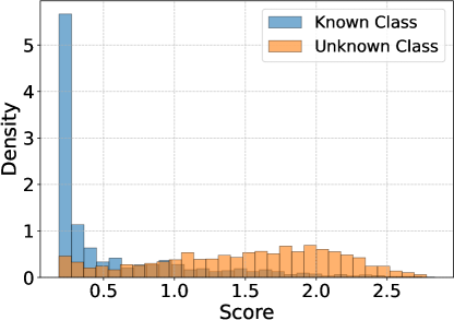
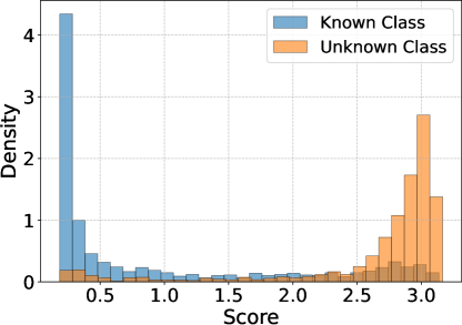
Firstly, CLIP-based SF-OSDA methods achieve promising performance by leveraging zero-shot predictions from known classes to compute sample scores and detect unknown-class samples via a threshold. However, as shown in Figure 1 1(a), their effectiveness heavily relies on threshold selection strategies, with the optimal threshold varying from one domain to another. Existing approaches often adopt simple fixed thresholds [48, 25], failing to fully exploit CLIP’s zero-shot potential in SF-OSDA. For example, in UOTA [30], CLIP’s performance as a baseline is only 66.3%, whereas under the optimal threshold, CLIP achieves 78.7%, which significantly underestimates its capability.
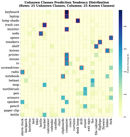
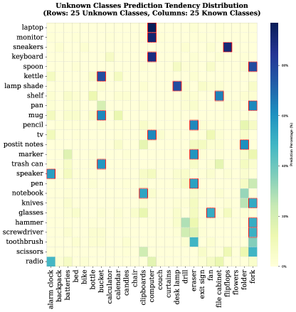
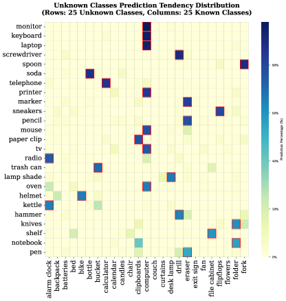
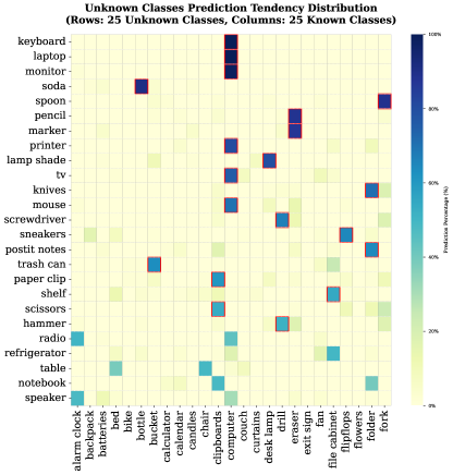
Secondly, in the target dataset, some unknown classes have inherent tendencies towards certain known classes. For example, when the known classes are [“cat”, “airplane”, “train”], an image of a dog, that does not belong to any of these classes, may still be more strongly associated with the “cat” class, leading CLIP to predict it as a cat. As shown in Figure 1 1(b), in the Art domain of the Office-Home dataset, some unknown classes consistently tend to select a specific known class. Such inherent tendencies make it challenging to accurately separate known and unknown class samples based on sample scoring. For example, when using entropy as a sample scoring metric, the dog sample may have a lower entropy due to its stronger association with the cat class. Low-entropy samples are typically considered known classes, leading to classification errors. Previous approaches [48, 25, 30] typically employ complex training strategies to facilitate the separation of features between known and unknown classes. However, this not only requires additional training resources, but it may also alter the original feature distribution of CLIP and reduce the model’s generalization ability.
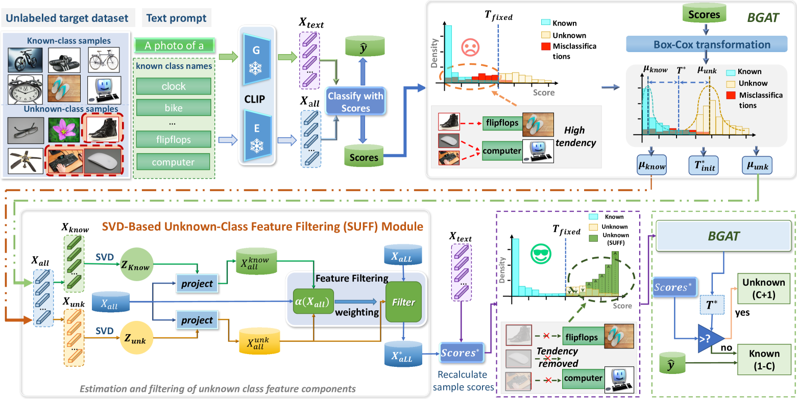
To address these issues, we propose a novel solution, CLIPXpert, which introduces two key components to improve SF-OSDA performance in CLIP zero-shot. Firstly, we present a Box-Cox GMM-Based Adaptive Thresholding (BGAT) module, which refines the thresholding strategy. By applying the Box-Cox transformation to the sample scores and leveraging a Gaussian Mixture Model (GMM) to estimate the distribution of known and unknown classes, BGAT dynamically estimates an optimal threshold. This eliminates the need for manually tuned thresholds and mitigates the performance degradation caused by incorrect threshold choices. Secondly, we introduce a feature filtering module based on Singular Value Decomposition (SVD) [9], named SVD-Based Unknown-Class Feature Filtering (SUFF). This module tackles the class tendency issue in the feature space by reconstructing feature representations and suppressing components that are biased toward the unknown classes. SUFF improves the separability of known and unknown classes, enhancing the model’s open-set detection capabilities without additional training.
Our major contributions are summarized as follows:
-
•
We present CLIPXpert, a source- and training-free open-set domain adaptation framework that achieves competitive performance with state-of-the-art trained methods across multiple benchmarks. To our knowledge, this is the first exploration of an SF-OSDA paradigm requiring neither source data nor training, while fully unleashing CLIP’s zero-shot potential in this scenario.
-
•
We propose a Box-Cox GMM-based Adaptive Thresholding (BGAT) module that not only flexibly models various distributions but also adaptively estimates the optimal threshold under different sample scoring methods. Extensive experiments demonstrate the effectiveness and robustness of the proposed approach.
-
•
We pioneer the exploration of the inherent tendency of unknown classes towards certain known classes, a critical yet underexplored issue that severely impairs detection performance. To address this, we introduce a training-free SVD-based Unknown-Class Feature Filtering (SUFF) module, which effectively mitigates this tendency and enhances detection accuracy.
2 Related Work
Source-Free Unsupervised Open-Set Domain Adaptation. Unsupervised Open Set Domain Adaptation (OSDA) [34, 28, 12] aims to mitigate the decline in model performance caused by distribution discrepancies between the source and target domains, while assuming that the target domain contains unknown categories absent in the source domain. Traditional OSDA methods [26, 4, 39] typically rely on training with both source and target domain data concurrently. However, practical applications may restrict direct access to source domain data during target domain training due to privacy concerns, thereby motivating the development of Source-Free Unsupervised Domain Adaptation (SF-OSDA) [29, 40]. Most existing SF-OSDA [48, 29, 40] approaches substitute source domain samples with models pre-trained on the source domain for target domain training. In recent years, capitalizing on CLIP’s remarkable zero-shot transfer capabilities, some SF-OSDA methods have begun to integrate CLIP with a set of known class names to train directly on unlabeled target domain data [30, 25]. This paper specifically addresses this scenario by proposing a method that requires no training.
Vision-language Models. In recent years, the vision-language pre-trained model CLIP (Contrastive Language-Image Pre-training) [41] has achieved joint embedding in a cross-modal semantic space through contrastive learning on a large-scale dataset of 400 million aligned image-text pairs. Its dual-tower architecture (vision encoder + text encoder) effectively aligns visual and language modalities by maximizing the similarity of positive pairs while minimizing that of negative pairs. The pre-trained CLIP enables zero-shot transfer via cross-modal similarity computation without requiring fine-tuning, demonstrating strong generalization ability to unseen categories in open-world recognition [46, 42, 43]. By designing text prompt templates (e.g., “a photo of a ”) or employing prompt learning techniques [52, 51, 18], CLIP exhibits remarkable robustness and flexibility in downstream tasks, establishing itself as one of the foundational models in computer vision.
3 Methodology
Problem Definition. Given an unlabeled target dataset and a set of known categories , where represents the category name of the -th class, some samples in belong to , while others do not. Our goal is to develop a model that can detect samples in not belonging to the category set and classify them into a new unified class, denoted as class . The remaining samples, which belong to , should be classified into their respective categories. We optimize the model using without updating the model parameters. Finally, we evaluate the performance of the model on .
As shown in Figure 2, the proposed method adaptively estimates the optimal threshold via the Box-Cox GMM-Based Adaptive Thresholding (BGAT) module and filters unknown-class features from using the Training-Free SVD-Based Unknown Feature Filtering (SUFF) module.
3.1 Box-Cox GMM-Based Adaptive Thresholding (BGAT) Module
Traditional open-set domain adaptation methods typically employ fixed thresholds [39, 48] (e.g., Max/2) or global means [4, 26] to distinguish unknown-class samples, which lack theoretical foundation and oversimplify real-world distributions. To investigate a more universal and adaptive threshold calibration strategy, we introduce a statistically grounded approach combining Box-Cox transformation and Gaussian Mixture Models (GMM) [1].
Specifically, as shown in Figure 2, given an unlabeled target dataset and a set of known class names , we perform zero-shot classification on all samples in using CLIP. The classification probabilities for known classes and the detection of unknown samples are computed as follows:
| (1) |
| (2) |
In particular, we define:
| (3) |
where denotes the image encoder, denotes the text encoder, and is the class description sentence with the default prompt “a photo of a”. The threshold is denoted by , and the default sample score is given by:
| (4) |
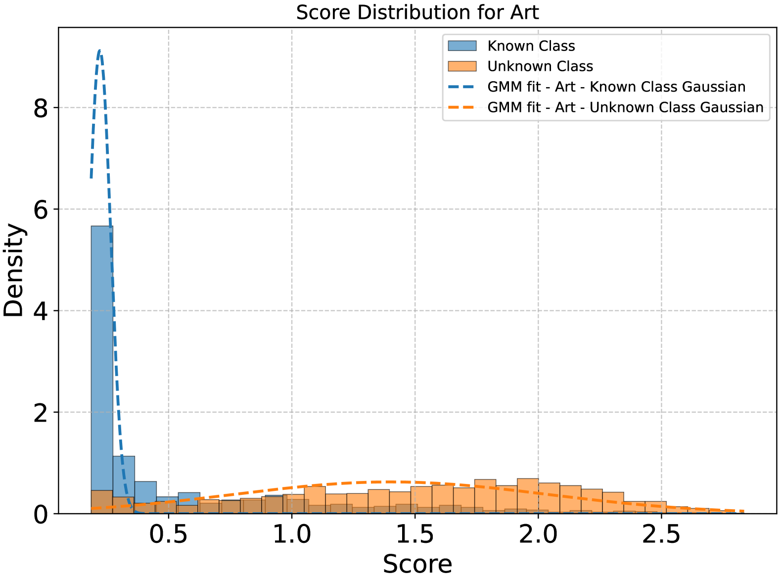
For the scores of the samples, we observe that they typically exhibit a bimodal distribution as shown in Figure 1 1(c). Inspired by prior methods [17, 40], we assume that the score distributions for known-class and unknown-class samples follow Gaussian distributions with different means and variances. Based on this assumption, the optimal threshold can be analytically derived as the intersection of the probability density functions of the two distributions (see Theorem 1 in Appendix A). However, there are two issues in practical datasets that need to be addressed:
Distribution Skewness: Taking the entropy of the samples as an example, as shown in the histogram of Figure 11(c), the entropy of known classes is concentrated near 0 due to the high certainty of most known-class samples. This results in a significant left skew in the distribution, violating the assumption of a Gaussian distribution; Error in GMM Estimation: During the GMM estimation process, errors arise, particularly when the entropy of the samples is highly concentrated. The variance estimation for known classes becomes notably inaccurate, which significantly reduces the accuracy of the intersection points.
Addressing Issue : We apply Box-Cox [3] transformation to mitigate skewness and enforce normality, the transformation of its scores is as follows:
| (5) |
where the optimized parameter is estimated using maximum likelihood [11] as:
| (6) |
Since this data transformation is monotonically increasing, it does not alter the relative ordering of the sample scores. However, it can alleviate the issue of sample scores being too close to known classes, thereby improving the accuracy of mean and variance estimation.
Addressing Issue : After Box-Cox transformation, we fit a two-component GMM to as:
| (7) |
Parameters are estimated via EM [7] and sorted as . However, due to the errors present in the GMM estimation, particularly the tendency for the variance of known classes to be underestimated, and the fact that the intersection point is highly influenced by the variance (which is proven in Theorem 2 of Appendix A), the intersection point may not be the optimal choice in practice.
To address this issue, we adopted a compromise approach by selecting the midpoint of the means, , as the threshold. This choice is motivated by the fact that the mean estimated by GMM is less sensitive to errors than the variance, and using the midpoint enhances the robustness of the threshold. Furthermore, this approach helps improve the robustness of the decision boundary, which is akin to the concept of margin maximization in Support Vector Machines (SVM) [38]. As a result, it can enhance the generalization performance.
Finally, the optimal threshold is derived via inverse Box-Cox transformation as:
| (8) |
In addition, the estimated means of the known and unknown classes also need to be transformed back to the space before the Box-Cox transformation.
3.2 SVD-Based Unknown-Class Feature Filtering (SUFF) Module
Although the BGAT module estimates the optimal threshold , some unknown-class samples may still have low entropy and be misclassified as known-class samples. To resolve this, we propose an SVD-based Unknown Feature Filtering Module (SUFF) that filters out unknown-class features from , improving the separation between known and unknown classes.
Specifically, we first use the known-class mean , the unknown-class mean , and the threshold estimated in Section 3.1 to filter high-confidence known and unknown class sample features. We filter samples with entropy less than or equal to , forming the high-confidence known-class sample feature set ; and we filter samples with entropy greater than, forming the high-confidence unknown-class sample feature set .
Next, we perform SVD on both known-class and unknown-class feature sets to construct their principal component subspaces as:
| (9) |
| (10) |
where and are the singular value matrices. and are the right singular matrices. The smallest dimension is selected such that the cumulative variance contribution satisfies the following:
| (11) |
We retain the top principal components to construct the projection matrices and .
Then, we project all sample features into the constructed known class space and unknown class space as follows:
| (12) |
| (13) |
Next, we analyze the proportion of unknown class features in the samples based on the similarity before and after normalizing the sample feature mapping:
| (14) |
| (15) |
| (16) |
where is temperature coefficient. is set to 1.0 by default and it controls the smoothness of probability distribution.
To remove the unknown-class features from the sample features, we perform a weighted subtraction operation as follows:
| (17) |
Finally, we recompute the sample scores using the filtered features and , and re-estimate the threshold using the BGAT module. The final prediction for each sample is then obtained by combining calculated from the original features and applying Equation 2, which prevents errors in feature filtering from adversely affecting the model’s recognition performance on known classes.
4 Experiments
| Method | E | SF-S | CLIP | TF | Office-Home | VisDA-2017 | ||||||||||||
| C | P | R | A | P | R | A | C | R | A | C | P | AVG | S | |||||
| A | C | P | R | R | ||||||||||||||
| Anna | RN | 64.7 | 66.5 | 71.3 | 69.0 | 63.1 | 65.7 | 73.7 | 68.6 | 76.6 | 76.8 | 73 | 78.7 | 70.64 | - | |||
| USD | 60.1 | 62.6 | 67.8 | 61.1 | 56.3 | 59.1 | 70 | 65.2 | 71.1 | 76.3 | 68.9 | 72.2 | 65.89 | 69.4 | ||||
| LEAD | 61.0 | 65.5 | 64.8 | 60.7 | 59.8 | 57.7 | 70.8 | 68.6 | 75.8 | 76.5 | 70.8 | 74.2 | 67.18 | 74.2 | ||||
| SHOT-O | 56.4 | 60 | 61.8 | 37.7 | 41.5 | 41.4 | 41.8 | 39.8 | 43.6 | 48.4 | 40.9 | 49.7 | 46.92 | 28.1 | ||||
| UMAD + LEAD | 61.3 | 63.3 | 66.7 | 62.6 | 54.6 | 63.5 | 73.6 | 66.2 | 75.6 | 77.3 | 70.7 | 75.1 | 67.54 | 70.2 | ||||
| Co-learn++ | 60.4 | 56.0 | 64.0 | 54.9 | 51 | 58.8 | 77.6 | 72.7 | 83.6 | 78.4 | 75.9 | 77.2 | 67.54 | - | ||||
| CLIPXpert | 72.5 | 61.3 | 80.9 | 81.3 | 74.00 | 85.1 | ||||||||||||
| DIFO-B32 | ViT | 68.2 | 67.2 | 71.9 | 64.5 | 62.1 | 65.3 | 86.2 | 79.3 | 84.4 | 87.9 | 86.1 | 88.3 | 75.95 | - | |||
| ODAwVL(C=15) | 82.3 | 82.2 | 82.1 | 76.5 | 76.5 | 76.8 | 79.3 | 78.6 | 78.9 | 85.5 | 84.8 | 84.6 | 80.67 | 83.8 | ||||
| CLIP + MCM | 74.0 | 68.7 | 77.6 | 77.6 | 74.46 | 80.5 | ||||||||||||
| CLIP + Entropy | 76.4 | 69.6 | 76.1 | 80.1 | 75.52 | 83.1 | ||||||||||||
| CLIP + Energy | 73.3 | 62.8 | 78.5 | 77.1 | 72.90 | 78.9 | ||||||||||||
| CLIPXpert-B32 | 73.2 | 73.5 | 85.6 | 86.3 | 79.66 | 85.89 | ||||||||||||
| COSmo(C=15) | 81.0 | 86.8 | 82.4 | 82.0 | 83.0 | - | ||||||||||||
| UEO | 68.3 | 63.7 | 65.6 | 70.4 | 66.98 | 70.1 | ||||||||||||
| UOTA | 79.1 | 79.1 | 87.0 | 87.4 | 83.15 | 89.7 | ||||||||||||
| CLIPXpert | 78.9 | 74.9 | 85.6 | 85.4 | 81.17 | 87.2 | ||||||||||||
| CLIPXpert (C=15) | 84.8 | 79.4 | 87.0 | 89.9 | 85.27 | N/A | ||||||||||||
| Method | ImageNet | Caltech101 | DTD | EuroSAT | Food101 | Flowres102 | OxfordPets | SUN397 | StandfordCars | UCF101 | AVG |
|---|---|---|---|---|---|---|---|---|---|---|---|
| CLIP + MCM | 61.49 | 81.93 | 59.95 | 51.14 | 74.63 | 67.64 | 65.73 | 65.23 | 51.43 | 68.26 | 64.74 |
| CLIP + Entropy | 61.94 | 84.00 | 60.64 | 51.96 | 76.64 | 68.96 | 69.74 | 65.68 | 53.80 | 71.30 | 66.47 |
| CLIP + Energy | 72.11 | 82.56 | 48.25 | 47.42 | 79.81 | 66.21 | 77.87 | 62.6 | 64.27 | 65.51 | 66.66 |
| UEO | 59.54 | 80.06 | 42.31 | 36.51 | 72.56 | 63.39 | 65.47 | 59.77 | 50.91 | 65.18 | 59.57 |
| CLIPXpert | 71.97 | 89.84 | 62.17 | 51.84 | 86.64 | 68.88 | 77.61 | 70.81 | 55.61 | 76.22 | 71.16 |
4.1 Experimental Settings
Datasets. We evaluate our method on multiple public datasets to assess its effectiveness in open-set domain adaptation (OSDA). For OSDA tasks, we use three benchmark datasets: Office-Home [45] (65 categories, 4 domains), VisDA-2017 [36] (12 categories, synthetic-to-real adaptation), and DomainNet [37] (345 categories, 6 domains). To further test generalization, we select 10 datasets from the Visual Task Adaptation Benchmark (VATB), including ImageNet [8], Caltech101 [10], EuroSAT [15], Food101 [2], Flowers102 [33], OxfordPets [35], SUN397 [47], StandfordCars [19], and DTD [6]. These datasets cover diverse visual tasks with large-scale data and significant domain differences. Known class selection follows the UOTA [30] setting for OSDA datasets, while varying proportions of unknown classes are used for VATB datasets to ensure robustness. More details can be found in Appendix B.1.
Baselines. To the best of our knowledge, the SF-OSDA method, which requires neither source domain data nor training, has not been explored in existing research. Therefore, we select three categories of baseline methods for comparison: CLIP-based zero-shot methods using Maximum Concept Matching (MCM) [31], Entropy [16], and Energy[27] for scoring; Traditional OSDA methods that rely on source domain data or pre-trained models, including ANNA [21], USD [17], LAED [40], SHOT [23], UMAD [24], Co-learn++ [50], DIFO, Cosmo [32], and ODAwVL [48]; Unsupervised target domain methods such as UOTA [30] and UEO [25], which perform training and unknown class detection directly on the target domain. More details can be found in Appendix B.2.
Implementation Details. We use four different backbone networks as image encoders: ResNet-50 [14], ResNet-101 [14], ViT-B/16 [13], and ViT-L/14 [13]. These backbones are selected to ensure consistency with various comparison methods. The specific settings are detailed in the experimental results table. Note that in Table 1, for methods using ResNet, the Office-Home dataset uses ResNet-50, the VisDA-2017 dataset uses ResNet-101, and results without explicit notation in all tables use ViT-B/16. Additionally, our default configuration is = 0.9, a batch size of 32.
4.2 Overall Performance
As shown in Table 1, compared to previous methods using ResNet as the backbone, our approach achieves significant improvements under the same image encoder settings, surpassing LEAD by 6.82% and 10.87% on the OfficeHome and VisDA-2017 datasets, respectively. Furthermore, on the OfficeHome dataset, our performance exceeds that of Co-learn++, which also utilizes the CLIP model, by 6.46%.
Additionally, compared to other CLIP-based methods using ViT as the image encoder, our approach achieves the best performance on the OfficeHome dataset when the number of known classes is 15, outperforming CosMo by 2.23%. When the number of known classes is 25, our method surpasses all approaches except UOTA. However, as shown in Table 3, while our performance is 1.98% and 2.55% lower than UOTA on the OfficeHome and VisDA datasets, we outperform UOTA by 1.92% on the most challenging dataset, DomainNet, and unlike UOTA, our method requires no additional training. Finally, as shown in Table 2, our method outperforms UEO by 11.59% across a more diverse set of 10 VATB datasets and also surpasses other CLIP-based zero-shot OOD methods. Since UEO and the three OOD models lack a threshold computation strategy, we adopt the average value of the target dataset as a unified threshold for detecting unknown-class samples.

| Method | E | DomainNet | ||||||
|---|---|---|---|---|---|---|---|---|
| C | I | P | Q | R | S | AVG | ||
| CLIP + MCM | ViT-L/14 | 75.40 | 66.31 | 73.54 | 38.41 | 79.18 | 74.22 | 67.84 |
| CLIP + Entropy | 74.85 | 65.76 | 73.65 | 38.85 | 78.82 | 73.97 | 67.65 | |
| CLIP + Energy | 69.29 | 59.70 | 67.80 | 34.49 | 75.23 | 67.84 | 62.39 | |
| UEO | 71.23 | 62.78 | 69.12 | 35.83 | 73.4 | 68.62 | 63.50 | |
| UOTA | 82.40 | 68.70 | 77.00 | 35.90 | 85.20 | 77.30 | 71.08 | |
| CLIPXpert | 83.18 | 69.21 | 79.14 | 39.52 | 87.27 | 79.68 | 73.00 | |
4.3 Ablation Study
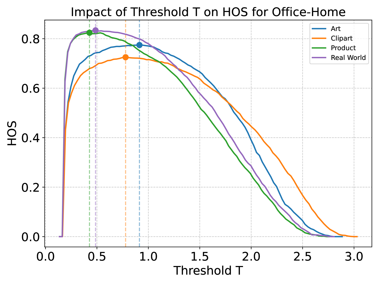
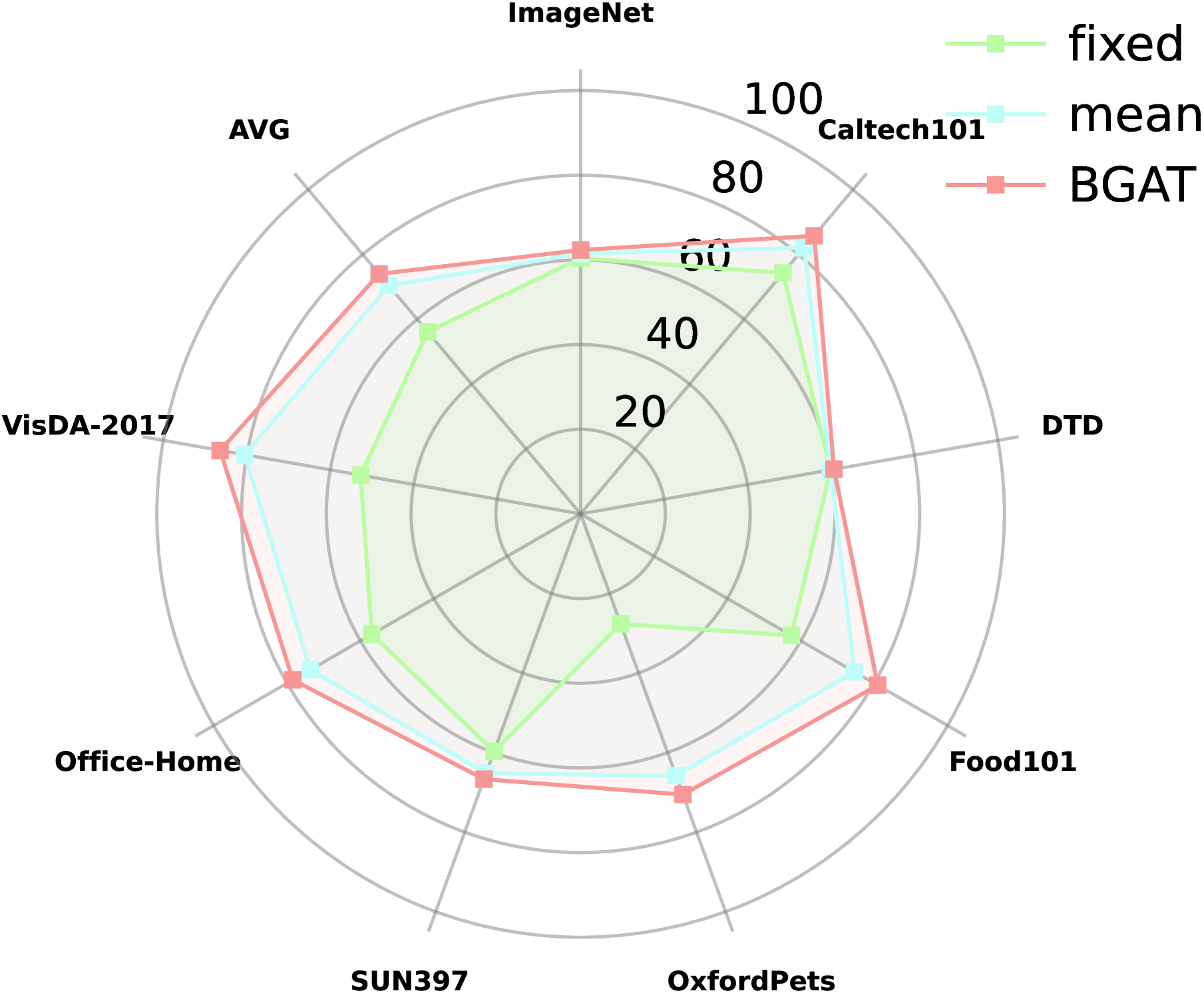
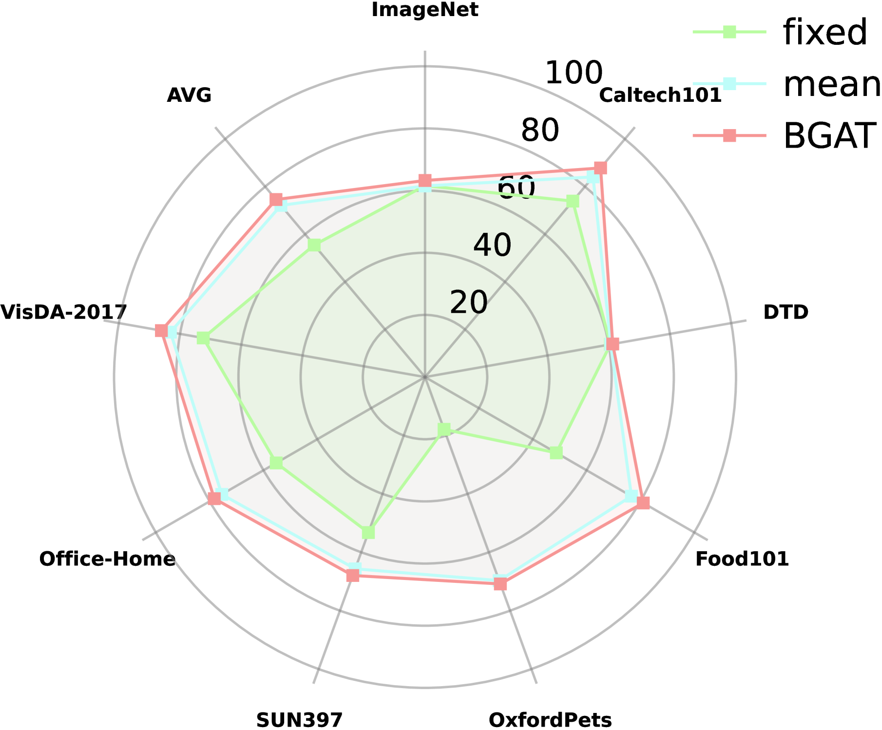
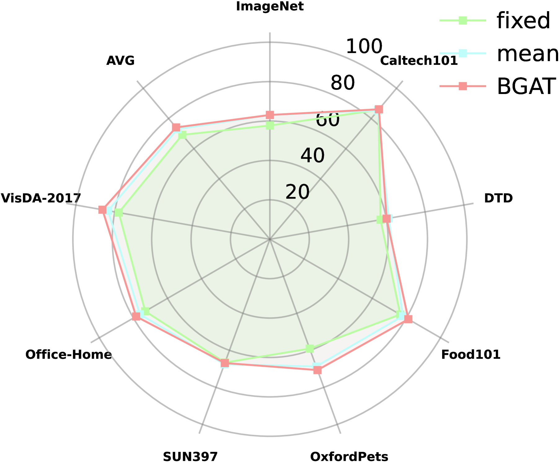
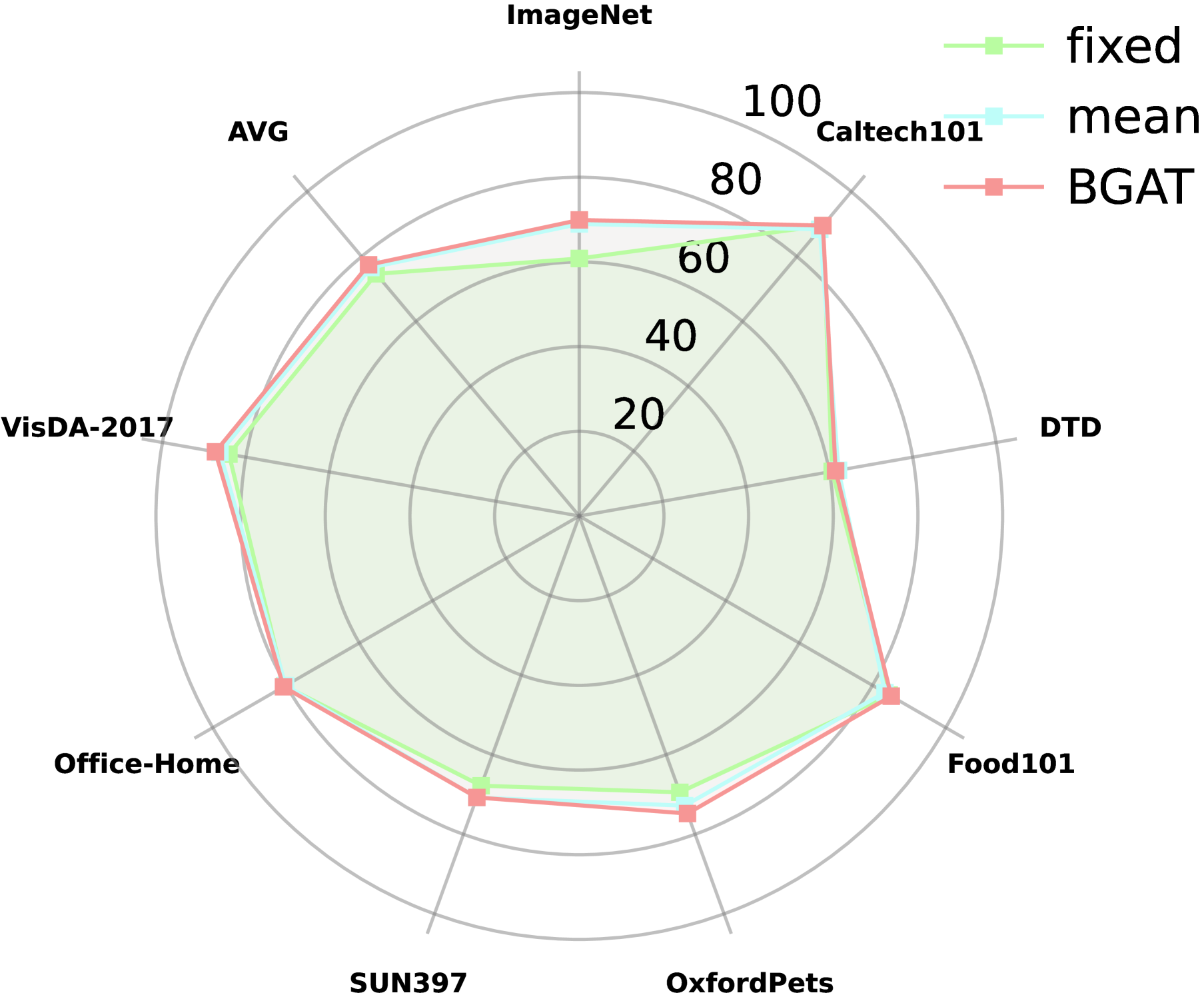
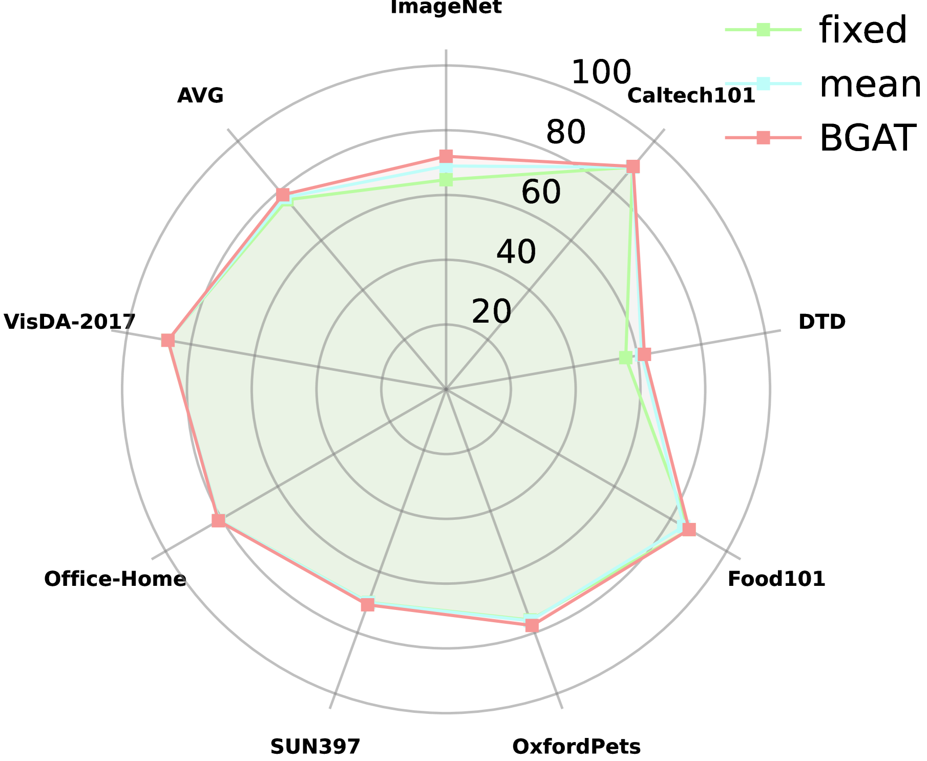
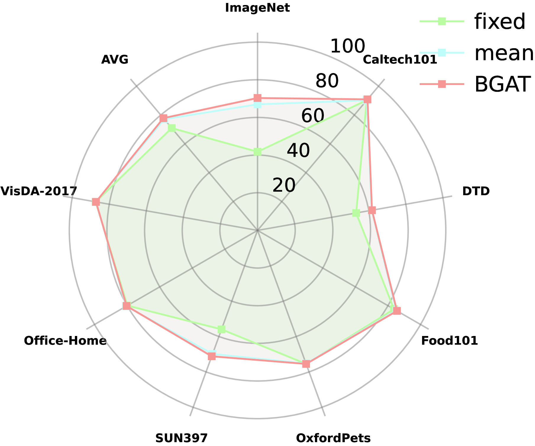
Effectiveness of BGAT. Since CLIP-based unknown class sample detection using scores is sensitive to threshold selection, we compare three different threshold calculation methods across eight datasets: a fixed threshold (max/2), the mean score of the target dataset, and our proposed BGAT. As shown in Figure 3 3, 3 and 3, for the raw CLIP feature-based sample scores, BGAT outperforms the fixed threshold by 17.84%, 19.11%, and 4.90% in terms of MCM, Entropy, and Variance scores(VAR), respectively. It also surpasses the mean threshold by 3.56%, 2.46%, and 1.16%, demonstrating that BGAT significantly improves the performance of CLIP-based sample scoring. Furthermore, as shown in Figure 3 3, 3 and 3, after filtering out unknown class features using the SUFF module, BGAT still surpasses the fixed threshold by 2.80%, 2.01%, and 6.88%, and outperforms the mean threshold by 0.84%, 1.07%, and 0.73%. More details can be found in Appendix B.3.
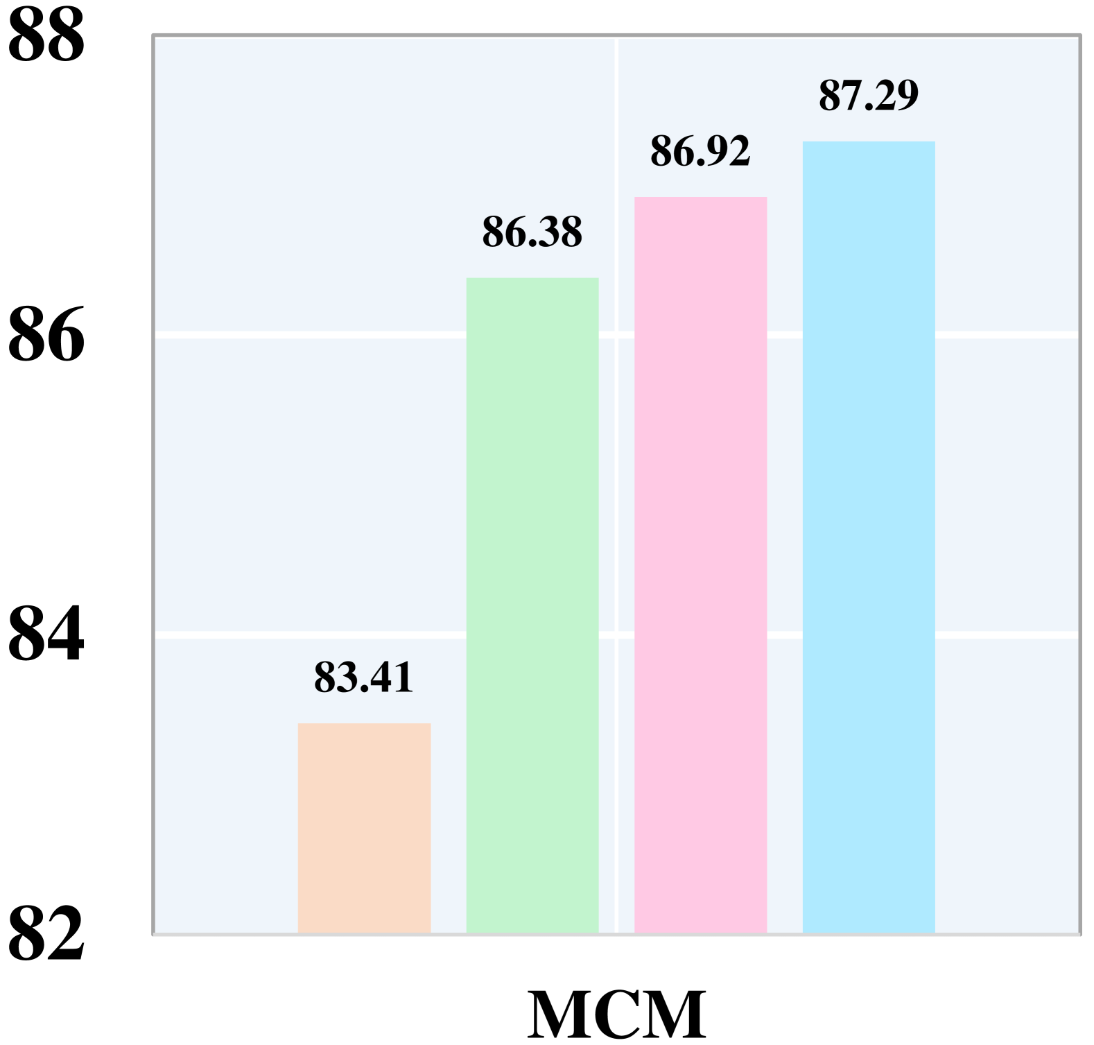
| Score | SUFF | VATB-6 | Office-Home | VisDA-2017 | AVG |
|---|---|---|---|---|---|
| Entropy | 74.24 | 78.26 | 86.09 | 74.57 | |
| 77.59 | 81.16 | 87.17 | 78.42 (+3.85%) | ||
| MCM | 73.95 | 78.41 | 86.38 | 73.97 | |
| 76.68 | 80.68 | 87.29 | 77.44 (+3.47%) | ||
| VAR | 73.92 | 78.39 | 86.30 | 74.09 | |
| 76.89 | 80.30 | 87.15 | 77.82 (+3.72%) |
Effectiveness of SUFF. We conduct experiments on eight datasets to validate the effectiveness of SUFF module by integrating it into CLIP under the BGAT-based thresholding method. As shown in Table 4, compared to raw CLIP without the SUFF module, performance improvements of 3.85%, 3.47%, and 3.72% are achieved under the three scoring methods, respectively. In particular, on ImageNet, the largest data set within VATB, the performance increased by 8.72%, 7.58%, and 7.22% under the three scoring methods (see Table 7 in Appendix B.3 for details).
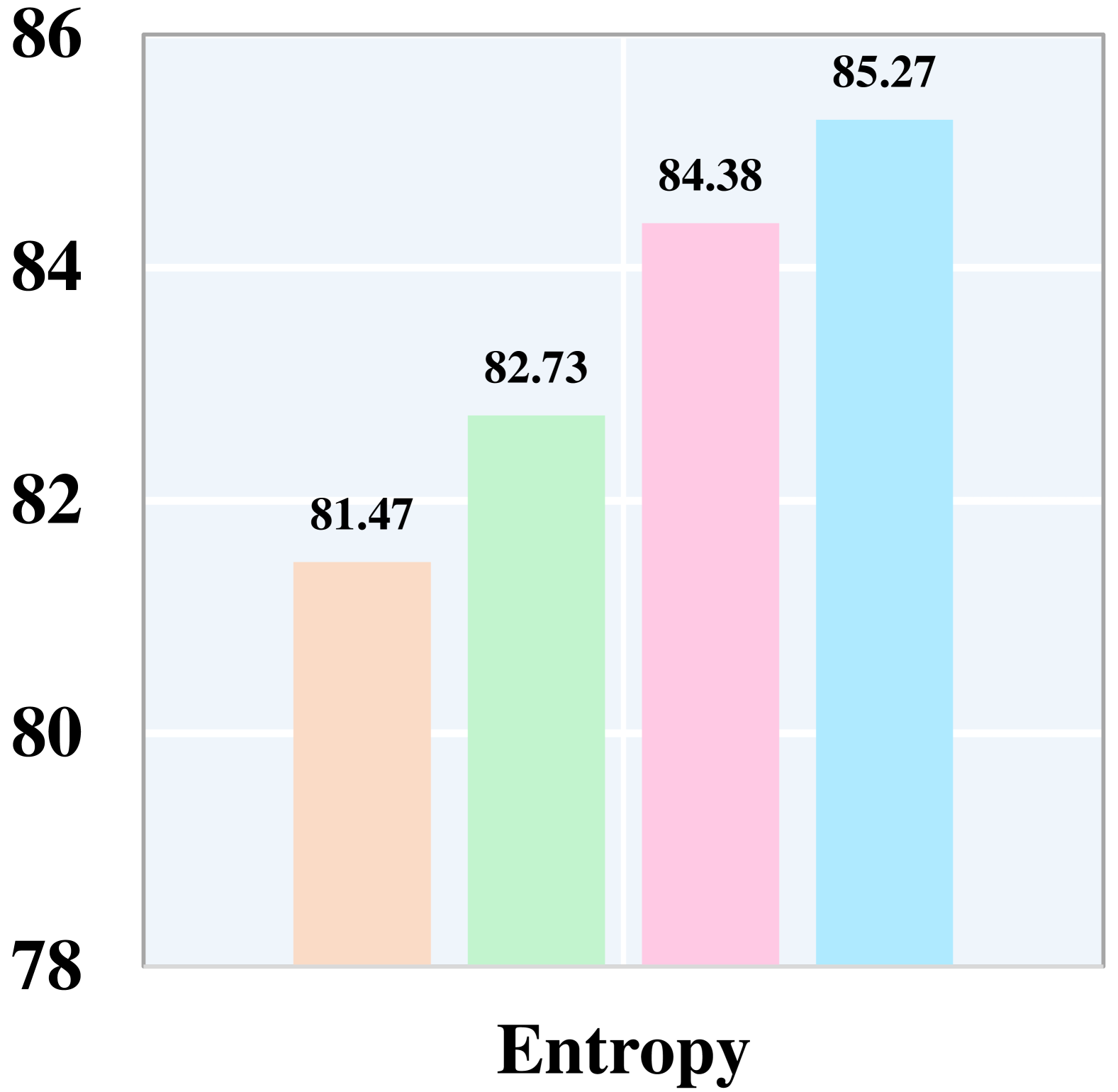
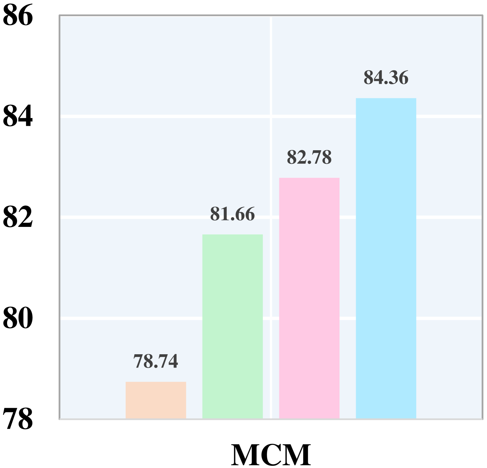
Effectiveness of Box-Cox. We validate the effectiveness of integrating Box-Cox transformation into the BGAT module across four domains of Office-Home dataset and VisDA-2017 dataset. As shown in Figure 4, three sets of sample scores are compared. For the original CLIP model, incorporating the Box-Cox transformation significantly improved performance, yielding average increases of 2.03% on the Office-Home dataset and 1.39% on the VisDA-2017 dataset. Even after applying the SUFF module for feature filtering, the Box-Cox transformation result in additional improvements of 0.95% on Office-Home and 0.13% on VisDA-2017. More details can be found in Appendix B.3.
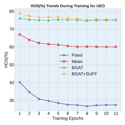
Impact of BGAT and SUFF on UEO. We validate the effectiveness of BGAT and SUFF modules in UEO across four domains of Office-Home dataset. As shown in Figure 6 6(b), considering only the thresholding strategy, BGAT significantly outperforms both fixed and average thresholds, and it demonstrates exceptional robustness during training without the marked performance decline observed with fixed and average thresholds. Moreover, even with early stopping at the first epoch, the performance using BGAT thresholds exceeds that of fixed and average thresholds by 28.96% and 3.58%, respectively. With the incorporation of the SUFF module, performance is further enhanced by 3.59%. More details can be found in Appendix B.3.
4.4 Hyper-parameter Analysis
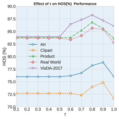
We analyze the impact of the hyperparameter in Equation 11 on model performance across the four domains of the Office-Home and VisDA-2017 datasets. As shown in Figure 6 6(a), when is between 0 and 0.5, few principal components are retained, resulting in limited reconstructed feature information and almost no improvement in model performance. However, when exceeds 0.5, the model performance gradually improves, reaching its optimum at values of 0.8 or 0.9; if is set to 1, too much noise is retained, leading to a decline in performance.
4.5 Case Study
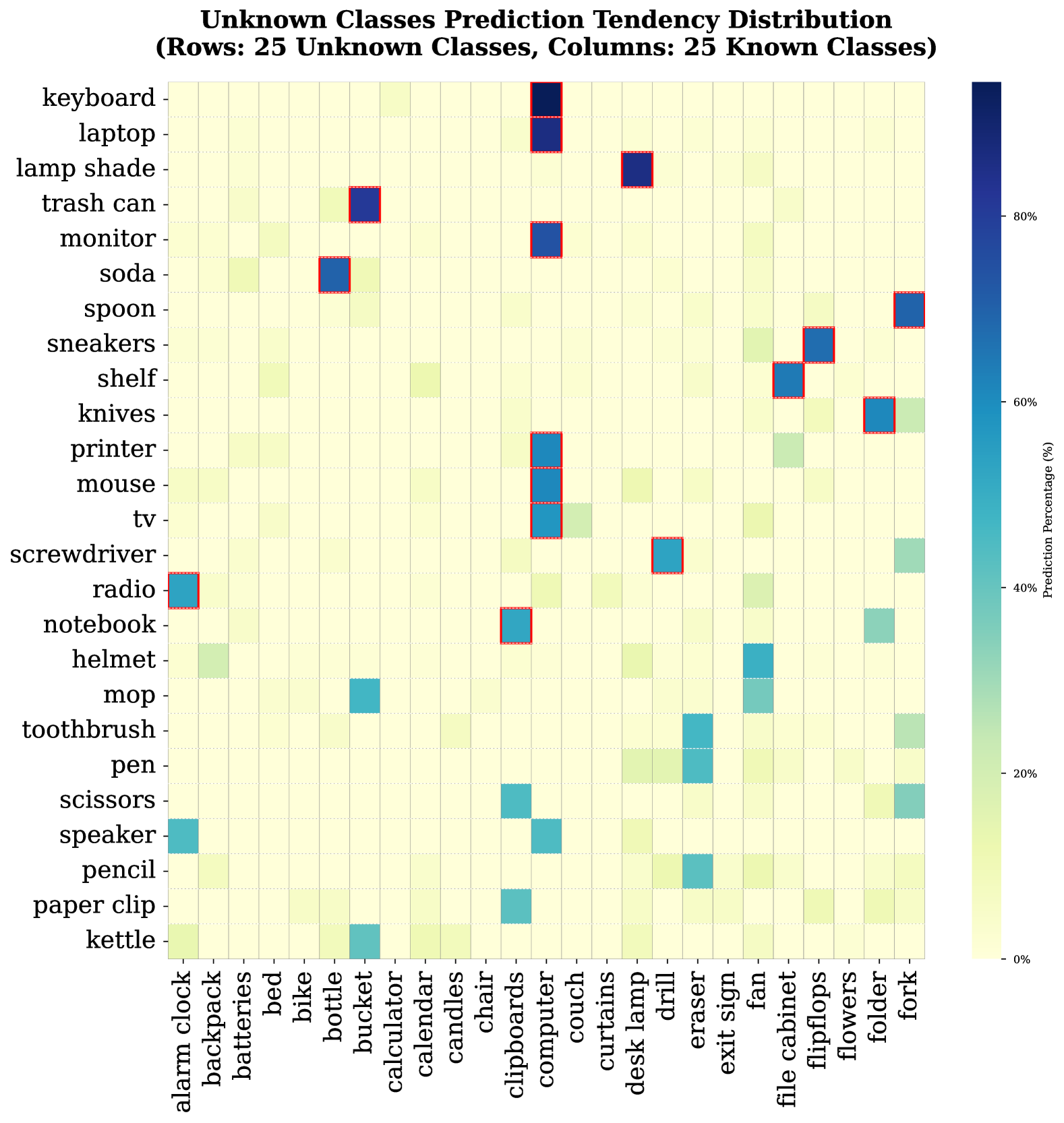
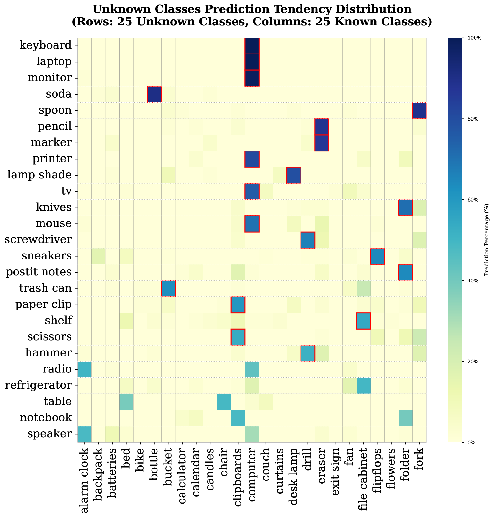
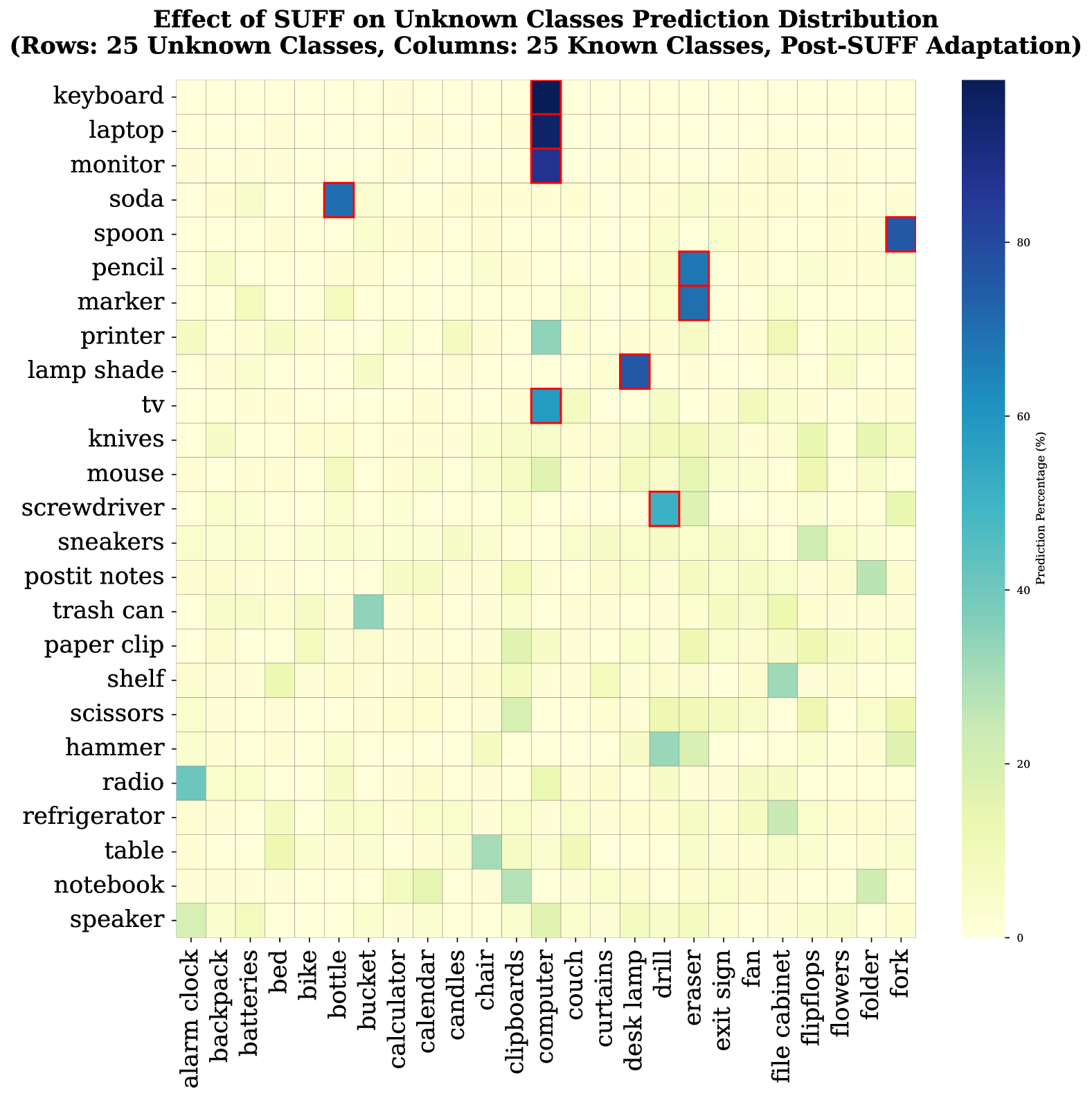
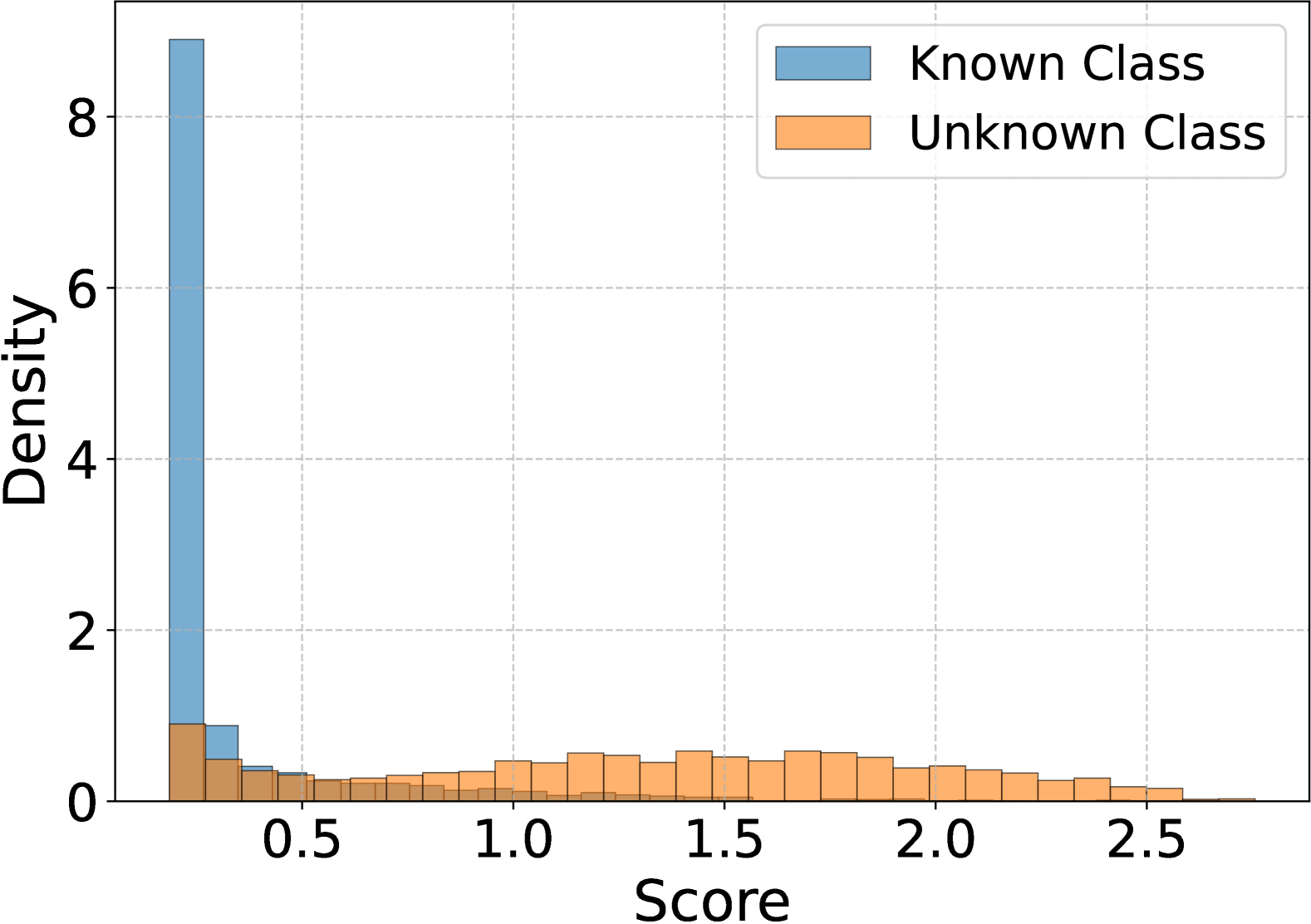
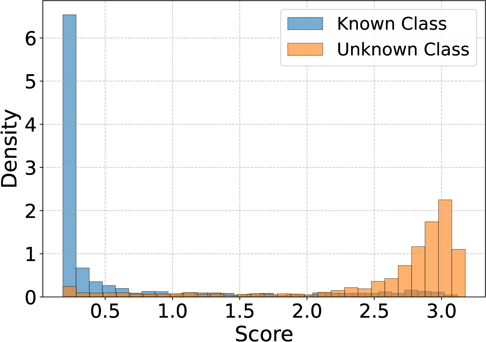
Tendency and Entropy Variation Visualization. We visualize the tendency change of unknown classes towards known classes and the entropy change of samples before and after applying the SUFF module on the Office-Home dataset. As shown in the first row of Figure 7, the SUFF module significantly reduces the number of unknown classes with a tendency towards known classes. Additionally, as shown in the second row of Figure 7, the entropy of the unknown class sample increases after filtering with the SUFF module, leading to a notable improvement in the separability between known and unknown classes.
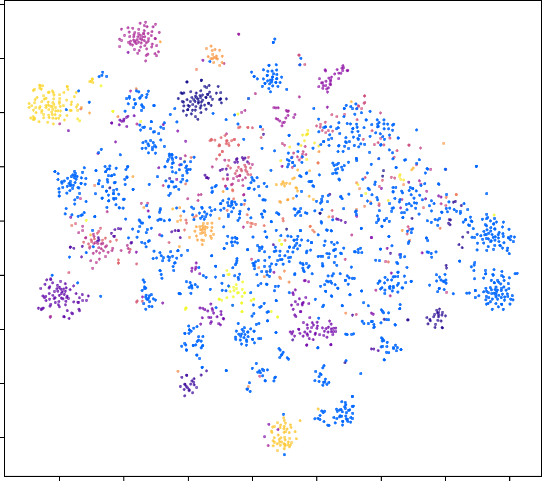
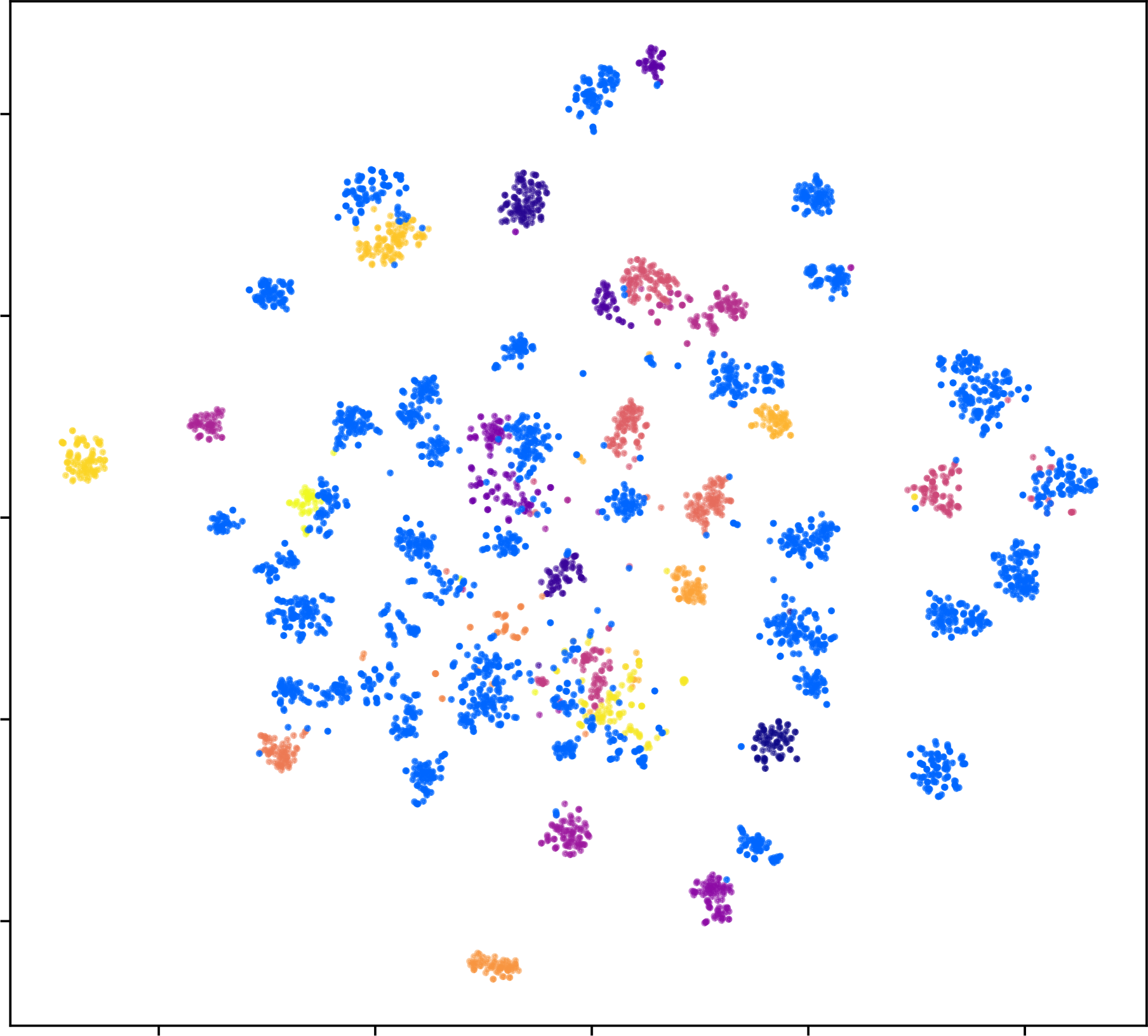
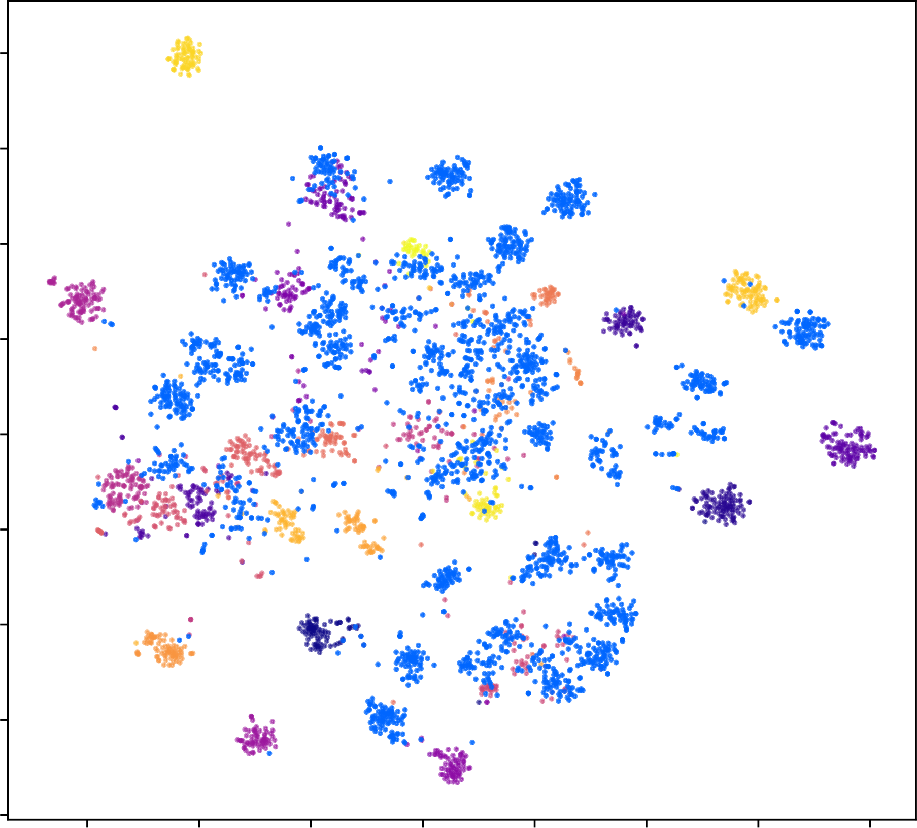
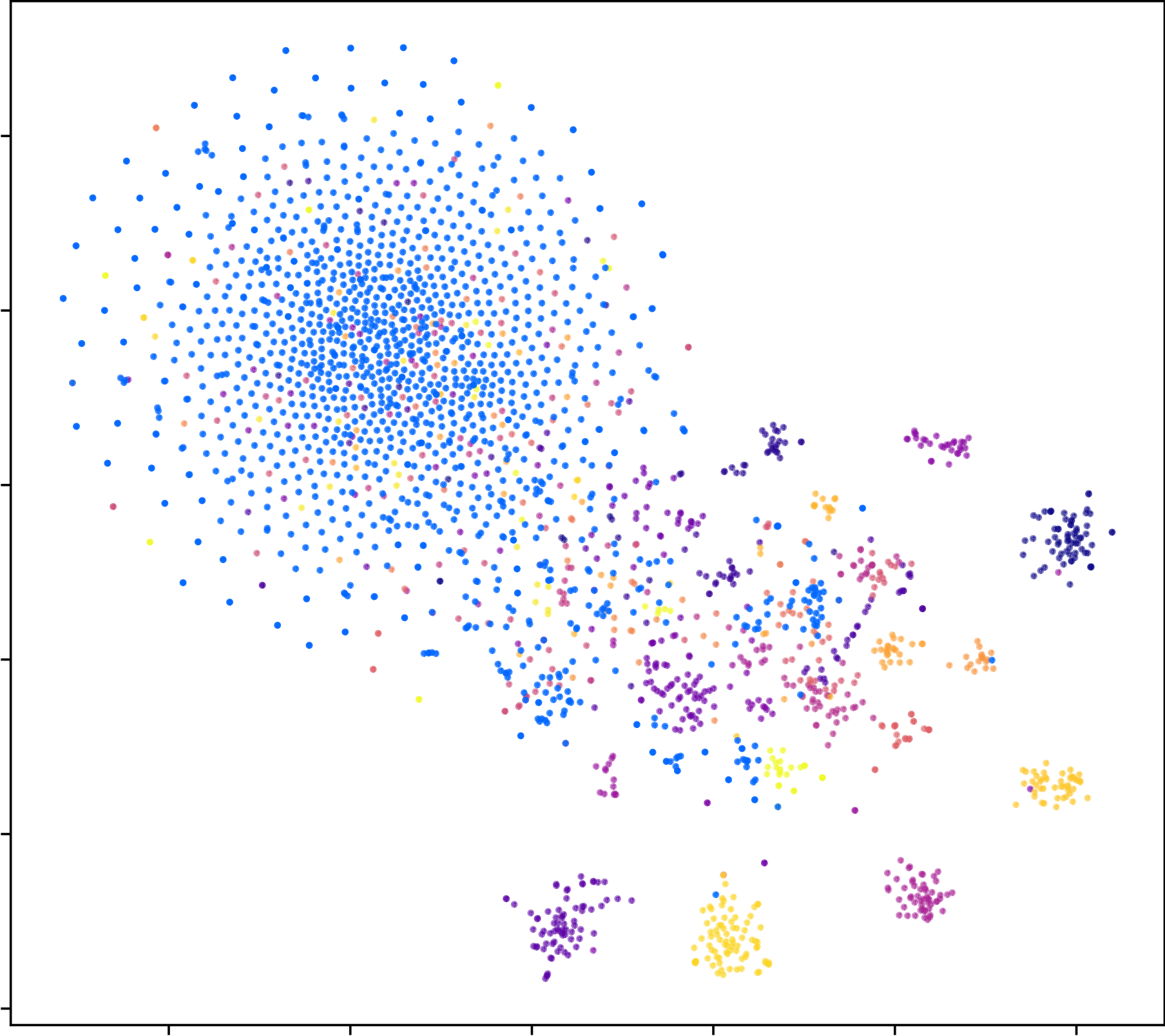
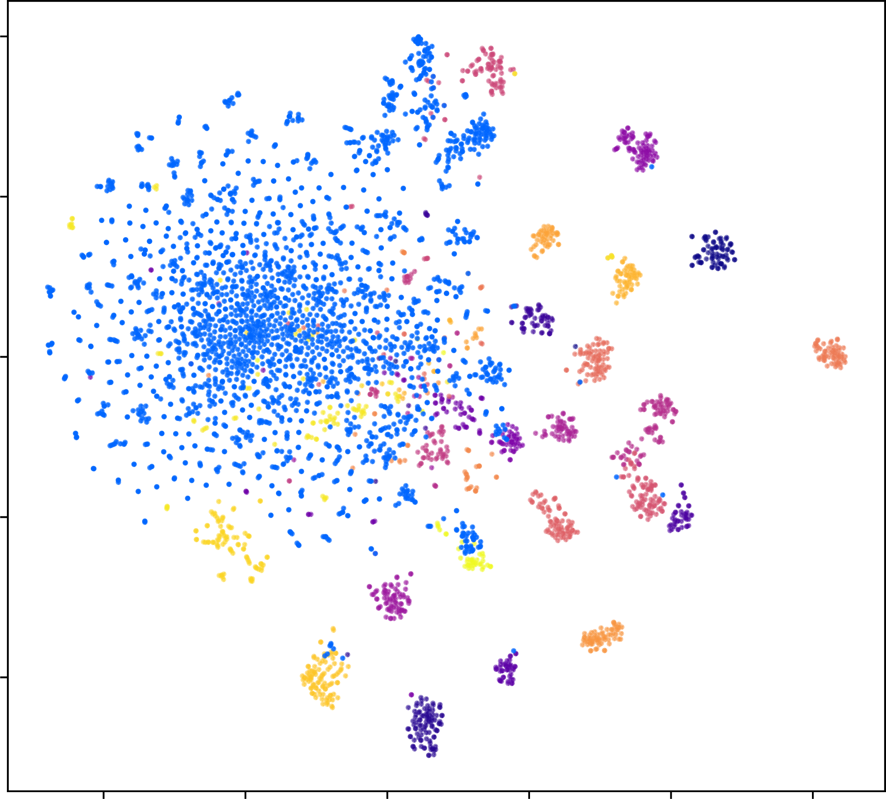
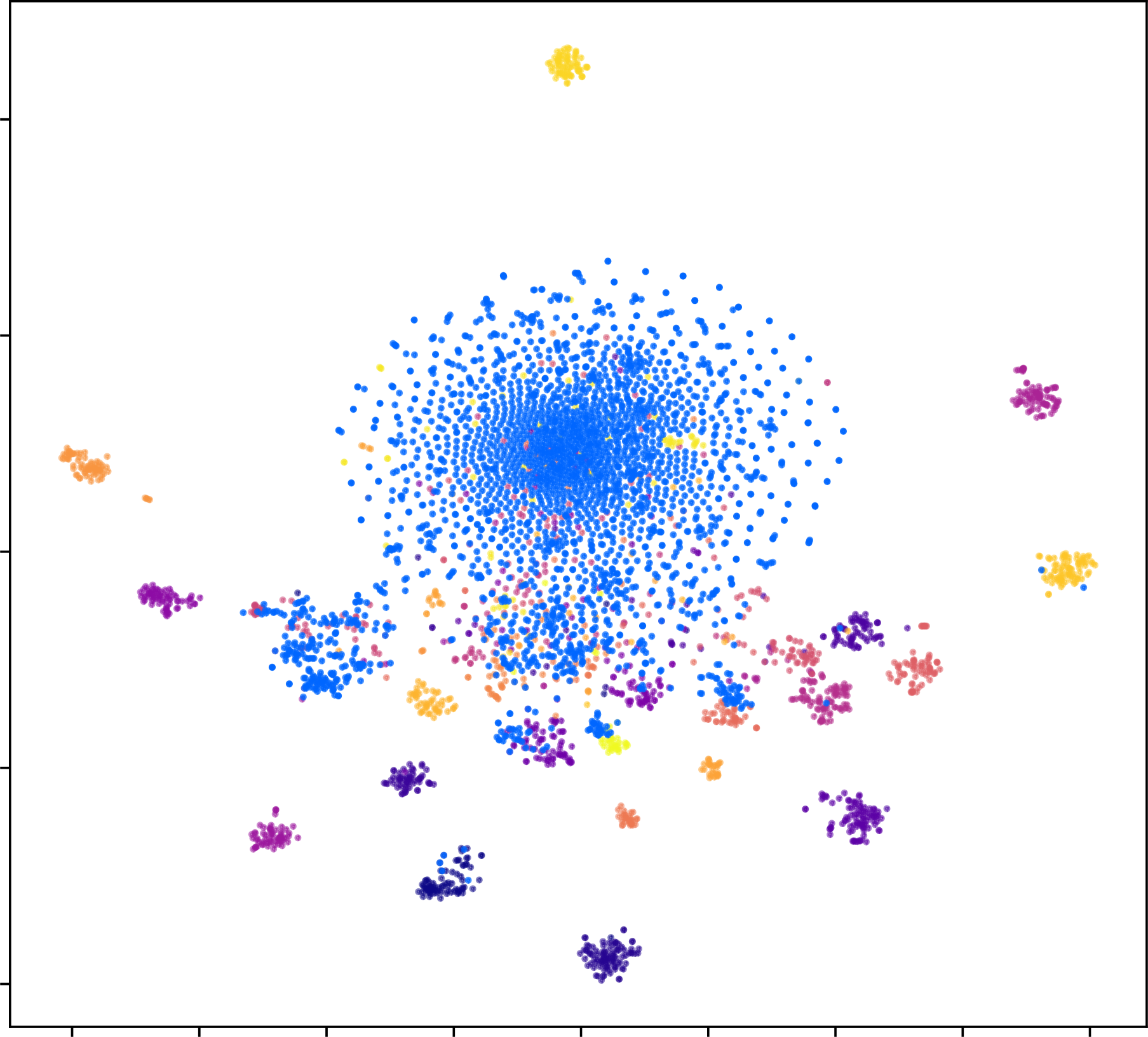
t-SNE Visualization. We perform t-SNE visualization of the raw CLIP features and the features filtered by the SUFF module across three domains of the Office-Home dataset, as shown in Figure 5. In the raw CLIP features, the image features of unknown and known classes are mixed within the same region. After filtering through the SUFF module, the unknown classes are significantly separated from the known class region while preserving the original separability of the known classes.
5 Conclusion
In this paper, we propose a novel CLIPXpert model to address two critical limitations in CLIP-based SF-OSDA: the reliance on suboptimal fixed thresholds and the neglect of the intrinsic tendency of unknown classes toward known classes. The BGAT module dynamically optimizes thresholds by modeling sample score distributions to balance known-class recognition and unknown sample detection, while SUFF mitigates this tendency through feature filtering to improve their separability. Extensive experiments demonstrate that CLIPXpert achieves performance comparable to that of state-of-the-art trained approaches without source data or extra training. These results also validate that proper exploitation of CLIP’s zero-shot potential, coupled with lightweight statistical adaptation, can advance SF-OSDA without costly training interventions. Our work can establish a new paradigm for efficient open-set domain adaptation in resource-constrained scenarios.
References
- Bishop and Nasrabadi [2006] Christopher M Bishop and Nasser M Nasrabadi. Pattern recognition and machine learning. Springer, 2006.
- Bossard et al. [2014] Lukas Bossard, Matthieu Guillaumin, and Luc Van Gool. Food-101–mining discriminative components with random forests. In Computer vision–ECCV 2014: 13th European conference, zurich, Switzerland, September 6-12, 2014, proceedings, part VI 13, pages 446–461. Springer, 2014.
- Box and Cox [1964] George EP Box and David R Cox. An analysis of transformations. Journal of the Royal Statistical Society Series B: Statistical Methodology, 26(2):211–243, 1964.
- Bucci et al. [2020] Silvia Bucci, Mohammad Reza Loghmani, and Tatiana Tommasi. On the effectiveness of image rotation for open set domain adaptation. In European conference on computer vision, pages 422–438. Springer, 2020.
- Chang et al. [2024] Kaiyan Chang, Songcheng Xu, Chenglong Wang, Yingfeng Luo, Xiaoqian Liu, Tong Xiao, and Jingbo Zhu. Efficient prompting methods for large language models: A survey. arXiv preprint arXiv:2404.01077, 2024.
- Cimpoi et al. [2014] Mircea Cimpoi, Subhransu Maji, Iasonas Kokkinos, Sammy Mohamed, and Andrea Vedaldi. Describing textures in the wild. In Proceedings of the IEEE conference on computer vision and pattern recognition, pages 3606–3613, 2014.
- Dempster et al. [1977] Arthur P Dempster, Nan M Laird, and Donald B Rubin. Maximum likelihood from incomplete data via the em algorithm. Journal of the royal statistical society: series B (methodological), 39(1):1–22, 1977.
- Deng et al. [2009] Jia Deng, Wei Dong, Richard Socher, Li-Jia Li, Kai Li, and Li Fei-Fei. Imagenet: A large-scale hierarchical image database. In 2009 IEEE conference on computer vision and pattern recognition, pages 248–255. Ieee, 2009.
- Eckart and Young [1936] Carl Eckart and Gale Young. The approximation of one matrix by another of lower rank. Psychometrika, 1(3):211–218, 1936.
- Fei-Fei et al. [2004] Li Fei-Fei, Rob Fergus, and Pietro Perona. Learning generative visual models from few training examples: An incremental bayesian approach tested on 101 object categories. In 2004 conference on computer vision and pattern recognition workshop, pages 178–178. IEEE, 2004.
- Fisher [1921] Ronald A Fisher. On the” probable error” of a coefficient of correlation deduced from a small sample. Metron, 1:3–32, 1921.
- Garg et al. [2022] Saurabh Garg, Sivaraman Balakrishnan, and Zachary Lipton. Domain adaptation under open set label shift. Advances in Neural Information Processing Systems, 35:22531–22546, 2022.
- Han et al. [2022] Kai Han, Yunhe Wang, Hanting Chen, Xinghao Chen, Jianyuan Guo, Zhenhua Liu, Yehui Tang, An Xiao, Chunjing Xu, Yixing Xu, et al. A survey on vision transformer. IEEE transactions on pattern analysis and machine intelligence, 45(1):87–110, 2022.
- He et al. [2016] Kaiming He, Xiangyu Zhang, Shaoqing Ren, and Jian Sun. Deep residual learning for image recognition. In Proceedings of the IEEE conference on computer vision and pattern recognition, pages 770–778, 2016.
- Helber et al. [2019] Patrick Helber, Benjamin Bischke, Andreas Dengel, and Damian Borth. Eurosat: A novel dataset and deep learning benchmark for land use and land cover classification. IEEE Journal of Selected Topics in Applied Earth Observations and Remote Sensing, 12(7):2217–2226, 2019.
- Hendrycks and Gimpel [2016] Dan Hendrycks and Kevin Gimpel. A baseline for detecting misclassified and out-of-distribution examples in neural networks. arXiv preprint arXiv:1610.02136, 2016.
- Jahan and Savakis [2024] Chowdhury Sadman Jahan and Andreas Savakis. Unknown sample discovery for source free open set domain adaptation. In Proceedings of the IEEE/CVF Conference on Computer Vision and Pattern Recognition, pages 1067–1076, 2024.
- Khattak et al. [2023] Muhammad Uzair Khattak, Hanoona Rasheed, Muhammad Maaz, Salman Khan, and Fahad Shahbaz Khan. Maple: Multi-modal prompt learning. In Proceedings of the IEEE/CVF conference on computer vision and pattern recognition, pages 19113–19122, 2023.
- Krause et al. [2013] Jonathan Krause, Michael Stark, Jia Deng, and Li Fei-Fei. 3d object representations for fine-grained categorization. In Proceedings of the IEEE international conference on computer vision workshops, pages 554–561, 2013.
- Lai et al. [2023] Zhengfeng Lai, Noranart Vesdapunt, Ning Zhou, Jun Wu, Cong Phuoc Huynh, Xuelu Li, Kah Kuen Fu, and Chen-Nee Chuah. Padclip: Pseudo-labeling with adaptive debiasing in clip for unsupervised domain adaptation. In Proceedings of the IEEE/CVF International Conference on Computer Vision, pages 16155–16165, 2023.
- Li et al. [2023] Wuyang Li, Jie Liu, Bo Han, and Yixuan Yuan. Adjustment and alignment for unbiased open set domain adaptation. In Proceedings of the IEEE/CVF Conference on Computer Vision and Pattern Recognition, pages 24110–24119, 2023.
- Li et al. [2024] Xinyao Li, Yuke Li, Zhekai Du, Fengling Li, Ke Lu, and Jingjing Li. Split to merge: Unifying separated modalities for unsupervised domain adaptation. In Proceedings of the IEEE/CVF Conference on Computer Vision and Pattern Recognition, pages 23364–23374, 2024.
- Liang et al. [2020] Jian Liang, Dapeng Hu, and Jiashi Feng. Do we really need to access the source data? source hypothesis transfer for unsupervised domain adaptation. In International conference on machine learning, pages 6028–6039. PMLR, 2020.
- Liang et al. [2021] Jian Liang, Dapeng Hu, Jiashi Feng, and Ran He. Umad: Universal model adaptation under domain and category shift. arXiv preprint arXiv:2112.08553, 2021.
- Liang et al. [2024] Jian Liang, Lijun Sheng, Zhengbo Wang, Ran He, and Tieniu Tan. Realistic unsupervised clip fine-tuning with universal entropy optimization. In Proceedings of the 41st International Conference on Machine Learning, pages 29667–29681, 2024.
- Liu et al. [2019] Hong Liu, Zhangjie Cao, Mingsheng Long, Jianmin Wang, and Qiang Yang. Separate to adapt: Open set domain adaptation via progressive separation. In Proceedings of the IEEE/CVF conference on computer vision and pattern recognition, pages 2927–2936, 2019.
- Liu et al. [2020] Weitang Liu, Xiaoyun Wang, John Owens, and Yixuan Li. Energy-based out-of-distribution detection. Advances in neural information processing systems, 33:21464–21475, 2020.
- Luo et al. [2020] Yadan Luo, Zijian Wang, Zi Huang, and Mahsa Baktashmotlagh. Progressive graph learning for open-set domain adaptation. In International Conference on Machine Learning, pages 6468–6478. PMLR, 2020.
- Luo et al. [2023] Yadan Luo, Zijian Wang, Zhuoxiao Chen, Zi Huang, and Mahsa Baktashmotlagh. Source-free progressive graph learning for open-set domain adaptation. IEEE Transactions on Pattern Analysis and Machine Intelligence, 45(9):11240–11255, 2023.
- Min et al. [2023] Youngjo Min, Kwangrok Ryoo, Bumsoo Kim, and Taesup Kim. Uota: Unsupervised open-set task adaptation using a vision-language foundation model. In Workshop on Efficient Systems for Foundation Models@ ICML2023, 2023.
- Ming et al. [2022] Yifei Ming, Ziyang Cai, Jiuxiang Gu, Yiyou Sun, Wei Li, and Yixuan Li. Delving into out-of-distribution detection with vision-language representations. Advances in neural information processing systems, 35:35087–35102, 2022.
- Monga et al. [2024] Munish Monga, Sachin Kumar Giroh, Ankit Jha, Mainak Singha, Biplab Banerjee, and Jocelyn Chanussot. Cosmo: Clip talks on open-set multi-target domain adaptation. In 35th British Machine Vision Conference 2024, BMVC 2024, Glasgow, UK, November 25-28, 2024. BMVA, 2024.
- Nilsback and Zisserman [2008] Maria-Elena Nilsback and Andrew Zisserman. Automated flower classification over a large number of classes. In 2008 Sixth Indian conference on computer vision, graphics & image processing, pages 722–729. IEEE, 2008.
- Panareda Busto and Gall [2017] Pau Panareda Busto and Juergen Gall. Open set domain adaptation. In Proceedings of the IEEE international conference on computer vision, pages 754–763, 2017.
- Parkhi et al. [2012] Omkar M Parkhi, Andrea Vedaldi, Andrew Zisserman, and CV Jawahar. Cats and dogs. In 2012 IEEE conference on computer vision and pattern recognition, pages 3498–3505. IEEE, 2012.
- Peng et al. [2017] Xingchao Peng, Ben Usman, Neela Kaushik, Judy Hoffman, Dequan Wang, and Kate Saenko. Visda: The visual domain adaptation challenge. arXiv preprint arXiv:1710.06924, 2017.
- Peng et al. [2019] Xingchao Peng, Qinxun Bai, Xide Xia, Zijun Huang, Kate Saenko, and Bo Wang. Moment matching for multi-source domain adaptation. In Proceedings of the IEEE/CVF international conference on computer vision, pages 1406–1415, 2019.
- Platt [1998] John Platt. Sequential minimal optimization: A fast algorithm for training support vector machines. 1998.
- Qu et al. [2023] Sanqing Qu, Tianpei Zou, Florian Röhrbein, Cewu Lu, Guang Chen, Dacheng Tao, and Changjun Jiang. Upcycling models under domain and category shift. In Proceedings of the IEEE/CVF conference on computer vision and pattern recognition, pages 20019–20028, 2023.
- Qu et al. [2024] Sanqing Qu, Tianpei Zou, Lianghua He, Florian Röhrbein, Alois Knoll, Guang Chen, and Changjun Jiang. Lead: Learning decomposition for source-free universal domain adaptation. In Proceedings of the IEEE/CVF Conference on Computer Vision and Pattern Recognition, pages 23334–23343, 2024.
- Radford et al. [2021] Alec Radford, Jong Wook Kim, Chris Hallacy, Aditya Ramesh, Gabriel Goh, Sandhini Agarwal, Girish Sastry, Amanda Askell, Pamela Mishkin, Jack Clark, et al. Learning transferable visual models from natural language supervision. In International conference on machine learning, pages 8748–8763. PmLR, 2021.
- Shao et al. [2024] Shuai Shao, Yu Bai, Yan Wang, Baodi Liu, and Yicong Zhou. Deil: Direct-and-inverse clip for open-world few-shot learning. In Proceedings of the IEEE/CVF Conference on Computer Vision and Pattern Recognition, pages 28505–28514, 2024.
- Shi et al. [2024] Bowen Shi, Peisen Zhao, Zichen Wang, Yuhang Zhang, Yaoming Wang, Jin Li, Wenrui Dai, Junni Zou, Hongkai Xiong, Qi Tian, et al. Umg-clip: a unified multi-granularity vision generalist for open-world understanding. In European Conference on Computer Vision, pages 259–277. Springer, 2024.
- Singha et al. [2023] Mainak Singha, Harsh Pal, Ankit Jha, and Biplab Banerjee. Ad-clip: Adapting domains in prompt space using clip. In Proceedings of the IEEE/CVF International Conference on Computer Vision, pages 4355–4364, 2023.
- Venkateswara et al. [2017] Hemanth Venkateswara, Jose Eusebio, Shayok Chakraborty, and Sethuraman Panchanathan. Deep hashing network for unsupervised domain adaptation. In Proceedings of the IEEE conference on computer vision and pattern recognition, pages 5018–5027, 2017.
- Wu et al. [2024] Jianzong Wu, Xiangtai Li, Shilin Xu, Haobo Yuan, Henghui Ding, Yibo Yang, Xia Li, Jiangning Zhang, Yunhai Tong, Xudong Jiang, et al. Towards open vocabulary learning: A survey. IEEE Transactions on Pattern Analysis and Machine Intelligence, 46(7):5092–5113, 2024.
- Xiao et al. [2010] Jianxiong Xiao, James Hays, Krista A Ehinger, Aude Oliva, and Antonio Torralba. Sun database: Large-scale scene recognition from abbey to zoo. In 2010 IEEE computer society conference on computer vision and pattern recognition, pages 3485–3492. IEEE, 2010.
- Yu et al. [2025] Qing Yu, Go Irie, and Kiyoharu Aizawa. Open-set domain adaptation with visual-language foundation models. Computer Vision and Image Understanding, 250:104230, 2025.
- Zhang et al. [2024a] Jingyi Zhang, Jiaxing Huang, Sheng Jin, and Shijian Lu. Vision-language models for vision tasks: A survey. IEEE Transactions on Pattern Analysis and Machine Intelligence, 2024a.
- Zhang et al. [2024b] Wenyu Zhang, Li Shen, and Chuan-Sheng Foo. Source-free domain adaptation guided by vision and vision-language pre-training. International Journal of Computer Vision, pages 1–23, 2024b.
- Zhou et al. [2022a] Kaiyang Zhou, Jingkang Yang, Chen Change Loy, and Ziwei Liu. Conditional prompt learning for vision-language models. In Proceedings of the IEEE/CVF conference on computer vision and pattern recognition, pages 16816–16825, 2022a.
- Zhou et al. [2022b] Kaiyang Zhou, Jingkang Yang, Chen Change Loy, and Ziwei Liu. Learning to prompt for vision-language models. International Journal of Computer Vision, 130(9):2337–2348, 2022b.
Appendix A Proof
Theorem 1:
Let the known class follow a Gaussian distribution and the unknown class follow a Gaussian distribution , where . Define the total classification error area as:
where and denote the probability density functions (PDFs) of the two distributions. Then, the optimal threshold that minimizes satisfies:
i.e., is the x-coordinate of the intersection point of the two Gaussian PDFs.
Proof:
1. Construction of the Error Function
The total classification error consists of two components:
(1) The first term : the probability that an unknown sample is misclassified as a known sample (false negative)
(2) The second term : the probability that a known sample is misclassified as an unknown sample (false positive).
2. Condition for Extremum
Taking the derivative of with respect to , we obtain:
Setting the derivative to zero to find the critical point:
3. econd Derivative Test
Computing the second derivative:
At the intersection point : When , we have (since is increasing on the right) and (since is decreasing on the right). Consequently, , confirming that is a minimum.
Conclusion : Under the assumption of bimodal Gaussian distributions, the optimal threshold that minimizes the total classification error corresponds to the x-coordinate of the intersection of the two probability density functions. This result holds for any combination of variances and does not require prior probability assumptions.
Theorem 2:
Let the known class follow and the unknown class follow , with probability density functions (PDFs) defined as:
Step 1: Intersection Equation
The intersection of the two distributions satisfies . Simplifying this equality yields:
Step 2: Implicit Function Differentiation
Treating Equation (1) as an implicit function , we apply the implicit function theorem to compute :
where the partial derivatives are:
Step 3: Sensitivity Analysis
As : (1) The dominant term in is .
(2) The dominant term in is .
Thus,
Conclusion : When is extremely small, the magnitude of scales as . Even if is near (i.e., the intersection point is close to the known class mean), this derivative remains significant. This demonstrates that the intersection coordinate is highly sensitive to infinitesimal changes in . The sensitivity arises from the amplification effect caused by the cubic () and quadratic () terms of in the denominators of the partial derivatives.
| Setting | ImageNet | Caltech101 | DTD | EuroSAT | Food101 | Flowers102 | OxfordPets | SUN397 | StanfordCars | UCF101 | Office-Home | VisDA-2017 | DomainNet |
|---|---|---|---|---|---|---|---|---|---|---|---|---|---|
| 200 | 35 | 15 | 5 | 35 | 65 | 15 | 100 | 80 | 25 | 25 | 6 | 100 | |
| 800 | 66 | 22 | 5 | 66 | 37 | 22 | 297 | 116 | 76 | 40 | 6 | 245 |
| Method | Score | threshold | ImageNet | Caltech101 | DTD | Food101 | OxfordPets | SUN397 | OfficeHome | VisDA2017 | AVG |
|---|---|---|---|---|---|---|---|---|---|---|---|
| CLIP + SUFF | MCM | fixed | 60.81 | 89.51 | 60.66 | 84.55 | 69.44 | 67.79 | 80.32 | 84.03 | 74.64 |
| mean | 68.97 | 88.39 | 62.19 | 83.38 | 72.80 | 70.78 | 80.09 | 86.19 | 76.60 | ||
| BGAT | 69.91 | 89.53 | 61.49 | 85.1 | 74.78 | 70.74 | 80.68 | 87.29 | 77.44 | ||
| Entropy | fixed | 64.73 | 89.55 | 56.32 | 86.67 | 75.81 | 70.02 | 80.90 | 87.26 | 76.41 | |
| mean | 68.97 | 89.54 | 61.29 | 84.67 | 76.07 | 70.12 | 80.95 | 87.18 | 77.35 | ||
| BGAT | 71.97 | 89.84 | 62.17 | 86.64 | 77.61 | 70.81 | 81.16 | 87.17 | 78.42 | ||
| VAR | fixed | 41.76 | 90.27 | 53.19 | 83.70 | 75.47 | 55.94 | 79.87 | 87.31 | 70.94 | |
| mean | 66.96 | 90.15 | 61.61 | 85.09 | 75.29 | 69.85 | 80.57 | 87.17 | 77.09 | ||
| BGAT | 70.32 | 90.86 | 61.72 | 85.53 | 75.48 | 71.17 | 80.30 | 87.15 | 77.82 | ||
| CLIP | MCM | fixed | 60.42 | 74.30 | 59.88 | 57.43 | 27.67 | 59.72 | 56.89 | 52.73 | 56.13 |
| mean | 61.51 | 82.04 | 59.87 | 74.64 | 65.81 | 65.23 | 73.65 | 80.52 | 70.41 | ||
| BGAT | 62.33 | 85.74 | 60.72 | 80.95 | 70.56 | 66.68 | 78.41 | 86.38 | 73.97 | ||
| Entropy | fixed | 61.60 | 73.91 | 60.53 | 48.76 | 17.90 | 53.24 | 55.27 | 72.43 | 55.46 | |
| mean | 61.51 | 84.07 | 60.64 | 76.64 | 69.69 | 65.67 | 75.49 | 83.14 | 72.11 | ||
| BGAT | 63.25 | 87.83 | 61.29 | 81.03 | 70.84 | 67.95 | 78.26 | 86.09 | 74.57 | ||
| VAR | fixed | 57.73 | 85.7 | 57.05 | 76.39 | 59.07 | 66.61 | 73.11 | 77.91 | 69.20 | |
| mean | 63.08 | 85.31 | 61.18 | 77.99 | 68.73 | 67.50 | 76.20 | 83.44 | 72.93 | ||
| BGAT | 63.10 | 86.11 | 60.17 | 81.16 | 70.66 | 66.85 | 78.39 | 86.30 | 74.09 |
Appendix B Experiments
B.1 Datasets
To comprehensively evaluate the effectiveness of the proposed method, we conduct extensive experimental validation on multiple public datasets. Given that our method does not require source domain data, we first test it on four widely used open-set domain adaptation (OSDA) benchmark datasets: Office-Home [45] (65 categories, 4 domains), VisDA-2017 [36] (12 categories, cross-domain adaptation from synthetic to real-world scenes), DomainNet [37] (345 categories, 6 domains). Furthermore, to further assess the generalization ability of our method, we select 10 publicly available datasets from the Visual task Adaptation Benchmark (VATB) for experimentation, including ImageNet [8], Caltech101 [10], EuroSAT [15], Food101 [2], Flowers102 [33], OxfordPets [35], SUN397 [47], StandfordCars [19] and DTD [6]. These datasets cover diverse visual tasks, ranging from fine-grained classification to scene recognition, with characteristics such as large category numbers (100-1000 categories), large data scales (tens of thousands to millions of samples), and significant domain differences, providing a comprehensive testing platform for evaluating open-set domain adaptation methods.
In the experiments, the selection criteria for known classes in the four OSDA datasets followed the UOTA [30] setting to ensure comparability and consistency. For the remaining 10 VATB datasets, we test with varying proportions of unknown classes to enhance the generality and robustness of the experiments, with the specific division of known and unknown classes for each dataset shown in Table 5. Specifically, we sort the class names of each dataset in dictionary order, assigning the first classes as known classes, while the rest are considered unknown classes. This diversified testing setup not only validates the adaptability of the method across different data distributions but also comprehensively evaluates its performance on open-set domain adaptation tasks. Additionally, it should be noted that for the 10 VATB datasets, we directly conduct testing on the test set and evaluate performance. The test set partitioning follows the approach of CoOp[52].
| Score | SUFF | ImageNet | Caltech101 | DTD | Food101 | OxfordPets | SUN397 | OfficeHome | VisDa2017 | AVG |
|---|---|---|---|---|---|---|---|---|---|---|
| Entropy | 63.25 | 87.83 | 61.29 | 81.03 | 70.84 | 67.95 | 78.26 | 86.09 | 74.57 | |
| 71.97 | 89.84 | 62.17 | 86.64 | 77.61 | 70.81 | 81.16 | 87.17 | 78.42 | ||
| MCM | 62.33 | 85.74 | 60.72 | 80.95 | 70.56 | 66.68 | 78.41 | 86.38 | 73.97 | |
| 69.91 | 89.53 | 61.49 | 85.1 | 74.78 | 70.74 | 80.68 | 87.29 | 77.44 | ||
| VAR | 63.1 | 86.11 | 60.17 | 81.16 | 70.66 | 66.85 | 78.39 | 86.3 | 74.09 | |
| 70.32 | 90.86 | 61.72 | 85.53 | 75.48 | 71.17 | 80.30 | 87.15 | 77.82 |
| Method | Threshold | ImageNet | Caltech101 | DTD | EuroSAT | Food101 | Flowres102 | OxfordPets | SUN397 | StandfordCars | UCF101 | AVG |
|---|---|---|---|---|---|---|---|---|---|---|---|---|
| UEO | fixed | 58.56 | 70.02 | 36.55 | 36.05 | 49.56 | 52.14 | 40.34 | 47.97 | 41.85 | 58.4 | 49.14 |
| mean | 59.54 | 80.06 | 42.31 | 36.51 | 72.56 | 63.39 | 65.47 | 59.77 | 50.91 | 65.18 | 59.57 | |
| BGAT | 60.14 | 84.15 | 42.31 | 36.33 | 79.56 | 63.8 | 69.32 | 62 | 50.08 | 67.82 | 61.55 | |
| BGAT + SUFF | 66.27 | 86.7 | 39.8 | 37.9 | 83.07 | 65.17 | 73.31 | 66.2 | 49.19 | 71.04 | 63.87 |
| Threshold type | Art | Clipart | Product | Real_world | AVG |
|---|---|---|---|---|---|
| fixed | 55.36 | 50.73 | 36.31 | 40.08 | 45.62 |
| mean | 70.84 | 65.23 | 72.04 | 74.68 | 70.70 |
| BGAT | 69.38 | 69.81 | 78.64 | 79.27 | 74.28 |
| BGAT + SUFF | 72.19 | 73.28 | 83.7 | 82.32 | 77.87 |
B.2 Baselines
To the best of our knowledge, the proposed Source-Free open-set domain adaptation (SF-OSDA) method, which requires neither source domain data nor training, has not been explored in existing research. Therefore, we select the following three categories of baseline methods for comparison to ensure the comprehensiveness and fairness of the evaluation:
-
•
CLIP-zero shot-based sample scoring and threshold selection methods: For a fair comparison, we evaluate three different scoring mechanisms: Maximum Concept Matching(MCM) [31], Entropy [16], and Variance. We also test two threshold selection strategies: the commonly used fixed threshold (MAX/2) and a dynamic average threshold based on target dataset statistical properties to ensure the validity of the evaluation.
-
•
OSDA methods that directly involve source domain data in target domain training or rely on source domain pre-trained models: These include ANNA [21], USD [17], LAED [40], SHOT [23], UMAD [24], Co-learn++ [50], DIFO, Cosmo [32], and ODAwVL [48]. Among these, Co-learn++, DIFO, Cosmo, and ODAwVL leverage the CLIP model, while the others are based on ImageNet pre-trained single-modal models. These methods represent typical implementations of traditional OSDA approaches.
-
•
Methods for unsupervised training and unknown class detection directly on the unlabeled target domain: These include UOTA [30] and UEO [25]. These methods do not require source domain data and perform model optimization and unknown class identification directly on the target domain, making them closest to the setting of our proposed method.
Through the comparison of these three categories of baseline methods, we can comprehensively assess the performance of the proposed method in different scenarios and validate its unique advantages in the absence of source domain data and training conditions.
In this paper, to facilitate performance comparison with other OSDA methods, we use the commonly adopted HOS metric, which is the harmonic mean of the average accuracy for known classes and the accuracy for unknown classes. The calculation formula is as follows:
| (17) |
Where represents the average accuracy of known classes, and denotes the accuracy of unknown class recognition. This metric reflects the overall performance of the model on both known and unknown classes, balancing the recognition ability for known classes and the detection ability for unknown classes. Therefore, HOS provides an effective standard for evaluating OSDA methods.
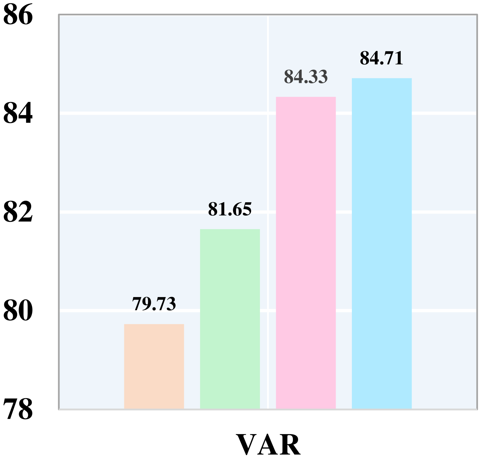
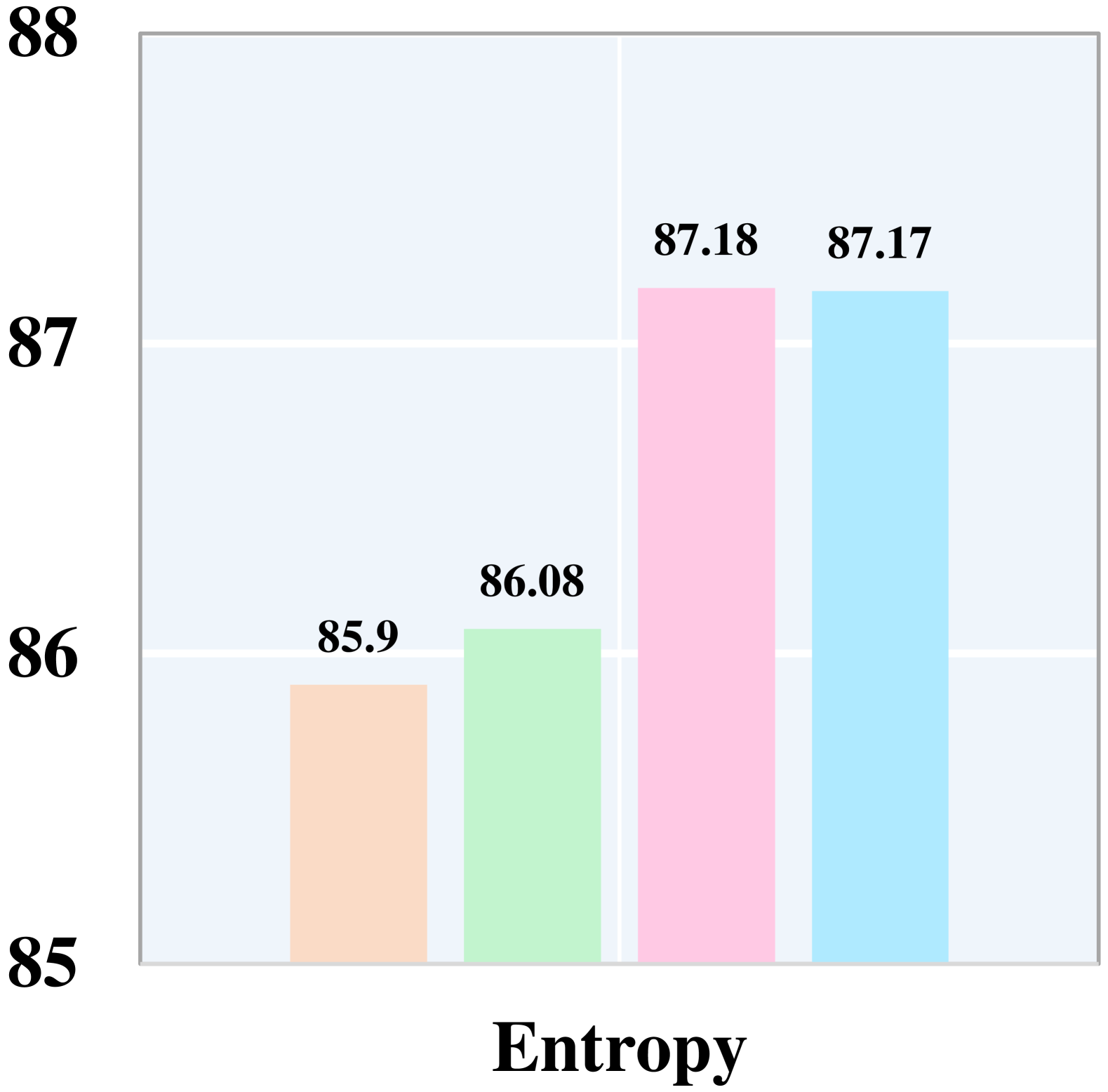
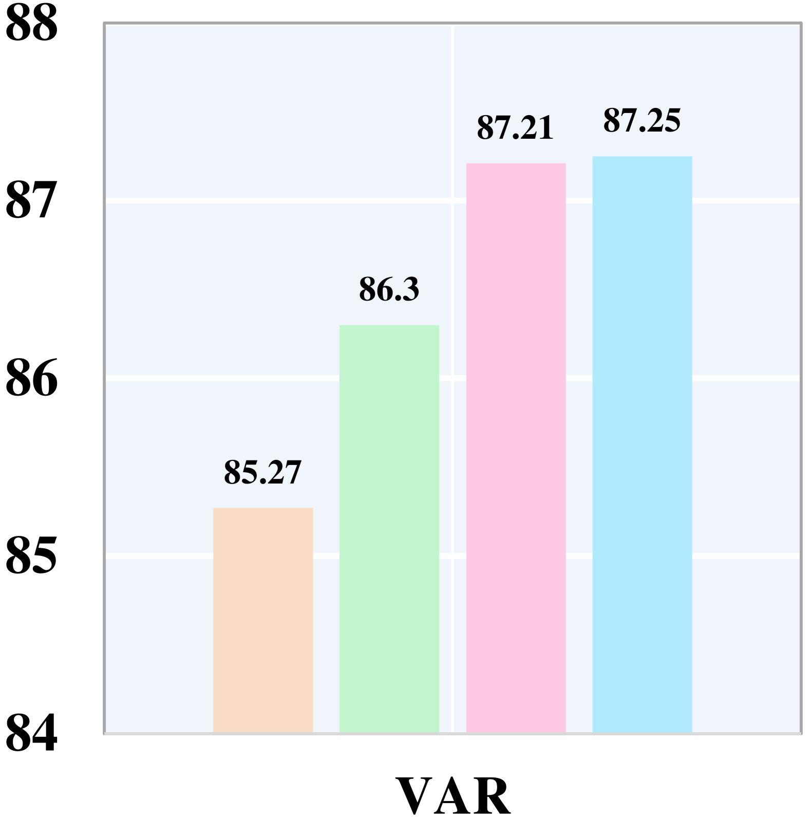
| Score | Box-Cox | Art | Clipart | Product | Real World | AVG |
|---|---|---|---|---|---|---|
| Entropy | 85.29 | 79.71 | 84.6 | 87.91 | 84.38 | |
| 84.76 | 79.42 | 87.01 | 89.89 | 85.27 | ||
| MCM | 84.84 | 79.29 | 80.67 | 86.3 | 82.78 | |
| 85 | 79.88 | 84.55 | 87.99 | 84.36 | ||
| VAR | 86.97 | 80.09 | 83.28 | 86.97 | 84.33 | |
| 85.1 | 80.31 | 85.12 | 88.29 | 84.71 |
| Method | Score type | Box-Cox | ImageNet | Caltech101 | DTD | EuroSAT | Food101 | Flowres102 | OxfordPets | SUN397 | StandfordCars | UCF101 | VisDA-2017 | AVG |
|---|---|---|---|---|---|---|---|---|---|---|---|---|---|---|
| CLIP | MCM | 62.24 | 85.30 | 60.68 | 51.70 | 79.52 | 67.40 | 69.18 | 66.67 | 50.67 | 71.69 | 83.40 | 68.04 | |
| 62.33 | 85.74 | 60.72 | 51.48 | 80.95 | 66.32 | 70.56 | 66.68 | 50.51 | 71.51 | 86.38 | 68.47 | |||
| Entropy | 62.42 | 87.96 | 60.29 | 52.03 | 81.72 | 66.85 | 70.91 | 66.28 | 53.82 | 72.74 | 85.90 | 69.17 | ||
| 63.25 | 87.83 | 61.29 | 52.10 | 81.03 | 68.35 | 70.84 | 67.95 | 54.05 | 74.26 | 86.09 | 69.73 | |||
| VAR | 63.13 | 86.15 | 60.05 | 51.58 | 80.05 | 67.31 | 70.15 | 67.34 | 50.17 | 71.89 | 85.27 | 68.46 | ||
| 63.10 | 86.11 | 60.17 | 51.62 | 81.16 | 64.75 | 70.66 | 66.85 | 48.91 | 71.22 | 86.30 | 68.26 | |||
| CLIP+SUFF | MCM | 69.31 | 88.95 | 61.55 | 51.41 | 84.96 | 67.47 | 74.22 | 70.72 | 51.15 | 74.28 | 86.91 | 70.99 | |
| 69.91 | 89.53 | 61.49 | 51.41 | 85.10 | 65.70 | 74.78 | 70.74 | 51.53 | 73.91 | 87.29 | 71.04 | |||
| Entropy | 71.88 | 90.36 | 59.43 | 51.83 | 86.46 | 69.56 | 76.94 | 70.82 | 55.81 | 74.32 | 87.19 | 72.24 | ||
| 71.97 | 89.84 | 62.17 | 51.84 | 86.64 | 68.88 | 77.61 | 70.81 | 55.61 | 76.22 | 87.17 | 72.61 | |||
| VAR | 54.34 | 90.45 | 58.65 | 51.63 | 85.57 | 66.20 | 75.39 | 65.27 | 46.76 | 77.08 | 87.21 | 68.96 | ||
| 70.32 | 90.86 | 61.72 | 51.63 | 85.53 | 65.37 | 75.48 | 71.17 | 54.91 | 76.17 | 87.15 | 71.85 |

B.3 Ablation Study
This section provides additional experiments not detailed in the main text’s ablation study, including the exact numerical values of some tables and figures, as well as ablation experiments omitted due to space constraints. A more comprehensive dataset and ablation results are presented in this subsection.
Effectiveness of BGAT. As shown in Table 6, this table presents the detailed dataset corresponding to the six radar charts in Figure 3 of the main text. It can be observed that for the three sample scores computed from CLIP’s original features, using a fixed threshold (max/2) performs significantly worse than other methods. In contrast, using the mean value outperforms the fixed threshold by 14.28%, 16.65%, and 3.73% for the three sample scores, respectively. Furthermore, the threshold estimated by BGAT surpasses the mean-based method by 3.56%, 2.46%, and 4.89%, respectively, demonstrating the effectiveness of BGAT in threshold computation and fully enhancing CLIP’s performance in the SF-OSDA setting.
Additionally, after incorporating the SUFF module to filter out unknown class features, the model becomes slightly less sensitive to the threshold. However, the mean-based method still outperforms the fixed threshold, while BGAT continues to exceed the mean-based threshold method by 0.84%, 0.85%, and 0.73% across the three sample scores. This further highlights the robustness of BGAT.
Effectiveness of SUFF. As shown in Table 7, we validate the effectiveness of the proposed SUFF module on six VTAB datasets and two OSDA datasets. For Office-Home, we report the domain-averaged HOS, while for the other datasets, results are directly obtained from predictions on the corresponding test sets. It can be observed that the SUFF module significantly improves model performance across all three sample scores, with the largest improvement on ImageNet, reaching 8.72%, 7.58%, and 7.22%, respectively. On average across the eight datasets, SUFF achieves performance gains of 3.83%, 3.47%, and 3.73%, respectively.
Effectiveness of Box-Cox. We validate the effectiveness of Box-Cox on 12 datasets, with Office-Home containing four domains, while the other datasets are directly tested on their respective test sets. The detailed performance on the Office-Home dataset is shown in Table 10, where it is evident that the introduction of Box-Cox transformation improves model performance, with increases of 0.89%, 1.58%, and 0.38% across the three scores. Additionally, to further demonstrate the effectiveness of Box-Cox, the performance on the other 11 datasets is presented in Table 11. We also compare the impact of Box-Cox on the scores obtained from CLIP’s original features. Specifically, for the sample scores from CLIP’s original features, the introduction of Box-Cox results in an average improvement of 0.26%, while for the model with the SUFF module applied for feature filtering, Box-Cox leads to an average performance improvement of 1.1%.
Impact of BGAT and SUFF on UEO. We verify the impact of our proposed BGAT and SUFF modules on the trainable method UEO across 11 datasets. We compare the performance of the original UEO using three different threshold calculation methods: fixed threshold (max/2), target data average, and BGAT. Additionally, we evaluate the performance when using BGAT as the threshold calculation method and incorporating the SUFF module into UEO to fully validate the effectiveness of the two proposed modules. It is worth noting that due to the use of the soft prompt method from CoOp for fine-tuning in UEO, convergence is fast, but performance tends to decline in later stages of training. The best performance is often reached in the first epoch, as shown in Figure 6 6(b), so we conduct the comparison by validating after training for only one epoch.
As shown in Table 9, on the Office-Home dataset, the performance of the BGAT threshold surpasses the fixed threshold and average value threshold by 29.02% and 3.58%, respectively. After adding the SUFF module, the model performance further improves by 3.59%. For the 10 VATB datasets, as shown in Table 8, using BGAT as the threshold outperforms the fixed and average value thresholds by 12.41% and 1.98%, respectively. After incorporating the SUFF module, the model performance further improves by 2.32%.
B.4 Case Study
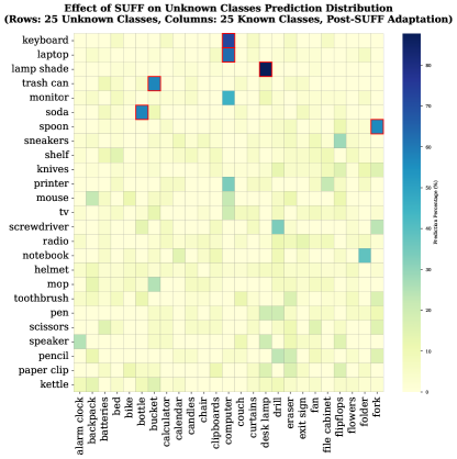
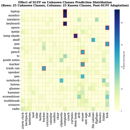
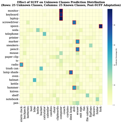
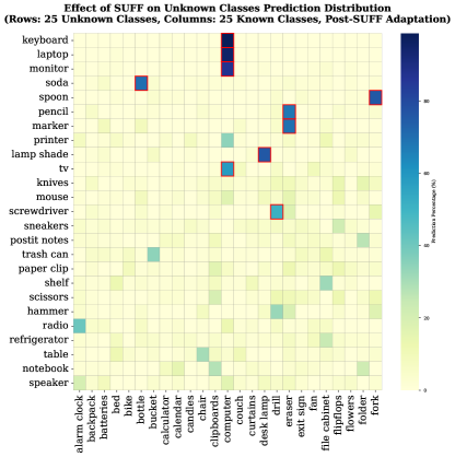
To analyze the tendency of removing certain unknown classes on the known classes, we visualize the distribution of the top 25 classes with the strongest tendency in the Office-Home dataset across four domains before and after filtering by the SUFF module. We also compare the change in entropy of all samples before and after filtering by the SUFF module.
As shown in Figure 8, each cell represents the distribution of predictions for all samples of an unknown class in one row, with each column indicating the distribution of unknown classes predicted as a specific known class. The darker the cell color, the more samples from the unknown class are classified into the corresponding known class. As shown in the first row of Table 8, it is evident that in the original CLIP predictions, many unknown classes exhibit a strong tendency toward known classes, causing these samples to have scores very close to known classes. This results in difficulty distinguishing these samples during unknown class detection. As shown in the second row of Table 8, after filtering by the SUFF module, the number of unknown classes with significant tendencies is notably reduced, allowing these hard-to-detect unknown class samples to be separated from the known classes.
Additionally, as shown in the first row of Table 9, the entropy of unknown classes computed from the original CLIP features is spread across different score ranges and significantly overlaps with that of the known classes. However, as shown in the second row of Table 9, after filtering by the SUFF module, the entropy of the unknown classes shifts significantly toward the maximum value, greatly enhancing the separability between known and unknown classes. Furthermore, it can be observed that the entropy of the known classes does not shift to the right during the feature filtering process, indicating that the SUFF module does not destroy the separability of known class features while filtering unknown class features.
Appendix C Algorithm Details and Pseudocode
In this section, we provide the detailed pseudocode of CLIPXpert. Our method aims to detect unknown samples and classify known-class samples in an unlabeled target dataset without requiring any source-domain data or additional training. The approach consists of the following key steps: (1) We leverage CLIP as an encoder to perform zero-shot classification, obtaining the initial classification results for known classes and computing sample scores based on these results. (2) The proposed BGAT module estimates the distribution of sample scores and derives the estimated mean scores for known and unknown classes, along with an initial threshold. (3) Based on these estimates, we perform an initial selection of samples and apply the proposed SUFF module to filter out unknown-class features. (4) We then recompute sample scores using the filtered features and re-estimate the final threshold via the BGAT module. (5) Finally, we classify all samples using the refined scores, the final threshold, and the initial classification results. The full procedure is detailed in Algorithm 1.
-
•
-
•
-
•
-
•
Execute steps 3, 4, and 5 again using to obtain the estimated final threshold .