Efficient state transition algorithm with guaranteed optimality

Abstract

As a constructivism-based intelligent optimization method, state transition algorithm (STA) has exhibited powerful search ability in optimization. However, the standard STA still shows slow convergence at a later stage for flat landscape and a user has to preset its maximum number of iterations (or function evaluations) by experience. To resolve these two issues, efficient state transition algorithm is proposed with guaranteed optimality. Firstly, novel translation transformations based on predictive modeling are proposed to generate more potential candidates by utilizing historical information. Secondly, parameter control strategies are proposed to accelerate the convergence. Thirdly, a specific termination condition is designed to guarantee that the STA can stop automatically at an optimal point, which is equivalent to the zero gradient in mathematical programming. Experimental results have demonstrated the effectiveness and superiority of the proposed method.

I Introduction

State transition algorithm (STA) is a novel intelligent optimization algorithm proposed in recent years [1, 2]. In STA, a solution to an optimization problem is considered as a state, and an update of a solution is considered as a state transition. Unlike the majority of swarm intelligence optimization algorithms based on imitation learning and behavioral cloning [3], the STA is inspired by constructivism-based learning [4]. That is to say, in STA, it just acquires the essential knowledge and constructs the necessary components, including globality, optimality, rapidity, convergence and controllability, aiming to find a global or near-global optimal solution as soon as possible. In standard STA [5], several state transformation operators are purposefully designed to generate candidate solutions. Specifically, the expansion transformation facilitates global search to ensure globality, while the rotation transformation supports local search to enhance optimality. Additionally, translation and axesion transformations are employed for heuristic search to improve rapidity. Furthermore, appropriate update strategies are implemented to ensure convergence. Moreover, each state transformation operator generates a regular neighborhood with an adjustable size, providing controllability. Due to its ease of understanding, convenience of use, as well as powerful search ability, it has found successfully applications in many practical engineering problems [6, 7, 8, 9, 10, 11].

As an intelligent optimization algorithm, besides generating new candidates and updating incumbents, the termination condition is also crucial component. In mathematical programming with continuously differentiable objective function, the widely used termination condition is the zero gradient, since it can guarantee the optimality due to Fermat’s theorem [12]. However, for the majority of existing intelligent optimization algorithms, it is not easy to propose an automatic termination condition to guarantee the optimality [13, 14, 15, 16, 17]. The simplest and most widely used termination condition in intelligent optimization algorithms is the maximum number of generations or iterations. However, this number is problem-dependent and has to be predefined by enough experience. If set too small, it may fail to find the optimal solution; conversely, if set too large, it may result in a waste of computing resources. What’s more, the maximum number of generations as stopping criterion is considered harmful, and how to set a good termination condition in intelligent optimization algorithms still remain open and need further require further exploration [18].

On the one hand, the standard STA faces the challenge of determining an appropriate termination condition as well. In standard STA, the maximum number of iterations (or function evaluations) is chosen as the termination condition, which should be preset and typically requires the expertise of an experienced user. Fortunately, the intrinsic characteristics in STA, especially the rotation transformation has the functionality of searching in a hypershere with a given radius, which makes it possible to set a specific termination condition that can guarantee the optimality automatically. On the other hand, the standard STA also shows slow convergence at a later stage. Several efforts have been made to address this issue. In [19], all state transformation factors are decreased periodically to enhance local exploitation in the later stages. In [1], an optimal parameter selection strategy was proposed to accelerate convergence; however, it requires some time to initiate the acceleration process. The question of how to incorporate appropriate mechanisms to accelerate convergence in STA requires further investigation.

To address the aforementioned issues, this study aims to design an efficient STA that not only guarantees optimality but also incorporates an automatic termination mechanism, which is a crucial yet often overlooked aspect in most existing studies on intelligent optimization algorithms. The contributions and novelties of this paper are summarized as follows:

1. Novel translation transformations based on predictive modeling are proposed to generate more potential candidates and accelerate convergence;

2. Parameter control strategies are incorporated into STA to promote faster convergence;

3. Specific termination criteria are designed to guarantee an optimal solution.

The remainder of this paper is organized as follows. Section II introduces the main principles of STA and commonly used termination conditions in intelligent optimization. Section III provides details of the proposed efficient STA, including the new state transformation, parameter control strategy, and designed termination conditions. In Section IV, experimental results and analyses are presented to demonstrate the effectiveness of the proposed STA. Finally, Section V concludes the paper.

II Related Work

In this study, the following general unconstrained optimization problem is considered:

$$\min_{\bm{x}\in\Omega}f(\bm{x})$$ (1)

where $f(\bm{x})$ is a continuous function with a lower bound and $\Omega\subseteq\mathbb{R}^{n}$ is a closed and compact set.

II-A Basics of STA

State transition algorithm (STA) is a constructivism based intelligent optimization method on the basis of state and state transition. Based on current state $\bm{s}_{k}$, the unified form of generation of the next state $\bm{s}_{k+1}$ in STA can be formulated as follows:

$$\bm{s}_{k+1}=A_{k}\bm{s}_{k}+B_{k}\bm{u}_{k}$$ (2)

where $\bm{s}_{k}$ stands for a state, corresponding to a candidate solution of an optimization problem; $\bm{u}_{k}$ is a function of $\bm{s}_{k}$ and historical states; $A_{k}$ and $B_{k}$ are state transition matrices, which together with Eq. (2) can be considered as state transformation operators.

Using state space transformation for reference, four special state transformation operators are designed to generate continuous solutions for an optimization problem.
(1) Rotation transformation

$$\bm{s}_{k+1}=\bm{s}_{k}+\alpha R_{r}\frac{\bm{u}_{k}}{\|\bm{u}_{k}\|_{2}},$$ (3)

where $\alpha$ is a positive constant, called the rotation factor; where $R_{r}\in\mathbb{R}$ is a uniformly distributed random variable defined on the interval [-1,1], and $\bm{u}_{k}\in\mathbb{R}^{n}$ is a vector with its entries being uniformly distributed random variables defined on the interval [-1,1]. This rotation transformation has the functionality of searching in a hypersphere with the maximal radius $\alpha$, as illustrated in Fig. 1(a) and Fig. 1(e).
(2) Translation transformation

$$\bm{s}_{k+1}=\bm{s}_{k}+\beta R_{t}\frac{\bm{s}_{k}-\bm{s}_{k-1}}{\|\bm{s}_{k}-\bm{s}_{k-1}\|_{2}},$$ (4)

where $\beta$ is a positive constant, called the translation factor; $R_{t}$ $\in\mathbb{R}$ is a uniformly distributed random variable defined on the interval [0,1]. The translation transformation has the functionality of searching along a line from $s_{k-1}$ to $s_{k}$ at the starting point $s_{k}$ with the maximum length $\beta$, as illustrated in Fig. 1(b) and Fig. 1(f).
(3) Expansion transformation

$$\bm{s}_{k+1}=\bm{s}_{k}+\gamma R_{e}\bm{s}_{k},$$ (5)

where $\gamma$ is a positive constant, called the expansion factor; $R_{e}\in\mathbb{R}^{n\times n}$ is a random diagonal matrix with its entries obeying the Gaussian distribution. The expansion transformation has the functionality of expanding the entries in $\bm{s}_{k}$ to the range of (-$\infty$, +$\infty$), searching in the whole space, as illustrated in Fig. 1(c) and Fig. 1(g).
(4) Axesion transformation

$$\bm{s}_{k+1}=\bm{s}_{k}+\delta R_{a}\bm{s}_{k}\\$$ (6)

where $\delta$ is a positive constant, called the axesion factor; $R_{a}$ $\in\mathbb{R}^{n\times n}$ is a random diagonal matrix with its entries obeying the Gaussian distribution and only one random position having nonzero value. The axesion transformation is aiming to search along the axes, strengthening single dimensional search, as illustrated in Fig. 1(d) and Fig. 1(h).

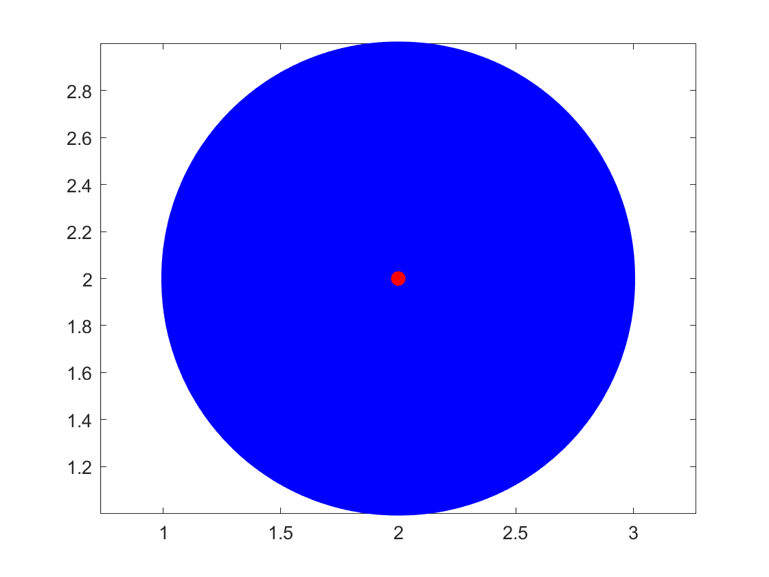
(a) the 2D plot of rotation

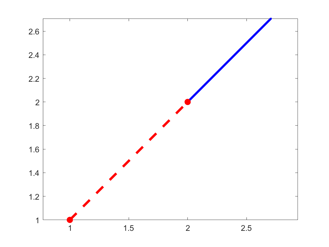
(b) the 2D plot of translation

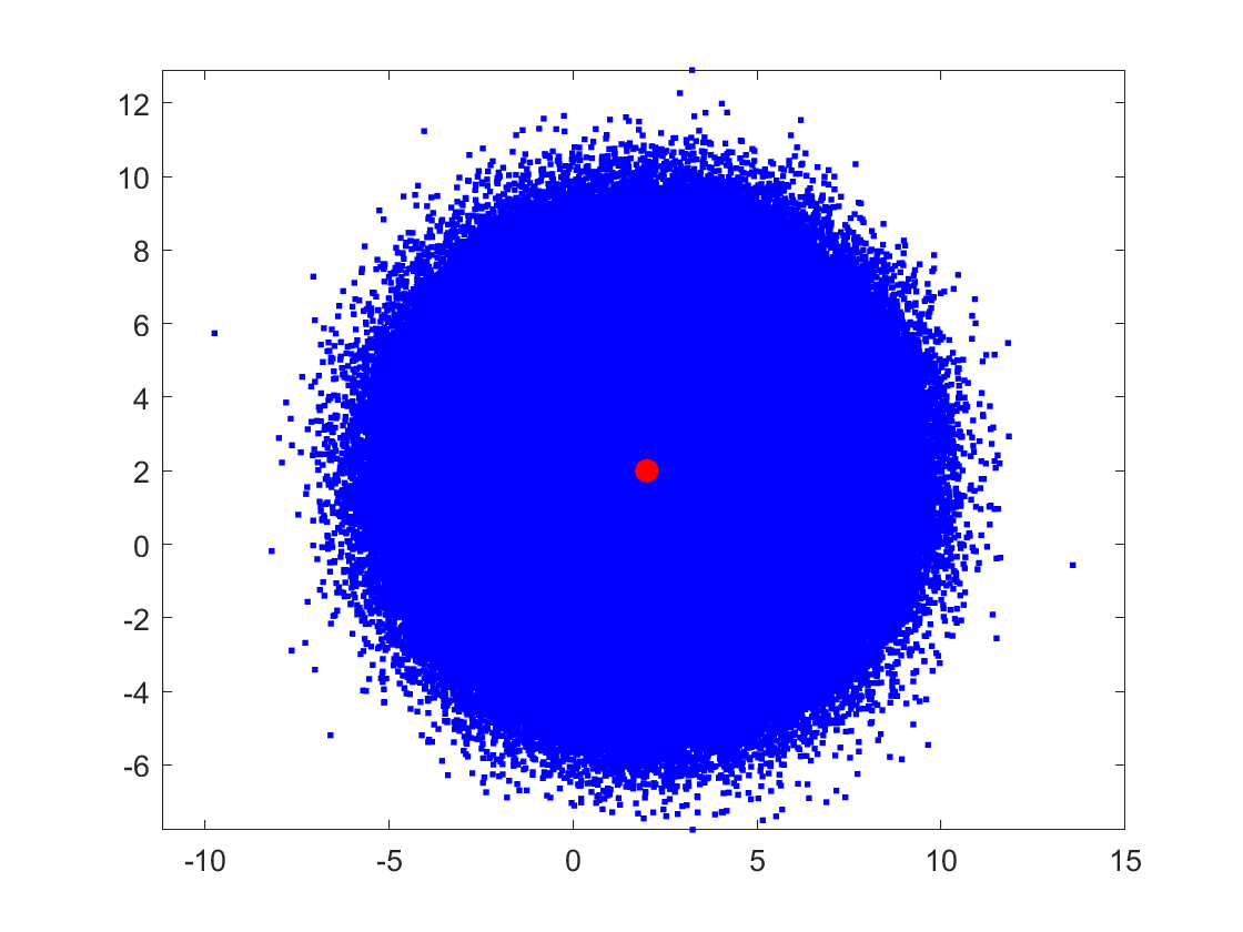
(c) the 2D plot of expansion

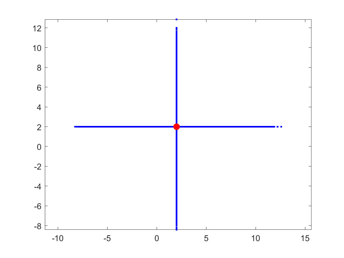
(d) the 2D plot of axesion

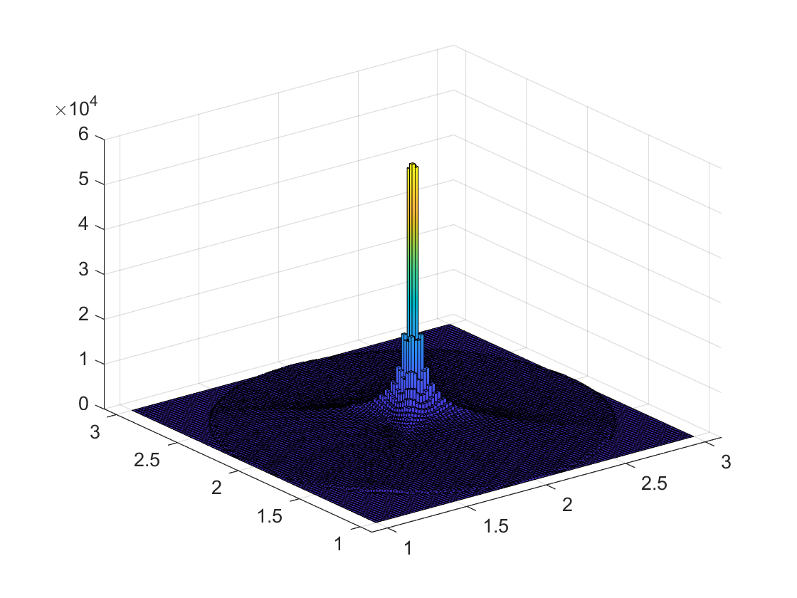
(e) the 3D histogram of rotation

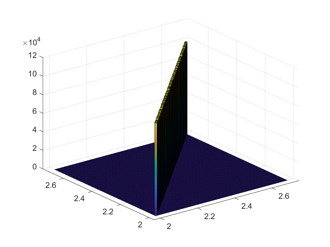
(f) the 3D histogram of translation

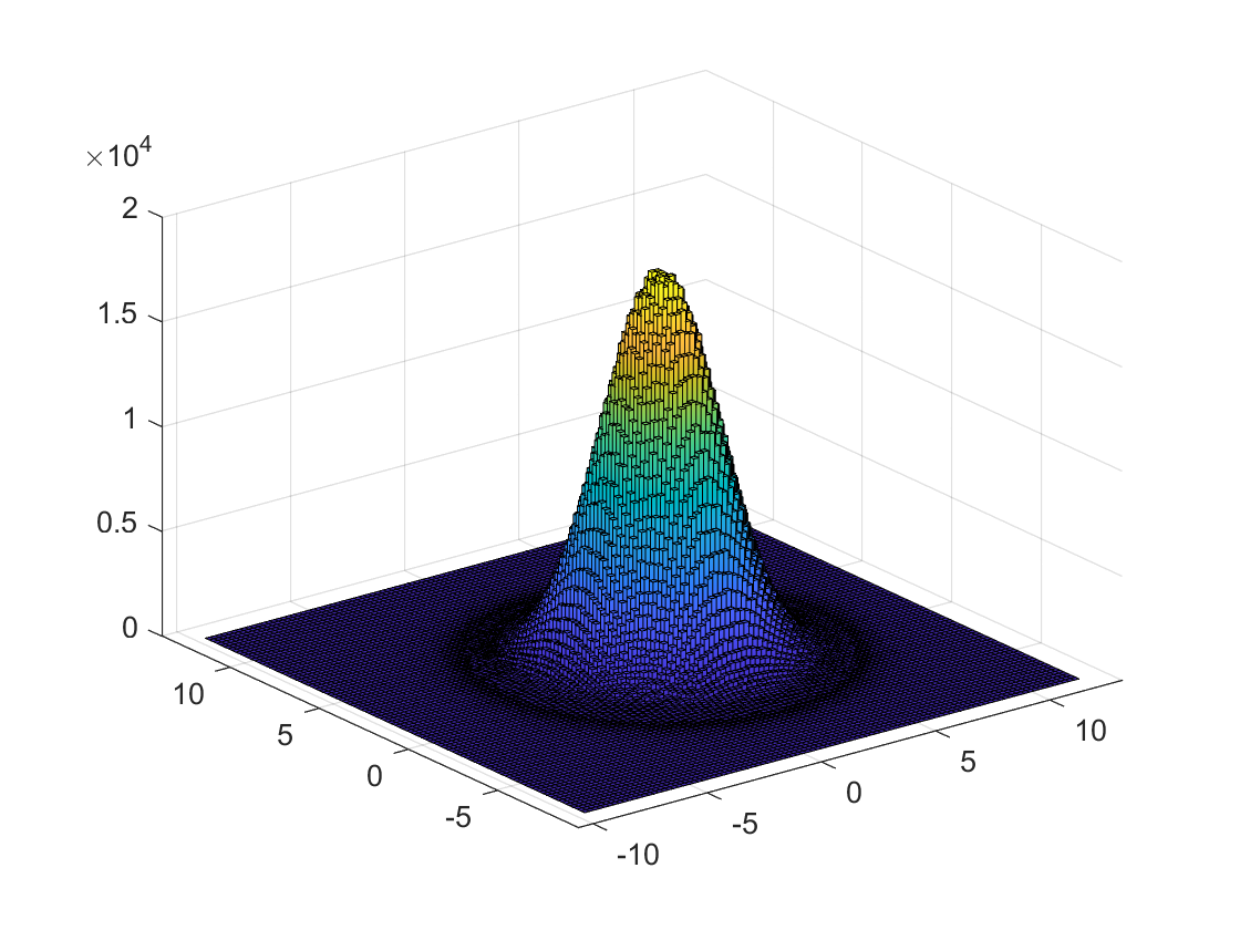
(g) the 3D histogram of expansion

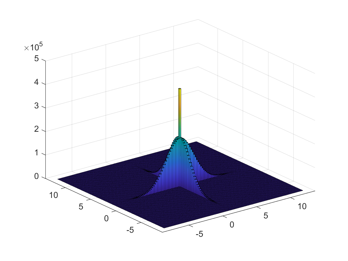
(h) the 3D histogram of axesion

Figure 1: Illustration of the 2D plot and 3D histogram of state transformations

With the state transformation operators, sampling technique and update strategy, the basic state transition algorithm can be described by the following pseudocode

1:repeat

2:  if $\alpha<\alpha_{\min}$ then

3:   $\alpha\leftarrow\alpha_{\max}$

4:  end if

5:  Best $\leftarrow$ expansion(funfcn,Best,SE,$\beta$,$\gamma$)

6:  Best $\leftarrow$ rotation(funfcn,Best,SE,$\alpha$,$\beta$)

7:  Best $\leftarrow$ axesion(funfcn,Best,SE,$\beta$,$\delta$)

8:  $\alpha\leftarrow\frac{\alpha}{\textit{fc}}$

9:until the termination criterion is satisfied

where, SE is the sample size, and the termination criterion is usually the maximum number of iterations, or the the maximum number of function evaluations. The update strategy $f(\bm{Best}_{k+1})\leq f(\bm{Best}_{k})$ is used to update incumbent best solution. For details, please refer to [1].

II-B The principle behind the STA

The goal of STA is to find a global or near-global optimal solution to a general continuous optimization problem as soon as possible. As a constructivism-based intelligent optimization method, STA possesses the following five core structural elements:

• Globality: the capability to explore the entire search space;

• Optimality: the guarantee of obtaining an optimal solution;

• Rapidity: reducing computational complexity as much as possible;

• Convergence: guaranteeing the convergence of the generated sequence;

• Controllability: flexibly managing the search space.

The globality mainly lies in the expansion transformation operator. Since $R_{e}$ is a random diagonal matrix with its entries obeying the Gaussian distribution, using the expansion transformation with a nonzero vector $\bm{s}_{k}$ and sufficiently large expansion factor $\gamma$, the entries in $\bm{s}_{k+1}$ can be expanded to the range of $(-\infty,+\infty)$, from the perspective of probability theory.

The optimality mainly lies in the rotation transformation operator. It is proved that $\|\bm{s}_{k+1}-\bm{s}_{k}\|\leq\alpha$ by using the rotation transformation. That is to say, with a sufficiently large sample size SE and sufficiently small rotation factor $\alpha_{\min}$, if no better candidate $\bm{s}_{k+1}$ is found, the incumbent $\bm{s}_{k}$ can be regarded as an optimal solution in the mathematical sense, achieved with a prescribed level of precision.

The rapidity lies in several aspects: i) the sampling technique; based on the incumbent, all candidates generated by each state transformation operator can form a regular neighborhood, and then representative candidates can be obtained by sampling, avoiding complete enumeration. ii) the alternate strategy; the alternative use of various transformation operators accelerates the escape from the region around a local optimum. iii) efficient implementation; for example, the time complexity of the rotation transformation implementation has been reduced from $O(n^{2})$ to $O(n)$ [19].

The convergence mainly lies in the update strategy: $f(\bm{Best}_{k+1})\leq f(\bm{Best}_{k})$. Since the sequence $\{f({\bm{Best}}_{k})\}$ is monotonically decreasing and $f(\bm{Best})$ is bounded below, the sequence $\{f({\bm{Best}}_{k})\}$ converges.

The controllability mainly lies the transformation factors $\alpha,\beta,\gamma$ and $\delta$. These transformation factors can regulate the search space to a desired region with a specific size. For example, the rotation transformation enables searching within a hypersphere of maximal radius $\alpha$.

Theorem 1.

If the sample size SE is sufficiently large and the rotation factor $\alpha$ is sufficiently small at later stage, the sequence $\{f({\bm{Best}}_{k})\}$ generated by the STA can at least converge to a local minimum, i.e.,

$$\lim_{k\rightarrow\infty}f(\bm{Best}_{k})=f(\bm{x}^{*})$$ (7)

where $\bm{x}^{*}$ is a local minimum.

Proof.

Firstly, since the update strategy $f(\bm{Best}_{k+1})\leq f(\bm{Best}_{k})$ is used in the STA, the $\{f({\bm{Best}}_{k})\}$ is monotonically decreasing, and $f(\bm{Best_{k}})$ is bounded below, according to the monotone convergence theorem, the sequence $\{f({\bm{Best}}_{k})\}$ converges to $f(\bm{x}^{*})$.

Secondly, since the sample size SE is sufficiently large and the rotation factor $\alpha$ is sufficiently small, it is not difficult to derive that $f(\bm{Best}_{k})\leq f(\bm{s}_{k+1}),\forall\bm{s}_{k+1}\in\mathcal{S}$, where $\mathcal{S}=\{\bm{s}|\|\bm{s}-\bm{Best}_{k}\|\leq\alpha_{\min}\}$ is the neighborhood of $\bm{Best}_{k}$, that it to say, $f(\bm{Best}_{k})$ can be considered as a local minimum with solution accuracy $\alpha_{\min}$.

To sum up, the sequence $\{f({\bm{Best}}_{k})\}$ generated by the STA can at least converge to a local minimum with certain solution accuracy. ∎

II-C Analysis of the termination conditions used in intelligent optimization

In intelligent optimization, the majority of studies focus on generating candidate solutions and updating incumbent solutions, to achieve the balance between global exploration and local exploitation. The termination conditions are often ignored, and the maximum number of iterations is usually set as the termination condition. However, the termination conditions are significant when solving real-world optimization problems. If they are set too small, the algorithm may fail to find the optimal solution; on the contrary, if set too large, the algorithm may result in a waste of computing resources. As a result, extensive trial and error is required, which is not feasible in a time-constrained environment. In academic community, the indicators to termination criteria can be summarized into the following three categories [14, 15]:

1. Resource indicators

   • the maximum number of generations or iterations;

   • the maximum number of function evaluations;

   • the maximum CPU time.

2. Progress indicators

   • accuracy, i.e., the distance to the optimum is less than a given tolerance;

   • hitting a bound, i.e., the best found objective function value hits a given bound;

   • $K$-iterations, i.e., there is no obvious improvement after $K$ consecutive generations or iterations.

3. Characteristic indicators

   • convergence;

   • diversity;

   • clustering;

   • statistic.

Even though various termination criteria have already been used in intelligent optimization, how to determine a suitable termination criterion for the majority of intelligent optimization algorithms still remains an open problem since the best solution found may not be strictly optimal in mathematics when resources are exhausted, progress has stagnated or several characteristics are present. Fortunately, as mentioned before, the STA has the potential to design a termination condition that can guarantee a strictly optimal solution due to its intrinsic characteristics.

III Proposed efficient STA

Considering that the standard STA shows slow convergence at a later stage for flat landscape functions, novel state transformations and parameter adaptation strategy are proposed to accelerate the convergence in this section.

III-A Novel translation transformation based on predictive modeling

In STA, the translation transformation is utilized a heuristic search to generate more potential solutions, and it can search along a line from previous best solution to current best solution. This is intuitive and straightforward since current best solution is better than previous best solution. From the perspective of regression analysis, the translation transformation in standard STA is a first-order predictive model with normalized scale, but only the last best solution is utilized. To make sufficient utilization of historical best solutions, in this part, new translation transformations based on first and second order predictive models are proposed.

Firstly, let us recall the widely used autoregressive integrated moving average ARIMA($p,d,q$) model [20, 21]:

$$\bm{x}_{t}=\bm{c}+\sum_{i=1}^{p}\phi_{i}\bm{x}_{t-i}+\bm{\epsilon}_{t}+\sum_{i=1}^{q}\theta_{i}\bm{\epsilon}_{t-i},$$ (8)

where $\bm{x}_{t}$ is the actual value, $\bm{\epsilon}_{t}$ is the Gaussian white noise, $p$ and $q$ are called autoregressive order and moving average order, respectively. $d$ is the degree of differencing.

To make sure that the series can converge, new translation transformations based on the first and second order predictive models are proposed as follows

$$\bm{s}_{k+1} =\bm{s}_{k}+\beta\hat{R}_{t}(\bm{s}_{k}-\bm{s}_{k-1}),$$ (9a)

$$\bm{s}_{k+1} =\bm{s}_{k}+\beta\hat{R}_{t}(\bm{s}_{k-1}-\bm{s}_{k-2}),$$ (9b)

where $\bm{s}_{k}$ represents the current state, $\bm{s}_{k-1}$ and $\bm{s}_{k-2}$ are historical states. $\hat{R}_{t}$ $\in\mathbb{R}$ is a uniformly distributed random variable defined on the interval [-1,1]. Furthermore, to reflect the influence of the degree of differencing $d$, $\bm{s}_{k-1}$ and $\bm{s}_{k-2}$ are chosen randomly from the historical best archive.

The differences between the first and the second order predictive models are illustrated in Fig. 2. With the same previous best solutions $A,B,C$, the current best solution $D$, the next candidate solutions $A^{\prime},B^{\prime},C^{\prime}$ are different using different predictive models. In the first order predictive model, $A$, $D$, and $A^{\prime}$ are in the same line, the same to $B$, $D$, and $B^{\prime}$, $C$, $D$, and $C^{\prime}$. In the second order predictive model, the line $AB$ is parallel to line $DA^{\prime}$, the same to line $BC$ and line $DB^{\prime}$, line $AC$ and line $DC^{\prime}$. Although the newly generated solutions are different, the convergence rate is manipulated the same term $\beta\hat{R}_{t}$, as shown in Eq. (9).

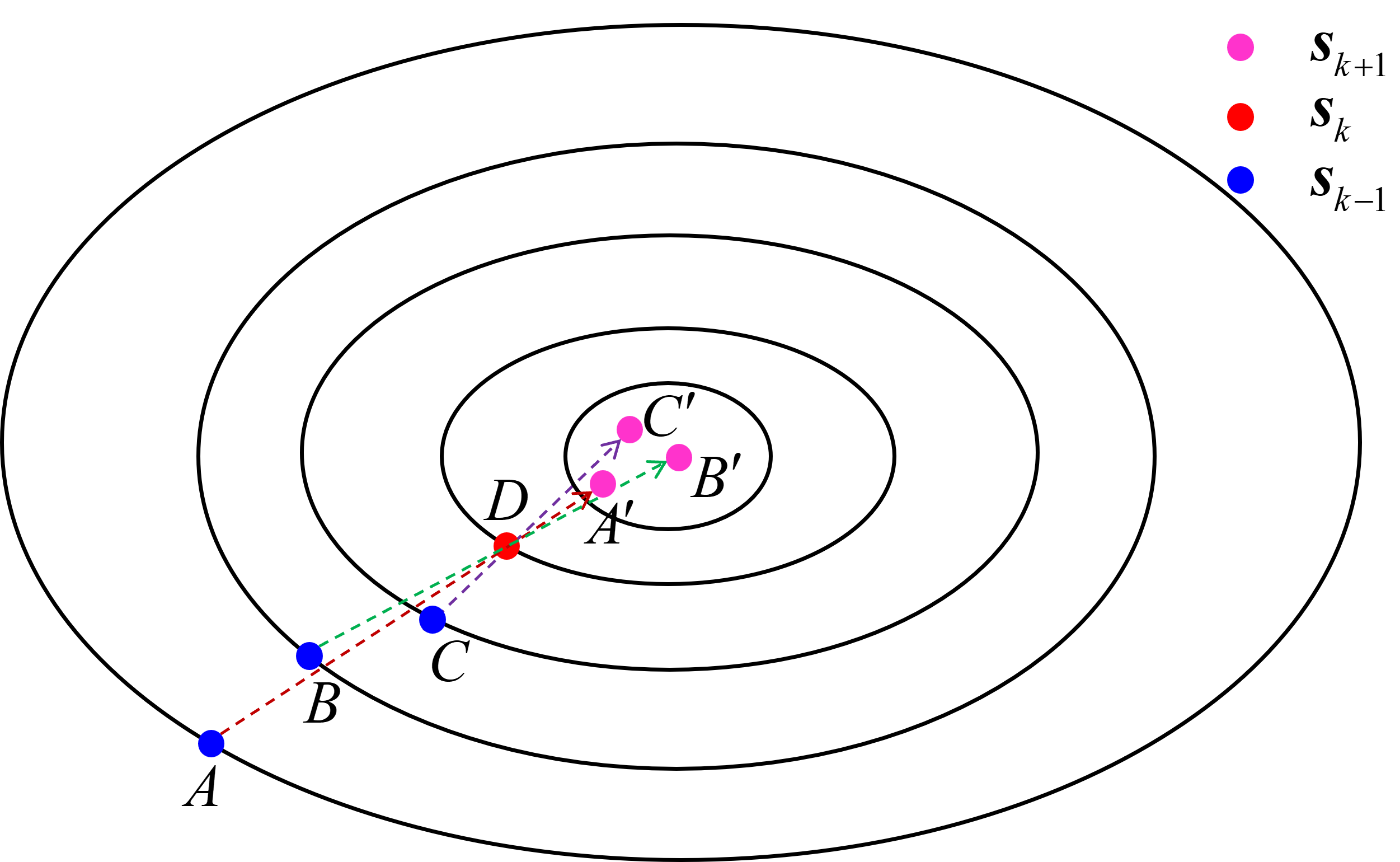
(a)

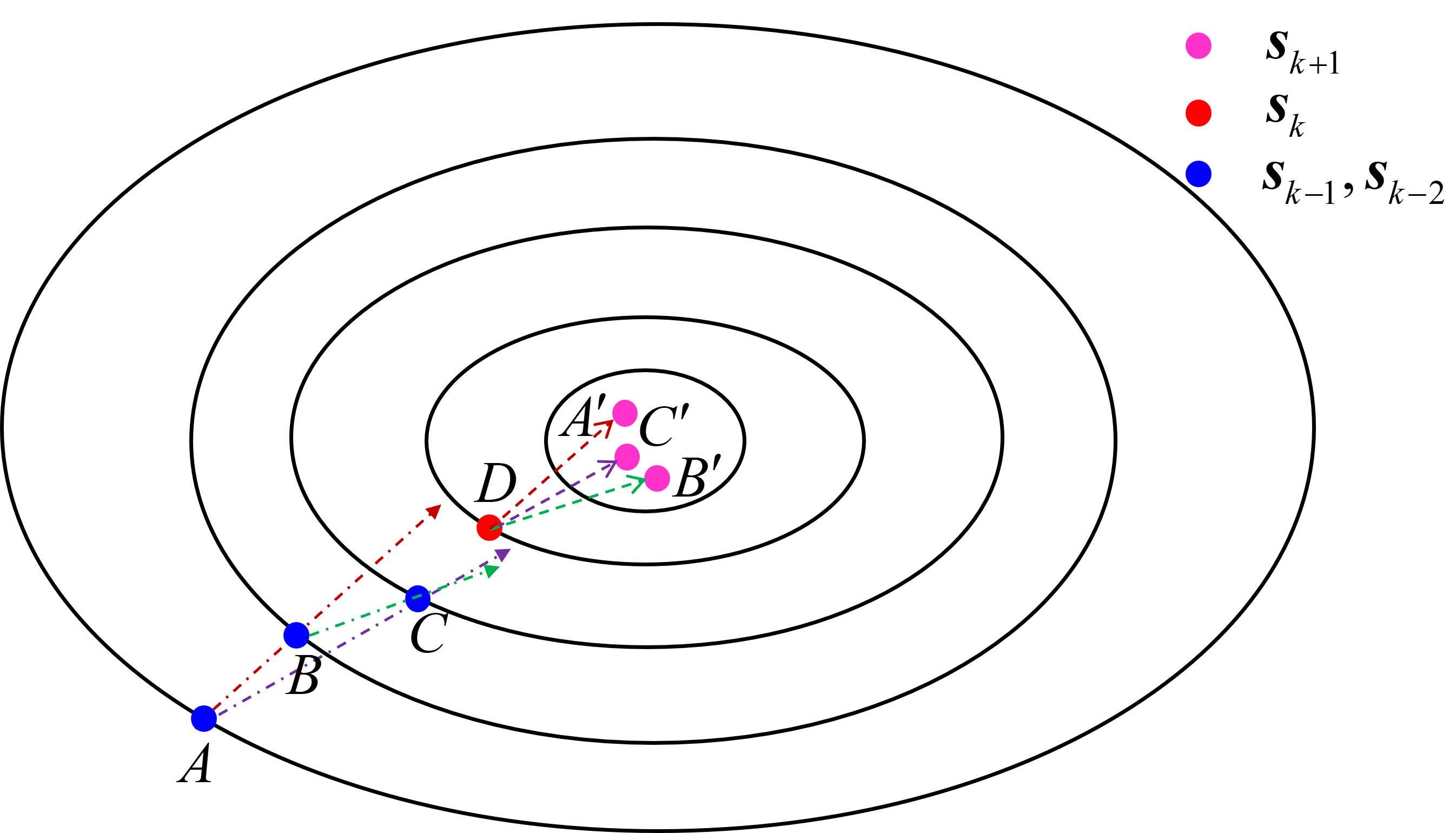
(b)

Figure 2: Illustration and comparison of the two new translation transformations

III-B New expansion and axesion transformation for supplementation

In standard STA, the expansion transformation is designed for global search, while the axesion transformation aims for heuristic search. Although these two transformation operators perform well in most scenarios, their effectiveness diminishes in an extreme case. As shown in Fig. 3, the global point $B$ (where $x=2$) is far away from the local point point $A$ (where $x=0.2$). If the incumbent best solution $s_{k}$ is around the local point $A$ and the state transformation factor is set at 1, it is extremely difficult to jump out of the neighborhood since the probability $P(s_{k+1}\geq 0.8)\approx 0.13\%$ .

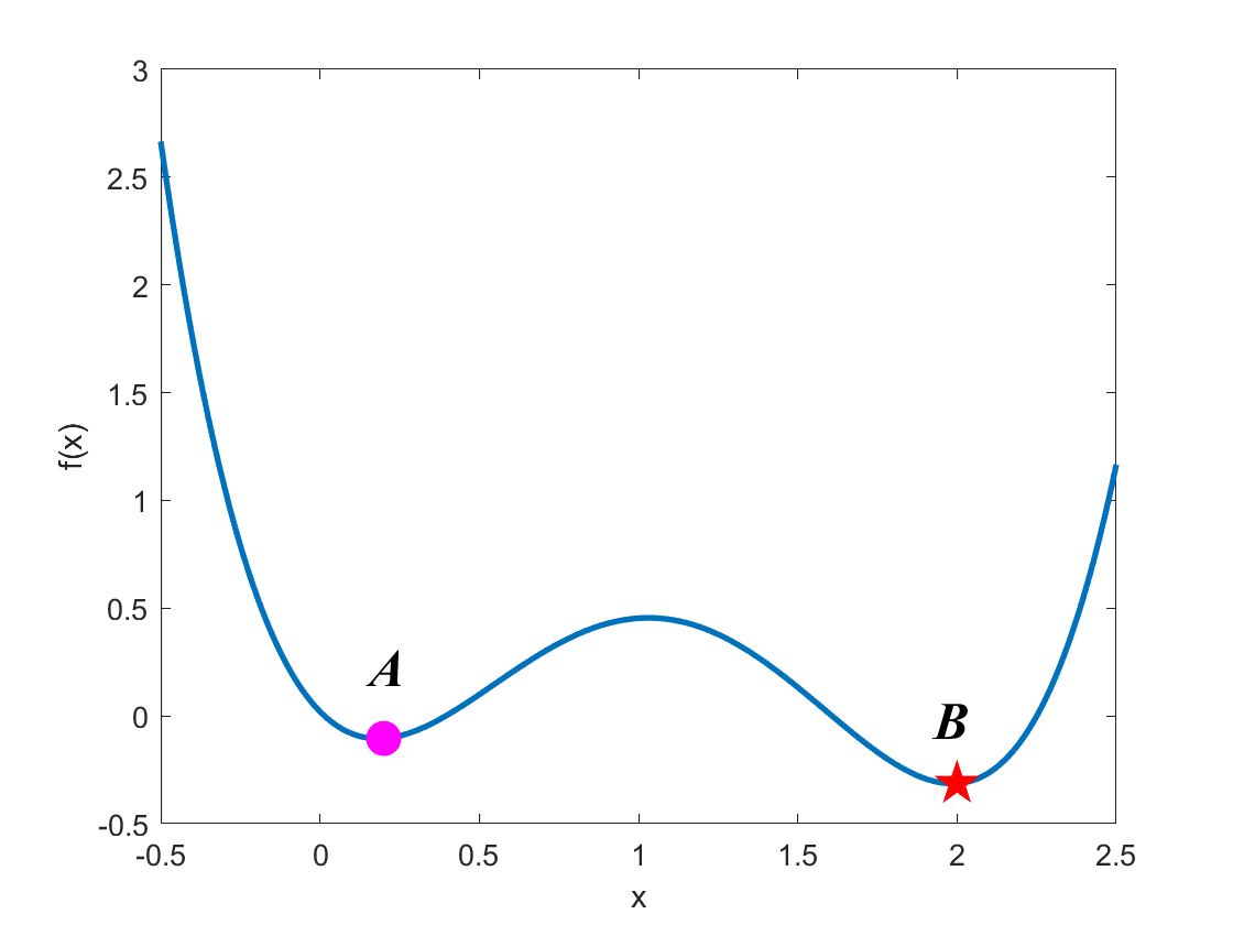
Figure 3: The illustration of an extreme case

To resolve the above-mentioned issue, new expansion and axesion transformation are designed as follows.

$$\mathrm{expansion}:\bm{s}_{k+1} =\bm{s}_{k}+\gamma R_{e}\bm{u}_{k},$$ (10)

$$\mathrm{axesion}:\bm{s}_{k+1} =\bm{s}_{k}+\gamma R_{a}\bm{u}_{k}.$$

where $\bm{u}_{k}=[1,\cdots,1]^{T}$ is the all-ones vector.

Remark 1.

For the extreme case, by using the new axesion transformation, the the probability to jump out of the local point $A$ is $P(s_{k+1}\geq 1)\approx 21\%$. Given that the original expansion and axesion transformation perform well in most cases, these new transformations are therefore combined with the original ones.

III-C Proposed parameter control strategy

Parameter setting is one of the key issues in intelligent optimization algorithms since their performance depends greatly on the parameter values. The parameter setting can be classified into parameter tuning and parameter control. In parameter tuning, optimal parameter values are carefully selected and kept constant throughout the execution of the optimization process. In contrast, parameter control dynamically adjusts parameter values during the optimization process to enhance performance and adaptability. Given that finding optimal parameter values is challenging and time-consuming, and there exists no fixed set of parameters adaptable to all optimization problems, parameter control becomes essential, especially for complex optimization problems.

Parameter setting is also important in STA, as it has been observed that the state transformation factors have a significant impact on the performance of STA. In standard STA [5], the translation factor $\beta$, the expansion factor $\gamma$, and the axesion factor $\delta$ are held constant, while the rotation factor $\alpha$ decreases exponentially from 1 to $10^{-4}$ with a base of 2 in a periodic manner. In dynamic STA (DynSTA) [19], all state transformation factors decrease exponentially from 1 to $10^{-4}$ with a base of 2 in a periodic fashion to enhance local exploitation in the later stages. In parameter-optimal STA (POSTA) [1], an optimal parameter selection strategy is proposed to accelerate convergence. Specifically, the optimal state transformation factors are selected from a set $\{1,10^{-1},10^{-2},\dots,10^{-8}\}$, and they are held constant for a predefined period to ensure full utilization.

III-C1 An intuitive parameter adaptation strategy

Firstly, we focus on investigating two key state transformation factors: the rotation factor $\alpha$ and the expansion factor $\gamma$, which account for local search and global search, respectively. The central idea is to adjust these parameters according to changes in the incumbent solution. As is well known, larger parameter values facilitate global exploration, while smaller values benefit local exploitation. Moreover, it is widely accepted that global search should be emphasized in the early stages to explore unknown regions, while local search should be strengthened in the later stages to exploit discovered regions and refine the solution. Based on our previous research, we have found that setting the state transformation factors to 1 offers a balanced and moderate approach. If the value is set too high, it generates redundant and invalid candidate solutions, resulting in inefficiency. On the other hand, if the value is set too low during the early stages, progress in improving the solution slows down.

Based on the above analysis, an intuitive parameter adaptation strategy in proposed as shown in Fig. 4, where the change in consecutive two incumbent solution is defined as follows:

$$\triangle x=\max(\left|\bm{Best}_{k}-\bm{Best}_{k-1}\right|)$$ (11)

here, $\bm{Best}_{k}$ and $\bm{Best}_{k-1}$ are current best solution and previous best solution, respectively. It utilizes the maximum variation in two incumbent solutions as the indicator to adjust the state transformation factors $\alpha$ and $\gamma$.

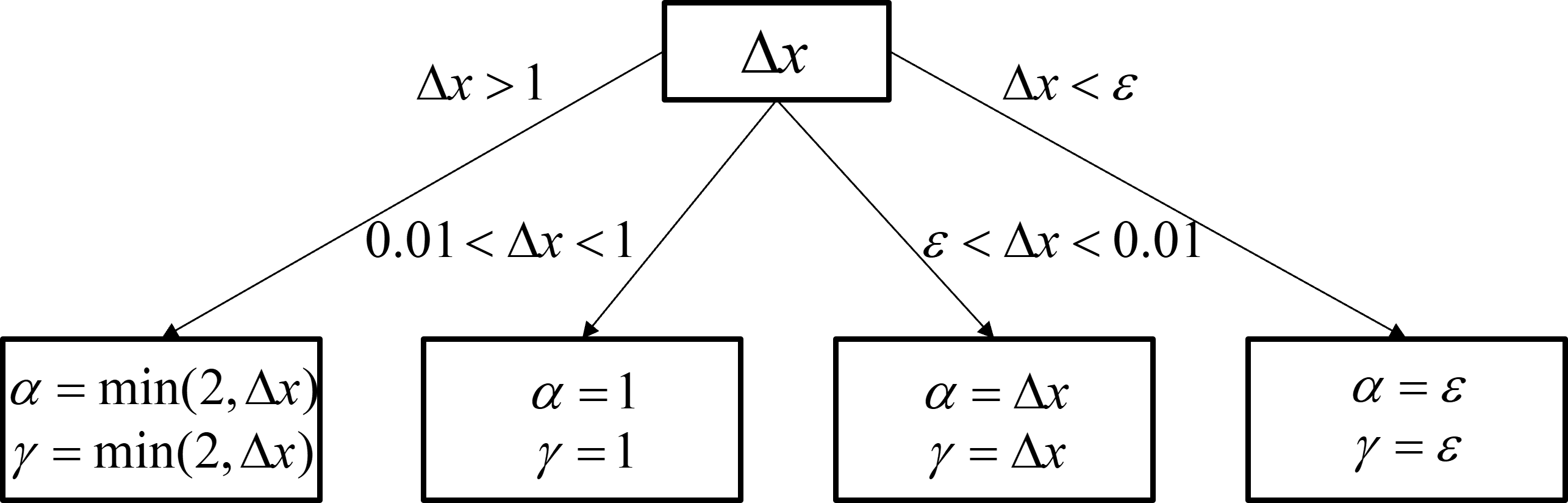
Figure 4: An intuitive parameter adaptation strategy

III-C2 Parameter optimal selection strategy

On the other hand, as indicated in POSTA [1], the impact of parameter on STA is predictable, as its parameter is analogous to the learning rate, also known as the step size in gradient-based optimization algorithms, as shown below

$$\left.\begin{array}[]{l}R_{r}\frac{\bm{u}_{k}}{\|\bm{u}_{k}\|_{2}}\\ \hat{R}_{t}(\bm{s}_{k}-\bm{s}_{k-1})\\ \cdots\end{array}\right\}\Rightarrow\bm{d}_{k},\left.\begin{array}[]{l}\alpha\\ \beta\\ \cdots\end{array}\right\}\Rightarrow a_{k},\bm{s}_{k+1}=\bm{s}_{k}+a_{k}\bm{d}_{k},$$

where $\bm{d}_{k}$ is analogous to the search direction in trust region methods.

Assuming that the incumbent solution is not optimal, if the parameter is sufficiently small, there must exist better candidate solutions obtained through the corresponding state transformation operator. However, if the parameter is too large or inappropriate, inefficient search will occur.

With this in mind, the parameter selection problem is analogous to the line search in traditional mathematical programming methods. For simplicity, an inexact but suboptimal line search strategy is introduced as follows

$$a^{*}=\operatorname*{arg\,min}_{a_{k}\in\Omega}f(\bm{s}_{k}+a_{k}\bm{d}_{k})$$ (12)

where, $\Omega=\{2,1,10^{-1},10^{-2},\dots,10^{-8}\}$.

III-D Proposed efficient STA with guaranteed optimality

With the above state transformation operators and parameter control strategies, the procedures of the proposed efficient STA with guaranteed optimality is given as follows

1:repeat

2:  prevfBest $\leftarrow$ fBest

3:  [Best,fBest,Archive] $\leftarrow$ expansion(*,Best,Archive,$\gamma$)

4:  [Best,fBest,Archive] $\leftarrow$ rotation(*,Best,Archive,$\alpha$)

5:  [Best,fBest,Archive] $\leftarrow$ axesion(*,Best,Archive,$\delta$)

6:  [Best,fBest,Archive] $\leftarrow$ translation(*,Best,Archive,$\beta$)

7:  [$\alpha,\beta,\gamma,\delta$] $\leftarrow$ UpdateParameter()

8:until $\mathrm{fBest}==\mathrm{prevfBest}\;\&\;\alpha\leq\epsilon$

where, the Archive is to store historical best solutions and $\epsilon$ is the solution accuracy.

Remark 2.

The designed termination condition indicates that if the rotation factor $\alpha$ decreases below a predefined threshold $\epsilon$ without any further progress ($\mathrm{fBest}==\mathrm{prevfBest}$), the STA will terminate automatically. By the way, to distinguish between different parameter control strategies, the proposed STA, which incorporates an intuitive parameter adaptation strategy that is simple yet efficient, is abbreviated as ESTA. In the meanwhile, the extended version that employs the optimal parameter selection strategy is called EXSTA.

IV Experimental results and analysis

IV-A Experimental setup

In this part, extensive experiments are conducted to evaluate the performance of the proposed effective STA. To avoid redundant comparisons among functions with similar characteristics, a set of representative benchmark functions was selected, as presented in Table I. Although the number of functions is not too large, they cover a diverse range of types, including Type I: unimodal $(f_{1},f_{6},f_{9})$ and multimodal $(f_{2},f_{3},f_{4},f_{5},f_{7},f_{8},f_{10})$; Type II: all-zero optimal solution $(f_{1},f_{3},f_{4},f_{5})$ and non-zero optimal solution $(f_{2},f_{6},f_{7},f_{8},f_{9},f_{10})$; Type III: identical optimal solution $(f_{1},f_{2},f_{3},f_{4},f_{5},f_{7},f_{10})$ and nonidentical optimal solution $(f_{6},f_{8},f_{9})$; Type IV: separable $(f_{1},f_{3},f_{6},f_{7},f_{10})$, and nonseparable $(f_{2},f_{4},f_{5},f_{8},f_{9})$; Type V: flatten $(f_{2},f_{8},f_{9})$, and unflatten $(f_{1},f_{3},f_{4},f_{5},f_{6},f_{7},f_{10})$.

For a comprehensive evaluation, firstly, we compared the proposed effective STA with STA variants, including the standard STA [5], DynSTA [19] and POSTA [1]. Then, the proposed effective STA is compared with several other representative intelligent optimization algorithms, including some well-established methods like GL25 [22], CLPSO [23], CMAES [24], and SaDE [25], as well as some recently popular methods like GWO [26], WOA [27], HHO [28] and SMA [29]. When compared to other optimization algorithms, the experiment is divided into two groups based on the termination conditions: Maximum Stall Iterations (MaxStalls) and Maximum Function Evaluations (MaxFEs). Each function is tested with 20, 30 and 50 dimensions, and all algorithms are independently run 30 times in MATLAB (version R2022b) on a PC with Intel(R) Core(TM) i7-1260P CPU @2.10 GHz.

For the parameter settings, the parameters in other optimization algorithms are set to their default values. In STA and its variants, the sample size SE is set to 30. For the designed termination conditions, when $\mathrm{prefBest}-\mathrm{fBest}\leq\mathrm{eps}$ (a constant in MATLAB), it is considered that $\mathrm{fBest}==\mathrm{prevfBest}$, and the accuracy of solution $\epsilon$ is set to $10^{-8}$. When applying the optimal parameter selection strategy, the hyperparameters are set to be the same as those in POSTA.

TABLE I: The used benchmark functions

Name	Function	Range	$x^{*}$	$f(x^{*})$
Sphere	$f_{1}(\bm{x})=\displaystyle\sum_{i=1}^{n}x_{i}^{2}$	[-100, 100]	[0,$\cdots$,0]	0
Rosenbrock	$f_{2}(\bm{x})=\displaystyle\sum_{i=1}^{n}(100(x_{i+1}-x_{i}^{2})^{2}+(x_{i}-1)^{2})$	[-30, 30]	[1,$\cdots$,1]	0
Rastrigin	$f_{3}(\bm{x})=\displaystyle\sum_{i=1}^{n}(x_{i}^{2}-10\cos(2\pi x_{i})+10)$	[-5.12, 5.12]	[0,$\cdots$,0]	0
Griewank	$f_{4}(\bm{x})=\frac{1}{4000}\displaystyle\sum_{i=1}^{n}x_{i}^{2}-\prod_{i=1}^{n}\cos(\frac{x_{i}}{\sqrt{i}})+1$	[-600, 600]	[0,$\cdots$,0]	0
Ackley	$f_{5}(\bm{x})=20+e-20\exp\Big{(}-0.2\scriptstyle{\sqrt{\frac{1}{n}\displaystyle\sum_{i=1}^{n}x_{i}^{2}}}\Big{)}-\exp\Big{(}\frac{1}{n}\displaystyle\sum_{i=1}^{n}\cos(2\pi x_{i})\Big{)}$	[-32, 32]	[0,$\cdots$,0]	0
Quadconvex	$f_{6}(\bm{x})=\displaystyle\sum_{i=1}^{n}(x_{i}-i)^{2}$	$[-10n,10n]$	[1,$\cdots$,$n$]	0
Schwefel	$f_{7}(\bm{x})=\displaystyle\sum_{i=1}^{n}-x_{i}\sin(\sqrt{|x_{i}|})+418.9828872724338n$	[-500, 500]	[420.9687,$\cdots$,420.9687]	0
Michalewicz	$f_{8}(\bm{x})=-\displaystyle\sum_{i=1}^{n}\sin(x_{i})\sin(\frac{ix_{i}^{2}}{\pi})^{20}$	[0, $\pi$]	unknown	unknown
Trid	$f_{9}(\bm{x})=\displaystyle\sum_{i=1}^{n}(x_{i}-1)^{2}-\displaystyle\sum_{i=2}^{n}x_{i}x_{i-1}+\frac{n(n+4)(n-1)}{6}$	$[-n^{2},n^{2}]$	$x_{i}^{*}=i(n+1-i)$	0
Giunta	$\begin{array}[]{l}f_{10}(\bm{x})=\displaystyle\sum_{i=1}^{n}[\sin(ax_{i}-1)+\sin^{2}(ax_{i}-1)+b\sin(4(ax_{i}-1))]\\ +0.2677647897315472n,a=\frac{16}{15},b=\frac{1}{50}\end{array}$	$[-1,1]$	[0.4673,$\cdots$,0.4673]	0

IV-B Comparison among different predictive models

As mentioned in Section III, there will be three types of predictive models: the first order model, the second order model, and their hybrid model. In this part, a comparison is conducted to examine the differences among these models.Different predictive models based ESTA with designed termination conditions are compared, and the statistical results are shown in Table II. The mean (denoted as m) and standard deviation (denoted as sd) of the objective function values (abbreviated as ObjVal) are used to evaluate the search capability and stability of the algorithms. In the meanwhile, the mean of gradient norm (abbreviated as GradNorm) is used to assess optimality.

From the statistical results in Table II, it is found that all predictive models based ESTA with designed termination conditions can be considered to have achieved optimality, as the magnitude of the gradient norm is $10^{-4}$ or less (most engineering applications choose this precision). Almost all predictive models based ESTA are able to find the global optimal solution with a certain level of precision, except for the Griewank function in 20 dimensions, and the Michalewicz function since its global optimal solution is unknown. On the other hand, by combining the Wilcoxon rank-sum test results in the Table III, no significant difference is observed among these models.

TABLE II: Comparison of different predictive models based ESTA with designed termination conditions

Fcn	Dim	1st model		2nd model		Hybrid model
		ObjVal (m $\pm$ sd)	GradNorm (m)	ObjVal (m $\pm$ sd)	GradNorm (m)	ObjVal (m $\pm$ sd)	GradNorm (m)
	20	6.49e-16 $\pm$ 3.78e-16	5.11e-08	5.36e-16 $\pm$ 2.42e-16	4.75e-08	6.60e-16 $\pm$ 3.85e-16	5.07e-08
$f_{1}$	30	1.13e-15 $\pm$ 5.55e-16	6.71e-08	1.07e-15 $\pm$ 4.74e-16	6.80e-08	1.26e-15 $\pm$ 5.73e-16	7.05e-08
	50	2.51e-15 $\pm$ 8.98e-16	1.00e-07	2.90e-15 $\pm$ 1.07e-15	1.06e-07	2.55e-15 $\pm$ 8.53e-16	1.04e-07
	20	1.67e-14 $\pm$ 9.20e-15	4.44e-06	1.60e-14 $\pm$ 9.85e-15	4.08e-06	1.71e-14 $\pm$ 1.37e-14	3.93e-06
$f_{2}$	30	4.22e-14 $\pm$ 3.14e-14	6.36e-06	3.93e-14 $\pm$ 3.18e-14	5.87e-06	3.31e-14 $\pm$ 1.53e-14	5.76e-06
	50	9.22e-14 $\pm$ 6.28e-14	9.82e-06	9.09e-14 $\pm$ 4.84e-14	9.40e-06	7.29e-14 $\pm$ 4.03e-14	8.88e-06
	20	1.36e-13 $\pm$ 7.50e-14	1.23e-05	1.91e-13 $\pm$ 8.78e-14	1.47e-05	1.58e-13 $\pm$ 8.02e-14	1.32e-05
$f_{3}$	30	5.76e-13 $\pm$ 2.51e-13	2.32e-05	5.74e-13 $\pm$ 2.17e-13	2.37e-05	5.87e-13 $\pm$ 2.68e-13	2.32e-05
	50	1.62e-12 $\pm$ 4.62e-13	3.70e-05	1.77e-12 $\pm$ 6.45e-13	3.99e-05	1.70e-12 $\pm$ 6.32e-13	3.78e-05
	20	1.23e-02 $\pm$ 1.55e-02	1.73e-08	1.67e-02 $\pm$ 1.92e-02	1.65e-08	2.19e-02 $\pm$ 2.27e-02	1.75e-08
$f_{4}$	30	1.69e-15 $\pm$ 8.15e-16	1.89e-08	2.13e-15 $\pm$ 1.35e-15	2.07e-08	1.57e-15 $\pm$ 1.70e-15	1.80e-08
	50	4.44e-15 $\pm$ 4.28e-15	2.30e-08	3.82e-15 $\pm$ 2.08e-15	2.43e-08	4.19e-15 $\pm$ 3.01e-15	2.27e-08
	20	3.10e-13 $\pm$ 1.60e-13	1.15e-06	3.82e-13 $\pm$ 2.99e-13	4.08e-06	4.09e-13 $\pm$ 3.27e-13	2.15e-06
$f_{5}$	30	4.14e-12 $\pm$ 4.18e-12	3.27e-06	3.48e-12 $\pm$ 4.15e-12	3.27e-06	9.03e-13 $\pm$ 6.73e-13	6.18e-06
	50	3.94e-12 $\pm$ 3.41e-12	3.49e-06	2.88e-12 $\pm$ 2.17e-12	9.49e-06	6.95e-12 $\pm$ 7.68e-12	7.71e-06
	20	1.72e-15 $\pm$ 7.59e-16	8.11e-08	1.88e-15 $\pm$ 7.46e-16	8.50e-08	1.76e-15 $\pm$ 8.28e-16	8.62e-08
$f_{6}$	30	3.33e-15 $\pm$ 1.41e-15	1.13e-07	3.52e-15 $\pm$ 1.24e-15	1.19e-07	3.57e-15 $\pm$ 1.74e-15	1.23e-07
	50	9.87e-15 $\pm$ 2.43e-15	2.03e-07	1.05e-14 $\pm$ 2.21e-15	2.13e-07	9.18e-15 $\pm$ 3.16e-15	1.96e-07
	20	1.72e-11 $\pm$ 7.54e-12	2.97e-06	2.26e-11 $\pm$ 1.19e-11	3.30e-06	2.22e-11 $\pm$ 1.11e-11	3.35e-06
$f_{7}$	30	5.79e-11 $\pm$ 2.28e-11	5.46e-06	5.56e-11 $\pm$ 2.16e-11	5.32e-06	5.60e-11 $\pm$ 2.10e-11	5.41e-06
	50	1.67e-10 $\pm$ 5.08e-11	9.27e-06	1.78e-10 $\pm$ 7.22e-11	9.44e-06	1.79e-10 $\pm$ 6.81e-11	9.20e-06
	20	-1.96e+01 $\pm$ 1.34e-02	1.95e-05	-1.96e+01 $\pm$ 1.23e-02	2.15e-05	-1.96e+01 $\pm$ 1.29e-02	2.15e-05
$f_{8}$	30	-2.96e+01 $\pm$ 1.21e-02	5.69e-05	-2.96e+01 $\pm$ 1.91e-02	5.30e-05	-2.96e+01 $\pm$ 1.75e-02	5.64e-05
	50	-4.96e+01 $\pm$ 9.66e-03	2.03e-04	-4.96e+01 $\pm$ 1.09e-02	2.04e-04	-4.96e+01 $\pm$ 9.22e-03	1.87e-04
	20	1.68e-09 $\pm$ 1.09e-09	4.14e-05	1.50e-09 $\pm$ 1.04e-09	4.26e-05	2.22e-09 $\pm$ 1.61e-09	4.64e-05
$f_{9}$	30	3.84e-08 $\pm$ 2.37e-08	1.61e-04	3.59e-08 $\pm$ 2.92e-08	1.53e-04	3.92e-08 $\pm$ 2.39e-08	1.59e-04
	50	1.50e-06 $\pm$ 5.82e-07	9.75e-04	1.42e-06 $\pm$ 8.21e-07	9.16e-04	1.54e-06 $\pm$ 1.02e-06	9.56e-04
	20	4.68e-15 $\pm$ 2.66e-15	1.60e-07	5.85e-15 $\pm$ 2.20e-15	1.78e-07	5.80e-15 $\pm$ 2.77e-15	1.74e-07
$f_{10}$	30	1.97e-14 $\pm$ 8.20e-15	3.17e-07	1.90e-14 $\pm$ 8.65e-15	3.04e-07	1.63e-14 $\pm$ 5.76e-15	2.92e-07
	50	4.23e-14 $\pm$ 1.21e-14	4.34e-07	4.42e-14 $\pm$ 1.22e-14	4.47e-07	4.10e-14 $\pm$ 1.30e-14	4.21e-07

TABLE III: Wilcoxon rank-sum test for predictive models

Type	10D			30D			50D
	#+	#=	#-	#+	#=	#-	#+	#=	#-
1st-order model	2	18	0	0	19	1	0	20	0
2nd-order model	0	18	2	0	20	0	0	19	1
Hybrid model	0	20	0	1	19	0	1	19	0

IV-C Comparison with STA variants

In this subsection, the proposed effective STA is compared with STA variants. The termination condition is set to maxFEs = 1e4$n$. The experimental results are shown in Table IV, Table V and Fig. 5(f). It is observed that, with the prescribed maximum number of function evaluations, the standard STA performs well on $f_{1}$, $f_{3}$, $f_{5}$, $f_{6}$, $f_{7}$, and $f_{10}$, but not on $f_{2}$, $f_{8}$, and $f_{9}$. In other words, the standard STA converges slowly on flat functions. The DynSTA enhances the standard STA in both search capability and solution accuracy on non-flat functions, but it requires more time due to the use of probability in accepting a worse solution. Compared with standard STA, the POSTA alleviates the difficulty with flat functions and also improves solution accuracy on non-flat functions.

The overall performance of the proposed effective STA is improved, including enhanced search capability, convergence rate, and solution accuracy. Notably, EXSTA outperforms other STA variants in most cases. However, for functions with all-zero optimal solution, the performance of the effective STA is slightly inferior compared to the standard STA.

TABLE IV: Comparison of STA variants with maxFEs

Fcn	Dim	STA	DynSTA	POSTA	ESTA	EXSTA
	20	0.00e+00 $\pm$ 0.00e+00	2.57e-42 $\pm$ 4.10e-42	0.00e+00 $\pm$ 0.00e+00	2.57e-121 $\pm$ 3.56e-121	1.99e-209 $\pm$ 0.00e+00
$f_{1}$	30	0.00e+00 $\pm$ 0.00e+00	6.42e-46 $\pm$ 1.29e-45	0.00e+00 $\pm$ 0.00e+00	9.89e-116 $\pm$ 9.79e-116	5.43e-196 $\pm$ 0.00e+00
	50	0.00e+00 $\pm$ 0.00e+00	6.05e-52 $\pm$ 9.98e-52	0.00e+00 $\pm$ 0.00e+00	5.10e-110 $\pm$ 8.00e-110	1.23e-127 $\pm$ 4.69e-127
	20	1.32e+01 $\pm$ 1.85e-01	1.13e+01 $\pm$ 2.09e-01	8.81e+00 $\pm$ 1.46e-01	3.07e-15 $\pm$ 1.91e-15	1.42e-17 $\pm$ 1.64e-17
$f_{2}$	30	2.33e+01 $\pm$ 2.33e-01	2.05e+01 $\pm$ 1.62e-01	1.76e+01 $\pm$ 1.68e-01	1.64e-14 $\pm$ 1.05e-14	7.02e-17 $\pm$ 9.23e-17
	50	4.32e+01 $\pm$ 5.60e-01	3.92e+01 $\pm$ 2.09e-01	3.59e+01 $\pm$ 3.32e-01	1.49e-13 $\pm$ 1.07e-13	1.19e-16 $\pm$ 2.50e-16
	20	0.00e+00 $\pm$ 0.00e+00	0.00e+00 $\pm$ 0.00e+00	0.00e+00 $\pm$ 0.00e+00	0.00e+00 $\pm$ 0.00e+00	0.00e+00 $\pm$ 0.00e+00
$f_{3}$	30	0.00e+00 $\pm$ 0.00e+00	0.00e+00 $\pm$ 0.00e+00	0.00e+00 $\pm$ 0.00e+00	1.14e-13 $\pm$ 0.00e+00	0.00e+00 $\pm$ 0.00e+00
	50	0.00e+00 $\pm$ 0.00e+00	0.00e+00 $\pm$ 0.00e+00	0.00e+00 $\pm$ 0.00e+00	2.96e-13 $\pm$ 8.88e-14	0.00e+00 $\pm$ 0.00e+00
	20	0.00e+00 $\pm$ 0.00e+00	0.00e+00 $\pm$ 0.00e+00	0.00e+00 $\pm$ 0.00e+00	8.31e-03 $\pm$ 1.05e-02	0.00e+00 $\pm$ 0.00e+00
$f_{4}$	30	0.00e+00 $\pm$ 0.00e+00	0.00e+00 $\pm$ 0.00e+00	0.00e+00 $\pm$ 0.00e+00	0.00e+00 $\pm$ 0.00e+00	0.00e+00 $\pm$ 0.00e+00
	50	0.00e+00 $\pm$ 0.00e+00	0.00e+00 $\pm$ 0.00e+00	0.00e+00 $\pm$ 0.00e+00	0.00e+00 $\pm$ 0.00e+00	0.00e+00 $\pm$ 0.00e+00
	20	4.00e-15 $\pm$ 0.00e+00	4.00e-15 $\pm$ 0.00e+00	4.00e-15 $\pm$ 0.00e+00	2.69e-14 $\pm$ 8.01e-15	4.00e-15 $\pm$ 0.00e+00
$f_{5}$	30	4.00e-15 $\pm$ 0.00e+00	4.00e-15 $\pm$ 0.00e+00	4.00e-15 $\pm$ 0.00e+00	4.12e-14 $\pm$ 9.36e-15	4.00e-15 $\pm$ 0.00e+00
	50	4.00e-15 $\pm$ 0.00e+00	7.55e-15 $\pm$ 0.00e+00	4.00e-15 $\pm$ 0.00e+00	7.15e-14 $\pm$ 1.12e-14	4.00e-15 $\pm$ 0.00e+00
	20	6.73e-12 $\pm$ 2.29e-12	4.18e-18 $\pm$ 1.45e-18	3.29e-20 $\pm$ 1.18e-20	1.06e-18 $\pm$ 7.35e-19	2.18e-23 $\pm$ 2.09e-23
$f_{6}$	30	1.22e-11 $\pm$ 4.31e-12	1.05e-17 $\pm$ 3.50e-18	5.01e-20 $\pm$ 1.75e-20	2.86e-18 $\pm$ 1.49e-18	5.80e-22 $\pm$ 4.39e-22
	50	2.00e-11 $\pm$ 4.46e-12	2.72e-17 $\pm$ 5.74e-18	8.47e-20 $\pm$ 1.25e-20	5.47e-18 $\pm$ 1.69e-18	1.48e-20 $\pm$ 4.21e-21
	20	7.91e-12 $\pm$ 3.25e-12	2.31e+03 $\pm$ 6.91e+02	6.17e+02 $\pm$ 6.57e+02	1.82e-12 $\pm$ 0.00e+00	1.82e-12 $\pm$ 0.00e+00
$f_{7}$	30	3.95e+02 $\pm$ 3.49e+02	3.38e+03 $\pm$ 8.67e+02	8.61e+02 $\pm$ 5.43e+02	1.82e-12 $\pm$ 0.00e+00	4.33e-12 $\pm$ 2.09e-12
	50	4.32e+02 $\pm$ 4.61e+02	5.63e+03 $\pm$ 1.16e+03	2.02e+03 $\pm$ 1.33e+03	1.09e-11 $\pm$ 0.00e+00	2.10e-11 $\pm$ 6.94e-12
	20	-1.89e+01 $\pm$ 7.84e-01	-1.87e+01 $\pm$ 9.41e-01	-1.96e+01 $\pm$ 8.69e-03	-1.96e+01 $\pm$ 2.44e-03	-1.96e+01 $\pm$ 7.17e-04
$f_{8}$	30	-2.87e+01 $\pm$ 8.15e-01	-2.81e+01 $\pm$ 1.18e+00	-2.88e+01 $\pm$ 7.49e-01	-2.96e+01 $\pm$ 1.19e-02	-2.96e+01 $\pm$ 1.58e-02
	50	-4.82e+01 $\pm$ 1.20e+00	-4.72e+01 $\pm$ 1.40e+00	-4.89e+01 $\pm$ 8.23e-01	-4.96e+01 $\pm$ 1.84e-02	-4.96e+01 $\pm$ 3.37e-02
	20	1.62e+00 $\pm$ 2.97e-01	4.30e-02 $\pm$ 1.35e-02	5.37e-03 $\pm$ 1.47e-03	3.41e-10 $\pm$ 2.73e-10	3.01e-11 $\pm$ 4.43e-11
$f_{9}$	30	4.11e+02 $\pm$ 1.46e+01	8.21e+01 $\pm$ 1.60e+01	1.82e+01 $\pm$ 1.64e+00	1.12e-08 $\pm$ 6.84e-09	8.77e-10 $\pm$ 6.54e-10
	50	1.05e+04 $\pm$ 6.26e+01	7.55e+03 $\pm$ 4.18e+02	3.87e+03 $\pm$ 1.18e+02	5.98e-07 $\pm$ 3.73e-07	7.68e-08 $\pm$ 3.47e-08
	20	7.02e-12 $\pm$ 2.24e-12	-1.15e-15 $\pm$ 6.66e-16	-7.40e-16 $\pm$ 6.21e-16	3.85e-16 $\pm$ 1.03e-15	-6.22e-16 $\pm$ 9.37e-16
$f_{10}$	30	9.90e-12 $\pm$ 2.75e-12	2.37e-16 $\pm$ 1.60e-15	1.78e-15 $\pm$ 0.00e+00	1.54e-15 $\pm$ 1.79e-15	1.95e-15 $\pm$ 2.44e-15
	50	1.71e-11 $\pm$ 3.42e-12	8.88e-15 $\pm$ 0.00e+00	9.31e-15 $\pm$ 2.87e-15	1.02e-14 $\pm$ 2.67e-15	9.47e-15 $\pm$ 2.96e-15

TABLE V: Wilcoxon rank-sum test for STA variants

Type	10D			30D			50D
	#+	#=	#-	#+	#=	#-	#+	#=	#-
STA	3	1	6	3	0	7	3	0	7
DynSTA	3	0	7	2	1	7	2	1	7
POSTA	4	2	4	4	1	5	4	1	5
EXSTA	6	2	2	6	3	1	5	3	2

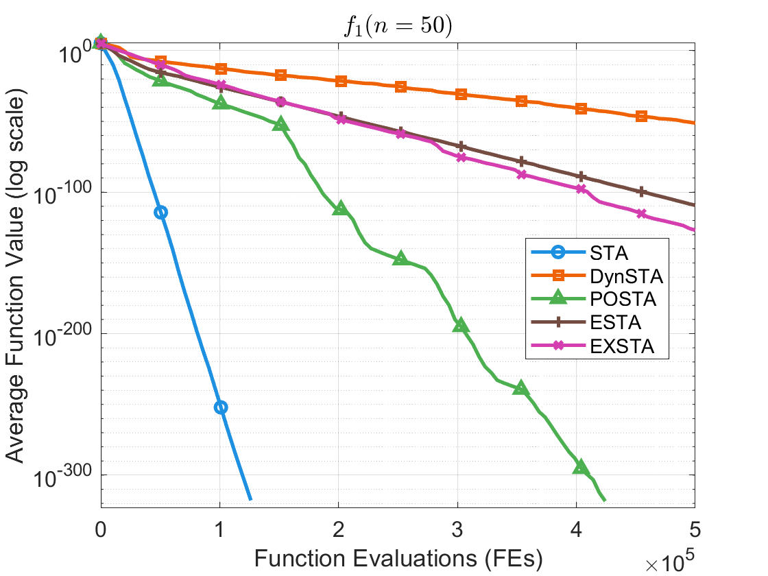
(a)

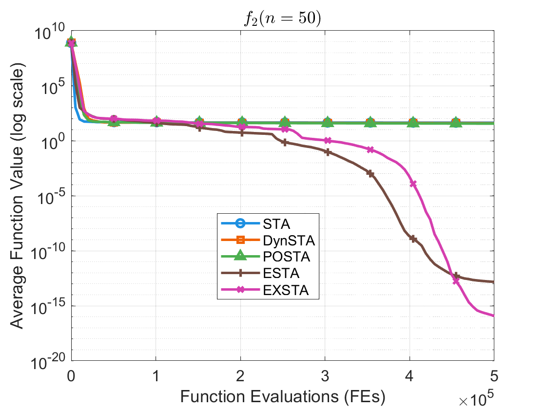
(b)

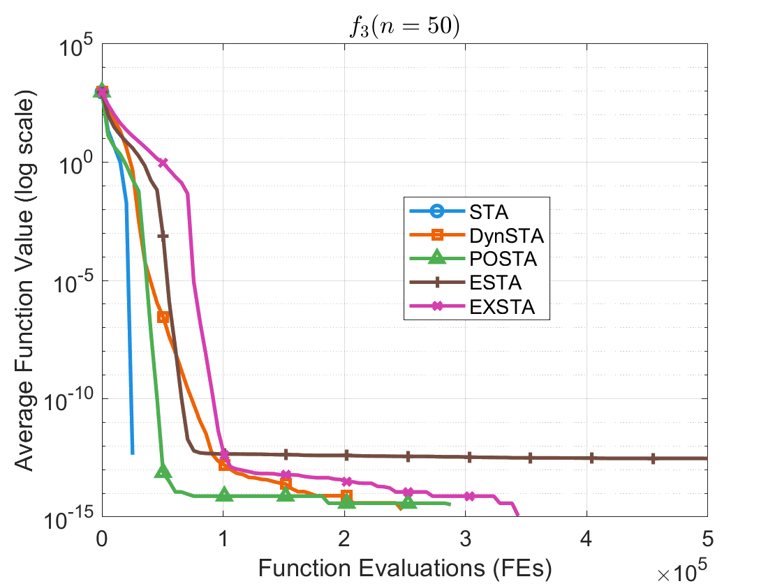
(c)

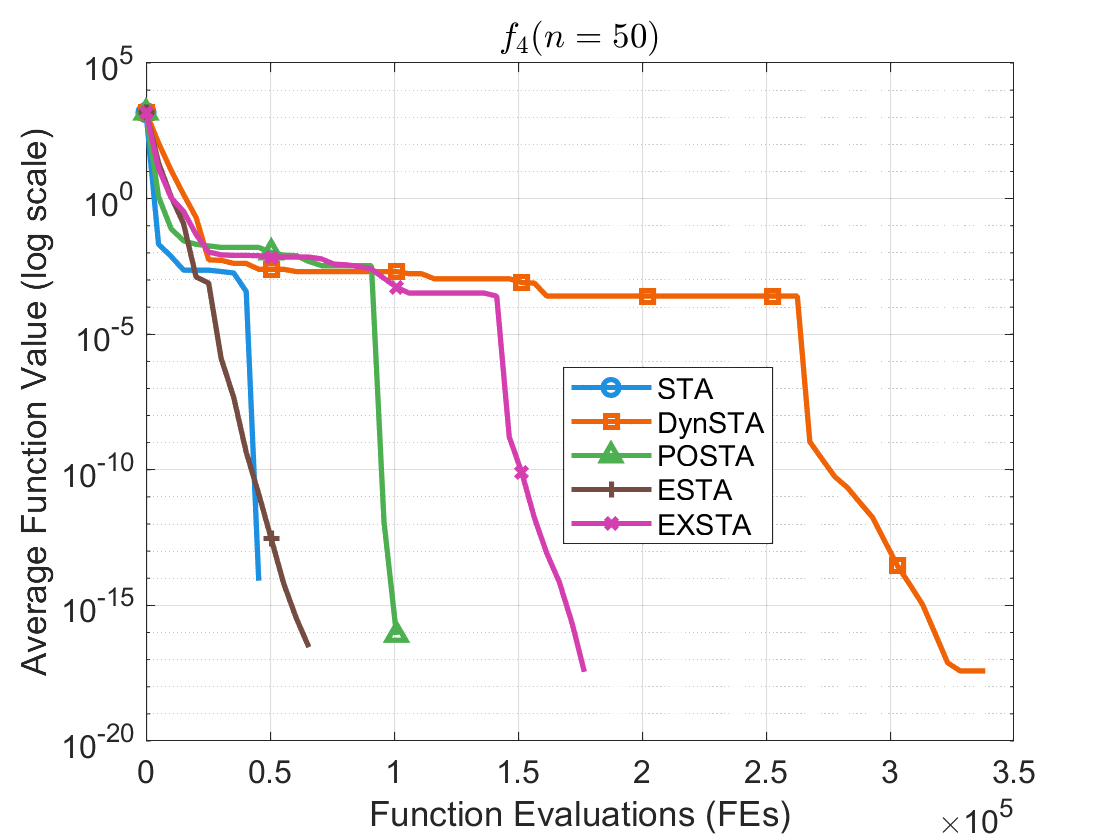
(d)

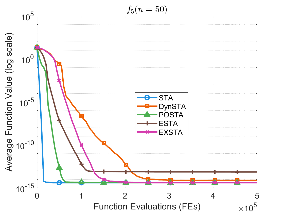
(e)

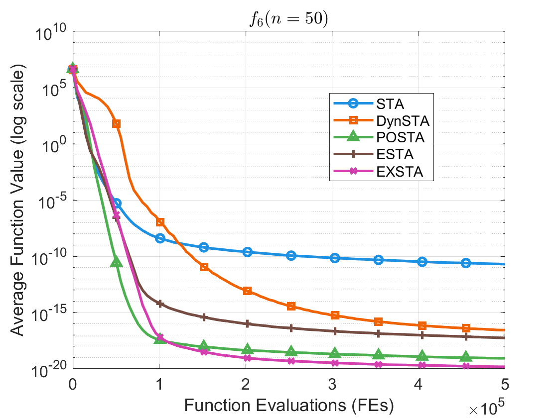
(f)

Figure 5: Iterative curves of STA variants for 50-dimensional problems

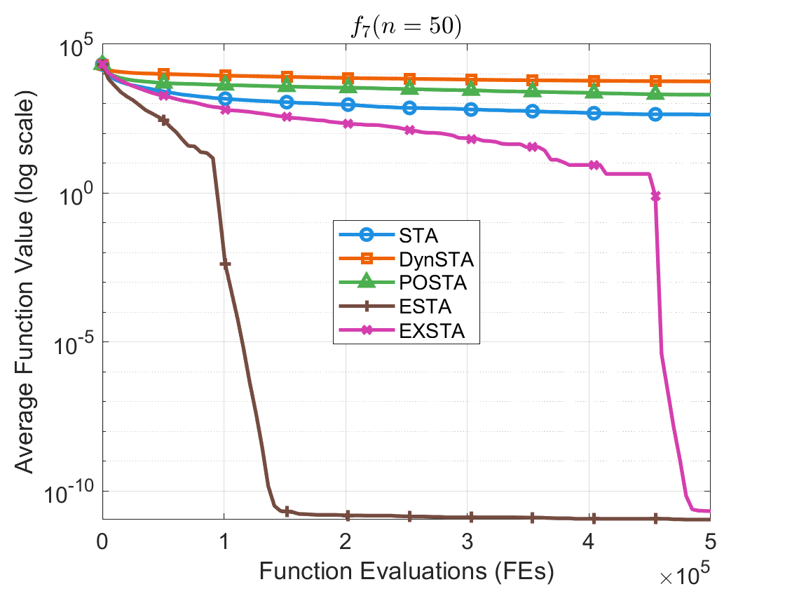
(g)

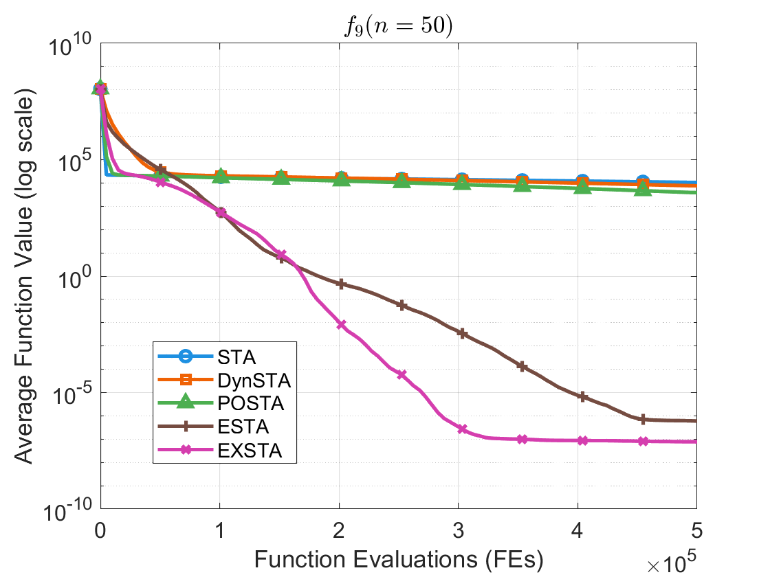
(h)

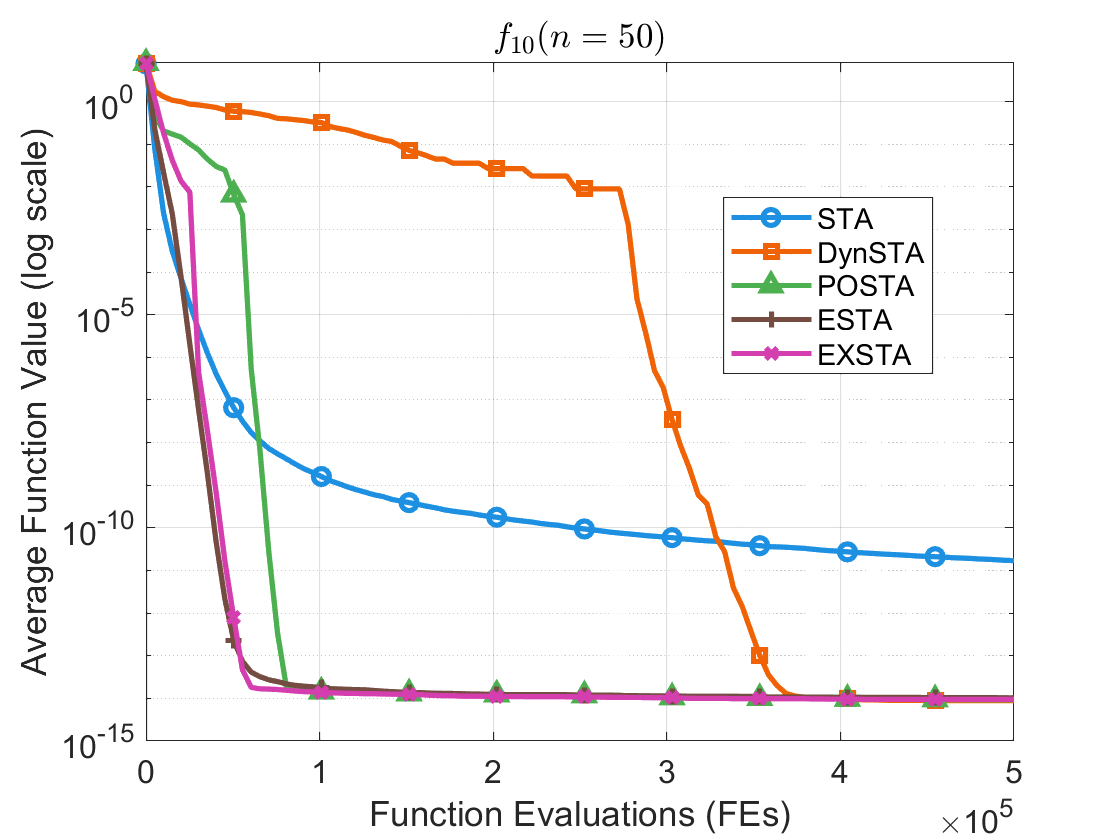
(i)

IV-D Comparison with other algorithms

In this subsection, the proposed effective STA is compared with other algorithms under two different termination criteria. The first criterion is the maximum number of stall iterations, which is used to assess whether the algorithm can guarantee convergence to an optimal solution. The second criterion is the maximum number of function evaluations, which is designed to evaluate the search capability of the algorithm.

IV-D1 Terminate at maximum stall iterations

In this part, the proposed method is compared with other algorithms under the termination condition of reaching the maximum number of stall iterations (maxStalls), which is set to maxStalls = 20. It is worth noting that the proposed method adopts its own designed termination condition, that is to say, in ESTA and EXSTA, maxStalls = 1. The average gradient norm (GradNorm) is shown in Table VI, with values greater than 1 highlighted in bold. It was found that with maxStalls = 1, the ESTA is able to guarantee an optimal solution. However, with maxStalls = 20, some algorithms are able to find the optimal solution for certain benchmark functions, but fail to do so for others. In other words, these algorithms cannot guarantee an optimal solution across all benchmark functions.

TABLE VI: Comparison of the average GradNorm with other algorithms under maxStalls

Fcn	Dim	GL25	CLPSO	CMAES	SaDE	GWO	WOA	HHO	SMA	ESTA
	20	3.17e+02	2.40e+02	0.00e+00	0.00e+00	0.00e+00	1.02e-02	2.66e-03	2.05e+00	5.11e-08
$f_{1}$	30	4.41e+02	3.80e+02	0.00e+00	0.00e+00	0.00e+00	9.46e-03	2.76e-03	9.95e-01	6.71e-08
	50	5.72e+02	6.08e+02	0.00e+00	0.00e+00	0.00e+00	1.58e-02	4.99e-03	1.80e+00	1.00e-07
	20	6.62e+06	3.29e+06	3.97e-07	1.38e+01	1.39e+01	6.71e+00	1.03e+01	4.53e+01	4.44e-06
$f_{2}$	30	1.05e+07	6.74e+06	5.69e-07	2.98e-07	1.55e+01	5.70e+00	1.37e+01	1.47e+03	6.36e-06
	50	1.48e+07	1.72e+07	8.37e-07	2.29e+01	1.76e+01	4.51e+00	1.67e+01	4.83e+02	9.82e-06
	20	1.85e+02	1.90e+02	1.57e+02	1.80e+02	5.55e+01	2.32e+00	6.27e-02	5.52e+01	1.23e-05
$f_{3}$	30	2.36e+02	2.34e+02	2.25e+02	2.00e+02	4.07e+01	3.01e+00	7.65e-02	5.75e+01	2.32e-05
	50	3.06e+02	3.01e+02	2.93e+02	3.04e+02	9.91e+01	2.39e-01	1.21e-01	6.04e+01	3.70e-05
	20	4.83e-01	3.77e-01	1.46e-02	9.89e-09	1.37e-02	2.01e-02	2.70e-03	1.20e-01	1.73e-08
$f_{4}$	30	6.66e-01	5.85e-01	1.07e-08	1.01e-08	1.40e-02	1.68e-02	1.52e-03	5.61e-02	1.89e-08
	50	8.66e-01	9.53e-01	1.06e-08	1.99e-02	9.64e-03	5.26e-03	2.60e-03	7.95e-02	2.30e-08
	20	1.14e+00	1.17e+00	9.80e-10	1.05e+00	1.12e-09	8.95e-01	8.84e-01	4.12e-01	1.15e-06
$f_{5}$	30	8.39e-01	9.64e-01	1.38e-09	1.07e+00	1.54e-09	7.38e-01	6.73e-01	3.82e-01	3.27e-06
	50	6.99e-01	7.20e-01	7.82e-08	8.07e-01	2.04e-09	5.71e-01	5.39e-01	4.08e-01	3.49e-06
	20	6.22e+02	4.76e+02	5.45e-16	3.69e-14	3.73e+01	1.54e+00	2.18e+01	7.51e+01	8.11e-08
$f_{6}$	30	1.34e+03	1.18e+03	4.58e-16	1.54e-13	7.86e+01	3.87e+00	5.95e+01	1.40e+02	1.13e-07
	50	2.93e+03	3.15e+03	3.73e-15	4.89e+01	2.33e+02	1.55e+01	1.65e+02	2.96e+02	2.03e-07
	20	2.47e+01	2.43e+01	2.25e+01	2.12e+01	2.44e+01	2.59e+00	1.02e+00	1.08e+01	2.97e-06
$f_{7}$	30	3.24e+01	3.10e+01	2.76e+01	2.25e+01	3.20e+01	4.10e+00	8.74e-01	1.26e+01	5.46e-06
	50	3.92e+01	3.95e+01	3.69e+01	3.36e+01	4.06e+01	5.18e+00	1.23e+00	1.58e+01	9.27e-06
	20	6.62e+01	7.10e+01	7.89e+01	6.48e+01	5.64e+01	4.06e+01	5.23e+01	6.23e+01	1.95e-05
$f_{8}$	30	9.70e+01	1.11e+02	1.36e+02	1.21e+02	9.57e+01	9.95e+01	1.06e+02	1.04e+02	5.69e-05
	50	2.38e+02	2.13e+02	2.50e+02	2.33e+02	2.12e+02	2.06e+02	2.27e+02	2.26e+02	2.03e-04
	20	1.31e+03	1.08e+03	1.62e-05	1.81e+01	2.19e+01	1.84e+00	2.02e+01	3.50e+01	4.14e-05
$f_{9}$	30	3.71e+03	3.66e+03	6.33e-05	4.57e-05	3.08e+01	5.72e+00	3.77e+01	6.14e+01	1.61e-04
	50	1.65e+04	1.73e+04	2.27e-02	2.53e+02	2.88e+01	2.90e+01	7.08e+01	1.15e+02	9.75e-04
	20	1.67e+00	1.60e+00	5.56e-08	3.56e-01	1.16e+00	3.86e-02	1.11e-02	3.33e-01	1.60e-07
$f_{10}$	30	2.23e+00	2.21e+00	8.98e-08	6.04e-01	1.71e+00	6.01e-02	1.45e-02	3.32e-01	3.17e-07
	50	2.89e+00	3.08e+00	1.48e-07	8.94e-01	2.44e+00	1.04e-01	1.37e-02	5.20e-01	4.34e-07

IV-D2 Terminate at maximum function evaluations

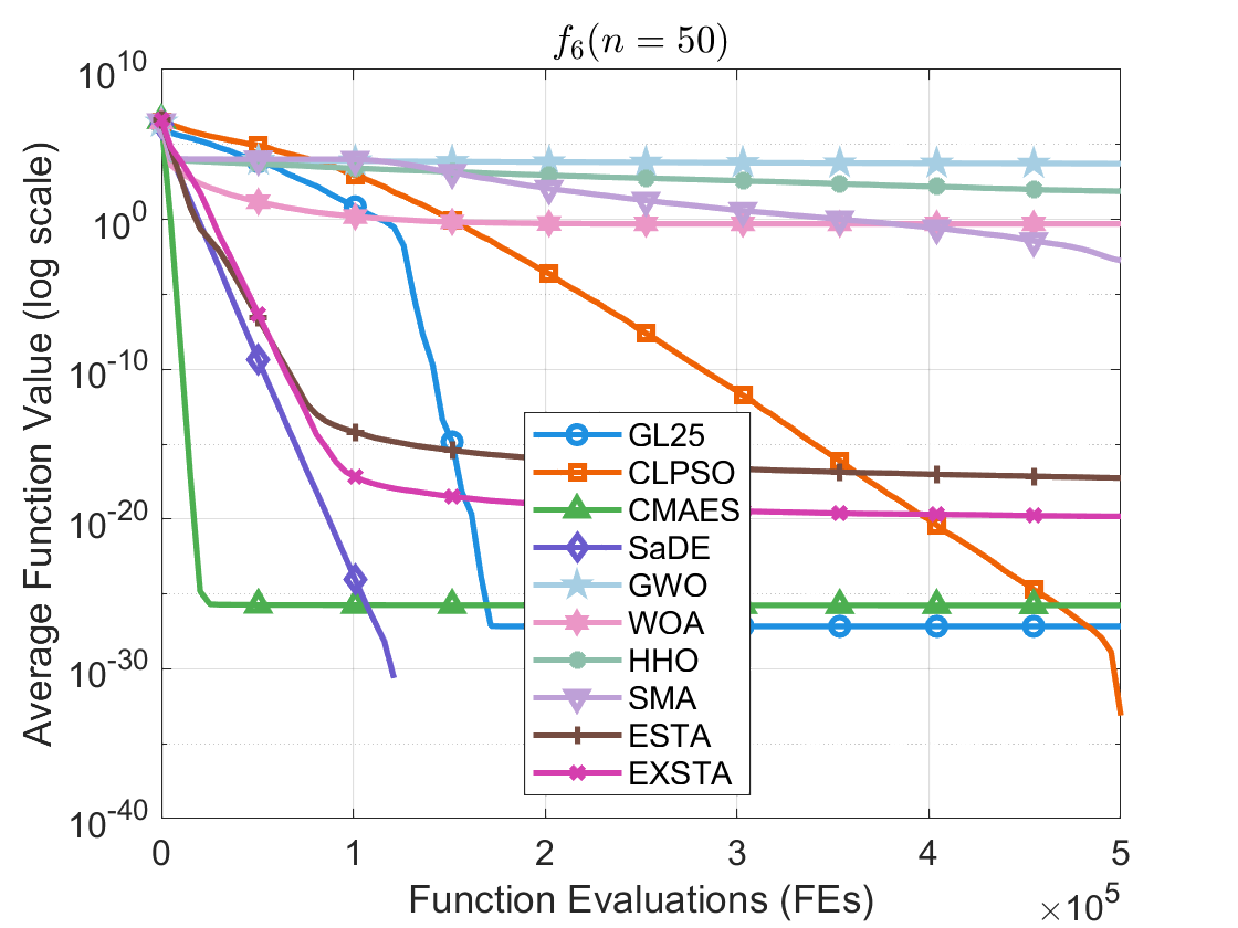
(f)

Figure 6: Comparison of iterative curves for the proposed algorithm and other algorithms on 50-dimensional problems

In this part, the proposed effective STA is compared with other algorithms under the maximum function evaluations (maxFEs), and the maxFEs is set to 1e4$n$. The statistical results are presented in Table VII and Table VIII, and the iterative curves for the 50-dimensional problems are illustrated in Fig. 6(f). For the benchmark functions with an all-zero optimal solution $(f_{1},f_{3},f_{4},f_{5})$, it is observed that the majority of optimization algorithms are able to find the global optimal solutions with high accuracy, especially for those recently popular methods. For the multimodal Rastrigin function, both GL25 and CMAES are prone to getting trapped in local minima. For the flattened Rosenbrock function, half of both well-established and recently popular methods have difficulty in accelerating the search process.

Then, the statistical results of the benchmark functions with an all-zero optimal solution are analyzed. For the Quadconvex function $f_{6}$ with a non-zero optimal solution and no other specific characteristics, an unusual phenomenon is observed for the recently popular methods, as they perform poorly on this convex optimization problem, while the well-established methods yield good results. The Trid function $f_{9}$ is also a convex optimization problem, but due to its flattened, nonseparable and nonidentical optimal-solution characteristics, the majority of algorithms perform poorly. For the multimodal Schwefel function $f_{7}$, GL25, CMAES and GWO are also prone to getting trapped in local minima. Almost all algorithms perform well on the Giunta function $f_{10}$ (with the exception of GWO) as the primary challenge in optimizing this function lies in its multimodality.

In general, the proposed ESTA and EXSTA exhibit excellent performance across nearly all benchmark functions (except the Griewank function in low dimensions) in handling challenges such as flat landscapes, nonseparability, multimodality, nonzero and nonidentical optima, especially on the Michalewicz function $f_{8}$ with an unknown global optimal solution, where they consistently find relatively better solutions. By the Wilcoxon rank-sum test, it is found that the proposed ESTA and EXSTA perform slightly worse to other algorithms on benchmark functions with an all-zero optimal solution $(f_{1},f_{3},f_{4},f_{5})$. That can be well explained by the fact that the solution accuracy is limited ($\epsilon=10^{-8}$) for ESTA and EXSTA in the experiments.

TABLE VII: Comparison of the average ObjVal with other algorithms under maxFEs

Fcn	Dim	GL25	CLPSO	CMAES	SaDE	GWO	WOA	HHO	SMA	ESTA	EXSTA
	20	6.42e-322	1.98e-30	0.00e+00	5.67e-130	0.00e+00	0.00e+00	0.00e+00	0.00e+00	2.57e-121	1.99e-209
$f_{1}$	30	8.82e-238	4.43e-30	0.00e+00	8.40e-139	0.00e+00	0.00e+00	0.00e+00	0.00e+00	9.89e-116	5.43e-196
	50	8.32e-172	3.71e-30	0.00e+00	5.78e-139	0.00e+00	0.00e+00	0.00e+00	0.00e+00	5.10e-110	1.23e-127
	20	1.13e+01	9.79e-01	2.20e-29	1.80e-29	1.62e+01	1.45e+01	1.83e-05	8.00e-04	3.07e-15	1.42e-17
$f_{2}$	30	2.09e+01	3.67e+00	3.25e-28	2.50e-17	2.64e+01	2.44e+01	1.52e-05	1.99e-03	1.64e-14	7.02e-17
	50	4.15e+01	1.17e+01	1.73e-27	8.53e-06	4.65e+01	4.39e+01	7.66e-06	3.56e-03	1.49e-13	1.19e-16
	20	1.07e+01	0.00e+00	4.80e+01	0.00e+00	0.00e+00	0.00e+00	0.00e+00	0.00e+00	0.00e+00	0.00e+00
$f_{3}$	30	2.32e+01	0.00e+00	5.24e+01	0.00e+00	0.00e+00	0.00e+00	0.00e+00	0.00e+00	1.14e-13	0.00e+00
	50	6.13e+01	0.00e+00	1.10e+02	0.00e+00	0.00e+00	0.00e+00	0.00e+00	0.00e+00	2.96e-13	0.00e+00
	20	6.24e-15	1.05e-16	0.00e+00	0.00e+00	0.00e+00	0.00e+00	0.00e+00	0.00e+00	8.31e-03	0.00e+00
$f_{4}$	30	1.50e-16	0.00e+00	0.00e+00	0.00e+00	0.00e+00	0.00e+00	0.00e+00	0.00e+00	0.00e+00	0.00e+00
	50	2.17e-15	0.00e+00	0.00e+00	0.00e+00	0.00e+00	0.00e+00	0.00e+00	0.00e+00	0.00e+00	0.00e+00
	20	1.19e-14	1.47e-14	1.95e+01	4.00e-15	4.00e-15	2.81e-15	4.44e-16	4.44e-16	2.69e-14	4.00e-15
$f_{5}$	30	3.44e-14	1.47e-14	1.94e+01	4.00e-15	7.55e-15	4.00e-15	4.44e-16	4.44e-16	4.12e-14	4.00e-15
	50	3.97e-13	2.18e-14	8.59e-02	6.68e-01	7.55e-15	4.44e-16	4.44e-16	4.44e-16	7.15e-14	4.00e-15
	20	0.00e+00	0.00e+00	4.67e-29	0.00e+00	4.55e+01	6.68e-03	3.97e+00	4.27e-04	1.06e-18	2.18e-23
$f_{6}$	30	7.54e-29	1.65e-30	1.14e-27	0.00e+00	5.87e+02	8.17e-02	1.50e+01	7.39e-04	2.86e-18	5.80e-22
	50	6.87e-28	7.70e-34	1.73e-26	0.00e+00	5.27e+03	5.04e-01	7.57e+01	1.76e-03	5.47e-18	1.48e-20
	20	1.67e+03	0.00e+00	3.48e+03	0.00e+00	3.77e+03	2.15e-02	1.27e-03	2.07e-04	1.82e-12	1.82e-12
$f_{7}$	30	3.43e+03	0.00e+00	5.21e+03	0.00e+00	6.26e+03	2.81e-02	5.89e-04	4.18e-04	1.82e-12	4.33e-12
	50	6.93e+03	3.64e-12	8.04e+03	0.00e+00	1.18e+04	2.58e-02	4.50e-04	7.21e-04	1.09e-11	2.10e-11
	20	-1.87e+01	-1.96e+01	-1.58e+01	-1.96e+01	-1.39e+01	-1.05e+01	-1.03e+01	-1.52e+01	-1.96e+01	-1.96e+01
$f_{8}$	30	-2.62e+01	-2.94e+01	-2.37e+01	-2.96e+01	-1.89e+01	-1.42e+01	-1.43e+01	-2.14e+01	-2.96e+01	-2.96e+01
	50	-2.87e+01	-4.85e+01	-3.86e+01	-4.83e+01	-2.86e+01	-2.10e+01	-2.11e+01	-3.33e+01	-4.96e+01	-4.96e+01
	20	3.64e+02	3.43e+02	-8.73e-11	6.06e-10	1.26e+03	1.43e+00	1.24e+01	8.67e+00	3.41e-10	3.01e-11
$f_{9}$	30	2.74e+03	3.55e+03	-5.82e-10	1.21e+01	4.64e+03	2.04e+01	1.93e+02	5.31e+02	1.12e-08	8.77e-10
	50	2.02e+04	4.67e+04	-3.73e-09	5.79e+03	2.18e+04	1.31e+03	3.73e+03	1.11e+04	5.98e-07	7.68e-08
	20	-1.78e-15	-1.78e-15	-1.78e-15	-1.78e-15	1.24e-07	2.38e-06	3.02e-08	9.89e-08	3.85e-16	-6.22e-16
$f_{10}$	30	0.00e+00	-3.55e-15	-3.55e-15	-3.55e-15	2.21e-01	4.01e-06	2.28e-08	2.35e-07	1.54e-15	1.95e-15
	50	1.07e-14	-1.78e-15	0.00e+00	-1.78e-15	9.53e-01	8.73e-06	9.93e-09	9.18e-08	1.02e-14	9.47e-15

TABLE VIII: Wilcoxon rank-sum test for other algorithms

Type	10D			30D			50D
	#+	#=	#-	#+	#=	#-	#+	#=	#-
GL25	2	0	8	2	1	7	2	1	7
CLPSO	2	1	7	2	2	6	3	2	5
CMAES	3	1	6	3	2	5	5	1	4
SaDE	4	3	3	4	3	3	3	3	4
GWO	1	3	6	1	2	7	1	2	7
WOA	2	2	6	1	3	6	2	2	6
HHO	2	2	6	2	2	6	2	2	6
SMA	2	2	6	2	2	6	2	2	6

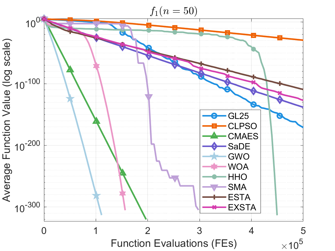
(a)

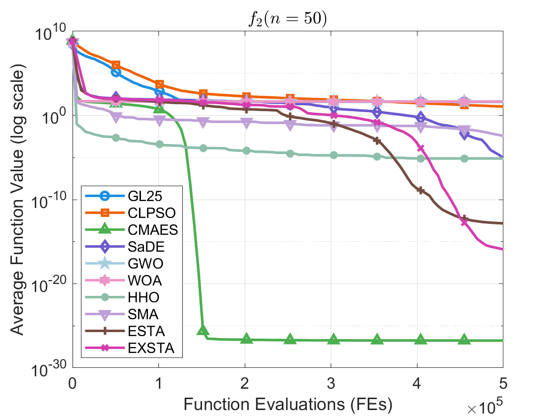
(b)

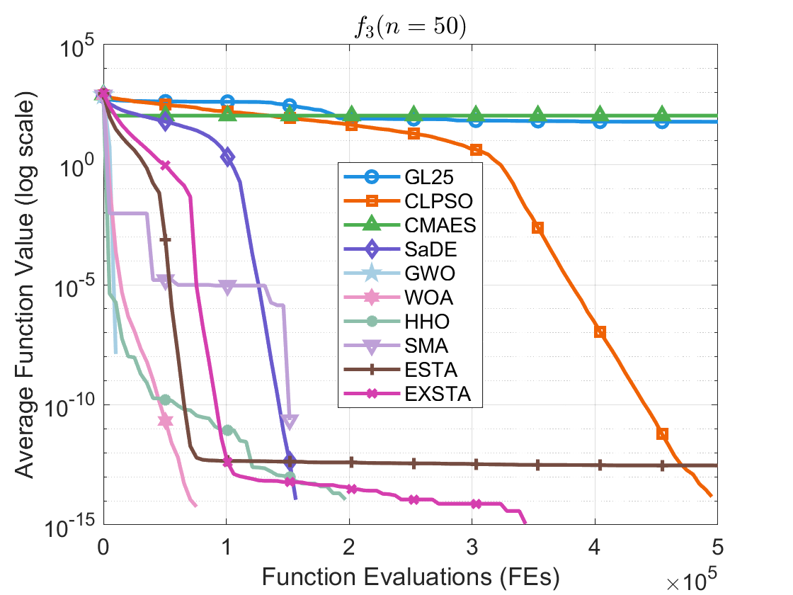
(c)

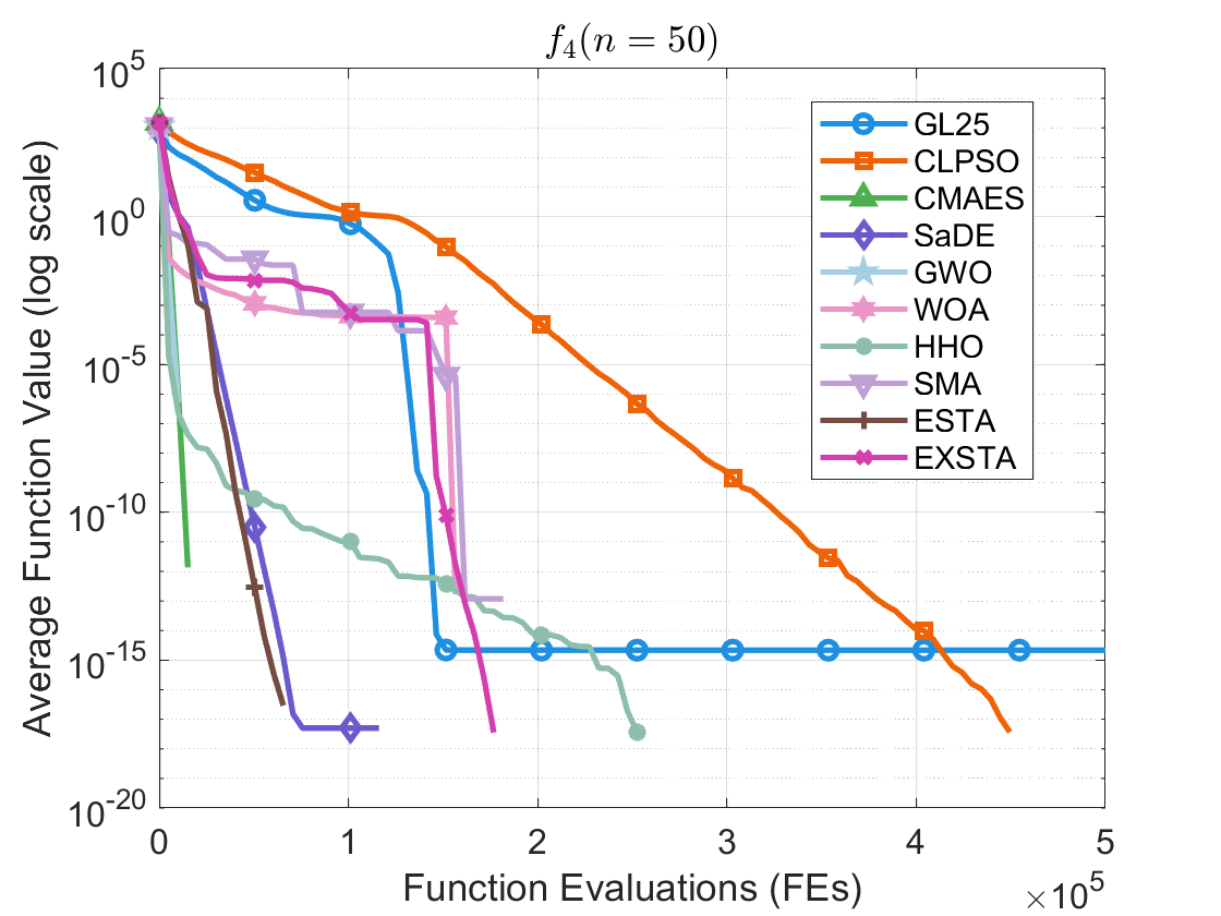
(d)

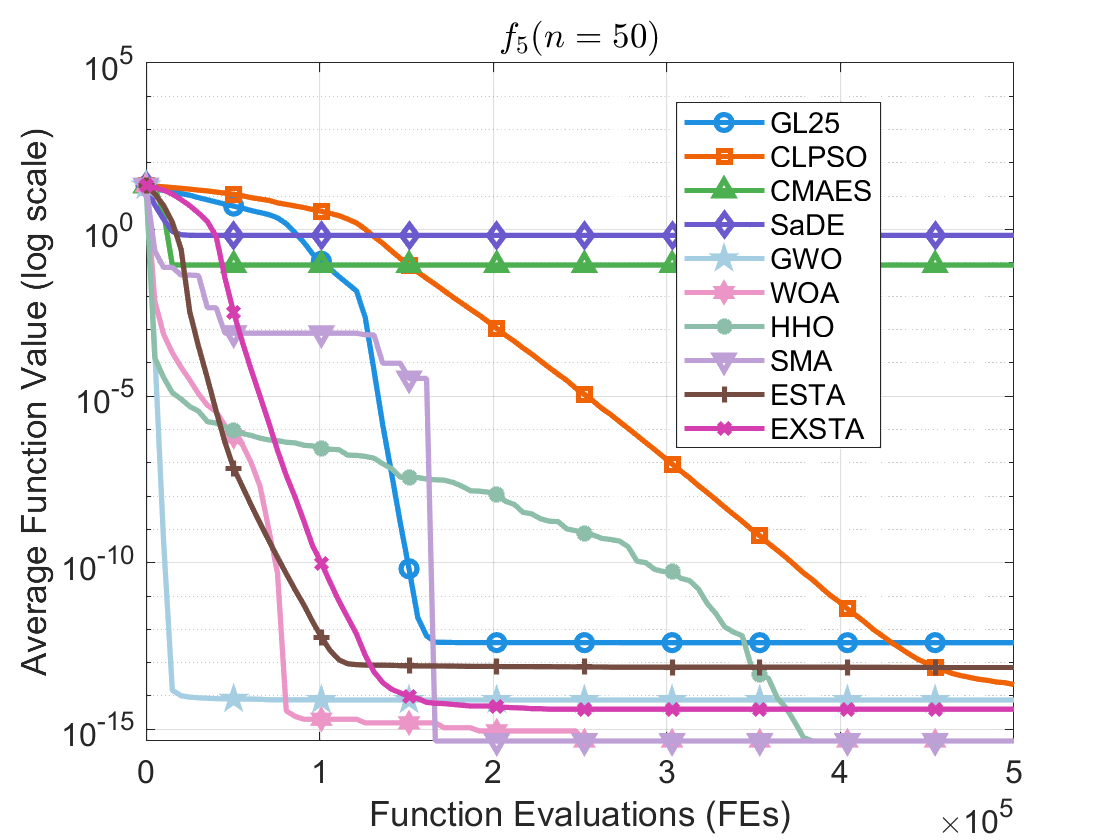
(e)

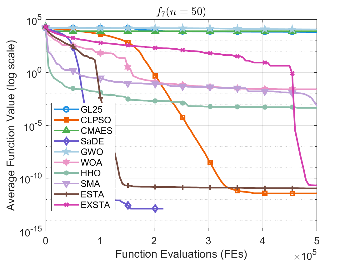
(g)

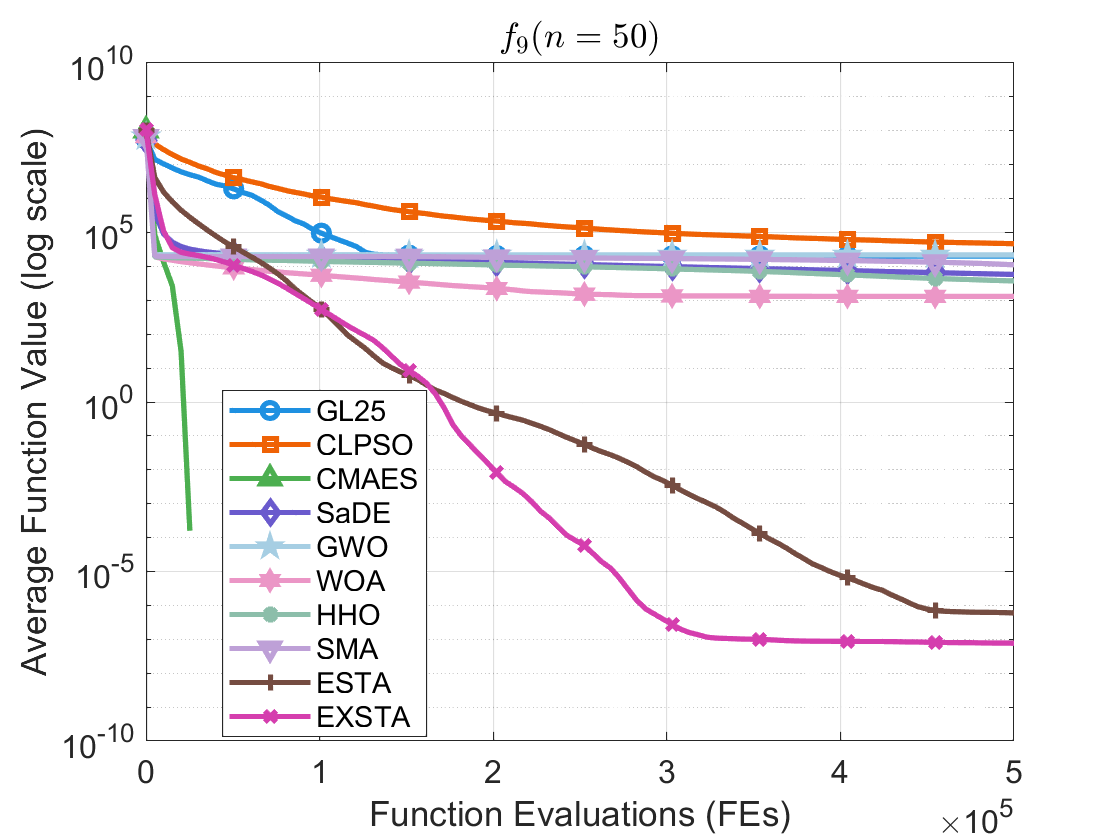
(h)

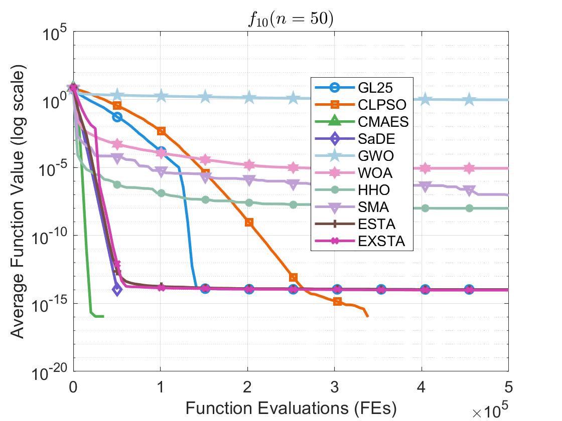
(i)

V Conclusion

In this study, an efficient STA with guaranteed optimality was proposed. First, novel translation transformations based on predictive models were introduced to generate more potential candidate solutions and accelerate convergence. Next, parameter control strategies were developed to enhance search efficiency. Finally, specific termination conditions were designed to ensure that the STA is capable of finding an optimal solution. Comparative analysis with other well-established and recently popular metaheuristics demonstrated the effectiveness of the proposed method. It is especially noteworthy that, given the small sample size (SE = 30), the proposed ESTA and EXSTA are capable of achieving truly optimal solutions.

It should be noted that the proposed ESTA occasionally performs suboptimally for the Griewank function in low dimensions, as the near-global solution in the Griewank function is located far from the true global solution. In such cases, the proposed ESTA faces difficulty in escaping local minima. Nevertheless, the proposed approach, along with the majority of existing studies on STA, primarily focuses on individual-based and sampling-based methods. In the future, population-based STA will be further explored to enhance its global search capabilities.

References

- [1] X. Zhou, C. Yang, and W. Gui, “A statistical study on parameter selection of operators in continuous state transition algorithm,” IEEE Transactions on Cybernetics, vol. 49, no. 10, pp. 3722–3730, 2019.
- [2] ——, “The principle of state transition algorithm and its applications,” Acta Automatica Sinica, vol. 46, no. 11, pp. 2260–2274, 2020.
- [3] J. Tang, G. Liu, and Q. Pan, “A review on representative swarm intelligence algorithms for solving optimization problems: Applications and trends,” IEEE/CAA Journal of Automatica Sinica, vol. 8, no. 10, pp. 1627–1643, 2021.
- [4] I. Supena, A. Darmuki, and A. Hariyadi, “The influence of 4c (constructive, critical, creativity, collaborative) learning model on students’ learning outcomes.” International Journal of Instruction, vol. 14, no. 3, pp. 873–892, 2021.
- [5] X. Zhou, C. Yang, and W. Gui, “State transition algorithm,” Journal of Industrial and Management Optimization, vol. 8, no. 4, pp. 1039–1056, 2012.
- [6] X. Zhou, X. Wang, T. Huang, and C. Yang, “Hybrid intelligence assisted sample average approximation method for chance constrained dynamic optimization,” IEEE Transactions on Industrial Informatics, vol. 17, no. 9, pp. 6409–6418, 2021.
- [7] J. Han, C. Yang, C.-C. Lim, X. Zhou, and P. Shi, “Stackelberg game approach for robust optimization with fuzzy variables,” IEEE Transactions on Fuzzy Systems, vol. 30, no. 1, pp. 258–269, 2022.
- [8] F. Lin, X. Zhou, C. Li, T. Huang, and C. Yang, “Data-driven state transition algorithm for fuzzy chance-constrained dynamic optimization,” IEEE Transactions on Neural Networks and Learning Systems, vol. 34, no. 9, pp. 5322–5331, 2023.
- [9] Y. Dong, C. Wang, H. Zhang, and X. Zhou, “A novel multi-objective optimization framework for optimal integrated energy system planning with demand response under multiple uncertainties,” Information Sciences, vol. 663, p. 120252, 2024.
- [10] X. Zhou, W. Tan, Y. Sun, T. Huang, and C. Yang, “Multi-objective optimization and decision making for integrated energy system using sta and fuzzy topsis,” Expert systems with applications, vol. 240, p. 122539, 2024.
- [11] X. Zhou, M. Li, Y. Du, C. Yang, and S. Wen, “Interpretable multiobjective feature selection via visualization in froth flotation process,” IEEE Transactions on Industrial Informatics, vol. 21, no. 3, pp. 2530–2539, 2025.
- [12] M. S. Bazaraa, H. D. Sherali, and C. M. Shetty, Nonlinear programming: theory and algorithms. John wiley & sons, 2006.
- [13] H. Aytug and G. J. Koehler, “New stopping criterion for genetic algorithms,” European Journal of Operational Research, vol. 126, no. 3, pp. 662–674, 2000.
- [14] S. N. Ghoreishi, A. Clausen, and B. N. Jørgensen, “Termination criteria in evolutionary algorithms: A survey.” in IJCCI, 2017, pp. 373–384.
- [15] Y. Liu, A. Zhou, and H. Zhang, “Termination detection strategies in evolutionary algorithms: a survey,” in Proceedings of the Genetic and Evolutionary Computation Conference, 2018, pp. 1063–1070.
- [16] S. Kukkonen and C. A. C. Coello, “A simple and effective termination condition for both single-and multi-objective evolutionary algorithms,” in 2019 IEEE Congress on Evolutionary Computation (CEC). IEEE, 2019, pp. 3053–3059.
- [17] L. Martí, J. García, A. Berlanga, and J. M. Molina, “A stopping criterion for multi-objective optimization evolutionary algorithms,” Information Sciences, vol. 367, pp. 700–718, 2016.
- [18] M. Ravber, S.-H. Liu, M. Mernik, and M. Črepinšek, “Maximum number of generations as a stopping criterion considered harmful,” Applied Soft Computing, vol. 128, p. 109478, 2022.
- [19] X. Zhou, P. Shi, C.-C. Lim, C. Yang, and W. Gui, “A dynamic state transition algorithm with application to sensor network localization,” Neurocomputing, vol. 273, pp. 237–250, 2018.
- [20] Y. Li, K. Wu, and J. Liu, “Self-paced ARIMA for robust time series prediction,” Knowledge-Based Systems, vol. 269, p. 110489, 2023.
- [21] G. P. Zhang, “Time series forecasting using a hybrid ARIMA and neural network model,” Neurocomputing, vol. 50, pp. 159–175, 2003.
- [22] C. García-Martínez, M. Lozano, F. Herrera, D. Molina, and A. M. Sánchez, “Global and local real-coded genetic algorithms based on parent-centric crossover operators,” European Journal of Operational Research, vol. 185, no. 3, pp. 1088–1113, 2008.
- [23] J. J. Liang, A. K. Qin, P. N. Suganthan, and S. Baskar, “Comprehensive learning particle swarm optimizer for global optimization of multimodal functions,” IEEE transactions on evolutionary computation, vol. 10, no. 3, pp. 281–295, 2006.
- [24] N. Hansen, S. D. Müller, and P. Koumoutsakos, “Reducing the time complexity of the derandomized evolution strategy with covariance matrix adaptation (cma-es),” Evolutionary computation, vol. 11, no. 1, pp. 1–18, 2003.
- [25] A. K. Qin, V. L. Huang, and P. N. Suganthan, “Differential evolution algorithm with strategy adaptation for global numerical optimization,” IEEE transactions on Evolutionary Computation, vol. 13, no. 2, pp. 398–417, 2009.
- [26] S. Mirjalili, S. M. Mirjalili, and A. Lewis, “Grey wolf optimizer,” Advances in engineering software, vol. 69, pp. 46–61, 2014.
- [27] S. Mirjalili and A. Lewis, “The whale optimization algorithm,” Advances in engineering software, vol. 95, pp. 51–67, 2016.
- [28] A. A. Heidari, S. Mirjalili, H. Faris, I. Aljarah, M. Mafarja, and H. Chen, “Harris hawks optimization: Algorithm and applications,” Future generation computer systems, vol. 97, pp. 849–872, 2019.
- [29] S. Li, H. Chen, M. Wang, A. A. Heidari, and S. Mirjalili, “Slime mould algorithm: A new method for stochastic optimization,” Future generation computer systems, vol. 111, pp. 300–323, 2020.