Pets: General Pattern Assisted Architecture
For Time Series Analysis

Abstract

Time series analysis has found widespread applications in areas such as weather forecasting, anomaly detection, and healthcare. However, real-world sequential data often exhibit a superimposed state of various fluctuation patterns, including hourly, daily, and monthly frequencies. Traditional decomposition techniques struggle to effectively disentangle these multiple fluctuation patterns from the seasonal components, making time series analysis challenging. Surpassing the existing multi-period decoupling paradigms, this paper introduces a novel perspective based on energy distribution within the temporal-spectrum space. By adaptively quantifying observed sequences into continuous frequency band intervals, the proposed approach reconstructs fluctuation patterns across diverse periods without relying on domain-specific prior knowledge. Building upon this innovative strategy, we propose Pets, an enhanced architecture that is adaptable to arbitrary model structures. Pets integrates a Fluctuation Pattern Assisted (FPA) module and a Context-Guided Mixture of Predictors (MoP). The FPA module facilitates information fusion among diverse fluctuation patterns by capturing their dependencies and progressively modeling these patterns as latent representations at each layer. Meanwhile, the MoP module leverages these compound pattern representations to guide and regulate the reconstruction of distinct fluctuations hierarchically. Pets achieves state-of-the-art performance across various tasks, including forecasting, imputation, anomaly detection, and classification, while demonstrating strong generalization and robustness.

1 Introduction

Time series analysis plays a pivotal role across numerous domains [49; 17], such as traffic planning [53; 70], encompassing healthcare diagnostics [26; 52], financial risk surveillance [12], and missing data imputation [19; 1]. These extensive applications necessitate the TS models to capture clear, precise, and universal compound fluctuation patterns from the input series and utilize them in various domains and task scenarios [39; 61].

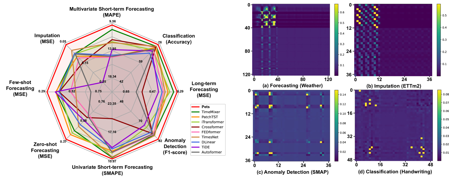
Figure 1: Pets demonstrates state-of-the-art performances on all 8 tasks (left). We visualize the attention score for diverse tasks (right). Specifically, The original sequence is decoupled into diverse fluctuation sequences, each undergoing the patch operation to yield a set of tokens. These three token sets are then combined, and attention score between any two tokens are calculated. For instance, in the forecasting task, the input series is decoupled into three fluctuation series, each yielding 40 tokens, and (a) shows the attention scores among the 120 tokens.

In recent years, the research endeavor of applying deep models to time series diverse tasks has achieved remarkable success [74; 75; 18]. Architectures meticulously designed based on fundamental backbone are regarded as the principal focus in time series investigations. Initial methods employed RNN [50; 3] and TCN [64; 55; 44] to capture the temporal dependency. Nevertheless, due to the limitations of Markov chains, RNNs tend to forget long-term dependency information. Meanwhile, TCNs have difficulty capturing global information owing to the constraints of the receptive field. Recently, models based on the transformer architecture [46; 43] have utilized the self-attention mechanism to establish global dependency among the observed sequences. Meanwhile, the lightweight MLP-based models [71; 67] have demonstrated outstanding potential in both the prediction preciseness and the computational complexity. Beyond these studies centered around modeling architectures, enhancement strategies based on time-frequency analysis assistance [76; 68; 69] and multi-scale algorithms [41; 40; 57; 56] have been integrated into time series analysis, with the focus on disentangling trends, seasonal or disparate scale components from the observed sequences. Nevertheless, in contrast to the tokens in language tasks that are strictly affiliated with distinct contexts [28], the isolated time point in time series manifests a superimposed state of multiple periodic-fluctuation patterns [57]. For instance, there exist disparate fluctuation modalities across three cyclical magnitudes: daily, monthly, and yearly. These limitations present significant obstacles for time series to comprehensively harness the inductive biases of the attention mechanism and convolution [56].

Our core motivation is employing the GPAs to improve the model’s capacity to discern and generalize universal patterns from observed sequences in a superimposed state. Decoupling observations of mixed multi-periodic series into a combination of multiple fluctuating modes will facilitate the adaptive selection of beneficial decomposition patterns for diverse downstream tasks. To illustrate the challenges in establishing GPA, Fig. 1 visualizes the attention scores between and within the decoupled fluctuation patterns under various tasks. Notably, the model tends to capture diverse pattern dependencies for specific downstream tasks. Specifically, for prediction and imputation tasks (Fig. 1 (a) and (b)), the model favors learning dependencies among low-frequency fluctuation tokens, and the intra-pattern score distribution shows periodical variation. In contrast, for anomaly detection and classification tasks (Fig. 1 (c) and (d)), the model is inclined to capture abrupt signals in high-frequency patterns for discriminative tasks. These impediments exemplify the challenges associated with constructing a flexible fluctuation pattern enhancement architecture that is universally applicable across a multiplicity of tasks and time series data.

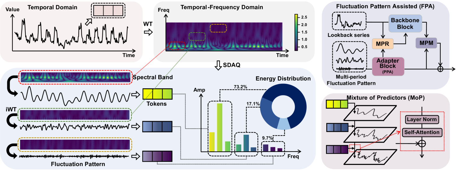
Figure 2: The overall architecture of Pets, which is based on the innovative temporal-spectral decomposition and amplitude quantization paradigm. Pets consists of features Fluctuation Pattern Assisted (FPA) and context-guided Mixture of Predictors (MoP), which respectively capture and aggregate the universal fluctuation patterns to enhance diverse tasks.

To address the inherent challenges of time series, this paper proposes Pets as a successful implementation of GPA, with the intention of learning the innate hybrid fluctuation pattern enhancement assemblages within time series by adaptively disentangling the dynamic superposition states of multiple period-fluctuation patterns. Its core design concept is to utilize a fixed spectrum distribution to guide the decoupling procedure, thereby establishing a residual-guided hybrid output paradigm by guaranteeing that the preponderant portion of time-frequency information and fluctuation energy is concentrated in particular fluctuation patterns. Concretely, the 1D observational sequence is disentangled and projected into the 2D time-frequency spectrum space. Thereafter, an Amplitude Margin Interval filter (AMI) is contrived to effectuate an adaptive partitioning of the spectral intervals, ensuring that the sequence projections within each interval exhibit a fixed spectrum distribution. This approach is designated by us as the Spectrum Decomposition and Amplitude Quantization strategy (SDAQ). Based on obtaining decoupled multiple Fluctuation patterns, we propose Fluctuation Pattern Assisted (FPA) consist of three components: (1) Periodic Prompt Adapter (PPA), (2) Multi-fluctuation Patterns Rendering (MPR), and (3) Multi-fluctuation Patterns Mixing (MPM) for the manipulation of the mixed periodic fluctuation modalities. Motivated by the periodic pattern interference mechanism [38], the PPA models the interaction factors among diverse fluctuations to uncover comprehensive temporal patterns. The MPR hierarchically aggregates these patterns and facilitates the backbone blocks in apprehending the hidden representations specific to certain patterns. The MPM promotes the renewal of compound fluctuation patterns and the capture of more profound hidden representations. In the generative scenario, such as prediction and imputation, we have proposed a context-guided mixture of predictors (MoP), which arranges the hidden representations of these fluctuations in descending order of energy proportion. Specifically, within the prediction task, the shallow predictor engenders the long-wave patterns of the future sequence, which subsequently functions as a conditional variable to guide the deep predictor in generating the short-wave patterns, thereby progressively constructing the predicted sequence. Our contributions can be summarized as:

• We propose Pets, a novel framework that disentangles the superimposed fluctuation patterns in time series from the energy-guided temporal-spectral decomposition perspective, enabling robust and interpretable time series decomposition for multiple downstream tasks.

• Pets incorporates three key components: PPA, MPR and MPM, to model the dependencies among fluctuation patterns and aggregate them effectively. These components enable the extraction of comprehensive temporal structures, the hierarchical learning of task-relevant features, and the refinement of mixed patterns, addressing the complexity of multi-pattern.

• Pets achieves state-of-the-art performances in all 8 mainstream time series analysis tasks across 60 benchmarks. Furthermore, Pets can consistently enhance the performance of disparate model architectures on extensive datasets and tasks.

2 Pets Architecture

In the long-term forecasting task, $X_{-L+1:0}\in\mathbb{R}^{B\times d\times L}$ and $X_{1:H}\in\mathbb{R}^{B\times d\times H}$ are utilized to represent the observed series and the future series, respectively, where $B$ denotes the batch size, $d$ denotes the number of channels of the multivariate time series, $L$ and $H$ denote the lookback window and forecast horizon. Based on the channel independent design, the input observation sequence $X_{-L+1:0}\in\mathbb{R}^{B\times d\times L}$ is first processed as $X_{-L+1:0}\in\mathbb{R}^{Bd\times L}$.

2.1 Decomposition and Quantization Paradigm

Temporal-Spectral Decomposition. Initially, through the application of the continuous wavelet transform (CWT) [34], the composite multi-periodic patterns inherent in the observed sequence $X_{-L+1:0}\in\mathbb{R}^{Bd\times L}$ are transmuted from the temporal space into biaxial space, yielding the temporal-frequency spectrum image $A\in\mathbb{R}^{Bd\times L\times\lambda}$, wherein $\lambda$ designates the spectral width within the time-frequency spectrum space. Specifically, we calculate the wave amplitude $A_{i,j}$ of the original sequence at time $t_{i}$ and frequency $f_{j}$, where $i\in[1,L],j\in[1,\lambda]$. This wave amplitude $A_{i,j}$ represents the magnitude of the observed sequence projected onto frequency band $f_{j}$ in the vicinity of time $t_{i}$, which is construed as the energy density of the observed sequence within the relevant fluctuation pattern. As shown in Fig. 2, in the time-frequency spectrum image, the light-colored blocks indicate the elevated wave amplitudes and energy densities at specified times and frequencies. Nevertheless, the spectral density distributions of time series data from diverse domains vary significantly, which causes the direct modeling on the image to limit the cross-domain generalization capacity of the model, and leads to substantial computational complexity. To address this issue, we propose a combined strategy of temporal-spectral decomposition and amplitude quantization.

Amplitude Quantization Phase. In the realm of prediction, the preponderant portion of high-energy density regions within the temporal-frequency spectrum is concentrated within the long-wave and low-frequency bands. This has inspired us to instigate the conception of the amplitude-margin interval (AMI). This paper aims to identify a relatively diminutive frequency domain interval (i.e., a frequency band) so that the preponderant amount of energy within the time-frequency domain space is involved within this band. The mathematical formulation of the AMI function is $\sum_{j\in[1,\textit{AMI}(\mu)]}\sum_{i\in[1,L]}A_{i,j}\textit{=}\mu\cdot\sum_{i}\sum_{j}A_{i,j},\mu\in(0,1)$, where $A_{:,j}\textit{=}\sum_{i\in[1,L]}A_{i,j}$ represents cumulative energy density of the spectrum $f_{j}$ over all time points. The function $\textit{AMI}(\mu)$ demarcates spectral interval $\{f_{j}\}_{1\leq j<\textit{AMI}(\mu),j\in\mathbb{Z}}$ such that a specific proportion of energy is located within this band. Consequently, a set of fixed proportions $\{\mu_{1},\mu_{2},..,\mu_{K\textit{-}1}\}$ can adaptively determine the partitioning of spectral sub-bands $sub_{1}\textit{=}\{f_{j}\}_{1\leq j<\textit{AMI}(\mu_{1})}$, $sub_{2}\textit{=}\{f_{j}\}_{\textit{AMI}(\mu_{1})\leq j<\textit{AMI}(\mu_{2})}$ and $sub_{K}\textit{=}\{f_{j}\}_{\textit{AMI}(\mu_{K\textit{-}1})\leq j<\lambda}$. Subsequently, $A\in\mathbb{R}^{Bd\times L\times\lambda}$ is deconstructed into $K$ time-frequency sub-images $A^{1,2,..,K}\in\mathbb{R}^{Bd\times L\times\lambda}$, Where $A^{k}$ is generated from $A$ by mask operation, ${A_{i,j}^{k}\textit{=}A_{i,j}~if~f_{j}\in sub_{k}~else~0}$, where $k\textit{=}1,2,..,K$. Ultimately, the inverse wavelet transform (iWT) is employed to project the three time-frequency spectrum images back into the time domain space, thereby realizing the spectrum decomposition and amplitude quantization process of the composite fluctuation pattern. And the decoupled sequences are defined as $X_{-L+1:0}^{k}\textit{=}iWT(A^{k})\in\mathbb{R}^{Bd\times L}$, where $k\textit{=}1,2,..,K$. The auxiliary quantization strategy adaptively segregates the complex and variable continuous spectrum into multiple spectrum intervals. We guarantee the scalability and generalization of the modeling by fixing the energy density distribution of the spectrum intervals. In our experiments, we keep the $(K\textit{=}3,\lambda\textit{=}50,\mu_{1}\textit{=}0.7,\mu_{2}\textit{=}0.9)$ setting, and we discuss the diverse hyperparameters in the Section D.3.

2.2 Patch Embedding

Following the patching instance strategy [46], each sequence of length $L$ is rerepresented as $P_{L}\times p$, where $p$ as the patch length, $P_{L}$ is the number of tokens, and satisfies $P_{L}\times p=L$. Based on this, the observation sequence $X_{-L+1:0}\in\mathbb{R}^{Bd\times L}$ and decoupled multi-periodic sequences $\{X_{-L+1:0}^{k}\in\mathbb{R}^{Bd\times L}\}_{k\in[1,K]}$ are converted as embedding $X_{-L+1:0}\in\mathbb{R}^{Bd\times P_{L}\times p}$ and $\{X_{-L+1:0}^{k}\in\mathbb{R}^{Bd\times P_{L}\times p}\}_{k\in[1,K]}$, where $P_{d}$ represents the dimension of tokens. Subsequently, observation tokens $E^{0}\in\mathbb{R}^{Bd\times P_{L}\times P_{d}}$ and multi-periodic tokens $\{E_{k}^{0}\in\mathbb{R}^{Bd\times P_{L}\times P_{d}}\}_{k\in[1,K]}$ are calculated by the embedding layer based on 1D convolution.

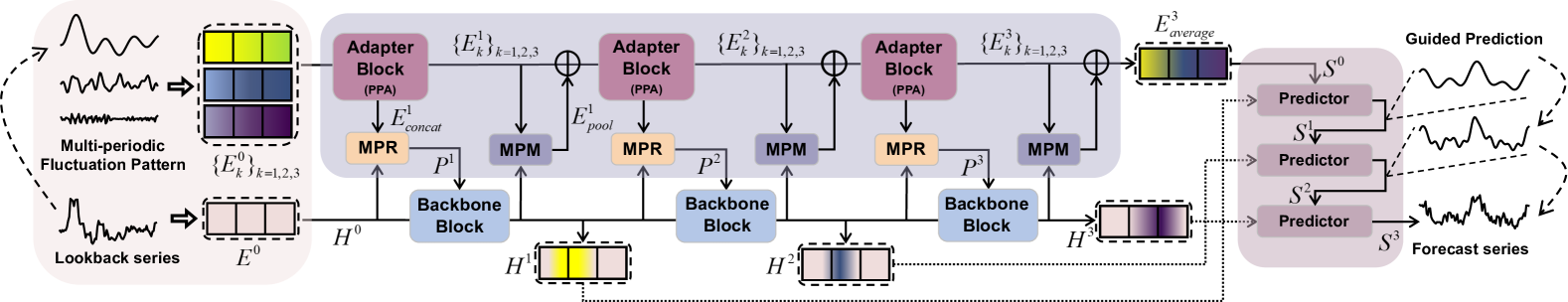
Figure 3: The overall architecture of Pets. Pets is a two-branch architecture consisting of three components: (a) a plain Transformer or MLP (Backbone Block), which is evenly divided into diverse stages for feature interaction. (b) FPA employs the proposed PPA (Adapter Block), MPR and MPM, to capture the dependencies between different fluctuation patterns, and (c) MoP adaptively aggregates the mixed fluctuation patterns according to the energy ranking order, and the fluctuation patterns with high task relevance can dominate the output. See Fig. 6 for detailed designs of PPA, MPR and MPM.

2.3 Periodic Pattern Interference Mechanism

The overall architecture of Pets is illustrated in Fig. 2 and comprises three components: (a) the common Transformer or MLP backbone. (b) the stacked Fluctuation Pattern Assisted (FPA), which assimilates the proposed Periodic Prompt Adapter (PPA), Multi-Fluctuation Patterns Rendering (MPR), and Multi-Fluctuation Patterns Mixing (MPM). (c) Mixture of Predictors (MoP). During the forward pass, the PPA and the backbone block respectively receive the composite fluctuation pattern embedding and the observed sequence embedding as inputs respectively. The PPA is employed to fortify the fluctuation pattern information. Subsequently, the MPR and MPM are devised to interact and fuse the bidirectional features between the two principal line. Finally, the MoP adaptively aggregates the fluctuation patterns, permitting the task highly relevant fluctuation patterns to dominate the model’s output. The proposed components can be facilely integrated into any advanced models (such as DLinear [71], PatchTST [46] and TimeMixer [57]) and consistently demonstrate state-of-the-art performance across diverse downstream tasks.

Periodic Prompt Adapter Blocks. PPA introduces composite fluctuation pattern information through bidirectional interaction to enhance the generalization capacity and semantic representation of the deep model while remaining adaptable to any fundamental architecture. Specifically, the adapter block at the $n$-th layer ($n\in[1,N]$) receives the representations of diverse patterns $\{E_{k}^{n-1}\in\mathbb{R}^{B\cdot d\times P_{L}\times P_{d}}\}_{k\in[1,K]}$ as inputs, and fully exploits the inductive bias of local convolution modeling to distill the deep characterizations under each periodic pattern from the input multi-periodic pattern embedding tokens: $E_{k}^{n-1}\textit{=}Conv1D(Linear(E_{k}^{n-1})^{\top})^{\top}$, and then $E_{k}^{n-1}\textit{=}Dropout(Linear(Act(E_{k}^{n-1})))$.

Subsequently, a self-attention layer is meticulously contrived with the intention of capturing the dependencies among disparate representations of various periodic fluctuation patterns, thereby empowering the model with an enhanced capacity to capture the composite temporal information. We commence by splicing $\{E_{k}^{n-1}\in\mathbb{R}^{B\cdot d\times P_{L}\times P_{d}}\}_{k\in[1,K]}$ along the dimension of the number of tokens to obtain $E_{concat}^{n-1}\in\mathbb{R}^{B\cdot d\times KP_{L}\times P_{d}}$, which as the concatenated mixed fluctuation pattern embedding. The self-attention mechanism is formulated as, $E_{concat}^{n-1}\textit{+=}SelfAttn(E_{concat}^{n-1})$, and then $E_{concat}^{n-1}\textit{+=}Conv1D(E_{concat}^{n-1})$. Finally, the mixed pattern representation independently executes three one-dimensional convolutions to decouple into embeddings $\{E_{k}^{n}\}_{k\in[1,K]}$ corresponding to multiple different fluctuation patterns, among which $E_{k}^{n}\textit{=}Conv1D_{k}(E_{concat}^{n-1})_{k\in[1,K]}$.

Multi-fluctuation Patterns Rendering. MPR augments the fluctuation patterns captured by the adapter block as conditional context to guide the backbone block to focus on modeling that particular fluctuation pattern. Concretely, the MPR module takes in two input tensors: the decoupled fluctuation pattern group $\{E_{k}^{n}\in\mathbb{R}^{B\cdot d\times P_{L}\times P_{d}}\}_{k\in[1,K]}$ outputted by the current layer’s adapter block and the hidden representation $H^{n-1}\in\mathbb{R}^{B\cdot d\times P_{L}\times P_{d}}$ generated by the previous layer’s backbone block (for the first MPR module, it is the embedding $E^{0}\in\mathbb{R}^{B\cdot d\times P_{L}\times P_{d}}$ of the observed sequence). During the forward progression, the distinctive zero-convolution design ensures that the MPRs is inclined to learn inductive biases from diverse fluctuation patterns. Specifically, within the shallow MPR block, the high-frequency pattern $\{E_{k}^{n}\}_{k\in[2,K]}$ undergoes a $1\times 1$ convolution with both weights and biases initialized to zero, and then is concatenated with the low-frequency pattern $\{E_{k}^{n}\}_{k=1}$ into the mixed fluctuation pattern tokens $E_{concat}^{n}$. Subsequently, similarly through the self-attention mechanism, and finally through the pooling layer, it is combined with the hidden representation $H^{n-1}$ via element-wise addition as the prompt embedding $P^{n}\in\mathbb{R}^{B\cdot d\times P_{L}\times P_{d}}$ of the current MPR layer. The mathematical formulation is expressed as: $E_{concat}^{n}\textit{+=}SelfAttn(E_{concat}^{n})$, $E_{concat}^{n}\textit{+=}Conv1D(E_{concat}^{n})$, and $P^{n}~\textit{=}~H^{n-1}\textit{+}Pool(E_{concat}^{n})$.

Backbone Blocks. In alignment with the design of popular baselines, to ascertain that the proposed Pets serves as a universal and plug-and-play enhanced architecture. When PatchTST is selected as the Backbone, the hidden representation $H^{n-1}\in\mathbb{R}^{B\cdot d\times P_{L}\times P_{d}}$ generates by the previous layer’s backbone block (for the first backbone block, it is the embedding $E^{0}\in\mathbb{R}^{B\cdot d\times P_{L}\times P_{d}}$ of the observed sequence) first passes through the transformer layer, and subsequently performs the element-wise addition operation with $P^{n}\in\mathbb{R}^{B\cdot d\times P_{L}\times P_{d}}$ calculated by the current layer’s MPR. The formula is as follows: $H^{n-1}\textit{+=}SelfAttn(H^{n-1})$ and $H^{n}\textit{=}P^{n}\textit{+}H^{n-1}\textit{+}FFN(H^{n-1})$.

Multi-fluctuation Patterns Mixing. The MPM module is meticulously contrived to ensure that the modeling results of the shallow backbone block regarding the prediction sequence are present within the hidden representations and are accessible to the deeper adapter block, as a result, significantly enhancing the generalization and performance of Pets to a great extent. MPM accepts two segments of inputs, namely a set of fluctuation pattern $\{E_{k}^{n}\in\mathbb{R}^{B\cdot d\times P_{L}\times P_{d}}\}_{k\in[1,K]}$ generated by the current layer’s adapter block and the hidden representation $H^{n}\in\mathbb{R}^{B\cdot d\times P_{L}\times P_{d}}$ generated by the current layer’s backbone block, and obtains the input for the next layer’s adapter block after forward progression. The MPM module first performs element-wise addition between the hidden representation and each fluctuation pattern representation, subsequently concatenating them together after independently passing through a convolution layer, $E_{k}^{n}\textit{=}Conv1D(E_{k}^{n}\textit{+}H^{n})$ and $E_{concat}^{n}\textit{=}Concatenate(\{E_{k}^{n}\}_{k\in[1,K]})$. Eventually, the attention is utilized to capture the dependencies among the mixed tokens of all multiple fluctuation patterns. After passing through the pooling layer, the updated pattern representation is obtained by $E_{pool}\textit{=}Pool(E_{concat}^{n}\textit{+}Conv1D(E_{concat}^{n})))$, which is employed to guide the generation of the fluctuation pattern of the next layer, as $\{E_{k}^{n}\textit{=}E_{k}^{n}\textit{+}E_{pool}^{n}\}_{k\in[1,K]}$.

Mixture of Predictors. In the forward procedure, the output result $\{E_{k}^{N}\in\mathbb{R}^{B\cdot d\times P_{L}\times P_{d}}\}_{k\in[1,K]}$ of the last MPM module is obtained by element-wise addition to yield $E_{average}^{N}\in\mathbb{R}^{B\cdot d\times P_{L}\times P_{d}}$. The intermediate result generated by the $n$-th backbone block is designated as the hidden representation group $\{H^{n}\in\mathbb{R}^{B\cdot d\times P_{L}\times P_{d}}\}_{n=1,2,...,N}$. To fortify the robustness and predictive performance of the model, Pets devises a innovative stepwise prediction strategy and a hybrid predictor architecture. In the MoP consisting of $N$ weight-independent predictors, each predictor receives two inputs. The dotted and solid lines symbolize reference tokens and situational tokens respectively, as depicted at the rightmost side in Fig. 2. The hidden representation $H^{n}$ serves as the reference tokens for the $n$-th predictor, with the first predictor receiving $E_{average}^{N}$ as the situational tokens. Furthermore, the output result of the n-th predictor is adopted as the previous tokens $S^{n\textit{+}1}$ for the (n+1)-th predictor.

Specifically, in the $n$-th predictor, we have $S^{n}\textit{+=}Selfattn(Conv1D(S^{n}))$, and the Element-wise Addition is performed between the situational tokens and the reference tokens, as follows $S^{n}\textit{+=}H^{n}\textit{+}FFN(S^{n})$ and $S^{n\textit{+}1}\textit{=}Conv1D(S^{n})$. The reference tokens $S^{N}\in\mathbb{R}^{B\cdot d\times P_{L}\times P_{d}}$ generated by the final predictor are flattened and then passed through a linear-based projection layer, thus obtaining the prediction result $\overline{X}_{1:H}~\textit{=}~OutputHead(Flatten(S^{N}))$.

3 Experiments

In order to validate the efficacy of the proposed Pets functioning as a general fluctuation pattern assist architecture, we conduct comprehensive experiments covering 8 popular temporal analytical scenarios. These encompass (1) long-term forecasting, (2) univariate and (3) multivariate short-term forecasting, (4) imputation, (5) classification, (6) anomaly detection, as well as (7) few-shot and (8) zero-shot forecasting. Collectively, as encapsulated in Figure 1, PETs invariably outperforms contemporary state-of-the-art across time series analytical tasks. The meticulous experimental setups and implementation details are provided in Appendix B.

Table 1: Comparison of the performance on Full Shot Forecasting task. We present the model’s average performance across multiple prediction horizons for each dataset and boldface the best performance. The detailed results are presented in Table 12.

Models	Pets		TimeMixer		iTransformer		PatchTST		Crossformer		TiDE		TimesNet		DLinear		SCINet		FEDformer
	(Ours)		[2024b]		[2024]		[2023]		[2021]		[2023]		[2023]		[2023]		[2021a]		[2022a]
Metric	MSE	MAE	MSE	MAE	MSE	MAE	MSE	MAE	MSE	MAE	MSE	MAE	MSE	MAE	MSE	MAE	MSE	MAE	MSE	MAE
Weather	0.219	0.255	0.240	0.271	0.258	0.278	0.265	0.285	0.264	0.320	0.271	0.320	0.259	0.287	0.265	0.315	0.292	0.363	0.309	0.360
Solar-Energy	0.187	0.244	0.216	0.280	0.233	0.262	0.287	0.333	0.406	0.442	0.347	0.417	0.403	0.374	0.330	0.401	0.282	0.375	0.328	0.383
Electricity	0.173	0.264	0.182	0.272	0.178	0.270	0.216	0.318	0.244	0.334	0.251	0.344	0.192	0.304	0.225	0.319	0.268	0.365	0.214	0.327
Traffic	0.403	0.269	0.484	0.297	0.428	0.282	0.529	0.341	0.667	0.426	0.760	0.473	0.620	0.336	0.625	0.383	0.804	0.509	0.610	0.376
ETTh1	0.415	0.426	0.447	0.440	0.454	0.447	0.516	0.484	0.529	0.522	0.541	0.507	0.458	0.450	0.461	0.457	0.747	0.647	0.498	0.484
ETTh2	0.360	0.398	0.364	0.395	0.383	0.407	0.391	0.411	0.942	0.684	0.611	0.550	0.414	0.427	0.563	0.519	0.954	0.723	0.437	0.449
ETTm1	0.351	0.382	0.381	0.395	0.407	0.410	0.406	0.407	0.513	0.495	0.419	0.419	0.400	0.406	0.404	0.408	0.485	0.481	0.448	0.452
ETTm2	0.255	0.310	0.275	0.323	0.288	0.332	0.290	0.334	0.757	0.610	0.358	0.404	0.291	0.333	0.354	0.402	0.954	0.723	0.305	0.349

3.1 Long-term Forecasting

Setups. Long-term forecasting emerges as a cornerstone for strategic scheming in arenas like traffic governance and energy exploitation. To conduct a thoroughgoing evaluation of our model, a battery of experiments is executed on 8 ubiquitously-employed real-world datasets, incorporating those related to Weather and Solar-Energy. These tasks conform to the precedent benchmarks established by  [75; 62; 40], thus guaranteeing comparability and relevance throughout our research undertakings.

Results. Table 1 shows Pets outperforms other models in long-term forecasting across various datasets. The MSE of Pets is reduced by 8.7% and 15.1% compared to the TimeMixer and iTransformer, respectively. For ETT (Avg), Pets achieves 7.4% lower MSE than TimeMixer. Specifically, it outperforms the runner-up model by a margin of 13.4% and 19.7% on the challenging Solar-Energy.

3.2 Short-term Forecasting

Table 2: Comparison of the performance on Short-term Forecasting task. The detailed results are presented in Table 15,  16.

Models		Pets	TimeMixer	iTrans.	TiDE	TimesNet	PatchTST	MICN	DLinear	FED.
		(Ours)	[2024b]	[2024]	[2023]	[2023]	[2023]	[2023]	[2023]	[2022a]
M4	SMAPE	11.568	11.723	12.684	13.950	11.829	13.152	19.638	13.639	12.840
	MASE	1.471	1.559	1.764	1.940	1.585	1.945	5.947	2.095	1.701
	OWA	0.834	0.840	0.929	1.020	0.851	0.998	2.279	1.051	0.918
PEMS	MAE	16.03	17.41	19.87	21.86	20.54	23.01	19.34	23.31	23.50
	MAPE	9.99	10.59	12.54	13.80	12.69	14.94	12.38	14.68	15.01
	RMSE	26.11	28.01	31.29	34.42	33.24	36.05	30.40	37.32	36.78

Setups. Short-term forecasting assumes a critical function within the purview of financial decision-making and market risk evaluation tasks. To appraise the performance under both univariate and multivariate configurations, we utilize the M4 Competition dataset [45] and the PeMS dataset [9] as benchmarks. In where, the M4 dataset comprises a hundred thousand marketing time steps, whereas the PeMS dataset incorporates four high-dimensional traffic network datasets. These comprehensive benchmarks furnish a formidable evaluating platform for an assessment of the model’s efficacy.

Results. The results enumerated in Table 2 manifest the state-of-the-art performance of Pets within all short-term forecasting benchmarks. In the M4 dataset, compared to the challenging TimeMixer and TimesNet, Pets accomplishes a reduction of 5.6% and 7.2% in MASE, respectively. Within the PEMS, in comparison to the leading TimeMixer and iTransformer, Pets reduces MAPE by 5.7% and 20.3%. Remarkably, in comparison with the conventional PatchTST, Pets exhibits performance augmentations on M4 and PEMS that exceed 24.4% and 33.1% respectively.

3.3 Imputation

The endeavor of imputing missing values profound significance for time series analysis. For instance, its pivotal role in rectifying the absent values extant in wearable sensors. To appraise the imputation capabilities of our model, the left of table 3 demonstrates the performance of Pets in interpolating missing values. Notably, Pets achieves state-of-the-art performance, especially, compared to the existing TimesNet and TimeMixer, Pets effects an average diminution of 26.8% and 44.3% in MSE.

Table 3: (a) Comparison of the performance on Imputation task. We present the average performance across multiple mask ratios, which is on the left-hand side of the vertical lines. (b) Comparison of the performance on Few-shot Forecasting task in right part. Detailed results are presented in Table 13.

Imputation Task.											Few-shot Forecasting Task.
Models	Pets		TimeMixer		iTransformer		PatchTST		TimesNet		Models	Pets		TimeMixer		iTransformer		TiDE		DLinear
	(Ours)		[2024b]		[2024]		[2023]		[2023]			(Ours)		[2024b]		[2024]		[2023]		[2023]
Metric	MSE	MAE	MSE	MAE	MSE	MAE	MSE	MAE	MSE	MAE	Metric	MSE	MAE	MSE	MAE	MSE	MAE	MSE	MAE	MSE	MAE
ETTm1	0.037	0.121	0.072	0.178	0.075	0.177	0.097	0.194	0.049	0.147	ETTm1	0.354	0.383	0.487	0.461	0.491	0.516	0.425	0.458	0.411	0.429
ETTm2	0.034	0.145	0.061	0.166	0.055	0.169	0.080	0.183	0.035	0.124	ETTm2	0.261	0.321	0.311	0.367	0.375	0.412	0.317	0.371	0.316	0.368
ETTh1	0.078	0.179	0.152	0.242	0.130	0.213	0.178	0.231	0.142	0.258	ETTh1	0.446	0.447	0.613	0.520	0.510	0.597	0.589	0.535	0.691	0.600
ETTh2	0.058	0.143	0.101	0.294	0.125	0.259	0.124	0.293	0.088	0.198	ETTh2	0.357	0.398	0.402	0.433	0.455	0.461	0.395	0.412	0.605	0.538
ECL	0.099	0.185	0.142	0.261	0.140	0.223	0.129	0.198	0.135	0.255	ECL	0.162	0.256	0.187	0.277	0.241	0.337	0.196	0.289	0.180	0.280
Weather	0.044	0.073	0.091	0.114	0.095	0.102	0.082	0.149	0.061	0.098	Weather	0.229	0.265	0.242	0.281	0.291	0.331	0.249	0.291	0.241	0.283

3.4 Few-shot Forecasting

Models with sufficient robustness are necessitated to efficiently capture temporal patterns in challenging environments, which play an irreplaceable role in real-world prediction tasks within limited data. To evaluate the adaptability of Pets to sparse data and its competence in discerning universal fluctuation information in recognition tasks, we trained all baselines utilizing merely $10\%$ of the time steps across 7 datasets. The right of table 3 presents the state-of-the-art performance achieved by Pets in few-shot learning. In comparison with TimeMixer and iTransformer, Pets exhibits an average performance enhancement of 16.3% and 25.6% in MSE. These results validate that spectral augmentation strategy can effectively capture patterns under the challenge of limited data.

Table 4: Comparison of the performance on Zero-shot Transfer and Zero-shot Forecasting task. We present the model’s average performance across multiple prediction horizons.

Models	Pets		TimeMixer		LLMTime		GPT4TS		PatchTST		iTransformer		TimesNet		Models	TimesFM		Moment		Chronos(L)
	(Ours)		[2024b]		[2024]		[2023]		[2023]		[2024]		[2023]			[2024]		[2024]		[2024]
Metric	MSE	MAE	MSE	MAE	MSE	MAE	MSE	MAE	MSE	MAE	MSE	MAE	MSE	MAE	Metric	MSE	MAE	MSE	MAE	MSE	MAE
ETT h2$\rightarrow$h1	0.512	0.493	0.679	0.577	1.961	0.981	0.757	0.578	0.565	0.513	0.552	0.511	0.865	0.621	ETT h1	0.473	0.443	0.683	0.566	0.588	0.466
ETT h1$\rightarrow$h2	0.385	0.405	0.427	0.424	0.992	0.708	0.406	0.422	0.380	0.405	0.481	0.474	0.421	0.431	ETT h2	0.392	0.406	0.361	0.409	0.455	0.427
ETT m2$\rightarrow$m1	0.414	0.409	0.554	0.478	1.933	0.984	0.769	0.567	0.568	0.492	0.559	0.491	0.769	0.567	ETT m1	0.433	0.418	0.670	0.536	0.555	0.465
ETT m1$\rightarrow$m2	0.293	0.326	0.329	0.357	1.867	0.869	0.313	0.348	0.296	0.334	0.324	0.331	0.322	0.354	ETT m2	0.328	0.346	0.316	0.365	0.295	0.338

3.5 Zero-shot Transfer and Zero-shot Forecasting

Following the popular zero-shot transfer setup in GPT4TS [78], we evaluated models’ ability to generalize across different contexts. As shown in the left of Table 4, models trained on dataset $D_{a}$ are evaluated on unseen dataset $D_{b}$ without further training. This direct transfer ($D\scalebox{0.8}{a$\rightarrow$b}$) tests models’ adaptability and predictive robustness across disparate datasets. Moreover, the right of Table 4 presents the zero-shot forecasting of the time series foundation model, which is directly evaluated on the unseen dataset after pre-training. In this paper, zero-shot inference is harnessed to appraise the robustness and cross-domain generalization capabilities of the model. In Table 4, Pets exhibits consistent state-of-the-art performance across all transfer scenarios. In comparison with the existing TimeMixer and iTransformer, Pets achieves a significant reduction of 16.3% and 12.0% in the average MSE across all transfer scenarios. Notably, the remarkable cross-domain generalization ability demonstrated by Pets in zero-shot learning validates its potential to become a large-scale time series foundation model.

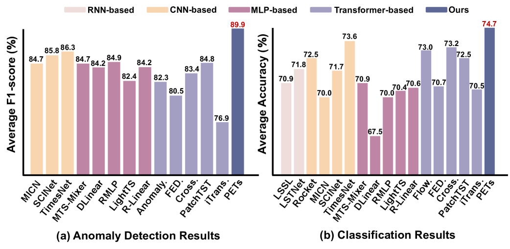
Figure 4: Results of classification and anomaly detection. The results are averaged from several datasets. Higher accuracy and F1 score indicate better performance. The detailed results are presented in Table 17 and  18.

3.6 Anomaly Detection and Classification

Setups. Anomaly detection and classification are fundamental tasks that evaluate the ability to capture subtle mutation information from temporal fluctuations, playing a critical role in applications such as fault diagnosis and predictive maintenance. Due to the differing inductive biases of discriminative and generative tasks, developing a universal model remains a significant challenge, as these tasks require balancing pattern recognition and data distribution modeling. To address this, we conducted extensive experiments on the UEA Time Series Classification Archive [4] and five widely-used anomaly detection benchmarks [64], ensuring a comprehensive evaluation across diverse scenarios.

Results. On the benchmarks of classification and anomaly detection, Pets has achieved consistent state-of-the-art performance in Figure 4, with the accuracy rate and F1-score reaching 74.7% and 89.9% respectively. Notably, compared with popular transformer models such as PatchTST and iTransformer, Pets has witnessed respective enhancements of 5.9% and 16.9% in terms of accuracy and f1-score. It should be noted that the attention architecture augmented by fluctuation pattern has, for the first time, simultaneously attained optimal performance in both generative and discriminative tasks, underlining the fact that Pets can capture universal patterns from diverse scenarios.

3.7 Model Analysis

Table 5: We conducted 4 sets of ablation experiments on all 5 benchmarks. The results evaluate the effectiveness of components.

	Weather	Solar	Electricity	Traffic	ETTh2	Average	Promotion
Pets	0.219	0.187	0.173	0.403	0.360	0.268	-
w/o FPA	0.249	0.242	0.196	0.448	0.398	0.307	14.6%
w/o PPA	0.229	0.199	0.183	0.427	0.383	0.284	5.97%
w/o MPR	0.238	0.202	0.189	0.437	0.392	0.291	8.58%
w/o MPM	0.232	0.197	0.181	0.423	0.376	0.282	5.22%
w/o MoP	0.235	0.208	0.184	0.433	0.383	0.289	7.84%

Ablation Study. To elucidate which components Pets benefits from, we conducted a comprehensive ablation study on the model architecture. As presented in Table 5, we found that removing (w/o) the FPA led to a notable decline in performance. These results may be attributed to the fact that the proposed fluctuation pattern assisted (FPA) module utilizes the captured fluctuation patterns as conditional context, guiding the backbone blocks to focus on modeling specific fluctuation patterns. Specifically, in the challenging multivariate benchmarks such as Solar, Electricity, and Traffic, the proposed fluctuation pattern assisted approach enhanced performance by 29.4%, 13.3%, and 11.2% respectively. Similar results were obtained on other datasets, demonstrating the superiority of this design. In addition, we have also conducted comprehensive ablations on each basic component.

Applicability Study of the Augmentation Strategy. Notably, the proposed Spectrum Decomposition and Amplitude Quantization (SDAQ) and Fluctuation Pattern Assisted (FPA) strategy can be seamlessly integrated into various deep models, in a plug-and-play fashion. This prompts us to investigate its generality by inserting FPA into diverse types of structures. We selected representative baselines composed of divergent underlying architectures. The results in Table 6 validate that the augmentation strategy can significantly elevate model predictive capability. Concretely, the attention-based PatchTST witnessed performance improvements of 34.8% and 17.6% on Solar and ECL respectively. The Linear-based TimeMixer and DLinear achieved enhancements of 14.5% and 19.4% on Traffic. The CNN-based TimesNet showed an improvement of 8.8% on ETTm2. These findings authenticate that the proposed augmentation strategy is applicable to variegated deep architectures.

Table 6: Evaluate the generality of the Pets , Original. as original baseline, +Pets. as pattern-enhanced version by proposed SDAQ and FPA architecture, and Improve. demonstrates the improvement. The detailed results are presented in Table 19.

Datasets		Weather		Solar		Electricity		Traffic		ETTm2		ETTh1
Metrics		MSE	MAE	MSE	MAE	MSE	MAE	MSE	MAE	MSE	MAE	MSE	MAE
PatchTST [2023]	Original.	0.265	0.285	0.287	0.333	0.216	0.318	0.529	0.341	0.290	0.334	0.516	0.484
	+Pets.	0.219	0.255	0.187	0.244	0.178	0.269	0.478	0.299	0.255	0.310	0.415	0.426
	Improve.	17.4%	10.5%	34.8%	26.7%	17.6%	15.4%	9.6%	12.3%	12.1%	7.2%	19.6%	12.0%
TimeMixer [2024b]	Original.	0.240	0.271	0.216	0.280	0.182	0.272	0.484	0.297	0.275	0.323	0.447	0.440
	+Pets.	0.224	0.264	0.188	0.251	0.161	0.254	0.414	0.278	0.263	0.319	0.411	0.421
	Improve.	6.7%	2.6%	13.0%	10.4%	11.5%	6.6%	14.5%	6.4%	4.4%	1.3%	8.1%	4.3%
DLinear [2023]	Original.	0.265	0.315	0.330	0.401	0.225	0.319	0.625	0.383	0.354	0.402	0.461	0.457
	+Pets.	0.245	0.277	0.259	0.276	0.189	0.283	0.504	0.323	0.255	0.313	0.409	0.422
	Improve.	8.3%	12.1%	32.9%	31.2%	16.0%	11.3%	19.4%	15.7%	36.0%	22.1%	11.6%	7.7%
TimesNet [2023]	Original.	0.251	0.294	0.403	0.374	0.193	0.304	0.620	0.336	0.291	0.333	0.495	0.450
	+Pets.	0.241	0.280	0.374	0.340	0.172	0.270	0.578	0.314	0.265	0.297	0.459	0.420
	Improve.	4.0%	4.7%	7.3%	9.1%	10.7%	11.1%	6.7%	6.6%	8.8%	10.8%	7.2%	6.7%

Representation Analysis. As depicted in Fig. 5, we present the initial observed sequence and three decoupled fluctuation sequences. For each, we calculate point-wise attention scores. Visualization validates Pets ’s effectiveness in segregating fluctuation sequences of disparate periods and frequencies. Note that the attention scores on the original sequence show a multi-tiered chaotic structure. In contrast, those of decoupled sequences display distinct periodicity, with line density in score maps effectively reflecting frequency information. Thanks to the hierarchical attention mechanism, Pets can capture both long- and short- wave patterns, while exemplifying robust interpretability.

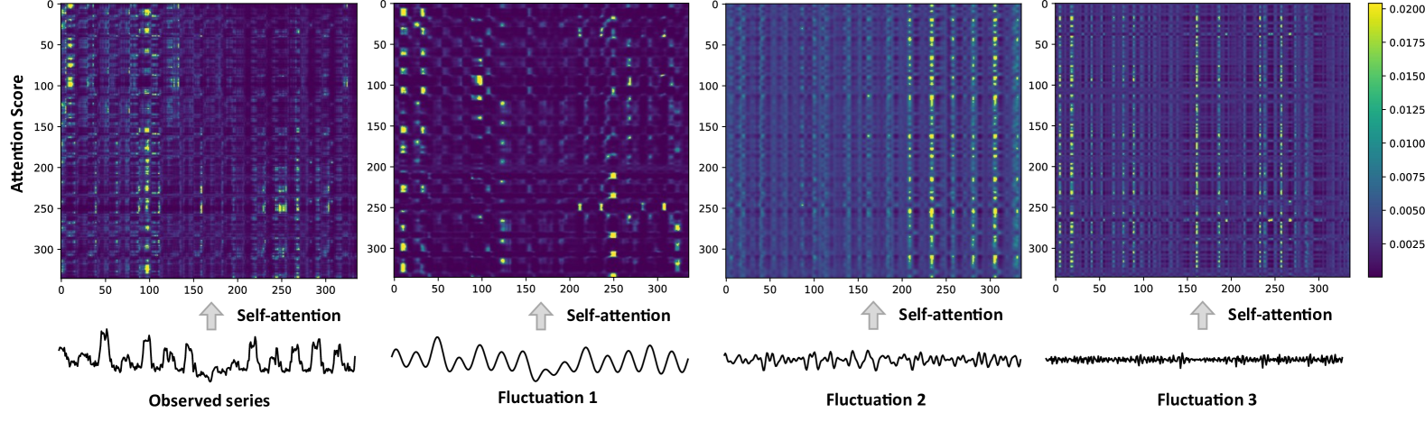
Figure 5: Analysis of the dependency relationships within each single fluctuation pattern. Detailed analysis is in the appendix F.2.

4 Conclusion

We formulate a universal Fluctuation Pattern-Assisted Temporal Architecture (Pets), which comprehensively actuates the modeling and generalization potential of extant methodologies across disparate data domains and task scenarios. Pets discerns the intrinsic augmented ensemble of hybrid fluctuation patterns within time series by adaptively disentangling the dynamically superimposed configurations of multi-periodic fluctuation patterns. Concurrently, To render the augmentation strategy amenable to diverse tasks, PPA and MoP adaptively aggregate the hybrid fluctuation patterns based on energy ranking, enabling the fluctuation patterns highly relevant to the task to dominate the model’s output. Pets has attained state-of-the-art performance in all 8 prevalent time series analysis tasks across 60 benchmarks.

Appendix A Related Work

A.1 Time Series Prediction Models

Prior to the advent of deep learning, the ARIMA model [Zhang, 2003], founded on mathematical theory, was extensively employed in time series prediction tasks. Nevertheless, in the face of time series data possessing nonlinear trends or seasonality, ARIMA encounters difficulties in precisely apprehending the intrinsic characteristics [Kontopoulou et al., 2023]. During the nascent stage of deep learning’s development, models based on Recurrent Neural Networks (RNN) [Shi et al., 2015, Aseeri, 2023] were devised to capture the dependency patterns among time points within time series data. Subsequently, the Temporal Convolutional Network (TCN) [Wu et al., 2023, Luo and Wang, 2024] attracted extensive attention by virtue of its remarkable local modeling capabilities. Nonetheless, the Markovian-based RNN models are inherently flawed in their inability to efficaciously model long-term dependencies [Zhou et al., 2021, Wu et al., 2021]. Meanwhile, the one-dimensional TCN models, circumscribed by the limitations of their receptive fields, fail to capture global dependency [Tang et al., 2020].

During this phase, a profusion of research endeavors burgeoned, with the aim of augmenting the receptive fields of convolutional architectures. MICN [Wang et al., 2023] conducts modeling from a local-global perspective, initially distilling the local traits of the observed sequence and subsequently derives the correlations among all local features to constitute the global characteristics. Meanwhile, TimesNet [Wu et al., 2023] exploits the periodic pattern information to convert the original series into a two-dimensional temporal image and employs two-dimensional convolution to simultaneously model the time series patterns across multiple periods, serving as a supplementation to the global perspective. Moreover, the Multilayer Perceptron (MLP) [Zeng et al., 2023, Xu et al., 2024] founded on pointwise projection has also evinced substantial potential in the time series prediction tasks. Subsequently, Approaches [Zhou et al., 2021, Wu et al., 2021, Zhou et al., 2022a, Liu et al., 2021b] based on the attention mechanism, which directly learned long-term dependency relations and extract global information, have been extensively utilized in long-term prediction tasks. The remarkable methodologies PatchTST [Nie et al., 2023] and iTransformer [Liu et al., 2024] respectively introduced the embedding strategies of "Patch as Token" and "Series as Token" to ameliorate the traditional "Point as Token", and have presently emerged as paradigmatic works in the application of the attention mechanism within the time series.

Certain recent investigations [Wang et al., 2024b, a, Lin et al., 2024], have discerned the inherent challenges of time series data, namely, the superposition and coupling of multiple fluctuation patterns, which present a formidable challenge for time series.

A.2 Frequency Assisted Analysis

Frequency domain enhancement strategies have been astutely implemented in diverse foundational architectures and have attracted extensive attention in the purview of time series analysis. Specifically, FEDformer [Zhou et al., 2022a] has proposed a mixture of expert’s decomposition module and a frequency enhancement mechanism to ameliorate the computational complexity of the attention mechanism. FreTS [Yi et al., 2023] advocates the utilization of MLP to capture the complete perspective and global dependency of the observed sequence within the frequency domain. FITS [Xu et al., 2024] has developed low-pass filters and linear transformations in the complex frequency domain to directly model the mapping relationships between various frequency components of the observed sequence and the predicted sequence in the frequency domain. FilterNet [Yi et al., 2024] introduces learnable frequency filters to extract pivotal temporal patterns, thereby facilitating the efficient handling of high-frequency noise and the utilization of the entire frequency spectrum for prediction. FCVAE [Wang et al., 2024d] introduces frequency domain information as guiding information and utilizes both global and local frequency domain representations to capture heterogeneous periodic patterns and detailed trend patterns, aiming to enhance the accuracy of anomaly detection algorithms. ROSE [Wang et al., 2024c] separates the coupled semantic information in time series data through multiple frequency domain masks and reconstructions, subsequently extracting unified representations across diverse domains.

As expounded above, given that decoupling the mixed fluctuation patterns directly within the temporal domain poses challenges. At the same time, spectrum analysis, by virtue of its inherent advantages of possessing a global perspective and energy compression, has been extensively deployed in prevalent methodologies to fortify the model’s capacity to identify and generalize intricate fluctuation patterns from observed sequences. It is natural to put forward a conjecture:

A.3 Multi-scale and Multi-period Decomposition

Beyond the research route focusing on modeling architectures, the enhancement strategies based on trend-season and multi-scale decomposition have also demonstrated remarkable potential.

In the context of multi-scale decomposition algorithms, Pyraformer [Liu et al., 2021b] incorporates a pyramid attention module, within which the scale architecture simultaneously aggregates features at disparate resolutions and time correlations across diverse scopes. Subsequently, SCINet [Liu et al., 2021a] designs a binary tree structure to extract time series dependencies at various scales from the observed sequence and employs additional channels to compensate for the long-term dependency information deficient in TCN. The recent TimeMixer [Wang et al., 2024b] proposes a multi-scale mixed architecture to disentangle the complex time series patterns in time series prediction and utilizes multi-scale complementarity to enhance the prediction capabilities.

With regard to multi-period decomposition, recent models incorporating multi-periodic designs, such as MSGNet [Cai et al., 2024], which employs frequency domain analysis and adaptive graph convolution to model the correlations among disparate sequences across multiple time scales, thereby capturing prominent periodic patterns. Moreover, MTST [Zhang et al., 2023] concurrently models variegated time patterns at diverse resolutions and utilizes patches of multiple scales to identify different periodic patterns.

Conventional periodic decomposition and multi-scale augmentation algorithms fall short of effectively disentangling disparate fluctuation patterns, as the high-frequency pattern exists only in the seasonal and fine-grained segments and remains superposed and intertwined with other patterns. These approaches mainly focus on prediction and lack the capacity to capture universal temporal patterns applicable to diverse tasks.

Moreover, time series originating from disparate domains typically exhibit markedly heterogeneous compound periodic patterns, which precludes the commonplace multi-period decomposition from accurately partitioning the various periodic patterns. For instance, traffic data is constituted by the superposition of periodic fluctuations at the daily, monthly, and yearly scales, whereas medical physiological signals are more concerned with fine-grained periodic patterns such as those at the second, minute, and hour scales. Even in the presence of ample prior information, the endeavor to model diverse periodic-fluctuation patterns via shared channels remains arduous [Lin et al., 2024].

A.4 Enhancement Strategy

Enhancement strategies represent a potent modality for eliciting the complete potential of deep learning within complex datasets and have witnessed extensive application across vision and natural language. VitComer [Xia et al., 2024] has devised a feature enhancement architecture that is plain, devoid of pre-training, and encompasses a bidirectional fusion and interaction module of CNN-Transformer. This architecture facilitates multi-scale amalgamation of cross-level features, thereby mitigating the problem of restricted local information interchange. VitAdapter [Chen et al., 2022] introduces inductive biases via a supplementary augmentation architecture to compensate for the prior information regarding images that ViT lacks. This paper further investigates the enhancement of fluctuation patterns that are applicable across diverse tasks within time series.

Distinct from prior designs, Pets adaptively converts time series data into fluctuation patterns possessing a fixed energy distribution through amplitude margin filtering and performs adaptive aggregation of the mixed fluctuation patterns in accordance with the energy ranking order, guaranteeing that the fluctuation patterns with high task relevance can dominate the output results of the model.

Appendix B Implementation Details

Datasets Details.

We evaluate the performance of different models for long-term forecasting on 8 well-established datasets, including Weather, Traffic, Electricity, Exchange, Solar-Energy, and ETT datasets (ETTh1, ETTh2, ETTm1, ETTm2). Furthermore, we adopt PeMS and M4 datasets for short-term forecasting. We detail the descriptions of the dataset in Table 7.To comprehensively evaluate the model’s performance in time series analysis tasks, we further introduced datasets for classification and anomaly detection. The classification task is designed to test the model’s ability to capture coarse-grained patterns in time series data, while anomaly detection focuses on the recognition of fine-grained patterns. Specifically, we used 10 multivariate datasets from the UEA Time Series Classification Archive (2018) for the evaluation of classification tasks. For anomaly detection, we selected datasets such as SMD (2019), SWaT (2016), PSM (2021), MSL, and SMAP (2018). We detail the descriptions of the datasets for classification and anomaly detection in Table 8 and Table 9

Table 7: Dataset detailed descriptions. The dataset size is organized in (Train, Validation, Test).

Tasks	Dataset	Dim	Series Length	Dataset Size	Frequency	Forecastability$\ast$	Information
	ETTm1	7	{96, 192, 336, 720}	(34465, 11521, 11521)	15min	0.46	Temperature
	ETTm2	7	{96, 192, 336, 720}	(34465, 11521, 11521)	15min	0.55	Temperature
	ETTh1	7	{96, 192, 336, 720}	(8545, 2881, 2881)	15 min	0.38	Temperature
	ETTh2	7	{96, 192, 336, 720}	(8545, 2881, 2881)	15 min	0.45	Temperature
Long-term	Electricity	321	{96, 192, 336, 720}	(18317, 2633, 5261)	Hourly	0.77	Electricity
Forecasting	Traffic	862	{96, 192, 336, 720}	(12185, 1757, 3509)	Hourly	0.68	Transportation
	Exchange	8	{96, 192, 336, 720}	(5120, 665, 1422)	Daily	0.41	Weather
	Weather	21	{96, 192, 336, 720}	(36792, 5271, 10540)	10 min	0.75	Weather
	Solar-Energy	137	{96, 192, 336, 720}	(36601, 5161, 10417)	10min	0.33	Electricity
	PEMS03	358	12	(15617,5135,5135)	5min	0.65	Transportation
	PEMS04	307	12	(10172,3375,3375)	5min	0.45	Transportation
	PEMS07	883	12	(16911,5622,5622)	5min	0.58	Transportation
Short-term	PEMS08	170	12	(10690,3548,265)	5min	0.52	Transportation
Forecasting	M4-Yearly	1	6	(23000, 0, 23000)	Yearly	0.43	Demographic
	M4-Quarterly	1	8	(24000, 0, 24000)	Quarterly	0.47	Finance
	M4-Monthly	1	18	(48000, 0, 48000)	Monthly	0.44	Industry
	M4-Weakly	1	13	(359, 0, 359)	Weakly	0.43	Macro
	M4-Daily	1	14	(4227, 0, 4227)	Daily	0.44	Micro
	M4-Hourly	1	48	(414, 0, 414)	Hourly	0.46	Other

• $\ast$ The forecastability is calculated by one minus the entropy of Fourier decomposition of time series [Goerg, 2013]. A larger value indicates better predictability.

Table 8: Datasets and mapping details of UEA dataset [Bagnall et al., 2018].

Dataset	Sample Numbers(train set,test set)	Variable Number	Series Length
EthanolConcentration	(261, 263)	3	1751
FaceDetection	(5890, 3524)	144	62
Handwriting	(150, 850)	3	152
Heartbeat	(204, 205)	61	405
JapaneseVowels	(270, 370)	12	29
PEMSSF	(267, 173)	963	144
SelfRegulationSCP1	(268, 293)	6	896
SelfRegulationSCP2	(200, 180)	7	1152
SpokenArabicDigits	(6599, 2199)	13	93
UWaveGestureLibrary	(120, 320)	3	315

Table 9: Datasets and mapping details of anomaly detection dataset.

Dataset	Dataset sizes(train set,val set, test set)	Variable Number	Sliding Window Length
SMD	(566724, 141681, 708420)	38	100
MSL	(44653, 11664, 73729)	55	100
SMAP	(108146, 27037, 427617)	25	100
SWaT	(396000, 99000, 449919)	51	100
PSM	(105984, 26497, 87841)	25	100

Baseline Details.

To assess the effectiveness of our method across various tasks, we select 27 advanced baseline models spanning a wide range of architectures. Specifically, we utilize CNN-based models: MICN [2023], SCINet [2021a], and TimesNet [2023]; MLP-based models: TimeMixer [2024b], LightTS [2023], and DLinear [2023]; RMLP&RLinear [2023a] and Transformer-based models: iTransformer [2024], PatchTST [2023], Crossformer [2021], FEDformer [2022a], Stationary [2022], Autoformer [2021], and Informer [2021]. These models have demonstrated superior capabilities in temporal modeling and provide a robust framework for comparative analysis. For specific tasks, TiDE [2023], FiLM [2022b], N-HiTS [2022], and N-BEATS [2019] address long- or short-term forecasting; Anomaly Transformer [2021] and MTS-Mixers [2023b] target anomaly detection; while Rocket [2023a], LSTNet [2017], LSSL [2021], and Flowformer [2022] are utilized for classification. Few/zero-shot forecasting tasks employ ETSformer [2022], Reformer [2020], and LLMTime [2024].

Metric Details.

Regarding metrics, we utilize the mean square error (MSE) and mean absolute error (MAE) for long-term forecasting. In the case of short-term forecasting, we follow the metrics of SCINet [Liu et al., 2021a] on the PeMS datasets, including mean absolute error (MAE), mean absolute percentage error (MAPE), root mean squared error (RMSE). As for the M4 datasets, we follow the methodology of N-BEATS [Oreshkin et al., 2019] and implement the symmetric mean absolute percentage error (SMAPE), mean absolute scaled error (MASE), and overall weighted average (OWA) as metrics. It is worth noting that OWA is a specific metric utilized in the M4 competition. The calculations of these metrics are:

RMSE $$=(\sum_{i=1}^{F}(\mathbf{X}_{i}-\widehat{\mathbf{X}}_{i})^{2})^{\frac{1}{2}},\text{MAE}=\sum_{i=1}^{F}|\mathbf{X}_{i}-\widehat{\mathbf{X}}_{i}|,$$

SMAPE $$=\frac{200}{F}\sum_{i=1}^{F}\frac{|\mathbf{X}_{i}-\widehat{\mathbf{X}}_{i}|}{|\mathbf{X}_{i}|+|\widehat{\mathbf{X}}_{i}|},\text{MAPE}=\frac{100}{F}\sum_{i=1}^{F}\frac{|\mathbf{X}_{i}-\widehat{\mathbf{X}}_{i}|}{|\mathbf{X}_{i}|},$$

MASE $$=\frac{1}{F}\sum_{i=1}^{F}\frac{|\mathbf{X}_{i}-\widehat{\mathbf{X}}_{i}|}{\frac{1}{F-s}\sum_{j=s+1}^{F}|\mathbf{X}_{j}-\mathbf{X}_{j-s}|},$$

OWA $$=\frac{1}{2}\left[\frac{\text{SMAPE}}{\text{SMAPE}_{\textrm{Na\"{\i}ve2}}}+\frac{\text{MASE}}{\text{MASE}_{\textrm{Na\"{\i}ve2}}}\right],$$

where $s$ is the periodicity of the data. $\mathbf{X},\widehat{\mathbf{X}}\in\mathbb{R}^{F\times C}$ are the ground truth and prediction results of the future with $F$ time pints and $C$ dimensions. $\mathbf{X}_{i}$ means the $i$-th future time point.

Experiment Details.

To valudate the reproducibility of all experimental results, each experiment was executed three times and the average results were presented. The code was implemented on the basis of PyTorch [Paszke et al., 2019] and executed on multiple NVIDIA V100 40GB GPUs. The initial learning rate was configured as either $10^{-3}$ or $10^{-4}$, and the model was optimized by means of the ADAM optimizer [Kingma and Ba, 2014] with L2 loss. The batch size was designated as 128. By default, Pets encompasses all 4 layers, with each layer incorporating PPA (adapter block), MPR, MPM, and backbone block. Moreover, each dataset inherently supports 3 fluctuation patterns and an additional trend component. To ensure the impartiality and efficacy of the experimental results, we replicated all the experimental configurations of TimeMixer [Wang et al., 2024b] and employed the experimental results of certain baselines presented in its original publication.

Appendix C Further Discussion for Pets

C.1 Advantages of Pets over multi-resolution-based models for diverse tasks

In the existing multi-resolution approaches, TimeMixer generates multi-scale sequences via downsampling only in the time domain and establishes connections between different-scale representations using linear layers. N-BEATS and N-HITS imposes constraints on expansion coefficients as prior information to guide layers to learn specific time-series features (e.g., seasonality), enabling interpretable sequence decomposition. However, these methods inherently rely on traditional seasonal-trend decomposition and multi-scale decomposition, which fail to achieve complete decoupling—for example, composite high-frequency components remain coupled in seasonal or fine-grained parts.

In contrast, our proposed method introduces a novel frequency-domain-based decoupling algorithm (SDAQ), which transforms input sequences into the frequency domain and decouples patterns explicitly in the frequency domain, allowing for more precise reconstruction of multi-period fluctuations. This ensures lossless and independent decomposition, resolving the coupling of high-frequency components often present in traditional time-domain approaches.

Concretely, SDAQ transforms input sequences into the frequency domain and explicitly separates them into three frequency components (bands), ensuring lossless and non-overlapping distribution of information from observed sequences into three decoupled sequences. Then SDAQ inverse-transforms each group back to the time domain, thus resolving the information coupling between different frequency bands.

C.2 The Distinction between zero-shot transfer and zeros-shot forecasting

In Section 3.5, we presented the detailed results of the proposed approach under the zero-shot scenario. However, unlike existing time series foundation models that directly conduct inference on the target data domain after pre-training. In our designed experiments, Pets and some recent small-scale models (including PatchTST [Nie et al., 2023], TimesNet [Wu et al., 2023], and TimeMixer [Wang et al., 2024b]) are first trained from scratch in source data domain and then predict in the unseen target data domain.

To avoid ambiguity, we refer to these two forecasting paradigms as Zero-shot Forecasting and Zero-shot Transfer. In the past, zero-shot and few-shot tasks were only regarded as benchmarks for evaluating large-scale models (such as large language models and time series foundation models). However, some recent works [Zhou et al., 2023, Jin et al., 2023, Gruver et al., 2024, Wang et al., 2024a] commonly choose zero-shot and few-shot forecasting as one of the tasks for evaluating model performance. These approaches believe that cross-domain generalization and robustness are significant capabilities of purpose general model, which are crucial for addressing out-of-distribution (OOD) issues and establishing more powerful general time series models.

C.3 The selection of the mother wavelet in the continuous wavelet transform (CWT)

In the open source code, we choose the Haar function as the mother wavelet function. As a compactly supported orthogonal wavelet function, Haar wavelets only consider local regions during decomposition, leading to high computational efficiency that helps reduce Pets’ overall complexity. Additionally, Haar wavelets excel in decomposing high-frequency components, enhancing Pets ’ generalization capability for handling diverse fluctuation patterns across frequencies. In Pets , we selected Haar wavelets due to their extensive application in time-series analysis. Further exploring the potential advantages of other wavelet functions for decoupling composite fluctuation patterns will be part of our future work.

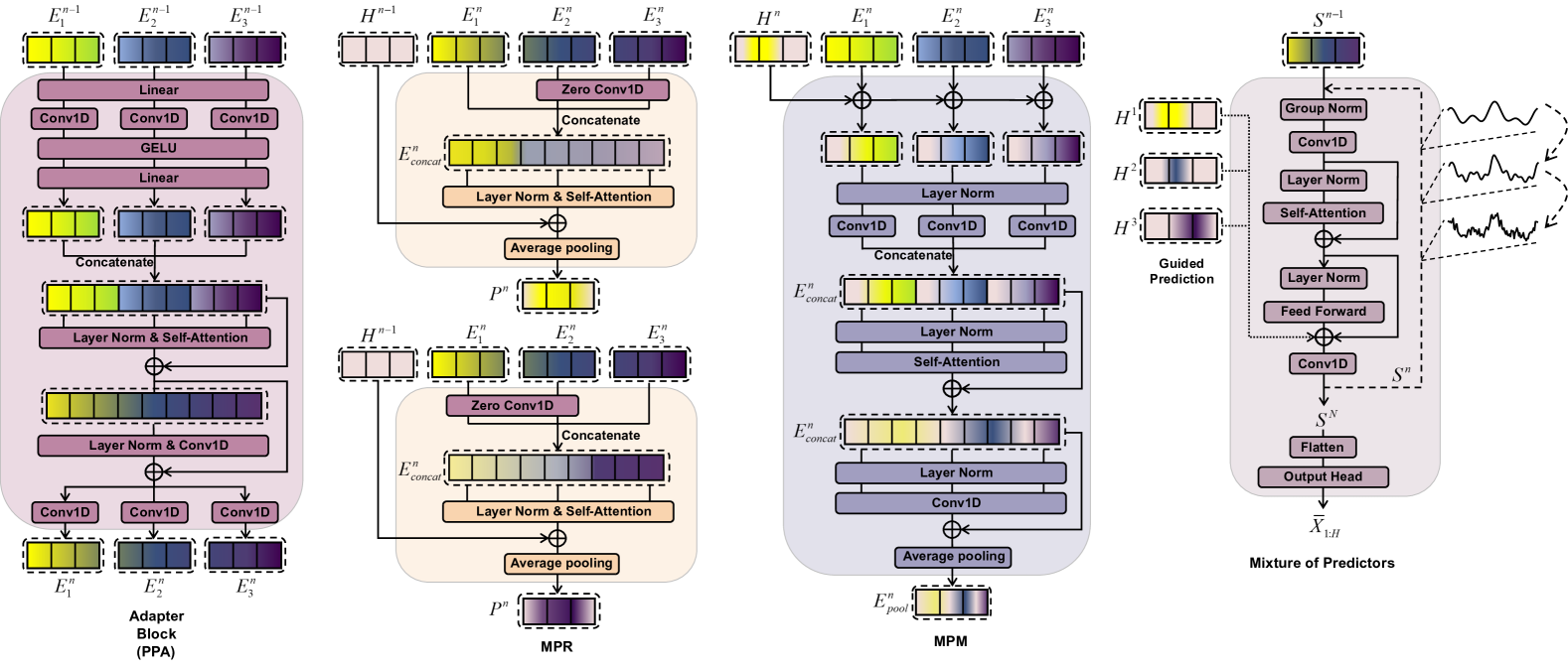
Figure 6: The detailed structure of the proposed model encompasses components Periodic Prompt Adapter (PPA), Multi-fluctuation Patterns Rendering (MPR), Multi-fluctuation Patterns Mixing (MPM) and mixture of predictors (MoP).

Appendix D Details of Model design

D.1 Fluctuation Pattern Assisted

In this section, we present the detailed architecture of the proposed Pets , encompassing Periodic Prompt Adapter (PPA), Multi-fluctuation Patterns Rendering (MPR), Multi-fluctuation Patterns Mixing (MPM) and mixture of predictors (MoP), as shown in Fig. 6. Specifically, within the adapter block, the input tokens of diverse fluctuation patterns are passed through successive linear, conv1d, and activation layers, after which they are concatenated to obtain tokens of a comprehensive pattern. These tokens then pass through a self-attention mechanism and a feed-forward structure connected by a residual connection, yielding a deep representation. Finally, this deep representation is processed by three independent conv1d layers to generate a single fluctuation pattern for the subsequent stage.

In the MPR, we devised a novel variable zero-convolution gate. This gate is designed to make MPR at different stages inclined to learn information from designated pattern tokens. For instance, in the MPR of the first layer, the zero-convolution layer is inserted into the short-wave and high-frequency pattern channels. This makes the current MPR tend to learn temporal representations from long-wave patterns. Meanwhile, all the weights of the zero-convolution layer are fixed at zero only during initialization and are permitted to participate in subsequent training. This ensures that the convolution gate has a distinct bias in the initial training phase, while in subsequent training, each layer of MPR can flexibly capture comprehensive temporal representations from all pattern tokens.

The MPM simultaneously receives two inputs: the hidden representation and a set of fluctuation patterns. The hidden representation contains the information of fluctuation patterns already learned by the model, which serves as conditional information to guide the model in capturing more profound fluctuation patterns. Additionally, we present a novel hybrid predictor capable of gradually generating the fluctuation details of future sequences.

D.2 Fluctuation Pattern Assisted

In real world scenarios of time series analysis, the vast majority of datasets consist of multiple time series, and there are evident dependencies among these channels. For instance, modern industrial equipment often incorporates multiple groups of sensors. Each group of sensors focuses on collecting signals from different parts. Meanwhile, for sensitive segments, sensors for different physical signals may be configured, such as photosensitive, current, and temperature sensors. Additionally, in medical diagnosis scenario, the condition of patient is jointly determined by multiple physiological signals, such as heart rate, blood pressure, and the surface temperature at the lesion site.

These complex and variable realm scenarios demand that a model must capture comprehensive temporal fluctuation information from all channels to make accurate predictions and judgments about samples. To address these challenges, supporting multi-channel data input has naturally become a latent requirement for general models. In this section, we elaborate on how the model models the inter-channel dependencies.

As depicted in Fig. 7, time series from different channels undergo independent decoupling and patch-based embedding operations, resulting in an identical set of long- and short-wave pattern tokens. These tokens are re-concatenated into two groups of representations according to the principles of the same fluctuation pattern and the same channel. Subsequently, we first calculate the attention scores among the fluctuation patterns and then among the channels.

This flexible computational strategy for the attention mechanism ensures that, for each token, both other fluctuation patterns from the same channel and the same fluctuation pattern from different channels are visible. Additionally, the spectrum-quantization decoupling operation guarantees that, compared with the coupled and superimposed observation sequences, each decoupled fluctuation pattern exhibits more distinct periodic characteristics. Meanwhile, the same fluctuation patterns from different channels also demonstrate explicit convergence, which significantly alleviates the potential heterogeneity among different channels. These advantages ensure that the proposed Pets can gain an edge on datasets with a large number of channels, as exemplified by the experimental results of PEMS presented in Table. 16.

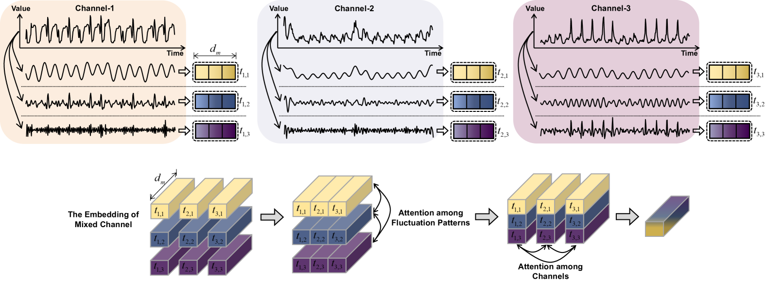
Figure 7: We present the design details of the proposed Pets under the channel-mixing design. It incorporates two key configurations, the attention mechanism among fluctuation patterns and the attention mechanism among channels.

D.3 Model Hyperparameter Sensitivity Analysis

In the design of SDAQ, the energy in time series is mainly concentrated in the low-frequency bands, and the energy of the bands continuously decays as the frequency increases. This implies that by dividing only a limited number of frequency bands, the input series can be decoupled into multiple fluctuation patterns without overlapping. Additionally, when the number of divided frequency bands is excessive, limited information falling within the high-frequency range will be further split. This leads to the decoupled series containing a large amount of noise and a small amount of information, thereby reducing the predictive performance of the model. Based on these considerations, we fix the number of decoupled fluctuation patterns as $K\textit{=}3$, and set the energy ratio as $(\mu_{1},\mu_{2})$.

In the design of component FPA and MoP, the model consists of $N$ consecutive composite layers. Each layer contains single adapter block (PPA), single backbone block, single MPM, and single MPR. Correspondingly, the hybrid predictor is also composed of $N$ predictors with the same structure. Additionally, both the original sequence and the decoupled sequence yield $P_{L}$ tokens after the patch-based embedding operation, where the dimension of each token is $P_{d}$.

In order to verify the sensitivity of Pets to hyperparameter selection, the Table 10 shows the performance of Pets with different parameter scales on multiple benchmarks. Where the model parameter combinations include $(N,P_{d})\textit{=}(3,16),(4,32),(6,128)$ and $(\mu_{1},\mu_{2})\textit{=}(0.3,0.6),(0.4,0.8),(0.7,0.9)$, with a fixed forecasting window of $96$, and a performance metric of MSE. By default, the hyperparameters of Pets are fixed to $N\textit{=}4$, $P_{d}\textit{=}32$ and $(\mu_{1},\mu_{2})\textit{=}(0.7,0.9)$, all experimental results presented follow this setting.

Table 10: To verify the sensitivity of Pets to hyperparameter selection, we show the performance of Pets with different parameter scales on multiple benchmarks, with a fixed forecasting window of 96, and a performance metric of MSE.

Hyperparameter		ETTh1	ETTh2	ETTm1	ETTm2	Weather	ECL	Traffic
$\mu_{1},\mu_{2}$=0.3,0.6	L=3,D=16	0.398	0.327	0.304	0.170	0.155	0.139	0.394
	L=4,D=32	0.389	0.322	0.289	0.177	0.152	0.144	0.412
	L=6,D=128	0.395	0.331	0.295	0.173	0.159	0.148	0.415
$\mu_{1},\mu_{2}$=0.4,0.8	L=3,D=16	0.371	0.292	0.291	0.167	0.146	0.140	0.375
	L=4,D=32	0.378	0.304	0.279	0.163	0.145	0.135	0.381
	L=6,D=128	0.383	0.315	0.292	0.170	0.152	0.141	0.392
$\mu_{1},\mu_{2}$=0.7,0.9	L=3,D=16	0.364	0.298	0.274	0.164	0.142	0.132	0.378
	L=4,D=32	0.385	0.334	0.289	0.164	0.154	0.145	0.388
	L=6,D=128	0.389	0.331	0.282	0.173	0.159	0.143	0.395

D.4 Comprehensive complexity analysis

In this section, we provide a detailed analysis of the computational complexity of Pets’ three main components (SDAQ, FPA, and MoP) and address the specific concerns regarding wavelet transform, spectral quantization, and multi-stage predictors. Pets consists of three main components: SDAQ, FPA, and MoP.

The computational complexity of SDAQ involves three steps: (1) transforming an input sequence of length $L$ into a time-frequency spectrogram with $\lambda$ scales using an FFT-optimized Continuous Wavelet Transform (CWT), which reduces convolution operations to $O(\lambda\cdot L\log L)$; (2) partitioning the spectrogram into three subgraphs based on energy distribution, an operation with negligible complexity; and (3) reconstructing each subgraph into the time domain via inverse wavelet transform (iWT), with the same $O(\lambda\cdot L\log L)$ complexity. Together, SDAQ operates with an overall complexity $O(\lambda\cdot L\log L)$.

The FPA and MoP modules consist of $N$ composite layers, each containing lightweight operations such as 1D convolutions, self-attention, and linear layers. After patching, the tensor shape is $Bd\times P_{L}\times P_{d}$, where $P_{L}$ is the number of tokens and $P_{d}$ is the token dimension. Therefore, linear layer and one-dimensional convolution computation complexity is $O\left(\left(P_{L}\right)^{2}+\left(P_{d}\right)^{2}\right)$, and the computational complexity of attention is $O(P_{L}(P_{d})^{2})$. Note that $P_{L}P_{d}=L$, So there is $O\left(\left(P_{L}\right)^{2}+\left(P_{d}\right)^{2}\right)\geq O\left(2P_{L}P_{d}\right)=O\left(L\right)$ and $O\left(P_{L}\left(P_{d}\right)^{2}\right)=O\left(LP_{d}\right)$. These modules have an overall complexity of $O(L+LP_{d})$, ensuring efficient processing while capturing complex patterns. Regarding the specific processes mentioned:

• Wavelet Transform: Used in SDAQ, the wavelet transform (CWT and iWT) operates with a combined complexity of $O(\lambda\cdot L\log L)$, introducing computational overhead but maintaining scalability through FFT optimization.

• Spectral Quantization: This step partitions the spectrogram into three subgraphs based on frequency energy distribution. The complexity is negligible as it involves simple calculations and indexing.

• Multi-Stage Predictors: Incorporated in FPA and MoP, these predictors rely on 1D convolutions, self-attention, and linear layers, with complexity $O(L+LP_{d})$. This design ensures a balance between computational cost and the ability to model diverse fluctuation patterns effectively.

Furthermore, to further demonstrate Pets’ real-world inference overhead, we present inference speed (ms/iter) and memory usage (GB) during training on the ETTm1 dataset for a forecast horizon of 720 in the Table 11.

Table 11: Comparison of computational complexity between the proposed Pets and existing methods.

Metric	TiDE	TimeMixer	PatchTST	Pets	iTransformer	SCINet	TimesNet	FEDformer
Training Time (ms/iter)	263	271	319	376	435	454	477	722
Memory Cost (GB)	2.92	3.14	4.95	6.17	7.92	5.91	6.72	8.44

D.5 Algorithm for training of Pets

We provide the training procedure of Pets in Algorithm 1, which are described in Section 2.

Where $p_{\textit{emb}}$ and $\left(\overline{h}_{m},\overline{h}_{c},\overline{h}_{b},\overline{h}_{a}\right)$ together serve as the condition variable $c$, $\tilde{Y}_{1:H}^{t-1}\in\mathbb{R}^{Bd\times P_{H}\times P_{d}}$ and $\hat{Y}_{1:H}^{t-1}\in\mathbb{R}^{Bd\times P_{H}\times P_{d}}$ represent the conditional and unconditional outputs of the denoising network, respectively. Furthermore, $Y_{1:H}^{t-1}$ as the final result, and $\lambda$ is a parameter that controls the proportion of conditional and unconditional generation in the final result ($\lambda\textit{=7.5}$ for our experiment)

Algorithm 1 Training of Pets

1: Input: The observation series $X_{-L+1:0}\in\mathbb{R}^{B\times d\times L}$ and prediction series $X_{1:H}\in\mathbb{R}^{B\times d\times H}$, the hyperparameters: the model depth $N$, the feature dimension $P_{d}$, the spectral width $\lambda$, along with the energy thresholds $(\mu_{1},\mu_{2})$ and the iteration $N_{\mathrm{iter}}$.

2: Output: Optimized Pets consisting of $N\times$ FPAs and MoP.

3: for  $i=1$ to $N_{\mathrm{iter}}$ do

4:  Channel Independent: $X_{-L+1:0}\in\mathbb{R}^{B\times d\times L}\to X_{-L+1:0}\in\mathbb{R}^{Bd\times L}$;Temporal-Spectral Decomposition by $CWT_{\lambda}$: $X_{-L+1:0}\in\mathbb{R}^{Bd\times L}\to A\in\mathbb{R}^{Bd\times L\times\lambda}$; Amplitude Quantization Phase: $A\in\mathbb{R}^{Bd\times L\times\lambda}\to A^{1:K}\in\mathbb{R}^{Bd\times L\times\lambda}\to X_{-L+1:0}^{1:K}\textit{=}iWT(A^{1:K})\in\mathbb{R}^{Bd\times L}$;Patching Instance and Embedding: $X_{-L+1:0}\in\mathbb{R}^{Bd\times L}\to E^{0}\in\mathbb{R}^{Bd\times P_{L}\times P_{d}}$, $\{X_{-L+1:0}^{k}\in\mathbb{R}^{Bd\times L}\}_{k\in[1,K]}\to\{E_{k}^{0}\in\mathbb{R}^{Bd\times P_{L}\times P_{d}}\}_{k\in[1,K]}$;

5:  for  $n=1$ to $N$ do

6:   In the Periodic Prompt Adapter block: $E_{k}^{n-1}\textit{=}Conv1D(Linear(E_{k}^{n-1})^{\top})^{\top},E_{k}^{n-1}\textit{=}Dropout(Linear(Act(E_{k}^{n-1})))$; $E_{concat}^{n-1}\textit{=}Concatenate(\{E_{k}^{n-1}\}_{k\in[1,K]})$; $E_{concat}^{n-1}\textit{+=}SelfAttn(E_{concat}^{n-1}),E_{concat}^{n-1}\textit{+=}Conv1D(E_{concat}^{n-1})$; $E_{k}^{n}\textit{=}Conv1D_{k}(E_{concat}^{n-1})_{k\in[1,K]}$;

7:   In the Multi-fluctuation Patterns Rendering block: $\left\{E_{k}^{n}\right\}_{k\in[1,n-1]\cup[n+1,K]}=ZeroConv1d\left(\left\{E_{k}^{n}\right\}_{k\in[1,n-1]\cup[n+1,K]}\right)$; $E_{concat}^{n}\textit{=}Concatenate(\{E_{k}^{n}\}_{k\in[1,K]})$; $E_{concat}^{n}\textit{+=}SelfAttn(E_{concat}^{n}),E_{concat}^{n}\textit{+=}Conv1D(E_{concat}^{n})$; $P^{n}~\textit{=}~H^{n-1}\textit{+}Pool(E_{concat}^{n}),~where~H^{0}\textit{=}E^{0}$;

8:   In the Backbone block: $H^{n-1}\textit{+=}SelfAttn(H^{n-1}),~where~H^{0}\textit{=}E^{0}$; $H^{n}\textit{=}P^{n}\textit{+}H^{n-1}\textit{+}FFN(H^{n-1})$;

9:   In the Multi-fluctuation Patterns Mixing block: $E_{k}^{n}\textit{=}Conv1D(E_{k}^{n}\textit{+}H^{n})_{k\in[1,K]},E_{concat}^{n}\textit{=}Concatenate(\{E_{k}^{n}\}_{k\in[1,K]})$; $E_{concat}^{n}\textit{+=}SelfAttn(E_{concat}^{n}$; $E_{pool}\textit{=}Pool(E_{concat}^{n}\textit{+}Conv1D(E_{concat}^{n}))),\{E_{k}^{n}\textit{=}E_{k}^{n}\textit{+}E_{pool}^{n}\}_{k\in[1,K]}$;

10:  end for$E_{average}^{N}=\left(\sum_{k=1}^{K}E_{k}^{N}\right)/K$;

11:  for  $n=1$ to $N$ do

12:   In the Mixture of Predictors: $S^{n}\textit{+=}Selfattn(Conv1D(S^{n})),~where~S^{0}\textit{=}E_{average}^{N}$; $S^{n\textit{+}1}\textit{=}Conv1D(S^{n}\textit{+}H^{n}\textit{+}FFN(S^{n}))$;

13:  end for

14:  Obtain the prediction result through projection layer: $\overline{X}_{1:H}~\textit{=}~OutputHead(Flatten(S^{N}))$,

15:  Update model parameters based on $\mathcal{L}_{mse}$ gradient. $\mathcal{L}_{mse}\textit{=MSE}\left(X_{1:H},\overline{X}_{1:H}\right)$.

16: end for

Appendix E Pets ’s limitations

E.1 High arithmetic overhead and time cost.

In Table 11, the computational cost of Pets is higher than that of the popular TimeMixer and PatchTST. Therefore, the computational cost serves as the main limitation of Pets . According to our analysis in Section D.4, the computational cost of Pets mainly stems from its frequency-domain-based composite pattern decoupling algorithm, SDAQ.

Although SDAQ thoroughly addresses the issue of different frequency components being coupled together, computing the spectrogram requires a substantial amount of time. In fact, the complexity of SDAQ is mainly caused by the Continuous Wavelet Transform (CWT) and the Inverse Continuous Wavelet Transform (iCWT). The advantage of introducing CWT is that the spectrogram has both frequency and time domains. This means that it can effectively represent the compositional structure of the frequency components in the original sequence as they change over time, which is crucial for the analysis of non-stationary time series. However, CWT leads to a huge computational complexity.

Considering these trade-offs, we propose replacing CWT with the Fast Fourier Transform (FFT) in SDAQ. The improved Pets can still achieve the lossless and non-overlapping decoupling of the original sequence into subsequences with different fluctuation patterns. At the same time, it can significantly reduce the computational cost of SDAQ, bringing the computational cost of Pets down to the same level as that of the popular TimeMixer.

Appendix F Representation Analysis

F.1 Linear Weights

For intuitive illustration of the mapping relationship between the input sequence and the predicted sequence in the frequency-domain space across different tasks, we first transform the original sequence to the frequency domain via the Fourier transform. Subsequently, we employ the linear layer to map the frequency components of the observed sequence to those of the predicted sequence. Finally, the frequency components of the predicted sequence are transformed back to the time domain through the inverse Fourier transform, thereby obtaining the predicted sequence, as $Y\textit{=}iFT(Linear(FT(X)))$

We conducted comprehensive experiments on benchmarks composed of 4 tasks (forecasting, imputation, anomaly detection, and classification) and a total of 20 datasets. Fig. 8 presents the visualization of the linear weights between the original and generated sequence in the frequency domain, and diverse tasks exhibit distinct active patterns. Specifically, in the tasks of prediction, imputation, and anomaly detection, the weight scores are concentrated around the diagonal positions. Specifically, in prediction, the weights are preponderantly distributed within the low-frequency components (the light blue regions in Fig. 8 (a)). For imputation, the weights clustered on the mapping of the input and output sequences at identical frequency components (the diagonal regions in Fig. 8(b)). This indicates that for generative tasks, the frequency-domain components of the input and output sequences tend to establish a comprehensive mapping relationship. In classification Fig. 8(d), the weights are stochastically dispersed throughout the global scope. Meanwhile, anomaly detection Fig. 8(c) amalgamates the characteristics of sundry tasks. Moreover, conventional decomposition and multi-scale augmentation algorithms fall short of effectively disentangling disparate fluctuation patterns, as the high-frequency pattern exists only in the seasonal and fine-grained segments and remains superposed and intertwined with other patterns.

F.2 Intra-pattern Dependencies

In Fig. 9 and 10, the original time series samples are decoupled into three independent fluctuation modes, and the fluctuation modes 1 to 3 exhibit the pattern characteristics from long-to-short period and low-to-high frequency respectively. We then compute the global dependencies between all time points in each fluctuation pattern, and the top plot shows the attention score visualization for each pattern. Specifically, in the original sequence, the dependencies between time points are chaotic, which is caused by the mutual coupling between multiple periodic patterns in the original sequence. In contrast, the decoupled fluctuation patterns show distinct periodic variation characteristics. Concretely, in the fluctuation pattern 1, the bright yellow blob shows a sparse distribution characteristic, which means that the attention mechanism learns the dependence between long periods from it, which we call the long wave pattern. However, in the fluctuation mode 3, the bright yellow blobs show the characteristics of clustered distribution, and the attention learns the dependence between short periods from it, which we call the short-wave mode.

F.3 Inter-pattern Dependencies

In Fig. 11, Fig. 12, Fig. 13 and Fig. 14, we present the visualization of the importance of different fluctuation patterns for specific downstream tasks. We first decouple the observed sequence into three fluctuating sequences. Subsequently, each of these fluctuating sequences undergoes a patch-based embedding operation to obtain three groups of pattern tokens, where each set contains 40 tokens. Finally, all 120 tokens are concatenated in the order from low-frequency pattern to high-frequency pattern, and then fed into the transformer, where the attention scores between these tokens in different tasks are calculated.

Specifically, in the forecasting and imputation tasks, we notice that the yellow bright spots only appear in the top left corner, which means that there is a strong dependence between the shortwave patterns ($x\in[0,40]$) of the input sequence, short wave (long period) patterns are crucial for both forecasting and imputation tasks. This is also in line with cognition, since long-term trends are important for prediction tasks, and high-frequency oscillations in them are likely due to noise. In contrast, in the anomaly detection and classification tasks, the yellow bright spot distribution will appear in the small right corner and the bottom left corner, which means that the high-frequency perturbation is critical for the classification and anomaly detection tasks. It can be understood that abrupt signals are often caused by reasons such as mechanical failures, and therefore these high-frequency patterns are very important for discriminative tasks.

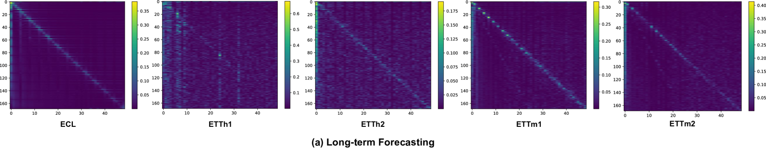
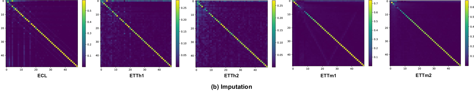
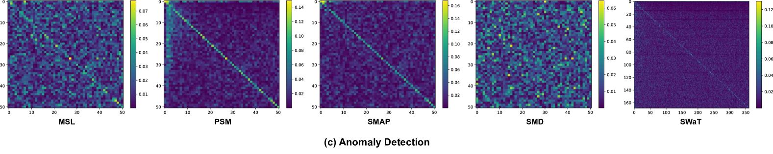
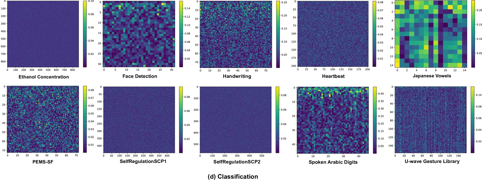
Figure 8: Representation Analysis Based on Visualization of Linear Weights. We utilize the linear layer to enable the establishment of a mapping relationship between the frequency components of the input and output sequences in the frequency - domain space. Each task exhibits a specific mapping pattern.

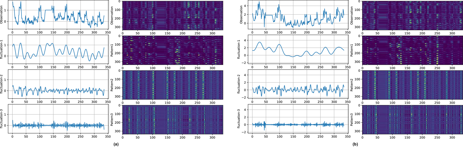
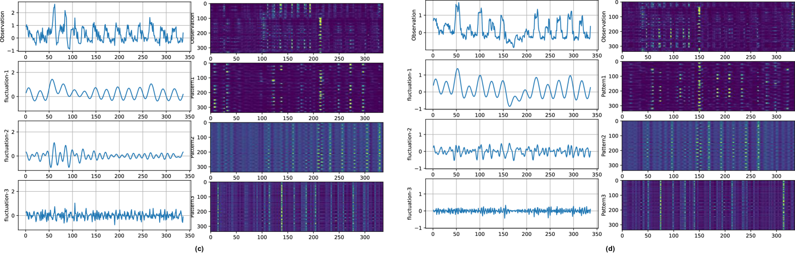
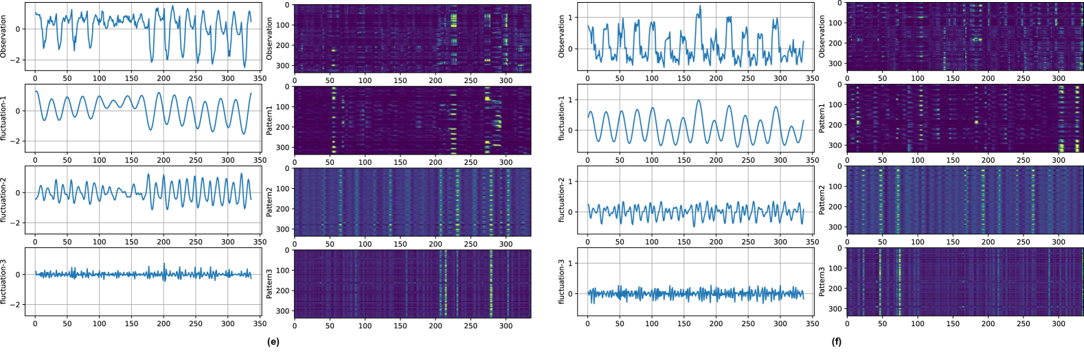
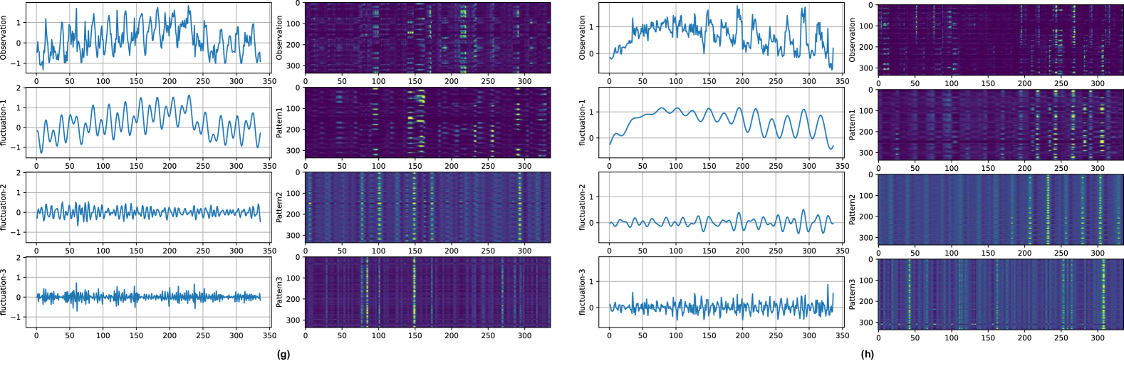
Figure 9: Visualization of the decomposition algorithm on the ETTh1 dataset. Additionally, we present the point-wise attention scores calculated on the observed sequence and the three decomposed sequences.

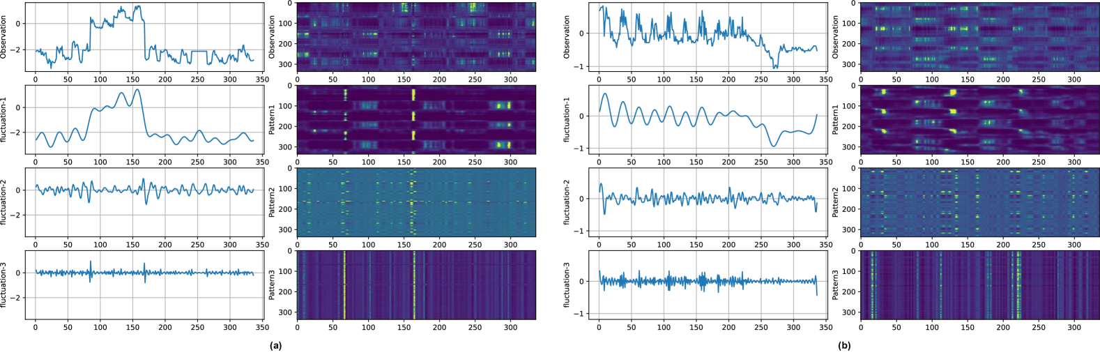
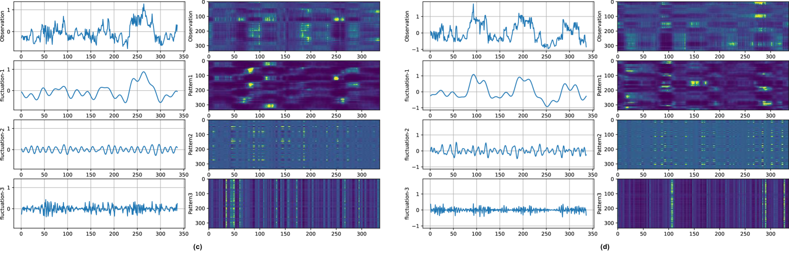
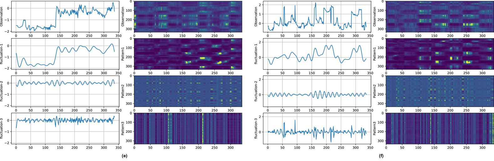
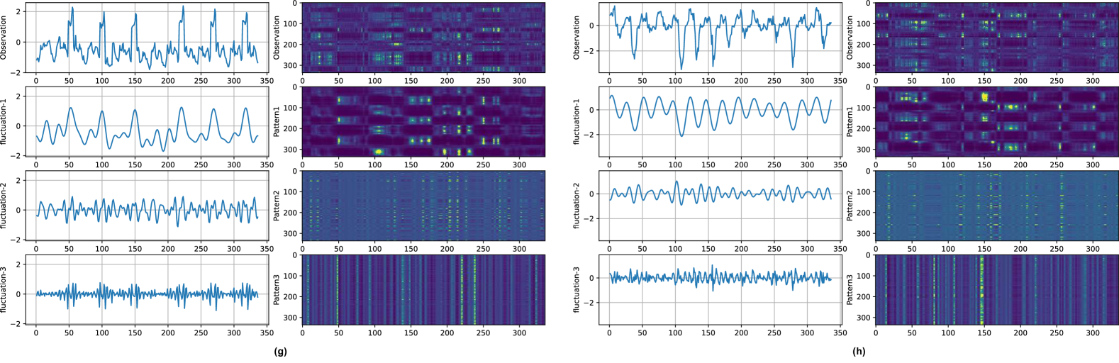
Figure 10: Visualization of the decomposition algorithm on the ETTm1 dataset. Additionally, we present the point-wise attention scores calculated on the observed sequence and the three decomposed sequences.

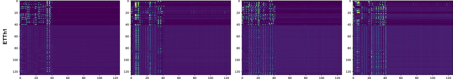
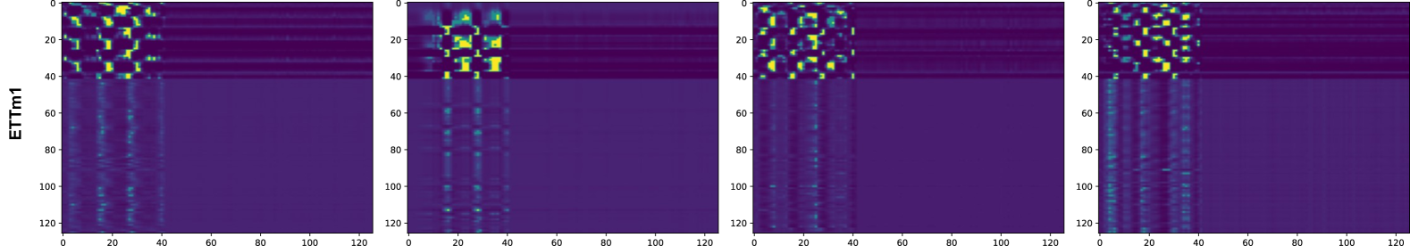
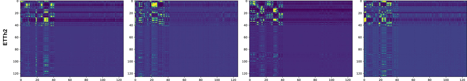
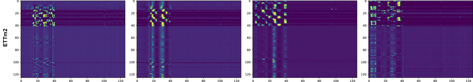
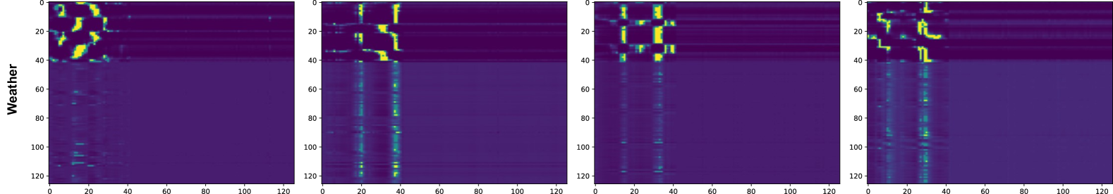
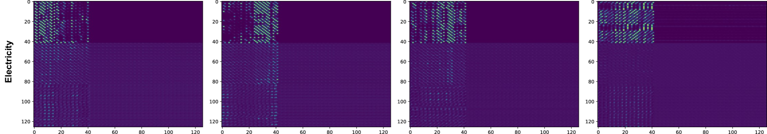
Figure 11: Attention scores among different fluctuation patterns were calculated and visualized in the forecasting task.

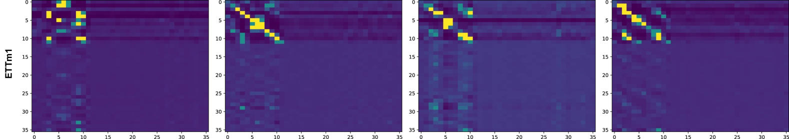
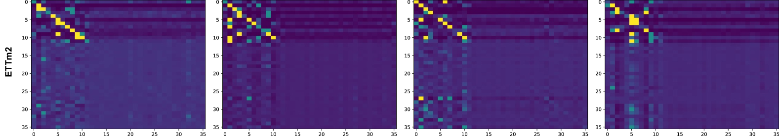
Figure 12: Attention scores among different fluctuation patterns were calculated and visualized in the imputation task.

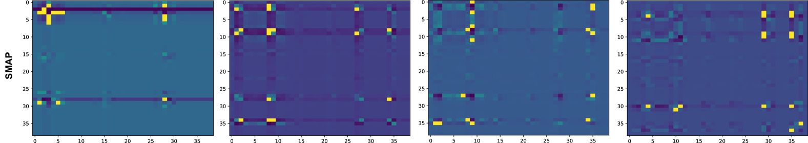
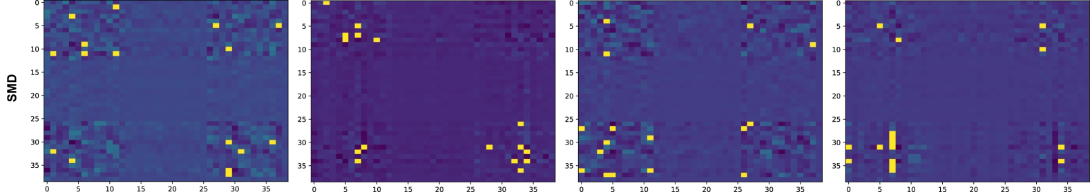
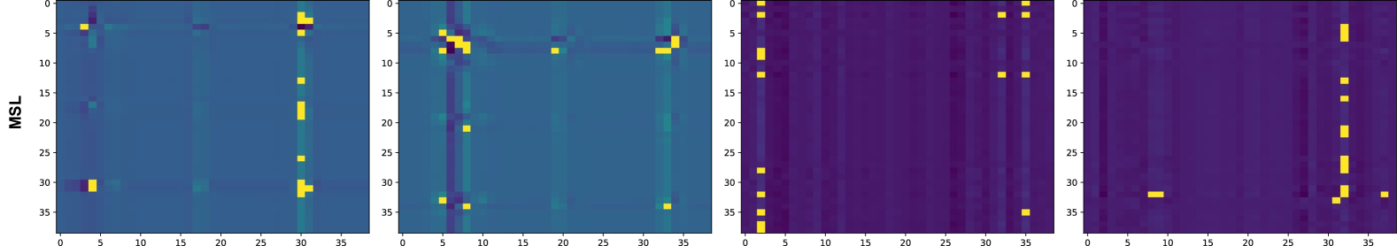
Figure 13: Attention scores among different fluctuation patterns were calculated and visualized in the anomaly detection task.

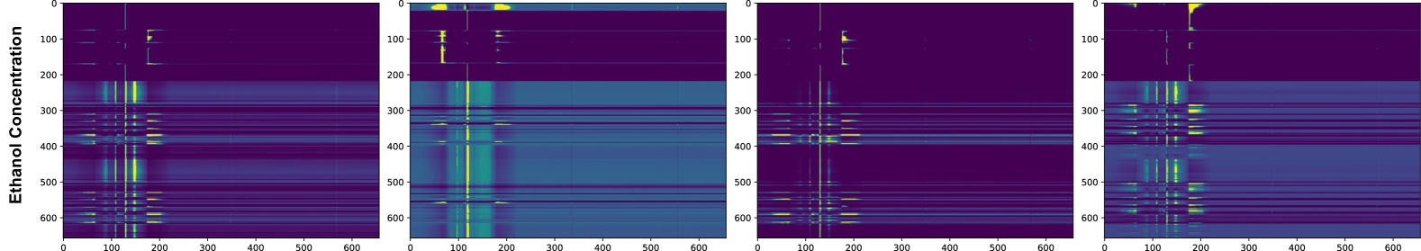
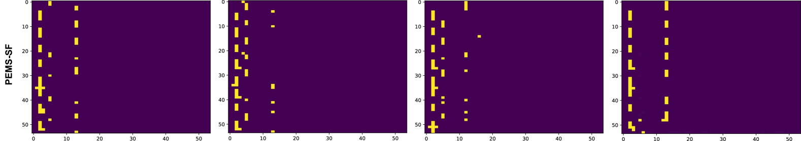
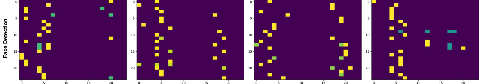
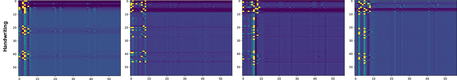
Figure 14: Attention scores among different fluctuation patterns were calculated and visualized in the classification task.

Appendix G Full Results

Due to the space limitation of the main text, we place the full results of all experiments in the following: long-term forecasting under full-shot setting in Table 12, long-term forecasting under few-shot setting in Table 13, long-term forecasting under zero-shot setting in Table 14, univariate short-term forecasting in Table 15, multivariate short-term forecasting in Table 16, anomaly detection in Table 17 and classification in Table 18. In addition, the complete ablation experiments of the enhancement strategy and the original baseline in the long-term forecasting task in Table 19

Table 12: Comparison of the complete performance with diverse prediction length on full-data long-term forecasting task. Avg is averaged from all four prediction lengths, that $\{96,192,336,720\}$. We boldface the best performance.

Models		Pets		TimeMixer		iTransformer		PatchTST		Crossformer		TiDE		TimesNet		DLinear		SCINet		FEDformer		Stationary		Autoformer
		(Ours)		[2024b]		[2024]		[2023]		[2021]		[2023]		[2023]		[2023]		[2021a]		[2022a]		[2022]		[2021]
Metric		MSE	MAE	MSE	MAE	MSE	MAE	MSE	MAE	MSE	MAE	MSE	MAE	MSE	MAE	MSE	MAE	MSE	MAE	MSE	MAE	MSE	MAE	MSE	MAE
Weather	96	0.146	0.194	0.163	0.209	0.174	0.214	0.186	0.227	0.195	0.271	0.202	0.261	0.172	0.220	0.195	0.252	0.221	0.306	0.217	0.296	0.173	0.223	0.266	0.336
	192	0.187	0.232	0.208	0.250	0.221	0.254	0.234	0.265	0.209	0.277	0.242	0.298	0.219	0.261	0.237	0.295	0.261	0.340	0.276	0.336	0.245	0.285	0.307	0.367
	336	0.237	0.272	0.251	0.287	0.278	0.296	0.284	0.301	0.273	0.332	0.287	0.335	0.280	0.306	0.282	0.331	0.309	0.378	0.339	0.380	0.321	0.338	0.359	0.395
	720	0.306	0.322	0.339	0.341	0.358	0.347	0.356	0.349	0.379	0.401	0.351	0.386	0.365	0.359	0.345	0.382	0.377	0.427	0.403	0.428	0.414	0.410	0.419	0.428
	Avg	0.219	0.255	0.240	0.271	0.258	0.278	0.265	0.285	0.264	0.320	0.271	0.320	0.259	0.287	0.265	0.315	0.292	0.363	0.309	0.360	0.288	0.314	0.338	0.382
Solar-Energy	96	0.167	0.229	0.189	0.259	0.203	0.237	0.265	0.323	0.232	0.302	0.312	0.399	0.373	0.358	0.290	0.378	0.237	0.344	0.286	0.341	0.321	0.380	0.456	0.446
	192	0.184	0.237	0.222	0.283	0.233	0.261	0.288	0.332	0.371	0.410	0.339	0.416	0.397	0.376	0.320	0.398	0.280	0.380	0.291	0.337	0.346	0.369	0.588	0.561
	336	0.197	0.252	0.231	0.292	0.248	0.273	0.301	0.339	0.495	0.515	0.368	0.430	0.420	0.380	0.353	0.415	0.304	0.389	0.354	0.416	0.357	0.387	0.595	0.588
	720	0.202	0.258	0.223	0.285	0.249	0.275	0.295	0.336	0.526	0.542	0.370	0.425	0.420	0.381	0.357	0.413	0.308	0.388	0.380	0.437	0.375	0.424	0.733	0.633
	Avg	0.187	0.244	0.216	0.280	0.233	0.262	0.287	0.333	0.406	0.442	0.347	0.417	0.403	0.374	0.330	0.401	0.282	0.375	0.328	0.383	0.350	0.390	0.586	0.557
Electricity	96	0.140	0.235	0.153	0.247	0.148	0.240	0.190	0.296	0.219	0.314	0.237	0.329	0.168	0.272	0.210	0.302	0.247	0.345	0.193	0.308	0.169	0.273	0.201	0.317
	192	0.158	0.250	0.166	0.256	0.162	0.253	0.199	0.304	0.231	0.322	0.236	0.330	0.184	0.322	0.210	0.305	0.257	0.355	0.201	0.315	0.182	0.286	0.222	0.334
	336	0.179	0.271	0.185	0.277	0.178	0.269	0.217	0.319	0.246	0.337	0.249	0.344	0.198	0.300	0.223	0.319	0.269	0.369	0.214	0.329	0.200	0.304	0.231	0.443
	720	0.214	0.299	0.225	0.310	0.225	0.317	0.258	0.352	0.280	0.363	0.284	0.373	0.220	0.320	0.258	0.350	0.299	0.390	0.246	0.355	0.222	0.321	0.254	0.361
	Avg	0.173	0.264	0.182	0.272	0.178	0.270	0.216	0.318	0.244	0.334	0.251	0.344	0.192	0.304	0.225	0.319	0.268	0.365	0.214	0.327	0.193	0.296	0.227	0.338
Traffic	96	0.375	0.259	0.462	0.285	0.395	0.268	0.526	0.347	0.644	0.429	0.805	0.493	0.593	0.321	0.650	0.396	0.788	0.499	0.587	0.366	0.612	0.338	0.613	0.388
	192	0.386	0.261	0.473	0.296	0.417	0.276	0.522	0.332	0.665	0.431	0.756	0.474	0.617	0.336	0.598	0.370	0.789	0.505	0.604	0.373	0.613	0.340	0.616	0.382
	336	0.408	0.270	0.498	0.296	0.433	0.283	0.517	0.334	0.674	0.420	0.762	0.477	0.629	0.336	0.605	0.373	0.797	0.508	0.621	0.383	0.618	0.328	0.622	0.337
	720	0.441	0.288	0.506	0.313	0.467	0.302	0.552	0.352	0.683	0.424	0.719	0.449	0.640	0.350	0.645	0.394	0.841	0.523	0.626	0.382	0.653	0.355	0.660	0.408
	Avg	0.403	0.269	0.484	0.297	0.428	0.282	0.529	0.341	0.667	0.426	0.760	0.473	0.620	0.336	0.625	0.383	0.804	0.509	0.610	0.376	0.624	0.340	0.628	0.379
Exchange	96	0.083	0.204	0.090	0.235	0.086	0.206	0.088	0.205	0.256	0.367	0.094	0.218	0.107	0.234	0.088	0.218	0.267	0.396	0.148	0.278	0.111	0.237	0.197	0.323
	192	0.179	0.319	0.187	0.343	0.177	0.299	0.176	0.299	0.470	0.509	0.184	0.307	0.226	0.344	0.176	0.315	0.351	0.459	0.271	0.315	0.219	0.335	0.300	0.369
	336	0.350	0.460	0.353	0.473	0.331	0.417	0.301	0.397	1.268	0.883	0.349	0.431	0.367	0.448	0.313	0.427	1.324	0.853	0.460	0.427	0.421	0.476	0.509	0.524
	720	0.921	0.765	0.934	0.761	0.847	0.691	0.901	0.714	1.767	1.068	0.852	0.698	0.964	0.746	0.839	0.695	1.058	0.797	1.195	0.695	1.092	0.769	1.447	0.941
	Avg	0.383	0.437	0.391	0.453	0.360	0.403	0.367	0.404	0.940	0.707	0.370	0.413	0.416	0.443	0.354	0.414	0.750	0.626	0.519	0.429	0.461	0.454	0.613	0.539
ETTh1	96	0.371	0.392	0.375	0.400	0.386	0.405	0.460	0.447	0.423	0.448	0.479	0.464	0.384	0.402	0.397	0.412	0.654	0.599	0.395	0.424	0.513	0.491	0.449	0.459
	192	0.409	0.414	0.429	0.421	0.441	0.512	0.477	0.429	0.471	0.474	0.525	0.492	0.436	0.429	0.446	0.441	0.719	0.631	0.469	0.470	0.534	0.504	0.500	0.482
	336	0.432	0.440	0.484	0.458	0.487	0.458	0.546	0.496	0.570	0.546	0.565	0.515	0.491	0.469	0.489	0.467	0.778	0.659	0.530	0.499	0.588	0.535	0.521	0.496
	720	0.448	0.459	0.498	0.482	0.503	0.491	0.544	0.517	0.653	0.621	0.594	0.558	0.521	0.500	0.513	0.510	0.836	0.699	0.598	0.544	0.643	0.616	0.514	0.512
	Avg	0.415	0.426	0.447	0.440	0.454	0.447	0.516	0.484	0.529	0.522	0.541	0.507	0.458	0.450	0.461	0.457	0.747	0.647	0.498	0.484	0.570	0.537	0.496	0.487
ETTh2	96	0.292	0.352	0.289	0.341	0.297	0.349	0.308	0.355	0.745	0.584	0.400	0.440	0.340	0.374	0.340	0.394	0.707	0.621	0.358	0.397	0.476	0.458	0.346	0.388
	192	0.352	0.390	0.372	0.392	0.380	0.400	0.393	0.405	0.877	0.656	0.528	0.509	0.402	0.414	0.482	0.479	0.860	0.689	0.429	0.439	0.512	0.493	0.456	0.452
	336	0.380	0.410	0.386	0.414	0.428	0.432	0.427	0.436	1.043	0.731	0.643	0.571	0.452	0.452	0.591	0.541	1.000	0.744	0.496	0.487	0.552	0.551	0.482	0.486
	720	0.418	0.440	0.412	0.434	0.427	0.445	0.436	0.450	1.104	0.763	0.874	0.679	0.462	0.468	0.839	0.661	1.249	0.838	0.463	0.474	0.562	0.560	0.515	0.511
	Avg	0.360	0.398	0.364	0.395	0.383	0.407	0.391	0.411	0.942	0.684	0.611	0.550	0.414	0.427	0.563	0.519	0.954	0.723	0.437	0.449	0.526	0.516	0.450	0.459
ETTm1	96	0.291	0.344	0.320	0.357	0.334	0.368	0.352	0.374	0.404	0.426	0.364	0.387	0.338	0.375	0.346	0.374	0.418	0.438	0.379	0.419	0.386	0.398	0.505	0.475
	192	0.333	0.371	0.361	0.381	0.390	0.393	0.374	0.387	0.450	0.451	0.398	0.404	0.374	0.387	0.382	0.391	0.439	0.450	0.426	0.441	0.459	0.444	0.553	0.496
	336	0.366	0.390	0.390	0.404	0.426	0.420	0.421	0.414	0.532	0.515	0.428	0.425	0.410	0.411	0.415	0.415	0.490	0.485	0.445	0.459	0.495	0.464	0.621	0.537
	720	0.413	0.421	0.454	0.441	0.491	0.459	0.462	0.449	0.666	0.589	0.487	0.461	0.478	0.450	0.473	0.451	0.595	0.550	0.543	0.490	0.585	0.516	0.671	0.561
	Avg	0.351	0.382	0.381	0.395	0.407	0.410	0.406	0.407	0.513	0.495	0.419	0.419	0.400	0.406	0.404	0.408	0.485	0.481	0.448	0.452	0.481	0.456	0.588	0.517
ETTm2	96	0.167	0.256	0.175	0.258	0.180	0.264	0.183	0.270	0.287	0.366	0.207	0.305	0.187	0.267	0.193	0.293	0.286	0.377	0.203	0.287	0.192	0.274	0.255	0.339
	192	0.220	0.282	0.237	0.299	0.250	0.309	0.255	0.314	0.414	0.492	0.290	0.364	0.249	0.309	0.284	0.361	0.399	0.445	0.269	0.328	0.280	0.339	0.281	0.340
	336	0.279	0.325	0.298	0.340	0.311	0.348	0.309	0.347	0.597	0.542	0.377	0.422	0.321	0.351	0.382	0.429	0.637	0.591	0.325	0.366	0.334	0.361	0.339	0.372
	720	0.354	0.378	0.391	0.396	0.412	0.407	0.412	0.404	1.730	1.042	0.558	0.524	0.408	0.403	0.558	0.525	0.960	0.735	0.421	0.415	0.417	0.413	0.433	0.432
	Avg	0.255	0.310	0.275	0.323	0.288	0.332	0.290	0.334	0.757	0.610	0.358	0.404	0.291	0.333	0.354	0.402	0.954	0.723	0.305	0.349	0.306	0.347	0.327	0.371
$1^{\text{st}}$ Count		67		13		0		0		0		0		0		0		0		0		0		0

Table 13: Comparison of the complete performance with diverse prediction length on few-data (10% data) long-term forecasting task. Avg is averaged from all four prediction lengths, that $\{96,192,336,720\}$. We boldface the best performance.

Models		Pets		TimeMixer		iTransformer		TiDE		DLinear		PatchTST		TimesNet		FEDformer		Autoformer		Stationary		ETSformer		LightTS
		(Ours)		[2024b]		[2024]		[2023]		[2023]		[2023]		[2023]		[2022a]		[2021]		[2022]		[2022]		[2023]
Metric		MSE	MAE	MSE	MAE	MSE	MAE	MSE	MAE	MSE	MAE	MSE	MAE	MSE	MAE	MSE	MAE	MSE	MAE	MSE	MAE	MSE	MAE	MSE	MAE
Weather	96	0.150	0.200	0.159	0.212	0.191	0.250	0.163	0.220	0.171	0.224	0.165	0.215	0.184	0.230	0.188	0.253	0.221	0.297	0.192	0.234	0.199	0.272	0.217	0.269
	192	0.196	0.242	0.207	0.257	0.249	0.302	0.213	0.266	0.215	0.263	0.210	0.257	0.245	0.283	0.250	0.304	0.270	0.322	0.269	0.295	0.279	0.332	0.259	0.304
	336	0.248	0.283	0.262	0.300	0.315	0.353	0.270	0.311	0.258	0.299	0.259	0.297	0.305	0.321	0.312	0.346	0.320	0.351	0.370	0.357	0.356	0.386	0.303	0.334
	720	0.322	0.335	0.340	0.355	0.409	0.418	0.350	0.368	0.320	0.346	0.332	0.346	0.381	0.371	0.387	0.393	0.390	0.396	0.441	0.405	0.437	0.448	0.377	0.382
	Avg	0.229	0.265	0.242	0.281	0.291	0.331	0.249	0.291	0.241	0.283	0.242	0.279	0.279	0.301	0.284	0.324	0.300	0.342	0.318	0.323	0.318	0.360	0.289	0.322
Electricity	96	0.132	0.231	0.152	0.250	0.196	0.304	0.160	0.261	0.150	0.253	0.140	0.238	0.299	0.373	0.231	0.323	0.261	0.348	0.420	0.466	0.599	0.587	0.350	0.425
	192	0.147	0.241	0.170	0.261	0.219	0.317	0.178	0.272	0.164	0.264	0.160	0.255	0.305	0.379	0.261	0.356	0.338	0.406	0.411	0.459	0.620	0.598	0.376	0.448
	336	0.165	0.260	0.190	0.281	0.245	0.342	0.200	0.294	0.181	0.282	0.180	0.276	0.319	0.391	0.360	0.445	0.410	0.474	0.434	0.473	0.662	0.619	0.428	0.485
	720	0.203	0.293	0.234	0.317	0.302	0.386	0.246	0.331	0.223	0.321	0.241	0.323	0.369	0.426	0.530	0.585	0.715	0.685	0.510	0.521	0.757	0.664	0.611	0.597
	Avg	0.162	0.256	0.187	0.277	0.241	0.337	0.196	0.289	0.180	0.280	0.180	0.273	0.323	0.392	0.346	0.427	0.431	0.478	0.444	0.480	0.660	0.617	0.441	0.489
Traffic	96	0.385	0.265	0.445	0.286	0.573	0.349	0.466	0.299	0.419	0.298	0.403	0.289	0.719	0.416	0.639	0.400	0.672	0.405	1.412	0.802	1.643	0.855	1.157	0.636
	192	0.396	0.271	0.457	0.293	0.589	0.357	0.479	0.306	0.434	0.305	0.415	0.296	0.748	0.428	0.637	0.416	0.727	0.424	1.419	0.806	1.641	0.854	1.207	0.661
	336	0.412	0.279	0.476	0.301	0.613	0.368	0.498	0.315	0.449	0.313	0.426	0.304	0.853	0.471	0.655	0.427	0.749	0.454	1.443	0.815	1.711	0.878	1.334	0.713
	720	0.433	0.292	0.500	0.315	0.644	0.385	0.524	0.330	0.484	0.336	0.474	0.331	1.485	0.825	0.722	0.456	0.847	0.499	1.539	0.837	2.660	1.157	1.292	0.726
	Avg	0.406	0.277	0.469	0.299	0.604	0.365	0.491	0.313	0.447	0.313	0.430	0.305	0.951	0.535	0.663	0.425	0.749	0.446	1.453	0.815	1.914	0.936	1.248	0.684
ETTh1	96	0.400	0.414	0.550	0.482	0.457	0.553	0.528	0.496	0.492	0.495	0.516	0.485	0.861	0.628	0.512	0.499	0.613	0.552	0.918	0.639	1.112	0.806	1.298	0.838
	192	0.439	0.436	0.603	0.507	0.502	0.582	0.580	0.522	0.565	0.538	0.598	0.524	0.797	0.593	0.624	0.555	0.722	0.598	0.915	0.629	1.155	0.823	1.322	0.854
	336	0.460	0.451	0.632	0.525	0.526	0.602	0.607	0.540	0.721	0.622	0.657	0.550	0.941	0.648	0.691	0.574	0.750	0.619	0.939	0.644	1.179	0.832	1.347	0.870
	720	0.484	0.486	0.665	0.565	0.553	0.649	0.639	0.582	0.986	0.743	0.762	0.610	0.877	0.641	0.728	0.614	0.721	0.616	0.887	0.645	1.273	0.874	1.534	0.947
	Avg	0.446	0.447	0.613	0.520	0.510	0.597	0.589	0.535	0.691	0.600	0.633	0.542	0.869	0.628	0.639	0.561	0.702	0.596	0.915	0.639	1.180	0.834	1.375	0.877
ETTh2	96	0.288	0.349	0.324	0.380	0.367	0.404	0.319	0.361	0.357	0.411	0.353	0.389	0.378	0.409	0.382	0.416	0.413	0.451	0.389	0.411	0.678	0.619	2.022	1.006
	192	0.359	0.395	0.404	0.430	0.458	0.458	0.397	0.409	0.569	0.519	0.403	0.414	0.490	0.467	0.478	0.474	0.474	0.477	0.473	0.455	0.785	0.666	2.329	1.104
	336	0.376	0.409	0.423	0.445	0.479	0.474	0.416	0.423	0.671	0.572	0.426	0.441	0.537	0.494	0.504	0.501	0.547	0.543	0.507	0.480	0.839	0.694	2.453	1.122
	720	0.403	0.438	0.454	0.477	0.514	0.507	0.446	0.453	0.824	0.648	0.477	0.480	0.510	0.491	0.499	0.509	0.516	0.523	0.477	0.472	1.273	0.874	3.816	1.407
	Avg	0.357	0.398	0.402	0.433	0.455	0.461	0.395	0.412	0.605	0.538	0.415	0.431	0.479	0.465	0.466	0.475	0.488	0.499	0.462	0.455	0.894	0.713	2.655	1.160
ETTm1	96	0.297	0.348	0.409	0.419	0.412	0.469	0.357	0.416	0.352	0.392	0.410	0.419	0.583	0.501	0.578	0.518	0.774	0.614	0.761	0.568	0.911	0.688	0.921	0.682
	192	0.333	0.371	0.458	0.447	0.462	0.500	0.400	0.444	0.382	0.412	0.437	0.434	0.630	0.528	0.617	0.546	0.754	0.592	0.781	0.574	0.955	0.703	0.957	0.701
	336	0.365	0.390	0.502	0.469	0.506	0.525	0.438	0.466	0.419	0.434	0.476	0.454	0.725	0.568	0.998	0.775	0.869	0.677	0.803	0.587	0.991	0.719	0.998	0.716
	720	0.420	0.424	0.578	0.510	0.583	0.571	0.504	0.507	0.490	0.477	0.681	0.556	0.769	0.549	0.693	0.579	0.810	0.630	0.844	0.581	1.062	0.747	1.007	0.719
	Avg	0.354	0.383	0.487	0.461	0.491	0.516	0.425	0.458	0.411	0.429	0.501	0.466	0.677	0.537	0.722	0.605	0.802	0.628	0.797	0.578	0.980	0.714	0.971	0.705
ETTm2	96	0.170	0.260	0.203	0.297	0.244	0.334	0.206	0.300	0.213	0.303	0.191	0.274	0.212	0.285	0.291	0.399	0.352	0.454	0.229	0.308	0.331	0.430	0.813	0.688
	192	0.227	0.299	0.270	0.342	0.326	0.384	0.276	0.346	0.278	0.345	0.252	0.317	0.270	0.323	0.307	0.379	0.694	0.691	0.291	0.343	0.400	0.464	1.008	0.768
	336	0.283	0.336	0.337	0.384	0.407	0.431	0.344	0.388	0.338	0.385	0.306	0.353	0.323	0.353	0.543	0.559	2.408	1.407	0.348	0.376	0.469	0.498	1.031	0.775
	720	0.365	0.389	0.435	0.445	0.524	0.499	0.443	0.450	0.436	0.440	0.433	0.427	0.474	0.449	0.712	0.614	1.913	1.166	0.461	0.438	0.589	0.557	1.096	0.791
	Avg	0.261	0.321	0.311	0.367	0.375	0.412	0.317	0.371	0.316	0.368	0.296	0.343	0.320	0.353	0.463	0.488	1.342	0.930	0.332	0.366	0.447	0.487	0.987	0.756
$1^{\text{st}}$ Count		69		1		0		0		0		0		0		0		0		0		0		0

Table 14: Comparison of the performance on Zero Shot Forecasting task. We present the model’s average performance across multiple prediction horizons.

Models	Pets		TimeMixer		LLMTime		PatchTST		TimesNet		iTransformer		TiDE
	(Ours)		[2024b]		[2024]		[2023]		[2023]		[2024]		[2023]
Metric	MSE	MAE	MSE	MAE	MSE	MAE	MSE	MAE	MSE	MAE	MSE	MAE	MSE	MAE
ETT h1$\rightarrow$h2	0.385	0.405	0.427	0.424	0.992	0.708	0.380	0.405	0.421	0.431	0.481	0.474	0.593	0.582
ETT h1$\rightarrow$m2	0.312	0.353	0.361	0.397	1.867	0.869	0.314	0.360	0.327	0.361	0.311	0.361	0.563	0.547
ETT h2$\rightarrow$h1	0.512	0.493	0.679	0.577	1.961	0.981	0.565	0.513	0.865	0.621	0.552	0.511	0.588	0.556
ETT m1$\rightarrow$h2	0.432	0.436	0.452	0.441	0.992	0.708	0.439	0.438	0.457	0.454	0.434	0.438	0.543	0.535
ETT m1$\rightarrow$m2	0.293	0.326	0.329	0.357	1.867	0.869	0.296	0.334	0.322	0.354	0.324	0.331	0.534	0.527
ETT m2$\rightarrow$m1	0.414	0.409	0.554	0.478	1.933	0.984	0.568	0.492	0.769	0.567	0.559	0.491	0.585	0.571

Table 15: Short-term forecasting results in the M4 dataset with a single variate. All prediction lengths are in $\left[6,48\right]$. A lower SMAPE, MASE or OWA indicates a better prediction.

Models			Pets	TimeMixer	iTransformer	TiDE	TimesNet	N-HiTS	N-BEATS	PatchTST	MICN	FiLM	LightTS	DLinear	FED.	Stationary	Auto.
			(Ours)	[2024b]	[2024]	[2023]	[2023]	[2022]	[2019]	[2023]	[2023]	[2022b]	[2023]	[2023]	[2022a]	[2022]	[2021]
Yearly		SMAPE	13.306	13.206	13.923	15.320	13.387	13.418	13.436	16.463	25.022	17.431	14.247	16.965	13.728	13.717	13.974
		MASE	2.910	2.916	3.214	3.540	2.996	3.045	3.043	3.967	7.162	4.043	3.109	4.283	3.048	3.078	3.134
		OWA	0.768	0.776	0.830	0.910	0.786	0.793	0.794	1.003	1.667	1.042	0.827	1.058	0.803	0.807	0.822
Quarterly		SMAPE	9.945	9.996	10.757	11.830	10.100	10.202	10.124	10.644	15.214	12.925	11.364	12.145	10.792	10.958	11.338
		MASE	1.147	1.166	1.283	1.410	1.182	1.194	1.169	1.278	1.963	1.664	1.328	1.520	1.283	1.325	1.365
		OWA	0.883	0.825	0.956	1.050	0.890	0.899	0.886	0.949	1.407	1.193	1.000	1.106	0.958	0.981	1.012
Monthly		SMAPE	12.398	12.605	13.796	15.180	12.670	12.791	12.677	13.399	16.943	15.407	14.014	13.514	14.260	13.917	13.958
		MASE	0.906	0.919	1.083	1.190	0.933	0.969	0.937	1.031	1.442	1.298	1.053	1.037	1.102	1.097	1.103
		OWA	0.844	0.869	0.987	1.090	0.878	0.899	0.880	0.949	1.265	1.144	0.981	0.956	1.012	0.998	1.002
Others		SMAPE	4.644	4.564	5.569	6.120	4.891	5.061	4.925	6.558	41.985	7.134	15.880	6.709	4.954	6.302	5.485
		MASE	3.014	3.115	3.940	4.330	3.302	3.216	3.391	4.511	62.734	5.09	11.434	4.953	3.264	4.064	3.865
		OWA	0.995	0.982	1.207	1.330	1.035	1.040	1.053	1.401	14.313	1.553	3.474	1.487	1.036	1.304	1.187
Weighted	Average	SMAPE	11.568	11.723	12.684	13.950	11.829	11.927	11.851	13.152	19.638	14.863	13.525	13.639	12.840	12.780	12.909
		MASE	1.471	1.559	1.764	1.940	1.585	1.613	1.559	1.945	5.947	2.207	2.111	2.095	1.701	1.756	1.771
		OWA	0.834	0.840	0.929	1.020	0.851	0.861	0.855	0.998	2.279	1.125	1.051	1.051	0.918	0.930	0.939

Table 16: Short-term forecasting results in the PEMS datasets with multiple variates. All input lengths are 96 and prediction lengths are 12. A lower MAE, MAPE or RMSE indicates a better prediction.

Models		Pets	TimeMixer	iTransformer	TiDE	SCINet	Crossformer	PatchTST	TimesNet	MICN	DLinear	FEDformer	Stationary	Autoformer
		(Ours)	[2024b]	[2024]	[2023]	[2021a]	[2021]	[2023]	[2023]	[2023]	[2023]	[2022a]	[2022]	[2021]
PEMS03	MAE	14.46	14.63	16.72	18.39	15.97	15.64	18.95	16.41	15.71	19.70	19.00	17.64	18.08
	MAPE	11.41	11.54	15.81	17.39	15.89	15.74	17.29	15.17	15.67	18.35	18.57	17.56	18.75
	RMSE	23.01	23.28	27.81	30.59	25.20	25.56	30.15	26.72	24.55	32.35	30.05	28.37	27.82
PEMS04	MAE	18.06	19.21	21.81	23.99	20.35	20.38	24.86	21.63	21.62	24.62	26.51	22.34	25.00
	MAPE	12.13	12.53	13.42	14.76	12.84	12.84	16.65	13.15	13.53	16.12	16.76	14.85	16.70
	RMSE	29.93	30.92	33.91	37.30	32.31	32.41	40.46	34.90	34.39	39.51	41.81	35.47	38.02
PEMS07	MAE	18.65	20.57	23.01	25.31	22.79	22.54	27.87	25.12	22.28	28.65	27.92	26.02	26.92
	MAPE	7.82	8.62	10.02	11.02	9.41	9.38	12.69	10.60	9.57	12.15	12.29	11.75	11.83
	RMSE	30.46	33.59	35.56	39.12	35.61	35.49	42.56	40.71	35.40	45.02	42.29	42.34	40.60
PEMS08	MAE	12.95	15.22	17.94	19.73	17.38	17.56	20.35	19.01	17.76	20.26	20.56	19.29	20.47
	MAPE	8.59	9.67	10.93	12.02	10.80	10.92	13.15	11.83	10.76	12.09	12.41	12.21	12.27
	RMSE	21.04	24.26	27.88	30.67	27.34	27.21	31.04	30.65	27.26	32.38	32.97	38.62	31.52

Table 17: Full results for the anomaly detection task. The P, R and F1 represent the precision, recall and F1-score (%) respectively. F1-score is the harmonic mean of precision and recall. A higher value of P, R and F1 indicates a better performance.

Datasets		SMD			MSL			SMAP			SWaT			PSM			Avg F1
Metrics		P	R	F1	P	R	F1	P	R	F1	P	R	F1	P	R	F1	(%)
LSTM	[1997]	78.52	65.47	71.41	78.04	86.22	81.93	91.06	57.49	70.48	78.06	91.72	84.34	69.24	99.53	81.67	77.97
Transformer	[2017]	83.58	76.13	79.56	71.57	87.37	78.68	89.37	57.12	69.70	68.84	96.53	80.37	62.75	96.56	76.07	76.88
LogTrans	[2019]	83.46	70.13	76.21	73.05	87.37	79.57	89.15	57.59	69.97	68.67	97.32	80.52	63.06	98.00	76.74	76.60
TCN	[2019]	84.06	79.07	81.49	75.11	82.44	78.60	86.90	59.23	70.45	76.59	95.71	85.09	54.59	99.77	70.57	77.24
Reformer	[2020]	82.58	69.24	75.32	85.51	83.31	84.40	90.91	57.44	70.40	72.50	96.53	82.80	59.93	95.38	73.61	77.31
Informer	[2021]	86.60	77.23	81.65	81.77	86.48	84.06	90.11	57.13	69.92	70.29	96.75	81.43	64.27	96.33	77.10	78.83
Anomaly Transformer	[2021]	88.91	82.23	85.49	79.61	87.37	83.31	91.85	58.11	71.18	72.51	97.32	83.10	68.35	94.72	79.40	80.50
Pyraformer	[2021b]	85.61	80.61	83.04	83.81	85.93	84.86	92.54	57.71	71.09	87.92	96.00	91.78	71.67	96.02	82.08	82.57
Autoformer	[2021]	88.06	82.35	85.11	77.27	80.92	79.05	90.40	58.62	71.12	89.85	95.81	92.74	99.08	88.15	93.29	84.26
LSSL	[2022]	78.51	65.32	71.31	77.55	88.18	82.53	89.43	53.43	66.90	79.05	93.72	85.76	66.02	92.93	77.20	76.74
Stationary	[2022]	88.33	81.21	84.62	68.55	89.14	77.50	89.37	59.02	71.09	68.03	96.75	79.88	97.82	96.76	97.29	82.08
DLinear	[2023]	83.62	71.52	77.10	84.34	85.42	84.88	92.32	55.41	69.26	80.91	95.30	87.52	98.28	89.26	93.55	82.46
ETSformer	[2022]	87.44	79.23	83.13	85.13	84.93	85.03	92.25	55.75	69.50	90.02	80.36	84.91	99.31	85.28	91.76	82.87
LightTS	[2023]	87.10	78.42	82.53	82.40	75.78	78.95	92.58	55.27	69.21	91.98	94.72	93.33	98.37	95.97	97.15	84.23
FEDformer	[2022a]	87.95	82.39	85.08	77.14	80.07	78.57	90.47	58.10	70.76	90.17	96.42	93.19	97.31	97.16	97.23	84.97
TimesNet	[2023]	88.66	83.14	85.81	83.92	86.42	85.15	92.52	58.29	71.52	86.76	97.32	91.74	98.19	96.76	97.47	86.34
TiDE	[2023]	76.00	63.00	68.91	84.00	60.00	70.18	88.00	50.00	64.00	98.00	63.00	76.73	93.00	92.00	92.50	74.46
iTransformer	[2024]	78.45	65.10	71.15	86.15	62.65	72.54	90.67	52.96	66.87	99.96	65.55	79.18	95.65	94.69	95.17	76.98
Pets	(Ours)	89.67	90.76	90.21	90.64	81.83	85.89	91.89	65.86	76.73	95.35	93.85	94.09	99.78	96.11	97.72	89.93

Table 18: Full results for the classification task. We report the classification accuracy (%) as the result. The standard deviation is within 0.1%.

Datasets/Models	Classical methods			RNN			TCN	Transformers										MLP			CNN
	DTW	XGBoost	Rocket	LSTM	LSTNet	LSSL	TCN	Trans.	Re.	In.	Pyra.	Auto.	Stat.	FED.	ETS.	Flow.	iTrans.	DLinear	LightTS.	TiDE	TimesNet	Pets
	[1994]	[2016]	[2019]	[1997]	[2018]	[2022]	[2019]	[2017]	[2020]	[2021]	[2021b]	[2021]	[2022]	[2022a]	[2022]	[2022]	[2024]	[2023]	[2023]	[2023]	[2023]	(Ours)
EthanolConcentration	32.3	43.7	45.2	32.3	39.9	31.1	28.9	32.7	31.9	31.6	30.8	31.6	32.7	28.1	31.2	33.8	28.1	32.6	29.7	27.1	35.7	36.9
FaceDetection	52.9	63.3	64.7	57.7	65.7	66.7	52.8	67.3	68.6	67.0	65.7	68.4	68.0	66.0	66.3	67.6	66.3	68.0	67.5	65.3	68.6	69.1
Handwriting	28.6	15.8	58.8	15.2	25.8	24.6	53.3	32.0	27.4	32.8	29.4	36.7	31.6	28.0	32.5	33.8	24.2	27.0	26.1	23.2	32.1	31.5
Heartbeat	71.7	73.2	75.6	72.2	77.1	72.7	75.6	76.1	77.1	80.5	75.6	74.6	73.7	73.7	71.2	77.6	75.6	75.1	75.1	74.6	78.0	76.5
JapaneseVowels	94.9	86.5	96.2	79.7	98.1	98.4	98.9	98.7	97.8	98.9	98.4	96.2	99.2	98.4	95.9	98.9	96.6	96.2	96.2	95.6	98.4	99.1
PEMS-SF	71.1	98.3	75.1	39.9	86.7	86.1	68.8	82.1	82.7	81.5	83.2	82.7	87.3	80.9	86.0	83.8	87.9	75.1	88.4	86.9	89.6	93.0
SelfRegulationSCP1	77.7	84.6	90.8	68.9	84.0	90.8	84.6	92.2	90.4	90.1	88.1	84.0	89.4	88.7	89.6	92.5	90.2	87.3	89.8	89.2	91.8	91.8
SelfRegulationSCP2	53.9	48.9	53.3	46.6	52.8	52.2	55.6	53.9	56.7	53.3	53.3	50.6	57.2	54.4	55.0	56.1	54.4	50.5	51.1	53.4	57.2	60.0
SpokenArabicDigits	96.3	69.6	71.2	31.9	100.0	100.0	95.6	98.4	97.0	100.0	99.6	100.0	100.0	100.0	100.0	98.8	96.0	81.4	100.0	95.0	99.0	99.3
UWaveGestureLibrary	90.3	75.9	94.4	41.2	87.8	85.9	88.4	85.6	85.6	85.6	83.4	85.9	87.5	85.3	85.0	86.6	85.9	82.1	80.3	84.9	85.3	89.6
Average Accuracy	67.0	66.0	72.5	48.6	71.8	70.9	70.3	71.9	71.5	72.1	70.8	71.1	72.7	70.7	71.0	73.0	70.5	67.5	70.4	69.5	73.6	74.7

Table 19: forecasting enhanced.

Methods		PatchTST [2023]						TimeMixer [2024b]						DLinear [2023]						TimesNet [2023]
Metric		Original		Enhance		Improve		Original		Enhance		Improve		Original		Enhance		Improve		Original		Enhance		Improve
		MSE	MAE	MSE	MAE	MSE	MAE	MSE	MAE	MSE	MAE	MSE	MAE	MSE	MAE	MSE	MAE	MSE	MAE	MSE	MAE	MSE	MAE	MSE	MAE
Weather	96	0.186	0.227	0.146	0.194	21.5%	14.5%	0.163	0.209	0.147	0.199	9.8%	4.8%	0.195	0.252	0.173	0.222	13.5%	11.9%	0.172	0.22	0.156	0.195	9.2%	11.4%
	192	0.234	0.265	0.187	0.232	20.1%	12.5%	0.208	0.250	0.190	0.242	8.7%	3.2%	0.237	0.295	0.215	0.258	10.6%	12.5%	0.219	0.261	0.201	0.231	8.7%	11.4%
	336	0.284	0.301	0.237	0.272	16.5%	9.6%	0.251	0.287	0.241	0.282	4.0%	1.7%	0.282	0.331	0.263	0.292	7.6%	11.8%	0.246	0.337	0.234	0.318	5.0%	5.5%
	720	0.356	0.349	0.306	0.322	14.0%	7.7%	0.339	0.341	0.319	0.333	5.9%	2.3%	0.345	0.382	0.330	0.338	4.4%	11.5%	0.365	0.359	0.345	0.339	5.5%	5.6%
	Avg	0.265	0.285	0.219	0.255	17.4%	10.5%	0.240	0.271	0.224	0.264	6.7%	2.6%	0.265	0.315	0.245	0.277	8.3%	12.1%	0.251	0.294	0.241	0.280	4.0%	4.7%
Solar-Energy	96	0.265	0.323	0.167	0.229	37.0%	29.1%	0.189	0.259	0.160	0.224	15.3%	13.5%	0.290	0.378	0.224	0.255	34.9%	32.5%	0.373	0.358	0.339	0.324	9.0%	9.6%
	192	0.288	0.332	0.184	0.237	36.1%	28.6%	0.222	0.283	0.189	0.252	14.9%	11.0%	0.320	0.398	0.256	0.274	28.8%	31.2%	0.397	0.376	0.368	0.341	7.2%	9.4%
	336	0.301	0.339	0.197	0.252	34.6%	25.7%	0.231	0.292	0.198	0.280	14.3%	4.1%	0.353	0.415	0.278	0.288	32.5%	30.6%	0.420	0.380	0.398	0.357	5.3%	6.0%
	720	0.295	0.336	0.202	0.258	31.5%	23.2%	0.223	0.285	0.206	0.250	7.6%	12.3%	0.357	0.413	0.278	0.287	35.4%	30.5%	0.420	0.381	0.392	0.352	6.7%	7.7%
	Avg	0.287	0.333	0.187	0.244	34.8%	26.7%	0.216	0.280	0.188	0.251	13.0%	10.4%	0.330	0.401	0.259	0.276	32.9%	31.2%	0.403	0.374	0.374	0.340	7.3%	9.1%
Electricity	96	0.190	0.296	0.150	0.245	21.1%	17.2%	0.153	0.247	0.128	0.223	16.3%	9.7%	0.210	0.302	0.161	0.257	23.3%	14.9%	0.168	0.272	0.161	0.261	4.3%	4.2%
	192	0.199	0.304	0.168	0.260	15.6%	14.5%	0.166	0.256	0.149	0.243	10.2%	5.1%	0.210	0.305	0.175	0.269	16.6%	11.8%	0.184	0.322	0.175	0.302	5.1%	6.2%
	336	0.217	0.319	0.179	0.271	17.5%	15.0%	0.185	0.277	0.166	0.259	10.3%	6.5%	0.223	0.319	0.192	0.286	13.9%	10.3%	0.198	0.299	0.178	0.266	9.9%	11.4%
	720	0.258	0.352	0.214	0.299	17.1%	15.1%	0.225	0.310	0.201	0.292	10.7%	5.8%	0.258	0.350	0.231	0.318	10.5%	9.1%	0.220	0.320	0.199	0.284	9.5%	11.1%
	Avg	0.216	0.318	0.178	0.269	17.6%	15.4%	0.182	0.272	0.161	0.254	11.5%	6.6%	0.225	0.319	0.189	0.283	16.0%	11.3%	0.193	0.304	0.172	0.270	10.7%	11.1%
Traffic	96	0.526	0.347	0.456	0.289	13.3%	16.7%	0.462	0.285	0.381	0.263	17.5%	7.7%	0.650	0.396	0.480	0.311	26.2%	21.5%	0.593	0.321	0.553	0.294	6.7%	8.5%
	192	0.522	0.332	0.465	0.291	10.9%	12.3%	0.473	0.296	0.402	0.276	15.0%	6.8%	0.598	0.370	0.494	0.317	17.4%	14.3%	0.617	0.336	0.572	0.305	7.3%	9.1%
	336	0.517	0.334	0.478	0.301	7.5%	9.9%	0.498	0.296	0.420	0.278	15.7%	6.1%	0.605	0.373	0.506	0.322	16.4%	13.7%	0.629	0.336	0.574	0.302	8.7%	10.1%
	720	0.552	0.352	0.511	0.318	7.4%	9.7%	0.506	0.313	0.453	0.294	10.5%	6.1%	0.645	0.394	0.536	0.343	16.9%	12.9%	0.640	0.350	0.596	0.327	6.9%	6.7%
	Avg	0.529	0.341	0.478	0.299	9.6%	12.3%	0.484	0.297	0.414	0.278	14.5%	6.4%	0.625	0.383	0.504	0.323	19.4%	15.7%	0.620	0.336	0.578	0.314	6.7%	6.6%
ETTh1	96	0.460	0.447	0.371	0.392	19.3%	12.3%	0.375	0.401	0.370	0.389	1.3%	2.5%	0.397	0.412	0.369	0.392	7.5%	4.9%	0.384	0.402	0.357	0.369	7.0%	8.2%
	192	0.512	0.477	0.409	0.414	20.1%	13.2%	0.429	0.421	0.405	0.416	5.6%	1.2%	0.446	0.441	0.403	0.412	10.0%	6.6%	0.436	0.429	0.413	0.404	5.3%	5.9%
	336	0.546	0.496	0.432	0.440	20.9%	11.3%	0.484	0.458	0.423	0.428	12.6%	6.6%	0.489	0.467	0.428	0.427	12.6%	8.6%	0.638	0.469	0.602	0.432	5.6%	7.9%
	720	0.544	0.517	0.448	0.459	17.6%	11.2%	0.498	0.482	0.448	0.451	10.0%	6.4%	0.513	0.510	0.437	0.459	15.3%	10.0%	0.521	0.498	0.475	0.453	8.8%	9.4%
	Avg	0.516	0.484	0.415	0.426	19.6%	12.0%	0.447	0.440	0.411	0.421	8.1%	4.3%	0.461	0.457	0.409	0.422	11.6%	7.7%	0.495	0.450	0.459	0.420	7.2%	6.7%
ETTh2	96	0.308	0.355	0.292	0.352	5.2%	0.8%	0.289	0.341	0.291	0.349	-0.7%	-2.3%	0.340	0.394	0.300	0.335	11.8%	14.9%	0.340	0.374	0.313	0.344	7.8%	7.9%
	192	0.393	0.405	0.352	0.390	10.4%	3.7%	0.372	0.392	0.347	0.386	6.7%	1.5%	0.482	0.479	0.362	0.377	24.9%	21.3%	0.402	0.414	0.387	0.395	3.7%	4.5%
	336	0.427	0.436	0.380	0.414	11.0%	5.0%	0.386	0.414	0.374	0.409	3.1%	1.2%	0.591	0.541	0.386	0.396	34.7%	26.8%	0.452	0.452	0.412	0.400	8.9%	11.4%
	720	0.436	0.450	0.418	0.440	4.1%	2.2%	0.412	0.434	0.417	0.449	-1.2%	-3.5%	0.839	0.661	0.457	0.424	45.5%	35.9%	0.462	0.468	0.425	0.419	8.0%	10.5%
	Avg	0.391	0.411	0.360	0.399	7.9%	2.9%	0.364	0.395	0.357	0.398	1.9%	-0.8%	0.563	0.519	0.376	0.383	33.2%	26.2%	0.414	0.427	0.392	0.397	5.4%	7.1%
ETTm1	96	0.352	0.374	0.291	0.344	17.3%	8.0%	0.320	0.357	0.294	0.349	8.1%	2.2%	0.346	0.374	0.297	0.340	15.3%	9.1%	0.338	0.375	0.321	0.347	5.0%	7.4%
	192	0.390	0.393	0.333	0.371	14.6%	5.6%	0.361	0.381	0.333	0.371	7.8%	2.6%	0.382	0.391	0.333	0.362	13.6%	7.4%	0.374	0.387	0.354	0.359	5.3%	7.2%
	336	0.421	0.414	0.366	0.390	13.1%	5.8%	0.390	0.404	0.363	0.391	6.9%	3.2%	0.415	0.415	0.362	0.378	13.6%	8.9%	0.410	0.411	0.383	0.375	6.5%	8.7%
	720	0.462	0.449	0.413	0.421	10.6%	6.2%	0.454	0.441	0.419	0.424	7.7%	3.9%	0.473	0.451	0.424	0.413	10.8%	8.4%	0.478	0.450	0.450	0.418	5.9%	7.2%
	Avg	0.406	0.407	0.351	0.382	13.5%	6.1%	0.381	0.395	0.352	0.384	7.6%	2.8%	0.404	0.408	0.354	0.373	13.1%	8.6%	0.401	0.406	0.373	0.377	6.7%	7.2%
ETTm2	96	0.183	0.270	0.167	0.256	8.7%	5.2%	0.175	0.258	0.173	0.262	1.1%	-1.6%	0.193	0.293	0.163	0.252	17.1%	14.0%	0.187	0.267	0.175	0.245	6.5%	8.3%
	192	0.255	0.314	0.220	0.282	13.7%	10.2%	0.237	0.299	0.234	0.305	1.3%	-2.0%	0.284	0.361	0.218	0.290	27.8%	19.7%	0.249	0.309	0.227	0.284	9.0%	8.2%
	336	0.309	0.347	0.279	0.325	9.7%	6.3%	0.298	0.340	0.281	0.336	5.7%	1.2%	0.382	0.429	0.272	0.325	36.9%	24.2%	0.321	0.351	0.302	0.332	5.9%	5.5%
	720	0.412	0.404	0.354	0.378	14.1%	6.4%	0.391	0.396	0.364	0.381	6.9%	3.9%	0.558	0.525	0.367	0.384	48.8%	26.9%	0.408	0.403	0.376	0.366	7.9%	9.1%
	Avg	0.290	0.334	0.255	0.310	12.1%	7.2%	0.275	0.323	0.263	0.319	4.4%	1.3%	0.354	0.402	0.255	0.313	36.0%	22.1%	0.291	0.333	0.265	0.297	8.8%	10.8%

Appendix H Showcases

To assess the performance of various models, we perform a qualitative comparison by visualizing the final dimension of the forecasting results derived from the test set of each dataset (Fig. 15, 16, 17, 18, 19, 20, 21). Among the various models, Pets exhibits superior performance.

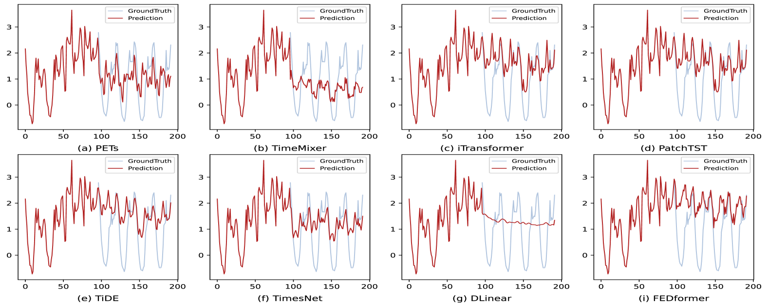
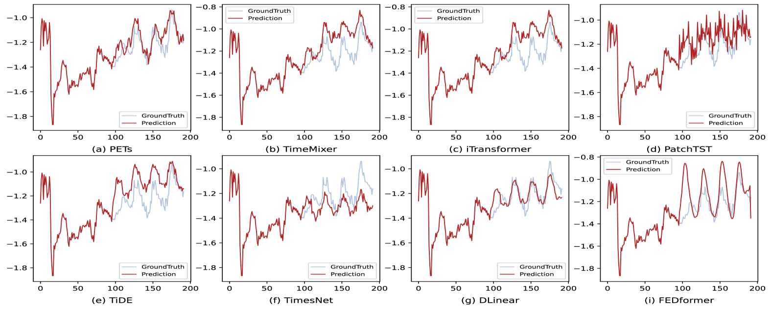
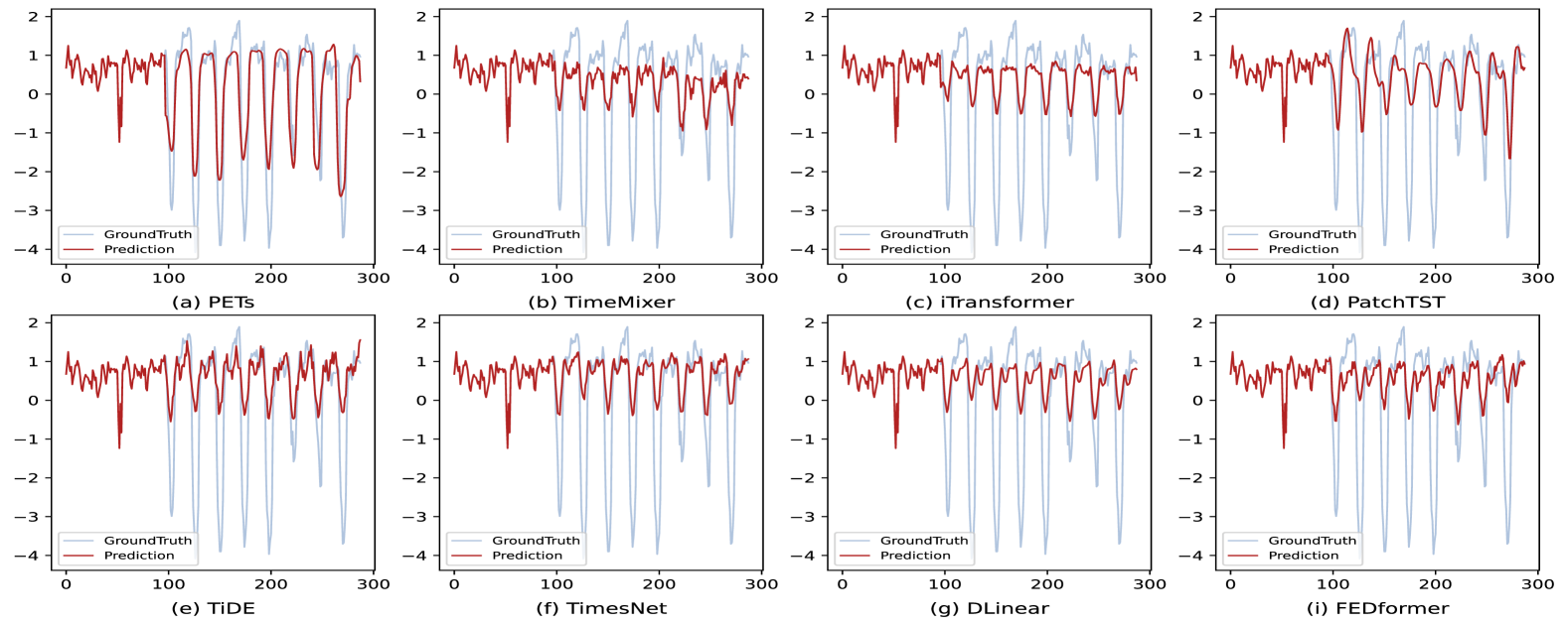
Figure 15: Prediction cases from ETTh1 by different models under the input-96-predict-96 settings.

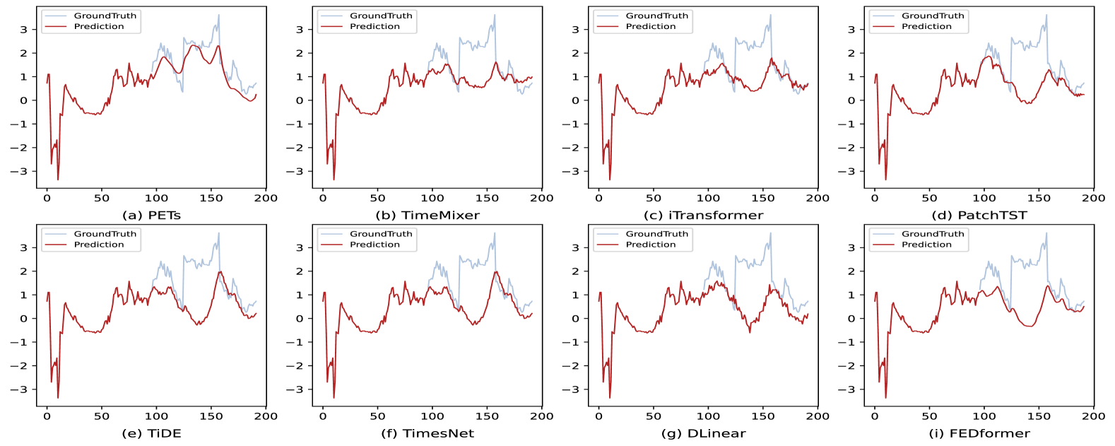
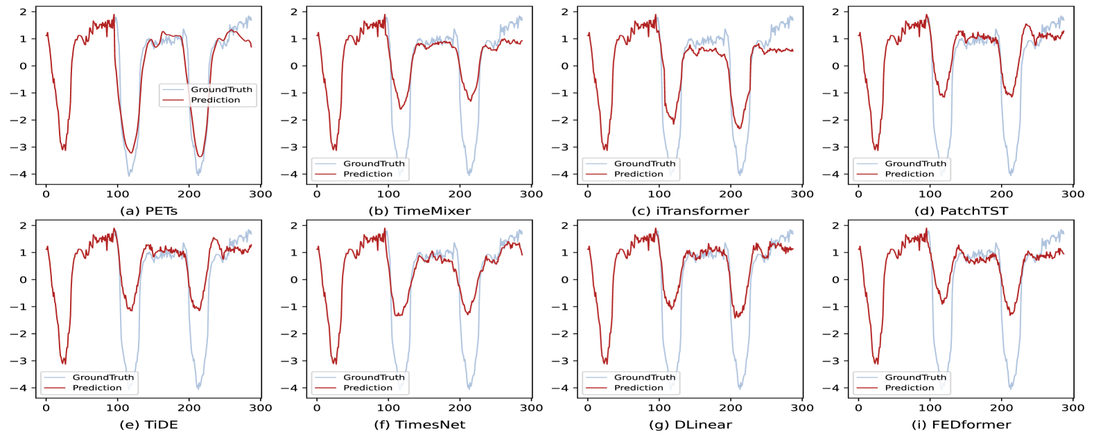
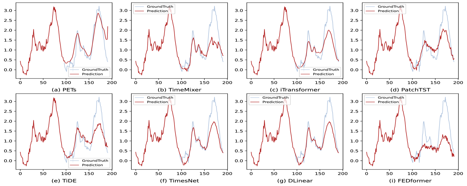
Figure 16: Prediction cases from ETTm1 by different models under the input-96-predict-96 settings.

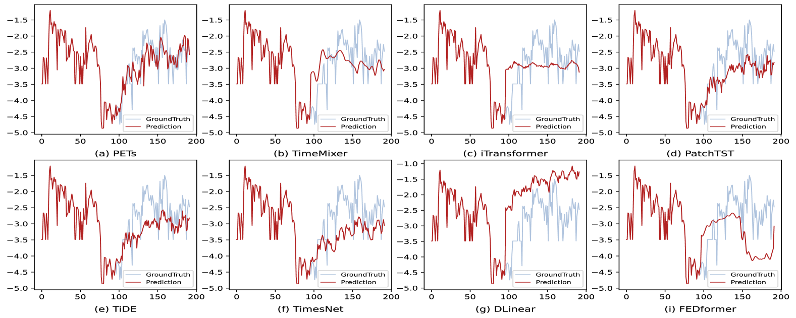
Figure 17: Prediction cases from ETTh2 by different models under the input-96-predict-96 settings.

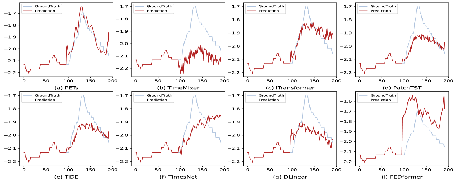
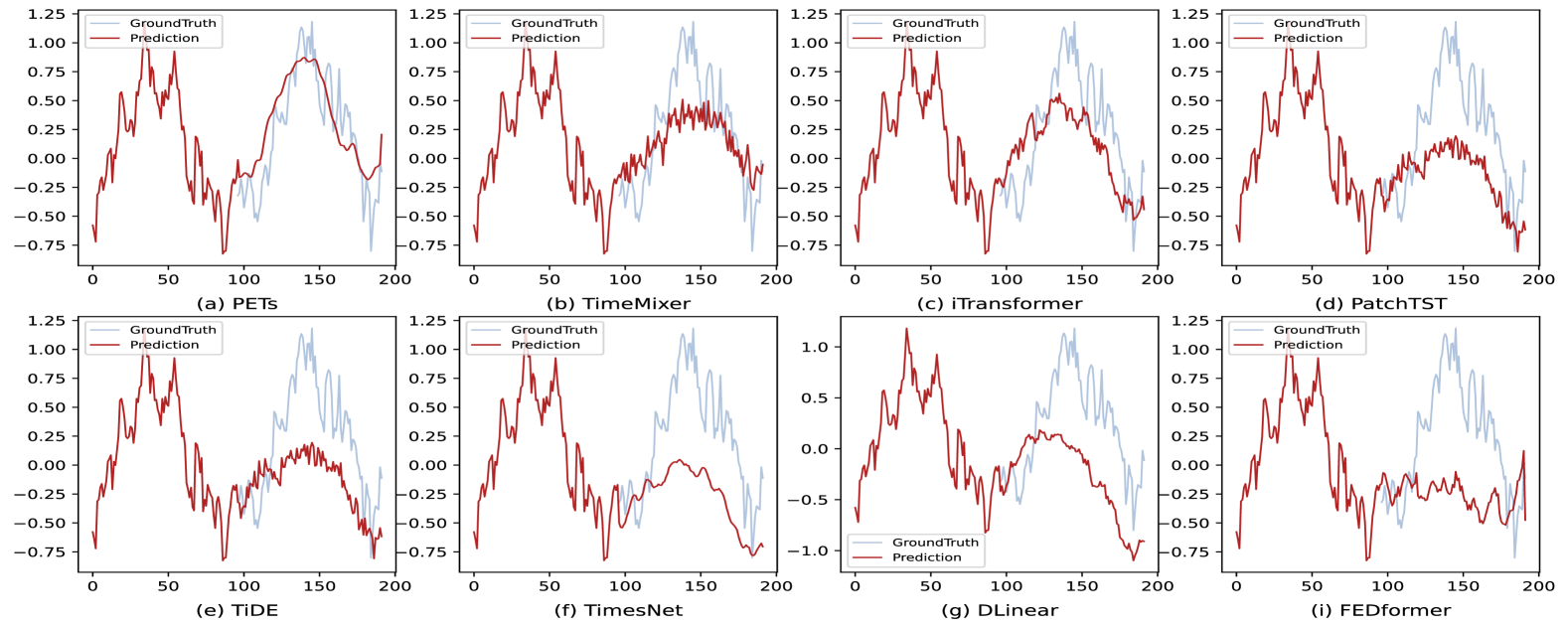
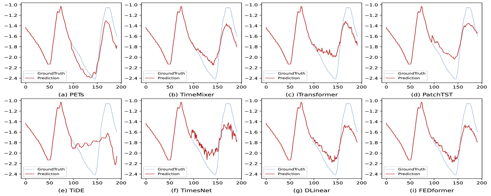
Figure 18: Prediction cases from ETTm2 by different models under the input-96-predict-96 settings.

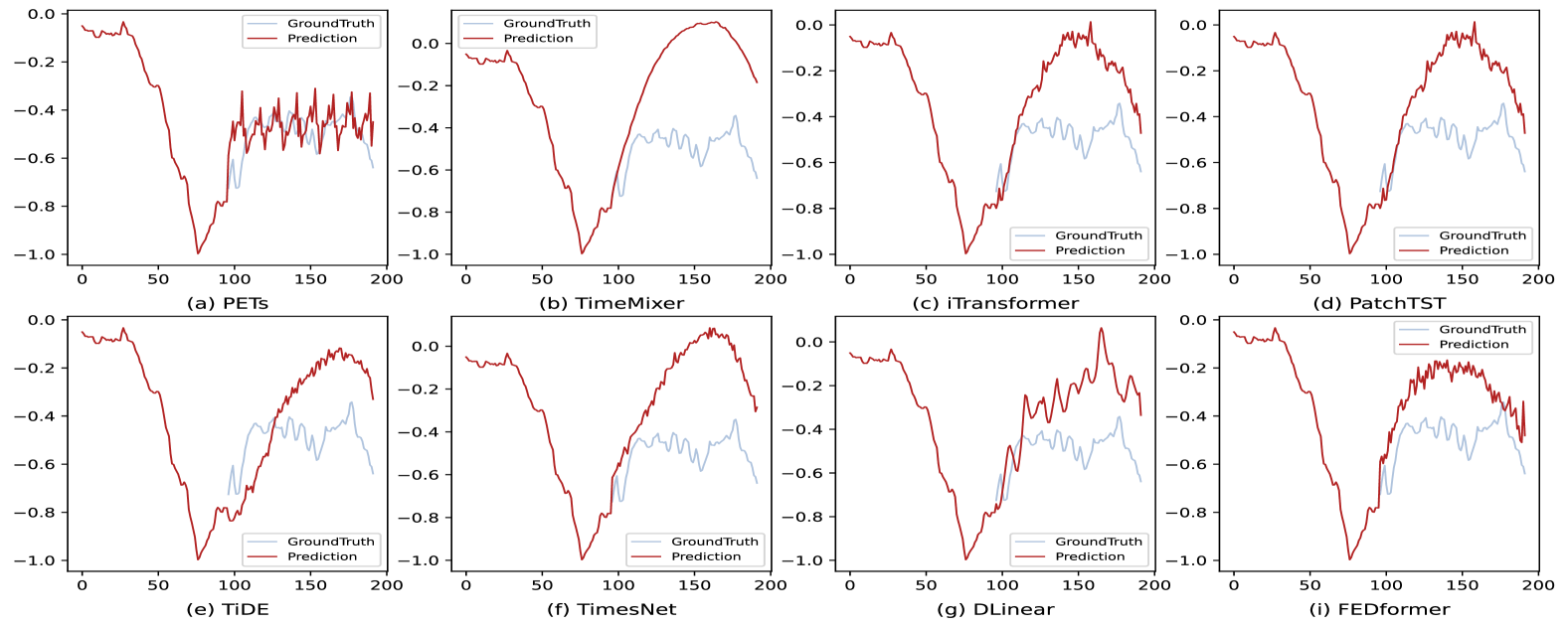
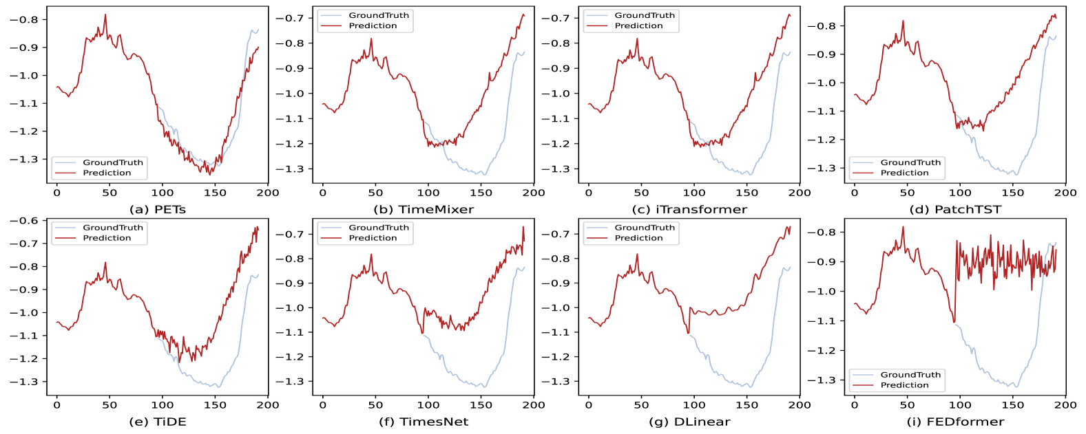
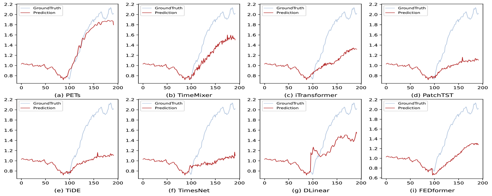
Figure 19: Prediction cases from Weather by different models under the input-96-predict-96 settings.

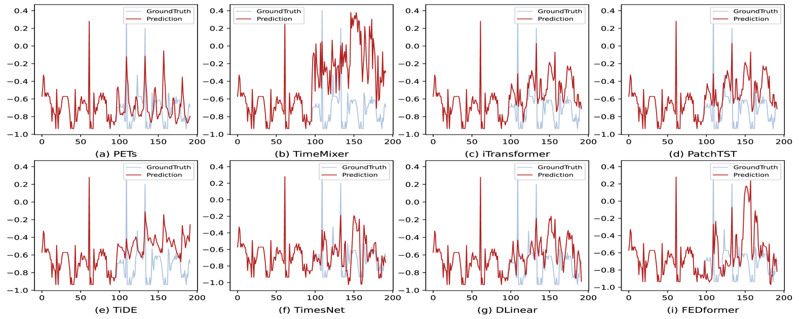
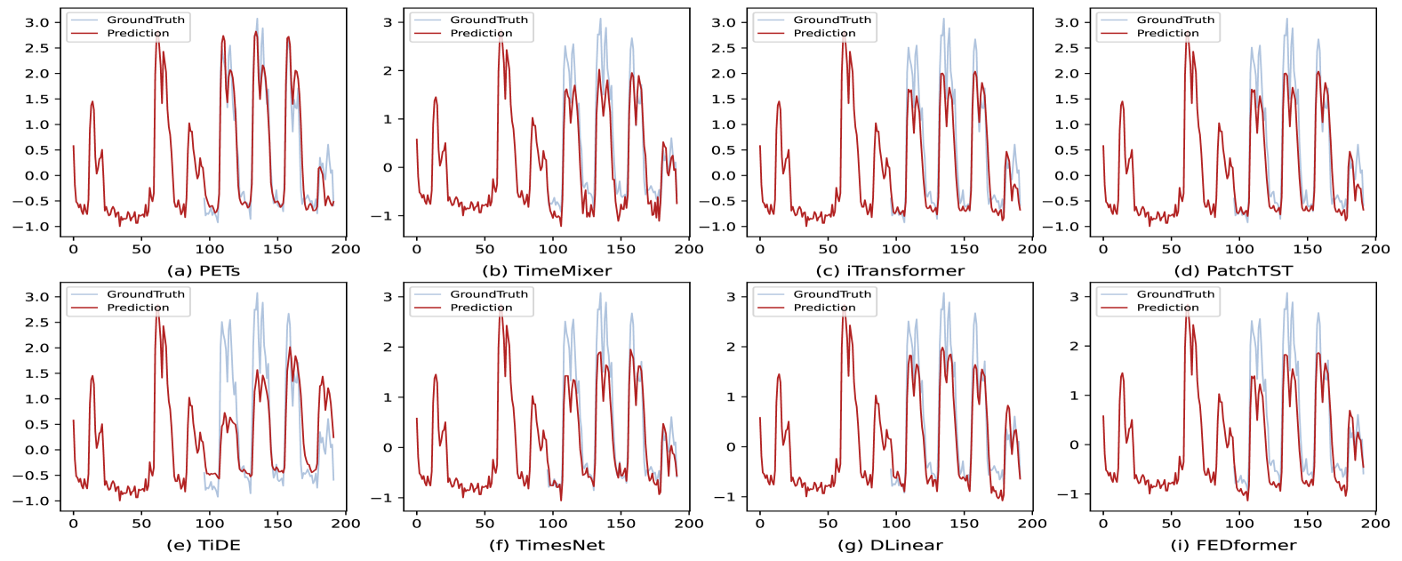
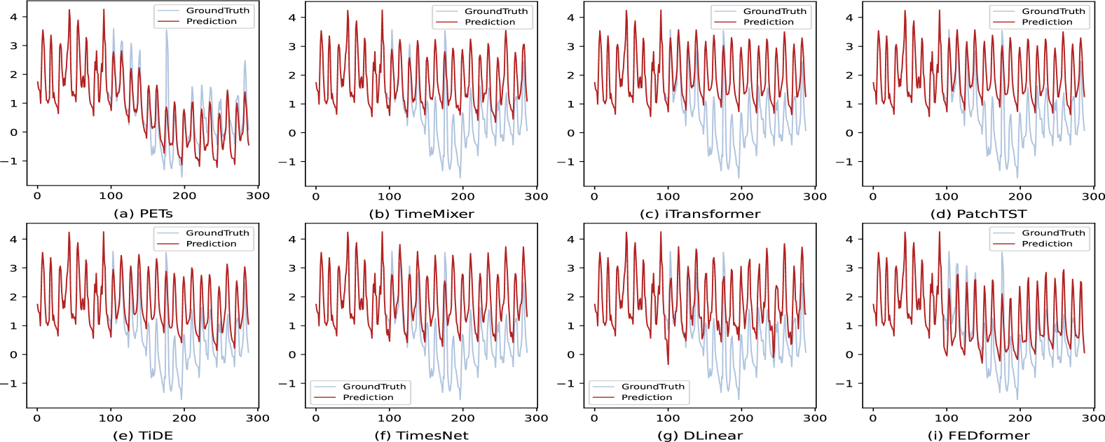
Figure 20: Prediction cases from Electricity by different models under the input-96-predict-96 settings.

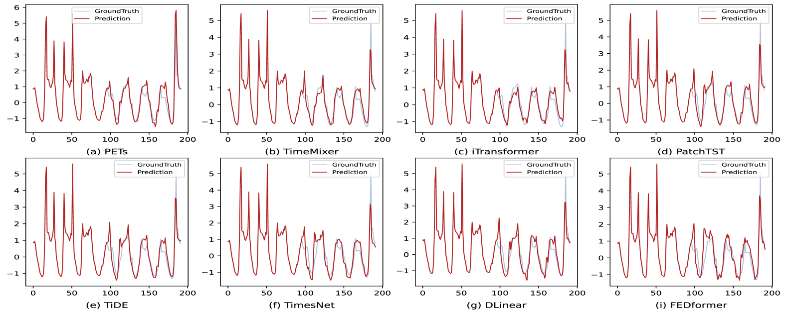
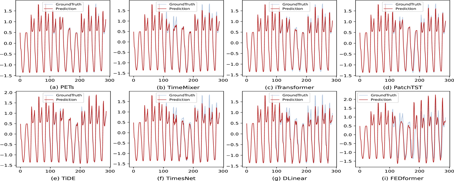
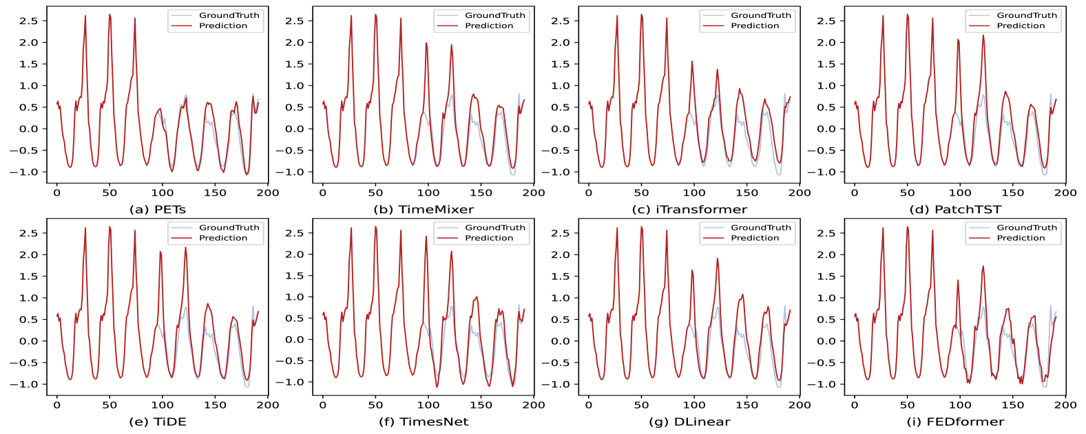
Figure 21: Prediction cases from Traffic by different models under the input-96-predict-96 settings.

References

- Alcaraz and Strodthoff [2022] Juan Miguel Lopez Alcaraz and Nils Strodthoff. Diffusion-based time series imputation and forecasting with structured state space models. ArXiv, abs/2208.09399, 2022.
- Ansari et al. [2024] Abdul Fatir Ansari, Lorenzo Stella, Caner Turkmen, Xiyuan Zhang, Pedro Mercado, Huibin Shen, Oleksandr Shchur, Syama Syndar Rangapuram, Sebastian Pineda Arango, Shubham Kapoor, Jasper Zschiegner, Danielle C. Maddix, Michael W. Mahoney, Kari Torkkola, Andrew Gordon Wilson, Michael Bohlke-Schneider, and Yuyang Wang. Chronos: Learning the language of time series. Transactions on Machine Learning Research, 2024. ISSN 2835-8856. URL https://openreview.net/forum?id=gerNCVqqtR.
- Aseeri [2023] Ahmad O. Aseeri. Effective rnn-based forecasting methodology design for improving short-term power load forecasts: Application to large-scale power-grid time series. J. Comput. Sci., 68:101984, 2023.
- Bagnall et al. [2018] A. Bagnall, Hoang Anh Dau, Jason Lines, Michael Flynn, James Large, Aaron George Bostrom, Paul Southam, and Eamonn J. Keogh. The uea multivariate time series classification archive, 2018. ArXiv, abs/1811.00075, 2018.
- Berndt and Clifford [1994] Donald J. Berndt and James Clifford. Using dynamic time warping to find patterns in time series. In KDD Workshop, 1994.
- Cai et al. [2024] Wanlin Cai, Yuxuan Liang, Xianggen Liu, Jianshuai Feng, and Yuankai Wu. Msgnet: Learning multi-scale inter-series correlations for multivariate time series forecasting. In AAAI, 2024.
- Campos et al. [2023] David Campos, Miao Zhang, B. Yang, Tung Kieu, Chenjuan Guo, and Christian S. Jensen. Lightts: Lightweight time series classification with adaptive ensemble distillation. Proceedings of the ACM on Management of Data, 1:1 – 27, 2023.
- Challu et al. [2022] Cristian Challu, Kin G. Olivares, Boris N. Oreshkin, Federico Garza, Max Mergenthaler-Canseco, and Artur W. Dubrawski. N-hits: Neural hierarchical interpolation for time series forecasting. ArXiv, abs/2201.12886, 2022.
- Chen et al. [2001] Chao Chen, Karl F. Petty, Alexander Skabardonis, Pravin Pratap Varaiya, and Zhanfeng Jia. Freeway performance measurement system: Mining loop detector data. Transportation Research Record, 1748:102–96, 2001.
- Chen and Guestrin [2016] Tianqi Chen and Carlos Guestrin. Xgboost: A scalable tree boosting system. Proceedings of the 22nd ACM SIGKDD International Conference on Knowledge Discovery and Data Mining, 2016.
- Chen et al. [2022] Zhe Chen, Yuchen Duan, Wenhai Wang, Junjun He, Tong Lu, Jifeng Dai, and Yu Qiao. Vision transformer adapter for dense predictions. arXiv preprint arXiv:2205.08534, 2022.
- Chi and Chi [2022] Yeong Nain Chi and Orson Chi. Time series forecasting global price of bananas using hybrid arima-narnn model. Data Science in Finance and Economics, 2022.
- Das et al. [2023] Abhimanyu Das, Weihao Kong, Andrew B. Leach, Shaan Mathur, Rajat Sen, and Rose Yu. Long-term forecasting with tide: Time-series dense encoder. ArXiv, abs/2304.08424, 2023.
- Das et al. [2024] Abhimanyu Das, Weihao Kong, Rajat Sen, and Yichen Zhou. A decoder-only foundation model for time-series forecasting. In Ruslan Salakhutdinov, Zico Kolter, Katherine Heller, Adrian Weller, Nuria Oliver, Jonathan Scarlett, and Felix Berkenkamp, editors, Proceedings of the 41st International Conference on Machine Learning, volume 235 of Proceedings of Machine Learning Research, pages 10148–10167. PMLR, 21–27 Jul 2024.
- Dempster et al. [2019] Angus Dempster, Franccois Petitjean, and Geoffrey I. Webb. Rocket: exceptionally fast and accurate time series classification using random convolutional kernels. Data Mining and Knowledge Discovery, 34:1454–1495, 2019.
- Du et al. [2021] Zhekai Du, Jingjing Li, Hongzu Su, Lei Zhu, and Ke Lu. Cross-domain gradient discrepancy minimization for unsupervised domain adaptation. 2021 IEEE/CVF Conference on Computer Vision and Pattern Recognition (CVPR), pages 3936–3945, 2021.
- Fan et al. [2023] Wei Fan, Pengyang Wang, Dongkun Wang, Dongjie Wang, Yuanchun Zhou, and Yanjie Fu. Dish-ts: A general paradigm for alleviating distribution shift in time series forecasting. In AAAI, 2023.
- Fawaz et al. [2018] Hassan Ismail Fawaz, Germain Forestier, Jonathan Weber, Lhassane Idoumghar, and Pierre-Alain Muller. Deep learning for time series classification: a review. Data Mining and Knowledge Discovery, 33:917–963, 2018.
- Fortuin et al. [2019] Vincent Fortuin, Dmitry Baranchuk, Gunnar Rätsch, and Stephan Mandt. Gp-vae: Deep probabilistic time series imputation. In International Conference on Artificial Intelligence and Statistics, 2019.
- Franceschi et al. [2019] Jean-Yves Franceschi, Aymeric Dieuleveut, and Martin Jaggi. Unsupervised scalable representation learning for multivariate time series. In NeurIPS, 2019.
- Goerg [2013] Georg M. Goerg. Forecastable component analysis. In International Conference on Machine Learning, 2013.
- Goswami et al. [2024] Mononito Goswami, Konrad Szafer, Arjun Choudhry, Yifu Cai, Shuo Li, and Artur Dubrawski. Moment: A family of open time-series foundation models. In ICML, 2024.
- Gruver et al. [2024] Nate Gruver, Marc Finzi, Shikai Qiu, and Andrew G Wilson. Large language models are zero-shot time series forecasters. Advances in Neural Information Processing Systems, 36, 2024.
- Gu et al. [2021] Albert Gu, Karan Goel, and Christopher R’e. Efficiently modeling long sequences with structured state spaces. ArXiv, abs/2111.00396, 2021.
- Gu et al. [2022] Albert Gu, Karan Goel, and Christopher Ré. Efficiently modeling long sequences with structured state spaces. In ICLR, 2022.
- Harutyunyan et al. [2017] Hrayr Harutyunyan, Hrant Khachatrian, David C. Kale, and A. G. Galstyan. Multitask learning and benchmarking with clinical time series data. Scientific Data, 6, 2017.
- Hochreiter and Schmidhuber [1997] S. Hochreiter and J. Schmidhuber. Long short-term memory. Neural Comput., 1997.
- Jin et al. [2023] Ming Jin, Shiyu Wang, Lintao Ma, Zhixuan Chu, James Y. Zhang, Xiao Long Shi, Pin-Yu Chen, Yuxuan Liang, Yuan-Fang Li, Shirui Pan, and Qingsong Wen. Time-llm: Time series forecasting by reprogramming large language models. ArXiv, abs/2310.01728, 2023.
- Kingma and Ba [2014] Diederik P. Kingma and Jimmy Ba. Adam: A method for stochastic optimization. CoRR, abs/1412.6980, 2014.
- Kitaev et al. [2020] Nikita Kitaev, Lukasz Kaiser, and Anselm Levskaya. Reformer: The efficient transformer. In ICLR, 2020.
- Kontopoulou et al. [2023] Vaia I. Kontopoulou, Athanasios D. Panagopoulos, Ioannis Kakkos, and George K. Matsopoulos. A review of arima vs. machine learning approaches for time series forecasting in data driven networks. Future Internet, 15:255, 2023.
- Lai et al. [2017] Guokun Lai, Wei-Cheng Chang, Yiming Yang, and Hanxiao Liu. Modeling long- and short-term temporal patterns with deep neural networks. The 41st International ACM SIGIR Conference on Research & Development in Information Retrieval, 2017.
- Lai et al. [2018] Guokun Lai, Wei-Cheng Chang, Yiming Yang, and Hanxiao Liu. Modeling long-and short-term temporal patterns with deep neural networks. In SIGIR, 2018.
- Lee et al. [2023] Heng Yew Lee, Woan Lin Beh, and Kong Hoong Lem. Forecasting with information extracted from the residuals of arima in financial time series using continuous wavelet transform. Int. J. Bus. Intell. Data Min., 22:70–99, 2023.
- Li et al. [2019] Shiyang Li, Xiaoyong Jin, Yao Xuan, Xiyou Zhou, Wenhu Chen, Yu-Xiang Wang, and Xifeng Yan. Enhancing the locality and breaking the memory bottleneck of transformer on time series forecasting. In NeurIPS, 2019.
- Li et al. [2023a] Zhe Li, Shiyi Qi, Yiduo Li, and Zenglin Xu. Revisiting long-term time series forecasting: An investigation on linear mapping. ArXiv, abs/2305.10721, 2023a.
- Li et al. [2023b] Zhe Li, Zhongwen Rao, Lujia Pan, and Zenglin Xu. Mts-mixers: Multivariate time series forecasting via factorized temporal and channel mixing. ArXiv, abs/2302.04501, 2023b.
- Lin et al. [2024] Shengsheng Lin, Weiwei Lin, Xinyi Hu, Wentai Wu, Ruichao Mo, and Haocheng Zhong. Cyclenet: Enhancing time series forecasting through modeling periodic patterns. In NIPS, 2024.
- Liu and Chen [2023] Jiexi Liu and Songcan Chen. Timesurl: Self-supervised contrastive learning for universal time series representation learning. In AAAI, 2023.
- Liu et al. [2021a] Minhao Liu, Ailing Zeng, Mu-Hwa Chen, Zhijian Xu, Qiuxia Lai, Lingna Ma, and Qiang Xu. Scinet: Time series modeling and forecasting with sample convolution and interaction. In NeurIPS, 2021a.
- Liu et al. [2021b] Shizhan Liu, Hang Yu, Cong Liao, Jianguo Li, Weiyao Lin, Alex X Liu, and Schahram Dustdar. Pyraformer: Low-complexity pyramidal attention for long-range time series modeling and forecasting. In ICLR, 2021b.
- Liu et al. [2022] Yong Liu, Haixu Wu, Jianmin Wang, and Mingsheng Long. Non-stationary transformers: Rethinking the stationarity in time series forecasting. In NeurIPS, 2022.
- Liu et al. [2024] Yong Liu, Tengge Hu, Haoran Zhang, Haixu Wu, Shiyu Wang, Lintao Ma, and Mingsheng Long. itransformer: Inverted transformers are effective for time series forecasting, 2024.
- Luo and Wang [2024] Donghao Luo and Xue Wang. Moderntcn: A modern pure convolution structure for general time series analysis. In ICLR, 2024.
- Makridakis et al. [2018] Spyros Makridakis, Evangelos Spiliotis, and Vassilios Assimakopoulos. The m4 competition: Results, findings, conclusion and way forward. International Journal of Forecasting, 2018.
- Nie et al. [2023] Yuqi Nie, Nam H. Nguyen, Phanwadee Sinthong, and Jayant Kalagnanam. A time series is worth 64 words: Long-term forecasting with transformers. ArXiv, abs/2211.14730, 2023.
- Oreshkin et al. [2019] Boris N. Oreshkin, Dmitri Carpov, Nicolas Chapados, and Yoshua Bengio. N-beats: Neural basis expansion analysis for interpretable time series forecasting. ArXiv, abs/1905.10437, 2019.
- Paszke et al. [2019] Adam Paszke, S. Gross, Francisco Massa, A. Lerer, James Bradbury, Gregory Chanan, and Trevor Killeen. Pytorch: An imperative style, high-performance deep learning library. In NeurIPS, 2019.
- Sezer et al. [2019] Omer Berat Sezer, Mehmet Ugur Gudelek, and Ahmet Murat Ozbayoglu. Financial time series forecasting with deep learning : A systematic literature review: 2005-2019. ArXiv, abs/1911.13288, 2019.
- Shi et al. [2015] Xingjian Shi, Zhourong Chen, Hao Wang, D. Y. Yeung, Wai-Kin Wong, and Wang chun Woo. Convolutional lstm network: A machine learning approach for precipitation nowcasting. In NIPS, 2015.
- Tang et al. [2020] Wensi Tang, Guodong Long, Lu Liu, Tianyi Zhou, Michael Blumenstein, and Jing Jiang. Omni-scale cnns: a simple and effective kernel size configuration for time series classification. In International Conference on Learning Representations, 2020.
- Tashiro et al. [2021] Yusuke Tashiro, Jiaming Song, Yang Song, and Stefano Ermon. Csdi: Conditional score-based diffusion models for probabilistic time series imputation. In NIPS, 2021.
- Thissen et al. [2003] Uwe Thissen, Rob van Brakel, A. P. de Weijer, Willem J. Melssen, and Lutgarde M. C. Buydens. Using support vector machines for time series prediction. Chemometrics and Intelligent Laboratory Systems, 69:35–49, 2003.
- Vaswani et al. [2017] Ashish Vaswani, Noam M. Shazeer, Niki Parmar, Jakob Uszkoreit, Llion Jones, Aidan N. Gomez, Lukasz Kaiser, and Illia Polosukhin. Attention is all you need. In NeurIPS, 2017.
- Wang et al. [2023] Huiqiang Wang, Jian Peng, Feihu Huang, Jince Wang, Junhui Chen, and Yifei Xiao. MICN: Multi-scale local and global context modeling for long-term series forecasting. In ICLR, 2023.
- Wang et al. [2024a] Shiyu Wang, Jiawei Li, Xiao Ming Shi, Zhou Ye, Baichuan Mo, Wenze Lin, Shengtong Ju, Zhixuan Chu, and Ming Jin. Timemixer++: A general time series pattern machine for universal predictive analysis. ArXiv, abs/2410.16032, 2024a.
- Wang et al. [2024b] Shiyu Wang, Haixu Wu, Xiao Long Shi, Tengge Hu, Huakun Luo, Lintao Ma, James Y. Zhang, and Jun Zhou. Timemixer: Decomposable multiscale mixing for time series forecasting. In ICLR, 2024b.
- Wang et al. [2024c] Yihang Wang, Yuying Qiu, Peng Chen, Kai Zhao, Yang Shu, Zhongwen Rao, Lujia Pan, Bin Yang, and Chenjuan Guo. Rose: Register assisted general time series forecasting with decomposed frequency learning. ArXiv, abs/2405.17478, 2024c.
- Wang et al. [2024d] Zexin Wang, Changhua Pei, Minghua Ma, Xin Wang, Zhihan Li, Dan Pei, S. Rajmohan, Dongmei Zhang, Qingwei Lin, Haiming Zhang, Jianhui Li, and Gaogang Xie. Revisiting vae for unsupervised time series anomaly detection: A frequency perspective. Proceedings of the ACM on Web Conference 2024, 2024d.
- Woo et al. [2022] Gerald Woo, Chenghao Liu, Doyen Sahoo, Akshat Kumar, and Steven C. H. Hoi. Etsformer: Exponential smoothing transformers for time-series forecasting. arXiv preprint arXiv:2202.01381, 2022.
- Woo et al. [2024] Gerald Woo, Chenghao Liu, Akshat Kumar, Caiming Xiong, Silvio Savarese, and Doyen Sahoo. Unified training of universal time series forecasting transformers. In ICML, 2024.
- Wu et al. [2021] Haixu Wu, Jiehui Xu, Jianmin Wang, and Mingsheng Long. Autoformer: Decomposition transformers with Auto-Correlation for long-term series forecasting. In NeurIPS, 2021.
- Wu et al. [2022] Haixu Wu, Jialong Wu, Jiehui Xu, Jianmin Wang, and Mingsheng Long. Flowformer: Linearizing transformers with conservation flows. In International Conference on Machine Learning, 2022.
- Wu et al. [2023] Haixu Wu, Tengge Hu, Yong Liu, Hang Zhou, Jianmin Wang, and Mingsheng Long. Timesnet: Temporal 2d-variation modeling for general time series analysis. In ICLR, 2023.
- Xia et al. [2024] Chunlong Xia, Xinliang Wang, Feng Lv, Xin Hao, and Yifeng Shi. Vit-comer: Vision transformer with convolutional multi-scale feature interaction for dense predictions. 2024 IEEE/CVF Conference on Computer Vision and Pattern Recognition (CVPR), pages 5493–5502, 2024.
- Xu et al. [2021] Jiehui Xu, Haixu Wu, Jianmin Wang, and Mingsheng Long. Anomaly transformer: Time series anomaly detection with association discrepancy. In ICLR, 2021.
- Xu et al. [2024] Zhijian Xu, Ailing Zeng, and Qiang Xu. Fits: Modeling time series with 10k parameters. In ICLR, 2024.
- Yi et al. [2023] Kun Yi, Qi Zhang, Wei Fan, Shoujin Wang, Pengyang Wang, Hui He, Ning An, Defu Lian, Longbing Cao, and Zhendong Niu. Frequency-domain MLPs are more effective learners in time series forecasting. In NeurIPS, 2023.
- Yi et al. [2024] Kun Yi, Jingru Fei, Qi Zhang, Hui He, Shufeng Hao, Defu Lian, and Wei Fan. Filternet: Harnessing frequency filters for time series forecasting. In NIPS, 2024.
- Yin et al. [2021] Xueyan Yin, Genze Wu, Jinze Wei, Yanming Shen, Heng Qi, and Baocai Yin. Deep learning on traffic prediction: Methods, analysis, and future directions. IEEE Transactions on Intelligent Transportation Systems, 23:4927–4943, 2021.
- Zeng et al. [2023] Ailing Zeng, Muxi Chen, Lei Zhang, and Qiang Xu. Are transformers effective for time series forecasting? In AAAI, 2023.
- Zhang [2003] Guoqiang Peter Zhang. Time series forecasting using a hybrid arima and neural network model. Neurocomputing, 50:159–175, 2003.
- Zhang et al. [2023] Yitian Zhang, Liheng Ma, Soumyasundar Pal, Yingxue Zhang, and Mark Coates. Multi-resolution time-series transformer for long-term forecasting. In International Conference on Artificial Intelligence and Statistics, 2023.
- Zhao et al. [2020] Hang Zhao, Yujing Wang, Juanyong Duan, Congrui Huang, Defu Cao, Yunhai Tong, Bixiong Xu, Jing Bai, Jie Tong, and Qi Zhang. Multivariate time-series anomaly detection via graph attention network. 2020 IEEE International Conference on Data Mining (ICDM), pages 841–850, 2020.
- Zhou et al. [2021] Haoyi Zhou, Shanghang Zhang, Jieqi Peng, Shuai Zhang, Jianxin Li, Hui Xiong, and Wancai Zhang. Informer: Beyond efficient transformer for long sequence time-series forecasting. In AAAI, 2021.
- Zhou et al. [2022a] Tian Zhou, Ziqing Ma, Qingsong Wen, Xue Wang, Liang Sun, and Rong Jin. FEDformer: Frequency enhanced decomposed transformer for long-term series forecasting. In ICML, 2022a.
- Zhou et al. [2022b] Tian Zhou, Ziqing Ma, xue wang, Qingsong Wen, Liang Sun, Tao Yao, Wotao Yin, and Rong Jin. Film: Frequency improved legendre memory model for long-term time series forecasting. In NeurIPS, 2022b.
- Zhou et al. [2023] Tian Zhou, Peisong Niu, Xue Wang, Liang Sun, and Rong Jin. One fits all: Power general time series analysis by pretrained LM. In NIPS, 2023.