Abstract

Graph neural networks (GNNs) are widely used for learning node embeddings in graphs, typically adopting a message-passing scheme. This approach, however, leads to the neighbor explosion problem, with exponentially growing computational and memory demands as layers increase. Graph sampling has become the predominant method for scaling GNNs to large graphs, mitigating but not fully solving the issue. Pre-propagation GNNs (PP-GNNs) represent a new class of models that decouple feature propagation from training through pre-processing, addressing neighbor explosion in theory. Yet, their practical advantages and system-level optimizations remain underexplored. This paper provides a comprehensive characterization of PP-GNNs, comparing them with graph-sampling-based methods in training efficiency, scalability, and accuracy. While PP-GNNs achieve comparable accuracy, we identify data loading as the key bottleneck for training efficiency and input expansion as a major scalability challenge. To address these issues, we propose optimized data loading schemes and tailored training methods that improve PP-GNN training throughput by an average of 15$\times$ over the PP-GNN baselines, with speedup of up to 2 orders of magnitude compared to sampling-based GNNs on large graph benchmarks. Our implementation is publicly available at https://github.com/cornell-zhang/preprop-gnn.

1 Introduction

Message-passing-based graph neural networks (MP-GNNs) have become a cornerstone for graph representation learning, achieving success in various tasks like node classification Veličković et al. (2018); Wu et al. (2023); Kipf & Welling (2017), link prediction Zhang & Chen (2018); Schütt et al. (2017), and graph clustering Zhang et al. (2019); Ying et al. (2018b); Tsitsulin et al. (2023). However, scaling MP-GNNs to large graphs remains a significant challenge.

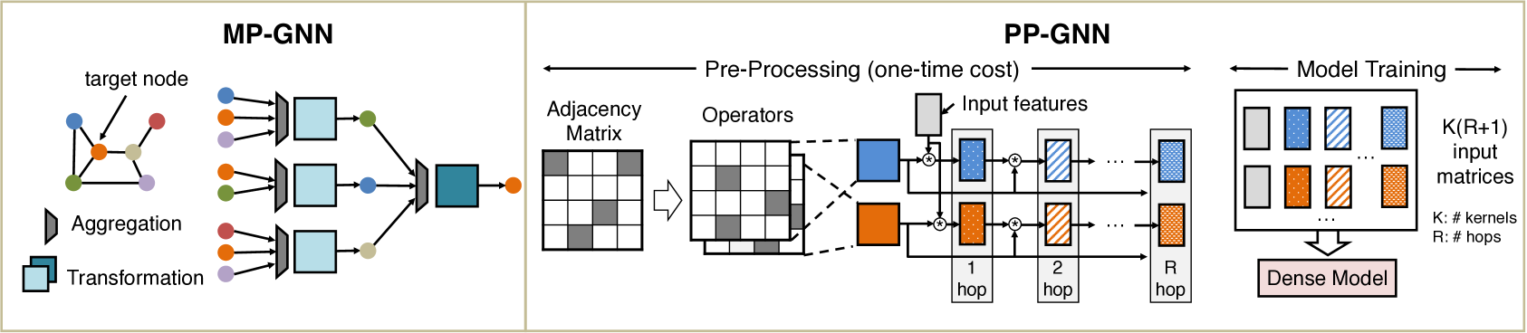
Figure 1: General structure of MP-GNN and PP-GNN models.

The message-passing framework Gilmer et al. (2017) consists of two iterative steps: (1) feature aggregation and (2) transformation. Within this framework, each node collects feature embeddings from its neighbors and then transforms them using a learnable function. We show the architecture of MP-GNN models in Figure 1. The main challenge in scaling MP-GNNs to large graphs stems from the “neighbor explosion” problem Hamilton et al. (2017), where nodes must recursively collect embeddings from increasingly larger neighborhoods across layers, causing the number of embeddings to grow exponentially with each additional layer.

To address this challenge, various prior arts have introduced sampling-based GNNs to reduce the compute and memory footprint during message passing. Those models encompass node-wise sampling to limit neighborhood sizes per node Chen et al. (2017); Hamilton et al. (2017), layer-wise sampling to reduce node counts per layer Chen et al. (2018); Zou et al. (2019), and graph-wise sampling to control overall subgraph size Chiang et al. (2019); Zeng et al. (2020). However, the sampling-based GNNs face several major limitations. First, node-wise sampling methods only partially mitigate the neighbor explosion problem, as their time complexity still increases exponentially with the number of layers. More importantly, the sampling algorithms modify the graph topology by design, which inevitably breaks the functionality of computation graphs such as logic networks Wu et al. (2023) and dataflow graphs Phothilimthana et al. (2024), resulting in accuracy degradation on their downstream tasks Deng et al. (2024).

To circumvent the limitations of MP-GNNs, a new class of models known as pre-propagation GNNs (PP-GNNs) has emerged to tackle the scalability issue from a different angle Wu et al. (2019); Frasca et al. (2020); Dong et al. (2021); Zhang et al. (2022); Liao et al. (2022); Chen et al. (2020b); Deng et al. (2024); Zhu & Koniusz (2020). These models perform feature aggregation in a preprocessing step, eliminating the need for this computationally expensive step during model training. This approach theoretically offers two advantages over MP-GNNs. First, by decoupling nodes from interdependencies introduced by feature aggregation, nodes are processed independently during training, effectively addressing the neighbor explosion problem. Second, previous efforts Huang et al. (2020) have shown that within the message-passing framework, feature aggregation is typically more time-consuming than transformation due to its sparse nature. By restricting training to dense computations, PP-GNNs are expected to achieve greater efficiency. Importantly, the input data preprocessing is a one-time cost that can be amortized across multiple rounds of hyperparameter tuning and model architecture adjustments.

In this work, we conduct the first systematic characterization of PP-GNN models, comparing their training efficiency, scalability, and accuracy with MP-GNN models. We find that although PP-GNNs achieve comparable accuracy as MP-GNNs on commonly used large graph benchmarks, they do not exhibit clear training efficiency advantages over MP-GNNs that leverage tailored system-level optimizations.

During our characterization, we identify two primary challenges for PP-GNN training: data loading as the major efficiency bottleneck and input expansion as the main scalability issue. Data loading, consisting of batch assembly and data transfer, dominates training time due to lightweight computations in PP-GNNs, and the input expansion problem stems from the architecture of PP-GNN models, where the size of input features expands as more hops of neighbors are used, potentially exceeding host memory capacity.

To address these challenges, we propose several system-level optimizations. First, we introduce a customized data loader with an efficient batch assembly operation to reduce host-side data preparation overhead. Second, we design a double-buffer-based data prefetching scheme to decouple data loading from GPU-side computation. These optimizations significantly reduce data loading overhead while adhering to the standard training method, stochastic gradient descent with random reshuffling (SGD-RR) Mishchenko et al. (2020). Additionally, we propose chunk reshuffling, which shuffles training data at a coarser granularity, enabling bulk data transfer and more efficient GPU-side batch assembly. Moreover, we leverage chunk reshuffling to extend our training pipeline to leverage GPU direct storage (GDS) Thompson & Newburn (2019) access, efficiently handling input sizes exceeding host memory capacity.

We further integrate these optimizations into an automated training configuration system for PP-GNNs, which detects hardware configurations and determines the best data placement and training strategies. With these system optimizations, PP-GNNs demonstrate significantly higher training efficiency on various commonly used large graph benchmarks, including those with up to 100 million nodes.

Our main contributions are as follows:

• We present the first comprehensive study comparing both the training efficiency and accuracy of PP-GNNs and MP-GNNs on commonly-used large graph benchmarks.

• We identify data loading as the critical efficiency bottleneck and the input expansion problem as the major scalability challenge for PP-GNN training.

• We propose various system-level optimizations to tackle the two challenges, including efficient batch assembly schemes, double-buffer-based data prefetching, and a tailored chunk reshuffling training method. Additionally, we propose an automated training configuration system for PP-GNNs that accommodates various graph sizes based on hardware configurations and a data placement policy.

• Our optimizations improve PP-GNN training efficiency on average 15$\times$ compared to vanilla PP-GNN implementations and show comparable training efficiency when fetching input data directly from the solid-state drives (SSD) compared to from the host memory. After optimization, compared to MP-GNN models with state-of-the-art graph samplers, our optimized PP-GNNs achieve on average 9.9$\times$ and up to 2 orders of magnitude higher training throughput with higher accuracy on large graphs.

2 Preliminaries

This section introduces the key concepts related to GNNs, including the message-passing paradigm, graph sampling algorithms, and PP-GNNs. We also introduce existing MP-GNN training systems in this section.

2.1 Notations

In the following sections, we define a graph as $G=(V,E)$, where $V$ is the node set and $E$ is the edge set. We define $|V|=n$ as the total number of nodes in the graph and $|E|=m$ as the total number of edges. Each node $v\in V$ has a neighborhood set $N(v)$. Let $A\in\mathbb{R}^{n\times n}$ represent the adjacency matrix and $D\in\mathbb{R}^{n\times n}$ represent the diagonal degree matrix. $X\in\mathbb{R}^{n\times F}$ denotes the input node feature matrix with $F$ as the input feature dimension.

2.2 General Structure of MP-GNNs

In general, GNN models take in graph-related information, such as the graph topology and node features, to learn latent node embeddings. Most popular GNN models can be generalized within the message-passing-based framework Gilmer et al. (2017), which is articulated in Eq. (1). Here, $h_{v}^{(k)}$ denotes the embedding of node $v$ in layer $k$, with $h_{v}^{(0)}=x_{v}$. $l_{k}$ represents a transformation function, $f_{k}$ an aggregation function, and $e_{vu}$ the edge attribute between nodes $v$ and $u$.

$$h_{v}^{(k)}=l_{k}\left(h_{v}^{(k-1)},f_{k}\left(\{(h_{u}^{(k-1)},e_{vu})\mid\forall u\in N(v)\}\right)\right)$$ (1)

Message passing occurs within the aggregation function $f_{k}$, where node $v$ aggregates embeddings from its one-hop neighbors, a process also known as feature propagation. As indicated in Equation (1), the aggregation function is applied recursively across layers, which can lead to the neighbor explosion problem. Various GNN models are specific instances of this generalized framework. For example, GraphSAGE Hamilton et al. (2017) employs mean, Long Short-Term Memory (LSTM), or pooling aggregators in its aggregation function. The Graph Attention Network (GAT) Veličković et al. (2018) incorporates a learnable attention mechanism to assign different weights to neighbors during feature propagation. Both models employ a Multi-Layer Perceptron (MLP) as the transformation function.

2.3 Graph Sampling

Graph sampling is a widely adopted technique to scale MP-GNNs on large graphs, categorized into three types: node-wise sampling Chen et al. (2017); Hamilton et al. (2017); Balin & Çatalyürek (2024), layer-wise sampling Chen et al. (2018); Zou et al. (2019), and graph-wise sampling Chiang et al. (2019); Zeng et al. (2020). Node-wise samplers, such as the one introduced in GraphSAGE Hamilton et al. (2017), limit neighborhood size during sampling but still face the neighbor explosion problem, with node count growing exponentially by layer. Layer-wise sampling methods sample a fixed number of nodes per layer, resulting in linear growth but struggling with sparse connectivity. LADIES Zou et al. (2019) tackles this problem with layer-dependent sampling for better connectivity. Graph-wise sampling methods, such as GraphSAINT Zeng et al. (2020), sample subgraphs with a fixed number of nodes or edges, maintaining a subgraph size independent of model depth while ensuring connection. LABOR Balin & Çatalyürek (2024) is a State-of-The-Art (SoTA) hybrid sampler combining the strength of both node-wise and layer-wise sampling, leading to fewer nodes sampled compared to node-wise samplers while maintaining an adaptive nature to different graph sizes.

2.4 GNN Training Systems

In sampling-based GNN training, the primary bottleneck is the graph sampling process, which includes node sampling and feature extraction Liu et al. (2023); Yang et al. (2022); Lin et al. (2020). Various training systems have been developed to optimize this process by leveraging GPUs. For instance, DGL Wang (2019) accelerates node sampling and feature extraction on GPUs, provided the graph data fits entirely into GPU memory. PaGraph Lin et al. (2020) utilizes GPU-based caching of node features while relying on CPU for node sampling. GNNLab Yang et al. (2022) employs GPUs for both node sampling and feature caching. These techniques can enhance MP-GNN training efficiency in both single-GPU and multi-GPU environments. Additional strategies employed in these systems include the use of NVLinks between GPUs to minimize communication overhead Cai et al. (2023), hardware-aware graph partitioning Sun et al. (2023); Tan et al. (2023), and GPU kernel optimizaitons Huang et al. (2024); Wang (2019).

2.5 Pre-propgation GNNs

PP-GNNs Frasca et al. (2020); Deng et al. (2024); Zhang et al. (2022); Chen et al. (2020b); Liao et al. (2024; 2022); Yu et al. (2020); Wu et al. (2019) have recently emerged as a promising approach to scaling GNN training. We show the general structure of PP-GNN models in Figure 1. During preprocessing, node features are aggregated in a manner similar to feature propagation in MP-GNNs, but instead of relying directly on the adjacency matrix, operators derived from the adjacency matrix are typically employed. From a spectral perspective, these operators act as graph signal filters applied to the input graph Gasteiger et al. (2019). Given that most MP-GNNs effectively perform low-pass filtering on the input graph signal Nt & Maehara (2019), PP-GNNs can achieve comparable accuracy by learning on already filtered graph data. Like MP-GNNs, node features are propagated by multiplying the operators with the node feature matrix, yielding features at different hops through successive multiplications. The resulting node features are then stored and reused in the training phase, where a dense model is typically employed to learn node representations.

PP-GNN models can be generalized as follows:

$$\text{Preprocess: }S_{k} =\{\mathbf{X},\mathbf{B}_{k}\mathbf{X},\ldots,\mathbf{B}_{k}^{R}\mathbf{X}\},\quad k=1,\ldots,K$$ (2)

$$\text{Train: }H =l(S_{1},\ldots,S_{K}),\quad\quad Y=o(H)$$ (3)

In Eq. (2), X denotes the input feature matrix, R represents the number of hops, and $\mathbf{B}_{k}$ for $k=1,\ldots,K$ are $K$ operators. After preprocessing, we get $K$ sets of node features, denoted as $S_{k}$, each of which consists of $R+1$ matrices, corresponding to features that incorporate information from up to $R$-hop neighbors, along with the original node features. In Eq. (3), $l(\cdot)$ represents a specific learnable transformation function applied on all sets of $\mathbf{S}$, which outputs a single node embedding matrix $H$. An output function $o(\cdot)$ then transforms $H$ to the desired output shape.

For SGC Wu et al. (2019), the operator is the normalized adjacency matrix expressed as $\mathbf{B}=\tilde{\mathbf{D}}^{-\frac{1}{2}}\tilde{\mathbf{A}}\tilde{\mathbf{D}}^{-\frac{1}{2}}$, where $\tilde{A}=I+A$ is the adjacency matrix with self-loops, and $\tilde{D}$ is the corresponding diagonal degree matrix. $o(\cdot)$ is a linear transformation while $l(\cdot)$ can be simplified as $\delta_{ir}=1\text{ if }i=r\text{ otherwise }0$. For SIGN Frasca et al. (2020), the operator can be the normalized adjacency matrix or those derived from Personalized PageRank (PPR) or Heat kernel Gasteiger et al. (2019). The transformation function $l(\cdot)$ first concatenates matrices belonging to the same hop from different operators and then learns $R+1$ weight matrices for each hop. The output function $o(\cdot)$ is an MLP. For HOGA Deng et al. (2024), the operator is captured by the normalized adjacency matrix. The transformation function adopts a transformer-like mechanism, which treats the $R+1$ input feature vectors of each node as $R+1$ tokens. An MLP is employed as the output function.

3 PP-GNN Characterization

As an emerging family of GNN models, PP-GNNs have yet to benefit from tailored system-level optimizations, raising questions about their practical training efficiency and scalability compared to MP-GNNs. Their model expressivity on commonly-used graph datasets has not been thoroughly explored either. In this section, we present a systematic characterization of PP-GNNs, examining their theoretical complexity, accuracy, training efficiency, and scalability.

3.1 Complexity Analysis

First, we compare the theoretical computational cost and memory complexity of training PP-GNNs and MP-GNNs, as listed in Table LABEL:table:complexity_concise. In this table, we do not consider the sampling process for MP-GNNs. Here $b$ represents the mini-batch size, and we assume the number of nodes sampled per layer in LADIES and per subgraph in GraphSAINT is the same as $b$; $C$ represents the neighborhood size per node after sampling in GraphSAGE and LABOR, which is usually much smaller than $b$. To simplify the analysis, we assume the same dimension for the input layer and hidden layers, using $F$ to denote both. Other notations used in the complexity analysis are defined in Section 2.1.

There are two major components in the computational cost for MP-GNNs, one arising from feature propagation, denoted in red, and the other from feature transformation, denoted in blue. Prior studies Huang et al. (2020) suggest that the former usually takes longer in practice due to its sparse nature. According to the table, PP-GNNs are expected to significantly boost the training efficiency, as they eliminate feature propagation from the training process.

3.2 Accuracy

Conventional wisdom suggests that more scalable graph learning approaches like PP-GNNs may compromise accuracy for improved scalability. However, the learning capabilities of PP-GNNs are still not well understood and remain an active area of research Chen et al. (2020a). Meanwhile, work from Deng et al. Deng et al. (2024) shows that PP-GNNs outperform MP-GNNs on several electronic design automation tasks that require complete neighbor information to infer functionality correctly. To this end, we investigate the model accuracy of various approaches on widely used large graph datasets, with detailed information in Table LABEL:tab:datasets.

Our evaluation indicates that, among sampling methods, the LABOR sampler achieves the highest test accuracy across most settings, while HOGA outperforms other PP-GNN models in the majority of cases. Figure LABEL:fig:accuracy illustrates the test accuracy of GraphSAGE Hamilton et al. (2017) employing two different samplers—LABOR Balin & Çatalyürek (2024) and GraphSAINT Zeng et al. (2020)—as well as a PP-GNN model, HOGA, across varying numbers of layers or hops on three datasets. Complete results and hyperparameter settings are provided in Appendix A and D. From Figure LABEL:fig:accuracy we observe two trends: (1) PP-GNNs demonstrate accuracy comparable to MP-GNNs, with LABOR serving as a representative; (2) Expanding the node receptive field tends to improve test accuracy on large graphs—unlike prior arts evaluated on small graphs, using 5/6 layers (hops) further improve accuracy in our experiments, which is consistent with the trend seen in Chiang et al. (2019).

3.3 Practial Training Efficiency

To evaluate the practical training efficiency, we compare MP-GNNs and PP-GNNs from two perspectives: convergence rate and epoch time.

Convergence Rate Comparison. The convergence rate significantly impacts the end-to-end training time of a GNN model. Since different models reach different peak accuracies even on the same dataset, to make a fair comparison, we measure the convergence point as the epoch where each model first reaches 99% of its peak validation accuracy. Figure LABEL:fig:convergence shows the convergence points of different MP-GNNs and PP-GNNs with hyperparameters tuned for optimal accuracy, detailed in Appendix A. Complete results are provided in Appendix B. Our results show that PP-GNNs have on par or faster convergence rate than MP-GNNs.

Epoch Time Comparison. For PP-GNNs, we implemented SIGN Frasca et al. (2020), HOGA Deng et al. (2024), and SGC Wu et al. (2019) in PyTorch, which use the PyTorch data loader to decouple data preparation from model training. For comparison, we also implemented MP-GNN models with various graph sampling algorithms in DGL Wang (2019), adhering to the structures described in their original papers Ying et al. (2018a); Veličković et al. (2018); Zou et al. (2019); Balin & Çatalyürek (2024); Zeng et al. (2020). Detailed settings are provided in Appendix A. With DGL version 0.8 and later, the graph sampling process can be GPU-accelerated. When input data is pinned in host memory, DGL utilizes NVIDIA’s UVA Schroeder (2011) technology, allowing GPU to access data on the host memory with zero-copy. Preloading the input data to GPU memory further reduces end-to-end training time due to the high memory bandwidth available on GPU.

Figure LABEL:fig:training_time_nonopt compares the epoch times among 3-layer MP-GNNs (GraphSAGE with the LABOR sampler) and 3-hop PP-GNNs (SIGN, HOGA, and SGC). The epoch time for GraphSAGE is measured with a vanilla DGL implementation with CPU-based graph sampling and two optimized versions, denoted as SAGE-UVA and SAGE-Preload, representing GPU-based graph sampling with the use of UVA and input preloading, respectively. From Figure LABEL:fig:training_time_nonopt we see system-level optimizations significantly improve MP-GNN training throughput. Consequently, despite theoretical advantages in computational cost (Table LABEL:table:complexity_concise), vanilla PP-GNN implementations take longer epoch time than MP-GNNs fully optimized in DGL.

Further investigation reveals that the primary overhead in the baseline implementation stems from data loading. Figure LABEL:fig:training_time_decomp shows the epoch time breakdown of three PP-GNN models on the ogbn-products dataset, averaged across various hops. The figure highlights that computation is relatively lightweight for PP-GNNs, which is represented as the forward pass, backpropagation, and optimizer step in the figure. In contrast, the epoch time is dominated by data loading. Therefore, system-level optimizations that improve data loading efficiency are crucial for PP-GNNs to achieve their potential training efficiency advantages.

3.4 The Challenge of Input Expansion

Through our characterization, we identify a largely overlooked issue in prior studies of PP-GNNs, which we term the “input expansion problem.” From Eq. (3) we observe that $K(R+1)$ input matrices are generated during preprocessing, each representing an input feature matrix with $i\in R$ hop neighbor information from one of $K$ operators. Consequently, the input feature size is expanded to $K(R+1)$ times larger, as illustrated in Figure 1 (d). For instance, the igb-large dataset Khatua et al. (2023) takes 400 GB for the input features. With a small $R$ and $K$, like $R=3$ and $K=1$, the input data for PP-GNNs will expand to 1.6 TB, exceeding the typical host memory capacity. Consequently, randomly fetching features from the storage system during training will result in severe training efficiency degradation due to low storage random read speed. Therefore, we need system-level solutions to overcome the input expansion problem of PP-GNNs on large graphs.

3.5 Pre-processing Overhead

Compared to MP-GNNs, PP-GNNs require an additional preprocessing step. However, this preprocessing can be considered a one-time cost, as the processed data is stored and reused throughout the training process. Table LABEL:tab:datasets presents the preprocessing time for the datasets used in our evaluation. Typically, training a GNN model involves hundreds of epochs per run, and hyper-parameter tuning may require tens or even hundreds of such runs. As shown in Table LABEL:tab:datasets, the preprocessing overhead is usually much smaller than the time required for a single training run, and thus, can be efficiently amortized over the entire training phase.

4 System Optimizations

Our characterization reveals that data loading time significantly dominates the training time of PP-GNNs. Typically, data loading consists of two steps: batch assembly and data transfer. During batch assembly, the data loader extracts node vectors belonging to the current batch, and transfers them to GPU in the following data transfer step. To reduce the data loading overhead, a straightforward solution involves loading input data into GPU memory to leverage its high bandwidth. However, the input expansion problem limits the feasibility of this approach, as GPU memory typically has a much lower capacity compared to host memory.

To reduce the data loading overhead while maintaining the input data in host memory, we propose several strategies. First, we devise a custom data loader with efficient data indexing to reduce the kernel launching overhead during batch assembly (Section 4.1). Second, we introduce a double-buffer-based data prefetching mechanism on GPU, which largely hides data loading time by pipelining it with computation (Section 4.1). Last, we develop a chunk reshuffling method that allows us to reorder batch assembly and data transfer, enabling GPU-side batch assembly, taking advantage of high GPU memory bandwidth (Section 4.2). Moreover, chunk reshuffling paves the way for scaling to large graphs. By replacing host memory access with GPU direct storage access, we can easily handle input sizes exceeding the host memory capacity (Section 4.3).

4.1 Customized Data Loading

Upon profiling the PP-GNN baseline implementations, we observe that the PyTorch data loader extracts node features individually during batch assembly, resulting in frequent kernel invocations on the host side. As a result, batch assembly dominates the total training time, as depicted in Figure LABEL:fig:system_op_overall (a). To mitigate the redundant kernel launching, we design a customized data loader utilizing the index operator provided by PyTorch to copy the scattered node features into a pinned tensor in host memory, which is then transferred to the GPU asynchronously. This approach is feasible due to the simplicity of the input data format, as PP-GNN inputs are purely dense tensors. By launching the index operator only once per batch, we significantly reduce the kernel launching overhead, as illustrated in Figure LABEL:fig:system_op_overall (b).

Despite this improvement, batch assembly on the host side still incurs significant time, potentially exceeding GPU computation time. This is primarily due to the extraction of scattered data in memory, limited by the host memory bandwidth. A potential solution is to cache node features on GPU to leverage its high memory bandwidth, as adopted by many MP-GNN systems Yang et al. (2022); Sun et al. (2023). However, this approach is unsuitable for PP-GNNs, as the training data lacks both temporal and spatial locality, being accessed only once in a random order every epoch. Instead, we implement a data prefetching scheme using double buffers on GPU, as shown in Figure LABEL:fig:system_op_overall (c). This approach decouples data loading from GPU-side computation, enabling pipelining of these two steps. To achieve this, we use separate threads on the host side for launching compute kernels and data-loading-related kernels. On the GPU side, different streams are utilized for data prefetching and computation. As shown in Figure LABEL:fig:system_op_overall (c), our prefetching scheme effectively hides the batch assembly overhead.

4.2 Chunk Reshuffling

While double-buffer-based prefetching pipelines data loading with computation, it fails to fully eliminate overhead when data loading time exceeds computation time. This overhead arises from (1) batch assembly, constrained by host memory bandwidth, and (2) data transfer, limited by the host-to-GPU interconnect. Since data transfer is already optimized by Direct Memory Access (DMA) technique, further reducing its duration is challenging.

To reduce batch assembly time, we propose a chunk reshuffling training method. In this method, at the start of each epoch, we reshuffle training data indices at the chunk level, with each chunk comprising contiguous node features. Then, we transfer individual chunks belonging to the current batch from host memory to GPU and assemble chunks into batches. This approach takes advantage of the significantly higher DRAM bandwidth on GPU for batch assembly. Although data transfer overhead increases as more DMA transfer kernels are launched, this is minor provided the chunk size is sufficiently large. The efficacy of this approach is illustrated in Figure LABEL:fig:system_op_overall (d). Lastly, chunk reshuffling can be considered a form of insufficient shuffling scheme Meng et al. (2019); Nguyen et al. (2022), which is commonly used in practice. In Section 6.2, our empirical results show that chunk reshuffling has negligible impacts on test accuracy and convergence rate for PP-GNNs.

4.3 Direct Storage Access

The input expansion problem can cause the preprocessed input data of large graphs to exceed the host memory capacity. A naïve implementation fetching individual node features from storage to the host would suffer from slow random reads, resulting in significant data loading overhead.

Our chunk reshuffling method provides a foundation for extending to storage-based training; reading chunks from the storage system is significantly more efficient compared to reading individual node features. By replacing host-memory-reading operators with GPU direct storage access, we retain the benefits of pipelined data loading and computation with our double-buffer-based data prefetching scheme. In our implementation, we leverage the NVIDIA GDS technique Thompson & Newburn (2019) for direct storage access, which automatically utilizes DMA engines and system buffers, ensuring efficient data transfers under various system configurations. To maximize the parallel processing capabilities of modern storage systems and bus bandwidth utilization, we split input features of different hops into separate files, enabling parallel storage access requests.

5 Automated Training Configuration

Building on our system-level optimizations, we extend our training pipeline to develop an automated configuration system tailored for PP-GNNs. This system automates key configurations, particularly for data placement and training methods, optimizing PP-GNN training based on hardware resources and model characteristics. Implemented in PyTorch, our system offers a user-friendly interface, allowing integration of PP-GNN models without model-specific system tweaking. Before training starts, our system assesses the available hardware resources, including the number of GPUs and GPU and host memory capacities. To determine the minimum GPU memory space requirement for a specific model, we adopt an approach similar to PaGraph Lin et al. (2020), where we conduct a one-time training session using storage-based data loading to measure peak GPU memory usage. Combining the information of input data size, our configuration system automatically decides data placement and corresponding training method, as detailed below.

GPU memory. Preloading input data to GPU memory is prioritized due to its high bandwidth. For large datasets, our system supports distributing data across multiple GPUs, with the data loader fetching data in a locality-aware manner Yang & Cong (2019) to adapt to SGD-RR. When data is preloaded to GPU memory, our double-buffer-based prefetching further enhances training efficiency. However, with the high bandwidth of GPU memory, batch assembly is not a bottleneck, making chunk reshuffling negligible for performance. Thus, SGD-RR is preferred in this scenario.

Host Memory. When the input data exceeds GPU memory capacity, it is placed in host memory. With chunk reshuffling, the entire input data must be pinned in host memory for non-blocking transfers. Otherwise, only a buffer proportional to the mini-batch size is pinned. The configure system defaults to SGD-RR for large data to avoid excessive host memory pinning, unless specified by users.

Storage. When the input data exceeds the host memory capacity, our system allows the GPU to fetch data directly from the storage via NVIDIA GDS Thompson & Newburn (2019). Currently, we only support chunk reshuffling in this scenario, since SGD-RR requires fine-grained data access, significantly increasing data loading overhead.

The influence of data placement on training throughput is evaluated in Appendix H.

6 Evaluation

Experiment Setup. We conduct the experiments on a Linux server with two 3.0 GHz Intel Xeon CPUs, 380 GB RAM and four RTX A6000 GPUs. Detailed hardware and software configurations are provided in Appendix C.

Datasets. We use three medium-sized graphs, ogbn-products, pokec, and wiki, each with approximately 2 million nodes for a detailed investigation of the accuracy-efficiency trade-off between PP-GNNs and MP-GNNs. While we classify these as medium-sized, it’s important to note that these graphs are usually considered large graphs in the GNN community Chiang et al. (2019). We use three large graphs, ognb-papers100M, IGB-meduim, and IGB-large to investigate the scalability of PP-GNNs under different scenarios. The datasets are chosen from real-world benchmarks including Open Graph Benchmark (OGB) Hu et al. (2020), Illinois Graph Benchmark (IGB) Khatua et al. (2023), and the Cornell non-homophilous benchmark Lim et al. (2021). The dataset attributes are listed in table LABEL:tab:datasets. Our paper focuses on node classification tasks, which serve as the foundation for link and graph classification.

MP-GNN. We use GraphSAGE Hamilton et al. (2017) and GAT Veličković et al. (2018) as backbone models. We employ the samplers from GraphSAGE Hamilton et al. (2017), LABOR Balin & Çatalyürek (2024), LADIES Zou et al. (2019) and GraphSAINT Zeng et al. (2020) and refer to them as Neighbor, LABOR, LADIES, and SAINT in the following sections, respectively. GraphSAGE is set with a hidden dimension of 256, using the mean aggregator, and GAT is set with a hidden dimension of 128 per channel across 4 channels. We adopt two commonly used 3-layer fanout settings: [15 10 5] for GraphSAEG and [10 10 10] for GAT. This configuration pushes GAT towards accuracy and GraphSAGE towards efficiency, in line with the model complexity and hidden dimension setting, and offers a balanced view of the accuracy-efficiency trade-off of MP-GNN models. Detailed hyperparameter settings are provided in Appendix A.

PP-GNN. We choose SGC Wu et al. (2019), SIGN Frasca et al. (2020), and HOGA Deng et al. (2024) as our PP-GNN models. SGC represents the simplest form of PP-GNNs, consisting of only one linear layer and using only one input matrix. HOGA, which adopts a transformer-like multi-head attention scheme, is a relatively complex PP-GNN model with higher expressivity, while SIGN lies in between. For these PP-GNNs, we use a single operator: the normalized adjacency matrix. For SIGN, we use 3 layers with a hidden dimension of 512. For HOGA, we use a hidden dimension of 256 for medium-sized graphs and 1024 for large graphs, with a single multi-head attention layer. This configuration pushes HOGA towards accuracy and SIGN towards efficiency. Detailed hyperparameter settings are provided in Appendix A.

Baselines. Our PP-GNN baselines are implemented in PyTorch, leveraging PyTorch DataLoader for data loading. The pin_memory attribute is enabled in DataLoader and 2 workers are used to achieve optimal performance. For MP-GNNs, we implement them in DGL Wang (2019), GNNLab Yang et al. (2022), SALIENT++ Kaler et al. (2023) and Ginex Park et al. (2022).

6.1 Accuracy-Efficiency Comparison

This section compares the accuracy and training efficiency of PP-GNNs and MP-GNNs after applying our proposed system-level optimizations. Figure LABEL:fig:Paretowiki shows the accuracy-efficiency trade-offs of PP-GNNs and MP-GNNs on the wiki dataset, with the Pareto frontier indicated in the upper right direction. Diagrams for the ogbn-products and pokec datasets are shown in Appendix D (Figure LABEL:fig:pareto_frontier_products_pokec). Hyperparameter settings are detailed in Appendix A. The primary variable in these experiments is the node receptive field, defined as the number of layers in MP-GNNs and the number of hops in PP-GNNs. All experiments are conducted on a single GPU with data preloaded into GPU memory. GNNLab’s GPU-side input caching does not outperform DGL preloading, and we present only DGL results.

Figure LABEL:fig:Paretowiki and Figure LABEL:fig:pareto_frontier_products_pokec demonstrate that our optimizations push the PP-GNNs to the Pareto frontier on all three datasets. It also shows that HOGA and SIGN achieve comparable accuracy to MP-GNNs with node-wise samplers, with significantly higher training efficiency. SGC, while fastest among all approaches, sacrifices substantial accuracy due to not fully utilizing all the hops. Among all the graph sampling approaches, the SoTA LABOR sampler achieves the Pareto-optimum but still suffers from the neighbor explosion problem to some extent. LADIES and SAINT overcome this problem with a significant sacrifice in test accuracy, occupying the lower parts in the figures.

An important trend observed is that a larger node receptive field enhances model accuracy (a pattern true for both MP-GNNs and PP-GNNs, though the accuracy gains are more pronounced in MP-GNNs). Given that the training time of PP-GNNs increases sub-linearly with additional hops, these models become increasingly competitive in terms of training efficiency as the node receptive field expands. For example, on wiki, SIGN is 9 times faster than SAGE-LABOR with 2 layers or hops, and this advantage grows to 28 times with 6 layers or hops. Moreover, we employ a smaller hidden dimension setting, 128, across models besides their original settings. Reducing the hidden dimension to 128, MP-GNNs experience up to 4% accuracy loss, while HOGA and SIGN only see a 0.5% variation. With a smaller hidden dimension of 128, SIGN is 136$\times$ faster than GAT with a hidden dimension of 512 with 5 hops or layers, while maintaining an accuracy advantage of 3.9% on the test set.

6.2 Influence of Chunk Reshuffling

In this section, we investigate the impact of our proposed chunk reshuffling training method on model accuracy and convergence rate using the three medium-sized graphs. For PP-GNN models, we fix all the hyperparameters except the chunk size, which is selected from 1, 1000, 2000, 4000, 8000. Figure LABEL:fig:SGDCR_HOGA shows the validation accuracy of HOGA with 4 hops. From the figure, we observe that for ogbn-products, the variation in the training curves across different chunk sizes is negligible, with mean test accuracy varying by less than 0.1%. For pokec and wiki, although there are some fluctuations in the training curves, the final test accuracy difference is less than 0.5%. This trend is consistent across other PP-GNN models and hop settings, with complete results in Appendix E. Consequently, in the following sections, we use a chunk size of 8000, equal to the batch size, when employing the chunk reshuffling training method.

6.3 Ablation Study

In this section, we evaluate the efficacy of our techniques for improving data loading efficiency: efficient host-side batch assembly, GPU-side double-buffer-based prefetching, and chunk reshuffling with GPU-based data assembly. Figure LABEL:fig:ablation presents the normalized epoch time of various PP-GNN models across different datasets, with data averaged over 2 to 6 hops and 100 epochs using the geometric mean.

Our results show that efficient host-side batch assembly provides a 3.3$\times$ speedup over the baseline implementation. Adding double-buffer-based prefetching yields an additional 1.9$\times$ speedup. Further, chunk reshuffling with GPU-based batch assembly delivers an additional 2.4$\times$ speedup, resulting in a total 15$\times$ improvement over the baseline. More detailed analysis can be referred to Appendix F.

6.4 Results on Large Graphs

We examine the training efficiency and scalability of different methods on three large graph datasets using GraphSAGE as the MP-GNN model, while HOGA and SIGN as the PP-GNN models. In DGL, we adopt the LABOR sampler, while in GNNLab, SALIENT++, and Ginex, we use their hardcoded neighbor samplers respectively. Inference of GNNLab relies on an older version of DGL which CUDA12.1 does not support, hence we do not report the test accuracy of GNNLab.

First, the ogbn-papers100M graph dataset features instances where labeled nodes constitute only a minor portion of the total node count. For PP-GNNs, the input data size after preprocessing is proportional to the number of labeled nodes, while the information of unlabeled nodes is incorporated during preprocessing. Notably, the original input features for ogbn-papers100M occupy 53 GB, but the labeled part only takes 0.8 GB per hop after preprocessing, fitting comfortably into GPU memory. Conversely, MP-GNNs require accessing the entire graph topology and all input features during training, totaling 77 GB, which exceeds a single GPU’s capacity, making loading all input data into GPU memory infeasible. For MP-GNNs, we use DGL-UVA, SALIENT++, and GNNlab to evaluate their training efficiency on the ogbn-papers100M dataset.

Table LABEL:tab:papers100M shows training throughput and test accuracy under 100 epochs for different approaches with 2 to 4 hops or layers. HOGA achieves the highest accuracy among all methods, with up to 1.76% higher accuracy than SAGE. DGL achieves higher accuracy than SALIENT++ due to the adoption of the LABOR sampler. In terms of training efficiency, SIGN and HOGA achieve up to 5$\times$ and 41$\times$ higher throughput than GraphSAGE on a single GPU. Compared to DGL-UVA, GNNLab improves training efficiency by caching input features and graph topology on GPU, but its hardcoded graph sampler produces larger subgraphs than LABOR, offsetting its caching benefits as the number of layers increases. Due to the large graph size, we encounter out-of-memory (OOM) issues when extending the DGL-UVA to multiple GPUs. We employ SALIENT++ and GNNLab in the scalability study. PP-GNNs achieve higher scalability than MP-GNNs implemented in both SALIENT++ and GNNLab. One exception is SALIENT++ with 4 layers. Under this setting, SALIENT++ encounters OOM issues with a batch size of 8000, and we need to reduce the batch size to 1000. With a smaller batch size, SALIENT++ shows better scalability, with sacrifice on training throughput. Across all settings, PP-GNNs consistently outperform MP-GNNs with 4 GPUs, with up to 156$\times$ speedup.

We use the igb-medium dataset to assess the training efficiency of MP-GNNs and PP-GNNs in scenarios where the dataset size exceeds GPU memory capacity. igb-medium is fully labeled, with an input feature dimension of 1024, occupying 40 GB for input features, exceeding the single GPU memory capacity for both MP-GNNs and PP-GNNs.

Table LABEL:tab:IGBmedium_full presents the training throughput and test accuracy over 20 epochs for different approaches. PP-GNNs consistently achieve higher test accuracy than MP-GNNs on this dataset. In terms of training throughput, PP-GNNs with chunk reshuffling significantly outperform other methods, with up to 24$\times$ speedup compared to MP-GNNs with 3 hops or layers. GNNLab performs comparably to PP-GNNs with SDG-RR and outperforms DGL-UVA by a wide margin due to its GPU-side input feature caching, which mitigates the high data extraction and transformation demands of igb-medium stemming from its large input feature dimension. However, with more than 2 layers, GNNLab encounters OOM issues from larger sampled subgraphs.

When scaling to 4 GPUs, PP-GNNs with SGD-RR show similar scalability as MP-GNNs. Although PP-GNNs with chunk reshuffling achieve higher training efficiency, they demonstrate relatively less scalability, delivering only 1.27 $\times$ average speedup when using 4 GPUs, which is primarily bottlenecked by host-to-GPU bandwidth, and using more GPUs does not mitigate the problem. This issue is more pronounced with direct storage access, as storage systems typically have less bandwidth to the host or GPU. Therefore, we only implement single GPU direct storage access.

Lastly, we utilize the igb-large dataset to demonstrate that our proposed optimizations can effectively address the input expansion problem when the input data size exceeds the host memory capacity. For MP-GNNs, we adopt two baselines, Ginex Park et al. (2022) and DGL. Ginex is a storage-based MP-GNN training system leveraging host-side caching. For DGL, we employ the mmap technique to map the input feature file into memory, which allows DGL to access necessary data portions directly from storage without loading the entire dataset into host memory. After preprocessing, the input data for PP-GNNs occupies approximately 1.6 TB with 1 kernel and 3 hops. Table LABEL:tab:igblarge presents the training throughput and test accuracy for different approaches. We limit the number of epochs to 3 and the number of runs to 1 due to the prolonged execution time of MP-GNNs, in line with the IGB official leaderboard. Our results reveal that PP-GNNs achieve up to 42$\times$ greater training throughput compared to MP-GNNs, highlighting the superior performance of PP-GNNs on ultra-large graphs. Conversely, the excessive training time per epoch renders detailed hyperparameter tuning impractical for MP-GNNs.

Compared to GraphSAGE, HOGA, and SIGN achieve training throughput improvements of up to 2 orders of magnitude, with an average of 9.9$\times$ across three large graph datasets, while maintaining superior accuracy. These results make HOGA and SIGN compelling options for efficient learning on large graphs.

7 Conclusions

This work presents the first comprehensive study comparing the training efficiency and accuracy of PP-GNNs with MP-GNNs on large graph benchmarks. While PP-GNNs match MP-GNNs in accuracy, tailored system optimizations are crucial for realizing their theoretical efficiency and scalability. Our proposed optimizations help PP-GNNs achieve on average 9.9$\times$ higher training throughput on large graph datasets compared to MP-GNNs optimized in SOTA MP-GNN training systems while maintaining higher accuracy.

8 Acknowledgments

This work was supported in part by ACE, one of the seven centers in JUMP 2.0, a Semiconductor Research Corporation (SRC) program sponsored by DARPA and NSF Awards #2212371 and #2403135, and a Qualcomm Innovation Fellowship. We appreciate the input and discussions from Yixiao Du, Yaohui Cai, Dr. Mingyu Liang, and the anonymous reviewers.

Appendix A Hyperparameter Settings

MP-GNN. For backbone MP-GNN models, we use the DGL example implementations of GraphSAGE and GAT. GraphSAGE is set with a hidden dimension of 256, using the mean aggregator, and GAT is set with a hidden dimension of 128 per channel across 4 channels.

For node-wise sampling methods, including Neighbor and LABOR samplers, we adopt two commonly used 3-layer fanout settings: [15 10 5] for GraphSAEG and [10 10 10] for GAT. Building on the 3-layer setup, we extend it to 4, 5, and 6 layers with smaller fanout limits to avoid OOM issues, using [15 10 5 3 3 3] for GraphSAGE and [10 10 10 5 5 5] for GAT. For 2-layer models, we adjust the fanout to [15 10] for GraphSAGE and [10 10] for GAT for consistency. This configuration pushes GAT towards accuracy and GraphSAGE towards efficiency, in line with the model complexity and hidden dimension setting, and offers a balanced view of the accuracy-efficiency trade-off of MP-GNN models. For LADIES, we set the nodes sampled per layer to 512, following the largest node limitation used in their original paper Zou et al. (2019). For GraphSAINT, we use the node sampler and set the node limitation to the same as the batch size.

Regarding batch size, the commonly used choices in the literature include 512, 1024, 2000, 4000, and 8000. A larger batch size helps reduce epoch time since the total number of sampled nodes is reduced, with increased memory requirement and generally requires more epochs to converge. In our experiments, we choose a batch size of 8000, which leads to a higher training throughput of MP-GNNs while permitting convergence under 400 epochs which is used as the total number of epochs per run for the medium-sized graphs.

In our accuracy-efficiency trade-off exploration, we fine-tune two hyperparameters, the learning rate and dropout rate on all datasets except igb-large. The learning rate is chosen from [0.01, 0.001], and the dropout rate is chosen from [0.1, 0.2, 0.3, 0.4, 0.5, 0.6, 0.7]. Due to resource constraints, a more thorough investigation of hyperparameters is left for future work.

PP-GNN. For PP-GNN models, we follow the implementations from their official GitHub repos. For SIGN, we use 3 layers with a hidden dimension of 512. For HOGA, we fine-tune the hidden dimension from two settings: 256 with 1 head or 64 with 4 heads, with a single multi-head attention layer. On the three large graphs, we use a hidden dimension of 256 with 4 heads instead. For all three models, we fine-tune the learning rate and dropout rate as for PP-GNN models, chosen from [0.01 0.001] and [0.1, 0.2, 0.3, 0.4, 0.5, 0.6, 0.7], respectively. For a fair comparison, we set the batch size the same as MP-GNNs to 8000. For operators, we use only one kernel, the normalized adjacency matrix, and choose between directed or undirected adjacency matrix depending on which yields higher accuracy.

Appendix B Convergence Comparison

We compare the convergence rate of MP-GNN and PP-GNN models on three medium-sized datasets under different layers or hops. The results for 2, 3, 5, and 6 layers (hops) are shown in Figure LABEL:fig:convergence_all. In Figure LABEL:fig:convergence_all, we observe that PP-GNNs consistently converge faster on the ogbn-products dataset. On pokec, the convergence rates of MP-GNNs are comparable to those of PP-GNNs. For the wiki dataset, HOGA achieves the fastest convergence, while GAT converges the slowest, with SIGN performing similarly to GraphSAGE. Overall, PP-GNNs demonstrate comparable or faster convergence rates than MP-GNNs, which brings them even more advantages compared to MP-GNNs when end-to-end training time is considered.

Appendix C Detailed Experiment Environment

We conduct the experiments on a Linux server with two 3.0 GHz Intel Xeon Gold 6248R CPUs (2x24 cores), 380 GB RAM, four RTX A6000 GPUs (each with 48 GB of GPU memory), and two Samsung PM9A3 SSDs (3.5 TB each with 4x PCIe 4.0 support). Regarding software versions, we use PyTorch 2.0.1, DGL 2.1.0, and CUDA 12.1.

Appendix D Accuracy-Efficiency Trade-off

The accuracy-efficiency trade-off diagrams on ogbn-products and pokec are shown in Figure LABEL:fig:pareto_frontier_products_pokec. For these experiments, we fine-tune the models as described in Appendix A. The accuracy is averaged over 5 runs with 400 epochs each. We observe that PP-GNNs always lie on the Pareto-Frontier in the diagrams after applying our proposed system-level optimizations, showing significant training efficiency advantage. Regarding accuracy, HOGA and SIGN achieve comparable accuracy as MP-GNNs with node-wise samplers on these two datasets.

Appendix E Chunk Reshuffling

We investigate the influence of chunk reshuffling on model convergence rate and accuracy using three medium-sized datasets, with a chunk size chosen from [1, 1000, 2000, 4000, 8000] while all other hyperparameters stay the same as in the accuracy-efficiency tradeoff plots with a single run. The complete results for 2, 3, 5, and 6 hops are shown in Figure LABEL:fig:chunk_reshuffle_all. From the figure, we observe that the validation accuracy brought by chunk size is negligible on ogbn-products and wiki. On pokec, the training process is less stable, shown as fluctuations in the training curve, especially for SIGN. However, we find the test accuracy chosen according to the highest validation accuracy is relatively stable, as shown in Table LABEL:tab:chunk_reshuffle_acc_pokec. In the table, a chunk size of 1 equals SGD-RR, and we can see the accuracy degradation brought by the chunk reshuffling training method is less than 0.5%.

We also examine the effect of chunk reshuffling on a large dataset, ogbn-papers100M, using a chunk size of 8000 under 2, 3, and 4 hops. For HOGA, the test accuracies are 66.09%, 66.45%, and 66.75%, respectively, with a maximum drop of 0.2% compared to SGD-RR. For SIGN, the test accuracies are 65.55%, 65.89%, and 66.12%, with at most a 0.4% drop. These results further confirm that SGD-CR has a negligible impact on the accuracy of PP-GNNs, even on large graphs with over 100 million vertices.

Appendix F Ablation Study

As demonstrated in Figure LABEL:fig:ablation, our results highlight the significant benefits of double-buffer prefetching for datasets with larger input feature dimensions, like wiki, and for simpler PP-GNN models like SIGN and SGC, where data loading takes a larger portion of training time. When input data is preloaded to GPU memory, our results demonstrate that the double-buffer-based data prefetching scheme offers an average 1.33$\times$ speedup. However, since data loading is no longer the bottleneck due to the high GPU memory bandwidth, further applying chunk reshuffling does not yield additional performance gains.

Appendix G Preprocessing Overhead

In Table LABEL:table:preprocessing, we report the wall-clock pre-processing time for the six graph datasets, expressed both in absolute terms and as a proportion of the time for a single training run. The pre-processing step is implemented in PyTorch and leverages a single GPU, except igb-large and ogbn-papers100M, which use CPU only. Consistent with our accuracy evaluations, we utilize only one operator during data pre-processing. Specifically, for ogbn-products, pokec, and wiki, we extract 6 hops of features; for ogbn-papers100M, 4 hops; and for igb-medium and igb-large, 3 hops.

The wall-clock time for a complete training run is estimated by multiplying the per-epoch time of HOGA at the maximum hop number by the total number of epochs (detailed in Table LABEL:table:preprocessing). From Appendix B, we observe that for ogbn-products, 200 epochs suffice for HOGA and SIGN to achieve convergence, while for pokec and wiki, 400 epochs are necessary.

For larger datasets, we report the test accuracy under 100 epochs, 20 epochs, and 3 epochs for ogbn-papers100M, igb-medium, and igb-large, respectively, in Section 6.4, due to the prolonged training time of the MP-GNN baselines. For PP-GNNs, we run both HOGA and SIGN for 400 epochs on ogbn-papers100M, and plot their training curves as shown in Figure LABEL:fig:convergence_paper. From the training curves, 200 epochs are enough for HOGA and SIGN to achieve convergence. On igb-medium, we further run 100 epochs for HOGA and SIGN, observing a 0.1% increase in test accuracy, thus selecting 100 epochs for the run time estimation. On igb-large, we run 30 epochs, which yields a test accuracy increase of 0.5% for HOGA compared to 3 epochs. Therefore, we use 30 epochs as a conservative estimation for the run time. This run time estimation does not account for minor factors, such as data loading time during training, providing an idealized comparison to pre-processing overhead.

From Table LABEL:table:preprocessing, we observe that the pre-processing overhead is notably lower than that of a single training run, with the exception of the ogbn-papers100M dataset. In ogbn-papers100M, the labeled data is less than 1.4% of the total nodes, meaning only around one million nodes are used in training. However, the pre-processing step involves all nodes, requiring matrix multiplication across over 111 million nodes, which significantly increases the pre-processing time relative to the epoch time. However, the preprocessing time is still less than the time for a single run of training and can be amortized during the hyperparameter tuning and model adjustment processes, where tens or hundreds of runs are usually required.

Appendix H Data Placement Study

We evaluate the impact of input data locations on training efficiency to validate our data placement policy. Figure LABEL:fig:placement shows the normalized epoch time for various PP-GNN models across different datasets, input data locations, and training methods, averaged over 2 to 6 hops and 100 epochs using the geometric mean.

Storing input data in GPU memory maximizes training efficiency due to its high bandwidth. When data is in host memory with chunk reshuffling, the efficiency remains comparable to GPU memory preloading. Using SGD-RR with data in host memory, training time increases moderately for HOGA but significantly for SIGN and SGC compared to chunk reshuffling. This is primarily due to the lighter-weight computation in SIGN and SGC.

When data is read directly from SSD, HOGA’s training time is comparable to or even shorter than when data is read from host memory with SGD-RR. This is due to efficient bulk data transfer enabled by chunk reshuffling and GPU-side double buffering, which largely hides SSD-to-GPU transfer time. However, for SIGN and SGC, data transfer time exceeds GPU computation time, resulting in a notable relative increase in overall training time. On average, direct storage loading achieves 36% of the training efficiency of GPU memory loading and 41% of host memory loading with chunk reshuffling, while being 2% faster than host memory loading with SGD-RR.

Appendix I Data Transfer Analysis

We analyze the total data transfer between disk, host, and GPU memory during training. When no caching is applied, PP-GNN models incur 1–2 orders of magnitude less data transfer compared to MP-GNN models, highlighting their superior efficiency. This difference arises from the significant node overlap among subgraphs in MP-GNN training. We profiled the data volume of node features extracted during MP-GNN subgraph construction as an estimate of data transferred without caching. When caching is applied—such as GPU-side caching of data from main memory, or host-side caching of data from disk—the data transfer required by MP-GNNs can be greatly reduced. However, such caching is less effective for PP-GNNs, as they do not reuse training data within a single epoch. For PP-GNNs, the total data transfer volume can be directly estimated from the number of hops used.

The detailed profiling results are as follows:

• Medium-sized datasets (fitting in GPU memory): PP-GNNs require 0.2–15 GB of data transfer, whereas MP-GNNs require 8$\times$–26$\times$ more.

• ogbn-papers100M: PP-GNNs load less than 3 GB from GPU memory, while MP-GNNs require 26$\times$–111$\times$ more data transfer from host memory.

• igb-medium: PP-GNNs transfer 70–93 GB from host memory, while MP-GNNs transfer 23$\times$–65$\times$ more.

• igb-large: PP-GNNs transfer 720–960 GB from storage, whereas MP-GNNs require 16$\times$–55$\times$ more data.

These results emphasize the data transfer efficiency of PP-GNNs. However, data transfer volume does not always directly correspond to training throughput, as models may be either memory-bound or compute-bound. For instance, HOGA and SIGN load the same amount of training data, yet their throughputs differ by more than 10$\times$. When training data is loaded from disk, the throughput advantage of PP-GNNs more closely aligns with their reduced data transfer volumes compared to MP-GNNs, suggesting that both GNN families are more likely constrained by storage bandwidth in such scenarios.

Appendix J Artifact Appendix

J.1 Abstract

This artifact includes the source code for the system-level optimizations introduced in our paper, encompassing efficient batch assembly, double-buffer-based data prefetching, chunk reshuffling, and storage-based training. Additionally, it provides an automated training configuration system.

Execution requires a machine with multiple NVIDIA GPUs, NVIDIA GPU Direct Storage (GDS), and an SSD. The artifact includes installation scripts for all dependencies. Due to the computational and storage demands of large graph benchmarks, we provide reproduction instructions for experiments on the ogbn-products dataset. Experiments on other datasets follow similar procedures.

J.2 Artifact Check-List (Meta-Information)

• Algorithm: Graph Neural Networks (GNNs)

• Dataset: ogbn-products

• Hardware: x86 CPU, multiple NVIDIA GPUs, SSD

• Execution: Bash scripts for data preprocessing and training

• Metrics: Training throughput, accuracy

• Output: Standard output (stdout), log files

• Experiments: Single-GPU and multi-GPU training, automated training configuration

• Disk Space Requirement:  10 GB

• Workflow Preparation Time:  30 minutes

• Experiment Completion Time:  1 hour

• Publicly Available: Yes

• Code License: MIT License

• Frameworks Used: PyTorch, DGL, PyG

• Archived (DOI): TBD

J.3 Description

J.3.1 Delivery Method

The artifact is available as a GitHub repository:

• Repository: <https://github.com/cornell-zhang/preprop-gnn>

J.3.2 Hardware Dependencies

• x86 CPU

• Multiple NVIDIA GPUs

• SSD

J.3.3 Software Dependencies

• NVIDIA GDS (1.6.0 or higher)

• Python 3.9

• CUDA 11.8

• PyTorch 2.2.1

• DGL 2.1.0

• PyG 2.5.2

• OGB 1.3.6

• IGB 0.1.0

J.3.4 Datasets

• ogbn-products (pokec, wiki, ogbn-papers100M, IGB-medium, and IGB-large supported)

J.4 Installation

1. Create a conda environment and install dependencies using the provided script.

2. Install igb from its official GitHub repository.

3. Install two custom operators: async_fetch and gds_read.

4. Detailed instructions are provided in the README.md.

J.5 Experiment Workflow

The workflow consists of four main parts:

1. Preprocessing: Convert the dataset into a format suitable for PP-GNN training.

2. Single-GPU Experiments: Compare vanilla PP-GNN training with our optimized pipeline, evaluating different data placements:

   • In GPU memory

   • In host memory using SGD-RR or SGD-CR

   • In storage

3. Multi-GPU Experiments: Evaluate training with data in GPU and host memory using SGD-RR and SGD-CR. Note that multi-GPU training does not support SGD.

4. Automated Training Configuration Experiments: Test our automated system for optimizing training configurations.

J.6 Evaluation and Expected Results

• Accuracy results are stored in ./result. For HOAG with 3 hops under 400 epochs with the default settings, the test accuracy should be around 79.7%.

• Training throughput results are stored in ./result/timing.

• Expected training throughput ranking (single GPU):

  GPU preloading $\approx$ Host memory with SGD-CR $>$ Host memory with SGD-RR $\approx$ Storage

• Multi-GPU scalability depends on the hardware configuration.

J.7 Experiment Customization

• Modify model_cfg.json to explore different models and hyperparameter settings. For instance, change method to SIGN or SGC to explore these two models, change training_hops to other numbers to exploring using different hops.

• Update evaluation.sh to change GPU IDs and GPUcap parameters to use different number of GPUs.

References

- Balin & Çatalyürek (2024) Balin, M. F. and Çatalyürek, Ü. Layer-Neighbor Sampling—Defusing Neighborhood Explosion in GNNs. Conf. on Neural Information Processing Systems (NeurIPS), 2024.
- Cai et al. (2023) Cai, Z., Zhou, Q., Yan, X., Zheng, D., Song, X., Zheng, C., Cheng, J., and Karypis, G. DSP: Efficient GNN Training with Multiple GPUs. ACM SIGPLAN Symp. on Principles and Practice of Parallel Programming (PPoPP), 2023.
- Chen et al. (2017) Chen, J., Zhu, J., and Song, L. Stochastic Training of Graph Convolutional Networks with Variance Reduction. arXiv preprint arXiv:1710.10568, 2017.
- Chen et al. (2018) Chen, J., Ma, T., and Xiao, C. FastGCN: Fast Learning with Graph Convolutional Networks via Importance Sampling. International Conference on Learning Representations (ICLR), 2018.
- Chen et al. (2020a) Chen, L., Chen, Z., and Bruna, J. On Graph Neural Networks Versus Graph-Augmented MLPs. arXiv preprint arXiv:2010.15116, 2020a.
- Chen et al. (2020b) Chen, M., Wei, Z., Ding, B., Li, Y., Yuan, Y., Du, X., and Wen, J.-R. Scalable Graph Neural Networks via Bidirectional Propagation. Conf. on Neural Information Processing Systems (NeurIPS), 2020b.
- Chiang et al. (2019) Chiang, W.-L., Liu, X., Si, S., Li, Y., Bengio, S., and Hsieh, C.-J. Cluster-GCN: An Efficient Algorithm for Training Deep and Large Graph Convolutional Networks. ACM SIGKDD Conf. on Knowledge Discovery & Data Mining (KDD), 2019.
- Deng et al. (2024) Deng, C., Yue, Z., Yu, C., Sarar, G., Carey, R., Jain, R., and Zhang, Z. Less is More: Hop-Wise Graph Attention for Scalable and Generalizable Learning on Circuits. Design Automation Conf. (DAC), 2024.
- Dong et al. (2021) Dong, H., Chen, J., Feng, F., He, X., Bi, S., Ding, Z., and Cui, P. On the Equivalence of Decoupled Graph Convolution Network and Label Propagation. Int’l World Wide Web Conf. (WWW), 2021.
- Frasca et al. (2020) Frasca, F., Rossi, E., Eynard, D., Chamberlain, B., Bronstein, M., and Monti, F. SIGN: Scalable Inception Graph Neural Networks. arXiv preprint arXiv:2004.11198, 2020.
- Gasteiger et al. (2019) Gasteiger, J., Weißenberger, S., and Günnemann, S. Diffusion Improves Graph Learning. Conf. on Neural Information Processing Systems (NeurIPS), 2019.
- Gilmer et al. (2017) Gilmer, J., Schoenholz, S. S., Riley, P. F., Vinyals, O., and Dahl, G. E. Neural Message Passing for Quantum Chemistry. Int’l Conf. on Machine Learning (ICML), 2017.
- Hamilton et al. (2017) Hamilton, W., Ying, Z., and Leskovec, J. Inductive Representation Learning on Large Graphs. Conf. on Neural Information Processing Systems (NeurIPS), 2017.
- Hu et al. (2020) Hu, W., Fey, M., Zitnik, M., Dong, Y., Ren, H., Liu, B., Catasta, M., and Leskovec, J. Open Graph Benchmark: Datasets for Machine Learning on Graphs. Conf. on Neural Information Processing Systems (NeurIPS), 2020.
- Huang et al. (2020) Huang, G., Dai, G., Wang, Y., and Yang, H. GE-SpMM: General-Purpose Sparse Matrix-Matrix Multiplication on GPUs for Graph Neural Networks. Int’l Conf. on High Performance Computing Networking, Storage and Analysis (SC), 2020.
- Huang et al. (2024) Huang, K., Zhai, J., Zheng, L., Wang, H., Jin, Y., Zhang, Q., Zhang, R., Zheng, Z., Yi, Y., and Shen, X. WiseGraph: Optimizing GNN with Joint Workload Partition of Graph and Operations. European Conf. on Computer Systems (EuroSys), 2024.
- Kaler et al. (2023) Kaler, T., Iliopoulos, A., Murzynowski, P., Schardl, T., Leiserson, C. E., and Chen, J. Communication-Efficient Graph Neural Networks with Probabilistic Neighborhood Expansion Analysis and Caching. Machine Learning and Systems (MLSys), 2023.
- Khatua et al. (2023) Khatua, A., Mailthody, V. S., Taleka, B., Ma, T., Song, X., and Hwu, W.-m. IGB: Addressing the Gaps in Labeling, Features, Heterogeneity, and Size of Public Graph Datasets for Deep Learning Research. ACM SIGKDD Conf. on Knowledge Discovery & Data Mining (KDD), 2023.
- Kipf & Welling (2017) Kipf, T. N. and Welling, M. Semi-Supervised Classification with Graph Convolutional Networks. International Conference on Learning Representations (ICLR), 2017.
- Liao et al. (2022) Liao, N., Mo, D., Luo, S., Li, X., and Yin, P. SCARA: Scalable Graph Neural Networks with Feature-Oriented Optimization. Int’l Conf. on Very Large Data Bases (VLDB), 2022.
- Liao et al. (2024) Liao, N., Luo, S., Li, X., and Shi, J. LD2: Scalable Heterophilous Graph Neural Network with Decoupled Embeddings. Conf. on Neural Information Processing Systems (NeurIPS), 2024.
- Lim et al. (2021) Lim, D., Hohne, F., Li, X., Huang, S. L., Gupta, V., Bhalerao, O., and Lim, S. N. Large Scale Learning on Non-Homophilous Graphs: New Benchmarks and Strong Simple Methods. Conf. on Neural Information Processing Systems (NeurIPS), 2021.
- Lin et al. (2020) Lin, Z., Li, C., Miao, Y., Liu, Y., and Xu, Y. PaGraph: Scaling GNN Training on Large Graphs via Computation-Aware Caching. ACM Symp. on Cloud Computing (SoCC), 2020.
- Liu et al. (2023) Liu, T., Chen, Y., Li, D., Wu, C., Zhu, Y., He, J., Peng, Y., Chen, H., Chen, H., and Guo, C. BGL: GPU-Efficient GNN Training by Optimizing Graph Data I/O and Preprocessing. USENIX Symp. on Networked Systems Design and Implementation (NSDI), 2023.
- Meng et al. (2019) Meng, Q., Chen, W., Wang, Y., Ma, Z.-M., and Liu, T.-Y. Convergence Analysis of Distributed Stochastic Gradient Descent with Shuffling. Neurocomputing, 337:46–57, 2019.
- Mishchenko et al. (2020) Mishchenko, K., Khaled, A., and Richtárik, P. Random Reshuffling: Simple Analysis With Vast Improvements. Conf. on Neural Information Processing Systems (NeurIPS), 2020.
- Nguyen et al. (2022) Nguyen, T. T., Trahay, F., Domke, J., Drozd, A., Vatai, E., Liao, J., Wahib, M., and Gerofi, B. Why Globally Re-Shuffle? Revisiting Data Shuffling in Large Scale Deep Learning. Int’l Parallel and Distributed Processing Symp. (IPDPS), 2022.
- Nt & Maehara (2019) Nt, H. and Maehara, T. Revisiting Graph Neural Networks: All We Have Is Low-Pass Filters. arXiv preprint arXiv:1905.09550, 2019.
- Park et al. (2022) Park, Y., Min, S., and Lee, J. W. Ginex: SSD-Enabled Billion-Scale Graph Neural Network Training on a Single Machine via Provably Optimal In-Memory Caching. Int’l Conf. on Very Large Data Bases (VLDB), 2022.
- Phothilimthana et al. (2024) Phothilimthana, M., Abu-El-Haija, S., Cao, K., Fatemi, B., Burrows, M., Mendis, C., and Perozzi, B. TPUGraphs: A Performance Prediction Dataset on Large Tensor Computational Graphs. Conf. on Neural Information Processing Systems (NeurIPS), 2024.
- Schroeder (2011) Schroeder, T. C. Peer-to-Peer & Unified Virtual Addressing. GPU Technology Conference, NVIDIA, 2011.
- Schütt et al. (2017) Schütt, K., Kindermans, P.-J., Sauceda Felix, H. E., Chmiela, S., Tkatchenko, A., and Müller, K.-R. SchNet: A Continuous-Filter Convolutional Neural Network for Modeling Quantum Interactions. Conf. on Neural Information Processing Systems (NeurIPS), 2017.
- Sun et al. (2023) Sun, J., Su, L., Shi, Z., Shen, W., Wang, Z., Wang, L., Zhang, J., Li, Y., Yu, W., Zhou, J., et al. Legion: Automatically Pushing the Envelope of Multi-GPU System for Billion-Scale GNN Training. USENIX Annual Technical Conference (USENIX ATC), 2023.
- Tan et al. (2023) Tan, Z., Yuan, X., He, C., Sit, M.-K., Li, G., Liu, X., Ai, B., Zeng, K., Pietzuch, P., and Mai, L. Quiver: Supporting GPUs for Low-Latency, High-Throughput GNN Serving with Workload Awareness. arXiv preprint arXiv:2305.10863, 2023.
- Thompson & Newburn (2019) Thompson, A. and Newburn, C. J. GPUDirect Storage: A Direct Path Between Storage and GPU Memory. NVIDIA Developer Whitepapers, 8, 2019.
- Tsitsulin et al. (2023) Tsitsulin, A., Palowitch, J., Perozzi, B., and Müller, E. Graph Clustering with Graph Neural Networks. Journal of Machine Learning Research, 24(127):1–21, 2023.
- Veličković et al. (2018) Veličković, P., Cucurull, G., Casanova, A., Romero, A., Lio, P., and Bengio, Y. Graph Attention Networks. International Conference on Learning Representations (ICLR), 2018.
- Wang (2019) Wang, M. Y. Deep Graph Library: Towards Efficient and Scalable Deep Learning on Graphs. ICLR workshop on representation learning on graphs and manifolds, 2019.
- Wu et al. (2019) Wu, F., Souza, A., Zhang, T., Fifty, C., Yu, T., and Weinberger, K. Simplifying Graph Convolutional Networks. Int’l Conf. on Machine Learning (ICML), 2019.
- Wu et al. (2023) Wu, N., Li, Y., Hao, C., Dai, S., Yu, C., and Xie, Y. Gamora: Graph Learning Based Symbolic Reasoning for Large-Scale Boolean Networks. Design Automation Conf. (DAC), 2023.
- Yang & Cong (2019) Yang, C.-C. and Cong, G. Accelerating Data Loading in Deep Neural Network Training. Int’l Conf. on High-Performance Computing, Data, and Analytics (HiPC), 2019.
- Yang et al. (2022) Yang, J., Tang, D., Song, X., Wang, L., Yin, Q., Chen, R., Yu, W., and Zhou, J. GNNLab: A Factored System for Sample-Based GNN Training Over GPUs. European Conf. on Computer Systems (EuroSys), 2022.
- Ying et al. (2018a) Ying, R., He, R., Chen, K., Eksombatchai, P., Hamilton, W. L., and Leskovec, J. Graph Convolutional Neural Networks for Web-Scale Recommender Systems. ACM SIGKDD Conf. on Knowledge Discovery & Data Mining (KDD), 2018a.
- Ying et al. (2018b) Ying, Z., You, J., Morris, C., Ren, X., Hamilton, W., and Leskovec, J. Hierarchical Graph Representation Learning with Differentiable Pooling. Conf. on Neural Information Processing Systems (NeurIPS), 2018b.
- Yu et al. (2020) Yu, L., Shen, J., Li, J., and Lerer, A. Scalable Graph Neural Networks for Heterogeneous Graphs. arXiv preprint arXiv:2011.09679, 2020.
- Zeng et al. (2020) Zeng, H., Zhou, H., Srivastava, A., Kannan, R., and Prasanna, V. GraphSAINT: Graph Sampling Based Inductive Learning Method. International Conference on Learning Representations (ICLR), 2020.
- Zhang & Chen (2018) Zhang, M. and Chen, Y. Link Prediction Based on Graph Neural Networks. Conf. on Neural Information Processing Systems (NeurIPS), 2018.
- Zhang et al. (2022) Zhang, W., Yin, Z., Sheng, Z., Li, Y., Ouyang, W., Li, X., Tao, Y., Yang, Z., and Cui, B. Graph Attention Multi-Layer Perceptron. ACM SIGKDD Conf. on Knowledge Discovery & Data Mining (KDD), 2022.
- Zhang et al. (2019) Zhang, X., Liu, H., Li, Q., and Wu, X.-M. Attributed Graph Clustering via Adaptive Graph Convolution. arXiv preprint arXiv:1906.01210, 2019.
- Zhu & Koniusz (2020) Zhu, H. and Koniusz, P. Simple Spectral Graph Convolution. International Conference on Learning Representations (ICLR), 2020.
- Zou et al. (2019) Zou, D., Hu, Z., Wang, Y., Jiang, S., Sun, Y., and Gu, Q. Layer-Dependent Importance Sampling for Training Deep and Large Graph Convolutional Networks. Conf. on Neural Information Processing Systems (NeurIPS), 2019.