General Analytic Solutions for Circumplanetary Disks
during the Late Stages of Giant Planet Formation

Abstract

Forming giant planets are accompanied by circumplanetary disks, as indicated by considerations of angular momentum conservation, observations of candidate protoplanets, and the satellite systems of planets in our Solar System. This paper derives surface density distributions for circumplanetary disks during the final stage of evolution when most of the mass is accreted. This approach generalizes previous treatments to include the angular momentum bias for the infalling material, more accurate solutions for the incoming trajectories, corrections to the outer boundary condition of the circumplanetary disk, and the adjustment of newly added material as it becomes incorporated into the Keplerian flow of the pre-existing disk. These generalizations lead to smaller centrifugal radii, higher column density for the surrounding envelopes, and higher disk accretion efficiency. In addition, we explore the consequences of different angular distributions for the incoming material at the outer boundary, with the concentration of the incoming flow varying from polar to isotropic to equatorial. These geometric variations modestly affect the disk surface density, but also lead to substantial modification to the location in the disk where the mass accretion rate changes sign. This paper finds analytic solutions for the orbits, source functions, surface density distributions, and the corresponding disk temperature profiles over the expanded parameter space outlined above.

Key Words: Planet formation; Protoplanetary disks; Solar system formation

1 Introduction

Within the context of the core accretion paradigm for giant planet formation (Bodenheimer & Pollack, 1986; Pollack et al., 1996; Hubickyj et al., 2005), most of the mass is assembled during the third and final stage. During this epoch, the forming system consists of a central planetary body surrounded by a circumplanetary disk, which is enclosed within an infalling envelope of gas and dust. The effective sphere of influence of this forming planet extends (approximately) out to the Hill radius $R_{H}$, which marks the boundary between the planet and its parental circumstellar disk. The goal of this paper is to provide a generalized analytic treatment of the gas dynamics during the final phases of giant planet formation when most of the mass is gathered. In particular, we find the surface density distribution for the circumplanetary disk. In addition to accounting for the angular momentum budget, these disks play an important role in determining the spectral energy distributions of forming planets and setting the initial conditions for satellite formation. Considerations of circumplanetary disk formation are applicable to systems where cooling of the background gas (from the circumstellar disk) is efficient, so that the disk and planet can form.

Angular momentum represents an important issue during this latter phase of formation. In approximate terms, the material entering the Hill sphere has a rotation rate comparable to that of the mean motion $\Omega$ of the planetary orbit. With the resulting large supply of angular momentum, most of the incoming material cannot fall all of the way to the planetary surface. Instead, it must collect into a cicumplanetary disk. Through the action of viscous torques, this disk can transfer most of the mass inward, and most of the angular momentum outward, thereby allowing the planet to form. In steady-state, the disk adjusts its surface density so that mass accretion attains a constant rate (inward) in the inner disk, with a corresponding outward flow in the outer regions that recycles gas back into the parental nebula.

In order to understand the physics of mass accummulation onto forming giant planets, we can conceptually divide the problem into regimes: [A] The flow from the circumstellar disk into the vicinity of the forming planet, where the boundary can be taken as the Hill sphere. In general, the background circumstellar disk provides the net mass infall rate ${\dot{M}}_{\rm in}$ into the Hill sphere, the geometric distribution of the incoming material $f(\cos\theta_{0})$, and the initial conditions for the subsequent flow, namely, the velocity components specified on $R_{H}$. [B] The transport of material from the outer boundary (at the Hill sphere) to the system midplane where it joins onto the evolving circumplanetary disk. Within the Hill sphere, incoming material follows orbital trajectories where the gravitational potential is dominated by that of the planet, which lies at the center of the collapse flow. [C] The structure and evolution of the circumplanetary disk, which has a mass supply provided by the inflowing material described above. Figure 1 shows a schematic diagram of this process. Building upon past work (Adams & Batygin, 2022), this paper provides more realistic treatments for several aspects of the problem, as outlined below:

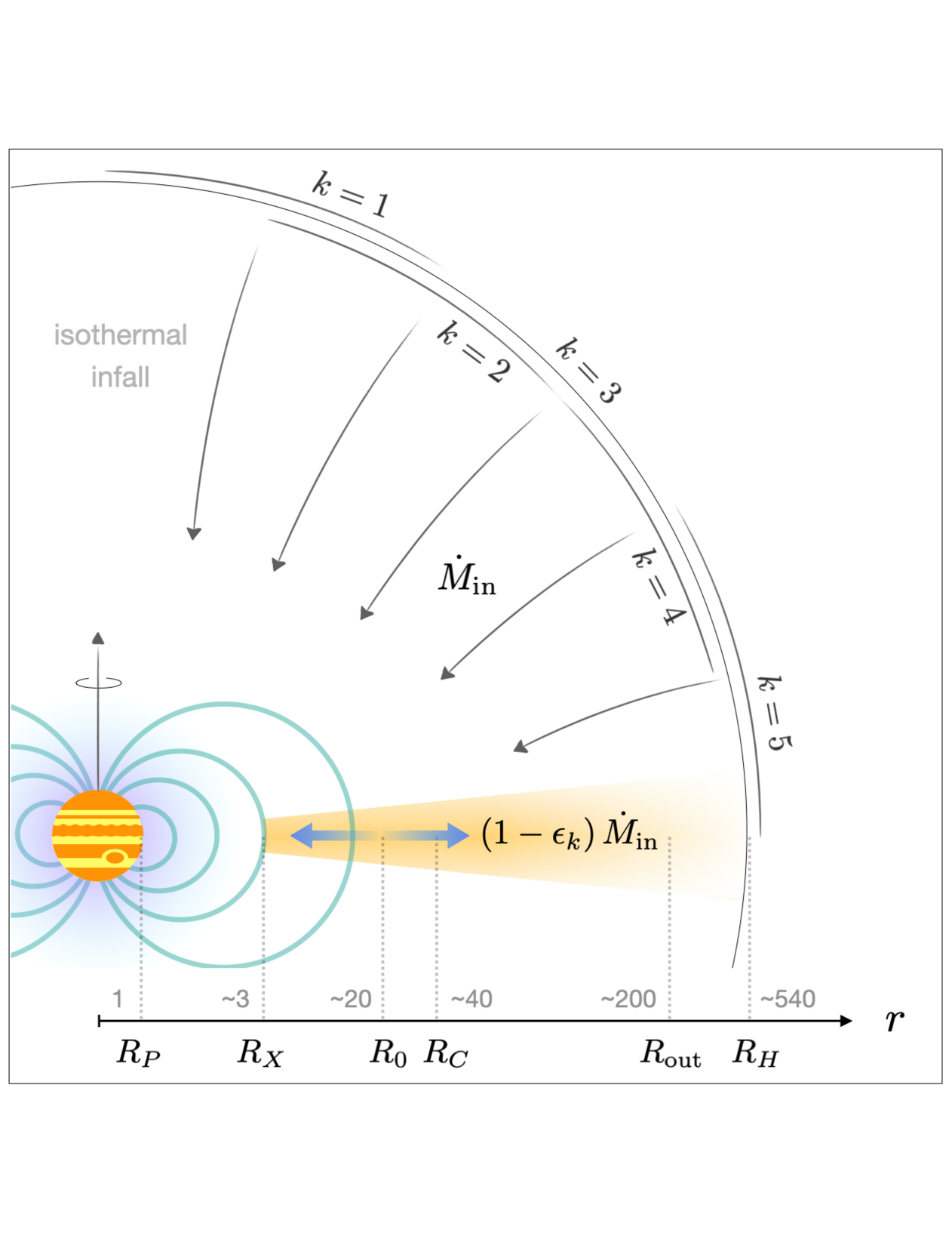
Figure 1: Schematic diagram of forming giant planet during the third stage of core accretion when most of the mass is accummulated. The background circumstellar disk feeds gas into the Hill sphere at a net rate ${\dot{M}}_{\rm in}$. The incoming material can have different angular distributions, indicated by the values of the index $k$. Infalling gas forms a circumplanetary disk, which in turn accretes mass onto the central planet with efficiency $\epsilon_{k}$. The length scales in the problem are shown along the lower horizontal axis, including the planet radius $R_{P}$, the magnetic truncation radius $R_{X}$ , the location $R_{0}$ where disk accretion changes sign, the centrifugal radius $R_{C}$, the outer disk radius $R_{\rm out}$, and finally the Hill radius $R_{H}$.

Although the mass flowing into the Hill sphere is expected to be rotating near the angular velocity of the local mean motion $\Omega$, the material that enters the vicinity of the planet often has a somewhat smaller effective rotation rate. This discepancy can be defined in terms of an angular momentum bias factor $\lambda<1$, defined so that the specific angular momentum in midplane is given by $J=\lambda\Omega R_{H}^{2}$. For the simplest case of undeflected, two-dimensional Keplerian flow, the angular momentum bias is estimated to be $\lambda=1/4$ (Lissauer & Kary, 1991). In general, however, the incoming trajectories will be influenced, at least in part, by pressure forces at large distances from the Hill sphere, and the resulting angular momentum bias is closer to unity (see, e.g., Ward & Canup 2010 for a more detailed discussion). In general, the bias factor is found to be an increasing function of the ratio $R_{B}/R_{H}$, so that it increases with the mass of the planet, and is expected to lie in the range $\lambda=1/3-1/2$. We note that existing calculations do not yet provide a definite prediction for this factor, and that additional physical considerations (e.g., magnetic fields) could affect the result. The analytic treatment of this paper provides solutions for any value of $\lambda$.

The angular distribution of material entering the Hill sphere has been studied through numerical simulations of the planet formation process (e.g., Tanigawa et al. 2012; Szulágyi 2017; Szulágyi & Mordasini 2017; Fung et al. 2019; and many others). Unfortunately, these studies do not yet provide an unambiguous specification of the expected angular dependence of the incoming material. Some simulations indicate that the flow enters the Hill sphere primarily along the rotational poles of the system (Lambrechts & Lega, 2017; Lambrechts et al., 2019), whereas other simulations suggest flow that is more concentrated toward the equatorial regions (Ayliffe & Bate, 2009). We also note that the angular dependence is likely to vary with the mass of the growing planet. For example, once the planet becomes large enough that its Hill sphere is larger than the scale height of the circumstellar disk, the incoming flow will become more equatorial. In light of these uncertainties, we consider a range of possible geometries (see Taylor & Adams 2024), ranging from flow focused along the poles with a factor $f\propto\cos^{2}\theta_{0}$, to isotropic with $f=1$, to flow primarily along equatorial directions with $f\propto\sin^{2}\theta_{0}$.

Next we need the orbital solutions for material entering the Hill sphere and falling toward the central planet and its circumplanetary disk. Past work used solutions developed earlier for star formation, where the orbits are taken to have zero energy, zero pressure, and where the starting radius is evaluated in the $r\to\infty$ limit (Ulrich, 1976; Cassen & Moosman, 1981; Chevalier, 1983; Terebey et al., 1984). Here we relax these assumptions (see also Mendoza et al. 2009) and construct orbit solutions evaluated at the finite outer boundary of the Hill radius. We also consider a range of solutions from zero total energy to vanishing radial velocity (at the boundary), noting that the latter approximation is more likely to hold.

A given orbit solution, corresponding to a particular set of boundary conditions at the Hill sphere, leads to a source term for the input of envelope material onto the evolving circumplanetary disk. For a given source term, the incoming material does not, in general, have the proper angular momentum to become part of the pre-existing circumplanetary disk (Cassen & Moosman, 1981; Cassen & Summers, 1983). As a result, the newly added material will adjust its energy, and hence is radial location within the disk, in a manner that conserves angular momentum and dissipates energy. This readjustment affects the evolution of the circumplanetary disk and its steady-state surface density profile.

Finally, in order to provide a proper accounting of the angular momentum budget for forming planets, we need to specify the outer boundary of the circumplanetary disk. Here the default assumption would be that the circumplanetary disk extends out to the Hill radius, where the potential of the background circumstellar disk must dominate. The Hill radius thus represents an upper limit to the outer boundary. In practice, the effective outer disk boundary falls at a smaller radius, $R_{\rm out}=\xi R_{H}$. At sufficiently large distances from the planet, the circumplanetary orbits become sufficiently non-circular so that they cross, dissipate energy, and can no longer support a coherent disk structure. Previous calculations indicate that $\xi\approx 2/5$ (Martin & Lubow, 2011).

The aforementioned numerical simulations highlight additional complications regarding the formation of circumplanetary disks and their host planets. Some of the material that initially enters the Hill sphere promptly flows back out (Machida et al., 2008; Lambrechts & Lega, 2017). In this paper, we consider the mass infall rate ${\dot{M}}_{\rm in}$ to represent the net rate at which material enters the Hill sphere (the difference between the mass rate inward and any outward flow). The analytic solutions found herein hold for any value of ${\dot{M}}_{\rm in}$, but its value is taken as a starting point (so that its calculation is beyond the scope of this work).

Another important complication involves the cooling rate of the incoming gas. A common thread through all numerical studies of circumplanetary hydrodynamics is the critical role of thermodynamics in circumplanetary disk formation. Numerical experiments (e.g., Szulágyi 2017; Fung et al. 2019; Krapp et al. 2024) consistently show that effective radiative cooling is required to shed the heat generated by accretion shocks and compressional heating – only then can gas settle into a rotationally supported disk. Without sufficient cooling, the gas remains nearly adiabatic and forms an envelope supported by pressure and entropy gradients instead of rotation. For example, global 3D radiative-hydrodynamics simulations (Klahr & Kley, 2006) showed that the forming planet was cocooned by a hot, pressure-supported envelope in lieu of a thin disk. More recent radiative simulations (Szulágyi et al., 2016) found that capping the temperature (to simulate cooling) was necessary to obtain a disk — implying a threshold in cooling efficiency below which a disk cannot form. Inefficient cooling also leads to recyling flows that channel a large fraction of gas through the Hill sphere without necessarily leading to disk formation (Lambrechts et al., 2019). Extending these results, Schulik et al. (2020) found a sharp transition near Saturn-to-Jupiter mass scales, where lower-mass protoplanets exhibit pressure-supported envelopes and higher-mass planets develop disks if cooling is sufficiently effective (see also Bailey et al. 2023). We emphasize here that in order for the system to accrete enough mass to produce a giant planet, the disk structure is necessary to transfer angular momentum outward and mass inward. In this paper, we thus consider only systems with sufficient cooling, where a disk and a planet can form (see Appendix A for additional discussion of this issue).

The analytic treatment of this paper complements existing numerical treatments of the problem. Despite tremendous advances, present-day simulations face significant limitations in capturing the full physics of circumplanetary disk formation. One major challenge is resolution: Resolving both the background disk environment and the planetary radius itself in one simulation is difficult with current computational resources. Even with nested grids or mesh refinement, the innermost flow near the planet is often smoothed or softened (e.g., Lega et al. 2024). Insufficient resolution can artificially suppress small-scale structures and can affect the measured accretion rates. For example, increasing the resolution around the planet significantly alters the disk temperature, luminosity, and density profile (Schulik et al., 2020), indicating that some simulations are not yet numerically converged. The time spans simulated (typically tens to hundreds of orbits) are short compared to those of actual planet formation (millions of years), making it difficult to examine a true steady state. Finally, computational costs force a trade-off between global realism and local detail: Global disk simulations have coarse resolution in the vicinity of the planet, whereas local ‘zoomed-in’ studies (e.g., Zhu et al. 2024) may not include large-scale flow features (e.g., the mass supply from the circumstellar disk). Due to these limitations, current simulations cannot fully account for the formation of a planet, disk, and envelope with all of the relevant physics. One goal of this paper is thus to fill in some these gaps with analytic solutions.

This paper calculates the form of the surface density for circumplanetary disks, which play an important role in determining the radiative signatures of forming planets. These systems are just now becoming observable (Benisty et al., 2021; Bae et al., 2022; Christiaens et al., 2024; Cugno et al., 2024). During planet formation, the disk dissipates significant energy and provides much of the luminosity. Compared to the planet itself, the radiation emanating from the disk is emitted at longer wavelengths, which are more easily observed. As more observations become available, more sophisticated theoretical models of the spectral energy distributions are warranted, and more accurate surface density distributions are required (see, e.g., Zhu 2015; Zhu et al. 2018; Szulágyi et al. 2019; Adams & Batygin 2022; Taylor & Adams 2025; Choksi & Chiang 2025).

This paper is organized as follows. Section 2 constructs the orbit solutions for the generalized case where the trajectories start at the (finite) Hill radius, have arbitrary angular momentum bias $\lambda$, and potentially non-zero starting radial velocity (although in practice the latter correction is small). Next we find the corresponding density distribution, velocity field, and source term for material falling onto the disk. The effects of angular momentum readjustment are derived in Section 3, resulting in the generalized equation of motion for the evolution of the circumplanetary disk. Steady-state solutions are found in Section 4, resulting in analytic expressions for the mass accretion rate and the surface density distribution as a function of radial position. Solutions are found for five choices of the inflow geometry, from polar to equatorial. These solutions, in turn, determine the fraction of the mass entering the disk that can accrete onto the planet, and thus determine the maximum accretion efficiency subject to conservation of angular momentum. The paper concludes, in Section 5, with a summary of our results and a discussion of their implications.

2 Generalized Infall Collapse Solutions

This section generalizes the standard collapse solution (Ulrich, 1976) to include more realistic choices for the outer boundary conditions. For the sake of definiteness, the solutions are fixed at the finite outer radius $R_{H}$ of the Hill sphere. For a given angular momentum, the radial velocity, and hence the energy, can be varied. The azimuthal velocity at the boundary is determined by the angular momentum, which is set by the bias parameter $\lambda$. For simplicity, we assume azimuthal symmetry and solid body rotation at the Hill sphere. In other words, the angular momentum bias $\lambda$ is taken to be a constant, rather than a function of polar angle $\theta_{0}$. Note that these assumptions could be relaxed in future work. We also note that at the latest evoluationary stages, the planet is expected to clear a wide gap in the background circumstellar disk, so that continued accretion onto the planet occurs through streamers (this accretion geometry will be addressed in future work).

Energy and angular momentum are conserved. In this formulation, the angular momentum of a parcel starting at radius $r=R_{H}$ and angle $\theta_{0}$ has the form

$$J=\lambda\Omega R_{H}^{2}\sin\theta_{0}\,,$$ (1)

where $\Omega^{2}=GM_{\ast}/a^{3}$ determines the rotation rate at the planet location, $\lambda$ is the angular momentum bias, and $\theta_{0}$ is the starting polar angle. The energy of the parcel is given by

$$E={1\over 2}v_{r}^{2}+{J^{2}\over 2r^{2}}-{GM\over r}\,,$$ (2)

where $r$ is the radial coordinate centered on the planet and the potential is that of a point mass $M$. The energy can be evaluated at the outer boundary, so we have

$$E=E_{0}={1\over 2}v_{H}^{2}+{J^{2}\over 2R_{H}^{2}}-{GM\over R_{H}}\,.$$ (3)

The angular momentum in this expression can be rewritten to take the form

$$J^{2}=\lambda^{2}\Omega^{2}R_{H}^{4}\sin^{2}\theta_{0}={1\over 3}\lambda^{2}GMR_{H}\sin^{2}\theta_{0}\,,$$ (4)

so that the energy becomes

$$E_{0}={1\over 2}v_{H}^{2}+{GM\over R_{H}}\left[{1\over 6}\lambda^{2}\sin^{2}\theta_{0}-1\right]\,.$$ (5)

Here we define a dimensionless energy

$$\epsilon\equiv E_{0}\left({GM\over R_{H}}\right)^{-1}={1\over 2}\eta^{2}+{1\over 6}\lambda^{2}\sin^{2}\theta_{0}-1\,,$$ (6)

where the dimensionless radial velocity $\eta$ (defined at the boundary) is given by

$$\eta^{2}={v_{H}^{2}R_{H}\over GM}\,.$$ (7)

In this treatment, the starting position is taken to be the Hill sphere ($r=R_{H}$) and the system is axisymmtric. The remaining initial spatial variable is the starting polar angle $\theta_{0}$. The angular momentum bias $\lambda$ determines the azimuthal speed in the orbit plane and the value of $\eta$ completes the specificiation of the initial condition (see also Mendoza et al. 2009).

The infalling parcel of gas executes an orbit in a plane that is tilted with respect to the spherical coordinate system centered on the planet with $\hat{z}$ axis along the pole. Within the tilted plane, the orbit equation has the usual form which can be written

$$u={\sin^{2}\theta_{0}\over 1-e\cos\varphi}\,,$$ (8)

where $\varphi$ is the azimuthal angle in the orbital plane and

$$u={r\over R_{C}}\qquad{\rm where}\qquad R_{C}={J^{2}(\pi/2)\over GM}={1\over 3}\lambda^{2}R_{H}\,.$$ (9)

The centrifugal radius is thus smaller than in the benchmark case (where $R_{C}=R_{H}/3$; Quillen & Trilling 1998) by a factor of $\lambda^{2}$. The eccentricity of the orbit can be determined from the definitions of energy and angular momentum of the orbit and takes the form

$$e^{2}=1+{2\over 3}\lambda^{2}\epsilon\sin^{2}\theta_{0}\,.$$ (10)

Next we use standard geometric rotations to write

$$\cos(\varphi-\varphi_{0})={\cos\theta\over\cos\theta_{0}}\qquad{\rm or}\qquad\varphi=\varphi_{0}+\cos^{-1}\left[{\cos\theta\over\cos\theta_{0}}\right]\,.$$ (11)

2.1 Effective Initial Disk Radius

Now consider the trajectory that leads to the largest radius that crosses the midplane, i.e., the effective disk radius. Note that this radius is the initial effective radius of the disk, which will subsequently spread outward due to the action of viscosity (see Section 4). Here we first take $\cos\theta=\mu=0$. The angle $\varphi$ is then given by

$$\varphi=\varphi_{0}+{\pi\over 2}\,,$$ (12)

so that

$$\cos\varphi=\cos(\varphi_{0})\cos(\pi/2)-\sin(\varphi_{0})\sin(\pi/2)=-\sin(\varphi_{0})\,.$$ (13)

If we evaluate the orbit equation at the outer boundary where $u=3/\lambda^{2}$ and $\varphi$ = $\varphi_{0}$, we can solve to find

$$e\cos\varphi_{0}=1-{1\over 3}\lambda^{2}\sin^{2}\theta_{0}\,.$$ (14)

We can use this expression to find $e\sin\varphi_{0}$. Using this result in conjunction with the expression of equation (10) for the eccentricity, we find that

$$e^{2}\sin^{2}\varphi_{0}=1+{2\over 3}\lambda^{2}\epsilon\sin^{2}\theta_{0}-\left[1-(\lambda^{2}/3)\sin^{2}\theta_{0}\right]^{2}\,.$$ (15)

After inserting the expression for the energy $\epsilon$, we find

$$e^{2}\sin^{2}\varphi_{0}=\eta^{2}\lambda^{2}\sin^{2}\theta_{0}/3\qquad{\rm or}\qquad e\sin\varphi_{0}=\eta\lambda\sin\theta_{0}/\sqrt{3}\,.$$ (16)

The orbit equation then takes the form

$$u={\sin^{2}\theta_{0}\over 1+\eta\lambda\sin\theta_{0}/\sqrt{3}}\,.$$ (17)

The nominal disk radius is set by the maximum value of $u$, which occurs for $\sin\theta_{0}=1$; these orbits start in the equatorial plane and have the largest specific angular momentum. The disk radius is thus given by

$$R_{\rm d}={R_{C}\over 1+\eta\lambda/\sqrt{3}}={\lambda^{2}R_{H}\over 3+\sqrt{3}\lambda\eta}\,.$$ (18)

The disk radius can be somewhat smaller than the centrifugal radius, although we expect both $\eta$ and $\lambda$ to be small, so the correction in the denominator is modest.

2.2 Limit of Zero Initial Radial Velocity

The starting velocity at the Hill sphere is expected to be relatively small. For example, if we take $v_{H}$ to be the sound speed, then $\eta^{2}\sim 0.07$ for Jovian planets forming near the ice line. The kinetic energy from the radial velocity is thus only $\sim 3.5\%$ of the gravitational potential energy. This small value for the starting velocity motivates us to consider the limiting case where $\eta\to 0$. In this limit, the energy is given by

$$\epsilon={1\over 6}\lambda^{2}\sin^{2}\theta_{0}-1\,,$$ (19)

and the eccentricity is given by

$$e^{2}=1+{2\over 3}\lambda^{2}\sin^{2}\theta_{0}\left[{1\over 6}\lambda^{2}\sin^{2}\theta_{0}-1\right]=\left[1-{1\over 3}\lambda^{2}\sin^{2}\theta_{0}\right]^{2}\,,$$ (20)

so that

$$e=1-{1\over 3}\lambda^{2}\sin^{2}\theta_{0}\,.$$ (21)

If we evaluate the orbit equation at the boundary to specify the starting angle $\varphi_{0}$, we find

$$1-\left[1-{1\over 3}\lambda^{2}\sin^{2}\theta_{0}\right]\cos\varphi_{0}={1\over 3}\lambda^{2}\sin^{2}\theta_{0}\qquad\Rightarrow\qquad\cos\varphi_{0}=1\,,$$ (22)

or, equivalently, $\varphi_{0}=0$. The general form of the orbit equation thus becomes

$$1-\left[1-{1\over 3}\lambda^{2}(1-\mu_{0}^{2})\right]{\mu\over\mu_{0}}={1\over u}(1-\mu_{0}^{2})\,.$$ (23)

To find the disk radius, we can evaluate this expression at $\mu=0$, and then take the limit $\mu_{0}\to 0$ to find

$$u=1\qquad\Rightarrow\qquad R_{\rm d}=R_{C}\,.$$ (24)

In this limit, we can also find the radial location $u_{d}$ where incoming trajectories strike the disk. Evaluating the orbit equation in the limit $\mu\to 0$, we find the standard result,

$$u_{d}(\mu_{0})=1-\mu_{0}^{2}\,,$$ (25)

i.e., the same as before in the Ulrich limit (but not for the case with $\eta\neq 0$).

The solutions of this subsection are carried out in the limit $\eta\to 0$. To quantify the severity of this assumption, one can consider how nonzero radial velocity affects the nominal disk size. Suppose that the radial velocity at the Hill sphere is given by the local Keplerian shear so that $v_{H}=\Omega R_{H}$ and $\eta^{2}=1/3$. In this case, the nominal disk radius is no longer given by equation (24), but rather by equation (18) with $\eta\neq 0$. The relative difference in disk radius can be written

$${\Delta R_{\rm d}\over R_{\rm d}}={\lambda\eta\over\sqrt{3}+\lambda\eta}\rightarrow{1\over 7}\,,$$ (26)

where the final equality holds for $\eta=1/\sqrt{3}$ and for an angular momentum bias $\lambda=1/2$. The correction due to nonzero starting radial velocities is thus modest. For completeness, note that infall solutions with $\eta\neq 0$ can be readily constructed, although the expressions become much more complicated (Adams & Batygin – unpublished). We leave a more general treatment of this problem for future work (see also Mendoza et al. 2009).

2.3 Velocity Fields

We can find the velocity fields by applying conservation of angular momentum and energy. The azimuthal velocity is given by conservation of the $\hat{z}$ compontent of angular momentum,

$$v_{\phi}={J_{z}\over r\sin\theta}\qquad{\rm where}\qquad J_{z}=\lambda\Omega R_{H}^{2}\sin^{2}\theta_{0}=\sqrt{GMR_{C}}\sin^{2}\theta_{0}\,,$$ (27)

so we find

$$v_{\phi}=\left({GM\over R_{C}}\right)^{1/2}{R_{C}\over r}{\sin^{2}\theta_{0}\over\sin\theta}\,.$$ (28)

Similarly, the velocity component $v_{\theta}$ is determined by requiring conservation of total angular momentum, i.e.,

$$r^{2}(v_{\theta}^{2}+v_{\phi}^{2})=J_{T}^{2}=GMR_{C}\sin^{2}\theta_{0}\,.$$ (29)

Using the previous result, we find

$$v_{\theta}=\left({GM\over R_{C}}\right)^{1/2}{R_{C}\sin\theta_{0}\over r\sin\theta}\left[\cos^{2}\theta_{0}-\cos^{2}\theta\right]^{1/2}\,.$$ (30)

Note that equation (28) and (30) were derived using conservation of angular momentum, and we did not need to invoke conservation of energy. As a result, these expressions are valid for all choices of the orbital energy.

For the radial velocity component, we need to specify the orbital energy or equivalently the value of $\eta$. The energy is given by

$$E_{0}={1\over 2}v_{H}^{2}+{GM\over R_{H}}\left[{1\over 6}\lambda^{2}\sin^{2}\theta_{0}-1\right]={GM\over 2R_{H}}\left[\eta^{2}+{1\over 3}\lambda^{2}\sin^{2}\theta_{0}-2\right]\,.$$ (31)

The radial velocity thus takes the form

$$v_{r}=\left({GM\over R_{C}}\right)^{1/2}\left\{{1\over 3}\lambda^{2}\left[\eta^{2}+{1\over 3}\lambda^{2}\sin^{2}\theta_{0}-2\right]-\zeta^{2}\sin^{2}\theta_{0}+2\zeta\right\}^{1/2}\,.$$ (32)

In the limit of zero initial velocity, the expression becomes

$$v_{r}=\left({GM\over R_{C}}\right)^{1/2}\left\{{1\over 3}\lambda^{2}\left[{1\over 3}\lambda^{2}\sin^{2}\theta_{0}-2\right]-\zeta^{2}\sin^{2}\theta_{0}+2\zeta\right\}^{1/2}\,.$$ (33)

2.4 Source Term for Infall onto the Disk

In order to specify the flow of material onto the circumplanetary disk, we need to evalute the source term

$${\cal S}=\left[2\rho v_{\theta}\right]_{\mu=0}\,.$$ (34)

We thus need to evalute the density and the velocity component $v_{\theta}$ as the parcels of gas cross the midplane. The density is given by conservation of mass along streamtubes, i.e.,

$$\rho={{\dot{M}}_{\rm in}f(u)\over 4\pi r^{2}|v_{r}|}{d\mu_{0}\over d\mu}\,,$$ (35)

where all quantities are evaluated at $\mu=0$. The total net rate of mass infall onto the disk is ${\dot{M}}_{\rm in}$, and the function $f(u)$ accounts for the angular dependence. More specifically, $f(u)$ = 1 for isotropic infall, but takes on non-constant forms for infall patterns with angular dependence (see Section 4).

The polar velocity $v_{\theta}$ is given by equation (30), which can be evaluated to obtain

$$v_{\theta}\Big{|}_{\mu=0}=\left({GM\over R_{C}}\right)^{1/2}{R_{C}\over r}\sin\theta_{0}\cos\theta_{0}\,,$$ (36)

where the orbit equation determines $\theta_{0}$. In the limit of zero starting velocity, the orbit equation can be evaluated at the midplane $\mu=0$ (see equation [25]) to obtain $u=(1-\mu_{0}^{2})$ or $\mu_{0}^{2}=1-u$. The derivative $d\mu_{0}/d\mu$ thus takes the form

$${d\mu_{0}\over d\mu}={u\over 2\mu_{0}^{2}}\left[1-{1\over 3}\lambda^{2}(1-\mu_{0}^{2})\right]={u\over 2}{(1-\lambda^{2}u/3)\over(1-u)}\,.$$ (37)

The polar velocity becomes

$$v_{\theta}\Big{|}_{\mu=0}=\left({GM\over R_{C}}\right)^{1/2}{R_{C}\over r}\sqrt{u}\sqrt{1-u}=\left({GM\over r}\right)^{1/2}\sqrt{1-u}\,,$$ (38)

and the radial velocity becomes

$$v_{r}=\left({GM\over R_{C}}\right)^{1/2}\left\{{1\over 3}\lambda^{2}\left[{1\over 3}\lambda^{2}u-2\right]+\zeta\right\}^{1/2}=\left({GM\over r}\right)^{1/2}(1-\lambda^{2}u/3)\,.$$ (39)

After putting the pieces together, we can write the source term in the form

$${\cal S}=2{{\dot{M}}_{\rm in}f(u)\over 4\pi r^{2}}{\sqrt{1-u}\over 1-\lambda^{2}u/3}\left({u\over 2}\right){(1-\lambda^{2}u/3)\over(1-u)}={{\dot{M}}_{\rm in}\over 4\pi r^{2}}{uf(u)\over\sqrt{1-u}}\,.$$ (40)

3 Disk Surface Density with Angular Momentum Adjustment

The continuity equation for the surface density of the disk (e.g., Shu 1990) can be written in the form

$${\partial\Sigma\over\partial t}={1\over 2\pi r}{\partial{\dot{M}}\over\partial r}+\left[2\rho v_{\theta}\right]_{\mu=0}\,,$$ (41)

where the final term is the source due to infall from the protoplaneary envelope onto the disk and is given by equation (40). In this formulation, the quantity ${\dot{M}}$ is the mass accretion rate through the disk (as a function of $r$ in the disk) and ${\dot{M}}_{\rm in}$ is the mass accretion rate onto the entire disk (from the envelope).

In addition to convervation of mass (41), angular momentum must also be conserved. If we consider the increment of angular momentum in a box surrounding an annulus of the disk, we have

$$dJ_{T}=2\pi r\Sigma\Gamma dr\qquad{\rm where}\qquad\Gamma=\sqrt{GM_{0}r}\,,$$ (42)

where the specific angular momentum $\Gamma$ of the disk material is assumed to be Keplerian with a source mass $M_{0}$. The time rate of change of the angular momentum is then given by

$${\partial\over\partial t}\left[2\pi r\Sigma\Gamma\right]=2\pi r{\cal S}\gamma_{\rm in}+{\partial\over\partial r}\left[{\dot{M}}\Gamma\right]+{\partial{\cal T}\over\partial r}\,,$$ (43)

where $\gamma_{\rm in}$ is the specific angular momentum of the incoming material, and where the torque ${\cal T}$ due to disk viscosity $\nu$ (Shu, 1990; Hartmann, 2009) is given by

$${\cal T}=(2\pi r)\Sigma\nu r^{2}{d\Omega\over dr}\,.$$ (44)

The specific angular momentum of the incoming material is given by

$$\gamma_{\rm in}=\left[rv_{\phi}\right]_{\mu=0}=\sqrt{GM_{0}r}\sqrt{u}=\sqrt{GM_{0}R_{C}}\,u\,.$$ (45)

After some rearrangement, we can write the continuity equation (multiplied by $\Gamma$) and the conservation of angular momentum equation in the forms:

$$2\pi r\Gamma{\partial\Sigma\over\partial t}=\Gamma{\partial{\dot{M}}\over\partial r}+2\pi r{\cal S}\Gamma\,,$$ (46)

and

$$2\pi r{\partial\over\partial t}\left[\Sigma\Gamma\right]=2\pi r{\cal S}\gamma_{\rm in}+{\partial\over\partial r}\left[{\dot{M}}\Gamma\right]+{\partial{\cal T}\over\partial r}\,.$$ (47)

These two equations can be combined and then solved for the mass accretion rate ${\dot{M}}$ to find

$${\dot{M}}=4\pi r^{2}\Sigma{{\dot{M}}_{\rm in}\over 2M_{0}}-4\pi r^{2}{\cal S}(\sqrt{u}-1)-{2r\over\Gamma}{\partial{\cal T}\over\partial r}\,.$$ (48)

Now take the derivative with respect to the radial coordinate $r$, and divide by $2\pi r$ to get

$${1\over 2\pi r}{\partial{\dot{M}}\over\partial r}={{\dot{M}}_{\rm in}\over M_{0}}\left[r{\partial\Sigma\over\partial r}+2\Sigma\right]+{3\over r}{\partial\over\partial r}\left(\sqrt{r}{\partial\over\partial r}\left[\sqrt{r}\nu\Sigma\right]\right)+{\cal S}\left({2-\sqrt{u}-2u\over 1+\sqrt{u}}+(1-\sqrt{u}){2u\over f}{df\over du}\right)$$ (49)

Using this result in equation (41) gives us the equation of motion for the evolution of the surface density of the disk

$${\partial\Sigma\over\partial t}={{\dot{M}}_{\rm in}\over M_{0}}\left[r{\partial\Sigma\over\partial r}+2\Sigma\right]+{3\over r}{\partial\over\partial r}\left(\sqrt{r}{\partial\over\partial r}\left[\sqrt{r}\nu\Sigma\right]\right)+{\cal S}\left({3-2u\over 1+\sqrt{u}}+(1-\sqrt{u}){2u\over f}{df\over du}\right)\,.$$ (50)

The time derivative operator corresponds to the case where $r$ is held constant. In order to construct the solution for the case where $u$ is held constant, we need another term in the time derivative to take into account the time variation of the centrifugal radius, i.e.,

$${\partial\Sigma\over\partial t}\Bigg{|}_{r}={\partial\Sigma\over\partial t}\Bigg{|}_{u}+{\partial\Sigma\over\partial u}{\partial u\over\partial t}={\partial\Sigma\over\partial t}\Bigg{|}_{u}-u{\partial\Sigma\over\partial u}{{\dot{R}}_{C}\over R_{C}}\,.$$ (51)

We can now write the partial differential equation for $\Sigma(u,t)$ in the form

$${\partial\Sigma\over\partial t}={{\dot{M}}_{\rm in}\over M_{0}}2\Sigma+u{\partial\Sigma\over\partial u}\left[{{\dot{M}}_{\rm in}\over M_{0}}+{{\dot{R}}_{C}\over R_{C}}\right]+{3\over R_{C}^{2}}{1\over u}{\partial\over\partial u}\left(\sqrt{u}{\partial\over\partial u}\left[\sqrt{u}\nu\Sigma\right]\right)$$ (52)

$$+{{\dot{M}}_{\rm in}\over 4\pi R_{C}^{2}}{f(1-\sqrt{u})\over u\sqrt{1-u}}\left({3-2u\over 1-u}+{2u\over f}{df\over du}\right)\,.$$

To complete the specification of the problem, we need to enforce boundary conditions. In the limit of small radius $r\to 0$, the mass accretion rate must approach a constant value (in the inward direction). The inner boundary should be enforced at the inner truncation radius, which is set by the magnetic field strength on the planetary surface (Ghosh & Lamb, 1978; Blandford & Payne, 1982). In practice, however, we can enforce the inner boundary in the limit $r\to 0$. At the outer disk edge, the mass accretion is outward, and must have the value required to remove essentially all of the incoming angular momentum from the system. We thus assume that the angular momentum carried by the planetary rotation is negligible compared to the total angular momentum entering the planet/disk system.

4 Steady-State Solutions

In this section we consider steady state solutions for the surface density of the circumplanetary disk. These solutions are valid in the limit where the time scale for disk evolution due to viscosity $t_{\nu}\sim R_{C}^{2}/\nu$ is shorter than the evolution time $t_{\rm in}\sim M/{\dot{M}}_{\rm in}$. This ordering holds as long as the disk viscosity parameter $\alpha\,\raise 1.29167pt\hbox{$>$}\kern-7.5pt\lower 3.01385pt\hbox{$\sim$}\,10^{-4}$ (Adams & Batygin, 2022), where this requirement is likely to be realized (see Lesur et al. 2023 for a recent review). In this limit, the planet mass will be large compared to the mass of the circumplanetary disk. As a result, we can use a single mass scale $M$ for the planet mass, the source mass for Keplerian orbits in the disk, and the mass of the point potential that determines the incoming trajectories.

For the case of interest where the infall has angular dependence, we consider models where the incoming flow at the Hill sphere depends on initial polar angle according to $f_{1}\propto\cos^{2}\theta_{0}$, $f_{2}\propto\cos\theta_{0}$, $f_{3}=1$, $f_{4}\propto\sin\theta_{0}$, and $f_{5}\propto\sin^{2}\theta_{0}$ (Taylor & Adams, 2024). The corresponding disk input function has additional dependence on the radial coordinate. In terms of the variable $u=r/R_{C}$, the resulting functions $f_{k}(u)$ are given by

$$f_{1}=3(1-u)\,,\qquad f_{2}=2(1-u)^{1/2}\,,\qquad f_{3}=1\,,\qquad f_{4}={4\over\pi}\sqrt{u}\,,\qquad f_{5}={3\over 2}u\,.$$ (53)

For these infall geometries, the amount of incoming angular momentum is given by the dimensionless factors

$${\cal F}_{k}\equiv{[{\dot{J}}_{\rm in}]\over{\dot{M}}_{\rm in}\sqrt{GMR_{C}}}=2/5,\quad 1/2,\quad 2/3,\quad 3/4,\quad{\rm and}\quad 4/5\,,$$ (54)

where the sequence goes from more polar (with index $k=1$) to isotropic $(k=3)$ to more equatorial $(k=5)$.

Here we apply the outer boundary condition at $u_{\rm out}$, where the required outgoing accretion rate is determined by the fractions from equation (54). As a result, the efficiency of mass accretion increases as the incoming flow becomes more concentrated along the poles. The dimensionless outer boundary is given by $u_{\rm out}$ = $R_{\rm out}/R_{C}$ = $3\xi/\lambda^{2}$, where we expect $\xi\approx 2/5$ and $\lambda$ = 1/3 – 1/2. As a result, we take $u_{\rm out}=5$ as a benchmark value (although the expressions derived below hold for all values).

In steady state, to leading order, the equation of motion for the disk takes the form

$${\cal S}\left[{3-2u\over 1+\sqrt{u}}+(1-\sqrt{u}){2u\over f}{df\over du}\right]+{3\over R_{C}^{2}}{1\over u}{\partial\over\partial u}\left(\sqrt{u}{\partial\over\partial u}\left[\sqrt{u}\nu\Sigma\right]\right)=0\,,$$ (55)

where we drop the subscript on the function $f(u)$. If we define a dimensionless mass accretion rate $\gamma$ according to

$$\gamma={6\pi\over{\dot{M}}_{\rm in}}\left(\sqrt{u}{\partial\over\partial u}\left[\sqrt{u}\nu\Sigma\right]\right)\,,$$ (56)

the equation of motion takes the form

$${\partial\gamma\over\partial u}=-{f(u)\over 2}\left[{(1-\sqrt{u})(3-2u)\over(1-u)^{3/2}}+{(1-\sqrt{u})\over\sqrt{1-u}}{2u\over f}{df\over du}\right]\,.$$ (57)

For the five cases of interest, right hand side of the equation depends on $f(u)$, as given above, and the corresponding derivatives

$${2u\over f}{df\over du}=-{2u\over 1-u}\,,\qquad-{u\over 1-u}\,,\qquad 0\,,\qquad 1\,,\qquad{\rm and}\qquad 2\,.$$ (58)

4.1 Polar Flow

For polar flow, where ${\dot{M}}_{\rm in}\propto\cos^{2}\theta_{0}$ and index $k=1$, the equation of motion becomes

$${\partial\gamma\over\partial u}=-{3\over 2}{(1-\sqrt{u})\over(1-u)^{1/2}}(3-4u)\,,$$ (59)

which can be integrated to obtain

$$\gamma=\gamma_{\rm in}-1+\sqrt{1-u}\left(1-4u+3u^{3/2}\right)\Theta(1-u)\,,$$ (60)

where $\Theta(x)$ is the Heaviside step function (Abramowitz & Stegun, 1972). In the limit $u\to 0$, the dimensionless mass accretion rate becomes $\gamma_{\rm in}$. Beyond $u>1$, the source term vanishes, and the accretion rate $\gamma$ becomes constant with value given by

$$\gamma=\gamma_{\rm out}=\gamma_{\rm in}-1\,.$$ (61)

In order to conserve angular momentum, so that the outward flow of angular momentum at the outer boundary accounts for all of the incoming angular momentum, one needs

$$\gamma_{\rm out}\sqrt{u_{\rm out}}=-{2\over 5}\qquad\Rightarrow\qquad\gamma_{\rm in}-1=-{2\over 5\sqrt{u_{\rm out}}}\,.$$ (62)

We can integrate the mass accretion rate to find the surface density profile:

$$\sqrt{u}\nu\Sigma={{\dot{M}}_{\rm in}\over 6\pi}\int_{0}^{u}\gamma(u)u^{-1/2}du\,,$$ (63)

which gives us

$$\Sigma={{\dot{M}}_{\rm in}\over 6\pi\nu_{C}}u^{-3/2}\left\{{4\over 5}-{4\sqrt{u}\over 5\sqrt{u_{\rm out}}}-{2\over 5}\sqrt{1-u}\,(1-\sqrt{u})^{2}(2-\sqrt{u}-3u)\Theta(1-u)\right\}\,.$$ (64)

4.2 Quasipolar Flow

For the case where ${\dot{M}}_{\rm in}\propto\cos\theta_{0}$ and index $k=2$, the equation of motion becomes

$${\partial\gamma\over\partial u}=-3(1-\sqrt{u})\,,$$ (65)

which can be integrated to obtain

$$\gamma=\gamma_{\rm in}-1+(1-\sqrt{u})^{2}(1+2\sqrt{u})\Theta(1-u)\,.$$ (66)

In the limit $u\to 0$, the dimensionless mass accretion is thus $\gamma_{\rm in}$. Beyond $u>1$, $\gamma$ becomes constant, and we apply the outer boundary condition as before. After integrating a second time, the surface density takes the form

$$\Sigma={{\dot{M}}_{\rm in}\over 6\pi\nu_{C}}u^{-3/2}\left\{1-\sqrt{u/u_{\rm out}}+(2\sqrt{u}-2u^{3/2}+u^{2}-1)\Theta(1-u)\right\}\,.$$ (67)

4.3 Isotropic Flow

For the case of isotropic flow, the function $f=1$, the index $k=3$, and the equation of motion becomes

$${\partial\gamma\over\partial u}=-{1\over 2}{(1-\sqrt{u})(3-2u)\over(1-u)^{3/2}}\,,$$ (68)

which can be integrated to find

$$\gamma=\gamma_{\rm in}-1+\sqrt{1-u}{1+\sqrt{u}-u\over 1+\sqrt{u}}\Theta(1-u)\,.$$ (69)

Integrating again yields the surface density

$$\Sigma={{\dot{M}}_{\rm in}\over 9\pi\nu_{C}}u^{-3/2}\left[2-2\sqrt{u\over u_{\rm out}}-\sqrt{1-u}(2-3\sqrt{u}+u)\Theta(1-u)\right]\,.$$ (70)

4.4 Quasiequatorial Flow

For the case where ${\dot{M}}_{\rm in}\propto\sin\theta_{0}$ and index $k=4$, the equation of motion takes the form

$${\partial\gamma\over\partial u}=-{2\over\pi}\sqrt{u}\left[{(1-\sqrt{u})(3-2u)\over(1-u)^{3/2}}+{(1-\sqrt{u})\over\sqrt{1-u}}\right]=-{2\over\pi}\sqrt{u}{(1-\sqrt{u})(4-3u)\over(1-u)^{3/2}}\,.$$ (71)

After integrating we find

$$\gamma=\gamma_{\rm in}-1+{2\over\pi}\left\{{(1+\sqrt{u}-2u)(u-u^{2})^{1/2}\over 1+\sqrt{u}}+{\pi\over 2}-{\rm ArcSin}\sqrt{u}\right\}\Theta(1-u)\,.$$ (72)

Applying the boundary conditions and integrating allows us to write the surface density in the form

$$\Sigma={{\dot{M}}_{\rm in}\over 6\pi\nu_{C}}u^{-3/2}\Biggl{[}{3\over 2}(1-\sqrt{u/u_{\rm out}})+\Biggl{\{}2\sqrt{u}+{1\over\pi}\Biggl{[}\sqrt{1-u}(-3\sqrt{u}+4u-2u^{3/2})$$ (73)

$$-3{\rm ArcCos}\sqrt{u}-4\sqrt{u}{\rm ArcSin}\sqrt{u}\Biggr{]}\Biggr{\}}\Theta(1-u)\Biggr{]}$$

4.5 Equatorial Flow

For this case, ${\dot{M}}_{\rm in}\propto\sin^{2}\theta_{0}$ and the index $k=5$, so that the equation of motion becomes

$${\partial\gamma\over\partial u}=-{3u\over 4}\left[{(1-\sqrt{u})(5-4u)\over(1-u)^{3/2}}\right]\,,$$ (74)

which integrates to the form

$$\gamma=\gamma_{\rm in}-1+{\sqrt{1-u}(2+2\sqrt{u}+u+u^{3/2}-3u^{2})\over 2(1+\sqrt{u})}\Theta(1-u)\,.$$ (75)

After integrating and applying the boundary conditionsm, the surface density takes the form

$$\Sigma={{\dot{M}}_{\rm in}\over 30\pi\nu_{C}}u^{-3/2}\left\{8-8\sqrt{{u\over u_{\rm out}}}+\sqrt{1-u}\left(-8+10\sqrt{u}-4u+5u^{3/2}-3u^{2}\right)\Theta(1-u)\right\}\,.$$ (76)

4.6 Summary

All of the surface density profiles found in the previous subsections can be written in the general form

$$\Sigma(r)={{\dot{M}}\over 6\pi\nu}s_{k}(u)={{\dot{M}}\over 6\pi\nu_{C}}u^{-1}s_{k}(u)\,,$$ (77)

where the functions $s_{k}(u)$ depend on the flow geometry. It is useful to collect the results for the reduced surface density profiles $s_{k}(u)$ for the five cases:

$$s_{1}(u)=u^{-1/2}\left\{{4\over 5}-{4\sqrt{u}\over 5\sqrt{u_{\rm out}}}-{2\over 5}\sqrt{1-u}\,(1-\sqrt{u})^{2}(2-\sqrt{u}-3u)\Theta(1-u)\right\}\,,$$ (78)

$$s_{2}(u)=u^{-1/2}\left\{1-{\sqrt{u}\over\sqrt{u_{\rm out}}}+(2\sqrt{u}-2u^{3/2}+u^{2}-1)\Theta(1-u)\right\}\,,$$ (79)

$$s_{3}(u)=u^{-1/2}{2\over 3}\left\{2-2{\sqrt{u}\over\sqrt{u_{\rm out}}}-\sqrt{1-u}(2-3\sqrt{u}+u)\Theta(1-u)\right\}\,,$$ (80)

$$s_{4}(u)=u^{-1/2}\Biggl{\{}{3\over 2}-{3\over 2}{\sqrt{u}\over\sqrt{u_{\rm out}}}+\Biggl{\{}2\sqrt{u}+{1\over\pi}\Biggl{[}\sqrt{1-u}(-3\sqrt{u}+4u-2u^{3/2})$$

$$-3{\rm ArcCos}\sqrt{u}-4\sqrt{u}{\rm ArcSin}\sqrt{u}\Biggr{]}\Biggr{\}}\Theta(1-u)\Biggr{\}}\,,$$ (81)

and finally

$$s_{5}(u)=u^{-1/2}{1\over 5}\left\{8-8{\sqrt{u}\over\sqrt{u_{\rm out}}}+\sqrt{1-u}\left(-8+10\sqrt{u}-4u+5u^{3/2}-3u^{2}\right)\Theta(1-u)\right\}\,.$$ (82)

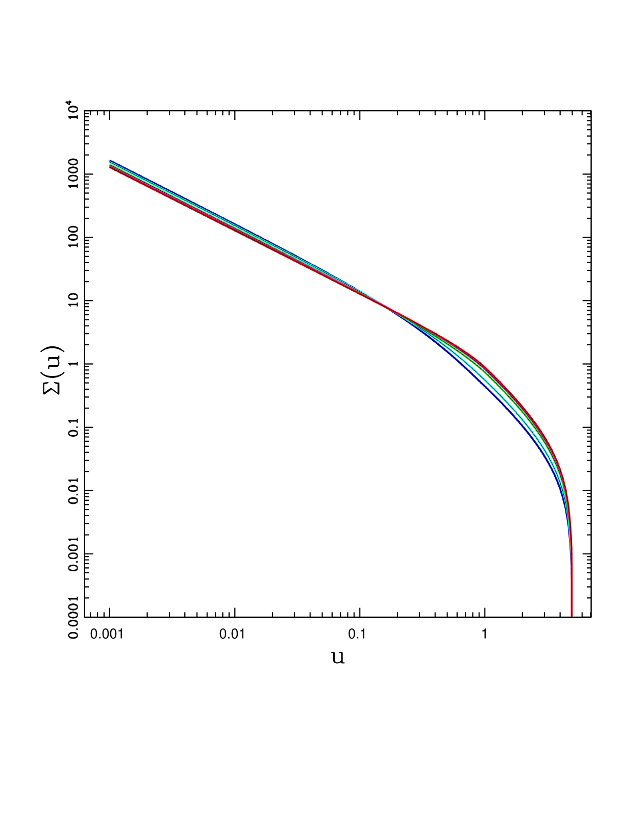
Figure 2: Surface density distributions for circumplanetary disk being fed by varying infall patterns, from polar (top blue curve on the left) to isotropic (middle green curve) to equatorial (bottom red curve on the left). Here the outer boundary is specified by $u_{\rm out}$ = $3\xi/\lambda^{2}$ = 5 (so that $\lambda\sim 1/2$).

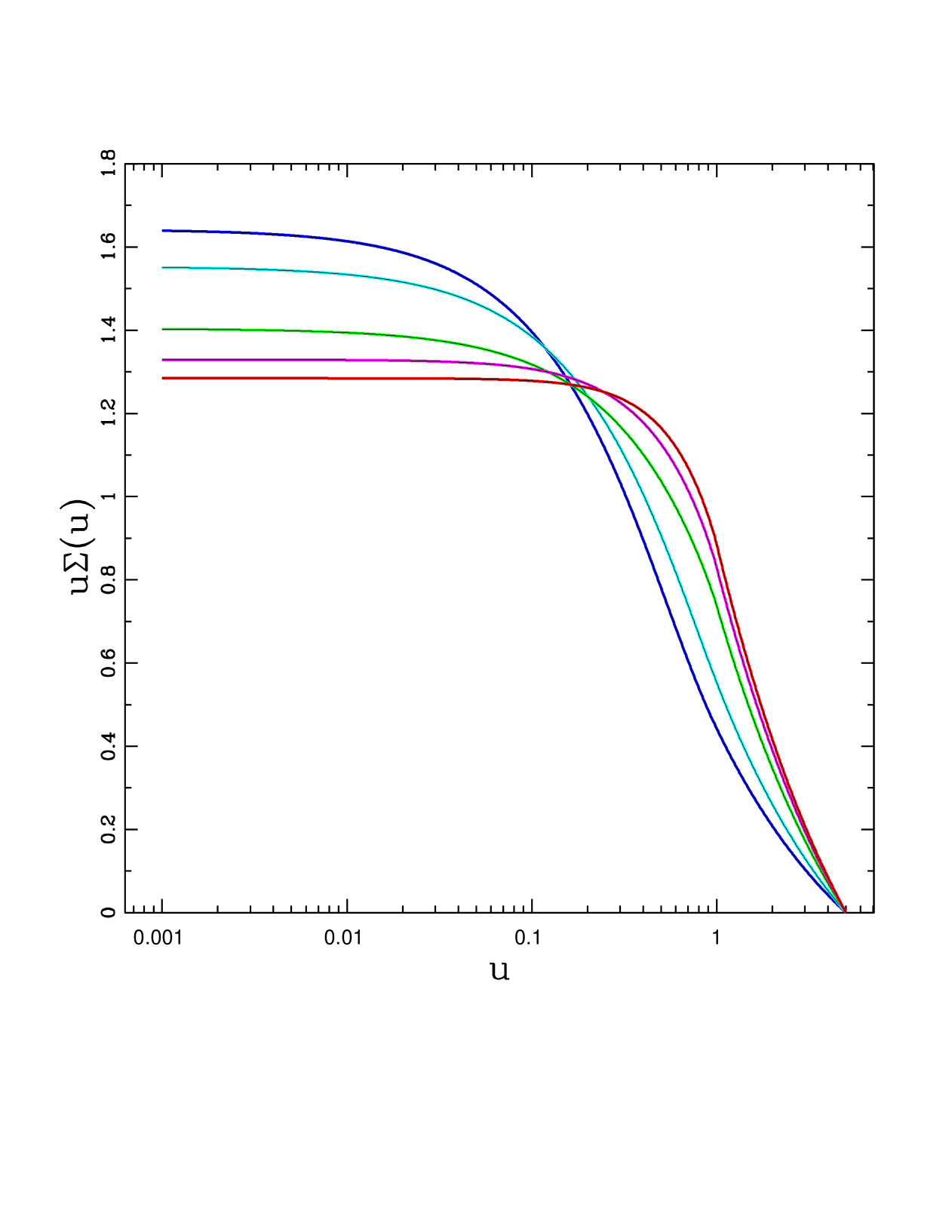
Figure 3: Surface density distributions for circumplanetary disk scaled by one power of the radial coordinate. The various curves correspond to different infall patterns, from polar (top blue curve on the left) to isotropic (middle green curve) to equatorial (bottom red curve on the left). Here the outer boundary is specified by $u_{\rm out}$ = $3\xi/\lambda^{2}$ = 5 (so that $\lambda\sim 1/2$).

The surface density profiles are depicted in Figures 2 and 3 for the five flow geometries under consideration. Figure 2 shows the surface density itself, in dimensionless form, i.e., the functions $u^{-1}s_{k}(u)$ for $k$ = 1 – 5. These forms are valid for any choice of the mass infall rate ${\dot{M}}_{\rm in}$, viscosity scale $\nu_{C}$ (and $\alpha$), and angular momentum bias $\lambda$ (which sets the centrifugal radius $R_{C}$). To leading order, the surface density distributions show simple power-law behavor $\Sigma\propto 1/u$ in the inner regions, with a cutoff at the outer disk edge (here at $u_{\rm out}$ = 5). The departures from a power-law form are necessary to reach a steady-state configuration for the given source functions, and to satisfy the outer boundary condition. Figure 3 shows the corresponding profiles scaled by one power of radius, i.e., the functions $s_{k}(u)$. These scaled profiles reach a constant value in the inner regions ($u\to 0$), where the value is proprotional to the accretion efficiency (see equation [89]). In both figures, the colors depict the results for the different input geometries, varying from polar (top blue curve) to isotropic (middle green curve) to equatorial (bottom red curve).

Figure 4 shows the effects of varying the angular momentum bias factor $\lambda$ and the location of the disk outer boundary as determined by $\xi$ (recall that $R_{\rm out}=\xi R_{H}$). The scaled surface denisty $r\Sigma$ is plotted versus $r/R_{H}$, where the radius is shown on a logarithmic scale. For simplicity, surface density distributions are shown for the case of steady-state evolution and an isotropic infall pattern. In the figure, the three colored curves depict the surface density distributions for angular momentum bias values $\lambda$ = 1 (green), 1/2 (blue), and 1/4 (red). For all three profiles, the outer boundary is held constant at $R_{\rm out}=2R_{H}/5$. As the angular momentum bias factor decreases, the surface density increases at small radii, and the profile decreases more rapidly with $r$, thereby leading to an effectively steeper density distribution. In order to illustrate how the surface density profiles depend on the outer boundary condition, the black curves show profiles with fixed angular momentum bias $\lambda$ = 1, and varying values of $\xi$ = 1 (upper solid curve), 0.8 (middle dashed curve), and 0.6 (lower dashed curve). Note that the green curve (with $\lambda$ = 1 and $\xi$ = 0.4) continues the sequence. The square symbols show the locations of the centrifugal radius $R_{C}$ for each case (where $R_{C}/R_{H}=\lambda^{2}/3$). As the location of the outer boundary moves inward, the scaled surface density profile decreases by an overall factor, but retains essentially the same shape.

Although the surface density profiles found here (equations [78 – 82]) are expressed in terms of elementary functions, their forms remain somewhat complicated. For some applications, even simpler approximations are useful. Toward this end, Appendix B presents a straightforward approximation scheme that captures the basic properties of these solutions (including how the profiles vary with infall geometry).

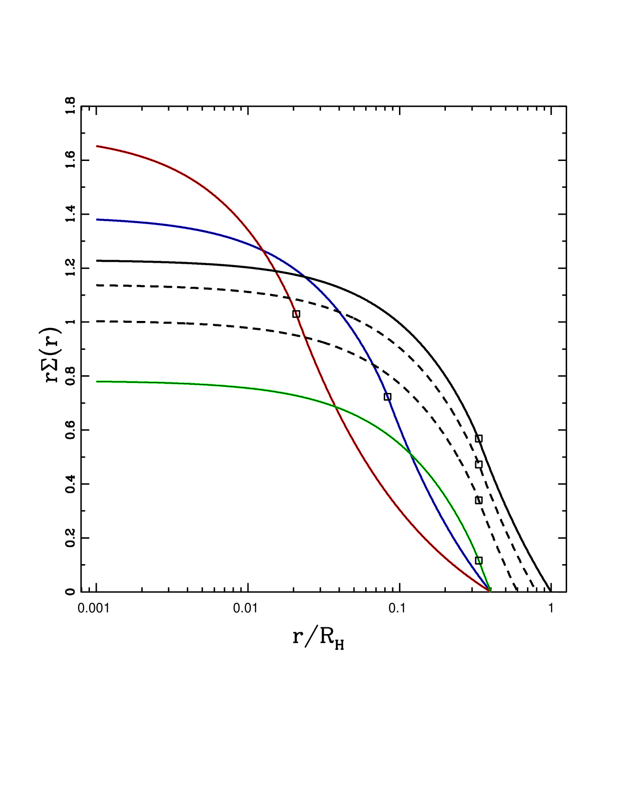
Figure 4: Surface density distributions for the circumplanetary disk for varying values of angular momentum bias factor $\lambda$ and outer disk boundary parameter $\xi$. The three colored curves show the surface density as a function of $r/R_{H}$ with a fixed outer boundary given by $\xi$ =2/5 and angular momentum bias factors $\lambda$ = 1 (green), 1/2 (blue), and 1/4 (red). The solid black curves shows the surface density for $\lambda$ = 1 and $\xi$ = 1. The dashed black curves correspond to $\lambda$ = 1 and $\xi$ = 0.8 (upper) and 0.6 (lower). The square symbols mark the location of the centrifugal radius $R_{C}/R_{H}=\lambda^{2}/3$.

4.7 Circumplanetary Disk Mass

The mass of the circumplanetary disk is given by integrating the surface density over the disk area, i.e.,

$$M_{\rm disk}=\int_{0}^{R_{H}}2\pi rdr\Sigma(r)={{\dot{M}}R_{C}^{2}\over 3\nu_{C}}\int_{0}^{u_{\rm out}}s_{k}(u)du\equiv{{\do tM}R_{C}^{2}\over 3\nu_{C}}I\,,$$ (83)

where the final equality defines the dimensionless integral $I$. We can integrate the profiles from the previous subsection to obtain

$$I={4\over 5}\left(1+\sqrt{u_{\rm out}}\right)-{3\pi\over 8}\,,\qquad\sqrt{u_{\rm out}}-{3\over 5}\,,\qquad{4\over 3}\left(1+\sqrt{u_{\rm out}}\right)-{3\pi\over 4}\,,$$ (84)

$${3\over 2}\left(1+\sqrt{u_{\rm out}}\right)-{128\over 15\pi}\,,\qquad{\rm and}\qquad{8\over 5}\left(1+\sqrt{u_{\rm out}}\right)-{15\pi\over 16}\,.$$

The characteristic mass scale for the disks is given by the leading coefficient, which can be evaluated for typical parameters to obtain

$$M_{\ast}\equiv{{\dot{M}}R_{C}^{2}\over 3\nu_{C}}\approx 3.9\times 10^{-4}\,M_{\rm Jup}\,\left({\alpha\over 10^{-3}}\right)^{-1}\left({{\dot{M}}\over 1M_{\rm Jup}{\rm Myr}^{-1}}\right)\left({M\over 1M_{\rm Jup}}\right)^{2/3}\,,$$ (85)

where we have assumed that the planet resides at $a=5$ AU, the stellar mass $M_{\ast}=1M_{\odot}$, and the angular momentum bias $\lambda=\sqrt{6}/6$. For completeness, the corresponding surface density for a disk in steady-state accretion is determined by the leading coefficient

$$\Sigma_{\ast}\equiv{{\dot{M}}\over 6\pi\nu_{C}}\approx 1400\,{\rm g}\,{\rm cm}^{-2}\left({\alpha\over 10^{-3}}\right)^{-1}\left({{\dot{M}}\over 1M_{\rm Jup}{\rm Myr}^{-1}}\right)\,.$$ (86)

It is instructive to compare these values with the properties of circumstellar disks that provide the planet forming environment. Circumplanetary disks are expected to have much lower masses in steady-state, $M_{\rm d}\sim 0.001M_{\rm Jup}$ compared to $\sim 50M_{\rm Jup}$ for the Minimum Mass Solar Nebula (MMSN; e.g., Hayashi 1981). On the other hand, the surface densities are comparable: The MMSN has $\Sigma\sim 1000$ g cm^-2 at 1 AU.

4.8 Disk Temperature Distributions

The above analysis determines the mass accretion rate through the disk and the corresponding surfaces density profiles. These solutions, in turn, determine the temperature distribution of the circumplanetary disk due to accretion. The energy dissipated per unit time per unit energy is given by

$$D(r)=\nu\Sigma\left(r{d\Omega\over dr}\right)^{2}={9\over 4}\nu\Sigma{GM\over r^{3}}\,,$$ (87)

where the final equality holds for a Keplerian rotation curve (as expected here). If the disk is sufficiently optically thick, it develops a photosphere with a well defined temperature, and radiates like a blackbody to leading order. Using the surface density distributions of this paper, specifically the form of equation (77), the disk temperature is given by

$$\sigma T^{4}={3\over 8\pi}{GM{\dot{M}}_{\rm in}\over r^{3}}s_{k}(u)\,,$$ (88)

where $u=r/R_{C}$. As a result, the temperature departs from the familiar form $T\sim r^{-3/4}$ by a factor of $[s_{k}(u)]^{1/4}$. This correction factor approaches a constant of order unity in the inner limit $u\ll 1$, and tapers off so that the temperature vanishes in the limit $u\to u_{\rm out}$ (where $s_{k}\to 0$). Note that the quantity ${\dot{M}}_{\rm in}$ is the total rate at which the planet/disk system gathers fall from the infalling envelope. Only a fraction $\gamma_{\rm in}$ of this mass is accreted by the planet, with the remainder transfered outward to conserve angular momentum. The required efficiency factor is included in the specification of the functions $s_{k}(u)$.

Note that the temperature given by equation (88) represents the contribution provided by disk accretion only. In addition, the material falling onto the disk will dissipate some of its energy in a shock on the disk surface (Adams & Shu, 1986; Adams & Batygin, 2022) and will dissipate additional energy as it adjusts to the the pre-existing Keplerian rotation profile (Cassen & Moosman 1981; Section 3). Radiation from both the central planet and the background circumstellar disk provide additional contributions to the heating of the surface of the circumplanetary disk. As a result, the effective surface temperature of the disk will be hotter than that given by equation (88).

5 Conclusion

This paper considers the formation of circumplanetary disks that form alongside their host planets during the late stages of giant planet formation. Due to conservation of angular momentum, most of the mass that eventually accretes onto the forming planet is processed through the disk. These disk structures are crucial for transporting angular momentum outward, so that mass can be be transferred onto the planet.

5.1 Summary of Results

This paper generalizes previous calculations in several ways: [a] We include the angular momentum bias $\lambda$, which accounts for the fact that the incoming material – at the outer boundary of the Hill sphere – does not necessarily have the same rotation rate as the mean motion of the planet. The bias factor is expected to lie in range $\lambda\approx 1/3-1/2$ during the late stages of formation (see Ward & Canup 2010 and references therein). [b] We generalize the orbit solutions that describe the trajectories of incoming material (see Section 2 and Mendoza et al. 2009) starting at the Hill sphere and eventually falling onto the surface of the circumplanetary disk. [c] We modify the outer boundary of the circumplanetary disk. Instead of extending all the way out to the Hill radius, the disk will be effectively truncated at a smaller distance $R_{\rm out}$ due to orbit crossing. As a result, we enforce the outer boundary conditions at $\xi=R_{\rm out}/R_{H}\approx 0.41$ (Martin & Lubow, 2011). [d] Finally, we account for the redistribution of incoming material after it falls onto the circumplanetary disk. The newly added material does not, in general, have the angular momentum appropriate for a Keplerian orbit around the planet at the location where it joins the disk (Cassen & Moosman, 1981; Cassen & Summers, 1983). As a result, new material mixes with pre-existing disk gas and dissipates energy while conserving angular momentum. This readjustment changes the form of the source term for material being added to the disk (equation [40]). The effects of angular momentum adjustment on the surface densities are outlined in Appendix C.

Including the aforementioned generalizations, we have constructed analytic solutions (Section 4) for the disk surface density distribution $\Sigma(r)$ for a range of infall geometries (as characterized by the geometrical functions $f(u)$; see equation [53]). The resulting surface density profiles have the approximate form $\nu\Sigma\to$ constant in the inner limit $r\to 0$, and smoothly decrease beyond the centrifugal barrier so that $\Sigma\to 0$ at the outer disk edge (see Figures 2 and 3). For expected parameters, the viscosity $\nu\propto{r}$ so that $\Sigma\sim 1/r$ over most of the disk within the centrifugal radius. Note that the functional forms for the surface density distributions are relatively insensitive to the angular distribution of the incoming material (set by $f[u]$) and have the same general form as found previously.

Although the general form for the surface density profiles $\Sigma(u)$ are robust, the generalizations of this paper lead to important corrections (see Figure 4). The inclusion of the angular momentum bias reduces the size of the centrifugal barrier $R_{C}$ by a factor of $\lambda^{2}\sim 1/9-1/4$ (for expected values $\lambda=1/3-1/2$). For the benchmark case of a 1 $M_{\rm Jup}$ planet forming at $a$ = 5 AU, we find $R_{C}\approx 3\times 10^{11}$ cm $\approx$ 30 $R_{P}$. In terms of the present-day Jovian satellite system, this estimate for the centrifugal barrier lies outside the orbit of Callisto and inside the orbit of the irregular moon Themisto. In addition to resulting in smaller disks, the smaller values for $R_{C}$ lead to larger values for the column density of the infalling envelope surrounding the planet. The column density scales as $N_{\rm col}\propto R_{C}^{-1/2}$ $\propto\lambda^{-1}$ (Adams & Shu, 1986; Adams & Batygin, 2022).

In general, accretion disks have inward flow in the inner limit and outward flow at their outer boundary. The radius $u_{0}$ where the mass accretion rate vanishes (so that ${\dot{M}}$ changes sign) plays an important role in determining disk structure, and has important implications for the formation of Jovian moons (Canup & Ward, 2002; Batygin & Morbidelli, 2020). Although the geometric distribution of incoming material has only a modest effect on the general form of the suface density, the values of $u_{0}$ depend on the choice of $f(u)$. For the five cases considered here, the we find $u_{0}$ = 0.350, 0.482, 0.751, 0.800, and 0.832 for $k=1-5$ (polar to isotropic to equatorial concentrations). The physical radius where the accretion flow changes sign is given by $R_{0}=u_{0}R_{C}=u_{0}\lambda^{2}R_{H}/3$.

In these systems, the circumplanetary disk initially accretes the majority of the mass and angular momentum impinging upon the central object. Since the planet itself carries little angular momentum, relative to the total incoming amount (even if the planet spins at breakup), the disk must transfer essentially all of the angular momentum outward to the outer disk boundary, where it joins the reservoir of the background circumstellar disk. Conservation of angular momentum necessarily results in some loss of mass, so that the accretion process cannot be fully efficient. The accretion efficiency is determined by the fraction of the infalling material that accretes onto the central planet (see Section 4), and can be written in the form

$$\gamma_{\rm in}=1-{{\cal F}_{k}\lambda\over\sqrt{3\xi}}\,,$$ (89)

where ${\cal F}_{k}$ is the dimensionless angular momentum for a given infall geometry (labeled by the index $k$; see equation [54]), $\lambda$ is the angular momentum bias, and $\xi$ defines the outer boundary of the disk $R_{\rm out}$ = $\xi R_{H}$. For expected values of the parameters, the efficiency lies in the range $\gamma_{\rm in}\approx$ 0.64 – 0.82. Since $\lambda^{2}<\xi$, inclusion of both the angular momentum bias and corrections to the outer disk boundary result in a higher efficiency compared to previous treatments.

5.2 Discussion

The results of this paper define length scales that characterize the properties and drive the evolution of circumplanetary disks. In addition to the planetary radius $R_{P}$, previous work has defined the magnetic truncation radius $R_{X}$ (Ghosh & Lamb, 1978; Blandford & Payne, 1982), the centrifugal radius (Ulrich, 1976; Quillen & Trilling, 1998), and invoked the Hill radius $R_{H}$ as the boundary for the planetary sphere of influence. In addition, this work sets the outer disk boundary $R_{\rm out}$ at a fraction of the Hill radius, determines the radii $R_{0}$ where the mass accretion flow changes sign, and makes the distinction between the centrifugal radius and the initial disk radius $R_{\rm d}$ (which depends on the starting radial velocity – see equation [18]). These length scales obey the ordering

$$R_{P}<R_{X}<R_{0}<R_{\rm d}\,\raise 1.29167pt\hbox{$<$}\kern-7.5pt\lower 3.01385pt\hbox{$\sim$}\,R_{C}<R_{\rm out}<R_{H}\,.$$ (90)

This paper has generalized the approach used in previous work regarding the starting conditions at the Hill sphere, the outer disk boundary, and manner in which incoming material enters the disk. Like any analytical treatment, this paper makes approximations, including that of azimuthal symmetry, neglect of magnetic fields, and the use of ballistic trajectories (see Adams & Batygin 2022 for a more detailed discussion of their validity). On this latter issue, we note that the infalling envelope must be able to cool sufficiently in order for the circumplanetary disk to form. This cooling requirement implies an upper limit to the mass infall rate ${\dot{M}}_{\rm in}$. More specifically, successful disk formation requires the cooling time of the envelope to be shorter than the free-fall time – analogous to classic arguments regarding opacity limited fragmentation (see Rees 1976). This constraint, derived in Appendix A, implies the upper bound ${\dot{M}}_{\rm in}\,\raise 1.29167pt\hbox{$<$}\kern-7.5pt\lower 3.01385pt\hbox{$\sim$}\,70$ $M_{\rm Jup}$ Myr^-1. The other key assumption is that the circumplanetary disk can reach steady-state, which requires the viscous evolution time $t_{\nu}=R_{C}^{2}/\nu$ to be shorter than the infall time scale $t_{\rm in}=M/{\dot{M}}_{\rm in}$, a constraint that is readily met (see Section 4).

The surface density profiles found in this paper apply to late stages of the core accretion paradigm for planet formation, when the growing planet accumulates the majority of its mass. During this time, the Hill radius is smaller than the Bondi radius, but the planet remains (at least mostly) embedded within its parental circumstellar disk. At still later times, however, the Hill radius can exceed the scale height of the circumstellar disk and the planet can clear a gap in the nebula. Both of these circumstances act to reduce the amount of gas flowing into the Hill sphere, eventually leading to a decrease in ${\dot{M}}_{\rm in}$, so that we expect most of the planetary mass to be accreted beforehand. Nonetheless, these final stages are important for determining the final mass of the planet and for the issues related to satellite formation. As such, these end stages should be considered in future work.

We are grateful to A. Taylor for useful discussions. This work was supported by the University of Michigan, the California Institute of Technology, the Leinweber Center for Theoretical Physics, and by the David the Lucile Packard Foundation.

Appendix A Cooling Constraint

As outlined in Section 1, numerical simulations show that the formation of circumplanetary disks requires sufficient cooling. Recent multi-fluid simulations (Krapp et al., 2024) indicate that the gas must cool on a timescale at least ten times shorter than the orbital timescale in order to retain high angular momentum and form a disk. If the cooling time is longer (cooling is inefficient), the outcome is an isentropic, convective envelope that extends through much of the Hill sphere and rotates far below the Keplerian speed. In essence, rapid cooling allows the inflow to become rotationally supported, whereas slow cooling leads to adiabatic compression that thermally ‘inflates’ the gas, wiping out any nascent disk. This thermodynamic criterion thus sets a high bar for circumplanetary disk formation. To understand the origin of this criterion, this Appendix finds the conditions required for the cooling time of the infalling envelope to be shorter than the free-fall time. This condition, $t_{\rm cool}<t_{\rm ff}$, is required for disk formation and can also be used to place a limit on the infall rate.

The cooling time for the envelope can be written in the form

$$t_{\rm cool}={{\cal U}_{\rm env}\over 4\pi r^{2}\sigma T^{4}}\,\tau_{\rm eff}\,,$$ (A1)

where ${\cal U}_{\rm env}$ is the thermal energy of the infalling envelope, i.e., the energy that must be radiated away in order for the flow to continue. The scale $r$ is some characteristiec radius. The effective optical depth $\tau_{\rm eff}$ can be written in terms of the actual optical depth $\tau$ (Rees, 1976) according to the relation

$$\tau_{\rm eff}={1\over 2}\left(\tau+{1\over\tau}\right)\,.$$ (A2)

The free fall time can be written in the form

$$t_{\rm ff}={\sqrt{2}\over 3}\left({GM\over R^{3}}\right)^{-1/2}\,,$$ (A3)

where $R$ is radius where effective cooling is enforced. In order for disk formation to take place, this radius must be comparable to the disk size so that $R=R_{C}$. At this radius, the free-fall time from equation (A3) is about an order of magnitude shorter than the orbit time of the forming planet (so that the requirement $t_{\rm cool}<t_{\rm ff}(R_{C})$ is consistent with that advocated by Krapp et al. 2024 based on numerical simulations). To evaluate the thermal energy of the infalling envelope, we find the energy that would be present if the gas heats up adiabatically according to $P\propto\rho^{5/3}$ so that $v_{s}^{2}\propto$ $T\propto\rho^{2/3}$. We then integrate over the envelope using the density distribution for the infall to find

$${\cal U}_{\rm env}=\int_{0}^{R_{H}}4\pi r^{2}dr\rho v_{sH}^{2}(\rho/\rho_{H})^{2/3}=8\pi CR_{H}^{3/2}v_{s}^{2}={\sqrt{2}{\dot{M}}_{\rm in}R_{H}^{3/2}\over\sqrt{GM}}v_{s}^{2}(R_{H})\,,$$ (A4)

where the sound speed $v_{s}$ is evaluated at the Hill radius. After combining these results, the cooling constraint takes the form

$$4\pi r^{2}\sigma T^{4}>{\dot{M}}_{\rm in}3v_{s}^{2}\left({R_{H}\over R_{C}}\right)^{3/2}\tau_{\rm eff}\,.$$ (A5)

The left-hand-side of the equation is determined by the envelope luminosity, which must be a fraction of the total system luminosity, so that

$$4\pi r^{2}\sigma T^{4}=\beta{GM{\dot{M}}_{\rm in}\over R_{P}}\left[1-\exp(-\tau_{\ast})\right]\,.$$ (A6)

This expression assumes that the total luminosity is given by the incoming material falling to the planetary surface. The envelope must radiate a fraction of this total power as determined by the optical depth $\tau_{\ast}$ of the envelope to the radiation from the central source. Note that this optical depth $\tau_{\ast}$ is generally larger than the optical depth $\tau$ of the envelope to its internally emitted radiation. The dimensionless parameter $\beta\,\raise 1.29167pt\hbox{$<$}\kern-7.5pt\lower 3.01385pt\hbox{$\sim$}\,1$, where the maximum value corresponds to maximally efficient accretion, with all of the gas falling to the planetary surface and no energy stored in rotation. Using the expression (A6) for luminosity in the cooling constraint, we find

$$\Lambda\left[1-{\rm e}^{-\tau_{\ast}}\right]>\tau+{1\over\tau}\,,$$ (A7)

where the dimensionless parameter $\Lambda$ is defined by

$$\Lambda\equiv\beta{2GM\over 3v_{s}^{2}R_{P}}\left({R_{C}\over R_{H}}\right)^{3/2}\approx 20\beta\left({T_{H}\over 134\,{\rm K}}\right)^{-1}\left(\sqrt{6}\lambda\right)^{3}\,.$$ (A8)

For much of the parameter space of interest, the optical depth of the central source radiation is large enough that we can ignore the decaying exponential $\exp[-\tau_{\ast}]$, so the constraint simplifies to the form

$$\tau\,\raise 1.29167pt\hbox{$<$}\kern-7.5pt\lower 3.01385pt\hbox{$\sim$}\,\Lambda\approx 20\qquad{\rm where}\qquad\tau\approx 0.3\left({{\dot{M}}_{\rm in}\over 1M_{\rm Jup}/{\rm Myr}}\right)\left({M\over 1M_{\rm Jup}}\right)^{-2/3}\,.$$ (A9)

The corresponding constraint on the mass infall rate becomes

$${\dot{M}}_{\rm in}\,\raise 1.29167pt\hbox{$<$}\kern-7.5pt\lower 3.01385pt\hbox{$\sim$}\,70\,M_{\rm Jup}\,{\rm Myr}^{-1}\,\left({M\over 1M_{\rm Jup}}\right)^{2/3}\,.$$ (A10)

Note that we have some flexibility in choosing numbers to evaluate the constraint, so a more conservative limit would be ${\dot{M}}_{\rm in}\,\raise 1.29167pt\hbox{$<$}\kern-7.5pt\lower 3.01385pt\hbox{$\sim$}\,100$ $M_{\rm Jup}$/Myr. In any case, the infall rate cannot become arbitarily large and still allow for the envelope to cool, form a disk, and effectively transfer material onto the planet.

Appendix B Simple Fitting Functions

Although this paper has successfully obtained analytic forms for the surface density profiles of circumplanetary disks, the resulting forms are somewhat complicated (see Section 4). On one hand, these complicated functions are necessary for the surface density profiles to follow the angular momentum budget for a given source function. On the other hand, simpler but more approximate forms are useful in some applications. The surface density profiles for the five geometries of interest can be written in the form

$$\Sigma=\Sigma_{0}\,u^{-1}\exp[-u/2u_{0}]\,,$$ (B1)

where $u=r/R_{C}$, $u_{0}$ is the location in the disk where the mass accretion rate through the disk changes sign, and the leading constant is given by

$$\Sigma_{0}={{\dot{M}}_{\rm in}\over 3\pi\nu_{C}}\left[1-{{\cal F}_{k}\over\sqrt{u_{\rm out}}}\right]\,,$$ (B2)

where the angular momentum factors ${\cal F}_{k}$ for the five cases of interest are given by equation (54) and where $u_{\rm out}=R_{\rm out}/R_{C}=3\xi/\lambda^{2}$. Note that all of the constants in the expression are determined by the properties of the full analytic solutions. With these specifications, by construction, the surface density has the (exact) correct form in the limit $u\to 0$ and the corresponding mass accretion rate changes sign at the proper location. The largest departure of the fitting formula from the exact solutions occurs near the outer disk edge where $\Sigma(u_{\rm out})\to 0$. The resulting fits are thus approximate. If we define the root-mean-square errors according to

$${\cal E}_{k}\equiv\left[\int_{0}^{u_{\rm out}}(s_{k}-s_{k{\rm fit}})^{2}du\right]^{1/2}\left[\int_{0}^{u_{\rm out}}s_{k}du\right]^{-1},$$ (B3)

then the errors ${\cal E}_{k}$ $\approx$ 0.11, 0.058, 0.030, 0.070, and 0.095 for the five cases shown in Figure 3. For the infall profiles concentrated along the equator ($k=4,5$), the fitting functions perform poorly for radii beyond the centrifugal barrier ($u>1$); the errors are not overly large because the profiles decrease rapidly in this regime. One can readily find more accurate fitting formulae – but at the expense of needing more complicated expressions.

As one example of the utility of these fitting functions, the total disk accretion luminosity can be written in the form

$$L_{\rm ac}={3GM{\dot{M}}_{\rm in}\over 2R_{X}}\int_{1}^{\infty}{d\xi\over\xi^{2}}\exp[-q\xi]={3GM{\dot{M}}_{\rm in}\over 2R_{X}}{\rm E}_{2}(q)\,,$$ (B4)

where $q=R_{X}/(2u_{0}R_{C})$ and $E_{2}$ is the exponential integral (Abramowitz & Stegun, 1972). Recall that the disk is truncated on the inside at $R_{X}$ due to magnetic fields from the planet.

Appendix C Effect of Angular Momentum Adjustment on the Surface Density

This Appendix compares the surface density solutions of this paper with those found earlier without angular momentum adjustment. In addition to angular momentum bias and modified outer boundary conditions, this paper explicitly includes the redistribution of incoming material as it impacts the circumplanetary disk. The original source term from equation (40) specifies the rate at which the surface of the disk gains mass. Since the incoming material does not have the proper angular momentum, that appropriate for a Keplerian rotation curve, it adjusts its position accordingly (see Section 3). Due to this adjustment, the effective source term is modified, as shown by the first term in the surface density evolution equation (55). In order to isolate the effects of angular momentum adjustment on the resulting surface density profiles, we determine the analogs of the functions $s_{k}(u)$ from Section 4.6. Here we use equation (40) as the source term, without angular momentum adjustment, so that the disk evolution equation simplifies to the form

$${\cal S}(u)+{3\over R_{C}^{2}}{1\over u}{\partial\over\partial u}\left(\sqrt{u}{\partial\over\partial u}\left[\sqrt{u}\nu\Sigma\right]\right)=0\,,$$ (C1)

where the source term includes the geometric function $f_{k}(u)$ for the different infall geometries. We use the same angular momentum bias and disk outer boundary as before, so that $u_{\rm out}=5$. The resulting forms for the surface density profiles are those given by equations (41–46) from Taylor & Adams (2024), except that these earlier solutions were expressed in terms of arbitrary constants $K_{1}$ and $K_{2}$ (see also Adams & Batygin 2022). Here we specify the constants to meet the aforementioned boundary conditions and to be consistent with the solutions from the present paper.

The resulting surface density profiles, both with and without angular momentum adjustment, are presented in Figure 5. In the upper panel, the solid curves show the surface density profiles $s_{k}(u)$ from this paper (the same as in Figure 3). The five solutions for the different infall geometries are shown in blue ($k=1$), cyan ($k=2$), green ($k=3$), magenta ($k=4$), and red ($k=5$), from top to bottom on the left side of the plot. The corresponding surface density profiles, calculated without angular momentum adjustment, are shown as the dashed curves (with the same ordering and colors). The bottom panel of Figure 5 shows the ratio of the surface density profiles for the five infall geometries. These results show that the inclusion of angular momentum adjustment makes the surface density relatively higher at small radii and correspondingly smaller at larger radii. In other words, the surface density profiles become steeper. This trend is expected, as the adjustment process (Section 3) acts to move incoming material inward. The magnitude of the effect is modest, however, as shown in the lower panel. Over most of the radial range of interest, the difference is of order 10 – 20%.

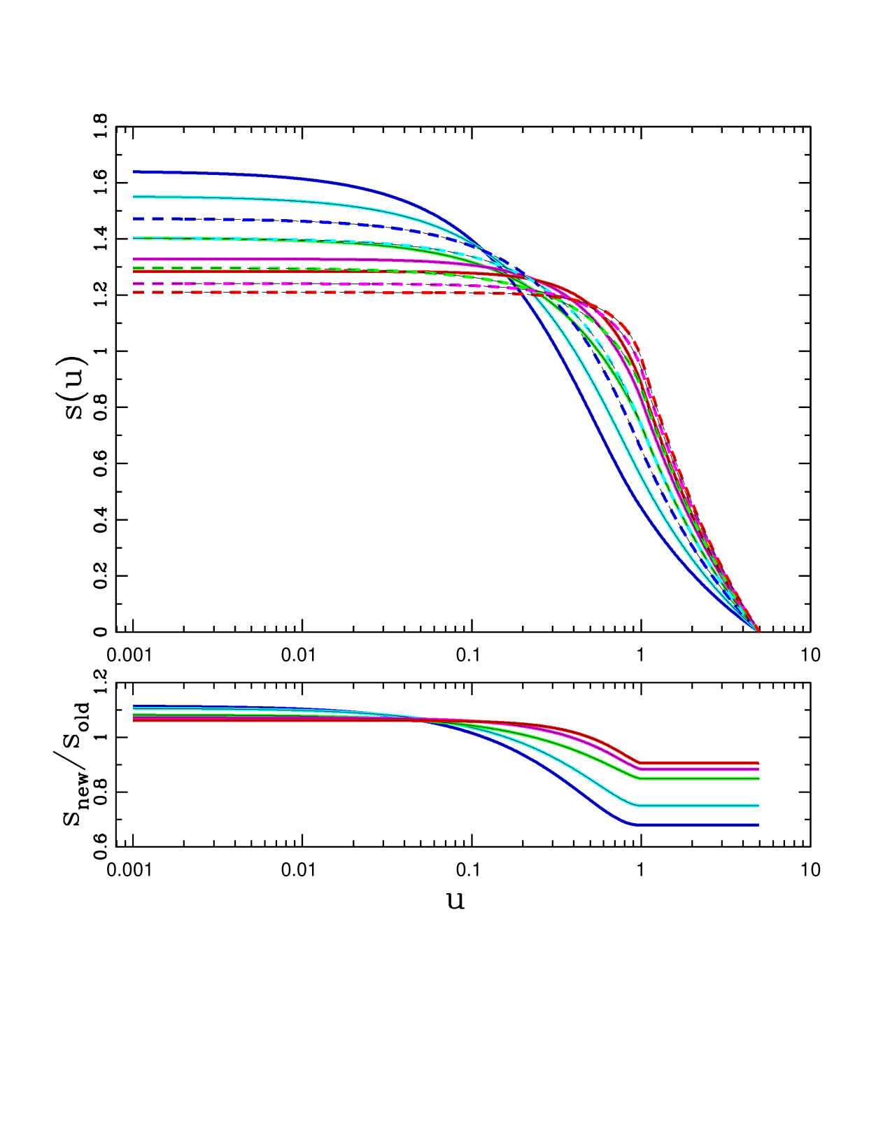
Figure 5: Surface density distributions for the circumplanetary disks with and without angular momentum adjustment (see text). In the upper panel, solid curves show the solutions with angular momentum adjustment, for polar flow ($k=1$, solid blue) to isotropic ($k=3$, solid green), to equatorial ($k=5$, solid red). The dashed curves show the corresponding sufface density profiles calculated in the absence of angular momentum adjustment. The lower panel shows the ratio of the profiles with adjustment ($s_{\rm new}$) to those without ($s_{\rm old}$), where the index runs from $k=1$ (upper blue on the left) to $k=5$ (lower red on the left).

References

- Abramowitz & Stegun (1972) Abramowitz, M., & Stegun, I. A. 1972, Handbook of Mathematical Functions (New York: Dover)
- Adams & Batygin (2022) Adams, F. C., & Batygin, K. 2002, ApJ, 934, 111
- Adams & Shu (1986) Adams, F. C., & Shu, F. H. 1986, ApJ, 308, 836
- Ayliffe & Bate (2009) Ayliffe, B. A., & Bate, M. R. 2009, MNRAS, 397, 657
- Bae et al. (2022) Bae, J., Teague, R., Andrews, S. M., et al. 2022, ApJL, 934, L20
- Bailey et al. (2023) Bailey, A. P., & Zhu, Z. 2024, MNRAS, 534, 2953
- Batygin & Morbidelli (2020) Batygin, K., & Morbidelli, A. 2020, ApJ, 894, 143
- Benisty et al. (2021) Benisty M., Bae, J., Facchini, S., et al., 2021, ApJ, 916, L2
- Blandford & Payne (1982) Blandford, R. D., & Payne, D. G. 1982, MNRAS, 199, 883
- Bodenheimer & Pollack (1986) Bodenheimer, P., & Pollack, J. B. 1986, Icarus, 67, 391
- Canup & Ward (2002) Canup, R. M., & Ward, W. R. 2002, AJ, 124, 3404
- Cassen & Moosman (1981) Cassen, P., & Moosman, A. 1981, Icarus, 48, 353
- Cassen & Summers (1983) Cassen, P., & Summers, A. 1983, Icarus, 53, 26
- Chevalier (1983) Chevalier, R. 1983, ApJ, 268, 753
- Choksi & Chiang (2025) Choksi, N., & Chiang, E. 2025, MNRAS, 537, 2945
- Christiaens et al. (2024) Christiaens, V., Samland, M., Henning, T., et al. 2024, A&A, 685, L1
- Cugno et al. (2024) Cugno, G., Patapis, P., Banzatti, A., et al. 2024, ApJ, 966, L21
- Fung et al. (2019) Fung, J., Zhu, Z., & Chiang, E. 2019, ApJ, 887, 152
- Ghosh & Lamb (1978) Ghosh, P., & Lamb, F. K. 1978, ApJ, 223, L83
- Hartmann (2009) Hartmann, L. W. 2009, Accretion Processes in Star Formation (Cambridge: Cambridge Univ. Press)
- Hayashi (1981) Hayashi, C. 1981, PThPS, 70, 35
- Hernández et al. (2007) Hernández, J., Hartmann, L., Megeath, M. et al. 2007, ApJ, 662, 1067
- Hubickyj et al. (2005) Hubickyj, O., Bodenheimer, P., & Lissauer, J. J. 2005, Icarus, 179, 415
- Klahr & Kley (2006) Klahr, H., & Kley, W. 2006, A&A, 445, 747
- Krapp et al. (2024) Krapp, L., Kratter, K. M., Youdin, A. N. et al. 2024, ApJ, 973, 153
- Lambrechts & Lega (2017) Lambrechts, M., & Lega, E. 2017, A&A, 606, 146
- Lambrechts et al. (2019) Lambrechts, M., Lega, E., Nelson, R. P., Crida, A., & Morbidelli, A. 2019, A&A, 630, 82
- Lega et al. (2024) Lega, E., Benisty, M., Cridland, A., Morbidelli, A., Schulik, M., & Lambrechts, M. 2024, A&A, 690, 183
- Lesur et al. (2023) Lesur, G., Flock, M., Ercolano, B., et al. 2023, in ASP Conf. Ser. 534, Protostars and Planets VII, ed. S. Inutsuka et al. (San Francisco, CA: ASP), 465
- Lissauer & Kary (1991) Lissauer, J. J., & Kary, D. M. 1991, Icarus, 94, 126
- Machida et al. (2008) Machida, M. N., Kokubo, E., Inutsuka, S., & Matsumoto, T. 2008, ApJ, 685, 1220
- Martin & Lubow (2011) Martin R. G., & Lubow S. H. 2011, MNRAS, 413, 1447
- Mendoza et al. (2009) Mendoza, S., Tejeda, E., & Nagel, E. 2009, MNRAS, 393, 579
- Quillen & Trilling (1998) Quillen, A. C., & Trilling, D. E. 1998, ApJ, 508, 707
- Pollack et al. (1996) Pollack, J. B., Hubickyj, O., Bodenheimer, P., Lissauer, J. J., Podolak, M., & Greenzweig, Y. 1996, Icarus, 124, 62
- Rees (1976) Rees, M. J. 1976, MNRAS, 176, 483
- Schulik et al. (2020) Schulik, M., Johansen, A., Bitsch, B., Lega, E., & Lambrechts, M. 2020, A&A, 642, A187
- Shu (1990) Shu, F. H. 1990, Gas Dynamics: The physics of astrophysics (Mill Valley: Univ. Science Books)
- Szulágyi et al. (2016) Szulágyi, J., Masset, F., Lega, E., et al. 2016, MNRAS, 460, 2
- Szulágyi (2017) Szulágyi, J. 2017, ApJ, 842, 103
- Szulágyi & Mordasini (2017) Szulágyi, J., & Mordasini, C. 2017, MNRAS, 465, 64
- Szulágyi et al. (2019) Szulágyi, J. Dullemond, C. P., Pohl, A., & Quanz, S. P. 2019, MNRAS, 487, 1248
- Tanigawa et al. (2012) Tanigawa, T., Ohtsuku, K., & Machida, M. N. 2012, ApJ, 747, 47
- Tanigawa & Tanaka (2016) Tanigawa, T., & Tanaka, H. 2016, ApJ, 823, 48
- Taylor & Adams (2024) Taylor, A. G., & Adams, F. C. 2024, Icarus, 415, 116044
- Taylor & Adams (2025) Taylor, A. G., & Adams, F. C. 2025, Icarus, 425, 116327
- Terebey et al. (1984) Terebey, S., Shu, F. H., & Cassen, P. 1984, ApJ, 286, 529
- Ulrich (1976) Ulrich, R. K. 1976, ApJ, 210, 377
- Ward & Canup (2010) Ward, W. R., & Canup, R. M. 2010, ApJ, 140, 1168
- Zhu (2015) Zhu, Z. 2015, ApJ, 799, 16
- Zhu et al. (2018) Zhu, Z., Andrews, S. M., & Isella, A. 2018, MNRAS, 479, 1850
- Zhu et al. (2024) Zhu, Z., Stone, J. M., & Calvet, N. 2024, MNRAS, 528, 2883