A hybrid U-Net and Fourier neural operator framework for the fast prediction of turbulent flows with mixed periodic and non-periodic boundary conditions

Abstract

Accurate and efficient predictions of three-dimensional (3D) turbulent flows are of significant importance in the fields of science and engineering. In the current work, we propose a hybrid U-Net and Fourier neural operator (HUFNO) method, tailored for mixed periodic and non-periodic boundary conditions which are often encountered in complex turbulence problems. The HUFNO model is tested in the large-eddy simulation (LES) of 3D periodic hill turbulence featuring strong flow separations. Compared to the original Fourier neural operator (FNO) and the convolutional neural network (CNN)-based U-Net framework, the HUFNO model has a higher accuracy in the predictions of the velocity field and Reynolds stresses. Further numerical experiments in the LES show that the HUFNO framework outperforms the traditional Smagorinsky (SMAG) model and the wall-adapted local eddy-viscosity (WALE) model in the predictions of the turbulence statistics, the energy spectrum, the wall stresses and the flow separation structures, with much lower computational cost. Importantly, the accuracy and efficiency are transferable to unseen initial conditions and hill shapes, underscoring its great potentials for the fast prediction of strongly separated turbulent flows over curved boundaries.

[1]organization=Department of Mechanics and Aerospace Engineering, Southern University of Science and Technology, city=Shenzhen, postcode=518055, country=China [2]organization=Guangdong Provincial Key Laboratory of Turbulence Research and Applications, Southern University of Science and Technology, city=Shenzhen, postcode=518055, country=China [3]organization=Harbin Engineering University Qingdao Innovation and Development Base, city=Qingdao, postcode=266000, country=China [4]organization=Department of Biomedical Engineering, National University of Singapore, city=Singapore, postcode=117583, country=Singapore [5]organization=Department of Energy and Power Engineering, Nanchang Hangkong University, city=Nanchang, postcode=330063, country=China

An integrated framework of convolutional neural networks and Fourier neural operators, tailored for problems involving mixed periodic and non-periodic boundary conditions.

Machine learning-based surrogate model for the large-eddy simulation of three-dimensional turbulent flows over curved boundaries with strong flow separation.

High-accuracy stable data-driven approach for the fast prediction of long-term dynamics of periodic-hill turbulence, with transferable accuracy to unseen initial conditions and hill shapes.

1 Introduction

Turbulent flows are prevalent in the fields of aerospace engineering, air pollution control, meteorology and industrial processes, etc [1]. Among various flow prediction techniques, computational fluid dynamics (CFD) constitutes a critical tool, offering valuable insights into flow field information, particularly when experimental data are difficult to obtain [2]. Nevertheless, due to the vast range of motion scales involved, direct numerical simulation (DNS) of turbulent flows at high Reynolds numbers remains computationally prohibitive [3, 5, 4]. As such, coarse-grained simulations are often employed as reduced-order methods, such as the Reynolds-averaged Navier-Stokes (RANS) approach and large-eddy simulation (LES). While the RANS approach focuses on solving the mean flow field and has been widely utilized in industrial applications [8, 9, 6, 7, 12, 10, 11], the LES directly resolves the large-scale energy-containing motions, enabling more accurate predictions of the large-scale flow structures particularly for separated turbulence [16, 17, 13, 14, 15, 18, 19, 20, 21, 22]. However, LES incurs higher computational costs compared to RANS [16, 5].

While traditional flow simulation methods continue to develop, machine learning (ML)-based techniques for flow prediction have been widely proposed over the past decade, thanks to the rapid advancement of modern computing power and the accumulation of high-fidelity data [23, 25, 26, 24, 27, 28]. These efforts encompass a broad range of applications, including learning key aerodynamic forces in aerodynamic flow fields, such as the drag and lift coefficients [29, 30, 31], modeling parts of the governing equations such as the Reynolds stresses in RANS and the subgrid-scale (SGS) terms in LES [33, 34, 32, 35, 36, 37, 43, 42, 44, 46, 39, 40, 41, 38, 45, 47, 48], reconstructing wall models [49, 50], inferring missing information due to measurement constraints or flow field damage [52, 53, 51, 54], super-resolution of coarse-grained flow field [55, 56], and directly learning the temporal evolution of flow fields [59, 57, 58, 60, 61, 64, 65, 66, 63, 67, 68, 62, 69, 70, 71, 72, 73], etc. In these applications, directly simulating the flow field evolution has received increasing attention recently, considering that trained models can provide rapid evaluations of detailed flow information without having to solve the Navier-Stokes equations.

In the field of ML-based flow predictions, commonly adopted methods include the physics-informed neural networks (PINN)-based approaches [74, 75, 76, 78, 77], the recursive neural networks (RNN) and long short-term memory (LSTM)-based frameworks [64, 65, 79, 80, 81, 66, 63], and neural operator-based techniques [59, 57, 83, 60, 61]. For instance, Raissi et al. proposed a PINN-based framework to solve general nonlinear partial differential equations [74]. Wang et al. proposed a turbulent flow network (TF-Net) based on a specialized U-Net architecture incorporating physical constraints in the context of two-dimensional (2D) Rayleigh-Bénard (RB) convection [75]. Bukka et al. integrated proper orthogonal decomposition (POD) with deep learning (DL) to simulate the flow past a cylinder [63]. Han et al. conducted a series of studies using CNN and LSTM-based frameworks to predict flow field evolution and fluid-solid interaction [79, 80, 81].

Although many neural networks (NNs) are capable of effectively approximating mappings between finite-dimensional Euclidean spaces for specific datasets, they often struggle to generalize across different flow conditions or boundary configurations [74, 57]. To address this limitation, Li et al. introduced an innovative Fourier neural operator (FNO) framework, which efficiently learns mappings between high-dimensional features in Fourier space, enabling the reconstruction of information in infinite-dimensional spaces [57]. In their numerical tests, the proposed FNO model demonstrated remarkable accuracy in predicting two-dimensional (2D) turbulent flows. Following Li et al.’s work, numerous extensions and applications of FNO have been developed [82, 83, 58, 87, 90, 60, 61, 89, 59, 92, 84, 85, 91, 86, 88, 93, 96, 94, 95]. For instance, Tran et al. proposed a factorized version of the FNO framework to enhance the efficiency of the FNO framework [82]. To enhance the accuracy of FNO in predicting 2D turbulence at high Reynolds numbers, Peng et al. incorporated an attention mechanism into the FNO framework, leading to improved statistical predictions and instantaneous flow structures [60]. You et al. developed an implicit Fourier neural operator (IFNO) [88], which significantly reduced the number of trainable parameters and memory requirements compared to the original FNO. Wen et al. proposed a U-Net enhanced FNO (UFNO), which outperformed both the original FNO and CNN frameworks in solving complex gas-liquid multi-phase problems [89]. Lehmann et al. utilized FNO to predict the propagation of seismic waves [90]. Recently, Peng et al. further applied the FNO in real-time simulation of 3D dynamic urban microclimate [91].

While many NN-based flow prediction methods have been proposed, most of these methods are developed for laminar flows or 2D turbulence problems. For 3D turbulence, the nonlinear interactions are fundamentally more complex than those in 2D turbulence, making its modeling significantly more challenging. The increased model complexity also leads to higher memory demands and a greater number of NN parameters [83]. Mohan et al. introduced two reduced-order models based on a convolutional generative adversarial network (C-GAN) and a compressed convolutional long-short-term memory (CC-LSTM) network in the context of 3D homogeneous isotropic turbulence [64, 65]. Peng et al. further advanced the FNO model by incorporating a linear attention mechanism, leading to improved accuracy and efficiency in the 3D homogeneous isotropic turbulence and turbulent mixing layers [61]. More recently, Li et al. trained FNO and implicit U-Net enhanced FNO (IUFNO) models using coarsened DNS data of 3D isotropic turbulence and turbulent mixing layers [83, 87]. Their models can be viewed as surrogate models for the LES of turbulent flows. In their approach, the resulting NN models can effectively predict the long-term dynamics of 3D turbulence with sufficient accuracy and stability [87]. Although these efforts have demonstrated their effectiveness, they have primarily been applied to unbounded turbulent flows. For wall-bounded flows, Nakamura et al. integrated a 3D CNN autoencoder (CNN-AE) with an LSTM network to predict 3D turbulent channel flow [66], and the predicted statistics aligned well with DNS results. Jin et al. developed Navier-Stokes flow nets (NSFnets) using the physics-informed neural network (PINN) framework [76]. Given the initial and boundary conditions of the subdomain, their PINN-based solutions can be obtained for small subdomains in the case of turbulent channel flow. Recently, by enforcing the solid-wall boundary conditions, Wang et al. extended the application of the IUFNO framework to the LES of 3D turbulent channel flows at friction Reynolds numbers ranging from 180 to 590, leading to better predictions compared to the traditional LES simulations [97].

It is important to note that these limited studies on wall-bounded turbulence have only considered simple boundaries. However, the solid boundaries in real-world scenarios are more complex and often curved, potentially giving rise to strong flow separations, which further increase the prediction difficulties. In this regard, we shall focus on the strongly separated turbulent flows in this work. Meanwhile, to account for the non-periodic boundary conditions often encountered in problems with complex geometries, we combine the convolutional neural network (CNN)-based U-Net framework and Fourier neural operator (FNO) in a hybrid approach, namely the hybrid U-Net and FNO (HUFNO) framework. Further, it should also be noted that simulating all scales of turbulence for wall-bounded 3D turbulence at moderately high Reynolds numbers remains challenging for NN-based approaches, due to the potentially enormous number of NN parameters and the risk of overfitting. Therefore, we constrain the scope of the numerical tests to the prediction of the large-scale energy-containing motions of turbulence, i.e., using the HUFNO model as a surrogate model for the large-eddy simulation (LES) of turbulence. To incorporate the effect of curved boundaries, we adopted the turbulent flows over periodic hills as the benchmark problem for the HUFNO model. To the best of our knowledge, this represents the first attempt to develop surrogate LES models for strongly separated 3D wall-bounded turbulence in the presence of curved boundaries. As will be shown, the proposed model demonstrates significant promise compared to traditional LES models.

The rest of the paper is organized as follows. The governing equations of incompressible turbulence and traditional LES are introduced in Section 2, followed by a brief discussion on the solution strategies for the LES equations and their respective advantages and shortcomings. The FNO and HUFNO frameworks are introduced in Section 3. In Section 4, the performances of the proposed HUFNO frameworks are evaluated in the simulations of periodic hill turbulence, and compared against the DNS benchmark and the traditional LES results. Finally, a brief conclusion of the paper and some future perspectives are given in Section 5.

2 Governing equations of turbulent flows and the large-eddy simulation

In this section, the governing equations of incompressible turbulence are introduced, followed by a brief description of the traditional large-eddy simulation (LES) and the corresponding subgrid-scale (SGS) models.

For incompressible turbulence, the governing equations for the evolution of mass and momentum are given by the three-dimensional (3D) Navier-Stokes (NS) equations, namely [98, 99]

$$\frac{\partial u_{i}}{\partial x_{i}}=0,$$ (1)

$$\frac{\partial u_{i}}{\partial t}+\frac{\partial u_{i}u_{j}}{\partial x_{j}}=-\frac{\partial p}{\partial x_{i}}+\nu\frac{\partial^{2}u_{i}}{\partial x_{j}\partial x_{j}}+\mathcal{F}_{i},$$ (2)

where $u_{i}$ is the $i$th velocity component, $\nu$ is the kinematic viscosity, $p$ is the pressure divided by the constant density $\rho$, and $\mathcal{F}_{i}$ accounts for any external forcing. Throughout this paper, the summation convention is used unless otherwise specified.

To date, solving the NS equations using fine-grid DNS is yet impractical at high Reynolds numbers due to large range of scales involved [1, 3, 5, 4]. Compared to DNS, LES only simulates the dominant large-scale energy-containing motions using a coarse grid, and the subgrid-scale effects are modeled as functions of the resolved scales. [16, 17, 18, 13, 14, 15]. By filtering the NS equations, the governing equations for LES can be obtained as [3, 16]

$$\frac{\partial\overline{u}_{i}}{\partial x_{i}}=0,$$ (3)

$$\frac{\partial\overline{u}_{i}}{\partial t}+\frac{\partial\overline{u}_{i}\overline{u}_{j}}{\partial x_{j}}=-\frac{\partial\overline{p}}{\partial x_{i}}-\frac{\partial\tau_{ij}}{\partial x_{j}}+\nu\frac{\partial^{2}\overline{u}_{i}}{\partial x_{j}\partial x_{j}}+\overline{\mathcal{F}}_{i},$$ (4)

with the overbar denoting a filtered variable, which is calculated as

$$\overline{f}(\mathbf{x})=\int_{D}f(\mathbf{x}-\mathbf{r})G(\mathbf{r},\mathbf{x};\overline{\Delta})d\mathbf{r},$$ (5)

where $f$ represents the physical quantity of flow field, here being velocity and pressure. G denotes the filter kernel, $\overline{\Delta}$ is the filter width and D represents the physical domain. The unclosed SGS stress $\tau_{ij}$ is given by

$$\tau_{ij}=\overline{u_{i}u_{j}}-\overline{u}_{i}\overline{u}_{j},$$ (6)

representing the nonlinear interactions between the resolved and SGS motions. Apparently, if the SGS stress can be modeled in terms of the resolved variables, the LES equations are closed.

In the LES community, a well-known SGS model is the Smagorinsky (SMAG) model [13], namely

$$\tau^{A}_{ij}=\tau_{ij}-\frac{\delta_{ij}}{3}\tau_{kk}=-2C^{2}_{SMAG}\overline{\Delta}^{2}|\overline{S}|\overline{S}_{ij},$$ (7)

where $\overline{\Delta}$ is the filter width and $\overline{S}_{ij}$ is the filtered strain rate. The characteristic filtered strain rate is defined as $|\overline{S}|=\sqrt{2\overline{S}_{ij}\overline{S}_{ij}}$. Through some theoretical arguments for isotropic turbulence, one can deduce that $C_{SMAG}=0.16$ [13, 14, 1].

To overcome the excessive dissipation of the Smagorinsky model in the non-turbulent regime, the dynamic version of the model, namely the dynamic Smagorinsky model (DSM), has been proposed [18, 17, 100]. Using a least-square approach, $C^{2}_{SMAG}$ can be determined as

$$C^{2}_{SMAG}=\frac{\langle L_{ij}M_{ij}\rangle}{\langle M_{kl}M_{kl}\rangle},$$ (8)

where $L_{ij}=\widetilde{\overline{u}_{i}\overline{u}_{j}}-\widetilde{\overline{u}}_{i}\widetilde{\overline{u}}_{j},\alpha_{ij}=-2\overline{\Delta}^{2}|\overline{S}|\overline{S}_{ij},\beta_{ij}=-2\widetilde{\overline{\Delta}}^{2}|\widetilde{\overline{S}}|\widetilde{\overline{S}}_{ij}$ and $M_{ij}=\beta_{ij}-\widetilde{\alpha}_{ij}$. The overbar denotes the filtering at scale $\overline{\Delta}$, and a tilde denotes a coarser filtering ($\widetilde{\Delta}=2\overline{\Delta}$). Clearly, the DSM requires explicit filtering of the flow field in the LES. Meanwhile, the type of filter must be prescribed and satisfy certain conditions [1]. These requirements hinders its application in complex flows and implicit filtering.

For wall-bounded turbulence, another well-known SGS model is the wall-adapting local eddy-viscosity (WALE) model [101], which is capable of recovering the near-wall scaling without any dynamic procedure, and free from the explicit filtering of the LES variables. The WALE model can be written as

$$\tau^{A}_{ij}=\tau_{ij}-\frac{\delta_{ij}}{3}\tau_{kk}=2\nu_{t}\overline{S}_{ij},$$ (9)

where

$$\nu_{t}=(C_{w}\overline{\Delta})^{2}\frac{(\mathcal{S}^{d}_{ij}\mathcal{S}^{d}_{ij})^{3/2}}{(\overline{S}_{ij}\overline{S}_{ij})^{5/2}+(\mathcal{S}^{d}_{ij}\mathcal{S}^{d}_{ij})^{5/4}}.$$ (10)

The coefficient $C_{w}=0.5$, $\mathcal{S}^{d}_{ij}\mathcal{S}^{d}_{ij}=\frac{1}{6}(S^{2}S^{2}+\Omega^{2}\Omega^{2})+\frac{2}{3}S^{2}\Omega^{2}+2IV_{S\Omega}$, where $S^{2}=\overline{S}_{ij}\overline{S}_{ij}$, $\Omega^{2}=\overline{\Omega}_{ij}\overline{\Omega}_{ij}$ and $IV_{S\Omega}=\overline{S}_{ik}\overline{S}_{kj}\overline{\Omega}_{jl}\overline{\Omega}_{li}$.

Detailed derivations of these models can be well found in the literature and not reproduced [18, 101, 41, 102].

3 Fourier neural operator (FNO) and the hybrid U-Net and Fourier neural operator (HUFNO)

Among the data-driven methods for simulating the flow field evolution problems, while many NN-based methods have focused on reconstructing the nonlinear mappings of flow field in the physical domain, the FNO approach learns the mappings of the high-dimensional data in the frequency domain [83]. In this case, FNO can focus on the dominant large-scale modes while truncating the less important high-frequency modes which may contain noise. In this section, the FNO and newly proposed hybrid U-Net and FNO (HUFNO) method are introduced.

3.1 Fourier neural operator (FNO)

Given a finite set of input-output pairs, the FNO can learn the nonlinear mappings of flow field in Fourier space. Here, we denote $D\subset\mathbb{R}^{d}$ as a bounded, open set and $\mathcal{A}=\mathcal{A}\left(D;\mathbb{R}^{d_{a}}\right)$ and $\mathcal{U}=\mathcal{U}\left(D;\mathbb{R}^{d_{u}}\right)$ as separable Banach spaces of function taking values in $\mathbb{R}^{d_{a}}$ and $\mathbb{R}^{d_{u}}$ respectively [103]. The mapping in Fourier space is parameterized by $\theta\in\Theta$, allowing FNO to learn an approximation of $\mathcal{A}\rightarrow\mathcal{U}$. The architecture of FNO is illustrated in Fig. 1a, and can be briefly described as follows:

(1) The input variables $a(\mathbf{x})$ denote the known states, and are projected to a higher dimensional representation $v(\mathbf{x})$ through a shallow fully connected neural network $P$.

(2) The higher dimensional variables $v(\mathbf{x})$, taking values in $\mathbb{R}^{d_{v}}$, are then updated between the Fourier layers according to

$$v_{m+1}(\mathbf{x})=\sigma\left(Wv_{m}(\mathbf{x})+\left(\mathcal{K}(a;\phi)v_{m}\right)(\mathbf{x})\right),\quad\forall\mathbf{x}\in D,$$ (11)

where $m$ denotes the $m$th Fourier layer, $\mathcal{K}:\mathcal{A}\times\Theta_{\mathcal{K}}\rightarrow\mathcal{L}\left(\mathcal{U}\left(D;\mathbb{R}^{d_{v}}\right),\mathcal{U}\left(D;\mathbb{R}^{d_{v}}\right)\right)$ maps to bounded linear operators on $\mathcal{U}\left(D;\mathbb{R}^{d_{v}}\right)$ and is parameterized by $\phi\in\Theta_{\mathcal{K}}$, $W:\mathbb{R}^{d_{v}}\rightarrow\mathbb{R}^{d_{v}}$ is a linear transformation, and $\sigma:\mathbb{R}\rightarrow\mathbb{R}$ is the non-linear local activation function.

(3) The output function $u\in\mathcal{U}$ is obtained by $u(\mathbf{x})=$ $Q\left(v_{m}(\mathbf{x})\right)$ where $Q:\mathbb{R}^{d_{v}}\rightarrow\mathbb{R}^{d_{u}}$ is the projection of $v_{m}$, parameterized by a fully connected layer [57].

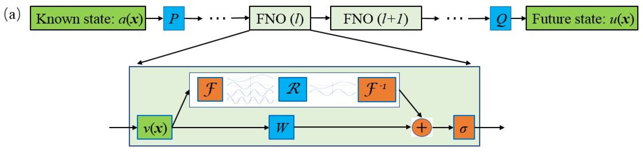
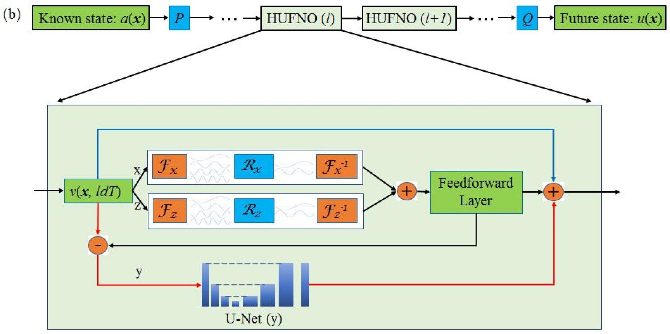
Figure 1: The configurations of (a) Fourier neural operator (FNO); and (b) hybrid U-Net and Fourier neural operator (HUFNO).

Letting $\mathcal{F}$ and $\mathcal{F}^{-1}$ denote the forward and reverse Fourier transforms of a function $f:D\rightarrow\mathbb{R}^{d_{v}}$ respectively, and substituting the kernel integral operator in Eq. 11 with a convolution operator defined in Fourier space, one can write the Fourier integral operator as

$$\left(\mathcal{K}(\phi)v_{m}\right)(\mathbf{x})=\mathcal{F}^{-1}\left(R_{\phi}\cdot\left(\mathcal{F}v_{m}\right)\right)(\mathbf{x}),\quad\forall\mathbf{x}\in D,$$ (12)

with $R_{\phi}$ being the Fourier transform of a periodic function $\mathcal{K}:\bar{D}\rightarrow\mathbb{R}^{d_{v}\times d_{v}}$ parameterized by $\phi\in\Theta_{\mathcal{K}}$. The frequency mode $k\in\mathbb{Z}^{d}$. The finite-dimensional parameterization can be obtained by truncating the Fourier series at mode $k_{\max}=\left|Z_{k_{\max}}\right|=\mid\left\{k\in\mathbb{Z}^{d}:\left|k_{j}\right|\leq k_{\max,j}\right.$, for $\left.j=1,\ldots,d\right\}\mid$. $\mathcal{F}\left(v_{m}\right)\in\mathbb{C}^{n\times d_{v}}$ is obtained by discretizing domain $D$ with $n\in\mathbb{N}$ points, where $v_{m}\in\mathbb{R}^{n\times d_{v}}$ [57]. By truncating the higher modes, $\mathcal{F}\left(v_{m}\right)\in\mathbb{C}^{k_{\max}\times d_{v}}$ can be obtained, where $\mathbb{C}$ is the complex space. $R_{\phi}$ is parameterized as complex-valued-tensor $({k_{\max}\times d_{v}\times d_{v}})$ containing a collection of truncated Fourier modes $R_{\phi}\in\mathbb{C}^{k_{\max}\times d_{v}\times d_{v}}$. Multiplying $R_{\phi}$ and $\mathcal{F}\left(v_{m}\right)$ yields

$$\left(R_{\phi}\cdot\left(\mathcal{F}v_{m}\right)\right)_{k,l}=\sum_{j=1}^{d_{v}}R_{\phi k,l,j}\left(\mathcal{F}v_{m}\right)_{k,j},\quad k=1,\ldots,k_{\max},\quad j=1,\ldots,d_{v}.$$ (13)

3.2 The hybrid U-Net and Fourier neural operator (HUFNO)

In this subsection, we first note that the original FNO framework adopts Fourier transform (and its inverse) in all three directions for 3D problems. As well known, this induces problems for non-periodic boundary conditions even though some ad hoc treatments would alleviate the problem [57, 97]. Recently, the work proposed by Tran et al. has shown that the FNO can be factorized into different directions and performed separately [82]. In this case, we can adopt the Fourier operations in the periodic directions while leaving the non-periodic direction(s) handled by the convolutional neural network (CNN). For the CNN, we choose the U-Net framework, which is originally designed for medical image segmentation tasks [104]. Due to its symmetrical encoder and decoder structure, U-Net can access low-level information and high-level features simultaneously in physical space [104, 105]. In this case, we hybridly combine the U-Net structure and FNO, leading to the hybrid U-Net and FNO (HUFNO) model. As we shall see, the HUFNO model outperforms both the original FNO and U-Net. The architecture of HUFNO is displayed in Fig. 1b. To construct the HUFNO model, we first define the operation $\mathcal{K}^{f}_{x,z}$as

$$\mathcal{K}^{f}_{x,z}(v_{l})=\mathcal{F}^{-1}_{x}[R_{x}\cdot\mathcal{F}_{x}(v_{l})]+\mathcal{F}^{-1}_{z}[R_{z}\cdot\mathcal{F}_{z}(v_{l})],$$ (14)

which contains the Fourier operations in the periodic $x$ and $z$ directions. Subsequently, the iterative updating procedure of $v(\mathbf{x})$ in HUFNO can be written as

$${v}_{l+1} =\mathcal{U}_{y}\{{v}_{l}-\mathcal{L}[\mathcal{K}^{f}_{x,z}({v}_{l})]\}+\mathcal{L}\{\mathcal{K}^{f}_{x,z}(v_{l})\}+{v}_{l},$$ (15)

where the U-Net operation, denoted by $\mathcal{U}_{y}$, is performed in the $y$ direction, and $\mathcal{L}$ is a two-layer feed forward operation defined as [82]

$$\mathcal{L}(v_{l})=\sigma\{W_{2}\sigma[W_{1}\mathcal{K}^{f}(v_{l})+b_{1}]+b_{2}\},$$ (16)

where $\sigma$ is a nonlinear activation function. As evident in Eq. 15, the non-periodicity is handled by the U-Net structure while the Fourier operations are only applied in the periodic directions. Meanwhile, a residual connection is additionally incorporated, allowing an easier flow of gradients.

4 Numerical tests in the turbulent flows over periodic hills

In this section, we test the performance of the newly proposed HUFNO framework in the LES of turbulent flows over periodic hills. The computational domain of the periodic hill flow is displayed in Fig. 2a, where the streamwise, vertical and spanwise dimensions of the domain $L_{x}=9h$, $L_{y}=3.036h$ and $L_{z}=4.5h$ [106]. The height of the hill is denoted by $h$. In this work, all length scales are normalized by the height of the hill, and the velocities are normalized by the bulk velocity above the crest of the hill. We note again that most of the existing test cases for FNO frameworks focus on simple geometries or flow conditions, including 2D Taylor Green vortex flows [57], 3D homogeneous isotropic turbulence (HIT) [83], turbulent mixing layer [87] and turbulent channel flows [97]. In contrast, the periodic hill turbulence possesses more complexity such as streamwise and normal non-homogeneity, normal non-periodicity, curved boundary, and strong flow separation. The generalization ability can also be tested by varying initial conditions and the shape of the hill.

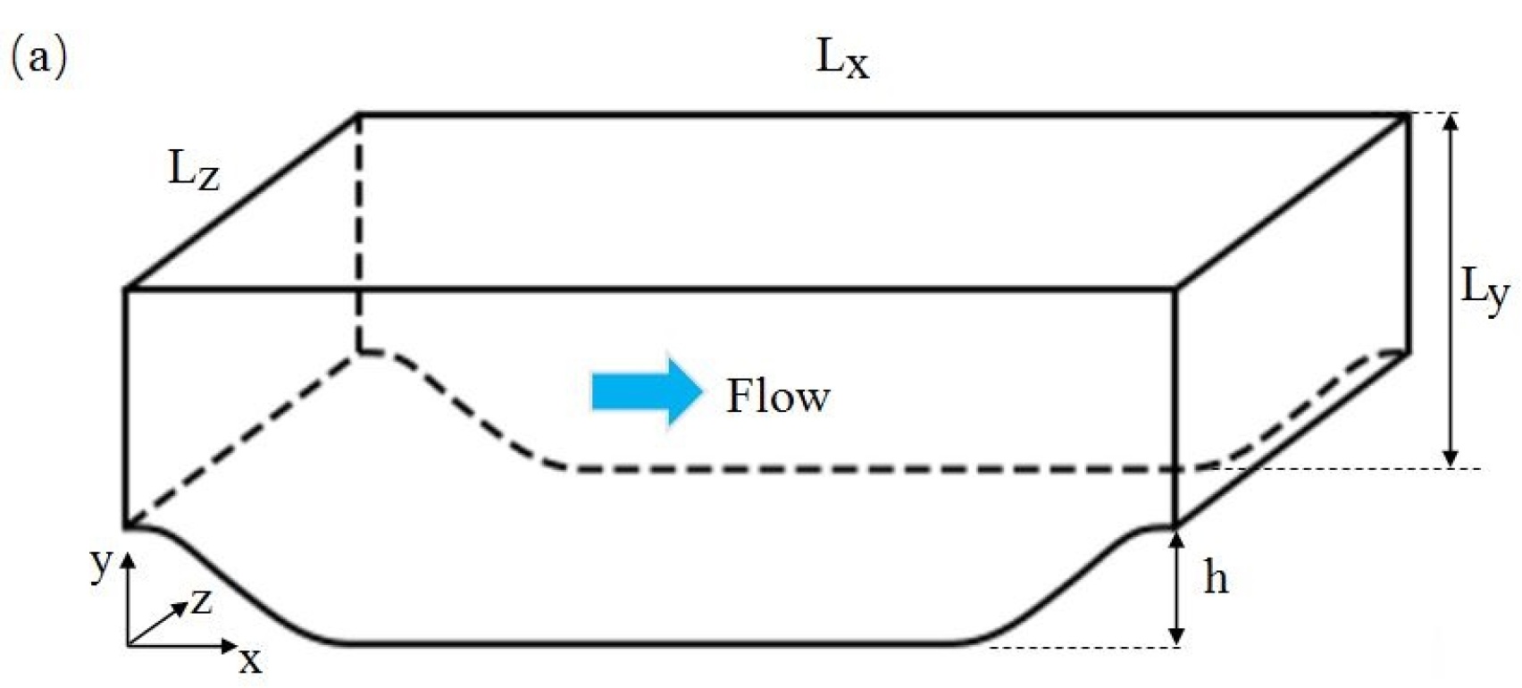
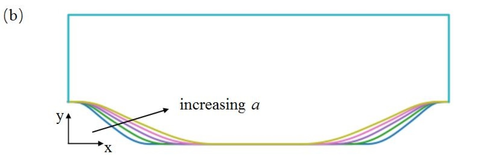
Figure 2: The computational domain of turbulent flow over periodic hill: (a) 3D view, (b) 2D view with varying shapes.

To obtain the training data as well as the benchmark data for LES, the DNS data for turbulent flows over periodic hills are coarsened to LES grids. In the a posteriori study, we compare the HUFNO-based solutions against the original FNO model, the U-Net, the benchmark DNS results as well as the traditional LES models. In the following sections, the DNS database and training data set are first introduced, followed by the a posteriori studies in the LES.

4.1 The DNS database for model training

The DNS database of turbulent flows over periodic hills are generated using the open-source framework Xcompact3D, which is a high-order compact finite-difference CFD solver [107, 108]. An immersed boundary method (IBM) method is adopted to account for the presence of the solid hills. Periodic boundary conditions are adopted in the streamwise and spanwise directions. No-slip conditions are applied at the upper wall and the surface of the hill. Since the values of the convolution kernels in the U-Net are local and constant, uniform grids are adopted in the simulations. This also lowers the error when coarsening the DNS flow field to LES grids. The shape of hill is defined by piecewise functions as follows:

First, we introduce a new streamwise coordinate variable $x_{L}$, and let

$$x_{L}=x,for\ x\leq 4.5,$$ (17)

and

$$x_{L}=9-x,for\ x>4.5.$$ (18)

Then we define the local height of the hill $y^{h}(x_{L})$ as

$$y^{h}(x_{L}) = min[1,1+5.312(x_{L}/a)^{2}-46.638(28x_{L}/a)^{3}],$$ (19)

$$\text{for}\ 0<x_{L}<0.321,$$

$$= 25.074+27.313(x_{L}/a)-79.664(x_{L}/a)^{2}+41.484(x_{L}/a)^{3},$$

$$\text{for}\ 0.321<x_{L}<0.5,$$

$$= 25.796+22.979(x_{L}/a)-70.994(x_{L}/a)^{2}+35.705(x_{L}/a)^{3},$$

$$\text{for}\ 0.5<x_{L}<0.714,$$

$$= 40.464-38.628(x_{L}/a)+15.256(x_{L}/a)^{2}-4.545(x_{L}/a)^{3},$$

$$\text{for}\ 0.714<x_{L}<1.071,$$

$$= 17.925+24.483(x_{L}/a)-43.648(x_{L}/a)^{2}+13.781(x_{L}/a)^{3},$$

$$\text{for}\ 1.071<x_{L}<1.429,$$

$$= max[0,56.390-56.295(x_{L}/a)+12.896(x_{L}/a)^{2}+0.587(x_{L}/a)^{3}],$$

$$\text{for}\ 1.429<x_{L}<1.929,$$

$$= 0,$$

$$\text{for}\ 1.929<x_{L}<4.5.{}$$

Here a shape parameter $a$ is introduced, such that the shape of hill can be varied as shown in Fig. 2b. A smaller value of $a$ indicates a steeper slope. With $a=1$, we recover the hill shape adopted by Breuer et al [106]. Detailed DNS parameters are given in Table 1. As well known, the prediction difficulty of turbulence increases with Reynolds number. In this study, three different Reynolds numbers are tested, namely $Re=700$, $1400$ and $5600$, such that the performance of the HUFNO model can be adequately assessed.

$Re$	Reso.	$\Delta x\times\Delta y\times\Delta z$	$h$	$\Delta t$
700	$128\times 129\times 64$	$0.070\times 0.024\times 0.070$	1.0	0.005
1400	$192\times 193\times 64$	$0.047\times 0.016\times 0.070$	1.0	0.005
5600	$768\times 385\times 128$	$0.012\times 0.004\times 0.035$	1.0	0.002

Table 1: Parameters for the direction numerical simulation of turbulent flows over periodic hill.

To verify the accuracy of the obtained DNS results, we compare the velocity statistics with the benchmark results by Breuer et al [106]. As displayed in Fig. 3, the mean velocities, the normal and shear Reynolds stresses are all consistent with the reference data of Breuer et al. at all three Reynolds numbers. Hence, the accuracy of the current DNS is confirmed. We also observe that although the turbulence statistics at different Reynolds numbers have some similarity, the influence of the Reynolds number is still evidenced especially in the near-wall regions.

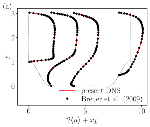
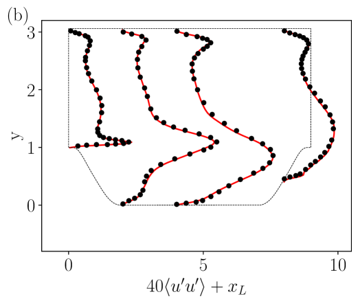
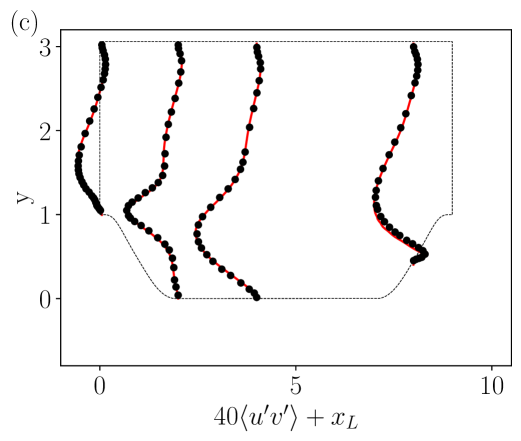
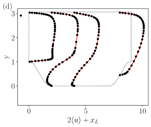
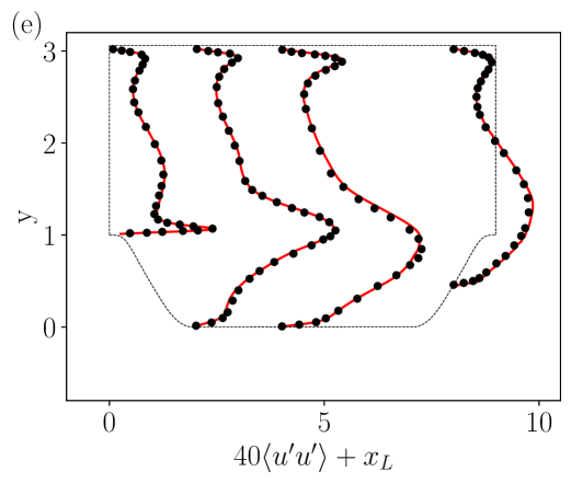
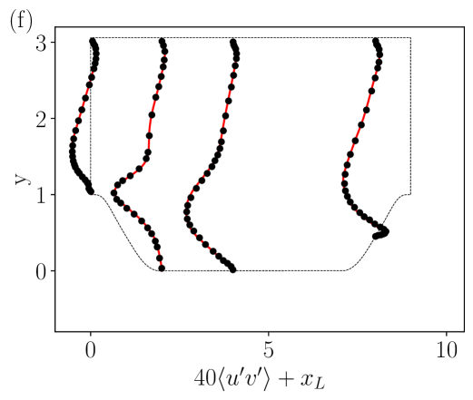
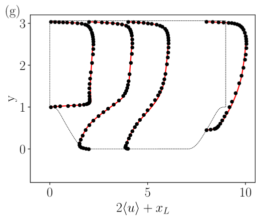
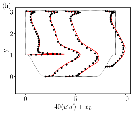
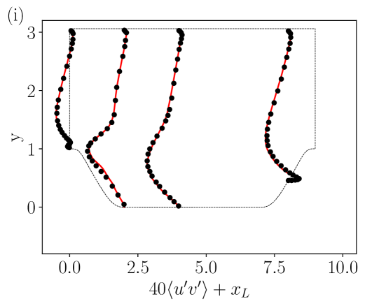
Figure 3: The mean streamwise velocity $\langle u\rangle$, the normal Reynolds stress $\langle u^{\prime}u^{\prime}\rangle$ and the shear Reynolds stress $\langle u^{\prime}v^{\prime}\rangle$ at different Reynolds numbers: the first, second and third rows represent the results at $Re=700$, $1400$ and $5600$, respectively; the first, second and third columns represent $\langle u\rangle$, $\langle u^{\prime}u^{\prime}\rangle$ and $\langle u^{\prime}v^{\prime}\rangle$, respectively.

4.2 Numerical experiments in the large-eddy simulation of periodic hill turbulence.

In the current work, the DNS data are coarsened to LES grids and taken as the benchmark for the LES. The grid information for LES is given in Table 2. In the training datasets, the DNS data are extracted at every $\Delta T=200\Delta t$ with $\Delta t$ being the DNS time step according to Table 1. Based on our tests, such configuration can give the best long-term performance. The known velocity fields and the shapes of the hill are taken as the input to the model. We take the known states (coarse-grained DNS data) of the previous five time nodes $[v(m-4),v(m-3),v(m-2),v(m-1),v(m)]$ as the model’s inputs and the increment $v(m+1)-v(m)$ as the model’s output. Five Fourier layers are adopted in the HUFNO framework. The Fourier modes are truncated at $k_{max}=5$, $5$ and $10$ for $Re=700$, $1400$ and $5600$, respectively, which are approximately 2/3 of the modes in the LES based the minimum grid numbers (i.e. in z direction). The width in the high-dimensional space after the projection of the inputs (cf. Fig. 1) is variably set to 80, and the batch size is 4. The Adam optimizer is adopted for optimization [109], the initial learning rate is set to $10^{-3}$ which decays by half after every 10 iterations, and the ReLU function is chosen as the nonlinear activation function [110]. The training and testing losses are defined by

$$\textit{Loss}=\frac{\|u^{*}-u\|_{2}}{\|u\|_{2}},\text{ where }\|\mathbf{A}\|_{2}=\frac{1}{n}\sqrt{\sum_{k=1}^{n}\left|\mathbf{A}_{\mathbf{k}}\right|^{2}},$$ (20)

where $u^{*}$ denotes the predicted variables and $u$ represents the corresponding value of ground truth.

In the a posteriori tests, the flow fields are initialized using unseen fully developed turbulent conditions. Meanwhile, zero-velocity conditions are reinforced to ensure physical consistency since the no-slip condition is not explicitly considered in the model. The prediction time step $\Delta T=200\Delta t$, which is consistent with the training process. A total of 400 time steps are simulated. The statistics are calculated by time averaging the results.

In the following sections, we test the performance of HUFNO in two scenarios: section 4.2.1 - varying the initial conditions with fixed hill shapes, and section 4.2.2 - varying the shape of the hill.

$Re$	Reso.	$\Delta x\times\Delta y\times\Delta z$
700	$32\times 33\times 16$	$0.281\times 0.095\times 0.281$
1400	$48\times 49\times 16$	$0.188\times 0.063\times 0.188$
5600	$64\times 65\times 32$	$0.141\times 0.047\times 0.141$

Table 2: Parameters for the large-eddy simulation of turbulent flows over periodic hill.

4.2.1 Test of varying the initial conditions with fixed hill shapes

In the tests for varied initial conditions, the hill shape is fixed at $a=1.0$. 20 groups of DNS datasets are generated using different initial conditions at each Reynolds number. In each simulation, 400 snapshots of the DNS data are extracted at every $\Delta T=200\Delta t$ for training the model. The evolution history of the training and testing losses for the FNO, U-Net and HUFNO models are shown in Fig. 4. As can be seen, the HUFNO model has the lowest testing losses compared to the FNO and U-Net models, while the losses of FNO are the highest. We also note that the differences between the training and testing losses are the largest for the U-Net model, indicating potential overfitting. Meanwhile, for all three models, the losses increase with Reynolds number, indicating the increased prediction difficulty with higher Reynolds number.

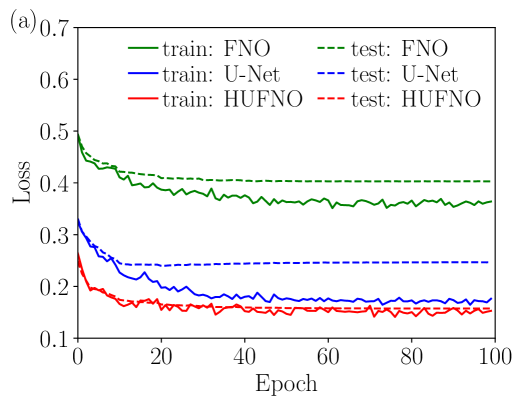
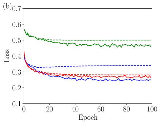
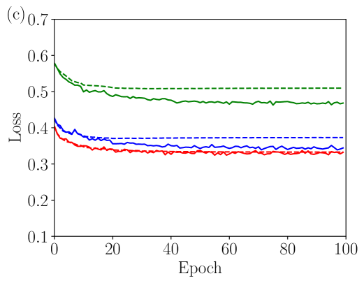
Figure 4: The evolutions of the loss curves: (a) $Re=700$; (b) $Re=1400$; (c) $Re=5600$.

In the a posteriori tests, initial conditions different from the training sets are used to initialize the flow field. In Fig. 5, we compare the predictions of the mean streamwise velocities, the normal and shear Reynolds stresses by different neural network (NN) models at different Reynolds numbers. Clearly, the HUFNO predictions have the closest agreements with the DNS benchmarks, underscoring its great efficacy. The FNO and U-Net have some small discrepancies at $Re=700$, while strongly deviate from the DNS results at high Reynolds numbers. The FNO model diverges at $Re=5600$, and hence the corresponding results are not shown in the figure. As the HUFNO model gives the best performance, only the results of HUFNO will be presented and compared against the traditional LES models in the rest of the paper.

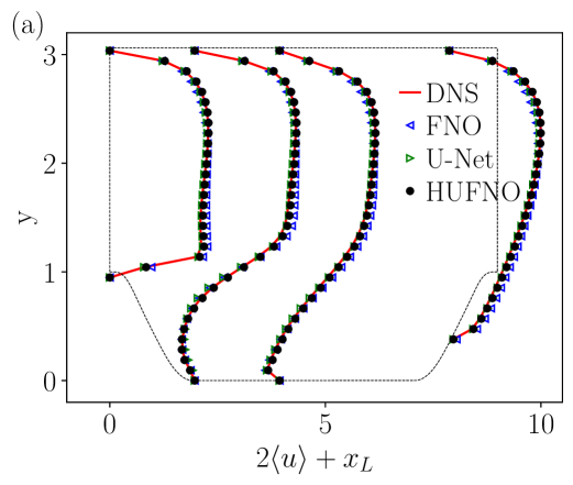
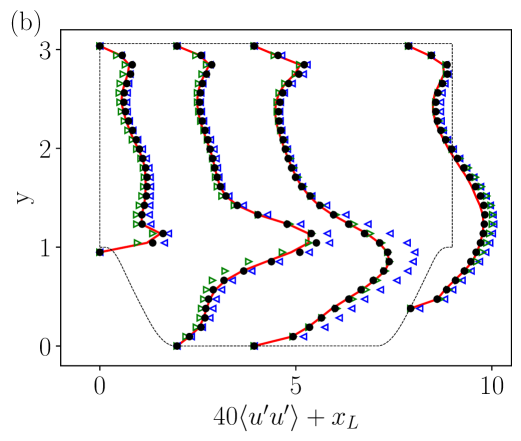
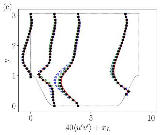
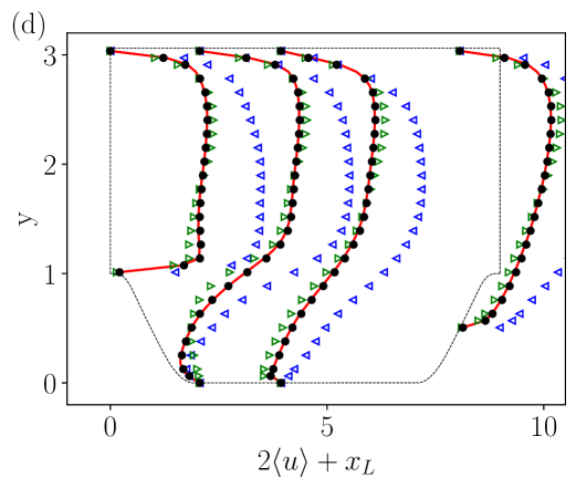
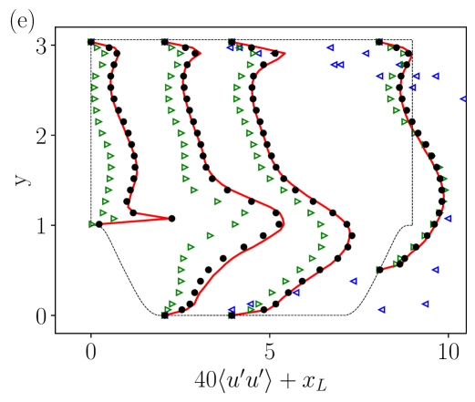
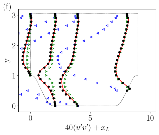
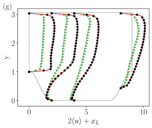
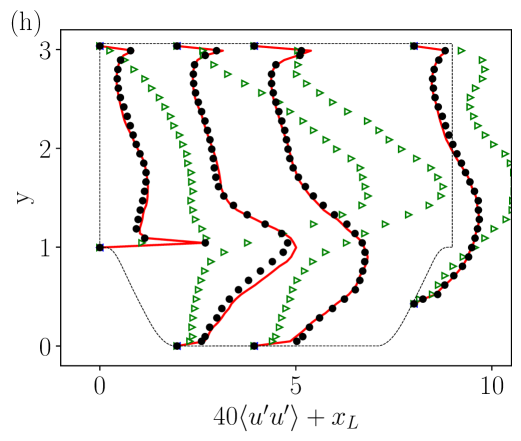
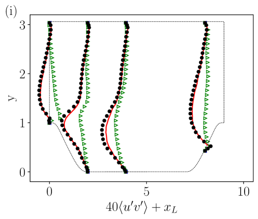
Figure 5: The predicted turbulence statistics by different neural network-based models in the LES at different Reynolds numbers: the first, second and third rows represent the results at $Re=700$, $1400$ and $5600$, respectively; the first, second and third columns represent $\langle u\rangle$, $\langle u^{\prime}u^{\prime}\rangle$ and $\langle u^{\prime}v^{\prime}\rangle$, respectively. The FNO model diverges at $Re=5600$, and thus the corresponding results are not shown in the third row.

The comparisons of the mean velocities and the Reynolds stresses between HUFNO model and the traditional LES results are shown in Fig. 6. Here the SMAG and WALE models are adopted in the traditional LES. As the figure depicts, the HUFNO model performs reasonably better at all three Reynolds numbers compared to the SMAG and WALE models. Meanwhile, we observe that the WALE model can also predict the mean velocity very well, demonstrating its advantage over the SMAG model. However, in the predictions of the Reynolds stresses, both the SMAG and WALE models have noticeable deviations from the DNS results.

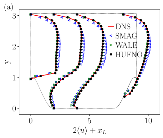
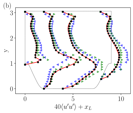
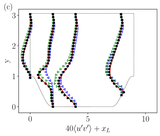
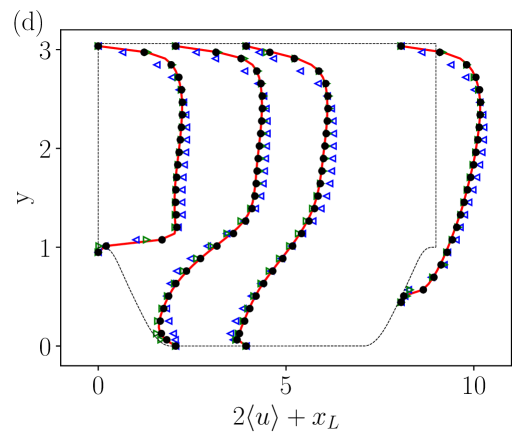
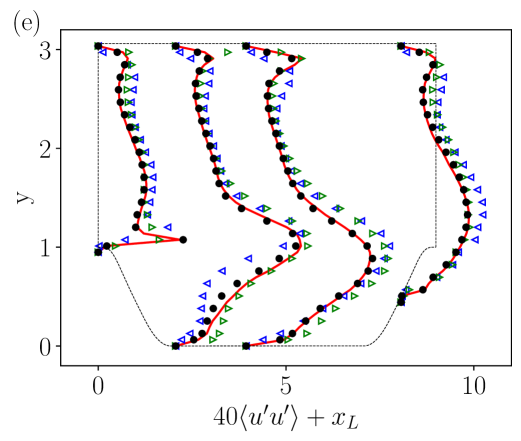
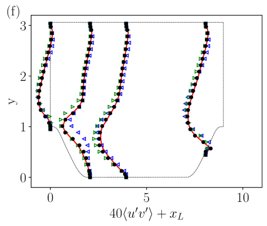
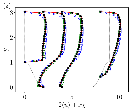
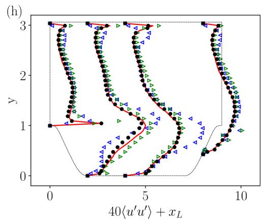
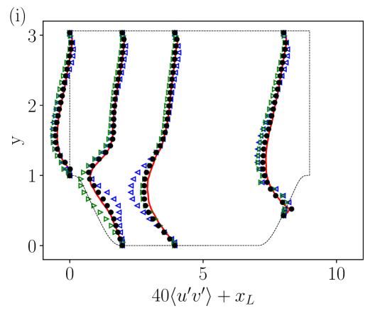
Figure 6: The predicted turbulence statistics by the HUFNO model and the traditional LES: the first, second and third rows represent the results at $Re=700$, $1400$ and $5600$, respectively; the first, second and third columns represent the results for $\langle u\rangle$, $\langle u^{\prime}u^{\prime}\rangle$ and $\langle u^{\prime}v^{\prime}\rangle$, respectively.

To examine the energy distribution at different length scales, we calculate the streamwise kinetic energy spectrum in the LES. The results are shown in Figs. 7a, 7b and 7c for $Re=700$, $1400$ and $5600$, respectively. At $Re=700$, the predicted spectrum by the HUFNO model agrees well with the DNS result. Both the SMAG and WALE models overestimate the large-scale energy while underestimate the small-scale energy. At $Re=1400$ and $5600$, the agreements between HUFNO and DNS are slightly worse compared to the case of $Re=700$, indicating increased prediction difficulty at higher Reynolds numbers. Nevertheless, the HUFNO model still tangibly outperforms the traditional SMAG and WALE models.

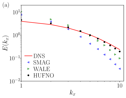
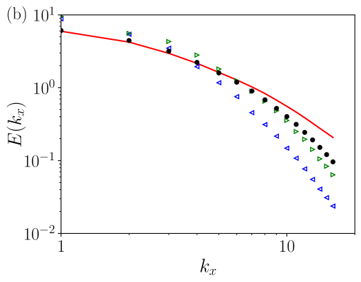
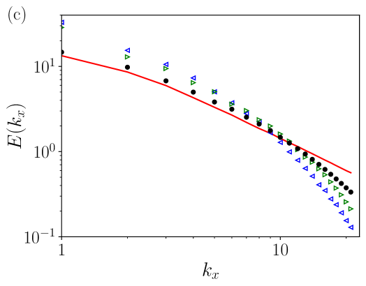
Figure 7: The streamwise energy spectra at various Reynolds numbers: (a) $Re=700$; (b) $Re=1400$; (c) $Re=5600$.

To assess the quality of predictions near the wall, we examine the dimensionless viscous wall-shear stress in the flow separation region. The wall-shear stress is calculated as $\langle\tau^{W}_{xy}\rangle=\langle\partial u/\partial y\rangle/Re$ at $y=h$. The results are displayed in Fig. 8. The intersection of the wall-shear stress and zero indicates the extents of the flow separation region. Compared to the traditional LES models, the HUFNO can more accurately predict of the distribution of wall-shear stress on the hill surface. Meanwhile, the WALE model tangibly outperforms the SMAG model due to its physically consistent treatment of near-wall eddy viscosity [101].

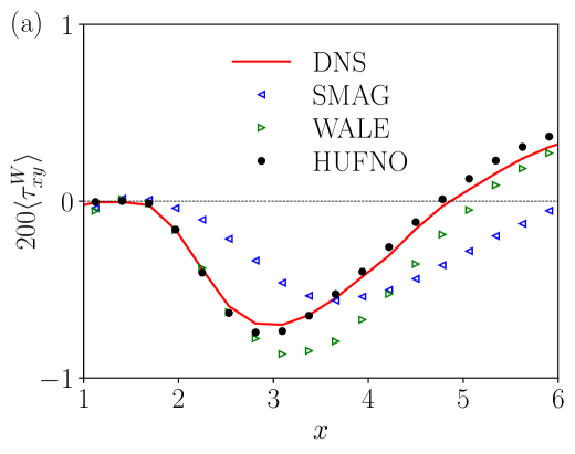
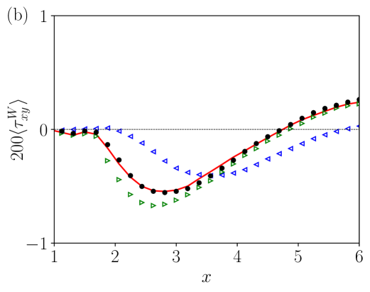
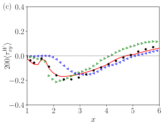
Figure 8: The predicted wall-shear stress $\langle\tau^{W}_{xy}\rangle$ in the flow separation region: (a) $Re=700$; (b) $Re=1400$; (c) $Re=5600$.

To visualize the predicted spatial structures of the turbulent flow over periodic hills, we present the streamlines of the flow field in Figs. 9, 10 and 11 for $Re=700$, $1400$ and $5600$, respectively. The contours are colored by the streamwise velocities. The separation regions and the re-circulation streamlines can be clearly identified. As observed, the HUFNO model gives the best predictions for the flow separations at all three Reynolds numbers, demonstrating its accuracy for predicting strongly separated flows.

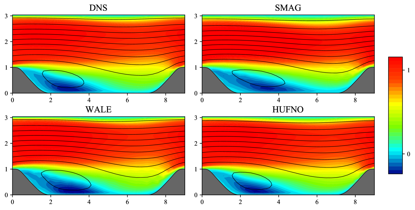
Figure 9: The streamlines of the periodic hill flow at $Re=700$. The domain is colored by the streamwise velocity.

Figure 10: The streamlines of the periodic hill flow at $Re=1400$. The domain is colored by the streamwise velocity.

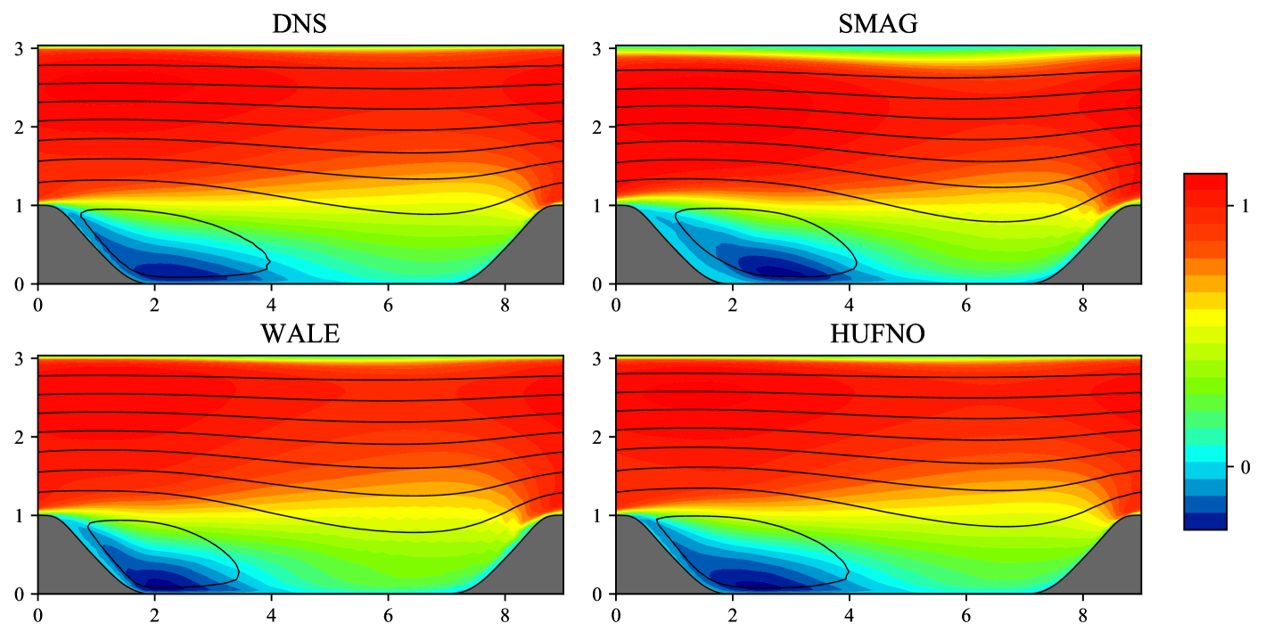
Figure 11: The streamlines of the periodic hill flow at $Re=5600$. The domain is colored by the streamwise velocity.

In Table 3, we list the computational costs for the HUFNO model and traditional LES models. Shown in the table are the computation times in seconds for equivalent 10000 DNS time steps. The HUFNO-based simulations are conducted on the NVIDIA A100 GPU, for which the CPU configuration is AMD EPYC 7763 @2.45GHz. The traditional LES simulations using the SMAG and WALE models are performed on the CPU of Intel Xeon Gold 6148 @2.40 GHz. As evidenced in the table, the computational efficiency of the HUFNO model is considerably higher than those of the traditional LES models. Here we note that the computational costs of the traditional LES models in the table are not multiplied by the number of adopted computational cores (given in the parentheses).

$Re$	SMAG	WALE	HUFNO
700	66.23s ($\times$64 cores)	74.77s ($\times$64 cores)	2.02s
1400	232.14s ($\times$64 cores)	249.71s ($\times$64 cores)	2.23s
5600	270.00s ($\times$64 cores)	391.43 ($\times$64 cores)	6.33s

Table 3: Computational costs of different LES models per 10000 DNS time step.

4.2.2 Test of varying the shape of the hill

In this section, we further test the generalization ability of the proposed HUFNO model for hill shapes different from the training ones. For this purpose, we design the training and testing cases as follows. The shape factors $a$ (cf. Eq. 4.1) in the training set are chosen at $a=1.0,1.2,1.4,1.6,1.8$, each of which contains 10 different initial conditions. In this case, the training set contains 50 simulation results in total. The other training configurations remain the same as in the test for varying initial conditions. This test is conducted at $Re=700$ for demonstration. The training and testing losses are displayed in Fig. 12, and the testing loss saturates well with 100 epochs.

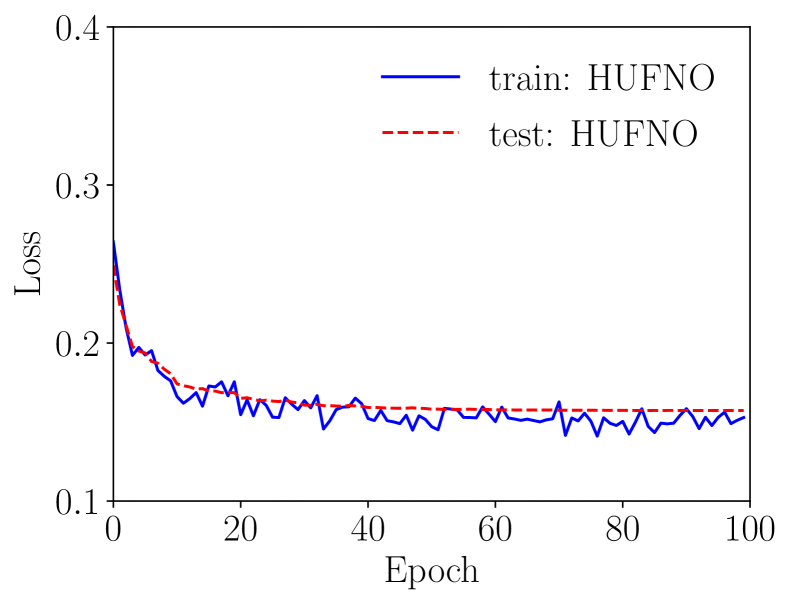
Figure 12: The evolutions of the loss curves in the training for varying hill slopes.

In the a posteriori LES tests, we choose the shape factors $a=0.9,1.5$ and $1.9$, of which $0.9$ represents a hill slope steeper than all those training ones, $1.5$ represents a interpolated shape, and $1.9$ represents a milder slope. The predicted mean velocities and Reynolds stresses for the new hill shapes are displayed in Fig. 13. The corresponding predictions by the traditional SMAG and WALE models are also shown in the figure. As can be seen, at all three new hill shapes, the HUFNO model performs better than the SMAG and WALE models, both of which show some discrepancies from the DNS benchmark, especially in the predictions of the Reynolds stresses.

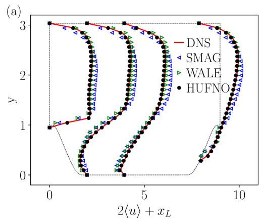
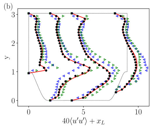
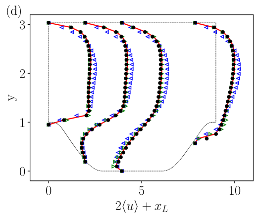
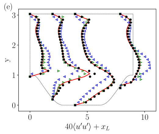
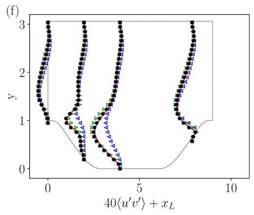
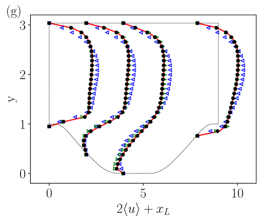
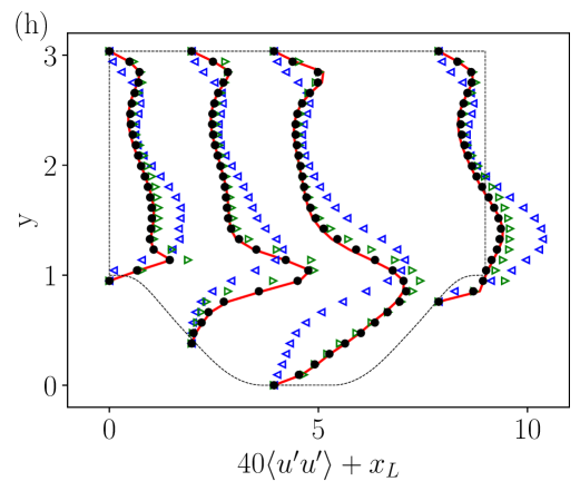
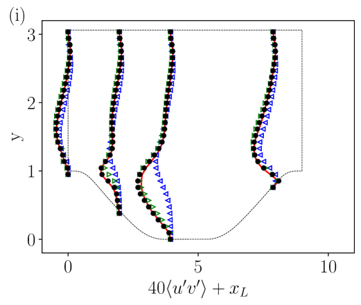
Figure 13: The predicted turbulence statistics by the HUFNO model and the traditional LES with varying hill shapes: the first, second and third rows represent the results for shape factors $a=0.9$, $1.5$ and $1.9$, respectively; the first, second and third columns represent the results for $\langle u\rangle$, $\langle u^{\prime}u^{\prime}\rangle$ and $\langle u^{\prime}v^{\prime}\rangle$, respectively.

The predicted streamwise energy spectra by different models in the LES are shown in Figs. 14a, 14b and 14c for $a=0.9$, $1.5$ and $1.9$, respectively. As shown in the figures, the predicted spectra by the HUFNO model agree well with the DNS results at all three unseen shapes of the hill, while pronounced deviations from the DNS results can be observed in the predictions by the SMAG and WALE models.

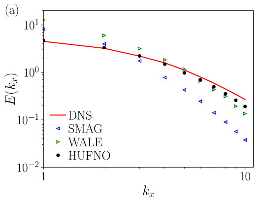
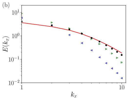
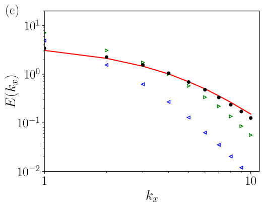
Figure 14: The streamwise energy spectra at $Re=700$ for various hill shapes: (a) $a=0.9$; (b) $a=1.5$; (c) $a=1.9$.

Undoubtedly, the change of the hill shape would affect the wall shear stress as displayed in Fig. 15. Overall, the HUFNO model gives the best prediction of the wall shear stress at all three hill shapes, even though the prediction accuracy is slightly decreased compared to the scenario when only the initial condition is varied (cf. Fig. 8). This is not surprising since generalizing to different boundary shapes is inherently more challenging than generalizing to different initial conditions. Meanwhile, we observe that the separation zone extends farther downstream as the slopes become milder, indicating the strong influence of the hill shape on flow separation. Again, the WALE model tangibly outperforms the SMAG model due to its near-wall considerations in the formulation [101].

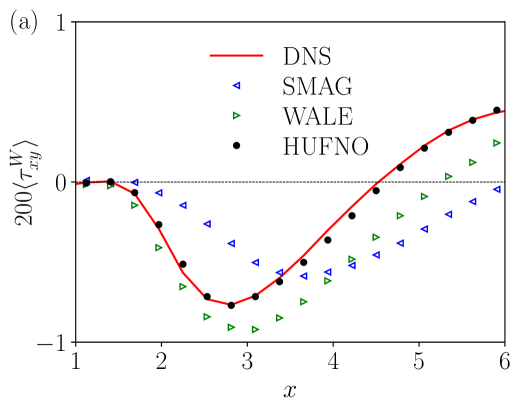
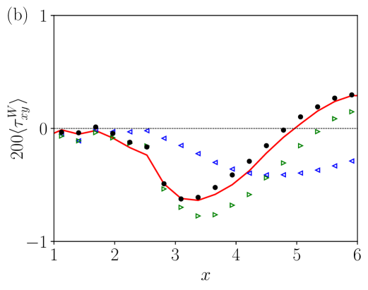
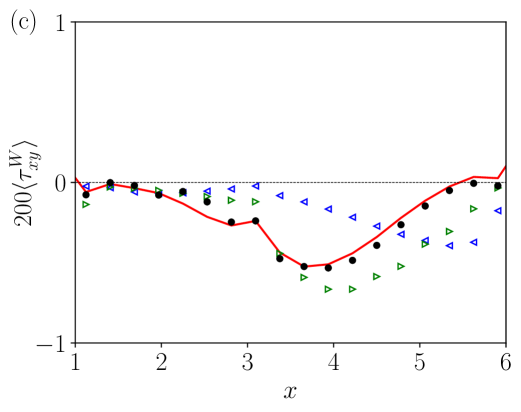
Figure 15: The predicted wall-shear stress $\langle\tau^{W}_{xy}\rangle$ in the flow separation region for varying hill shapes: (a) $a=0.9$; (b) $a=1.5$; (c) $a=1.9$.

Finally, we examine the predicted streamlines and the velocity structures of the periodic hill flow field in Figs. 16, 17 and 18 for $a=0.9$, $1.5$ and $1.9$, respectively. The contours are colored by the streamwise velocities. We observe that the shape of the hills significantly affect the size and shape of the separation bubbles and the re-circulation streamlines. A milder slope gives a longer and slimmer separation region. As expected, the HUFNO model gives the best predictions for the flow separations at all three new hill shapes, underscoring its generalization ability in predicting the separated turbulent flows over periodic hills of unseen shapes.

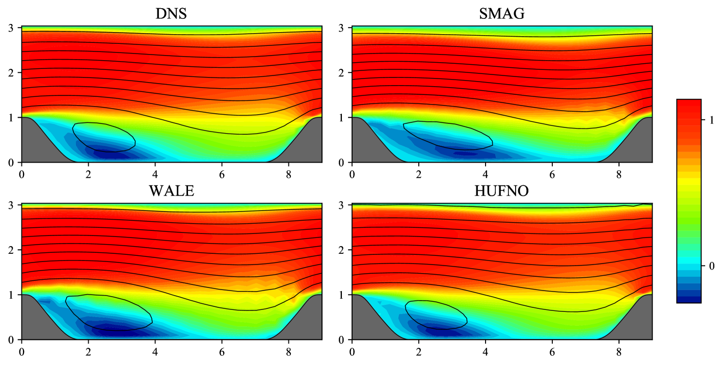
Figure 16: The streamlines of the periodic hill flow at $Re=700$ with shape factor $a=0.9$. The domain is colored by the streamwise velocity.

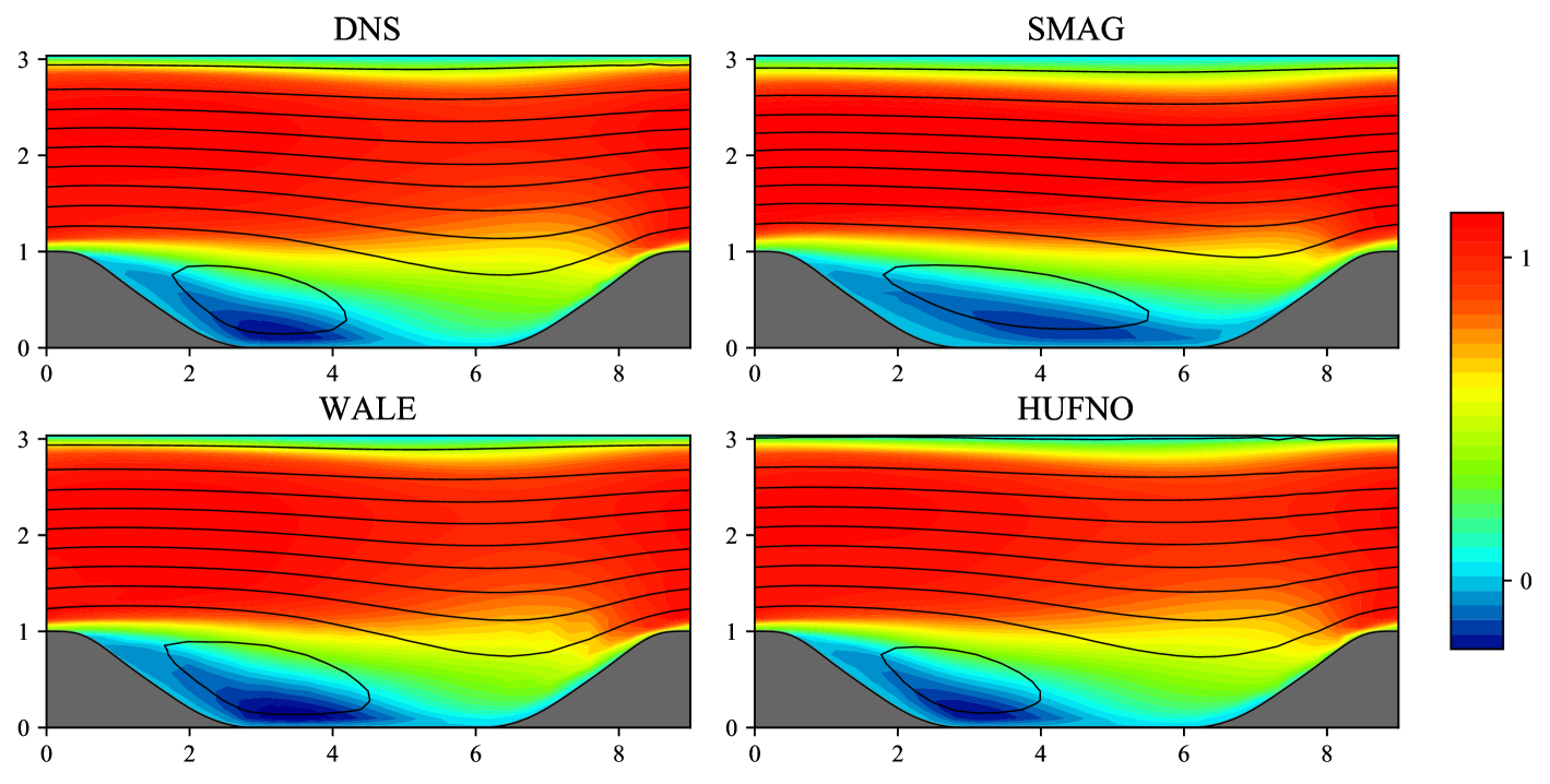
Figure 17: The streamlines of the periodic hill flow at $Re=700$ with shape factor $a=1.5$. The domain is colored by the streamwise velocity.

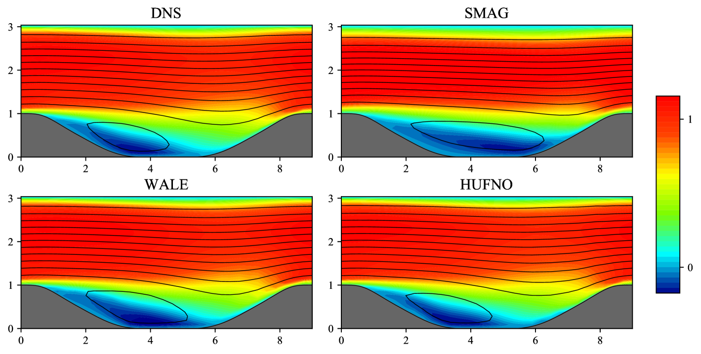
Figure 18: The streamlines of the periodic hill flow at $Re=700$ with shape $a=1.9$. The domain is colored by the streamwise velocity.

5 Conclusions

In this study, the hybrid framework of U-Net and Fourier neural operator (HUFNO) is proposed and tested in the large-eddy simulations (LES) of turbulent flows over periodic hills. By integrating the advantages of the U-Net and Fourier neural operator (FNO), the proposed model is specially tailored for problems with mixed periodic and non-periodic boundary conditions. Our preliminary test shows that the HUFNO model outperforms the original FNO model as well as the U-Net model in the predictions of the turbulent velocity statistics and Reynold stresses. In the a posteriori tests of LES, the flow prediction capacity of the HUFNO framework is evaluated against the DNS benchmark and the traditional LES simulations using the classical SMAG and WALE models.

In the LES, the performance of the HUFNO framework is tested in two scenarios: at initial conditions different from the training set with fixed hill shape; and at new hill shapes. Compared to the traditional SMAG and WALE models-based LES, the newly proposed HUFNO model can predict better the mean velocity, the Reynolds stress, the energy spectrum and the wall-shear stresses. Meanwhile, the WALE model tangibly outperforms the SMAG model due to its inherent near-wall considerations in the formulation.

The streamlines and velocity contour of the flow field are examined to assess the ability of the HUFNO model in predicting the spatial structures of the periodic hill turbulence. Both the separation bubbles and re-circulation streamlines can be more accurately predicted by the HUFNO model compared to the traditional LES models. Further, the computational costs of the HUFNO models are considerably lower than the traditional LES, demonstrating its great efficiency.

Finally, it is worth noting that while the current work demonstrates the potential of HUFNO in the prediction of turbulent flows over periodic hills, challenges still exist in many aspects for machine learning-based flow solvers, such as complex turbulent flows at high Reynolds numbers, irregular and non-Cartesian grids, and the situations when training data is limited. To address these difficulties, many aspects can be considered in future works, such as incorporating physical constraints to lower the data requirement [74, 111, 112], using geometry-informed neural operators (GINO) to handle complex geometries [85], and data assimilation [113, 19], etc.

6 Acknowledgments

This work was supported by the National Natural Science Foundation of China (NSFC Grants No. 12302283, No. 12172161, No. 92052301, No. 12161141017, and No. 91952104), by the NSFC Basic Science Center Program (Grant No. 11988102), by the Shenzhen Science and Technology Program (Grant No. KQTD20180411143441009), by Key Special Project for Introduced Talents Team of Southern Marine Science and Engineering Guangdong Laboratory (Guangzhou) (Grant No. GML2019ZD0103), by Department of Science and Technology of Guangdong Province (Grants No. 2019B21203001, No. 2020B1212030001, and No.2023B1212060001), by the Shandong Province Youth Fund Project (Grant No. ZR20240A050), and by the Natural Science Foundation of Hainan Province (Grant No. 425QN376). This work was also supported by Center for Computational Science and Engineering of Southern University of Science and Technology, and by National Center for Applied Mathematics Shenzhen (NCAMS).

References

- Pope et al. [2000] S. B. Pope, Turbulent Flows (Cambridge University Press, 2000).
- Bauweraerts et al. [2021] P. Bauweraerts, and J. Meyers, Reconstruction of turbulent flow fields from lidar measurements using large-eddy simulation, J. Fluid Mech. 906, A17 (2021).
- Meneveau et al. [2000] C. Meneveau, and J. Katz, Scale-invariance and turbulence models for large-eddy simulation, Annu. Rev. Fluid Mech. 32, 1 (2000).
- Moser et al. [2021] R. D. Moser, S. W. Haering, and G. R. Yalla, Statistical properties of subgrid-scale turbulence models, Annu. Rev. Fluid Mech. 53, 255-286 (2021).
- Yang et al. [2021] X. I. A. Yang, and K. P. Griffin, Grid-point and time-step requirements for direct numerical simulation and large-eddy simulation, Phys. Fluids 33, 015108 (2021).
- Duraisamy et al. [2019] K. Duraisamy, G. Iaccarino, and H. Xiao, Turbulence modeling in the age of data, Annu. Rev. Fluid Mech. 51, 537 (2019).
- Jiang et al. [2021] C. Jiang, R. Vinuesa, R. Chen, J. Mi, S. Laima, and H. Li, An interpretable framework of data-driven turbulence modeling using deep neural networks, Phys. Fluids 33, 055133 (2021).
- Durbin et al. [2018] P. A. Durbin, Some recent developments in turbulence closure modeling, Annu. Rev. Fluid Mech. 50, 77 (2018).
- Pope et al. [1975] S. B. Pope, A more general effective-viscosity hypothesis, J. Fluid Mech. 72, 331-340 (1975).
- Chen et al. [2023] P. E. S. Chen, W. Wu, K. P. Griffin, Y. Shi, and X. I. A. Yang, A universal velocity transformation for boundary layers with pressure gradients, J. Fluid Mech. 970, A3 (2023).
- Bin et al. [2024] Y. Bin, X. Hu, J. Li, S. J. Grauer, and X. I. A. Yang, Constrained re-calibration of two-equation Reynolds-averaged Navier–Stokes models, Theor. App. Mech. Lett. doi: https://doi.org/10.1016/j.taml.2024.100503 (2024).
- Pinier et al. [2021] B. Pinier, R. Lewandowski, E. Mémin, and P. Chandramouli, Testing a one-closure equation turbulence model in neutral boundary layers, Comput. Methods Appl. Mech. Eng. 376, 113662 (2021).
- Smagorinsky et al. [1963] J. Smagorinsky, General circulation experiments with the primitive equations, i. the basic experiment, Mon. Weath. Rev. 91, 99 (1963).
- Lilly et al. [1967] D. K. Lilly, The representation of small-scale turbulence in numerical simulation experiments, In Proc. IBM Scientific Computing Symp. on Environmental Sciences pp, 195 (1967).
- Deardorff et al. [1970] J. W. Deardorff, A numerical study of three-dimensional turbulent channel flow at large Reynolds numbers, J. Fluid Mech. 41, 453 (1970).
- Sagaut et al. [2006] P. Sagaut, Large eddy simulation for incompressible flows (Berlin Heidelberg: Springer, 2006).
- Moin et al. [1991] P. Moin, K. Squires, W. Cabot, and S. Lee, A dynamic subgrid-scale model for compressible turbulence and scalar transport, Phys. Fluids A 3, 2746 (1991).
- Germano et al. [1992] M. Germano, Turbulence: The filtering approach, J. Fluid Mech. 238, 325 (1992).
- Mons et al. [2021] V. Mons, Y. Du, and T. A. Zaki, Ensemble-variational assimilation of statistical data in large-eddy simulation, Phys. Rev. Fluids 6, 104607 (2021).
- Rouhi et al. [2016] A. Rouhi, U. Piomelli, and B. J. Geurts, Dynamic subfilter-scale stress model for large-eddy simulations, Phys. Rev. Fluids 1, 044401 (2016).
- Celora et al. [2021] T. Celora, N. Andersson, I. Hawke, and G. L. Comer, Covariant approach to relativistic large-eddy simulations: The fibration picture, Phys. Rev. D 104, 084090 (2021).
- Rozema et al. [2022] W. Rozema, H. J. Bae, and R. W. C. P. Verstappen, Local dynamic gradient Smagorinsky model for large-eddy simulation, Phys. Rev. Fluids 7, 074604 (2022).
- Park et al. [2021] J. Park, and H. Choi, Toward neural-network-based large eddy simulation: application to turbulent channel flow, J. Fluid Mech. 914, A16 (2021).
- Guan et al. [2022] Y. Guan, A. Chattopadhyay, A. Subel, and P. Hassanzadeh, Stable a posteriori LES of 2D turbulence using convolutional neural networks: Backscattering analysis and generalization to higher Re via transfer learning, J. Comput. Phys. 458, 111090 (2022).
- Novati et al. [2021] G. Novati, H. L. de Laroussilhe, and P. Koumoutsakos, Automating turbulence modelling by multi-agent reinforcement learning, Nat. Mach. Intell. 3, 87–96 (2021).
- Bae et al. [2022] H. J. Bae, and P. Koumoutsakos, Scientific multi-agent reinforcement learning for wall-models of turbulent flows, Nat. Commun. 13, 1443 (2022).
- Wu et al. [2024] H. Wu, F. Xu, Y. Duan, Z. Niu, W. Wang, G. Lu, K. Wang, Y. Liang, and Y. Wang, Spatio-Temporal Fluid Dynamics Modeling via Physical-Awareness and Parameter Diffusion Guidance, arXiv:2403.13850 (2024).
- Li et al. [2024] T. Li, L. Biferale, F. Bonaccorso, M. A. Scarpolini, and M. Buzzicotti, Synthetic Lagrangian turbulence by generative diffusion models, Nat. Mach. Intell. 6, 393–403 (2024).
- Wang et al. [2022] X. Wang, J. Q Kou, and W. W. Zhang, Unsteady aerodynamic prediction for iced airfoil based on multi-task learning, Phys. Fluids 34, 087117 (2022).
- Mohamed et al. [2023] A. Mohamed, and D. Wood, Deep learning predictions of unsteady aerodynamic loads on an airfoil model pitched over the entire operating range, Phys. Fluids 35, 053113 (2023).
- Kurtulus et al. [2009] D. F. Kurtulus, Ability to forecast unsteady aerodynamic forces of flapping airfoils by artificial neural network, Neural Comput. Appl. 18, 359-368 (2009).
- Wu et al. [2018] J. L. Wu, H. Xiao, and E. Paterson, Physics-informed machine learning approach for augmenting turbulence models: A comprehensive framework, Phys. Rev. Fluids 3, 074602 (2018).
- Ling et al. [2016] J. Ling, A. Kurzawski, and J. Templeton, Reynolds averaged turbulence modelling using deep neural networks with embedded invariance, J. Fluid Mech. 807, 155 (2016).
- Wang et al. [2017] J. X. Wang, J. L. Wu, and H. Xiao, Physics-informed machine learning approach for reconstructing Reynolds stress modeling discrepancies based on dns data, Phys. Rev. Fluids 2, 034603 (2017).
- Wu et al. [2019] J. L. Wu, H. Xiao, R. Sun, and Q. Q. Wang, Reynolds averaged Navier Stokes equations with explicit data driven Reynolds stress closure can be ill conditioned, J. Fluid Mech. 869, 553-586 (2019).
- Yang et al. [2019] X. I. A. Yang, S. Zafar, J. X. Wang, and H. Xiao, Predictive large-eddy-simulation wall modeling via physics-informed neural networks, Phys. Rev. Fluids 4, 034602 (2019).
- Gamahara et al. [2017] M. Gamahara, and Y. Hattori, Searching for turbulence models by artificial neural network, Phys. Rev. Fluids 2(5), 054604 (2017).
- Yuan et al. [2021] Z. Yuan, Y. Wang, C. Xie, and J. Wang, Deconvolutional artificial-neuralnetwork framework for subfilter-scale models of compressible turbulence, Acta Mech. Sin. 37, 1773–1785 (2021).
- Xie et al. [2019] C. Xie, K. Li, C. Ma, and J. Wang, Modeling subgrid-scale force and divergence of heat flux of compressible isotropic turbulence by artificial neural network, Phys. Rev. Fluids 4, 104605 (2019).
- Xie et al. [2019] C. Xie, J. Wang, K. Li, and C. Ma, Artificial neural network approach to large-eddy simulation of compressible isotropic turbulence, Phys. Rev. E 99, 053113 (2019).
- Xie et al. [2020] C. Xie, J. Wang, and W. E, Modeling subgrid-scale forces by spatial artificial neural networks in large eddy simulation of turbulence, Phys. Rev. Fluids. 5, 054606 (2020).
- Beck et al. [2019] A. Beck, D. Flad, and C. D. Munz, Deep neural networks for data-driven turbulence models, J. Comput. Phys. 398, 108910 (2019).
- Maulik et al. [2017] R. Maulik, and O. San, A neural network approach for the blind deconvolution of turbulent flow, J. Fluid Mech. 831, 151–181 (2017).
- Maulik et al. [2019] R. Maulik, O. San, A. Rasheed, and P. Vedula, Subgrid modelling for two-dimensional turbulence using neural networks, J. Fluid Mech. 858, 122 (2019).
- Kurz et al. [2023] M. Kurz, P. Offenhaeuser, and A. Beck, Deep reinforcement learning for turbulence modeling in large eddy simulations, Int. J. Heat Fluid Flow 99, 109094 (2023).
- Zhou et al. [2019] Z. Zhou, G. He, S. Wang, and G. Jin, Subgrid-scale model for large-eddy simulation of isotropic turbulent flows using an artificial neural network, Computers Fluids 195, 104319 (2019).
- Xu et al. [2023] D. Xu, J. Wang, C. Yu, and S. Chen, Artificial-neural-network-based nonlinear algebraic models for large-eddy simulation of compressible wall-bounded turbulence, J. Fluid Mech. 960, A4 (2023).
- Prakash et al. [2024] A. Prakash, K. E. Jansen, and J. A. Evans, Invariant data-driven subgrid stress modeling on anisotropic grids for large eddy simulation, Comput. Methods Appl. Mech. Eng. 422, 116807 (2024).
- LozanoDuran et al. [2023] A. Lozano-Durán, and H. J. Bae, Machine learning building-block-flow wall model for large-eddy simulation, J. Fluid Mech. 963, A35 (2023).
- Vadrot et al. [2023] A. Vadrot, X. I. A. Yang, and M. Abkar, Survey of machine-learning wall models for large-eddy simulation, Phys. Rev. Fluids. 8, 064603 (2023).
- Li et al. [2023] T. Li, M. Buzzicotti, F. Bonaccorso, L. Biferale, S. Chen, and M. Wan, Multi-scale reconstruction of turbulent rotating flows with proper orthogonal decomposition and generative adversarial networks, J. Fluid Mech. 971, A3 (2023).
- Buzzicotti et al. [2021] M. Buzzicotti, F. Bonaccorso, P. Clark Di Leoni, and L. Biferale, Reconstruction of turbulent data with deep generative models for semantic inpainting from TURB-Rot database, Phys. Rev. Fluids. 6, 050503 (2021).
- Guastoni et al. [2021] L. Guastoni, A. Güemes, A. Ianiro, S. Discetti, P. Schlatter, H. Azizpour, and R. Vinuesa, Convolutional-network models to predict wall-bounded turbulence from wall quantities, J. Fluid Mech. 928, A27 (2021).
- Zhu et al. [2024] L. Zhu, X. Jiang, A. Lefauve, R. R. Kerswell, and P. F. Linden, New insights into experimental stratified flows obtained through physics-informed neural networks, J. Fluid Mech. 981, R1 (2024).
- Deng et al. [2019] Z. Peng, C. He, Y. Liu, and K. C. Kim, Super-resolution reconstruction of turbulent velocity fields using a generative adversarial network-based artificial intelligence framework, Phys. Fluids 31, 125111 (2023).
- Kim et al. [2021] H. Kim, K. Kim, J. Won, and C. Lee, Unsupervised deep learning for super-resolution reconstruction of turbulence, J. Fluid Mech. 910, A29 (2021).
- Li et al. [2020] Z. Li, N. Kovachki, K. Azizzadenesheli, B. Liu, K. Bhattacharya, A. Stuart, and A. Anandkumar, Fourier neural operator for parametric partial differential equations, arXiv:2010.08895 (2020).
- Li et al. [2020] Z. Li, D. Z. Huang, B. Liu, and A. Anandkumar, Fourier Neural Operator with Learned Deformations for PDEs on General Geometries, arXiv:2207.05209 (2022).
- Deng et al. [2023] Z. Deng, H. Liu, B. Shi, Z. Wang, F. Yu, Z. Liu, and G. Chen, Temporal predictions of periodic flows using a mesh transformation and deep learning-based strategy, Aerosp. Sci. Technol 134, 108081 (2023).
- Peng et al. [2022] W. Peng, Z. Yuan, and J. Wang, Attention-enhanced neural network models for turbulence simulation, Phys. Fluids 34, 025111 (2022).
- Peng et al. [2023] W. Peng, Z. Yuan, Z. Li, and J. Wang, Linear attention coupled Fourier neural operator for simulation of three-dimensional turbulence, Phys. Fluids 35, 015106 (2023).
- Lienen et al. [2023] M. Lienen, D. Lüdke, J. Hansen-Palmus, and S. Günnemann, From Zero to Turbulence: Generative Modeling for 3D Flow Simulation, arXiv:2306.01776 (2023).
- Bukka et al. [2021] S. R. Bukka, R. Gupta, A. R. Magee, and R. K. Jaiman, Assessment of unsteady flow predictions using hybrid deep learning based reduced-order models, Phys. Fluids 33, 013601 (2021).
- Mohan et al. [2019] A. T. Mohan, D. Daniel, M. Chertkov, and D. Livescu, Compressed convolutional LSTM: An efficient deep learning framework to model high fidelity 3D turbulence, arXiv:1903.00033 (2019).
- Mohan et al. [2020] A. T. Mohan, D. Tretiak, M. Chertkov, and D. Livescu, Spatio-temporal deep learning models of 3D turbulence with physics informed diagnostics, J. Turbul. 21, 484–524 (2020).
- Nakamura et al. [2021] T. Nakamura, K. Fukami, K. Hasegawa, Y. Nabae, and K. Fukagata, Convolutional neural network and long short-term memory based reduced order surrogate for minimal turbulent channel flow, Phys. Fluids 33, 025116 (2021).
- Srinivasan et al. [2019] P. A. Srinivasan, L. Guastoni, H. Azizpour, P. Schlatter, and R. Vinuesa, Predictions of turbulent shear flows using deep neural networks, Phys. Rev. Fluids 4, 1054603 (2019).
- Li et al. [2023] Z. Li, D. Shu, and A. B. Farimani, Scalable Transformer for PDE Surrogate Modeling, arXiv:2305.17560 (2023).
- Wu et al. [2024] H. Wu, H. Luo, H. Wang, J. Wang, and M. Long, Transolver: A Fast Transformer Solver for PDEs on General Geometries, arXiv:2402.02366 (2024).
- Gao et al. [2024] H. Gao, S. Kaltenbach, and P. Koumoutsakos, Generative Learning for Forecasting the Dynamics of Complex Systems, arXiv:2402.17157 (2024).
- Du et al. [2024] P. Du, M. H. Parikh, X. Fan, X. Liu, and J. Wang, Conditional neural field latent diffusion model for generating spatiotemporal turbulence, Nat. Commun 15, 10416 (2024).
- Kohl et al. [2024] G. Kohl, L. Chen, and N. Thuerey, Benchmarking Autoregressive Conditional Diffusion Models for Turbulent Flow Simulation, arXiv:2309.01745 (2024).
- Yang et al. [2024] H. Yang, Z. Li, X. Wang, and J. Wang, An Implicit Factorized Transformer with Applications to Fast Prediction of Three-dimensional Turbulence, Theor. App. Mech. Lett. doi: https://doi.org/10.1016/j.taml.2024.100527 (2024).
- Raissi et al. [2019] M. Raissi, P. Perdikaris, and G. E. Karniadakis, Physics-informed neural networks: A deep learning framework for solving forward and inverse problems involving nonlinear partial differential equations, J. Comput.Phys. 378, 686–707 (2019).
- Wang et al. [2020] R. Wang, K. Kashinath, M. Mustafa, A. Albert, and R. Yu, Towards physics-informed deep learning for turbulent flow prediction, Proceedings of the 26th ACM SIGKDD International Conference on Knowledge Discovery & Data Mining paper, 1457–1466 (2020).
- Jin et al. [2021] X. Jin, S. Cai, H. Li, and G. E. Karniadakis, NSFnets (Navier-Stokes flow nets): Physics-informed neural networks for the incompressible Navier-Stokes equations, J. Comput.Phys. 426, 109951 (2021).
- Delcey et al. [2024] M. Delcey, Y. Cheny, J.-B. Keck, A. Gans, and S. K. de Richter, Identification of settling velocity with physics informed neural networks for sediment Laden flows, Comput. Methods Appl. Mech. Eng. 432, 117389 (2024).
- Hanna et al. [2022] J. M. Hanna, J. V. Aguado, S. Comas-Cardona, R. Askri, and D. Borzacchiello, Residual-based adaptivity for two-phase flow simulation in porous media using Physics-informed Neural Networks, Comput. Methods Appl. Mech. Eng. 396, 115100 (2022).
- Han et al. [2019] R. Han, Y. Wang, Y. Zhang, and G. Chen, A novel spatial-temporal prediction method for unsteady wake flows based on hybrid deep neural network, Phys. Fluids 31, 127101 (2019).
- Han et al. [2021] R. Han, Z. Zhang, Y. Wang, Z. Liu, Y. Zhang, and G. Chen, Hybrid deep neural network based prediction method for unsteady flows with moving boundary, Acta Mech. Sin. 37, 1557–1566 (2021).
- Han et al. [2022] R. Han, Y. Wang, W. Qian, W. Wang, M. Zhang, and G. Chen, Deep neural network based reduced-order model for fluid–structure interaction system, Phys. Fluids 34, 073610 (2022).
- Tran et al. [2021] A. Tran, A. Mathews, L. Xie, and C. S. Ong, Factorized Fourier Neural Operators, arXiv::2111.13802 (2021).
- Li et al. [2022] Z. Li, W. Peng, Z. Yuan, and J. Wang, Fourier neural operator approach to large eddy simulation of three-dimensional turbulence, Theor. App. Mech. Lett. 12, 100389 (2022).
- Kurth et al. [2023] T. Kurth, S. Subramanian, P. Harrington, J. Pathak, M. Mardani, D. Hall, A. Miele, K. Kashinath, and A. Anandkumar, FourCastNet: Accelerating Global High-Resolution Weather Forecasting using Adaptive Fourier Neural Operators, In Platform for Advanced Scientific Computing Conference (PASC ’23), June 26–28, 2023, Davos, Switzerland. ACM, New York, NY, USA, 11 pages. https://doi.org/10.1145/3592979.3593412
- Li et al. [2023] Z. Li, N. B. Kovachki, C. Choy, B. Li, J. Kossaifi, S. Otta, M. Nabian, M. Stadler, C. Hundt, K. Azizzadenesheli, and A. Anandkumar, Geometry-informed neural operator for large-scale 3D PDEs, arXiv:2309.00583 (2023).
- Meng et al. [2023] D. Meng, Y. Zhu, J. Wang, and Y. Shi, Fast flow prediction of airfoil dynamic stall based on Fourier neural operator, Phys. Fluids 35, 115126 (2023).
- Li et al. [2023] Z. Li, W. Peng, Z. Yuan, and J. Wang, Long-term predictions of turbulence by implicit U-Net enhanced Fourier neural operator, Phys. Fluids 35, 075145 (2023).
- You et al. [2022] H. You, Q. Zhang, C. J. Ross, C.-H Lee, and Y. Yu, Learning deep implicit Fourier neural operators (IFNOs) with applications to heterogeneous material modeling, Comput. Methods Appl. Mech. Eng. 398, 115296 (2022).
- Wen et al. [2022] G. Wen, Z. Li, K. Azizzadenesheli, A. Anandkumar, and S. M. Benson, U-FNO - An enhanced Fourier neural operator-based deep-learning model for multiphase flow, Adv. Water Resour. 163, 104180 (2022).
- Lehmann et al. [2023] F. Lehmann, F. Gatti, M. Bertin, and D. Clouteau, Fourier Neural Operator Surrogate Model to Predict 3D Seismic Waves Propagation, arXiv:2304.10242 (2023).
- Peng et al. [2024] W. Peng, S. Qin, S. Yang, J. Wang, X. Liu, and L. L. Wang, Fourier neural operator for real-time simulation of 3D dynamic urban microclimate, Build. Environ. 248, 111063 (2024).
- Lyu et al. [2023] Y. Lyu, X. Zhao, Z. Gong, X. Kang, and W. Wen, Multi-fidelity prediction of fluid flow based on transfer learning using Fourier neural operator, Phys. Fluids 35, 077118 (2023).
- Qin et al. [2024] S. Qin, F. Lyu, W. Peng, D. Geng, J. Wang, N. Gao, X. Liu, and L. Wang, Toward a Better Understanding of Fourier Neural Operators: Analysis and Improvement from a Spectral Perspective, arXiv:2404.07200 (2024).
- Li et al. [2024] Z. Li, T. Liu, W. Peng, Z. Yuan, and J. Wang, A transformer-based neural operator for large-eddy simulation of turbulence, Phys. Fluids 36, 065167 (2024).
- Li et al. [2023] Z. Li, H. Zheng, N. Kovachki, D. Jin, H. Chen, B. Liu, K. Azizzadenesheli, and A. Anandkumar, Physics-Informed Neural Operator for Learning Partial Differential Equations, arXiv:2111.03794 (2024).
- Qi et al. [2024] K. Qi, and J. Sun, Gabor-Filtered Fourier Neural Operator for solving Partial Differential Equations, Comp. Fluids 274, 106239 (2024).
- Wang et al. [2024] Y. Wang, Z. Li, Z. Yuan, W. Peng, T. Liu, and J. Wang, Prediction of turbulent channel flow using Fourier neural operator-based machine-learning strategy, Phys. Rev. Fluids 9, 084604 (2024).
- OConnor et al. [2024] J. O’Connor, S. Laizet, A. Wynn, W. Edeling, and P. V. Coveney, Quantifying uncertainties in direct numerical simulations of a turbulent channel flow, Comp. Fluids 268, 106108 (2024).
- Ishihara et al. [2009] T. Ishihara, T. Gotoh, and Y. Kaneda, Study of high-Reynolds number isotropic turbulence by direct numerical simulation, Annu. Rev. Fluid Mech. 41, 165-80 (2009).
- Lilly et al. [1992] D. Lilly, A proposed modification of the Germano subgrid scale closure method, Phys. Fluids A 4, 633 (1992).
- Nicoud et al. [1999] F. Nicoud, and F. Ducros, Subgrid-scale stress modelling based on the square of the velocity gradient tensor, Flow Turbul. Combust. 63, 183–200 (1999).
- Yuan et al. [2020] Z. Yuan, C. Xie, and J. Wang, Deconvolutional artificial neural network models for large eddy simulation of turbulence, Phys. Fluids 32, 115106 (2020).
- Beauzamy et al. [2011] B. Beauzamy, Introduction to Banach spaces and their geometry (Elsevier, 2011).
- Ronneberger et al. [2015] O. Ronneberger, P. Fischer, and T. Brox, U-net: Convolutional networks for biomedical image segmentation, International Conference on Medical Image Computing and Computer-Assisted Intervention, Springer, 2015, pp. 234–241.
- Chen et al. [2019] J. Chen, J. Viquerat, and E. Hachem, U-net architectures for fast prediction of incompressible laminar flows, arXiv:1910.13532 (2019).
- Breuer et al. [2009] M. Breuer, N. Peller, Ch. Rapp, and M. Manhart, Flow over periodic hills – Numerical and experimental study in a wide range of Reynolds numbers, Comp. Fluids 38, 433-457 (2009).
- Laizet et al. [2009] S. Laizet, and E. Lamballais, High-order compact schemes for incompressible flows: A simple and efficient method with quasi-spectral accuracy, J. Comput. Phys. 228, 5989–6015 (2009).
- Bartholomew et al. [2020] P. Bartholomew, G. Deskos, R. A. S. Frantz, F. N. Schuch, E. Lamballais, and S. Laizet, Xcompact3D: an open-source framework for solving turbulence problems on a Cartesian mesh, SoftwareX 12, 100550 (2020).
- Kingma et al. [2014] D. P. Kingma, and K. Gimpel, Adam: A method for stochastic optimization, arXiv:1412.6980 (2014).
- Glorot et al. [2011] X. Glorot, A. Bordes, and Y. Bengio, Deep sparse rectifier neural networks, In AISTATS’2011 (2011).
- Wang et al. [2023] S. Wang, and P. Perdikaris, Long-time integration of parametric evolution equations with physics-informed DeepONets, J. Comput. Phys. 475, 111855 (2023).
- Zhao et al. [2024] S. Zhao, Z. Li, B. Fan, Y. Wang, H. Yang, and J. Wang, LESnets (Large-Eddy Simulation nets): Physics-informed neural operator for large-eddy simulation of turbulence, arXiv:2411.04502 (2024).
- He et al. [2020] C. He, Y. Liu, and L. Gan, Instantaneous pressure determination from unsteady velocity fields using adjoint-based sequential data assimilation, Phys. Fluids 32, 035101 (2020).