Spatial Confidence Regions for Excursion Sets with False Discovery Rate Control

Abstract

Identifying areas where the signal is prominent is an important task in image analysis, with particular applications in brain mapping. In this work, we develop confidence regions for spatial excursion sets above and below a given level. We achieve this by treating the confidence procedure as a testing problem at the given level, allowing control of the False Discovery Rate (FDR). Methods are developed to control the FDR, separately for positive and negative excursions, as well as jointly over both. Furthermore, power is increased by incorporating a two-stage adaptive procedure. Simulation results with various signals show that our confidence regions successfully control the FDR under the nominal $\alpha$ level. We showcase our methods with an application to functional magnetic resonance imaging (fMRI) data from the Human Connectome Project illustrating the improvement in statistical power over existing approaches.

1 Introduction

Spatial inference is an important topic in image analysis, especially in neuroimaging applications. The goal of spatial inference is to provide localization of signals of interest, that is, to statistically identify regions within the image where the effect of interest is thought to be the strongest or exceeds a certain level. A common example of this problem is to identify regions of the brain that show activation in response to a stimulus in a task-based functional magnetic resonance imaging (fMRI) experiment.

A traditional approach to solving this problem is via a mass univariate voxel-wise testing procedure, which attempts to identify the locations of voxels where the activation is non-zero. Mass univariate inference typically involves performing hundreds of thousands of tests throughout the brain, leading to a substantial multiple testing problem [10, 53]. In order to address this, standard analyses control the family-wise error rate (FWER) [42] or the false discovery rate (FDR) [28]. FWER control can be achieved using permutation- or bootstrap-based inference [35, 34, 33, 55], or using random field theory [24, 53, 21]. Other alternatives include thresholding based on topological features such as peaks [18, 16] or clusters [25, 47].

The above approaches seek to identify brain regions where the activation is non-zero. With the increasing size of fMRI datasets, however, this type of spatial inference suffers from the “null hypothesis fallacy”. Due to large sample sizes, even small effects are picked up by the model as significant [46, 22], and commonly used methods identify large regions of the brain as active (see [15] and Figure 1 of [19]) [30].

As an alternative spatial inference approach, to avoid the null hypothesis fallacy, Sommerfeld et al. [41] (which from hereon will be referred to as SSS after the names of the authors) proposed the construction of confidence regions at a level $c\not=0$. Confidence regions, in their general sense, address spatial uncertainty for the excursion set, $\mathcal{A}_{c}=\{v\in\mathcal{V}:\mu(v)>c\}$, corresponding to the locations where $\mu(v)$, the true mean at each element $v$ in the image space $\mathcal{V}$, is greater than the threshold $c\in\mathbb{R}$. We will refer to the elements of $\mathcal{V}$ as locations. For images defined on a 2D/3D lattice, the locations are pixels/voxels respectively and for images defined on a surface the locations are vertices. Confidence regions consist of an upper region $\hat{\mathcal{A}}_{c}^{+}$, and a lower region $\hat{\mathcal{A}}^{-}_{c}$. The upper region is constructed to indicate where the signal is greater than $c$ and the complement of the lower region is constructed to indicate where the signal is less than $c$.

SSS originally introduced confidence regions for $\mathcal{A}_{c}$ in the setting of 2D geospatial climate data. In the neuroimaging context, Bowring et al. [15] and [14] extended this work to raw effect size and standardized effect size of 3D fMRI data and [40] extended the SSS approach to account for conjunction and disjunction effects.

The confidence regions in SSS and Bowring et al. [15] aim to control a rather strict error rate, ensuring complete inclusion of the confidence regions with high probability i.e. $\mathds{P}(\hat{\mathcal{A}}_{c}^{+}\subseteq\mathcal{A}_{c}\subseteq\hat{\mathcal{A}}^{-}_{c})\geq 1-\alpha$ for some $\alpha\in(0,1)$. The inclusion statement is violated if even a single location belongs to $\hat{\mathcal{A}_{c}^{+}}$ but not $\mathcal{A}_{c}$, or to $\mathcal{A}_{c}$ but not $\hat{\mathcal{A}_{c}^{-}}$. In this sense, this type of coverage is analogous to FWER, which is the probability of making any error when using testing procedure. Such a strict criterion is conservative and may produce large confidence regions with the correct coverage rate but low spatial precision. Moreover, the theory behind SSS requires the data to be defined on a continuous domain and not the lattice structures which often arise in neuroimaging.

To increase spatial precision, we consider another error criterion based on the false discovery rate (FDR), which is known to be less conservative. FDR control in neuroimaging was first introduced by [28], and since then it has been widely used as an alternative measure for error in spatial inference in fMRI [4, 16, 17]. Targeting the FDR provides more powerful inference than targeting FWER, resulting in a greater number of discoveries. This occurs because it aims to control only the false positives over all the rejected tests, rather than over all the tests. Various FDR corrections include Benjamini-Hochberg (BH) procedure [5], BH under dependency [9], and others [7, 54, 6].

Our goal in this work is to construct confidence regions that quantify the uncertainty in the spatial location and the extent of excursion sets representing effects above a level $c$, while taking advantage of the increase in statistical power brought by adopting FDR control. To this end, we propose a location-wise testing method that searches for signals above (or below) a level $c\neq 0$ (which can be positive or negative) with FDR control over the entire image space. The key here is that the level being tested is not 0 but $c$, thus avoiding the null hypothesis fallacy which occurs at 0. The confidence regions are then constructed from the outcomes of the location-wise tests.

Confidence regions make directional inclusion statements. Directional errors occur in two-sided hypothesis testing when the null hypothesis is rejected in the wrong direction. Some early works in directional error control in two-tailed test involve [23], and [51, 8] for multiple testing confidence intervals. Different correctional methods for directional FDR control are presented in [52] for neuroimaging and [32] for genetics data applications, while [31] presents error control under different correlational structures, or under independence [36, 38].

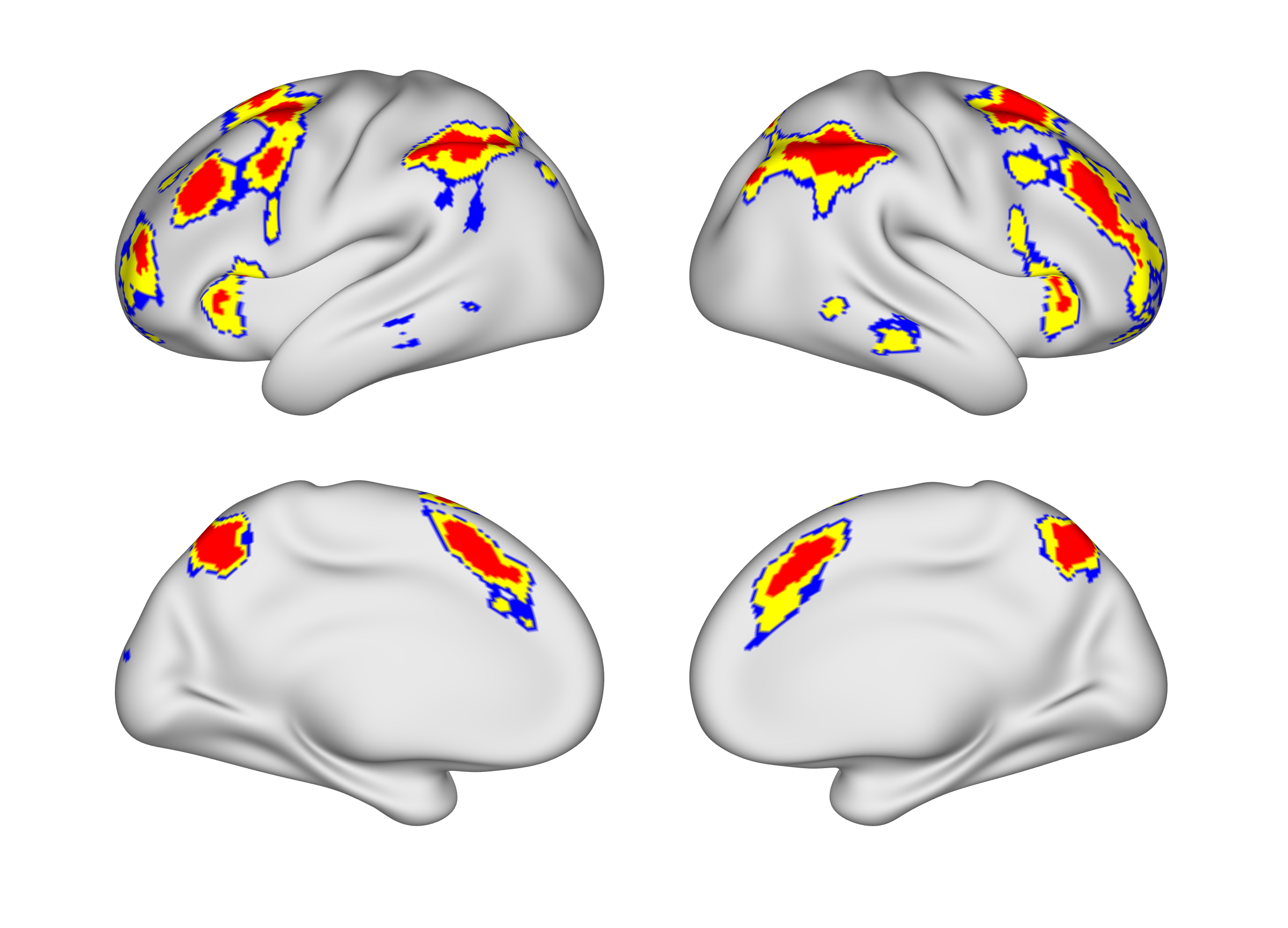
(a) Separate Method, $c=1.5$

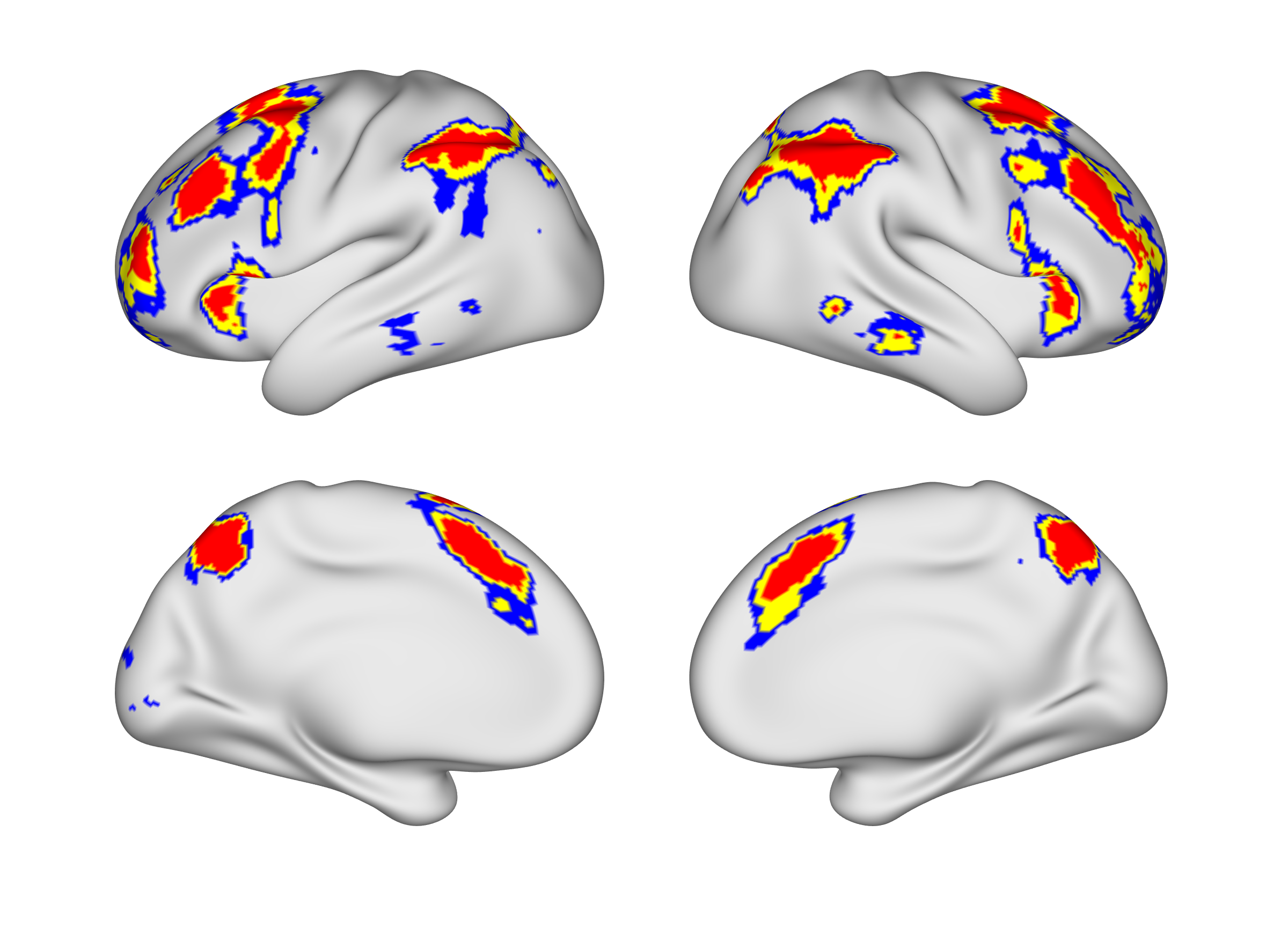
(b) Joint Method, $c=1.5$

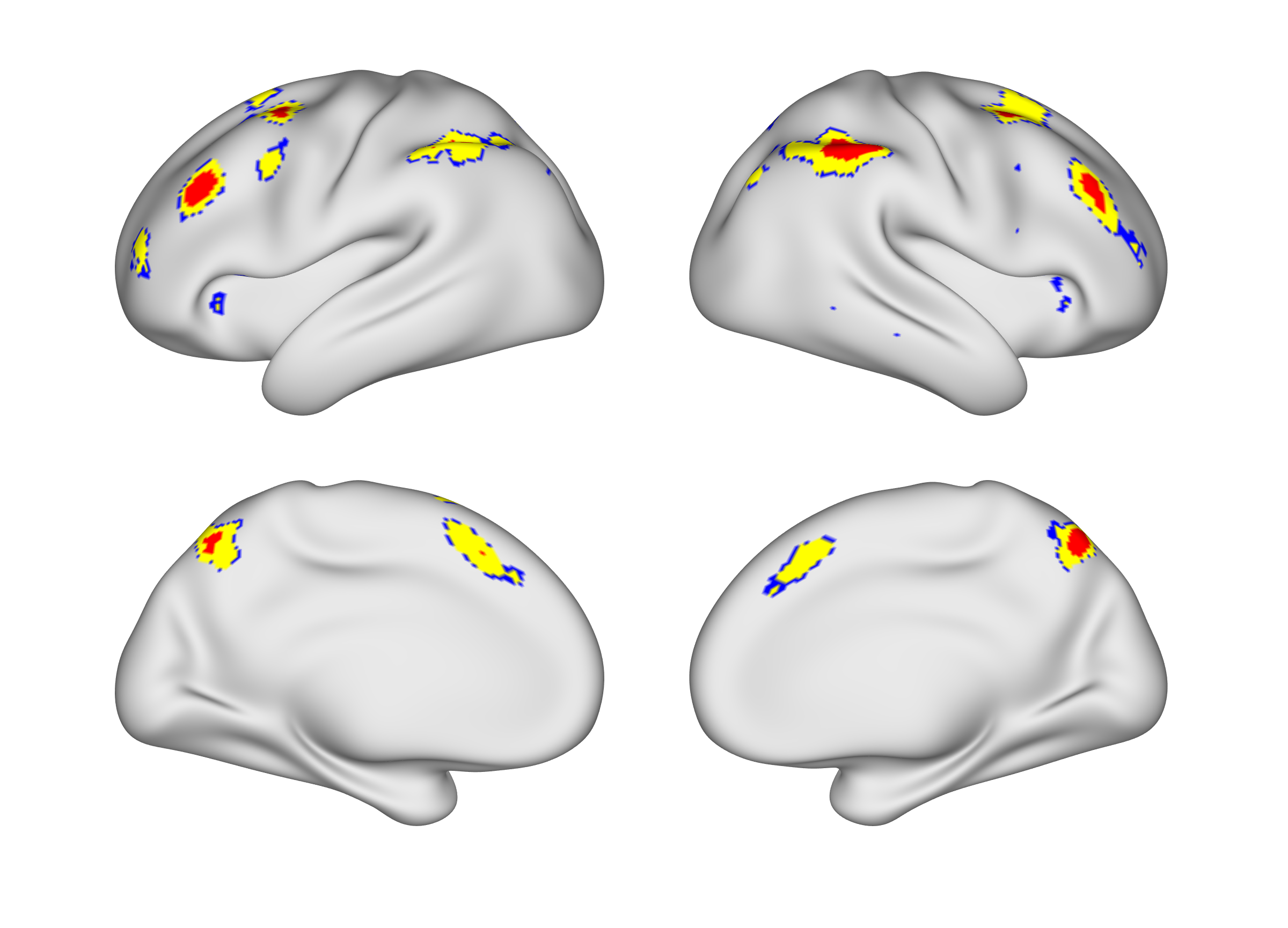
(c) Separate Method, $c=2.5$

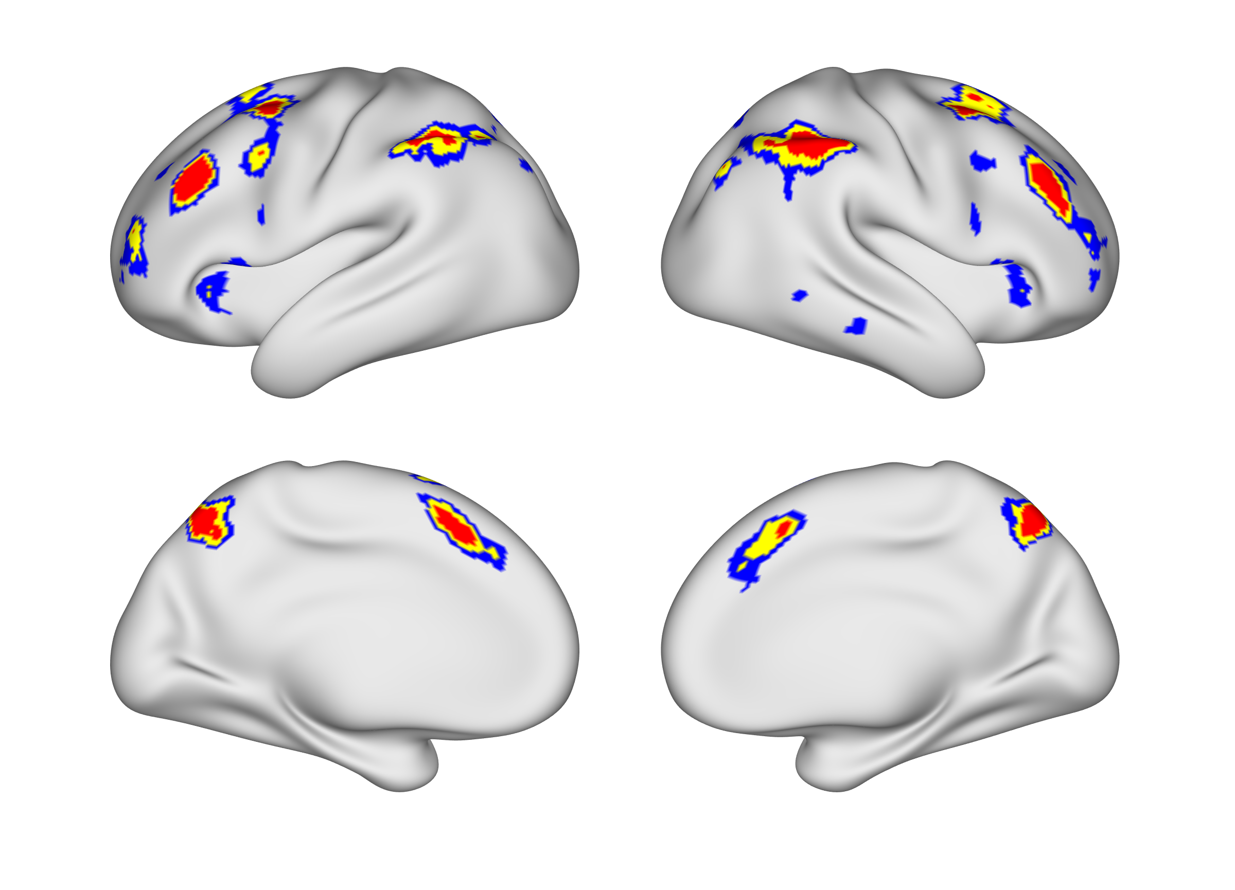
(d) Joint Method, $c=2.5$

Figure 1: An illustration of confidence regions, developed in this work, applied to task-based fMRI: red area denotes upper confidence region $\hat{\mathcal{A}_{c}^{+}}$, blue area denotes lower confidence region $\hat{\mathcal{A}_{c}^{-}}$, and the yellow area denotes the point estimate for the excursion set $\hat{\mathcal{A}_{c}}$. The rows differ in threshold $c$ in the % blood-oxygen-level-dependent (BOLD) change, and the columns differ in confidence region construction methods.

In this paper, we introduce testing-based confidence regions $\hat{\mathcal{A}}_{c}^{+}$ and $\hat{\mathcal{A}}_{c}^{-}$ which control the FDR over space in the upper and lower directions, respectively, with respect to the true excursion set $\mathcal{A}_{c}$. Our proposed approach uses one-sided testing at the level $c$, instead of the usual two-sided testing, which allows us to control directional errors. We investigate two modes of multiple testing for confidence region construction: one using the Benjamini-Hochberg procedure, and the other using a two-stage adaptive procedure proposed in [13]. This two-stage procedure is useful in increasing statistical power when the targeted excursion set is small, which occurs frequently for higher levels $c$. Testing in the positive and negative directions separately we obtain confidence sets for each direction. We continue by constructing confidence sets with joint error control over the two directions, in which the tests for the positive and negative directions are considered together in a single multiple testing procedure. An illustration of the separate and joint confidence regions in practice is presented in Figure 1. We evaluate the performance of the proposed methods in terms of FDR, for type-I error, and false non-discovery rate (FNDR), for type-II error, defined with respect to the excursion set.

The rest of the paper is organized as follows. In Section 2, we present the problem formally, define the error rates for separate error control, and present the algorithms for controlling them. In Section 3, this approach is extended to the joint error control over the two directions. In Section 4 we evaluate the performance of the methods via simulation. In Section 5, a real data application to task fMRI data from the Human Connectome Project working memory task is presented.

2 Confidence Regions with Separate Error Control

In this section, we introduce a spatial inference framework that controls the FDR separately through two one-sided tests. Upper and the lower confidence regions are defined via positive and negative one-sided hypothesis testing where the spatial FDR is controlled at level $\alpha$ separately for each test.

2.1 Upper Confidence Region

2.1.1 Construction

Given locations $v$ within a finite lattice $\mathcal{V}\subset\mathbb{R}^{D}$, we can construct an upper confidence region by testing in the positive direction at the level $c$. For each $v\in\mathcal{V}$, we consider the null and alternative hypotheses given by

$$H_{0}^{U}(v):\mu(v)\leq c\quad\mbox{vs.}\quad H_{A}^{U}(v):\mu(v)>c$$ (1)

at each location $v\in\mathcal{V}$ with corresponding null set $(\mathcal{A}_{c})^{C}\subseteq\mathcal{V}$, the complement of $\mathcal{A}_{c}$. To do so, let

$$t(v)=\frac{\hat{\mu}(v)-c}{\hat{\sigma}(v)/\sqrt{n}}$$

be the $t$-statistic for testing against the level $c$ as in (1) where $\hat{\mu}(v)$ and $\hat{\sigma}(v)$ are the point estimates of the true mean and standard deviation at each location $v\in\mathcal{V}$ respectively from $n$ i.i.d. samples. We can transform these test-statistics into a set of $p$-values, $\mathbf{p}^{U}=\left(p^{U}(1),\ldots,p^{U}(m)\right)$ to obtain an upper confidence region, at a given level $\alpha\in(0,1)$, by applying the Benjamini-Hochberg procedure [5, 9] as demonstrated in Algorithm 1.

Algorithm 1 Upper confidence region

1:$(t(v),\alpha)$

2: $\hat{\mathcal{A}}_{c}^{+}$

3:Obtain $m$ $p$-values $p^{U}{(v)}=1-F_{T_{n-1}}\left(t(v)\right),v=1,\ldots,m,$ where $F_{T_{n-1}}$ is the cdf of $t$-distribution with $n-1$ degrees of freedom from the positive one-sided test.

4:Apply the Benjamini-Hochberg procedure to the $p$-values $\mathbf{p}^{U}=\left(p^{U}(1),\ldots,p^{U}(m)\right)$ to get $p_{k}$, the threshold for rejection.

5:Define $\hat{\mathcal{A}}_{c}^{+}=\{v\in\mathcal{V}:p(v)\leq p_{k}\}$, the set of locations rejected.

6:Return the upper confidence region $\hat{\mathcal{A}}_{c}^{+}$.

The image space $\mathcal{V}$ can be naturally partitioned according to the rejection regions and the true non-null regions, see Table 1. For a given level $c$, the test and the corresponding regions can be visualized as shown in Figure 2.

Hypothesis	Not rejected	Rejected	Total
$H_{0}^{U}$	$(\mathcal{A}_{c})^{C}\cap(\hat{A}_{c}^{+})^{C}$	$(\mathcal{A}_{c})^{C}\cap\hat{\mathcal{A}}_{c}^{+}$	$(\mathcal{A}_{c})^{C}$
$H_{A}^{U}$	$\mathcal{A}_{c}\cap(\hat{\mathcal{A}}_{c}^{+})^{C}$	$\mathcal{A}_{c}\cap\hat{\mathcal{A}}_{c}^{+}$	$\mathcal{A}_{c}$
Total	$(\hat{\mathcal{A}}_{c}^{+})^{C}$	$\hat{\mathcal{A}}_{c}^{+}$	$\mathcal{V}$

Table 1: Partition of the image space $\mathcal{V}$ according to the ground truth and the rejection status (positive direction, one-sided). The color of the text in each cell corresponds to the color of the area in Figure 2 (b) and (c).

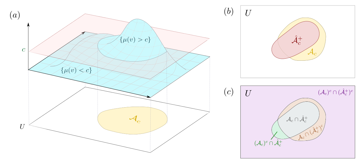
Figure 2: Upper confidence region schematic: (a) Example signal and the projection of the excursion set above $c$ ($\mathcal{A}_{c}$). (b) A hypothetical upper confidence region $\hat{\mathcal{A}}_{c}^{+}$ superimposed on the ground truth $\mathcal{A}_{c}$. (c) The division of (b) into regions corresponding to those specified in Table 1 as a visual representation of false positives (green) and false non-positives (orange).

2.1.2 Spatial FDR and FNDR

The false discovery proportion is given by the ratio of the number of true null locations rejected ($|(\mathcal{A}_{c})^{C}\cap\hat{\mathcal{A}}_{c}^{+}|=|\hat{\mathcal{A}}^{+}_{c}\setminus\mathcal{A}_{c}|$) to the number of all rejected locations ($|\hat{\mathcal{A}}^{+}_{c}|$)). The construction of $\hat{\mathcal{A}}_{c}^{+}$ ensures control of the upper spatial false discovery rate (${\rm FDR}_{U}$), which is defined as the expectation of the false discovery proportion, namely

$${\rm FDR}_{U}=\mathbb{E}\left[\frac{|\hat{\mathcal{A}}^{+}_{c}\setminus\mathcal{A}_{c}|}{|\hat{\mathcal{A}}^{+}_{c}|\vee 1}\right].$$ (2)

Algorithm 1 ensures that this is controlled in expectation to a level $\alpha$. Note that the p-values created this way satisfy the assumption of Positive Regression Dependency on each Subset (PRDS) [43], a necessary condition for application of the Benjamini-Hochberg procedure [9], which is considered reasonable for neuroimaging data [28].

In order to measure statistical power in Section 4, we shall use the false non-discovery proportion, which measures the ratio between the number of false non-discoveries and the number of total non-discoveries. Then, the upper false non-discovery rate (FNDR_U) is defined as

$${\rm FNDR}_{U}=\mathbb{E}\left[\frac{|\mathcal{A}_{c}\setminus\hat{\mathcal{A}}^{+}_{c}|}{|(\hat{\mathcal{A}}^{+}_{c})^{C}|\vee 1}\right],$$ (3)

where FNDR_U is the expected value of the false non-discovery proportion.

2.2 Lower Confidence Region

2.2.1 Construction

In order to construct a lower confidence region $\hat{\mathcal{A}_{c}^{-}}$ we consider testing against the negative one-sided null hypothesis at level $c$, defined as

$$H_{0}^{L}(v):\mu(v)\geq c\quad\mbox{vs.}\quad H_{A}^{L}(v):\mu(v)<c.$$ (4)

Construction of the lower confidence region is then formally given by Algorithm 2. This differs from Algorithm 1 in that it incorporates a two-stage adaptive procedure, as explained below.

Algorithm 2 Lower confidence region

1:$(t(v),\alpha)$

2: $\hat{\mathcal{A}}_{c}^{-}$

3:Obtain $m$ $p$-values $p^{L}{(v)}=F_{T_{n-1}}\left(t(v)\right)$ where $F_{T_{n-1}}$ is the cdf of $t$-distribution with $n-1$ degrees of freedom from the negative one-sided test.

4:Apply the two-stage adaptive procedure (Blanchard et al. [13]) to the $p$-values $\mathbf{p}^{L}=\left(p^{L}(1),\ldots,p^{L}(m)\right)$ to get $p_{k}$, the threshold for rejection.

5:Define $\hat{\mathcal{A}}_{c}^{-}=\{s\in S:p(s)\leq p_{k}\}^{C}$, the complement of the set of locations rejected.

6:Return the lower confidence region $\hat{\mathcal{A}}_{c}^{-}$.

Then, the null set corresponding to the hypothesis (4) is the closure $\mathcal{\underline{A}}_{c}$, defined as $\mathcal{\underline{A}}_{c}=\{v\in\mathcal{V}:\mu(v)\geq c\}$. Note that in order to test $\mu\geq c$ against $\mu<c$, we can instead test $-\mu\leq-c$ against $-\mu>-c$. Thus, the problem is symmetric and well defined in terms of the one-sided test in the negative side. The choice of formulation is dictated by the specific hypothesis constructed by the analysts.

Note here that unlike the case of the upper confidence region $\hat{\mathcal{A}_{c}^{+}}$, the lower confidence region $\hat{\mathcal{A}_{c}^{-}}$ now represents the non-significant set of locations. This asymmetry in the definition is by choice, stemming from the fact that while the null hypothesis in the negative direction is used in constructing $\hat{\mathcal{A}_{c}^{-}}$, the excursion set is still in the positive direction.

While having a similar construction procedure, the biggest difference between Algorithms 1 and 2 is that the latter uses an adaptive procedure to perform multiple testing. The BH procedure controls the FDR at $\alpha\cdot\pi_{0}$ level where $\pi_{0}\coloneqq\frac{m_{0}}{m}$ with $m$ being the total number of all the hypotheses, and $m_{0}$ being the number of true null hypotheses. When the fraction of true null hypotheses $\pi_{0}$ is small, as is typically the case in the test (4) for high values of $c$, the control of the FDR could be very conservative. This warrants an adaptive procedure that entails a correction on $\alpha\cdot\pi_{0}$ so that the actual error rate is kept at a higher (less conservative) level.

Various adaptive FDR control measures have been suggested, including Benjamini and Hochberg’s adaptive modification on the BH procedure [6] and others that followed [48, 49, 27, 39, 26, 38] under different assumptions on the data. We employ the two-stage adaptive procedure by Blanchard and Roquain (2009) [13] to form the lower confidence region. This works by estimating the number of null hypotheses in the first stage and using this information in a second stage to perform inference, see Section 2.2.3 for details.

The negative one-sided test partitions the image space $\mathcal{V}$ in the following way (Table 2). For a given level $c$, the test and the corresponding regions are visualized as shown in Figure 3.

Hypothesis	Not rejected	Rejected	Total
$H_{0}$	$\mathcal{\underline{A}}_{c}\cap\hat{\mathcal{A}}_{c}^{-}$	$\mathcal{\underline{A}}_{c}\cap(\hat{\mathcal{A}}_{c}^{-})^{C}$	$\mathcal{\underline{A}}_{c}$
$H_{A}$	$(\mathcal{\underline{A}}_{c})^{C}\cap\hat{\mathcal{A}}_{c}^{-}$	$(\mathcal{\underline{A}}_{c})^{C}\cap(\hat{\mathcal{A}}_{c}^{-})^{C}$	$(\mathcal{\underline{A}}_{c})^{C}$
Total	$\hat{\mathcal{A}}_{c}^{-}$	$(\hat{\mathcal{A}}_{c}^{-})^{C}$	$\mathcal{V}$

Table 2: Partition of the image space $\mathcal{V}$ according to the ground truth and the rejection status (negative direction, one-sided). The color of the text in each cell corresponds to the color of the area in Figure 3 (b) and (c).

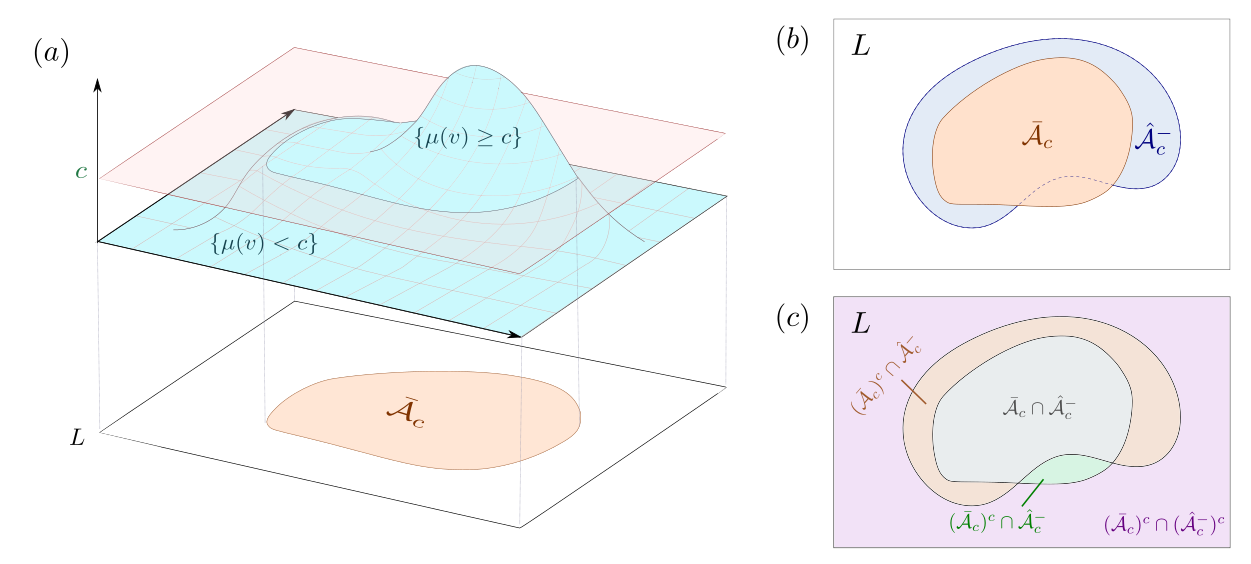
Figure 3: Lower confidence region schematic: (a) Example signal and the projection of the excursion set at and above $c$ ($\mathcal{\underline{A}}_{c}$). (b) A hypothetical lower confidence region $\hat{\mathcal{A}}_{c}^{-}$ superimposed on the ground truth $\mathcal{\underline{A}}_{c}$. (c) The division of (b) into regions corresponding to those specified in Table 2 as a visual representation of false positives (green) and false non-positives (orange).

2.2.2 Spatial FDR and FNDR

Similar to the upper regions, the lower false discovery proportion is measured by the number of true null locations rejected ($|\mathcal{\underline{A}}_{c}\cap(\hat{\mathcal{A}}_{c}^{-})^{C}|=|\mathcal{\underline{A}}_{c}\setminus\hat{\mathcal{A}}^{-}_{c}|$) divided by the number of rejected locations ($|(\hat{\mathcal{A}}^{-}_{c})^{c}|$) from the negative one-sided test. The false discovery rate for the lower confidence region (${\rm FDR}_{L}$) is defined as the expectation of of the false discovery proportion, namely

$${\rm FDR}_{L}=\mathbb{E}\left[\frac{|\mathcal{\underline{A}}_{c}\setminus\hat{\mathcal{A}}^{-}_{c}|}{|(\hat{\mathcal{A}}^{-}_{c})^{C}|\vee 1}\right].$$ (5)

The false non-discovery proportion is measured by the number of false null locations that are not rejected in the negative testing, $|(\mathcal{\underline{A}}_{c})^{C}\cap\hat{\mathcal{A}}_{c}^{-}|=|\hat{\mathcal{A}}^{-}_{c}\setminus\mathcal{\underline{A}}_{c}|$, divided by the number of all the non-rejected locations in the negative one-sided test, $|\hat{\mathcal{A}}^{-}_{c}|$. Again, the FNDR for the lower confidence region (${\rm FNDR}_{L}$) is defined as the expectation of the false non-discovery proportion,

$${\rm FNDR}_{L}=\mathbb{E}\left[\frac{|\hat{\mathcal{A}}^{-}_{c}\setminus\mathcal{\underline{A}}_{c}|}{|\hat{\mathcal{A}}^{-}_{c}|\vee 1}\right].$$ (6)

2.2.3 The Two-stage Adaptive Procedure

Here we provide formal details on the two-stage adaptive procedure by Blanchard and Roquain (2009) [13] used for our lower confidence region.

Two-stage adaptive procedures typically use the threshold collection of the form $\Delta_{i}=\pi^{-1}_{0}\frac{\beta(i)}{m}\cdot\alpha$. The weights $\beta(i)$ take the form $\beta(i)=\int_{0}^{i}u\,df(u)$ with $f$ being a fixed probability distribution on $(0,\infty)$ under unspecified dependence, or $\beta(i)=i$ under independence of the $p$-values or PRDS. By multiplying the threshold collection by a factor of $\pi^{-1}_{0}$, we expect to have less conservative procedure. In practice, we use $\Delta_{i}=\hat{\pi}_{0}^{-1}\frac{\beta(i)}{m}\cdot\alpha$ where $\hat{\pi}_{0}^{-1}=\frac{m}{\hat{m_{0}}}$ is an estimator of the true $\pi^{-1}_{0}$.

The two-stage adaptive procedure by Blanchard and Roquain [13] provably controls the FDR at the $\alpha$ level under positive dependence assumptions. In the first stage, a step-up procedure is conducted with threshold collection $\Delta_{i}=\frac{\beta(i)}{m}\alpha_{0}$ to get an estimate $\hat{m}_{0}=m-|R_{0}|$ where $|R_{0}|$ is the number of rejected hypotheses. In the second stage, an adaptive procedure is conducted with $\Delta_{i}=\hat{\pi}_{0}^{-1}\frac{\beta(i)}{m}\alpha_{1}$ where $\hat{\pi}_{0}^{-1}=F_{\kappa}(\frac{\hat{m_{0}}}{m})$. $F_{\kappa}(x)$ for $x\in[0,1]$ is given as follows:

$$F_{\kappa}(x)=\begin{cases}1,&\text{if }x\leq\kappa^{-1},\\ \frac{2\kappa^{-1}}{1-\sqrt{1-4(1-x)\kappa^{-1}}},&\text{otherwise}.\end{cases}$$

Blanchard and Roquain state that the two-stage procedure with $\alpha_{0}=\alpha/4,\alpha_{1}=\alpha/2$ and $\kappa=2$ produces less conservative FDR control compared to the linear step-up procedure alone (BH procedure) when $F_{\kappa=2}(\hat{m_{0}}/m)\geq 2$, which translates to when we expect at least $F_{2}^{-1}(2)=62.5\%$ of the tests to be rejected [13]. In the confidence region setting, the rejection corresponds to $(\hat{\mathcal{A}}^{-}_{c})^{C}$. When $c$ is high enough so that $(\hat{\mathcal{A}}^{-}_{c})^{C}$ is expected to be larger than $\hat{\mathcal{A}}^{-}_{c}$ (which is typically the case in neuroimaging inference), the two-stage adaptive procedure produces more powerful lower confidence regions.

3 Confidence Regions with Joint Error Control

In this section we develop upper and lower confidence regions which have joint (instead of separate) error rate control. To do so, we shall combine the directional $p$-values from the upper and lower direction tests into a single BH algorithm.

3.1 Hypothesis Testing

We now propose a confidence region construction procedure for jointly testing two null hypotheses:

$$H^{U}_{0}(v):\mu(v)\leq c\quad\mbox{vs.}\quad H^{U}_{A}(v):\mu(v)>c,$$ (7)

$$H^{L}_{0}(v):\mu(v)\geq c\quad\mbox{vs.}\quad H^{L}_{A}(v):\mu(v)<c,$$ (8)

where the superscripts $U$ and $L$ denote upper and lower respectively. Define $\mathcal{L}=\mathcal{V}\times\{-1\}$ and $\mathcal{U}=\mathcal{V}\times\{1\}$ to be two homeomorphic copies of $\mathcal{V}$. Given two sets $A,B\subseteq\mathcal{V}$, let $A\sqcup B:=A\times\{-1\}\cup B\times\{1\}$ refer to the disjoint union of the corresponding copies in $\mathcal{L}$ and $\mathcal{U}$, following the notation of [37]. Given this notation we can define the joint hypothesis space $\mathcal{H}=\mathcal{L}\sqcup\mathcal{U}$. The joint null set for the hypotheses is then $\mathcal{A}_{c}^{C}\sqcup\mathcal{\underline{A}}_{c}$. Considering the disjoint union will allow us to be able to provide joint confidence statements which hold for the upper and lower spaces simultaneously.

The space $\mathcal{V}$ is partitioned by the joint error control hypothesis testing framework as:

Hypothesis	Not Rejected	Rejected	Total
$H_{0}$	$\{(\mathcal{A}_{c})^{C}\cap(\mathcal{\hat{A}}_{c}^{+})^{C}\}\sqcup\newline \{\mathcal{\bar{A}}_{c}\cap\mathcal{\hat{A}}_{c}^{-}\}$	$\{(\mathcal{A}_{c})^{C}\cap\mathcal{\hat{A}}_{c}^{+}\}\sqcup\newline \{\mathcal{\bar{A}}_{c}\cap(\mathcal{\hat{A}}_{c}^{-})^{C}\}$	$(\mathcal{A}_{c})^{C}\sqcup\mathcal{\bar{A}}_{c}$
$H_{A}$	$\{\mathcal{A}_{c}\cap(\mathcal{\hat{A}}_{c}^{+})^{C}\}\sqcup\newline \{(\mathcal{\bar{A}}_{c})^{C}\cap\mathcal{\hat{A}}_{c}^{-}\}$	$\{\mathcal{A}_{c}\cap\mathcal{\hat{A}}_{c}^{+}\}\sqcup\newline \{(\mathcal{\bar{A}}_{c})^{C}\cap(\mathcal{\hat{A}}_{c}^{-})^{C}\}$	$\mathcal{A}_{c}\sqcup(\mathcal{\bar{A}}_{c})^{C}$
Total	$(\mathcal{\hat{A}}_{c}^{+})^{C}\sqcup\mathcal{\hat{A}}_{c}^{-}$	$\mathcal{\hat{A}}_{c}^{+}\sqcup(\mathcal{\hat{A}}_{c}^{-})^{C}$	$\mathcal{V}\times\{L,U\}$

Table 3: Table demonstrating the partition of $\mathcal{V}$ according to true hypothesis and rejection.

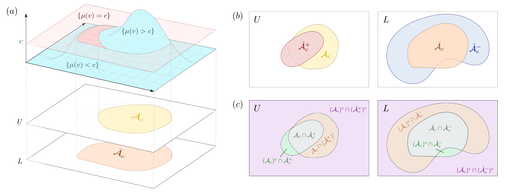
Figure 4: Upper and lower confidence regions from joint control method schematic: (a) Example signal and the projection of the excursion set above $c$ ($\mathcal{A}_{c}$) and at and above $c$ ($\mathcal{\bar{A}}_{c}$). (b) Hypothetical upper lower confidence regions $\hat{\mathcal{A}}_{c}^{+}$ and $\hat{\mathcal{A}}_{c}^{-}$ superimposed on the ground truth $\mathcal{A}_{c}$ and $\mathcal{\bar{A}}_{c}$ respectively. (c) The division of (b) into regions corresponding to those specified in Table 3 as a visual representation of false positives (green) and false non-positives (orange).

3.2 Joint Confidence Regions: Construction

Given the same setting of image space $\mathcal{V}$ consisting of $m$ locations, we construct the upper and lower confidence regions for the area above the threshold $c$, $\mathcal{A}_{c}$. Let $p^{U}(v)$ be the $p$-value calculated from the $t$-statistics corresponding to the positive test (7), and $p^{L}(v)=1-p^{U}(v)$ be the $p$-value calculated from the t-statistics corresponding to the negative test (8). Subsequently, $\mathbf{p}=\left(p^{L}(1),\ldots,p^{L}(m),p^{U}(1),\ldots,\ p^{U}(m)\right)$ collectively undergoes the BH procedure for joint FDR control through which the voxels are identified as rejected or not rejected.

Algorithm 3 Upper and Lower confidence regions with Joint Error Control

1:$(t(v),\alpha)$

2: $(\hat{\mathcal{A}}_{c}^{+},\hat{\mathcal{A}}_{c}^{-})$

3:Obtain $m$ $p$-values $p^{U}(v)=1-F_{T_{n-1}}\left(\left|t(v)\right|\right)$ where $F_{T_{n-1}}$ is the cdf of $t$-distribution with $n-1$ degrees of freedom.

4:Obtain $p^{L}(v)=1-p^{U}(v)$.

5:Apply the Benjamini-Hochberg procedure to $\mathbf{p}=\left(p^{L}(1),\ \ldots,\ p^{L}(m),\ p^{U}(1),\ \ldots,\ p^{U}(m)\right)$ to get $p_{k}$, the biggest p-value for rejection.

6:Define $\hat{\mathcal{A}}_{c}^{+}=\{v\in\mathcal{V}:p^{U}(v)\leq p_{k}\}$, the set of voxels rejected from $U$.

7:Define $\hat{\mathcal{A}}_{c}^{-}=\{v\in\mathcal{V}:p^{L}(v)\leq p_{k}\}^{C}$, the set of voxels rejected from $L$.

8:return the upper confidence region $\hat{\mathcal{A}}_{c}^{+}$ and the lower confidence region $\hat{\mathcal{A}}_{c}^{-}$.

Importantly the BH procedure controls the FDR to a level $\frac{m_{0}}{m}\cdot\alpha$ where $m$ denotes the number of locations tested, and $m_{0}$ denotes the true non-null locations [9]. With the joint error control hypothesis testing, the locations in the image are tested twice with each location being the true non-null hypothesis for at least one of the directions considered. This means that the FDR is effectively controlled at a level $\frac{m}{2m}\cdot\alpha$. We can take advantage of this and use a nominal level of $2\alpha$ instead of $\alpha$ while still providing FDR control at a level $\alpha$, leading to a substantial power improvement.

Technically PRDS does not hold for the jointly defined $p$-values due a limited amount of negative correlation between lower and upper $p$-values at the $\mathcal{A}_{c}$, however in practice this effect is very small and does not affect error control, as shown in Section 4.3.

3.3 Joint Confidence Regions: spatial FDR and FNDR

The false discovery proportion in confidence regions with joint FDR control is defined by the number of true null hypotheses that are rejected, $|\{(\mathcal{A}_{c})^{C}\cap\mathcal{\hat{A}}_{c}^{+}\}\sqcup\{\mathcal{\bar{A}}_{c}\cap(\mathcal{\hat{A}}_{c}^{-})^{C}\}|=|(\hat{\mathcal{A}}^{+}_{c}\setminus\mathcal{A}_{c})\sqcup(\mathcal{\underline{A}}_{c}\setminus\hat{\mathcal{A}}^{-}_{c})|$, divided by the total number of rejections across both one-sided tests, $|\hat{\mathcal{A}}^{+}_{c}\sqcup(\hat{\mathcal{A}}_{c}^{-})^{C}|$. The FDR for confidence regions with joint error rate control (${\rm FDR}_{J}$) is thus defined as the expected false discovery proportion,

$${\rm FDR}_{J}=\mathbb{E}\left[\frac{|(\hat{\mathcal{A}}^{+}_{c}\setminus\mathcal{A}_{c})\sqcup(\mathcal{\underline{A}}_{c}\setminus\hat{\mathcal{A}}^{-}_{c})|}{|\hat{\mathcal{A}}^{+}_{c}\sqcup(\hat{\mathcal{A}}_{c}^{-})^{C}|\vee 1}\right]=\mathbb{E}\left[\frac{|\hat{\mathcal{A}}^{+}_{c}\setminus\mathcal{A}_{c}|+|\mathcal{\underline{A}}_{c}\setminus\hat{\mathcal{A}}^{-}_{c}|}{(|\hat{\mathcal{A}}^{+}_{c}|+|(\hat{\mathcal{A}}_{c}^{-})^{C}|)\vee 1}\right].$$ (9)

Similarly, the false non-discovery proportion for joint FDR control is defined by the number of false non-discoveries over the upper and the lower sets $(|\{\mathcal{A}_{c}\cap(\mathcal{\hat{A}}_{c}^{+})^{C}\}\sqcup\{(\mathcal{\bar{A}}_{c})^{C}\cap\mathcal{\hat{A}}_{c}^{-}\}|=|(\mathcal{A}_{c}\setminus\hat{\mathcal{A}}^{+}_{c})\sqcup(\hat{\mathcal{A}}^{-}_{c}\setminus\mathcal{\underline{A}}_{c})|)$ and the number of total non-discoveries $(|(\mathcal{\hat{A}}_{c}^{+})^{C}\sqcup\mathcal{\hat{A}}_{c}^{-}|)$. Therefore, the FNDR for joint error control (${\rm FNDR}_{J}$) is defined as the expected false non-discovery proportion,

$${\rm FNDR}_{J}=\mathbb{E}\left[\frac{|(\mathcal{A}_{c}\setminus\hat{\mathcal{A}}^{+}_{c})\sqcup(\hat{\mathcal{A}}^{-}_{c}\setminus\mathcal{\underline{A}}_{c})|}{|(\mathcal{\hat{A}}_{c}^{+})^{C}\sqcup\mathcal{\hat{A}}_{c}^{-}|\vee 1}\right]=\mathbb{E}\left[\frac{|\mathcal{A}_{c}\setminus\hat{\mathcal{A}}^{+}_{c}|+|\hat{\mathcal{A}}^{-}_{c}\setminus\mathcal{\underline{A}}_{c}|}{(|(\hat{\mathcal{A}}^{+}_{c})^{C}|+|\hat{\mathcal{A}}^{-}_{c}|)\vee 1}\right].$$ (10)

Table 4 summarizes the spatial FDR and FNDR for the upper, lower and joint methods.

	FDR	FNDR
Separate Upper	$\mathbb{E}\left[\frac{|\hat{\mathcal{A}}^{+}_{c}\setminus\mathcal{A}_{c}|}{|\hat{\mathcal{A}}^{+}_{c}|\vee 1}\right]$	$\mathbb{E}\left[\frac{|\mathcal{A}_{c}\setminus\hat{\mathcal{A}}^{+}_{c}|}{|(\hat{\mathcal{A}}^{+}_{c})^{c}|\vee 1}\right]$
Separate Lower	$\mathbb{E}\left[\frac{|\mathcal{\underline{A}}_{c}\setminus\hat{\mathcal{A}}^{-}_{c}|)}{|(\hat{\mathcal{A}}^{-}_{c})^{C}|\vee 1}\right]$	$\mathbb{E}\left[\frac{|\hat{\mathcal{A}}^{-}_{c}\setminus\mathcal{\underline{A}}_{c}|}{|\hat{\mathcal{A}}^{-}_{c}|\vee 1}\right]$
Joint	$\mathbb{E}\left[\frac{|\hat{\mathcal{A}}^{+}_{c}\setminus\mathcal{A}_{c}|+|\mathcal{\underline{A}}_{c}\setminus\hat{\mathcal{A}}^{-}_{c}|}{(|\hat{\mathcal{A}}^{+}_{c}|+|(\hat{\mathcal{A}}_{c}^{-})^{C}|)\vee 1}\right]$	$\mathbb{E}\left[\frac{|\mathcal{A}_{c}\setminus\hat{\mathcal{A}}^{+}_{c}|+|\hat{\mathcal{A}}^{-}_{c}\setminus\mathcal{\underline{A}}_{c}|}{(|(\hat{\mathcal{A}}^{+}_{c})^{C}|+|\hat{\mathcal{A}}^{-}_{c}|)\vee 1}\right]$

Table 4: Summary of the spatial FDR and FNDR for confidence regions produced by different methods.

4 Simulations

4.1 Confidence Region Illustration

For the purpose of demonstrating the confidence regions, we apply the method to the 2-dimensional synthetic images $y_{i}$ of dimension $(50,50)$ with sample size 80 such that $y_{i}:\mathcal{V}\rightarrow\mathbb{R},i=1,\ldots,80$. The images $y_{i}$ are generated from three different signals in combination with noise field (Figure 5) in that $y_{i}(v)=\mu(v)+\epsilon_{i}(v)$ where $\mu(v)$ denotes the underlying signal function across voxels $v$, and $\epsilon_{i}(v)\sim\mathcal{N}(0,\sigma^{2})$ denotes the noise on top of the signal.

We consider three signals: ramp, circular, and step. The ramp signal increases linearly from -1 to 1 over 50 pixels horizontally where the ramp is repeated vertically, creating the pattern that increases from left to right of the image. The step signal is generated by smoothing over a 2D signal where the left half of the image is of value -1, and the right half of the image is of the value 1. The full width at half maximum (FWHM) used for smoothing the circle signal is 8 pixels. Note here that the ramp is invariant to and thus unaffected by different signal smoothing levels as it is defined as linearly gradual increase or decrease across the grid. The circle signal is generated by smoothing (FWHM 8 pixels) over a circle of radius 12 pixels which has magnitude 1 on the background of field of value -1. The noise field is obtained from smoothing the Gaussian random field $N(0,1.5^{2})$ by a kernel of FWHM 4. The noise field is scaled by the square root of the sum of squares of smoothing kernel to preserve the standard deviation.

Figure 5 shows the underlying signal images, and the 2D fields that are comprised of the underlying signals and the smoothed noise fields. Figure 6 shows the upper and the lower confidence regions superimposed on $\hat{\mathcal{A}}_{c}={v\in\mathcal{V}:\hat{\mu}(v)>c}$, where $\hat{\mu}(v)$ is the sample mean of the images. The confidence regions were constructed for the images presented in Figure 5, each with different error control (separate, and joint) methods.

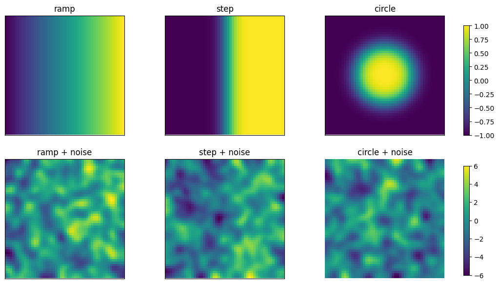
Figure 5: Synthetic images used for confidence region illustration. The first row shows ramp, step, and circle signals. The second row shows the same synthetic images with added smoothed Gaussian noise. The pixels in the noise field follows $N(0,1.5^{2})$, constituting an uncorrelated Gaussian noise field. The noise field is smoothed using FWHM 8 pixels.

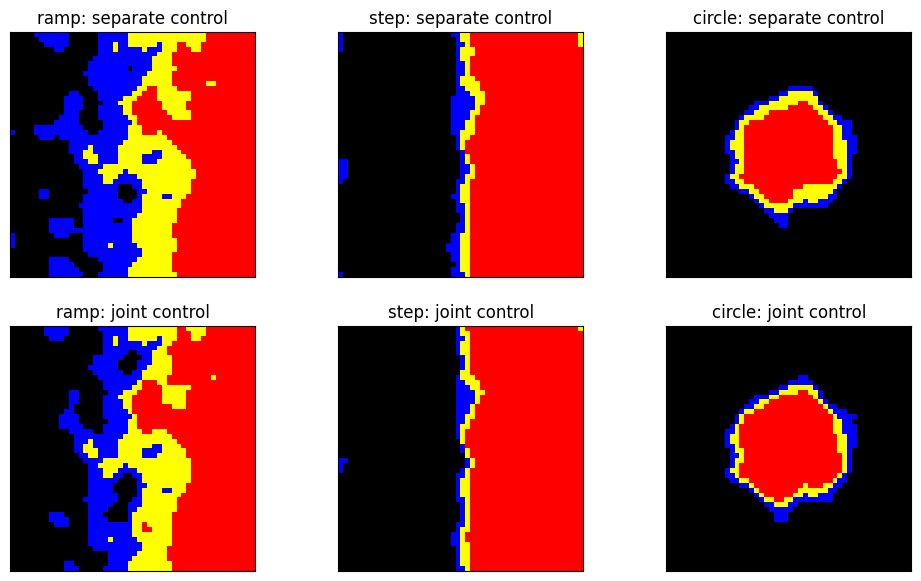
Figure 6: Confidence regions for the 2D synthetic images ($n=80$) with $\alpha=0.05$ for separate control, and $\alpha=0.1$ for the joint control; the red area denotes the upper confidence region $\hat{\mathcal{A}}_{c}^{+}$, the yellow area including the red area denotes the excursion set $\hat{\mathcal{A}}_{c}$, and the blue area including the yellow area denotes the lower confidence region $\hat{\mathcal{A}}_{c}^{-}$.

4.2 Error Rate Simulation

The error rate simulation was conducted to demonstrate the performance of the proposed confidence region methods in terms of empirical FDR and empirical FNDR depending on different $c$ levels. The simulation was repeated 1,000 times where in each simulation instance, a set of 80 synthetic 2D images were generated with each image consisting of 2500 voxels. Identical to the confidence region illustration, we denote each image as $y_{i}:\mathcal{V}\rightarrow\mathbb{R},i=1,\ldots,80$, where $y_{i}(v)=\mu(v)+\epsilon_{i}(v)$ for all the voxels $v$ in the image where $\mu(v)$ denotes the signal function, and $\epsilon_{i}(v)\sim\mathcal{N}(0,\sigma^{2})$ denotes the noise. The confidence regions were constructed via

1. joint error control for upper and lower confidence regions at $\alpha=0.1$,

2. separate error control for upper confidence region (BH procedure) at $\alpha=0.05$,

3. separate error control for lower confidence region (BH procedure) at $\alpha=0.05$, and

4. separate error control for lower confidence region (two-stage adaptive procedure) at $\alpha=0.05$.

Based on these four sets of confidence regions, false discovery and false non-discovery proportions were calculated at $c$ levels ranging from $-2$ to $2$ with 0.2 increments, resulting in 21 different $c$ levels in total. Empirical FDR and FNDR were then measured as the mean of the false discovery and false non-discovery proportions over 1,000 simulations at each $c$ level.

This process is repeated across different simulation settings generated using the combinations of three signals, three noise smoothing levels (${\rm FWHM}=0,5,10$), and three signal smoothing levels (${\rm FWHM}=5,10,15$). This resulted in 25 different simulation setting combinations, as only one signal smoothing level (no smoothing) was considered for the ramp signal. Among noise smoothing settings, only ${\rm FWHM}=5$ is reported, as the other two settings showed similar results.

The signals used for error simulation are identical to the signals in confidence region illustration (Figure 5) where the signal generation process is explained in detail.

There are some benefits for using ramp, step and circle signals for error simulation. ramp signal has gradual increase from $-1$ to $1$ from left to right with the values in the image having even distribution across $[-1,1]$. Thus, the ramp signal is effective in demonstrating how the error rates behave depending on different $c$ levels when there is linear change in slope in signal. The step signal has two flat regions, of value -1 on the first half and of value 1 on the second half, bridged by Gaussian kernel smoothing around 0 (${\rm FWHM}=8$). Step signals illustrates the effect of flat areas in the image on error rates. Finally, the circle signal is a variation on the step signal where the flat region of magnitude 1 is sloped out by Gaussian kernel (${\rm FWHM}=8$) smoothing over the background of value -1, creating a blob of flat region that resembles signals observed from fMRI scans.

Given the signals, noise fields are added on to the signal to create a synthetic image for simulation. The noise field is obtained from smoothing the Gaussian random field $N(0,1)$ with differing smoothness level to emulate correlated noise field assumption which is realistic and commonly observed in real world fMRI data.

For the step and circle fields, the simulation supposes three different signal smoothing levels (${\rm FWHM}=5,10,15$), and three different noise smoothing levels (${\rm FWHM}=0,5,10$). The ramp fields does not have differing signal smoothing levels as the ramp signal by generation is a gradation and thus does not include signal smoothing step, although the ramp fields still take different noise smoothing levels.

4.3 FDR

Signal	$\text{FWHM}=5$	$\text{FWHM}=10$	$\text{FWHM}=15$

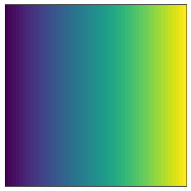
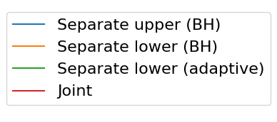
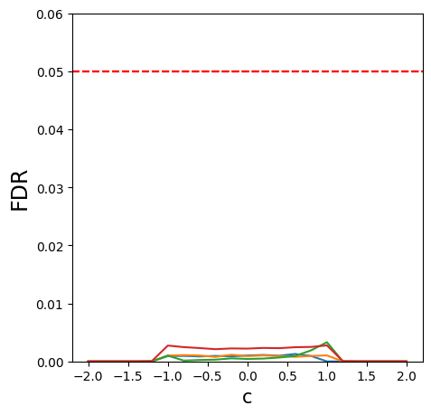
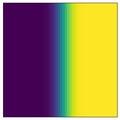
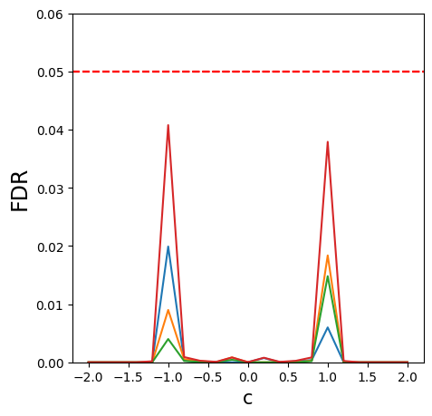
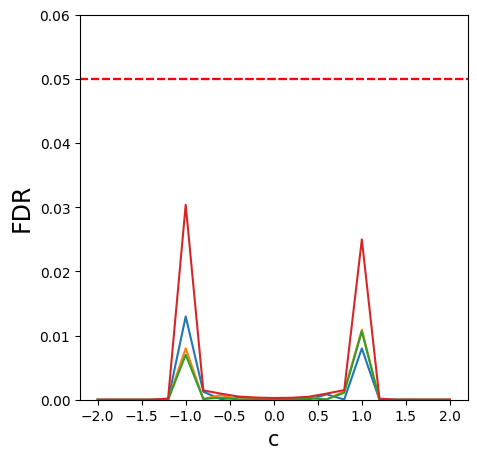
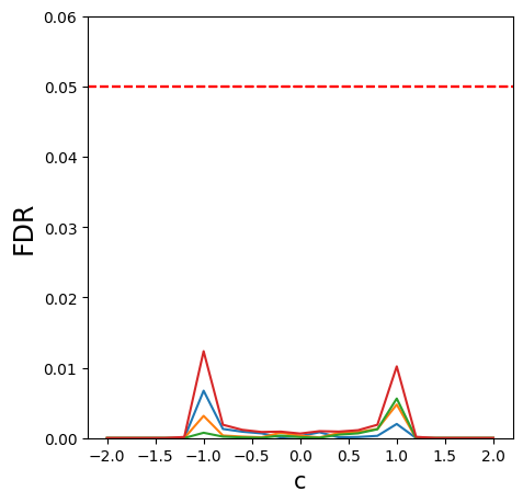
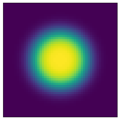
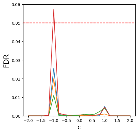
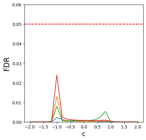
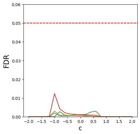
Figure 7: FDR simulation result for three signals (ramp, step and circle top to bottom) and three signal smoothing levels with noise smoothing at ${\rm FWHM}=5$. The $x$-axis denotes threshold $c$ ranging [-2, 2] with 0.2 increments. The $y$-axis denotes the empirical FDR. The red line denotes the joint method, the blue line the separate upper (BH), the yellow the separate lower (BH), and the green the separate lower (adaptive). The red dotted line signifies the nominal FDR level. Note here that the ramp signal has the same plots for different signal smoothing levels as they are unaffected by signal smoothing.

Figure 7 shows the empirical FDR change per different $c$ levels for each possible combination of smoothing levels and signals. The results for the entire simulation are presented in the supplementary materials. The threshold $c$ ranges from -2 to 2, increasing by 0.2 on the $x$-axis. The red line shows the empirical FDR change for the joint method, the blue line for the separate upper (BH), the yellow line for the separate lower (BH), and the green line for the separate lower (adaptive). For the ramp signal, the signal smoothing is non-existent, thus showing the same result for three different levels of signal smoothing.

The simulation results suggest that in general, the empirical FDR is effectively controlled under the 0.05 level across four methods and for all values of $c$. This is with an exception of the peak at $c=-1$ in circle signal with ${\rm FWHM}=5$ from the joint method. Although maintained below the 0.05 level, similar behaviour is observed at $c=-1$ and 1 for the step signal and $c=-1$ for the circle signal from the joint method. This is due to the fact that PRDS breaks down near the flat regions in the signals $c=1$ and $c=-1$ when using the joint method. See discussion for further details.

The asymmetry between the peaks at $c=-1$ and $c=1$ in circle signal joint method simulation is explained by the asymmetry in the number of pixels included in the area below 1 (the background) and above -1 (the circle). More voxels are rejected when testing for the lower side $H_{A}^{L}(v):\mu(v)<c$ with $c=1$ than when testing for the upper side $H_{A}^{U}(v):\mu(v)>c$ with $c=-1$. This leads to decreased denominator for the joint FDR at $c=-1$, while the other numbers involved in the calculation of joint FDR remain relatively insignificant, ultimately resulting in higher FDR at $c=-1$.

As predicted, the lower side adaptive method shows less conservative control of the FDR than the lower BH method in the circle signal images. This is in accordance with Blanchard and Roquain [13] which states that the proposed two-stage method works better when more tests are expected to be rejected which is equivalent to when there are more voxels below $c$ in the context of the negative one-sided test. This also explains why the lower side adaptive shows good control of the FDR when threshold is higher.

4.4 FNDR

Signal	$\text{FWHM}=5$	$\text{FWHM}=10$	$\text{FWHM}=15$

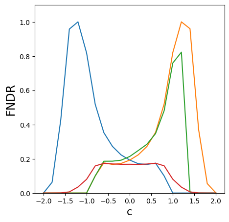
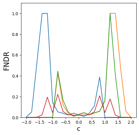
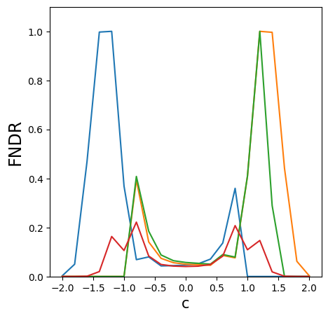
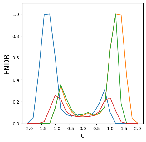
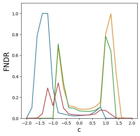
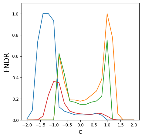
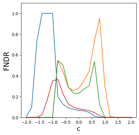
Figure 8: FNDR simulation result for three signals (ramp, step and circle top to bottom) and three signal smoothing levels with noise smoothing at ${\rm FWHM}=5$. The $x$-axis denotes threshold $c$ ranging [-2, 2] with 0.2 increments. The $y$-axis denotes the empirical FNDR. The red line denotes the joint method, the blue line the separate upper (BH), the yellow the separate lower (BH), and the green the separate lower (adaptive). Note here that the ramp signal has the same plots for different signal smoothing levels as they are unaffected by signal smoothing.

The simulation results for the empirical FNDR are presented in Figure 8 with the same simulation settings as the FDR.

Overall, the joint method shows consistently lower empirical FNDR compared to other methods. High peaks are displayed around the boundary values of $c\in(-2,-1)$ and $c\in(1,2)$ in signals for separate methods. This is because once the threshold is set too extreme, i.e. below -1 for the positive test or above 1 for the negative test, essentially all the voxels are supposed to be rejected with $\mathcal{A}_{c}$ being $\mathcal{V}$. Therefore, any non-rejected voxels due to noise are all false non-rejections. Since the noise is distributed $N(0,1)$, if the threshold is set too high or low, i.e. past -2 or 2, rarely are voxels falsely not-rejected due to the effect of very big or very small noise.

Much like the FDR simulation, the asymmetric pattern in the circle signal for joint method stems from the asymmetry in the number of voxels in the circle signal and the background. Otherwise, the pattern of empirical FNDR demonstrated by the step and circle signals are similar.

Generally, lower BH shows higher FNDR than lower adaptive as the threshold gets higher, signifying that the two-stage adaptive procedure exhibits a higher power than the BH procedure when more tests are expected to be rejected. As can be seen from Figure 8, signal smoothing does not bring as much improvement in power detection with the empirical FNDR plots, showing similar range of empirical FNDR values across different signal smoothing levels.

5 Human Connectome Project Data Application

5.1 The Human Connectome Project Data Description

The Human Connectome Project (HCP) is a five-year study which aims to map structual and functional human brain connectivity in young adults through multiple neuroimaging modalities [50]. In this section, we detail results of a real-data analysis performed on the HCP dataset with 77 participants using the confidence region methodologies proposed in this paper, as well as the method from SSS which refers to the bootstrap-based confidence region construction algorithm following Bowring (2019) [15] and SSS [41]. The confidence regions are built on the 77 subject-level contrast images from N-back working memory task comparing the 0-back vs. 2-back memory task. In the N-back working memory task, the participants are shown a sequence of pictures of objects and asked to remember them either immediately or 2 turns later. The image pre-processing details are presented in [29, 2].

5.2 Confidence Region Result

The $95\%$ confidence regions are constructed on fMRI scans from 77 subjects as a real data application of the proposed methods after applying additional smoothing with Gaussian kernel with FWHM $=2.25$ to match the results shown in Bowring (2019) [15]. Confidence regions using 1) the joint method with $\alpha=0.1$, 2) the separate method with BH adjustment for upper and lower side each with $\alpha=0.05$, 3) the separate method with BH adjustment for upper side and two-stage adaptive procedure for lower with $\alpha=0.05$, and 4) SSS ($\alpha=0.05$) were compared with threshold level 1.0%, 1.5%, and 2.0% Blood Oxygenation Level Dependent (BOLD) change. Joint control confidence regions are produced with $\alpha=0.1$ instead of 0.05 for the reasons mentioned in chapter 3.

Threshold	Joint	Separate (BH)	Separate (adaptive)	SSS
1.0%
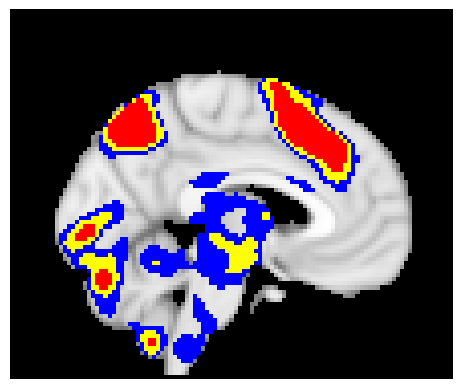
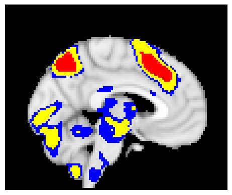
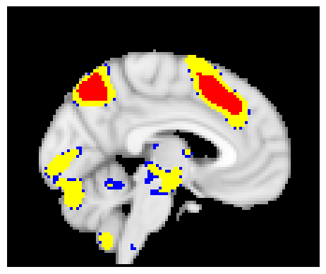
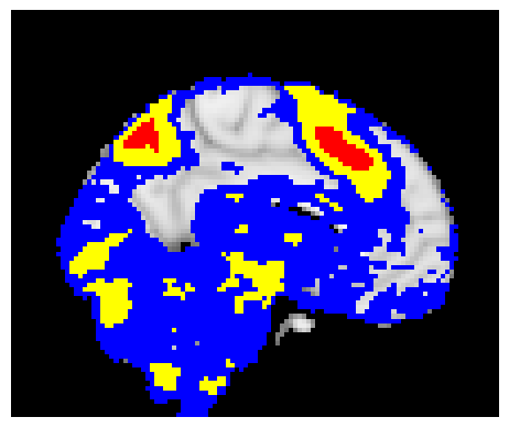
1.5%
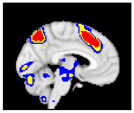
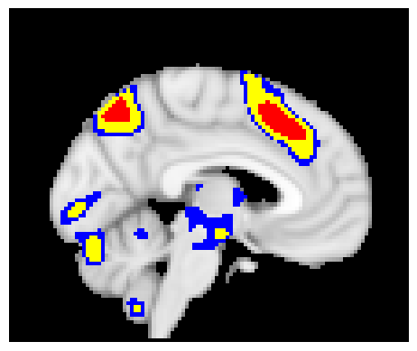
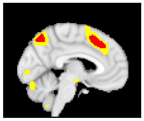
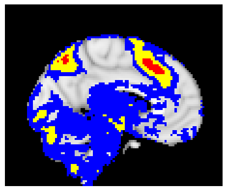
2.0%

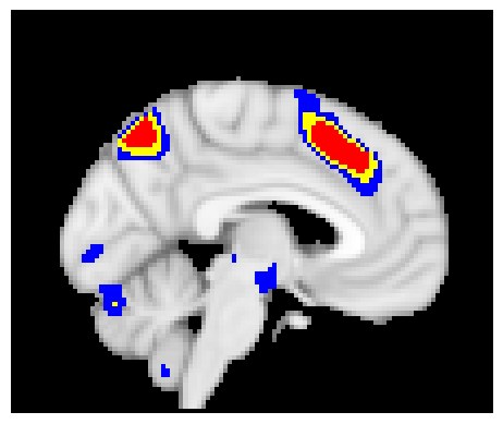
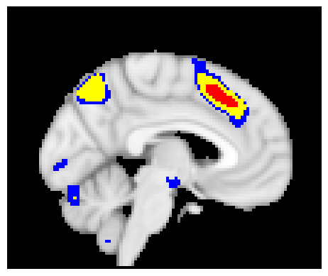
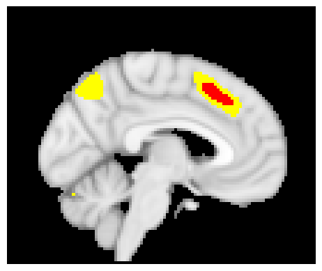
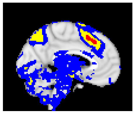
Figure 9: Confidence region application to the HCP data with 77 subjects in the sagittal slice view (X=-4, MNI space). The red area denotes the upper confidence region $\hat{\mathcal{A}}_{c}^{+}$, the yellow area including the red area denotes the excursion set $\hat{\mathcal{A}}_{c}$, and the blue area including the yellow area denotes the lower confidence region $\hat{\mathcal{A}}_{c}^{-}$. The rows differ in the threshold level $c$ by which the confidence regions are constructed. The columns denote different methods. Overall, FDR controlling hypothesis testing methods which are presented in the first three columns, show tighter spatial inference result when compared to SSS, thus providing a higher degree of localization and interpretability to the identified regions. The confidence regions show activation in areas such as the precuneus cortex, paracingulate gyrus, middle frontal gyrus, and angular gyrus which matches the expectation from the literature as areas involved in working memory.

Threshold	Joint	Separate (BH)	Separate (adaptive)	SSS
1.0%
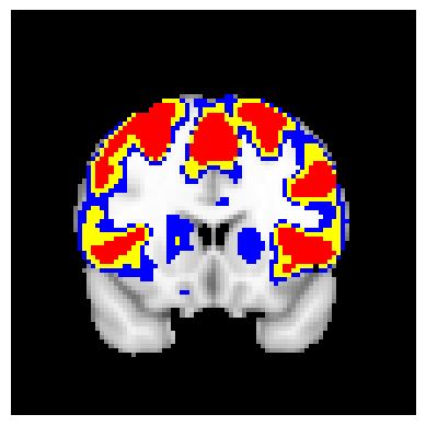
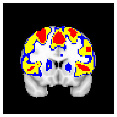
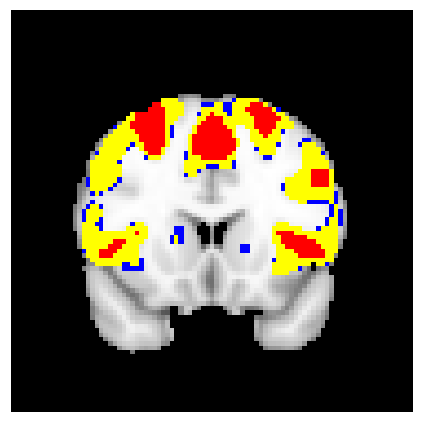
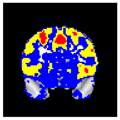
1.5%
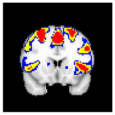
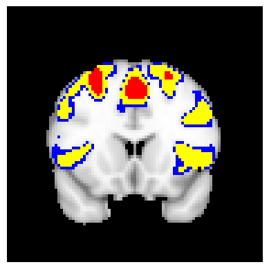
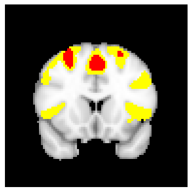
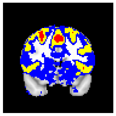
2.0%

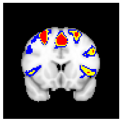
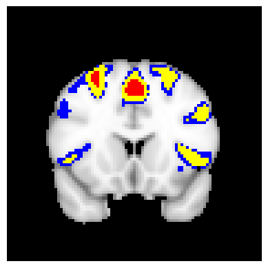
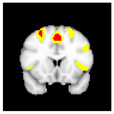
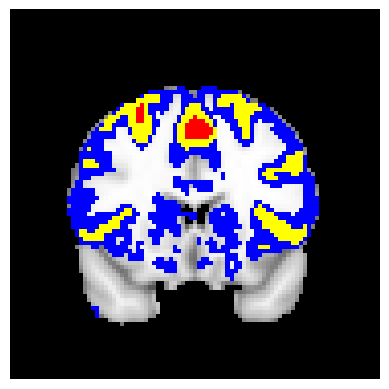
Figure 10: Confidence region application to the HCP data with 77 subjects in the coronal slice view (y=16, MNI space). The red area denotes the upper confidence region $\hat{\mathcal{A}}_{c}^{+}$, the yellow area including the red area denotes the excursion set $\hat{\mathcal{A}}_{c}$, and the blue area including the yellow area denotes the lower confidence region $\hat{\mathcal{A}}_{c}^{-}$. The rows differ in the threshold level $c$ by which the confidence regions are constructed. The columns denote different methods. Overall, FDR controlling hypothesis testing methods which are presented in the first three columns, show tighter spatial inference result when compared to SSS, thus providing a higher degree of localization and interpretability to the identified regions. The confidence regions show activation in areas such as the precuneus cortex, paracingulate gyrus, middle frontal gyrus, and angular gyrus which matches the expectation from the literature as areas involved in working memory.

Threshold	Joint	Separate (BH)	Separate (adaptive)	SSS
1.0%
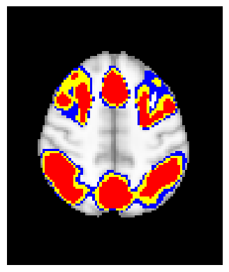
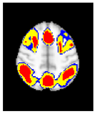
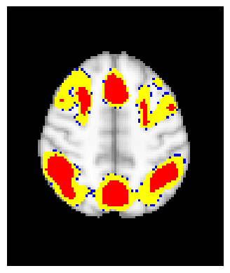
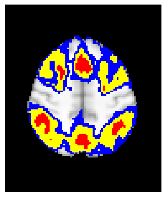
1.5%
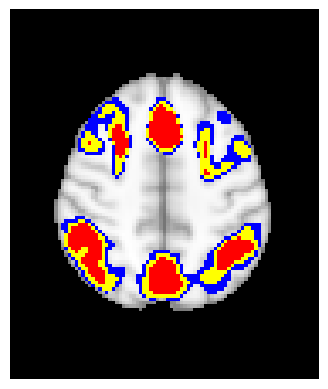
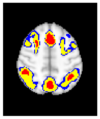
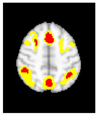
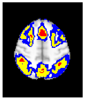
2.0%

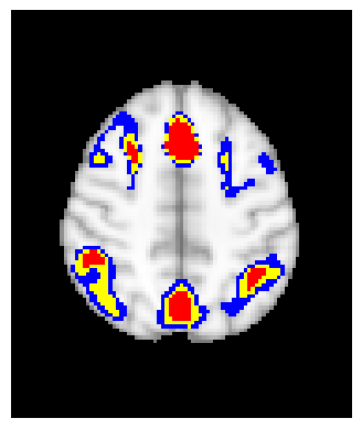
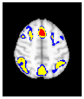
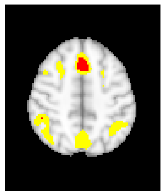
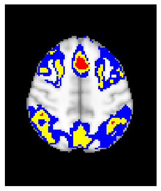
Figure 11: Confidence region application to the HCP data with 77 subjects in the axial slice view (Z=48, MNI space). The red area denotes the upper confidence region $\hat{\mathcal{A}}_{c}^{+}$, the yellow area including the red area denotes the excursion set $\hat{\mathcal{A}}_{c}$, and the blue area including the yellow area denotes the lower confidence region $\hat{\mathcal{A}}_{c}^{-}$. The rows differ in the threshold level $c$ by which the confidence regions are constructed. The columns denote different methods. Overall, FDR controlling hypothesis testing methods which are presented in the first three columns, show tighter spatial inference result when compared to SSS, thus providing a higher degree of localization and interpretability to the identified regions. The confidence regions show activation in areas such as the precuneus cortex, paracingulate gyrus, middle frontal gyrus, and angular gyrus which matches the expectation from the literature as areas involved in working memory.

For all slices, FDR controlling methods show tighter inference of both upper and lower CR compared to the SSS method. SSS shows smaller upper CR and larger lower CR which suggests more conservative inference compared to FDR controlling testing based methodologies. This is due to the fact that by controlling for FDR, the method allows for more false discoveries in exchange for more discoveries in general. Despite having higher $\alpha$ level at $0.1$, joint control confidence regions still show comparable results to other methods even with higher significance level. Naturally, as the threshold goes up, the area enclosed between the upper and lower confidence regions decreases.

Confidence regions with separate controls of FDR for lower and upper are presented in two forms for comparison: one with BH procedure for the lower confidence region, and the other one with the two-stage adaptive procedure for the lower confidence region. The upper confidence region remains the same as both methods uses BH procedure for the upper set FDR control. Lower confidence regions with adaptive method are smaller than lower sets with BH procedure which is to be expected as the two-stage adaptive procedure is less conservative when more voxels are thought to be rejected. In the context of negative one-sided testing, this is equivalent to when there are less number of voxels above $c$ than below $c$.

6 Conclusion and Discussion

This paper has developed upper and lower confidence regions for the excursion set $\mathcal{A}_{c}$, with spatial FDR control, based on directional hypothesis testing. These regions were constructed for separate upper and lower control and joint control over both directions. In order to boost power a two-stage adaptive approach was incorporated for the separate control and a natural adaption (using twice the desired $\alpha$ level whilst still controlling at the level $\alpha$) was used for the joint approach. Error rate simulations across a variety of scenarios showed that the empirical FDR was almost always controlled to the nominal level $\alpha=0.05$. Real data applications using fMRI data from the HCP showed that the confidence regions bounds were informative and particularly were more spatially precise than CRs obtained by existing methods [15, 41].

For the joint confidence regions, we use two one-sided tests rather than naively using a two-sided testing approach in which the hypothesis being tested is of the form

$$H_{0}(v):\mu(v)=c\quad\mbox{vs.}\quad H_{A}(v):\mu(v)\neq c.$$

At first glance naively testing against this null hypothesis and applying the BH might seem like a simpler approach for creating joint confidence regions. However, rejecting this null hypothesis does not provide directional error control, as the direction of the effect is not specified. Instead, testing against two one-sided null hypotheses (7 and 8) in the positive and the negative directions, as we do in our joint construction, allows us to provide directional inference.

For the confidence regions with separate error control, the FDR is controlled separately for the positive and negative directions. The joint confidence regions instead control the FDR simultaneously by considering both sets of directional nulls. Joint error control is theoretically more desirable than separate error control and the right choice of which to use may depend on the questions that users are trying to answer.

The two approaches are complementary and which to use depends on the error rate the analyst wishes to control. The separate control method is more informative, because it admits possibly different error rates in the upper and lower confidence regions. For example, when estimating a positive excursion set, the upper confidence region gives an indication of the minimal extent of the excursion set, whereas the lower confidence region gives an indication of the maximal extent of the excursion set, and controlling the error rate in one may be more important than in the other. The joint method is more concise in that it controls the FDR over the entire image, but it does not distinguish whether the errors occur in the upper confidence region or the lower confidence region. If the question of interest is one-directional in nature, using the separate method provides more informative confidence regions in terms of interpretability and error control.

In our simulations we observed that when the underlying signals in the data are thought to be relatively evenly distributed below and above the threshold $c$, the joint method usually provide less conservative confidence regions under the nominal $\alpha$ level (see e.g. the ramp and step signal simulation in Figure 7 first and second rows). Meanwhile, with the presence of signals with unbalanced distribution of areas below and above $c$, the lower confidence region with two-stage adaptive procedure provides better results (as signified by the circle signal simulation; c.f. Figure 7 third row). Most fMRI data would fall under this case.

A further observation of note is the presence of the peaks in the empirical FDR plots at $c=-1,1$ for the circle and step signals in Figure 7 . This can be attributed to the fact that PRDS, which is a sufficient condition involving positive dependency for the BH procedure to hold [9, 44], breaks down around $c=-1$ and 1 due to stronger negative dependency among the $p$-values for the lower and upper directions. The peaks of the FDR in Figure 7 are reduced in height with the presence of stronger signal smoothing as the gradients of the signal become less sharp.

Compared to SSS, the FDR-controlling method we propose in this work provides less conservative, thus tighter confidence regions. Aside from the power gain, the FDR-controlling framework based on hypothesis testing allows error control in finite samples, without requiring asymptotic assumptions.

As a closing note, we discuss potential extensions of this work. More immediate applications include the construction of the confidence regions for Cohen’s $d$ or $R^{2}$ in place of the mean values in the image [14, 1]. Testing based confidence regions easily extend to other correlation structures by combining it with other methods for correcting the FDR (e.g. [7, 9, 6]). Confidence regions could also be constructed in order to control other measures of error such as the false discovery proportion (FDP) [45, 20, 11] or in the context of selective inference on the hierarchies of hypotheses, such as the whole brain, regions, and individual voxels [3, 12, 45].

7 Acknowledgements

HR, AS and SD were partially supported by NIH grant R01MH128923. TMS, AS and SD were partially supported by NIH grant R01EB026859. Data were provided in part by the Human Connectome Project, WU-Minn Consortium (Principal Investigators: David Van Essen and Kamil Ugurbil; 1U54MH091657) funded by the 16 NIH Institutes and Centers that support the NIH Blueprint for Neuroscience Research; and by the McDonnell Center for Systems Neuroscience at Washington University.

8 Supplementary Materials

8.1 Simulation Results

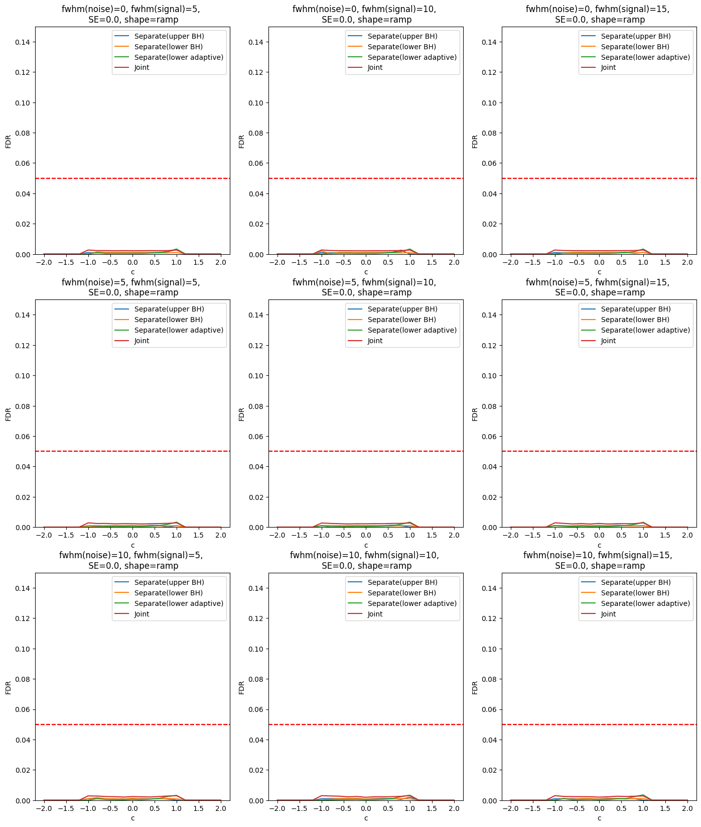
Figure 12: FDR simulation result for the ramp signal. The rows differ in noise smoothing (FWHM 0, 5, and 10) and the columns differ in signal smoothing levels (FWHM 5, 10, and 15). The $x$-axis denotes threshold c ranging [-2, 2] with 0.2 increments. The $y$-axis denotes the empirical FDR. The red line denotes the joint method, the blue line the separate upper (BH), the yellow the separate lower (BH), and the green the separate lower (adaptive). The red dotted line signifies the nominal FDR level.

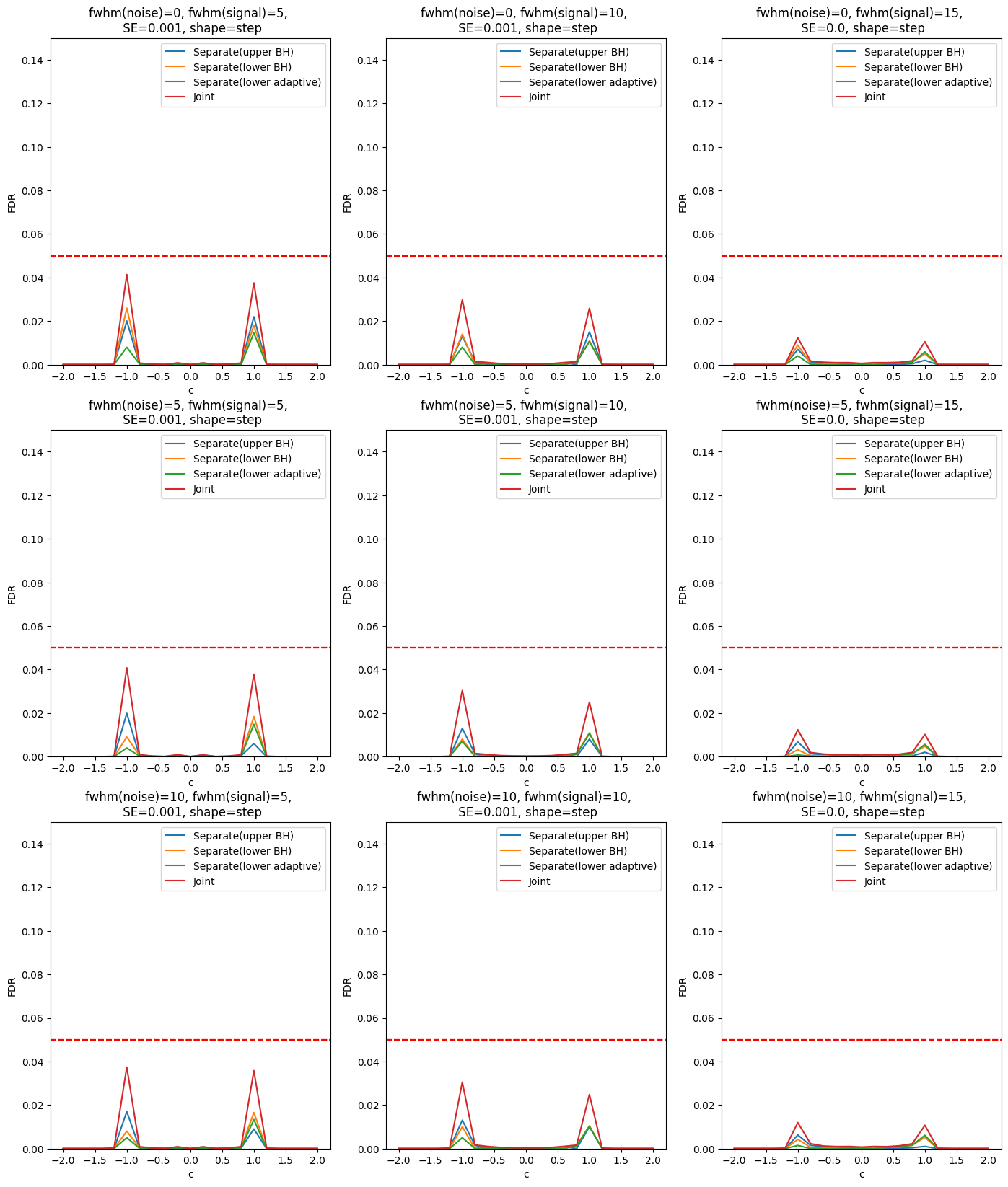
Figure 13: FDR simulation result for the step signal. The rows differ in noise smoothing (FWHM 0, 5, and 10) and the columns differ in signal smoothing levels (FWHM 5, 10, and 15). The $x$-axis denotes threshold c ranging [-2, 2] with 0.2 increments. The $y$-axis denotes the empirical FDR. The red line denotes the joint method, the blue line the separate upper (BH), the yellow the separate lower (BH), and the green the separate lower (adaptive). The red dotted line signifies the nominal FDR level.

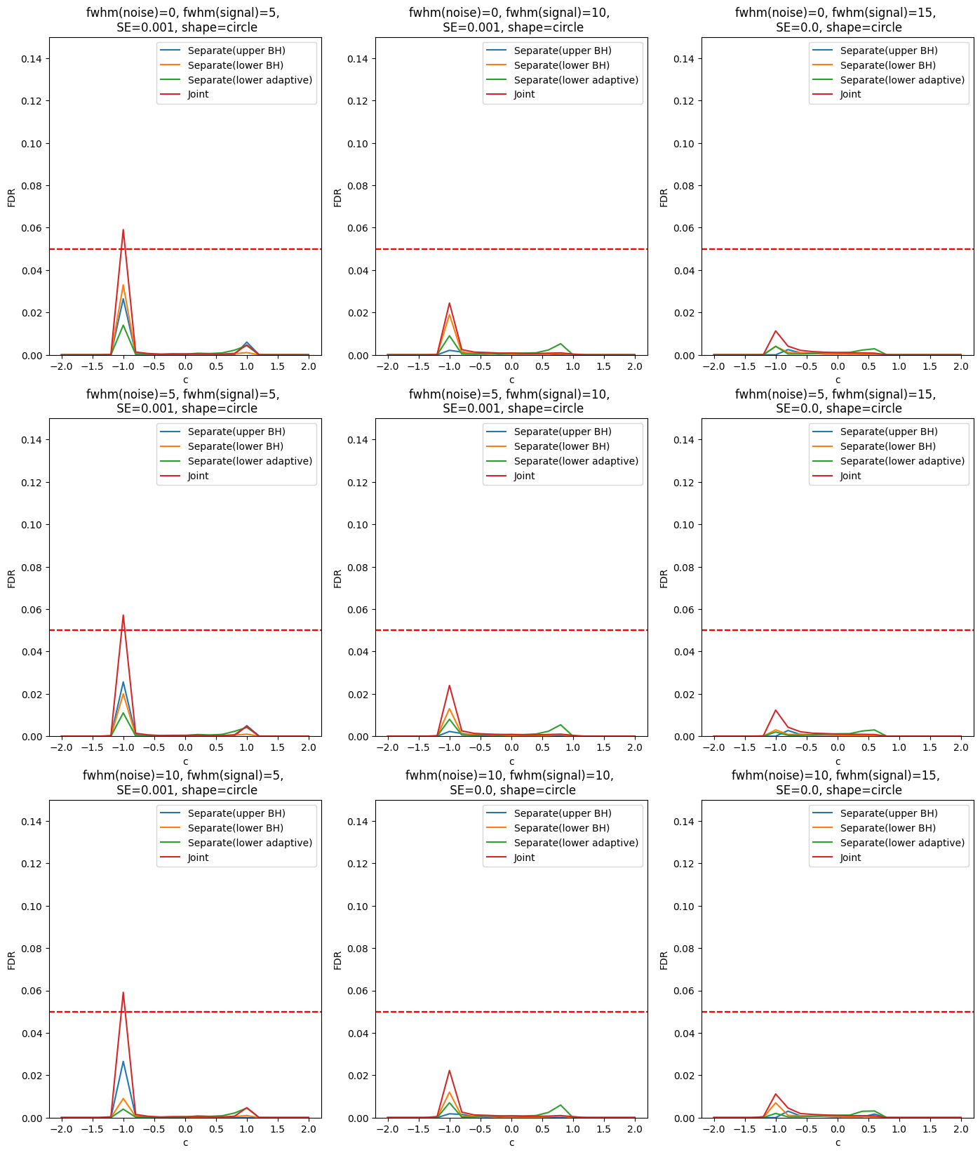
Figure 14: FDR simulation result for the circle signal. The rows differ in noise smoothing (FWHM 0, 5, and 10) and the columns differ in signal smoothing levels (FWHM 5, 10, and 15). The $x$-axis denotes threshold c ranging [-2, 2] with 0.2 increments. The $y$-axis denotes the empirical FDR. The red line denotes the joint method, the blue line the separate upper (BH), the yellow the separate lower (BH), and the green the separate lower (adaptive). The red dotted line signifies the nominal FDR level.

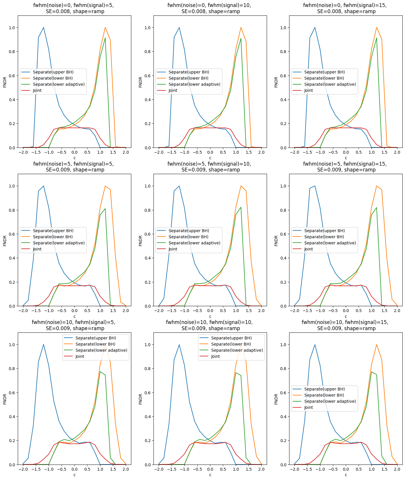
Figure 15: FNDR simulation result for the ramp signal. The rows differ in noise smoothing (FWHM 0, 5, and 10) and the columns differ in signal smoothing levels (FWHM 5, 10, and 15). The $x$-axis denotes threshold c ranging [-2, 2] with 0.2 increments. The $y$-axis denotes the empirical FNDR. The red line denotes the joint method, the blue line the separate upper (BH), the yellow the separate lower (BH), and the green the separate lower (adaptive).

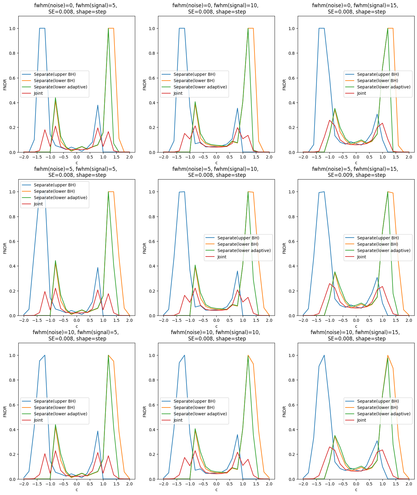
Figure 16: FNDR simulation result for the step signal. The rows differ in noise smoothing (FWHM 0, 5, and 10) and the columns differ in signal smoothing levels (FWHM 5, 10, and 15). The $x$-axis denotes threshold c ranging [-2, 2] with 0.2 increments. The $y$-axis denotes the empirical FNDR. The red line denotes the joint method, the blue line the separate upper (BH), the yellow the separate lower (BH), and the green the separate lower (adaptive).

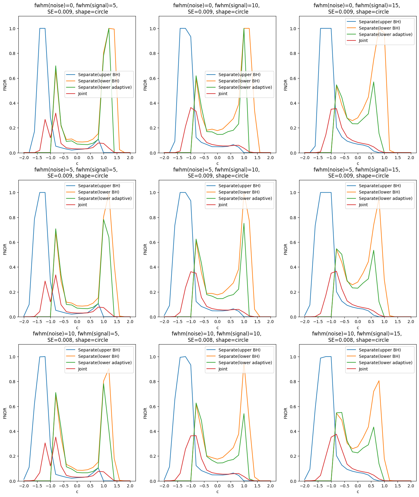
Figure 17: FNDR simulation result for the circle signal. The rows differ in noise smoothing (FWHM 0, 5, and 10) and the columns differ in signal smoothing levels (FWHM 5, 10, and 15). The $x$-axis denotes threshold c ranging [-2, 2] with 0.2 increments. The $y$-axis denotes the empirical FNDR. The red line denotes the joint method, the blue line the separate upper (BH), the yellow the separate lower (BH), and the green the separate lower (adaptive).

8.2 HCP Applications

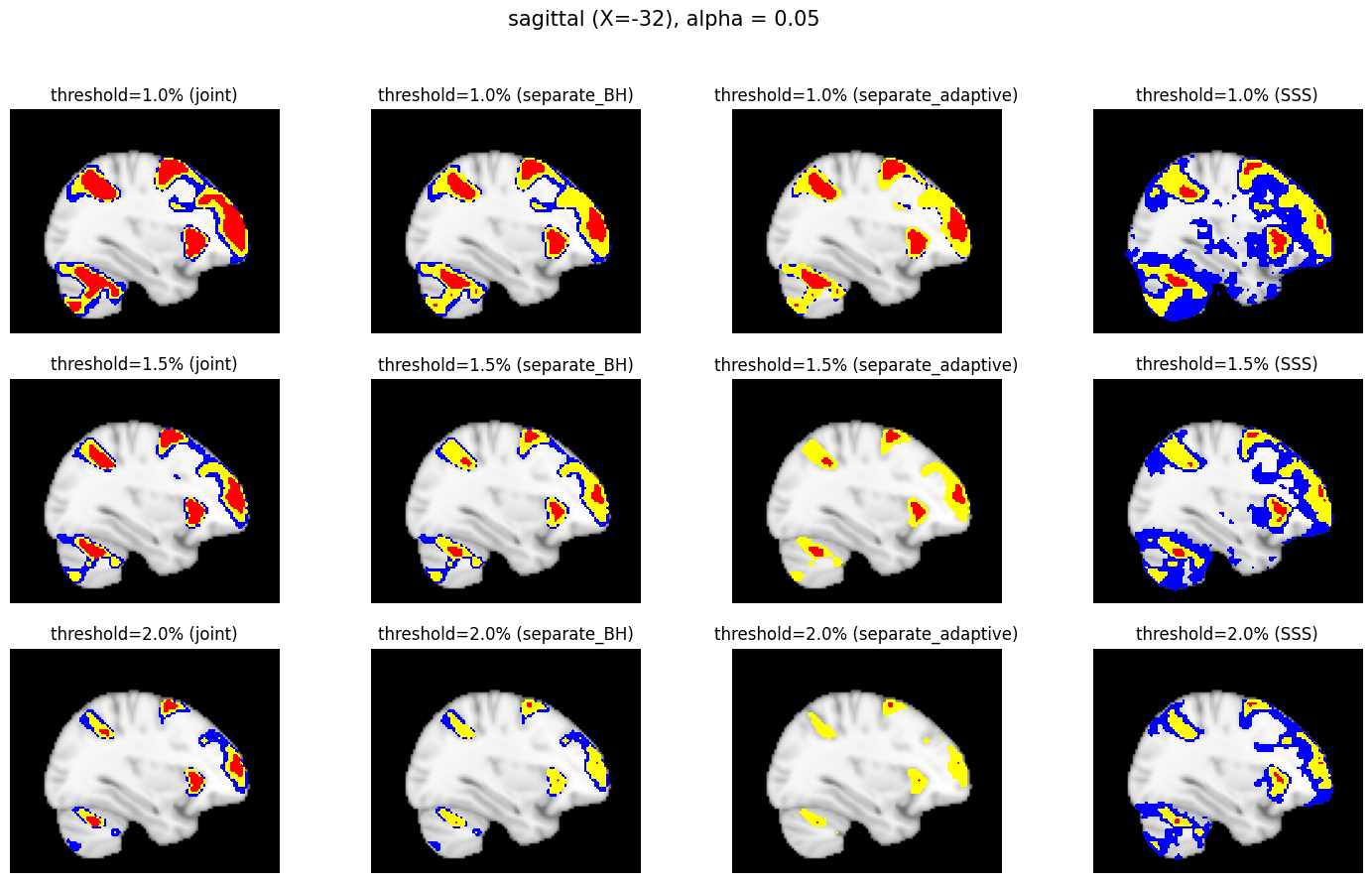
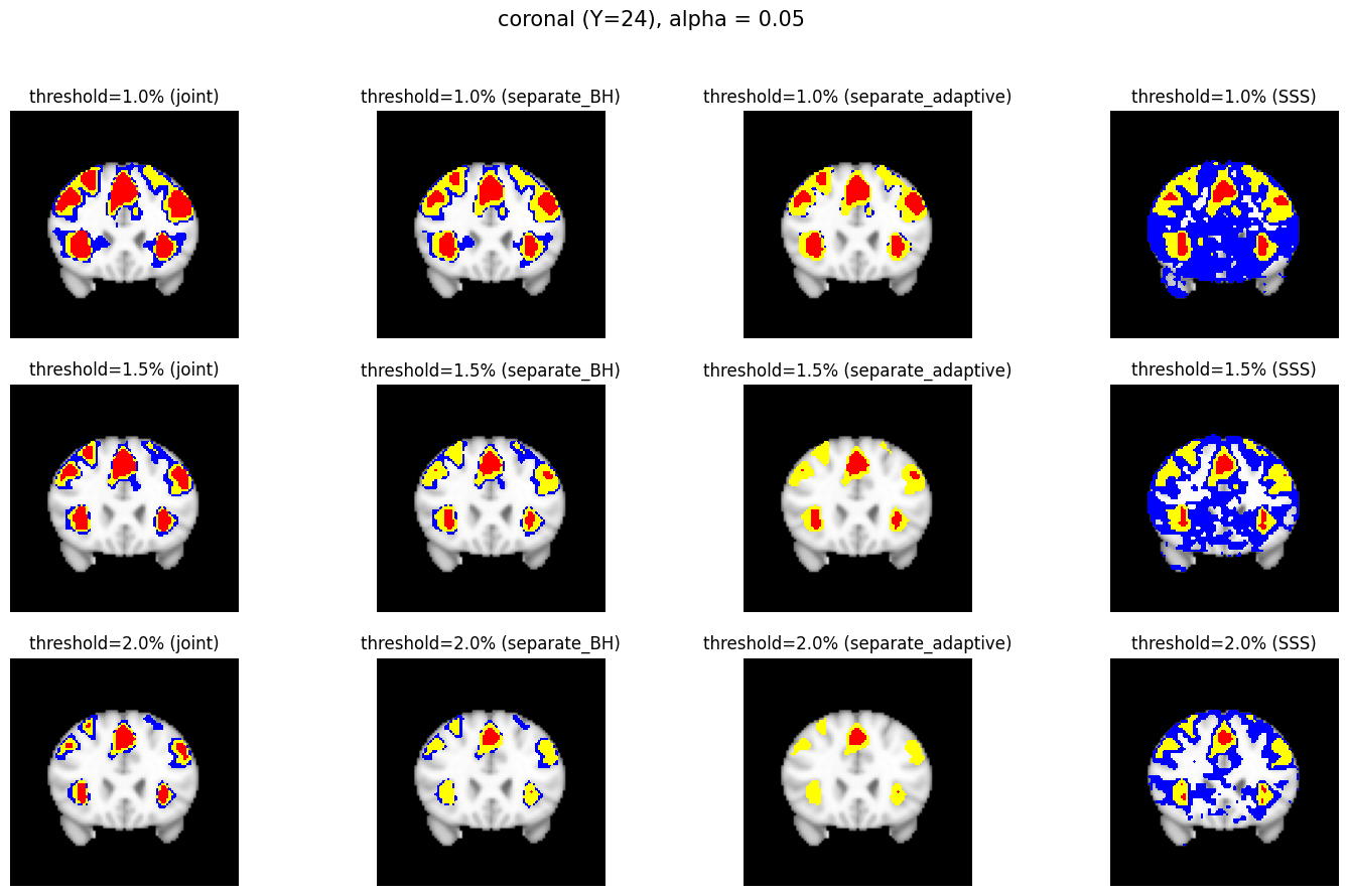
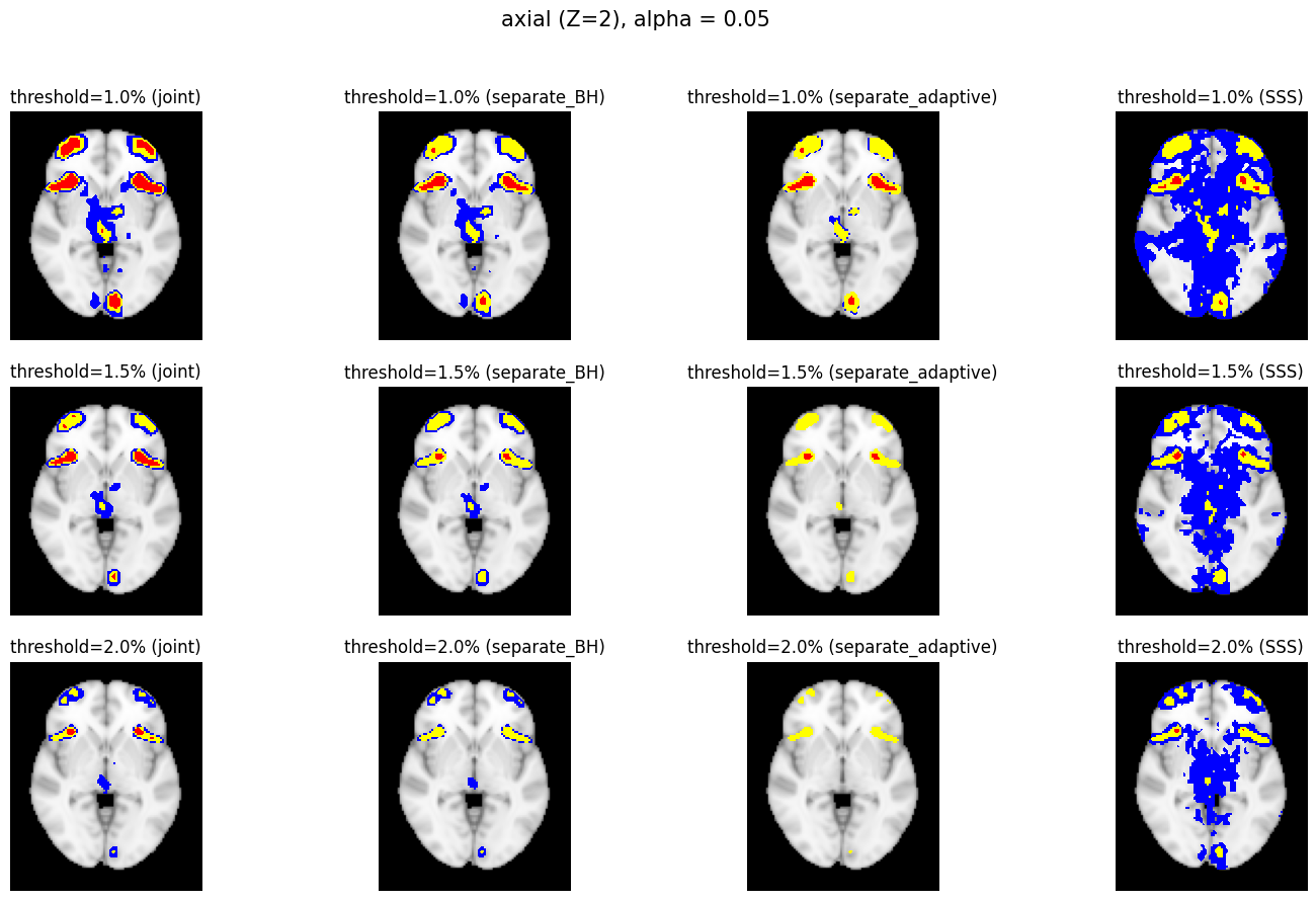
Figure 18: Confidence region application to the HCP data with 77 subjects in sagittal (X=-32), coronal (Y=24), and axial (Z=-2) from top to bottom. The red area denotes the upper confidence region $\hat{\mathcal{A}}_{c}^{+}$, the yellow area including the red area denotes the excursion set $\hat{\mathcal{A}}_{c}$, and the blue area including the yellow area denotes the lower confidence region $\hat{\mathcal{A}}_{c}^{-}$. The rows differ in the threshold level $c$ by which the confidence regions are constructed. The columns denote different methods. Overall, FDR controlling hypothesis testing methods which are presented in the first three columns, show tighter spatial inference result when compared to SSS, thus providing a higher degree of localization and interpretability to the identified regions. The confidence regions show activation in areas such as the precuneus cortex, paracingulate gyrus, middle frontal gyrus, and angular gyrus which matches the expectation from the literature as areas involved in working memory.

References

- [1] James Algina “A comparison of methods for constructing confidence intervals for the squared multiple correlation coefficient” In Multivariate Behavioral Research 34.4 Taylor & Francis, 1999, pp. 493–504
- [2] Deanna M Barch et al. “Function in the human connectome: task-fMRI and individual differences in behavior” In Neuroimage 80 Elsevier, 2013, pp. 169–189
- [3] Yoav Benjamini and Marina Bogomolov “Selective inference on multiple families of hypotheses” In Journal of the Royal Statistical Society Series B: Statistical Methodology 76.1 Oxford University Press, 2014, pp. 297–318
- [4] Yoav Benjamini and Ruth Heller “False discovery rates for spatial signals” In Journal of the American Statistical Association 102.480 Taylor & Francis, 2007, pp. 1272–1281
- [5] Yoav Benjamini and Yosef Hochberg “Controlling the false discovery rate: a practical and powerful approach to multiple testing” In Journal of the Royal statistical society: series B (Methodological) 57.1 Wiley Online Library, 1995, pp. 289–300
- [6] Yoav Benjamini and Yosef Hochberg “On the adaptive control of the false discovery rate in multiple testing with independent statistics” In Journal of educational and Behavioral Statistics 25.1 Sage Publications Sage CA: Los Angeles, CA, 2000, pp. 60–83
- [7] Yoav Benjamini, Abba M Krieger and Daniel Yekutieli “Adaptive linear step-up procedures that control the false discovery rate” In Biometrika 93.3 Oxford University Press, 2006, pp. 491–507
- [8] Yoav Benjamini and Daniel Yekutieli “False discovery rate–adjusted multiple confidence intervals for selected parameters” In Journal of the American Statistical Association 100.469 Taylor & Francis, 2005, pp. 71–81
- [9] Yoav Benjamini and Daniel Yekutieli “The control of the false discovery rate in multiple testing under dependency” In Annals of statistics JSTOR, 2001, pp. 1165–1188
- [10] Craig M Bennett, Michael B Miller and George L Wolford “Neural correlates of interspecies perspective taking in the post-mortem Atlantic Salmon: An argument for multiple comparisons correction” In Neuroimage 47.Suppl 1 Elsevier Science, 2009, pp. S125
- [11] Alexandre Blain, Bertrand Thirion and Pierre Neuvial “Notip: Non-parametric true discovery proportion control for brain imaging” In NeuroImage 260 Elsevier, 2022, pp. 119492
- [12] Gilles Blanchard, Pierre Neuvial and Etienne Roquain “Post hoc confidence bounds on false positives using reference families”, 2020
- [13] Gilles Blanchard and Etienne Roquain “Adaptive False Discovery Rate Control under Independence and Dependence.” In Journal of Machine Learning Research 10.12, 2009
- [14] Alexander Bowring, Fabian J.E. Telschow, Armin Schwartzman and Thomas E. Nichols “Confidence Sets for Cohen’s d effect size images” In NeuroImage 226, 2021, pp. 117477
- [15] Alexander Bowring, Fabian Telschow, Armin Schwartzman and Thomas E Nichols “Spatial confidence sets for raw effect size images” In NeuroImage 203 Elsevier, 2019, pp. 116187
- [16] Justin Chumbley, Keith Worsley, Guillaume Flandin and Karl Friston “Topological FDR for neuroimaging” In Neuroimage 49.4 Elsevier, 2010, pp. 3057–3064
- [17] Justin R Chumbley and Karl J Friston “False discovery rate revisited: FDR and topological inference using Gaussian random fields” In Neuroimage 44.1 Elsevier, 2009, pp. 62–70
- [18] Samuel Davenport and Thomas E Nichols “Selective peak inference: Unbiased estimation of raw and standardized effect size at local maxima” In NeuroImage 209 Elsevier, 2020, pp. 116375
- [19] Samuel Davenport, Thomas E Nichols and Armin Schwarzman “Confidence regions for the location of peaks of a smooth random field” In arXiv preprint arXiv:2208.00251, 2022
- [20] Samuel Davenport, Bertrand Thirion and Pierre Neuvial “FDP control in multivariate linear models using the bootstrap” In arXiv preprint arXiv:2208.13724, 2022
- [21] Samuel Davenport, Armin Schwarzman, Thomas E. Nichols and Fabian Telschow “Robust FWER control in neuroimaging using Random Field Theory: Riding the SuRF to continuous land Part 2”, 2023
- [22] Anders Eklund, Thomas E Nichols and Hans Knutsson “Cluster failure: Why fMRI inferences for spatial extent have inflated false-positive rates” In Proceedings of the national academy of sciences 113.28 National Acad Sciences, 2016, pp. 7900–7905
- [23] Helmut Finner “Stepwise multiple test procedures and control of directional errors” In The Annals of Statistics 27.1 Institute of Mathematical Statistics, 1999, pp. 274–289
- [24] Guillaume Flandin and Karl J Friston “Analysis of family-wise error rates in statistical parametric mapping using random field theory” In Human brain mapping 40.7 Wiley Online Library, 2019, pp. 2052–2054
- [25] Karl J Friston “Functional and effective connectivity in neuroimaging: a synthesis” In Human brain mapping 2.1-2 Wiley Online Library, 1994, pp. 56–78
- [26] Yulia Gavrilov, Yoav Benjamini and Sanat K Sarkar “An adaptive step-down procedure with proven FDR control under independence”, 2009
- [27] Christopher Genovese and Larry Wasserman “A stochastic process approach to false discovery control”, 2004
- [28] Christopher R Genovese, Nicole A Lazar and Thomas Nichols “Thresholding of statistical maps in functional neuroimaging using the false discovery rate” In Neuroimage 15.4 Elsevier, 2002, pp. 870–878
- [29] Matthew F Glasser et al. “The minimal preprocessing pipelines for the Human Connectome Project” In Neuroimage 80 Elsevier, 2013, pp. 105–124
- [30] Javier Gonzalez-Castillo et al. “Whole-brain, time-locked activation with simple tasks revealed using massive averaging and model-free analysis” In Proceedings of the National Academy of Sciences 109.14 National Acad Sciences, 2012, pp. 5487–5492
- [31] Wenge Guo and Joseph P Romano “On stepwise control of directional errors under independence and some dependence” In Journal of Statistical Planning and Inference 163 Elsevier, 2015, pp. 21–33
- [32] Wenge Guo, Sanat K Sarkar and Shyamal D Peddada “Controlling false discoveries in multidimensional directional decisions, with applications to gene expression data on ordered categories” In Biometrics 66.2 Oxford University Press, 2010, pp. 485–492
- [33] Satoru Hayasaka and Thomas E Nichols “Combining voxel intensity and cluster extent with permutation test framework” In Neuroimage 23.1 Elsevier, 2004, pp. 54–63
- [34] Satoru Hayasaka and Thomas E Nichols “Validating cluster size inference: random field and permutation methods” In Neuroimage 20.4 Elsevier, 2003, pp. 2343–2356
- [35] Satoru Hayasaka et al. “Nonstationary cluster-size inference with random field and permutation methods” In Neuroimage 22.2 Elsevier, 2004, pp. 676–687
- [36] Ruth Heller and Aldo Solari “Simultaneous directional inference” In Journal of the Royal Statistical Society Series B: Statistical Methodology Oxford University Press US, 2023, pp. qkad137
- [37] John Lee “Introduction to topological manifolds” Springer Science & Business Media, 2010
- [38] Dennis Leung and Ninh Tran “Adaptive procedures for directional false discovery rate control” In Electronic Journal of Statistics 18.1 The Institute of Mathematical Statisticsthe Bernoulli Society, 2024, pp. 706–741
- [39] Kun Liang and Dan Nettleton “Adaptive and dynamic adaptive procedures for false discovery rate control and estimation” In Journal of the Royal Statistical Society Series B: Statistical Methodology 74.1 Oxford University Press, 2012, pp. 163–182
- [40] T Maullin-Sapey, A Schwartzman and TE Nichols “Spatial confidence regions for combinations of excursion sets in image analysis: supplementary theory” In Journal of the Royal Statistical Society: Statistical Methodology Series B Oxford University Press, 2023
- [41] Stephan Sain Max Sommerfeld and Armin Schwartzman “Confidence Regions for Spatial Excursion Sets From Repeated Random Field Observations, With an Application to Climate” In Journal of the American Statistical Association 113.523 Taylor Francis, 2018, pp. 1327–1340
- [42] Thomas Nichols and Satoru Hayasaka “Controlling the familywise error rate in functional neuroimaging: a comparative review” In Statistical methods in medical research 12.5 Sage Publications Sage CA: Thousand Oaks, CA, 2003, pp. 419–446
- [43] Marco Perone Pacifico, Christopher Genovese, Isabella Verdinelli and Larry Wasserman “False discovery control for random fields” In Journal of the American Statistical Association 99.468 Taylor & Francis, 2004, pp. 1002–1014
- [44] E Roquain and G Blanchard “Two simple sufficient conditions for FDR control” In HAL 2008, 2008
- [45] Jonathan D Rosenblatt et al. “All-resolutions inference for brain imaging” In Neuroimage 181 Elsevier, 2018, pp. 786–796
- [46] William W Rozeboom “The fallacy of the null-hypothesis significance test.” In Psychological bulletin 57.5 American Psychological Association, 1960, pp. 416
- [47] Stephen M Smith and Thomas E Nichols “Threshold-free cluster enhancement: addressing problems of smoothing, threshold dependence and localisation in cluster inference” In Neuroimage 44.1 Elsevier, 2009, pp. 83–98
- [48] John D Storey “A direct approach to false discovery rates” In Journal of the Royal Statistical Society Series B: Statistical Methodology 64.3 Oxford University Press, 2002, pp. 479–498
- [49] John D Storey, Jonathan E Taylor and David Siegmund “Strong control, conservative point estimation and simultaneous conservative consistency of false discovery rates: a unified approach” In Journal of the Royal Statistical Society Series B: Statistical Methodology 66.1 Oxford University Press, 2004, pp. 187–205
- [50] David C Van Essen et al. “The Human Connectome Project: a data acquisition perspective” In Neuroimage 62.4 Elsevier, 2012, pp. 2222–2231
- [51] Asaf Weinstein, William Fithian and Yoav Benjamini “Selection adjusted confidence intervals with more power to determine the sign” In Journal of the American Statistical Association 108.501 Taylor & Francis, 2013, pp. 165–176
- [52] Anderson M Winkler, Paul A Taylor, Thomas E Nichols and Chris Rorden “False Discovery Rate and Localizing Power” In arXiv preprint arXiv:2401.03554, 2024
- [53] Keith J Worsley, Alan C Evans, Sean Marrett and P Neelin “A three-dimensional statistical analysis for CBF activation studies in human brain” In Journal of Cerebral Blood Flow & Metabolism 12.6 SAGE Publications Sage UK: London, England, 1992, pp. 900–918
- [54] Daniel Yekutieli and Yoav Benjamini “Resampling-based false discovery rate controlling multiple test procedures for correlated test statistics” In Journal of Statistical Planning and Inference 82.1-2 Elsevier, 1999, pp. 171–196
- [55] Hui Zhang, Thomas E. Nichols and Timothy D. Johnson “Cluster mass inference via random field theory” In NeuroImage 44.1, 2009, pp. 51–61