CEERS: Forging the First Dust Grains in the Universe?

Abstract

Context.

Aims.

Methods. This paper investigates the coevolution of metals and dust for 173 galaxies at $4.0<z\leq 11.4$ observed with JWST/NIRSpec in the CEERS project. We focus on galaxies with extremely low dust attenuation to understand the physical mechanisms at play.

Results. We developed a new version of the CIGALE code that integrates spectroscopic and photometric data. By statistically comparing observations with modeled spectra, we derive physical parameters to constrain these mechanisms.

Conclusions. Our analysis reveals a population of 49 extremely low dust attenuation galaxies (GELDAs), consistent with $A_{\mathrm{FUV}}=0.0$ within $2\sigma$ and $M_{\star}<10^{9}\,M_{\odot}$. The stacked spectrum of GELDAs shows a very blue UV slope $\beta_{\mathrm{FUV}}=-2.451\pm 0.066$ and a Balmer decrement H$\alpha$/H$\beta=2.932\pm 0.660$, consistent with no dust and Case B recombination with minimal underlying absorption. Notably, GELDAs are more prevalent at $z>8.8$ (83.3%) than at lower redshifts (26.3%), suggesting they could dominate in the early Universe. Using a far-infrared dust spectrum from the ALPINE sample, we study $M_{\mathrm{dust}}$ vs. $M_{\star}$ trends. These exhibit upper and lower sequences connected by transitional galaxies. Our comparison with models indicates a critical transition around $M_{\star}\approx 10^{8.5}\,M_{\odot}$, from dust dominated by stellar sources (SNe and AGB stars) to dust growth via gas accretion. This corresponds to a metallicity of $12+\log_{10}(\mathrm{O}/\mathrm{H})=7.60$ ($Z/Z_{\odot}\approx 0.1$), aligning with the point where ISM dust growth matches stellar dust production. The sample has a high gas fraction ($f_{\mathrm{gas}}\gtrsim 0.9$), with no significant gas expulsion, and high surface gas densities. This leads to low star formation efficiencies compared to sub-millimeter galaxies. GELDAs may help explain the observed excess of bright galaxies at $z\gtrsim 9$.

1 Introduction

After the big bang, nucleosynthesis started in the first stellar population formed in the Universe: population III stars (pop. III), and shortly after pop. II stars. Type II supernovae (SNae II) expelled metals much earlier than asymptotic giant branch (AGB) stars in the early Universe (Valiante et al. 2009; Hirashita et al. 2014; Dell’Agli et al. 2019; Walter et al. 2020), which then led to the formation of the first dust grains by coalescence of these metals (e.g. Schneider+24). Dust affects ultraviolet (UV) and optical emissions through dust attenuation and reddening. Dust IR emission is a major cooling agent. This energy warms dust and is re-emitted at infrared (IR) and sub-millimeter (sub-mm) wavelengths (Burgarella2005, Malek2018, Pozzi2021). Dust plays a critical role in the formation of low-mass stars by facilitating several key processes in the interstellar medium (ISM). Molecular hydrogen (H₂), which is essential for cloud collapse and subsequent star formation, does not form efficiently in the gas phase under typical ISM conditions. Instead, H₂ formation is catalyzed on the surfaces of dust grains, making dust indispensable to initiating star formation even at warm temperatures (Grieco et al. 2023). Once formed, these grains can act as seeds for further grain growth in the ISM, enhancing the dust mass available (Zhukovska et al. 2018; Asano et al. 2013). Furthermore, collisions between gas and dust grains enable efficient gas cooling, particularly at high densities (n_H$\sim$10¹² cm^-2), which promotes fragmentation of the cloud and the formation of low-mass stars. These low-mass stars may represent a transition population between Population III and Population II stars.

One of the main results from JWST’s first years of observation is an unpredicted excess of UV-luminous galaxies at z$>$10 compared to HST-calibrated models (Finkelstein et al. 2023, 2024; Naidu et al. 2022; Casey et al. 2024. The galaxies present far-UV (FUV) absolute magnitudes, -21 $\lesssim$ M_UV $\lesssim$ -19, very blue FUV spectral slopes, $\beta_{FUV}$ $\lesssim$ -2.2, small effective radii, r_e $\sim$ 200 - 400 pc) and stellar masses, M_star $\sim$ 10⁹ M_⊙ (Atek et al. 2023; Ferrara et al. 2025) that are similar to ours, especially the highest redshift galaxies.

Several potential causes have been proposed. We cannot present an exhaustive inspection in this paper, and we suggest following some of the tracks opened in the next paragraphs for a full and detailed review.

In brief, a first one (Feldmann et al. 2025) is proposed that relatively high star formation efficiency (SFE) in the early Universe is a natural outcome of the baryonic processes encoded in the FIRE-2 model (Hopkins et al. 2018) because the shallower slope of their SFE-M_halo relation at $9<\log_{10}(M_{halo}/M_{\odot})<11$ leads to an increase of the contribution from the more numerous lower mass haloes, and thus an increase of the observed abundances of bright galaxies at z $>$ 10.

Another proposed hypothesis is that this higher SFE could be due to feedback-free starbursts (FFBs) where the SFE could reach a maximum SFE = 0.2 - 1.0 in the FFB regime (Li et al. 2024), to the formation of Pop. III stars (e.g. Yung et al. 2024 or dark stars with masses $\gtrsim 10^{3}$ M_⊙, which could be fueled by heating from dark matter in the first dark matter halos or minihalos (Ilie et al. 2023; Lei et al. 2025). The effect could be due to a top-heavy initial mass function (IMF): an increase in the characteristic stellar mass of a top-heavy IMF would add up massive stars, which in turn would produce more UV light (e.g. Zackrisson et al. 2011; Harikane et al. 2023; Hutter et al. 2025; Jeong et al. 2025).

It could also be due to an increased stochasticity exposed through dispersion in the relation between galaxy UV magnitude (M_UV) and halo mass is also envisaged to explain the UV-bright overabundance: bursty star formation histories (SFHs) have been measured (e.g., Cole et al. 2025) via the scatter in the star-forming main sequence (MS). However, if such stochasticity in star formation can certainly help, stochasticity alone might not be enough (Yung et al. 2024; Finkelstein et al. 2024).

Finally, an origin related to dust, either as the only process or combined with another is certainly quite compelling: either a low dust attenuation and/or a specific dust-star geometries directly leading to unobscured young stars.

The origin of this unexpected excess has not yet been fully understood. In this paper, we advocate another possible dust-related origin that is supported by observations.

In the last decade, we have detected dusty galaxies at z$>$4 (Vieira et al. 2013; Hezaveh et al. 2015; Watson et al. 2015; Laporte et al. 2017; Fudamoto et al. 2017; Strandet et al. 2017; Tamura et al. 2019; Sommovigo et al. 2022a; Algera et al. 2024b, a; Witstok et al. 2023; Zavala et al. 2023; Valentino et al. 2024) with large dust masses (Pozzi et al. 2021; Akins et al. 2023) that cannot be explained by models. SNae and AGB stars could scarcely be at the origin of such a large dust mass, especially if we account for the reverse shock resulting from the expanding SN blast wave in the ISM (Leśniewska & Michałowski 2019). To explain such a large dust mass, we could assume an important role of dust mass growth in the ISM. However, this dust growth is regulated by some critical metallicity of the ISM (Inoue 2011; Asano et al. 2013; Zhukovska 2014; Feldmann 2015; Popping et al. 2017; Hou et al. 2019; Li et al. 2019; Graziani et al. 2020; Triani et al. 2020; Parente et al. 2022; Choban et al. 2024) to which the gas-dust accretion is turned on which, in turn, sets the transition from SNae and AGB formed stardust to accretion-dominated dust mass. Dust formation models, semi-analytical (Popping et al. 2017; Vijayan et al. 2019; Triani et al. 2020; Dayal et al. 2022; Mauerhofer & Dayal 2023) and cosmological (Graziani et al. 2020; Esmerian & Gnedin 2024; Lewis et al. 2023; Di Cesare et al. 2023; Lower et al. 2023; Choban et al. 2024) predict such a transition from galaxies only containing stardust created by SNae and AGB stars to galaxies where grain growth by accretion of metals in interstellar clouds becomes dominant. However, this transition has not yet been observationally confirmed in the high-redshift Universe.

Ferrara et al. (2022) suggest that dust could have been efficiently ejected during the very first phases of galaxy build-up. This hypothesis is supported by the fact that high-redshift galaxies are extremely bursty and very small (a few hundred parsecs (e.g. Sun et al. 2023; Choban et al. 2024). In this case, we would only detect the almost dust-free objects that remain. Both the star/ISM dust and the dust ejections would produce the same low dust attenuations and thus bright UV luminosities. Other discriminant observables such as the gas mass fraction and the metallicity should be explored to study this possible degeneracy. For example, one scenario could have a lot of gas (so something like CII could be detected) and no dust, while the other would have no gas nor dust.

This paper derives new constraints on the ISM at high redshift from the JWST/CEERS project, featuring NIRCAM, NIRSpec, plus ancillary data from SCUBA-2 (Zavala et al. 2018), and NOEMA (Fudamoto et al. 2017) with the help of a new version of the CIGALE code that accepts spectrophotometric data. More technical details on the new version of CIGALE are provided in the appendix A.

2 Observations

2.1 The NIRSpec prism spectroscopic sample

2.1.1 The origin of the sample

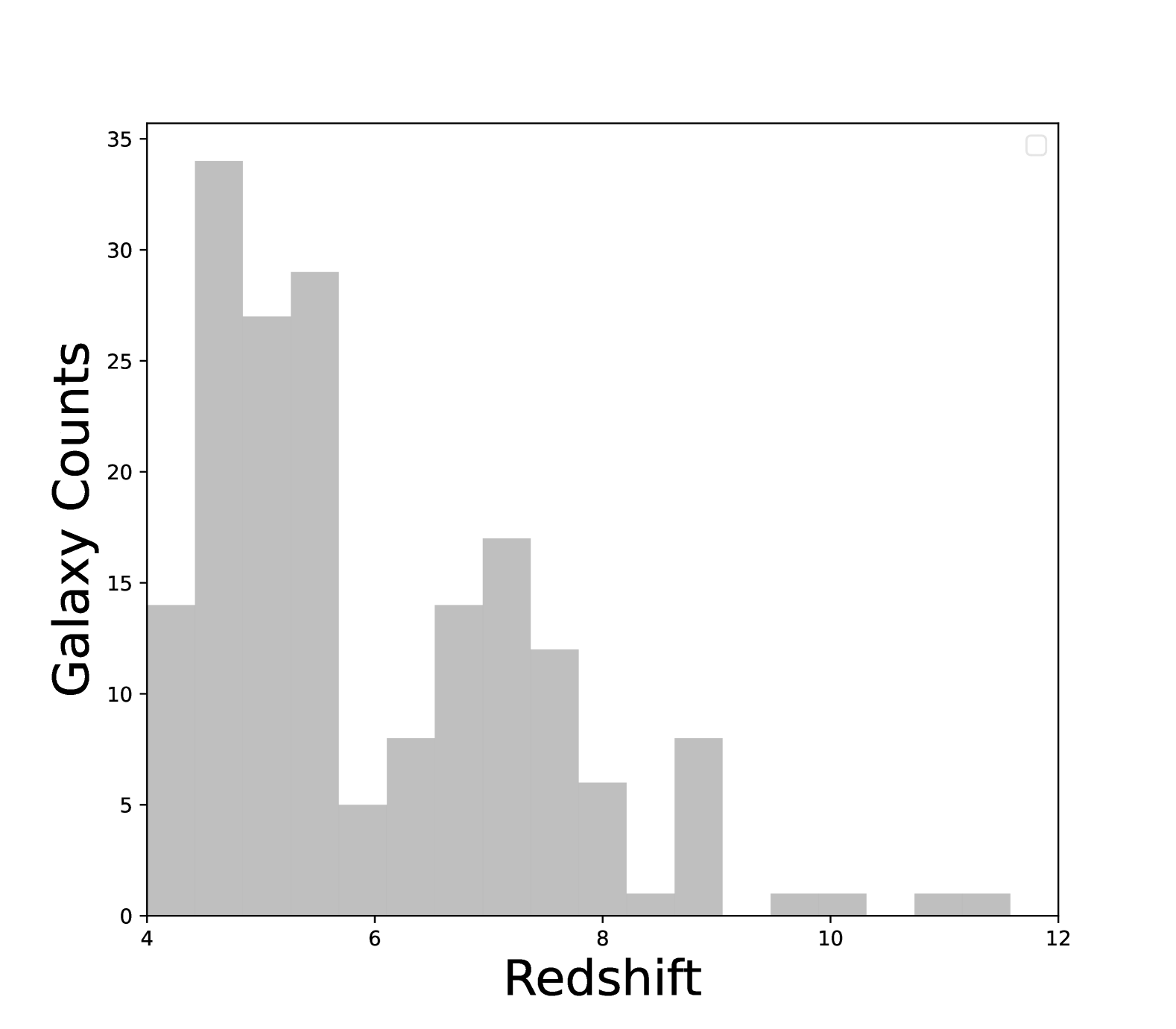
We have 1,337 spectroscopic observations with NIRSpec (Arrabal Haro et al. 2023) from CEERS. We use 634 of these NIRSpec observations carried out with the prism configuration. The spectroscopic targets were selected on the basis of CANDELS HST imaging (Grogin et al. 2011; Koekemoer et al. 2011) on various non-homogeneous criteria, which might introduce a bias in the selection. CEERS’s NIRCam observations detected 101,808 objects photometrically (CEERS_v0.51.4, Bagley et al. 2023). Whenever possible, we combine spectroscopic data (Birkmann et al. 2022) with photometric data by cross-matching the coordinates within 0.2 arcsec. However, because there is no complete overlap between CEERS NIRSpec and NIRCam observations, some NIRSpec fields are in areas where we have no NIRCam imaging. For them, we only use the spectroscopic data. After fitting the prism spectra (with and without NIRCam data), we check the quality of the spectroscopic redshifts for objects with z_spec $>$ 4.0. We classify the redshifts in four classes of redshift quality from q_z=0 (no doubts on redshift), to q_z=4 (wrong or unconfirmed redshift). We keep 173 objects with NIRSpec observations, for which q_z=0 (all modeled lines match the observed spectrum) or q_z=1 (some fainter lines not in excellent agreement with the models). Objects with q_z=2 present a continuum that could be in agreement with the derived redshift, but without any positively identified lines, and objects with q_z=3 only have a low signal-to-noise hint for the estimated redshift. We have flagged a sample of 6 possible AGN based on the literature (Kocevski et al. 2023; Larson et al. 2023; Harikane et al. 2023). These AGN are listed in Tab. 1, and shown with crosses in the plots. From this analysis, the distribution of redshifts is shown in Fig. 1. Most galaxies are clustered in the range z=4.0 to z=8.0, with a minority but important tail extending to z $\lesssim$12.

Table 1: This table extracted from Harikane et al. (2023) lists the possible AGNs in the analyzed sample. We keep them in the analysis but they are flagged in the figures.

id CEERS	redshift	RA	Dec
nirspec4_397	6.01	14:19:20.69	+52:52:57.7
nirspec8_717	6.94	14:20:19.54	+52:58:19.9
nirspec4_746	5.63	14:19:14.19	+52:52:06.5
nirspec8_1236	4.50	14:20:34.87	+52:58:02.2
nirspec7_1244	4.48	14:20:57.76	+53:02:09.8
nirspec4_2782	5.26	14:19:17.63	+52:49:49.0

Figure 1: Distribution of spectroscopic redshifts derived by fitting the spectrophotometric data with CIGALE. We keep 173 objects with the most robust redshifts. Galaxies are mainly found in two subpopulations at 4 $\lesssim$ z $\lesssim$ 6 and 5$\lesssim$ z $\lesssim$ 6, with a tail extending to z $\lesssim$ 12.

2.1.2 Analysis of spectrophotometric data

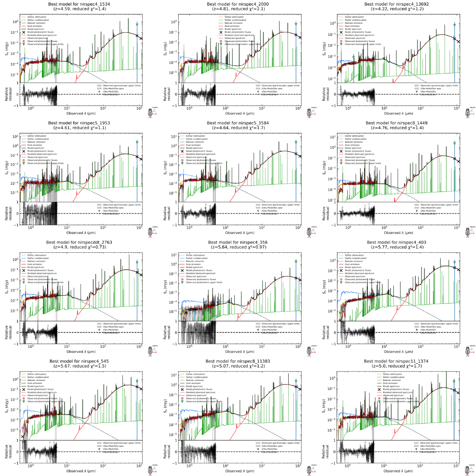
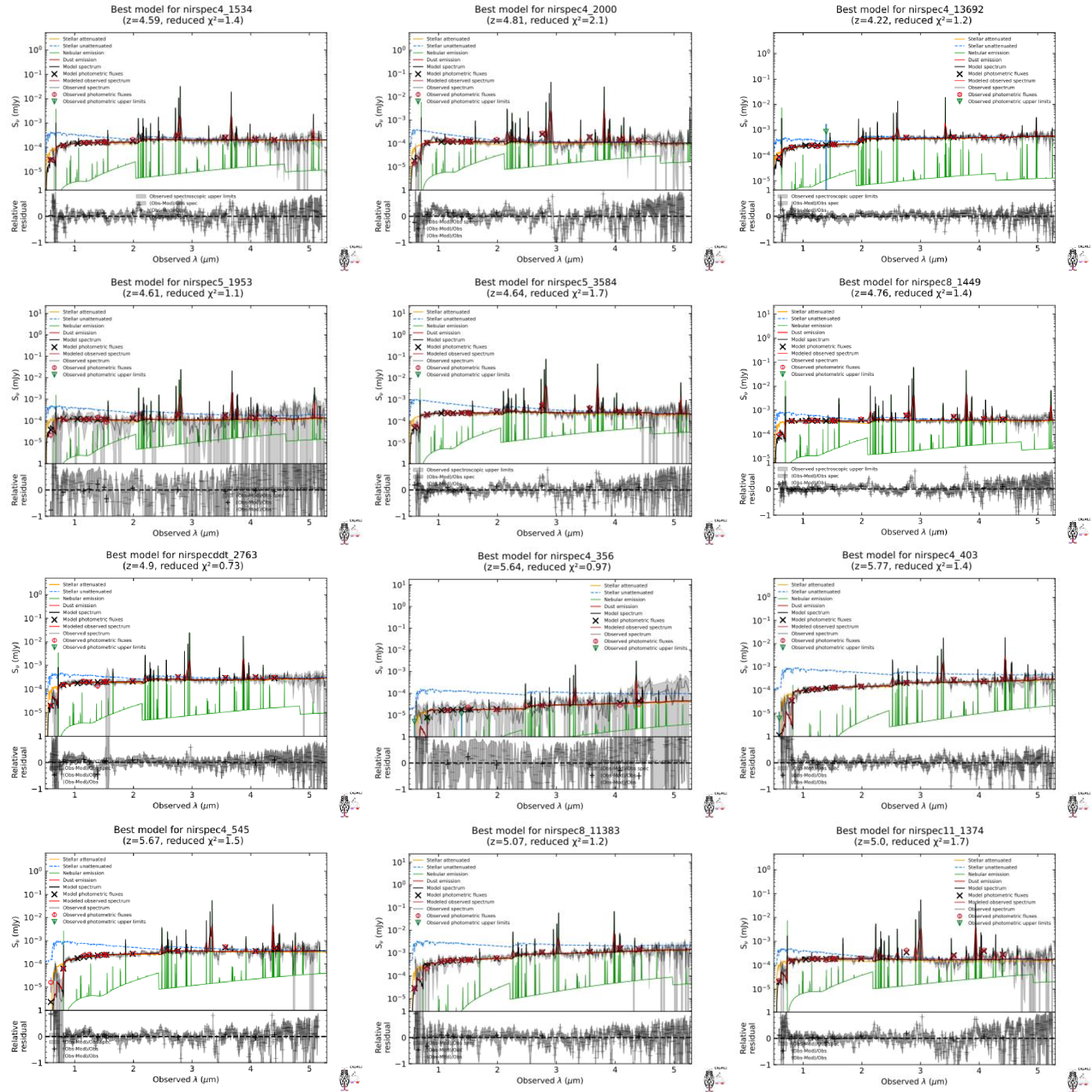
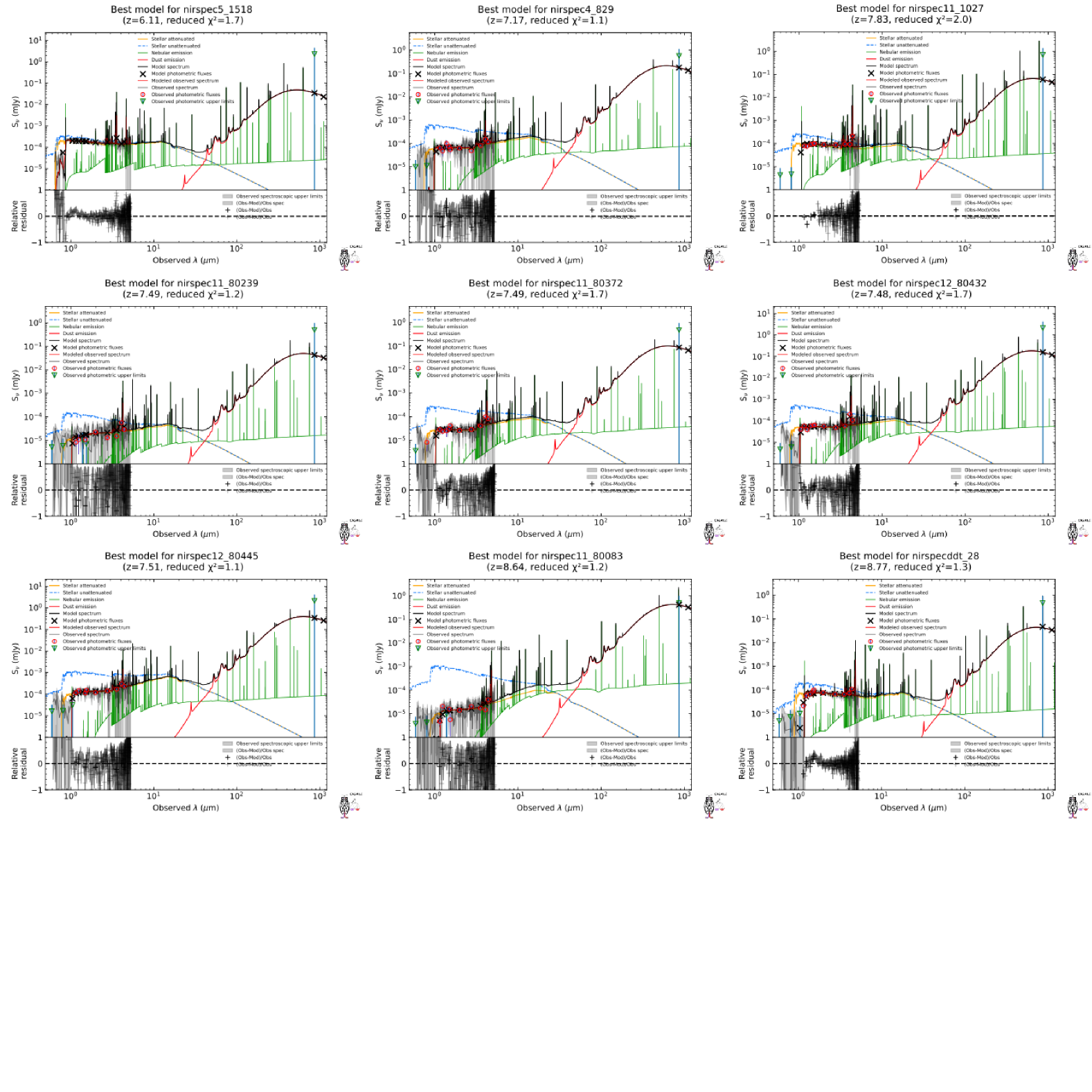
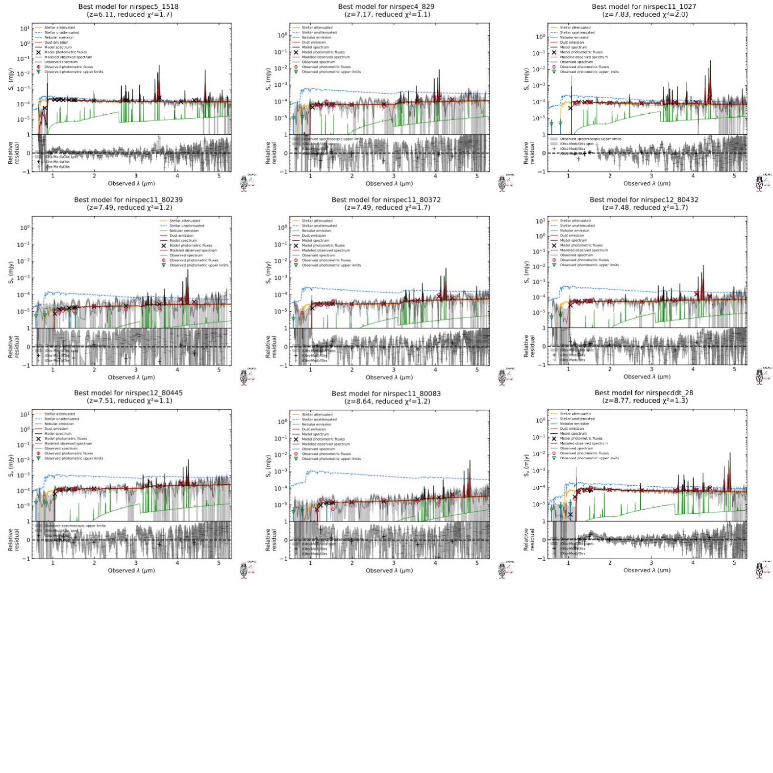
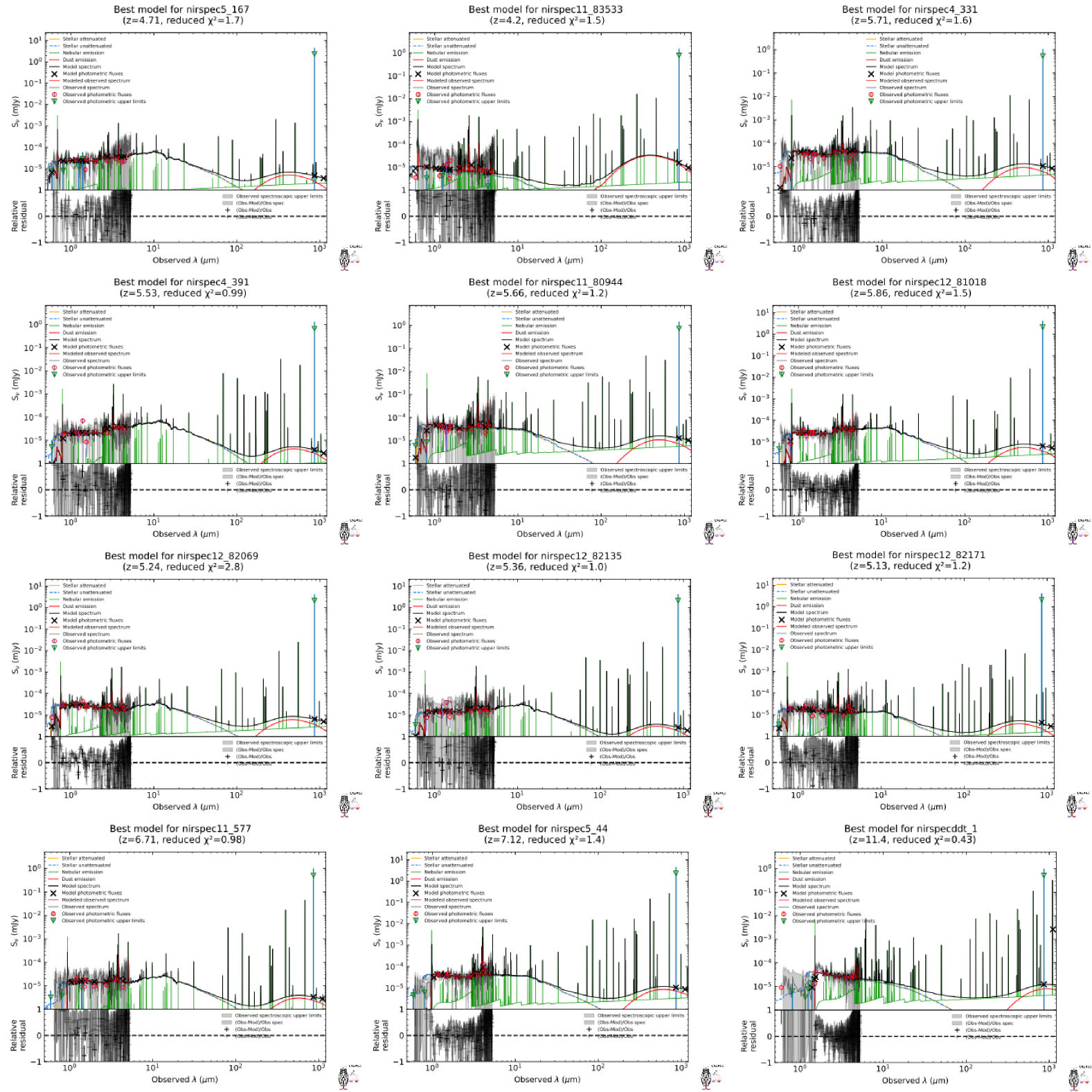
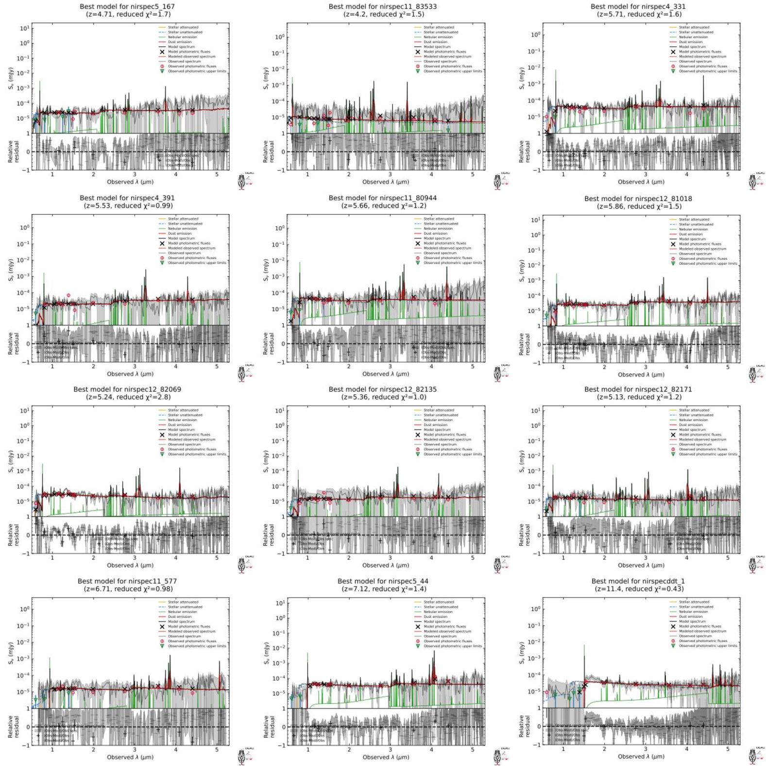
We use all data with a signal-to-noise ratio (SNR) SNR$>$1.0 per pixel in the spectrum and for each NIRCam photometric band. All other measures are set as upper limits in the fit. We utilize a new version of CIGALE that accepts both photometric and spectroscopic data (see the Appendix A) and we define this type of mixed data as spectrophotometric energy distributions (SPEDs) to clarify the difference from traditional spectral energy distributions (SEDs). The priors used in the fits are listed in Tab. 3 of the appendix B and a sample of the fits is shown in Figs. 20 to 25.

Two SFHs are used to test the stability of the results: a delayed-plus-burst and a periodic one. The delayed SFH assumes that star formation is active over a few tens to hundreds of Myrs with SFR(t) $\propto$ $\frac{t}{\tau^{2}}\times\exp^{-t/\tau}$ followed by a final burst with various possible ages. Various other types of SFHs could be used, but determining the SFH in the early universe is difficult for any SED modeling method (Lower et al. 2020). Moreover, Leja et al. 2019; Iyer et al. 2019; Tacchella et al. 2023 insist on the fact that the priors chosen for the fit are the primary drivers, before the type of SFH, to recover the physical parameters. The number of priors thus sets strong constraints on the ability to successfully run fitting codes, especially for large samples. The speed of CIGALE (Burgarella et al. 2024) allows it to explore various sets of priors with several 10⁸ models in a reasonable time for thousands of spectrophotometric objects. For the alternate SFH, a periodic SFH is chosen because it is conceptually different from the delayed-plus-burst SFH: it does not assume any kind of continuous SFH. Instead, a series of bursts, separated by regular quiescent periods, are used (see the appendix C that shows that this periodic SFH has a low impact on the results presented in this paper).

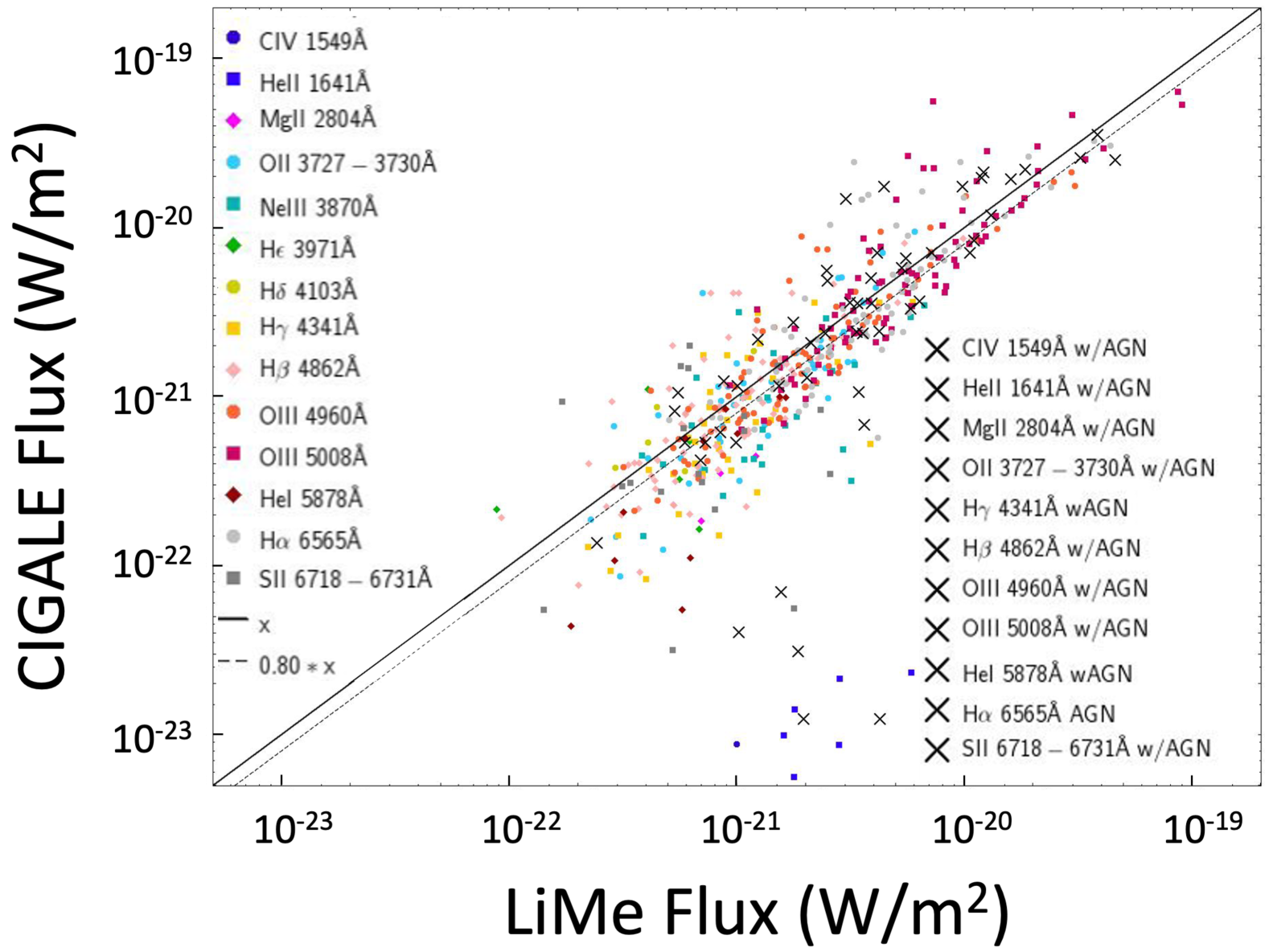
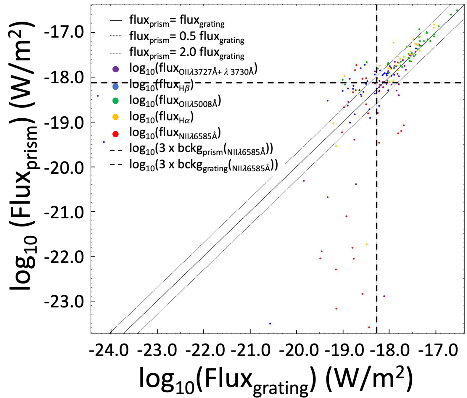
CIGALE estimates line fluxes through a comparison with Cloudy-derived nebular models included in CIGALE. To be sure we are on a safe ground, we validate the line fluxes measured by CIGALE with those estimated via other methods: we check in Figs. 2 and 3 that the flux of the emission lines measured by CIGALE are consistent with first fluxes estimated with the LiMe software (Fernández et al. 2024) and second, a fit performed on the sub-sample where both prism and grating NIRSpec spectra are available. For this second measurement, we fit the lines with lmfit (based on the Levenberg-Marquardt method). lmfit provides us with tools to perform non-linear optimization and curve fitting in Python. Practically speaking, we fit the lines per group of 3 lines (e.g. H$\beta$+[OIII] or [NII]+H$\alpha$) assuming a model which is the sum of 3 Gaussian distributions for the emission lines, plus a line to fit the continuum. The comparison is good up to line fluxes of about 3$\sigma$ of the local background.

Figure 2: Comparison of the CIGALE fluxes to those measured with LiMe (Fernández et al. 2024). The full results on the CEERS catalog redshifts and line measurements will be discussed in Arrabal Haro et al. (in preparation). The points corresponding to each emission line are color-coded to better identify each species (see inside caption). AGN lines are identified by crosses. The most ultraviolet lines (CIV $\lambda$1549 $\AA$, HeII $\lambda$1641 $\AA$ in the lower part of the plot, are not in agreement with those estimated by LiMe as shown by the offset from the solid 1-to-1 line. Instead, we find that other lines are systematically different by about about 20 % (dashed line). The observed difference might find an origin in the subtraction of the continuum.

Figure 3: Comparison of the fluxes computed by CIGALE (Flux_prism) with Gaussian fitting of the lines observed in the grating configuration (Flux_grating), for objects observed in both configurations. The points corresponding to each emission line are color-coded to better identify each species (see inside caption). The diagonal line shows the one-to-one relation (Flux_prism = Flux_grating) while the dashed lines present offsets (Flux_prism = 0.5 Flux_grating and (flux_prism = 2.0 Flux_grating). The horizontal and vertical dashed lines show the level of the 3$\sigma$ background around the [NII]+H$\alpha$ lines.

3 The properties of the galaxy sample

In this section, we define how we selected a specific population of 49 galaxies that have extremely low dust attenuation (GELDAs). We observationally define GELDAs using the following criteria:

• The FUV dust attenuation A_FUV = 0.0 within 2$\sigma_{A\_FUV}$,

• The stellar mass M_star $<$ 10⁹M_⊙

3.1 Star formation rate and stellar mass

Fig. 4 presents the histogram of the stellar masses derived by CIGALE for the present sample of galaxies. The structure of the histogram as a function of the UV slope $\beta_{FUV}$ confirms the relation between stellar mass and dust attenuation at high and ultra-high redshifts as shown by several papers (Bogdanoska & Burgarella 2020; Weibel et al. 2024; Bouwens et al. 2016).

Figure 4: Distribution of stellar masses derived by fitting the spectrophotometric energy distributions of our galaxy sample. In this plot, we only show galaxies with $\beta_{FUV}$ derived from CIGALE’s fits. The range of stellar masses reaches M_star values as low as a few 10⁷ M_⊙. The color coding shows that the least massive galaxies clearly have bluer UV slopes: $\beta_{FUV}\leq-2.2$ while the most massive galaxies have redder slopes: $-1.5<\beta_{FUV}$, as expected from the dependence of UV dust attenuation on stellar mass (see, e.g. Bogdanoska & Burgarella 2020; Weibel et al. 2024; Bouwens et al. 2016). The vertical numbers show the mean stellar mass for each sample.

Figure 5: This plot presents the star formation rate as a function of the stellar mass for our galaxy sample. For some galaxies the observed spectra are not good enough to provide a trustworthy fit of the spectrum (f${}_{\lambda}\propto\lambda^{\beta}_{FUV}$) for the UV slope. For those galaxies, we rely on CIGALE’s fits. Here, the larger symbols correspond to UV slopes spectroscopically estimated from the observed data while the smaller symbols are from the CIGALE fits. Blue, green and red symbols respectively show galaxies with blue, intermediate and red slopes (see inside caption). Whatever the origin of the UV slopes, the lower mass galaxies present a bluer UV slope while the more massive have are redder. We superimpose in this plot the best-fit main sequence from Speagle et al. (2014) in the range z = 4 to z = 12, color coded from magenta to dark red (bottom to top).

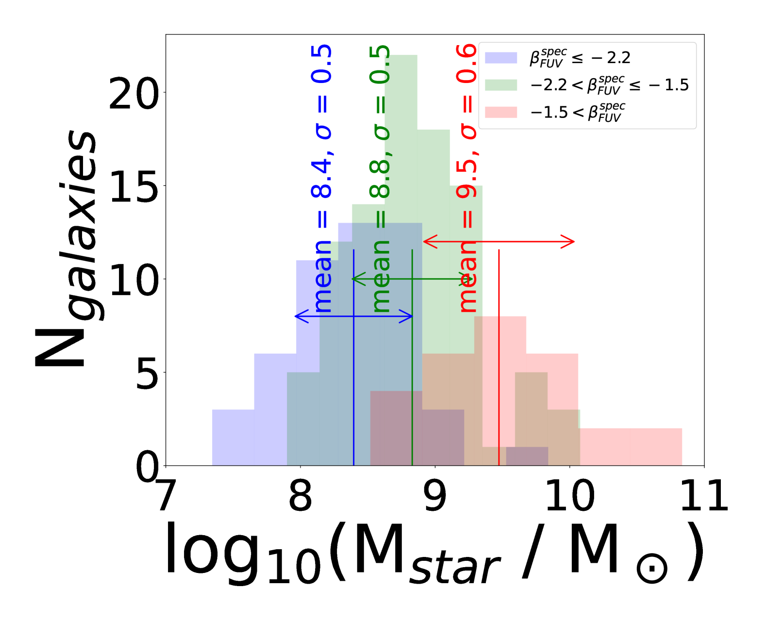
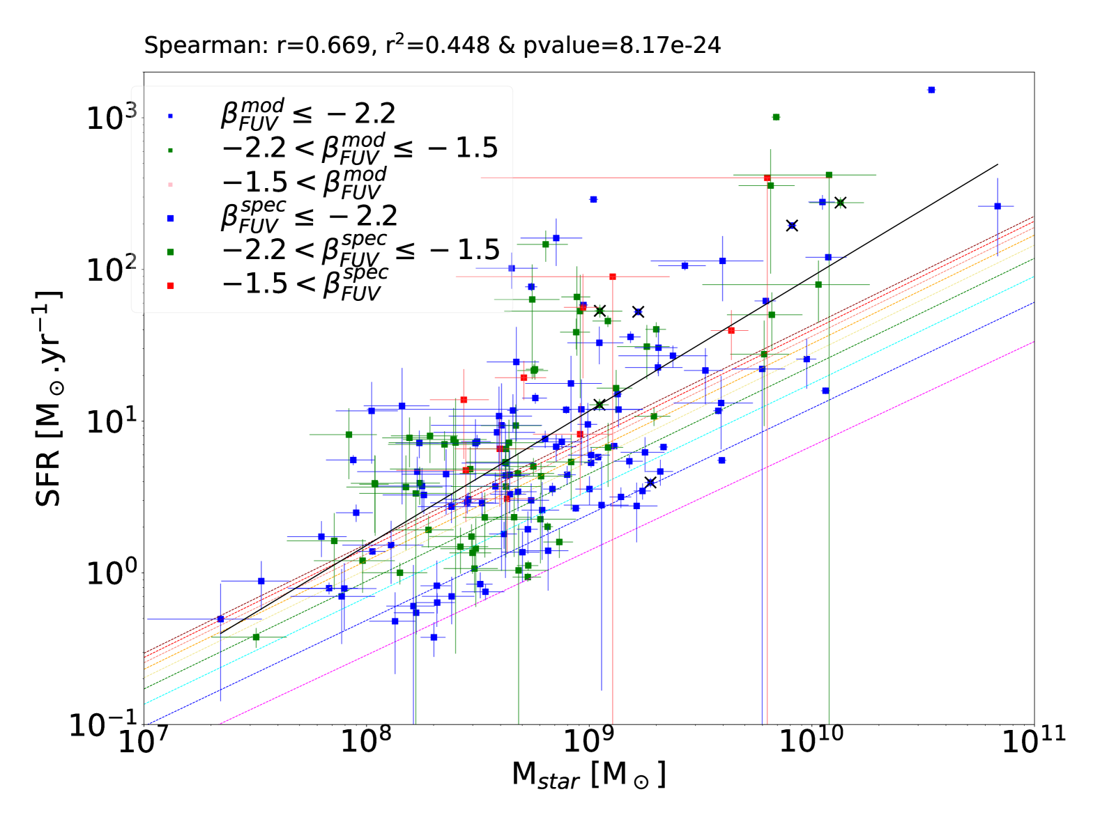
Fig. 5 shows the location of the MS in the SFR vs. M_star diagram. Because the redshift range is quite large, we might not expect all galaxies to follow a tight sequence. However, since most of the sample is in the redshift range 4$<$z$<$6 (Fig. 1), we do observe such a sequence, which is structured by the UV slope $\beta_{FUV}$. We do not see any noticeable differences between UV slopes derived by directly fitting the spectra and those derived by fitting the SPEDs with CIGALE. In Fig. 5, we present a comparison of the location of our sample with the best-fit main sequence from Speagle et al. (2014). The fits from Speagle et al. (2014) show the well-known strong increase in SFR at low redshifts (z$\lesssim$8) followed by a gradual lower increase at higher redshifts up to (z=12). Our sample of objects are mainly in the first redshift bin (4$\lesssim$z$\lesssim$8, see Fig. 1). They are MS galaxies. However, part of the sample lies above the highest MS from Speagle et al. (2014), especially the reddest. They likely belong to a star-busting class of galaxies. AGN are preferentially found at large masses and high SFRs.

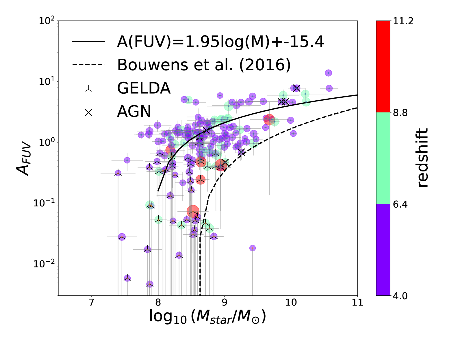
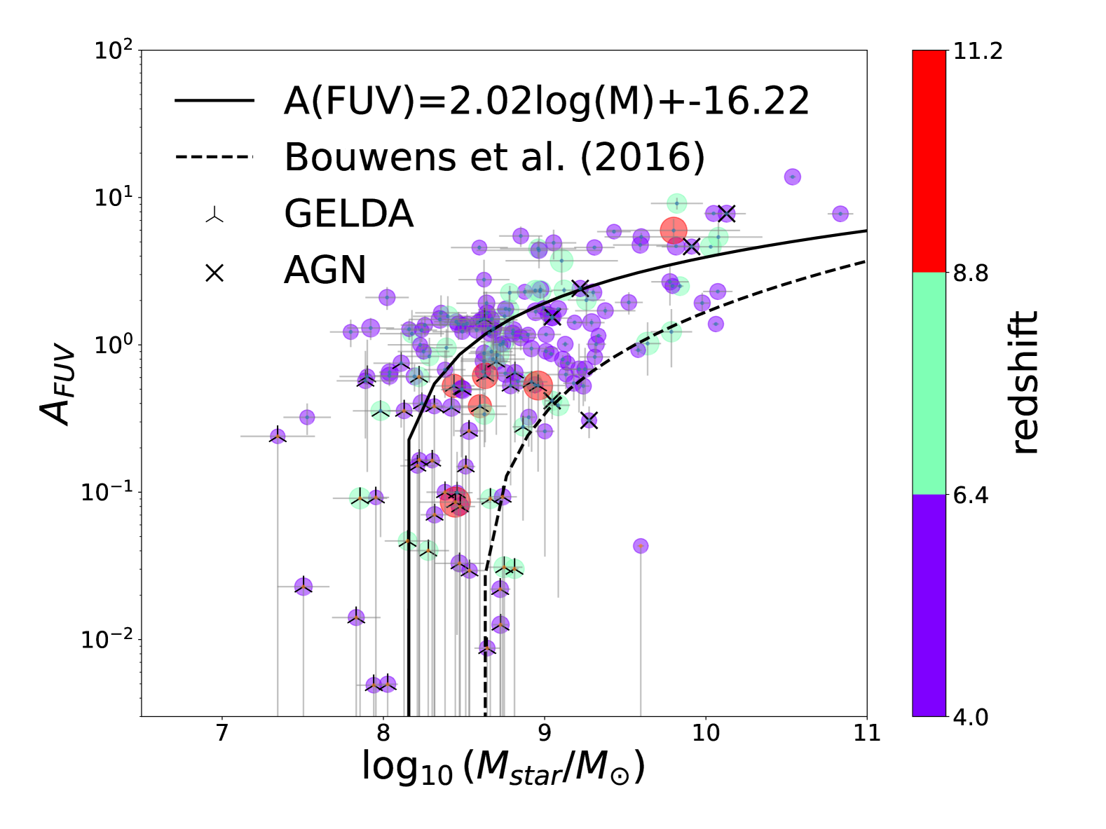
In Fig. 6, we show the far-UV dust attenuations, A_FUV, vs. $\log_{10}$(M_star) where we again note a large dispersion at low M_star spanning more than 2 decades. The stellar mass is not the only acting parameter as both low and relatively high A_FUV lie in the same stellar mass range. We do not observe any clustering of low-redshift galaxies (z $\lesssim$ 8.8) in the lower part of the plot. This shows that these low-redshift galaxies could have a wide range of dust attenuation. On the other hand, five out of six of the highest redshift galaxies (z $\gtrsim$ 8.8) are found in this part of Fig. 6, and are therefore GELDAs. This would suggest that GELDAs become dominant in the early Universe.

The ‘consensus’ law between A_FUV and M_star estimated at the lower redshift (z$\sim$2-3) by Bouwens et al. (2016) does not pass through the present data. Bogdanoska & Burgarella (2020) found that this ‘consensus’ law does not appear to be valid at large redshifts. They also suggested that the low stellar mass galaxies exhibit a large scatter in A_FUV and proposed an evolution of this A_FUV and M_star relation with the redshift. However, the sample available in Bogdanoska & Burgarella (2020) could hardly reach $\log_{10}$(M_star) $\lesssim$ 9.0. JWST sensitivity to much fainter flux allows one to reach galaxies at much lower stellar masses, and potentially also permits one to detect this new population of GELDAs.

Figure 6: Far-UV dust attenuation A_FUV as a function of the stellar mass, $\log_{10}$(M${}_{star})$. The symbols are color-coded and sized with the redshift. The red objects corresponds to the highest redshift bin defined in this paper (z $>$ 8.8). The majority of highest-redshift GELDAs (5 out of 6) are found in the low-A_FUV part of the plot. This sample of galaxies at z $>$ 8.8 is small, but it might confirm an expected decreasing evolution of the dust attenuation with the redshift. The dashed line is the ‘consensus’ law from Bouwens et al. (2016) while the continuous line is the best linear fit (A_FUV vs $\log_{10}$(M_star)) to the present data. GELDAs are shown with upside-down Y and AGN with crosses.

3.2 The mass of metals and gas of the galaxy sample

In CIGALE, the stellar Z_star and nebular Z_gas metallicities have different priors. This is most useful when spectroscopic data are available because they allow to separately constrained both metallicities by fitting the spectra, including lines. For this specific estimation process, CIGALE makes use of the new nebular models described in Theulé et al. (2024) that can have excitation parameters up to logU = -1.0 and with a wide range of nebular metallicities and electronic densities (n_H). The metallicity Z_gas derived by CIGALE can be converted into 12+$\log_{10}$(O/H) where O/H is the oxygen abundance of the gas by using their table 1 (correspondence between $\xi_{0}$, the interstellar gas metallicities and the stellar metallicities). $\xi_{0}$ is defined on oxygen abundance: $\xi_{0}$ = (O/H) / (O/H)_GC, where (O/H)_GC = 5.76 $\times$ 10^-4, and GC is the so-called local Galactic concordance (Theulé et al. (2024) follows Nicholls et al. 2017). From this, Eq. 1 links total metallicity to oxygen abundance:

$${\rm Eq.\leavevmode\nobreak\ 1:\leavevmode\nobreak\ }12+\log_{10}(O/H))=\log_{10}(Z_{gas})+10.410.$$

In Fig. 7, we compare the CIGALE metallicities estimated for the same CEERS galaxies by Nakajima et al. (2022, 2023) and Sanders et al. (2024). Nakajima et al. (2023) measured emission line fluxes for 135 galaxies (115 in CEERS). For 10 of these galaxies, they determined their electron temperatures with [O III] $\lambda$4363 $\AA$ lines, in a way similar to lower redshift star-forming galaxies, and they derived the metallicities by a direct method. They finally estimated metallicities for their entire sample of JWST-observed galaxies with strong lines using their previous metallicity calibration (Nakajima et al. 2022), based on the direct method measurements. Our sample common with Nakajima et al. (2023) amounts to 90 galaxies. Sanders et al. (2024) also combine JWST measurements with [O III] $\lambda$4363 $\AA$ auroral line detections from JWST/NIRSpec and from ground-based spectroscopy to derive electron temperature (T_e) and direct-method oxygen abundances on a combined sample of 12 star-forming galaxies at z=1.4-8.7. Our sample shares 3 of them, for which we derive metallicities with CIGALE. Finally, Nakajima et al. (2023) and Sanders et al. (2024) have 3 common objects. Our fitting method is different, as the total spectrophotometric fits allow one to consistently constrain the metallicities (Z_star and Z_gas) by selecting only models that agree with the whole information brought by observations, that is, continuum and lines, together.

The metallicities estimated by CIGALE show a systematic or gradually increasing discrepancy at $\log_{10}(O/H)<7.4-7.6$ with Nakajima et al. (2023) with metallicities lower by about $\sigma$ ($\log_{10}$(O/H))¡0.10. However, we note that the direct method is not well calibrated below $\log_{10}(O/H)<7.4-7.6$ with less auroral measurements for objects at these low metallicities. The true value becomes quite uncertain until we could get a better calibration. Fig. 8 shows that individually and globally the metallicity estimates can vary depending on the method used to derive metallicities from the lines. The CIGALE metallicities estimated by fitting the entire spectrum are found close to most values from Nakajima et al. (2023) and Sanders et al. (2024), and especially very close to the R23 index which is found to be the most reliable among various metallicity indicators over the wider range of metallicity (Nakajima et al. (2022)). However, the line ratios involving nitrogen lines (N2 and O3N2 from Nakajima et al. (2023) lead to much lower metallicities by about 1 dex. Nakajima et al. (2022) found a scatter as large as $\Delta\log_{10}$(O/H) $\sim$ 0.4 dex in the relation for metallicities derived using the N2 index. This is especially true at low metallicities, as for our galaxies. They suggested that this might be associated with line ratios that use single-ionized, low-ionization lines such as [NII]. We conclude that care should be taken when using only one of these indices. However, CIGALE provides us with a safe and reliable method for estimating metallicities, at least in the present range.

Figure 7: Difference between metallicity estimates (12+$\log_{10}(O/H)$ defined in Eq. 1): a comparison of the metallicities measured for some of our galaxies in the literature (Nakajima et al. 2022, 2023; Sanders et al. 2024) via auroral lines, with our own estimates. At relatively high metallicities, above 12+log10(O/H)$\sim$7.4-7.6 (that is Z/Z_gas 0.1-11% Z_⊙), the differences remain within $\sigma$(12+$\log_{10}(OH))$$<$0.05. This is about the same dispersion between other metallicity estimates, although on a smaller sample. However, there is a disagreement at lower metallicities, and CIGALE’s 12+$\log_{10}$(O/H) present an offset that might be systematic or increasing with lower metallicities by about $\sigma$ ($\log_{10}$(O/H))$<$0.10. But the direct method is not well calibrated at $\log_{10}$(O/H)$<$7.4-7.6 because there are less than 5 objects with auroral lines at such low metallicities estimated via the direct-method oxygen abundances.

Figure 8: Direct comparison of metallicities (12+$\log_{10}(O/H)$ defined in Eq. 1. Left: this panel shows the metallicities derived using various published calibrations as a function of the mean metallicities computed from each measured galaxy. The dashed black line is the 1-to-1 relation. For a given metallicity on an x-axis, we could get a very wide range on the y-axis depending on which line ratio is used. The black dots are the metallicities from CIGALE. The red-orange ones from Nakajima et al. (2023) and the blue-green one from Sanders et al. (2024). The color coding is given in the legend inside the plot. Right: this panel presents the same information with a rolling average. Most of the metallicity values agree within about $\pm$ 0.5 dex and the metallicities from CIGALE are approximately in the middle range. However, we notice that the ones involving the nitrogen lines lead to much lower metallicities (see text for more details.

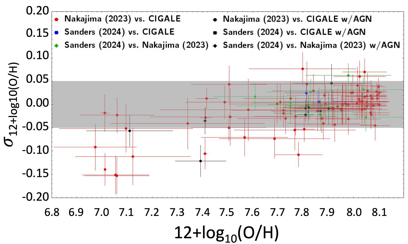
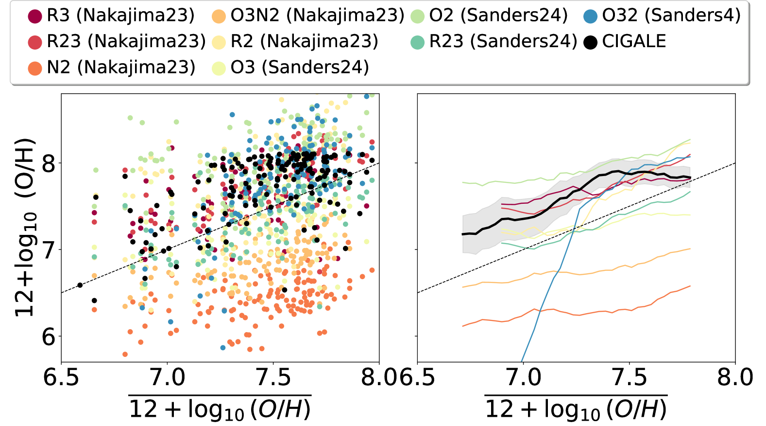
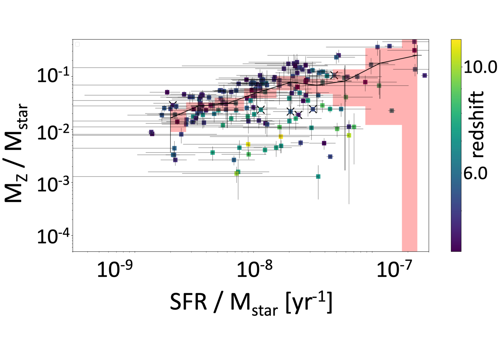
Fig. 9 presents the specific mass of metals (M_Z/M_star) for the present sample as a function of the specific SFR (SFR/M_star), where the metal mass, M_Z is computed from Eq. 2 (Heintz et al. 2023b):

$${\rm Eq.\leavevmode\nobreak\ 2:\leavevmode\nobreak\ }M_{Z}=M_{gas}\times 10^{12+log_{10}(O/H)-8.69}\times Z_{\odot}$$

In Eq. 2, the gas mass, M_gas, and the oxygen abundance, 12+$\log_{10}$(O/H), are estimated via the spectrophotometric fitting and from Eq. 1. To estimate M_gas, we need to estimate the molecular mass M_molgas from Eq. 3 (Tacconi et al. 2020).

$${\rm Eq.\leavevmode\nobreak\ 3:\leavevmode\nobreak\ }log_{10}(M_{molgas})=$$

$$0.06-3.33\times[log_{10}(1+z)-0.65]^{2}+$$

$$0.51\times log_{10}(sSFR/sSFR(MS,z,M_{star})$$

$$-0.41\times[log_{10}(M_{star})-10.7]\times M_{star}$$

where the specific instantaneous SFR, sSFR=SFR_inst/M_star, is derived from the spectrophotometric fitting, while the reference sSFR for the MS as a function of the stellar mass M_star, and the redshift: sSFR(MS, z, M_star) is from Speagle et al. (2014), assuming the so-called ”Bluer” w/ high-z obs” MS in their Table 9 (Eq. 4). The MS is modeled up to z$\sim$6, while our sample reaches z=11.4. However, even if the scatter in the MS is quite large, studies suggest that it should not show any strong evolution to z$\sim$12 (Cole et al. 2025; Chakraborty et al. 2024).

$${\rm Eq.\leavevmode\nobreak\ 4:\leavevmode\nobreak\ }\log_{10}(SFR(M_{star},Age_{Universe}))=$$

$$[(0.73-0.027\times Age_{Universe})\times\log_{10}(M_{star})-$$

$$(5.42+0.42\times Age_{Universe})]-\log_{10}(M_{star})$$

We also need to add the contribution from the atomic gas M_atomgas to M_molgas The atomic-to-molecular mass ratio M_atomgas/M_molgas is estimated by Chowdhury et al. (2022) for star-forming galaxies at z$\sim$0, z$\sim$1.0, and z$\sim$1.3 with values in the range 4$\pm$2 for galaxies with M_star$>$10¹⁰ M_⊙. To account for galaxies with $<$10¹⁰ M_⊙ in their statistics, they assume that the ratios M_atomgas to M_molgas are systematically higher by a factor of about 5 for all galaxies with M_star $<$ M_⊙. In this case, the values obtained would increase M_molgas at z $\sim$ 1.3 by a factor of approximately 2, giving a ratio M_atomgas/M_molgas = 2.5 for the highest redshifts. At higher redshifts (0.01 $<$ z $<$ 6.4), there is no significant redshift evolution of the M_atomgas/M_molgas ratio (Messias et al. 2024), which is about 1-3. At z=8.496, the gas and stellar contents of a metal-poor galaxy are studied with JWST and ALMA (Heintz et al. 2023a). From this analysis, they infer M_molgas = (3.0-5.0) $\times$ 10⁸ M_⊙. corresponding to 40% $\pm$ 10% of M_gas for their object, which leads to M_atomgas/M_molgas = 1.5${}^{2.0}_{1.3}$. Given the redshift of our objects, we will assume in this paper M_atomgas/M_molgas=2.0${}^{2.5}_{1.3}$.

Figure 9: We present the evolution of the metal-to-stellar mass ratio as a function of the specific star formation rate in this metal formation rate diagram (MFRD) in the same way we defined the dust formation rate diagram (DFRD) that shows how the specific dust mass (M_dust/M_star) changes with the specific star formation rate (SFR/M_star) in Burgarella et al. (2022). This type of diagram is normalized to M_star and allows a better comparison between galaxies. The symbols are color-coded with the redshift. The pink-shaded area presents the 2-$\sigma$ confidence interval for the distribution in $M_{Z}$/M_star, and the black solid line shows the rolling average. We observe a decreasing trend with decreasing sSFR. The highest-redshift galaxies are located in the lowest part of the plot.

3.3 Dust masses

Dust masses (M_dust) are very important for building diagnostics on the origin of dust in galaxies because they are directly related to the dust building rate, which in turn can provide us with information on the origin of dust grains (e.g., Leśniewska & Michałowski 2019; Nanni et al. 2020; Burgarella et al. 2022). To help estimate the dust masses for our objects, we use deep 450 and 850 $\mu$m SCUBA-2 and NOEMA-1.1 mm observations. Both are cross-correlated with JWST’s coordinates. The former have a mean depth of $\sigma_{450}$=1.9 and $\sigma_{480}$=0.46 mJy beam^-1 and the angular resolution is $\theta_{FWHM}$ $\approx$ 8 arcsec at 450 $\mu$m, and $\theta_{FWHM}$ $\approx$ 14.5 arcsec at 850 $\mu$m. For NOEMA, the rms is $\sigma_{1.1mm}$=0.10 mJy beam^-1, and the beam size is 1.35 $\times$ 0.85 arcsec². Although the sensitivity of these observations is typically lower than that required to detect most of our galaxies, the inferred upper limits are useful to put constraints on the total IR luminosities and dust masses. Similarly, the angular resolutions are much larger than JWST’s (Zavala et al. 2023). Some of the associations might therefore be wrong. However, these sub-mm data rule out any strong lower-redshift far-IR emitters that would be associated with the objects in our sample.

The far-IR information for this sample is limited and we cannot directly derive any information on the dust emission SED shape. However, the ALMA-ALPINE sample e.g. Béthermin et al. 2020; Pozzi et al. 2021; Sommovigo et al. 2022a and the ALMA-REBELS samples (e.g. Inami et al. 2022; Sommovigo et al. 2022b; Algera et al. 2024b and Algera et al. 2024a presents physical properties, e.g. stellar masses: $\log_{10}$(M_star)$\sim$10, redshifts: 4.5$<$z$<$6.2 similar to ours (Burgarella et al. 2022; Nanni et al. 2020). Due to the similarities of the samples, we will assume that we can make use of the same Draine et al. (2014) best-fit model (see Tab 3) identified in Burgarella et al. (2022); Nanni et al. (2020). We note that this ALMA-ALPINE model corresponds to a dust temperature T_dust=54.1$\pm$6.7 K, assuming an optically thin modified black-body, which is in good agreement with Sommovigo et al. (2022a) who found an average value $<T_{dust}>$=48 $\pm$ 8 K and M_dust in the range (0.5-25.1)$\times$ 10⁷ M_⊙ for ALPINE. For ALMA-REBELS, the median T_dust is in the 39-58 K range, and the median dust masses are estimated in the range (0.9-3.6)$\times$ 10⁷ M_⊙ (Sommovigo et al. 2022b). Sommovigo et al. (2022b) also predict that dust masses can be produced by SNae alone for 85 % of the REBELS sample. We note that Algera et al. (2024b, a) found lower dust temperatures (T_dust=30 - 35 K) for two objects in the REBELS sample. Furthermore, Sommovigo et al. (2022a) predict that more metal-poor high-z galaxies could have warmer temperatures because of their smaller dust content, while the objectives studied in Algera et al. (2024b, a) are metal-rich. However, the dust model is assumed to be the same in our work for all of our objects. Globally modifying our model would cause an offset of all the dust masses, but not the observed relative difference between GELDAs and non-GELDAs.

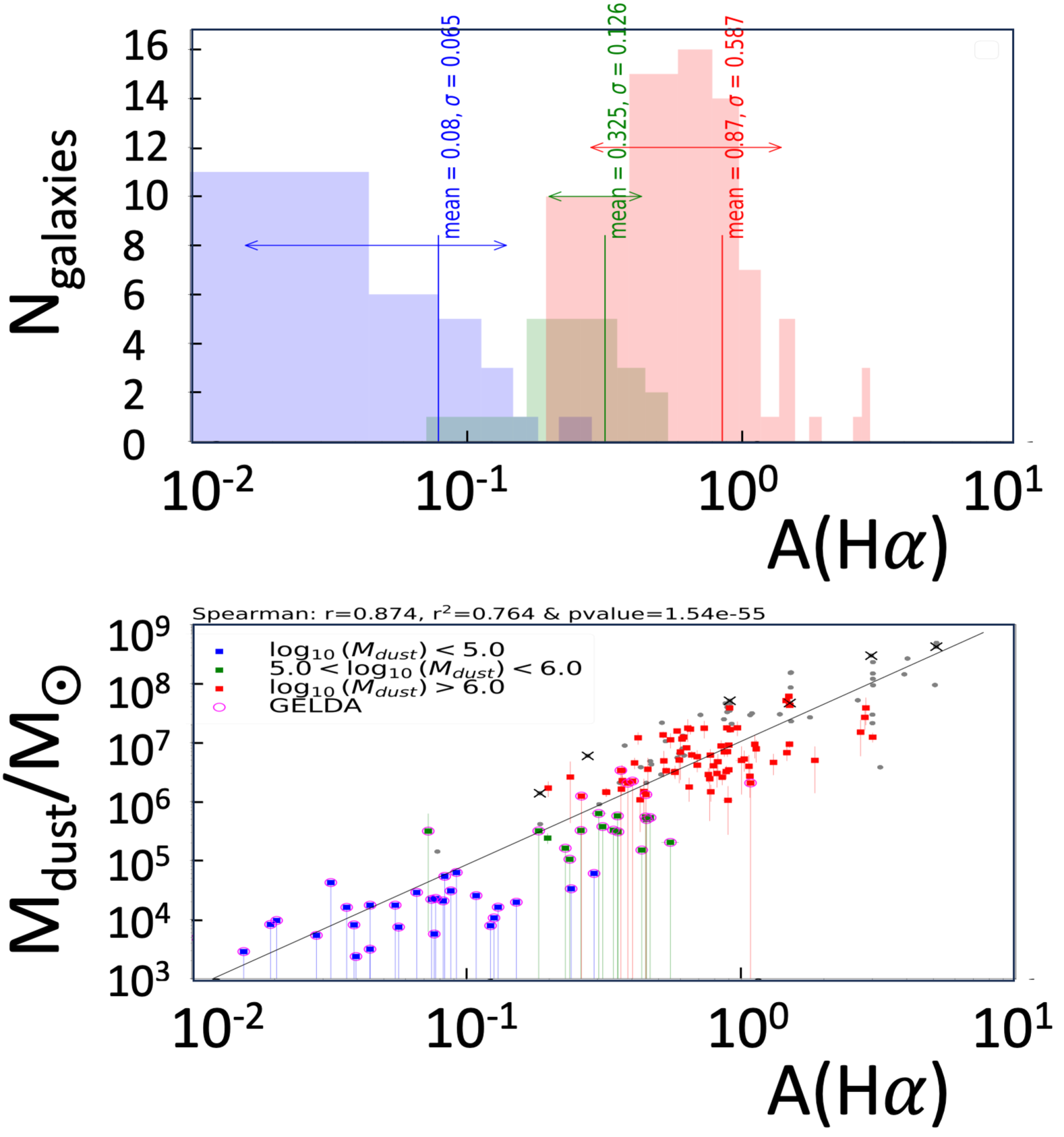
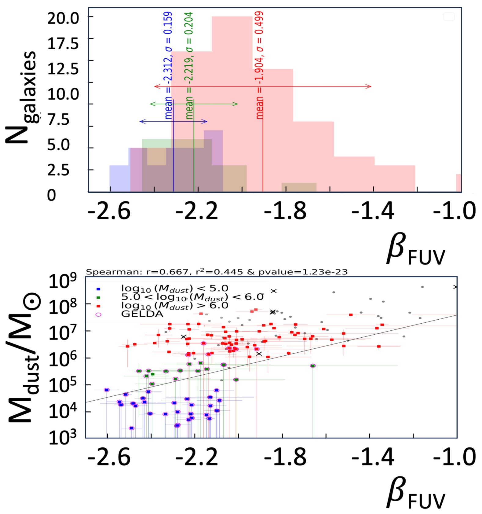
Because we use the above single dust emission model (Draine et al. 2014), we do not derive any shape for the IR emission in this paper. The shape of the IR spectrum is fixed by the ALMA-ALPINE sample at 4.5$<$z$<$6.2, and the IR luminosity is estimated assuming the energy balance concept; M_dust is constrained by the amount of dust attenuation and by the main observables that define this dust attenuation. Information on the amount of dust attenuation comes from the line ratios, especially H$\alpha$/H$\beta$ when available, the UV slope $\beta_{FUV}$, and from any available IR/sub-mm data (Figs. 10 and 11).

The analysis of the results suggests that the SCUBA-2 sub-mm fluxes do not significantly help in constraining the dust mass (see Fig.28), as we do not find any correlation between the measured fluxes or upper limits. NOEMA detections are deeper and provide flux densities that are more useful in constraining the dust mass. However, we only have two objects in the sample and none of them within the lower sequence of GELDAs. The Balmer decrement H$\alpha$/H$\beta$ and the dust attenuation for H$\alpha$, A(H$\alpha$) are strongly correlated with M_dust (see Fig. 10) correlation coefficient r_Hα/Hβ=0.874). The UV slope $\beta_{FUV}$ is also (see Fig. 11), although at a lower level, correlated with M_dust.(correlation coefficient r_{β_FUV}=0.667). We can thus conclude that, first, the emission lines, and second, the continuum shape drive the estimation of the amount of energy transferred into the far-IR. For our galaxy sample, the observed NIRSpec spectrum from about 0.5 to 5.3 $\mu$m provides the best spectral information to estimate the amount of dust attenuation via the Balmer decrement and the UV slope. Then, using the energy balance hypothesis, we can estimate the IR luminosity and thus M_dust, if the IR spectrum from Burgarella et al. (2022) is assumed to be valid for our present sample.

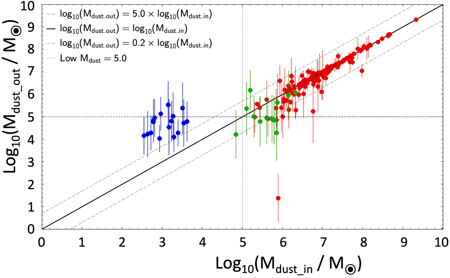
We perform tests that suggest that the minimum dust mass that we could estimate with CIGALE with the above assumptions is $\log_{10}$M_dust = 5.0 (Fig. 12). To perform these tests, we use the ability of CIGALE to create a mock catalog based on the best-fit SPEDs for each object derived from a first fit. To these best-fit SPEDs, we add the observed noise drawn assuming a Gaussian distribution (see Boquien et al. 2019 for a more detailed explanation).

Figure 10: Correlation of the estimated dust mass, M_dust with the dust attenuation, A(H$\alpha$). The most relevant parameter to predict the dust mass is the dust attenuation A(H$\alpha$) derived from the H$\alpha$/H$\beta$ Balmer decrement. The correlation with A(H$\alpha$) alone accounts for 76% of the variation in M_dust. The spectral information brought by NIRSpec is thus fundamental to estimate the dust masses. Blue, green and red symbols respectively mean M_dust $\leq$ 10⁵ M_⊙, 10⁵ $<$ M_dust $\leq$ 10⁶ M_⊙ and M_dust $>$ 10⁶, while magenta circles show GELDAs.

Figure 11: Same colors as in Fig. 10. Correlation of the estimated dust mass, M_dust with the UV slope $\beta_{FUV}$. The correlation with $\beta_{FUV}$ alone accounts for 44 % of this variation, which confirms that the spectral information on lines is the most important one. The other tested parameters: metallicity (about 2 %) and redshift ($<$ 1%), but also the level of the sub-mm upper limits are not significantly correlated with M_dust in this analysis.

In Fig. 13 we compare the trends related to the increase in the specific mass of metals (M_Z/M_star) and of dust (M_dust/M_star) with cosmic ages and with the star formation rate sSFR=SFR/Mstar. Several points can be noticed: first, both follow a similar trend; second, M_Z/M_star is always higher than M_dust/M_star: the mass of metals is larger than the dust mass; Third, we observe a lack of extremely low-metallicity galaxies: all the galaxies observed so far are above a critical metallicity value (Bayesian values derived by CIGALE) of about Z_crit=10^-3.

Figure 12: Use of a mock analysis to estimate the minimum dust mass that we can actually estimate using our approach. Top: The x-axis shows the modeled M_dust computed from the best-fit models and for each of our galaxies. CIGALE is able to recover (y-axis) by fitting the mock data, these input dust masses, down to about $\log_{10}$(M_dust) = 5.0. Parts of the objects in green and all the objects in blue should thus be considered as upper limits. These objects that are the ones identified as transitioners between the upper sequence and a possible lower sequence, are well below the prime sequence (red dots). Bottom: in this $\log_{10}$(M${}_{dust})$ vs. $\log_{10}$(M${}_{star})$ diagram, we can see that the lowest dust masses correspond to the lowest stellar masses. However, for the same stellar mass range, we do observe a wide range of dust masses. Normal, mid and low M_dust respectively mean M_dust $\leq$ 10⁵ M_⊙, 10⁵ $<$ M_dust $\leq$ 10⁶ M_⊙ and M_dust $>$ 10⁶ M_⊙.

Figure 13: The evolution of the mass of metals and mass of dust: M_Z/M_star (blue dots) and M_dust/M_star (red dots) both regularly increase with the age of the Universe (top): more metals and dust grains are formed as the Universe ages. We note that even for galaxies (blue symbols) in the early Universe (age_Universe $\lesssim$ 600 Myr or z$\gtrsim$9), M_Z/M_star never goes below a few 10^-3, possibly suggesting a fast rise of metals that produces the observed threshold. M_Z/M_star increases faster than M_dust/M_star, with a much larger dispersion for M_dust/M_star. The light blue/red area show the mean and 2$\sigma$ confidence interval of the distribution within several bins. b) M_Z/M_star (in blue) and M_dust/M_star (in red) decrease from high to low sSFR (bottom) as also shown in e.g. Palla et al. 2024; Shivaei et al. 2022. We also note here a larger dispersion at lower sSFR for M_dust/M_star, but only for M_dust/M_star.

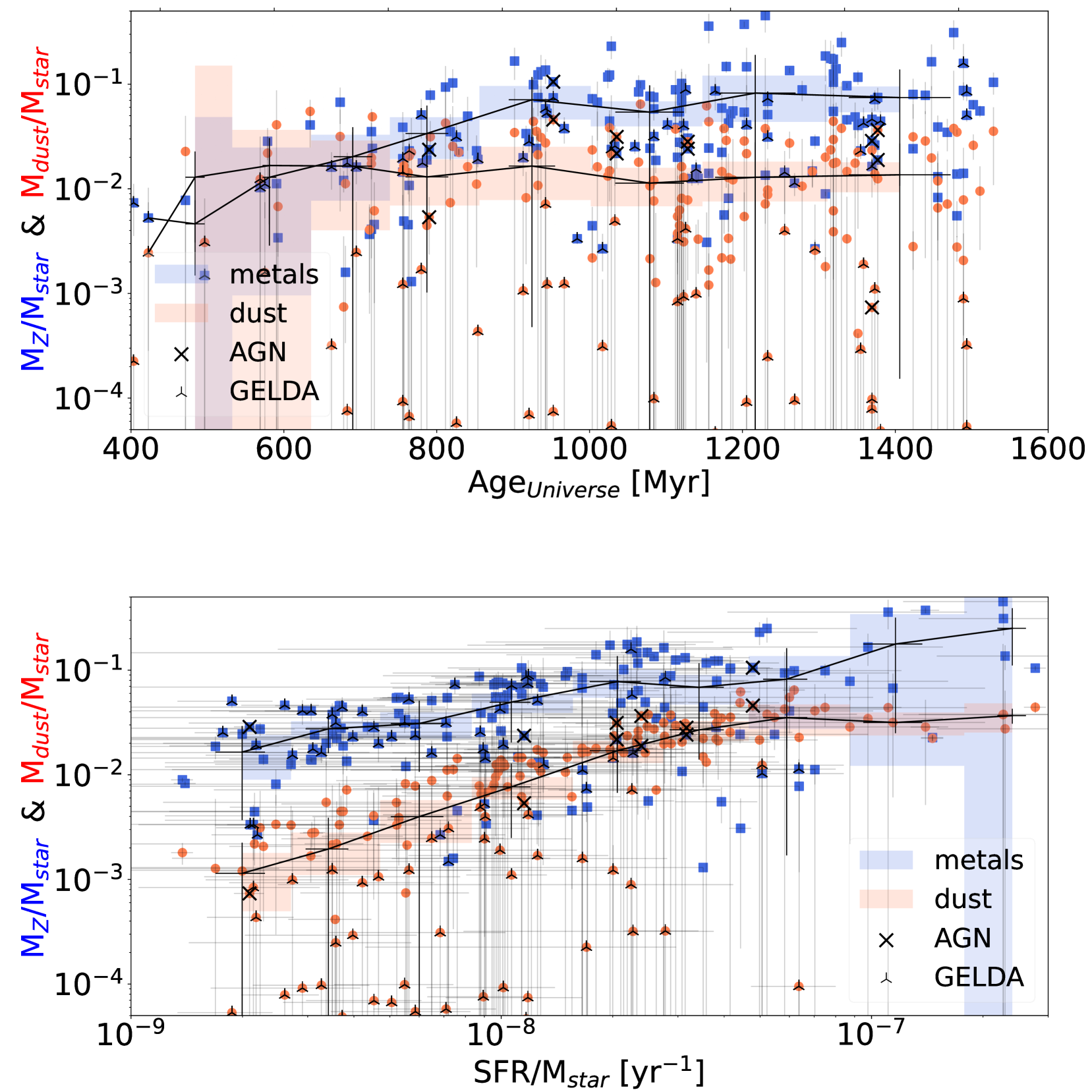
A quantization of the mean dust-to-metal, DTM=¡M_dust/M_Z¿ shown in Fig. 13, gives DTM_mean = 0.080, DTM_median = 0.006 for GELDAs with a first quartile (25 %) Q1 = 0.002 and a third quartile (75 %) Q3 = 0.037, whereas for non GELDAs DTM_mean = 0.654, DTM_median 0.156 with Q1 = 0.085 and Q3 = 0.331. We observe a strong break in the DTM that could be interpreted (Inoue 2011; Asano et al. 2013; Zhukovska 2014; Feldmann 2015; Popping et al. 2017; Hou et al. 2019; Li et al. 2019; Graziani et al. 2020; Triani et al. 2020; Parente et al. 2022; Choban et al. 2024; Dubois et al. 2024) as hints that GELDAs have not started accretion growth of dust while non GELDAs are above the critical metallicity and have dust growth in the ISM. It is interesting to note that Rémy-Ruyer et al. (2014) observed a large scatter in the gas-to-dust mass ratio for a sample of 126 galaxies spanning a 2 dex range in metallicity. This scatter appears at 7.2 $\lesssim 12+\log_{OH}\lesssim$ 8.7 and is consistent with the dust growth in the ISM predicted by Asano et al. (2013) and other works cited in this paper. The objects are those appearing on the bottom left of Fig. 6 and Fig. 13, that is GELDAs. Observations show such a break in the DTM–metallicity relationship at around 0.1 Z_⊙ (Rémy-Ruyer et al. 2014; De Vis et al. 2017) predicted by numerical models (e.g. Popping et al. 2017; Hou et al. 2019; Li et al. 2024; Parente et al. 2022. It is related to the transition in the leading mechanism of dust formation from stardust at low metallicity to ISM growth at high metallicity (Asano et al. 2013; Zhukovska 2014; Popping et al. 2017; Graziani et al. 2020; Li et al. 2019; Lewis et al. 2023.

4 Discussion

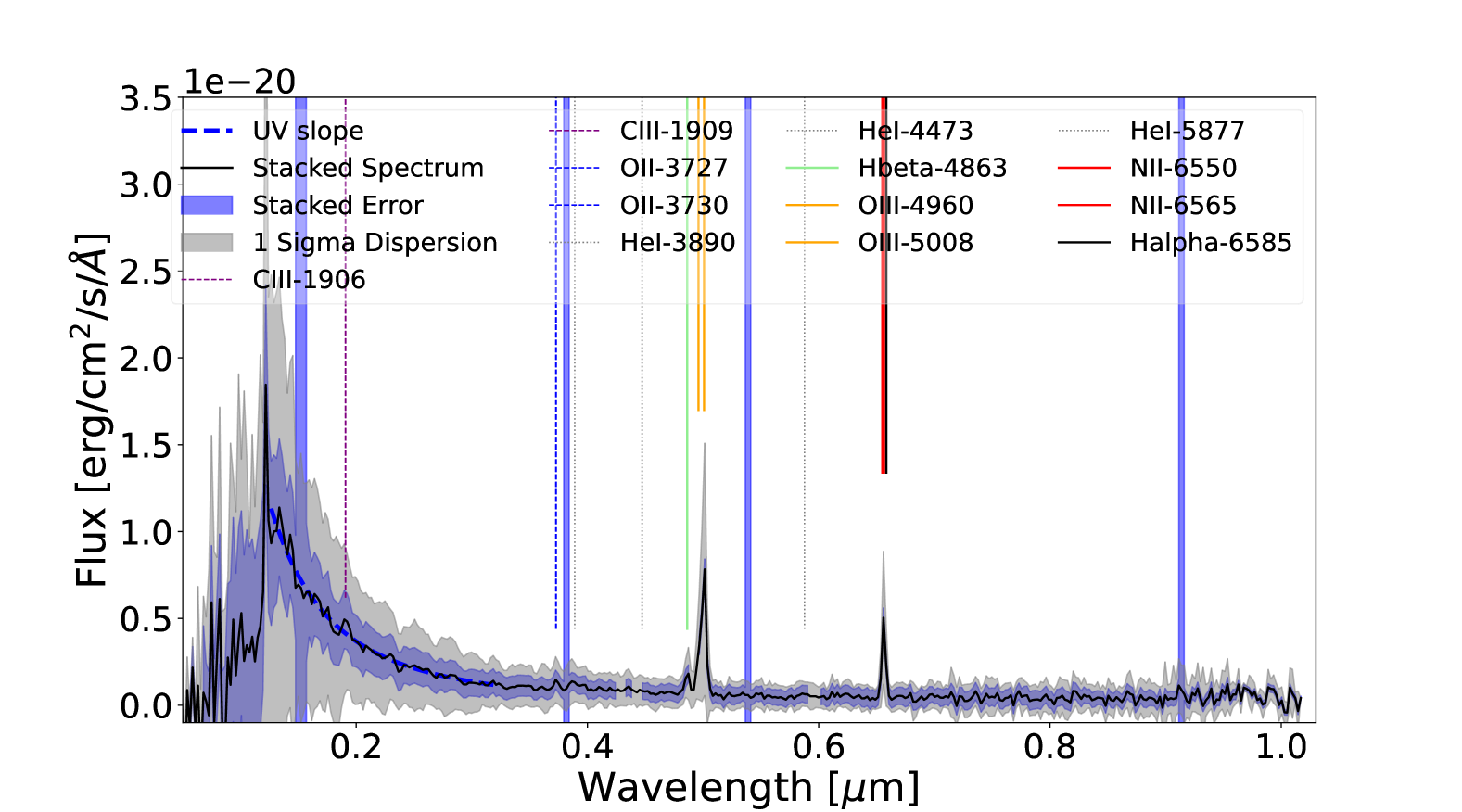
We now analyze the possible origins of GELDAs. To this aim, we first stack the spectra of the GELDAs. See Fig. 14 and line fluxes extracted from the stacked spectrum in Tab. 2. This spectrum is characteristic of star-forming galaxies, with a very blue UV slope $\beta_{FUV}$ = -2.451 $\pm$ 0.066. This sample of GELDAs is compatible with no dust attenuation for Case B: H$\alpha$/H$\beta$=2.932±0.660. To reach H$\alpha$/H$\beta$=2.86 (no dust attenuation), we need to apply a correction to H$\beta$ for the underlying absorption of 2.5 %, a relatively low correction (Kashino et al. 2013; Reddy et al. 2015; Shivaei et al. 2020).

Figure 14: Stacked spectrum of the objects selected in the lower sequence. Vertical lines show the location of a few usual emission lines (see inside caption). We show the position of the lines, including where the HeI lines would be expected. None of them are detected, confirming these objects do not contain a dominant AGN. This stacked spectrum is similar to that of a young starburst, with a blue UV slope and prominent Hydrogen and [OIII) emission lines.

Table 2: Measured UV slope and fluxes of the emission lines of the GELDA stacked spectrum are in erg/cm²/s/$\AA$. We correct the H$\beta$ flux for the underlying absorption that increases H$\beta$ by 2.5 % but we do not correct for H$\alpha$ which is assumed negligible (Kashino et al. 2013; Reddy et al. 2015; Shivaei et al. 2020. With this underlying absorption we would conclude there is no dust attenuation for Case B for these GELDAs.

Parameter	Value
flux CIII $\lambda$1907 $\AA$	$<$ 7.956e-20
flux CIII $\lambda$1909 $\AA$	$<$ 7.956e-20
flux OII $\lambda$3727 $\AA$	$<$ 6.105e-21
flux OII $\lambda$3730 $\AA$	$<$ 6.105e-21
flux OIII $\lambda$4960 $\AA$	7.977E-20 $\pm$ 1.039e-20
flux OIII $\lambda$5008 $\AA$	2.559E-19 $\pm$ 1.039e-20
flux H$\beta$ (measured)	4.850E-20 $\pm$ 1.039e-20
flux H$\beta$ (2.5 % abs.)	4.971e-20 $\pm$ 1.039e-20
flux H$\alpha$	1.422E-19 $\pm$ 9.771e-21
flux NII $\lambda$6550 $\AA$	$<$ 9.771e-21
flux NII $\lambda$6585 $\AA$	$<$ 9.771e-21
$\beta_{FUV}$	-2.451 $\pm$ 0.066
$R_{H}$(F200W)	380 $\pm$ 132 pc
$M_{FUV}$	-18.9 $\pm$ 0.9
$\log_{10}(M_{star}$)	8.36 $\pm$ 0.37

The simplest origin is that these GELDAs are almost unaffected by dust attenuation because they did not produce a significant dust mass. Although this might be possible at z $\gtrsim$ 8.8, this is less likely at lower redshifts because of the global increase in the dust mass density that could pollute gas in the intergalactic medium (e.g. Madau & Dickinson 2014; Traina et al. 2024 or in the average dust attenuation of galaxies (Burgarella et al. 2013; Bogdanoska & Burgarella 2020 from the early Universe to z=3-4. Moreover, some works (e.g. Langeroodi et al. 2024) suggest that dust is formed very fast by SNae on timescales shorter than $\sim 30$ Myr. Even if not all dust grains had been destroyed by the SNae reverse shock, some residual attenuation 0.05 $\leq$ A_V $\leq$ 0.2, which translates to A_FUV = 0.15 - 1.0 depending on the dust attenuation law (Salim & Narayanan 2020), and should still be detectable.

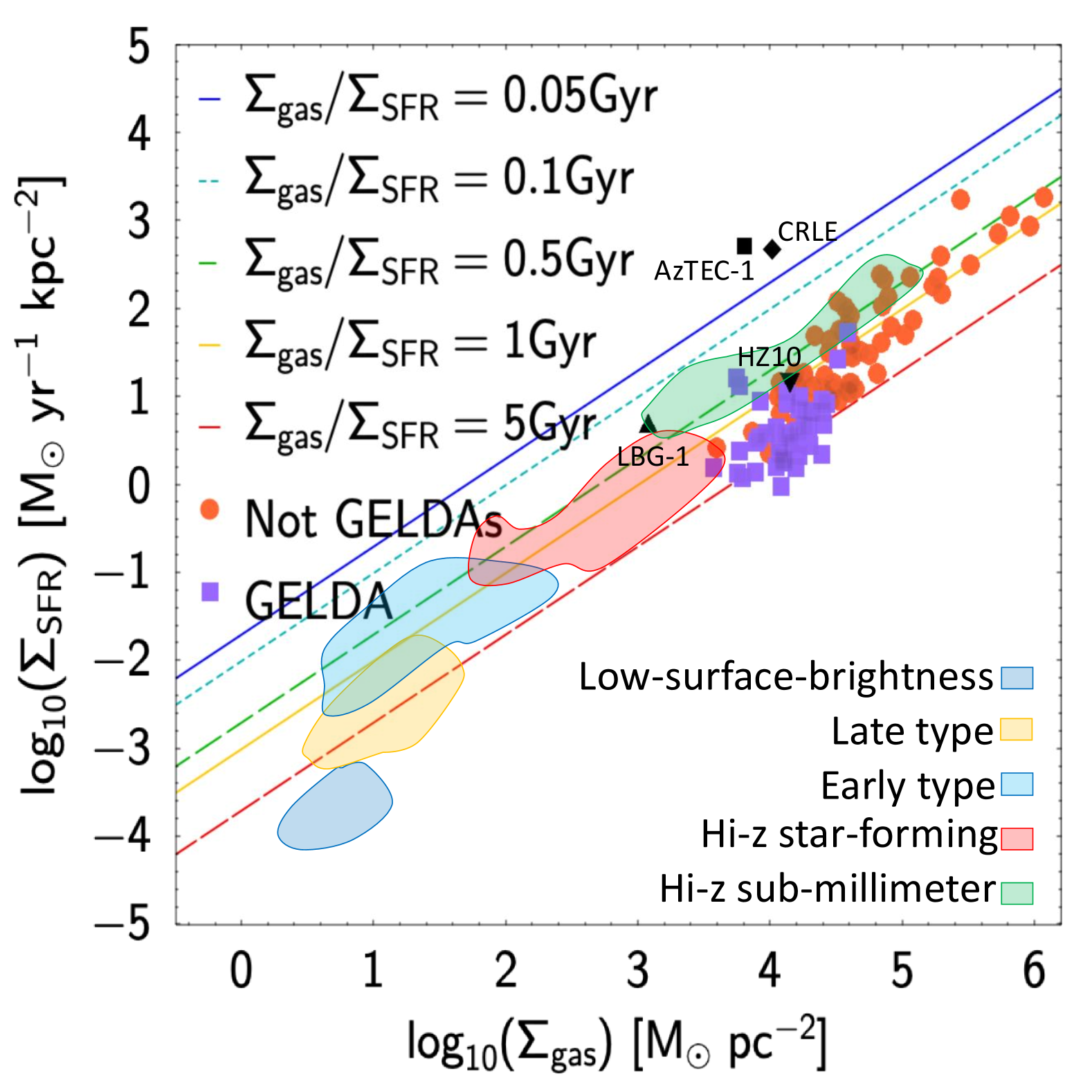
Another origin could be related to the relative geometry of dust and stars in these objects or their small sizes. We know that the brightest H II regions in local galaxies show a correlation between the Balmer line reddening and the dust mass surface density (Kreckel et al. 2013; Trayford et al. 2020; Seillé et al. 2022; Robertson et al. 2024). Our high redshift galaxies are small (Tab. 2). The half-light radii measured in the F200W NIRCam images are $<$RH_F200W$>$ = 380 $\pm$ 132 pc and even less for z $>$ 8.8: $<$RH_F200W$>$ = 327 $\pm$ 87 pc) and thus very dense. We measure the surface densities of gas $0\lesssim\log_{10}(\Sigma_{gas}[M_{\odot}pc^{-2}])\lesssim 6$ and the surface densities of SFR $0\lesssim\log_{10}(\Sigma_{SFR}[M_{\odot}yr^{-1}kpc^{2}]\lesssim 3$. Star formation in galaxies is closely related to the local gas density and follows the so-called Schmidt law (Schmidt 1959). In the dense cores of star formation regions studied in the Milky Way (e.g. Shimajiri et al. 2017; Mattern et al. 2024) and in local spiral galaxies (Gao & Solomon 2004), active high-mass star formation is intimately related to the very dense molecular gas, M_dense. However, when the density of the gas reaches an H₂ surface density $\Sigma_{H2}\gtrsim 100-200\leavevmode\nobreak\ M_{\odot}pc^{-2}$ (Mattern et al. 2024), a density much lower than the estimated values for our galaxies, turbulence can partially prevent star formation because of turbulence and reduce the SFR. This could provide us with an explanation for the location of our sample at low star formation efficiency (SFE), below other objects at the same densities in Fig. 15, offset from both hi-z sub-mm galaxies. These low SFEs are not in agreement with the suggested high FFB-related SFE which is one of the suggested origins of the excess of UV-bright galaxies in the early Universe.

Figure 15: SFR surface density as a function of the gas mass surface density for a sample of local and high-redshift galaxies, including HZ10, LBG-1, AzTEC-3, and CRLE adapted from Pavesi et al. (2019) and Shi et al. (2011). Our objects, GELDAs and not GELDAs are very dense, and all of them are found a bit below other objects, which might be related to the very high gas density in these objects where the turbulence can produce a negative effect on the SFE, which is thus lower than in other high-redshift galaxies at the same gas surface density. The origin of the shaded areas and the correspondence for the symbols are given inside the figure.

A third possible explanation can be found in Ferrara et al. (2023) where they built a model that reproduces the excess of UV-bright galaxies in the luminosity functions at z = 10-14. They propose that these galaxies at z$\gtrsim$11 would contain negligible amounts of dust and that most of the dust produced by SNae in these objects could have been efficiently ejected during the very first phases of galaxy build-up because these galaxies are bursty and they could temporarily evacuate large amounts of gas and dust far from the star-forming region (e.g. Sun et al. 2023; Choban et al. 2024). In this case, the lower objects could correspond to galaxies where dust is efficiently ejected far from the stellar populations by radiation pressure as soon as it is produced by stars. However, if winds had ejected dust in high-redshift galaxies, they probably also expelled gas. However, both for GELDAs and non-GELDAs, we find $f_{gas}=M_{gas}/(M_{gas}+M_{star})$ = 0.96 $\pm$ 0.03 in agreement with models predicting that galaxies with $\log_{10}(M_{star}/M_{\odot})<9.0$ have f${}_{gas}\gtrsim 0.75$ (Davé et al. 2017; Popping et al. 2014). However, galaxies at z $>$ 8.8 have slightly lower but still very high $f_{gas}=0.90\pm 0.05$. Thus, these gas fractions show that these objects still contain a large mass of gas and should therefore also contain dust.

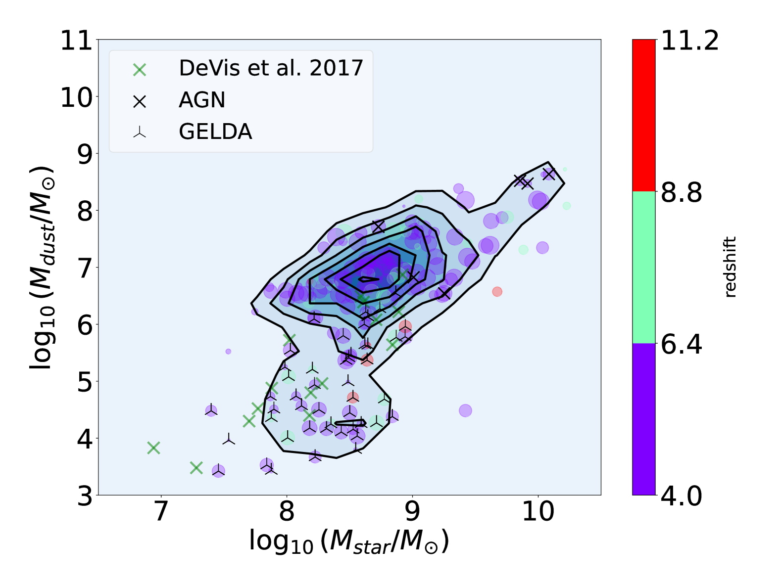
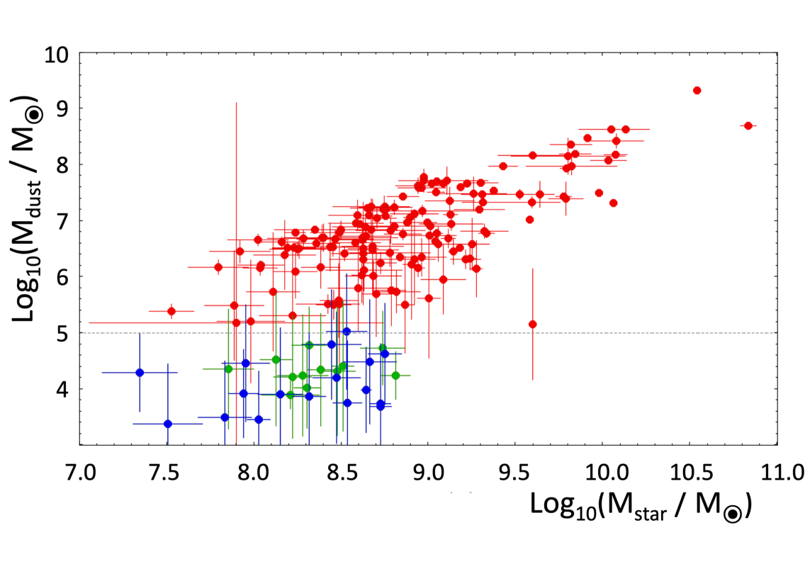
Finally, in the M_dust vs. M_star diagram plotted in Fig. 16, we observe a concentration of galaxies in the upper part of the figure, mainly in the range of 8.0$<$$\log_{10}$(M_star)$<$10.0. We also see a significant decline in dust attenuation at $\log_{10}$(M_star)$\sim$8.0-9.0 that was already seen in Fig. 6. This effect means that M_dust is significantly lower by a factor of 100-1000 at a given stellar mass, with a lower clump or sequence, wel below the upper one. This biphasic plot could suggest a two-mode building of dust mass in galaxies.

Figure 16: M_dust as a function of M_star. Top: The dots are color-coded in redshift. The size of the symbols provides us with information on 12+$\log_{10}$(O/H) with the largest sizes corresponding to the largest metallicities. We show density contours in black, heavy lines. At $\log_{10}$ (M_star) $\sim$ 10^8-9 M_⊙, we observe a transition from an apparent high sequence to a lower one. The upper sequence is similar to that observed at low redshift (e.g. Beeston et al. 2018). The lower objects have not been identified before in this (M_dust vs. M_star) diagram, except for a few objects (green crosses, De Vis et al. 2017). They share the same location in the plot and are extracted from a subsample of galaxies in an HI-selected sample from GAMA and H-ATLAS of local galaxies. Bottom: We plot models on the density contours: the hydrodynamical code dustygadget (Graziani et al. 2020) in yellow, a cosmological hydrodynamical simulation coupled with a chemical evolution model (Mancini et al. 2015) in green and a suite of cosmological, fluid-dynamical simulations of galaxies (Esmerian & Gnedin 2024) in pink. The upper brown line (Witstok et al. 2023) shows where galaxies with ISM-grown grains should be. The bottom orange line corresponds to galaxies with only stardust (Witstok et al. 2023) that underwent a 95 % destruction of grains by reverse SNae shock Witstok et al. 2023). The objects observed at the bottom of the top panel correspond to the transition between galaxies only containing stardust to galaxies dominated by ISM dust.

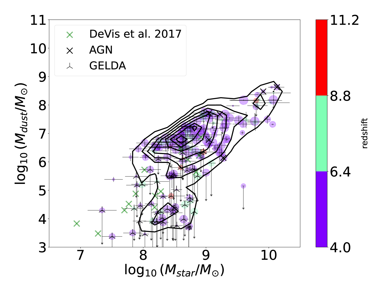
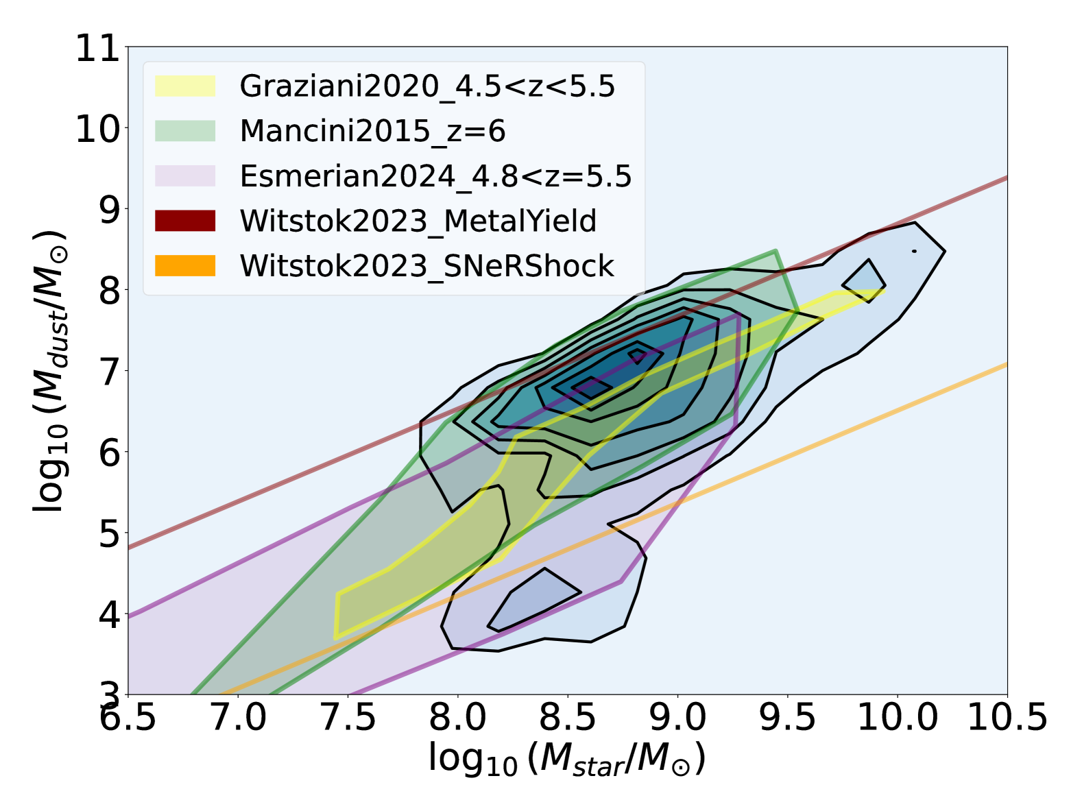
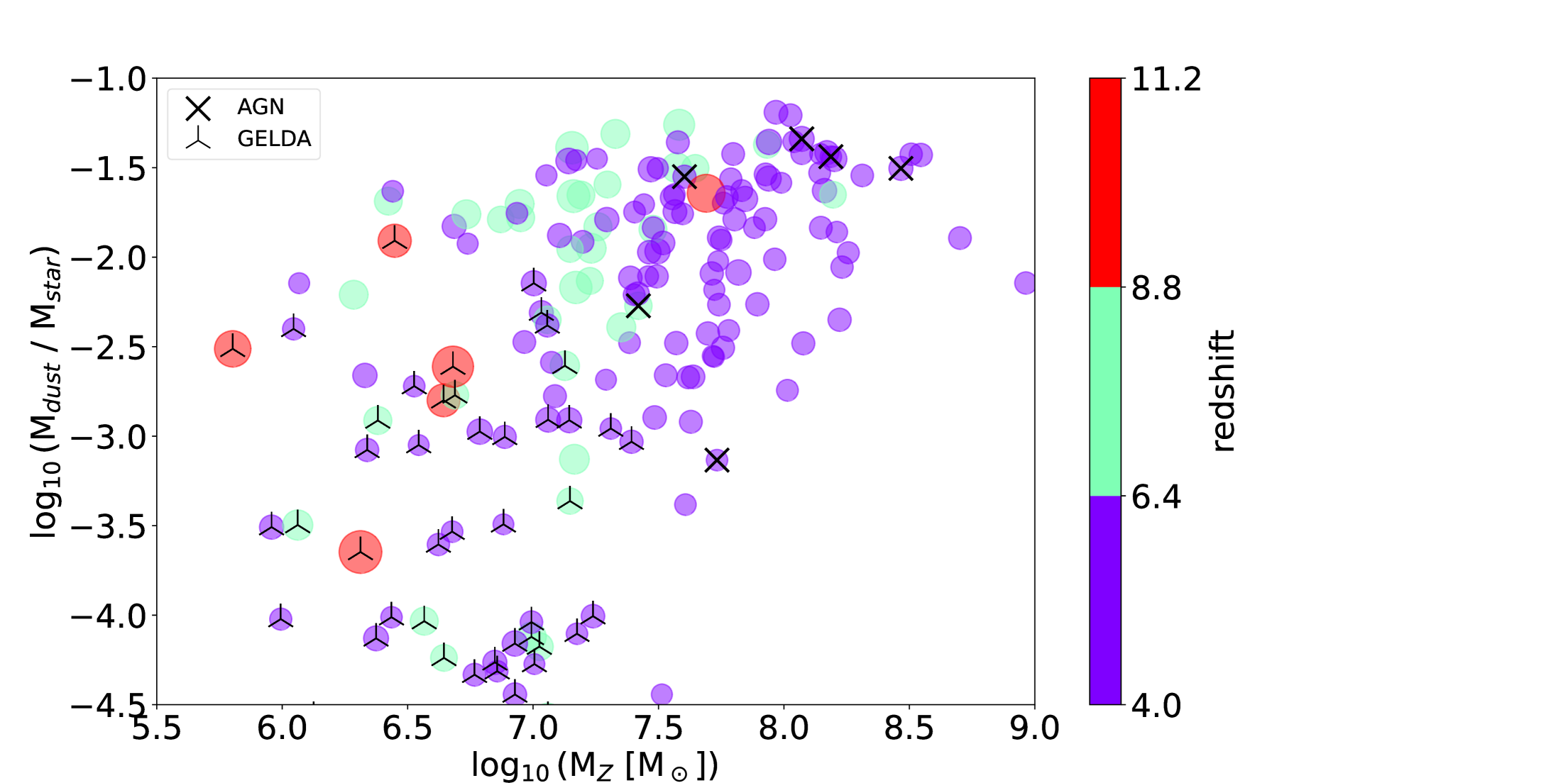
To understand the nature of this lower sequence, Fig. 16 shows several models (Mancini et al. 2015; Graziani et al. 2020; Esmerian & Gnedin 2024; Witstok et al. 2023). The first dust grains should have formed in stellar ejecta from SNae (and maybe AGB stars). However, a possibly substantial fraction of these dust grains is probably destroyed by the SNae reverse shock. After this first phase, the remaining dust grains form seeds and accrete ISM material for grain growth. This process seems to happen only when a critical ISM metallicity is reached at $0.05\lesssim Z/Z_{\odot}\lesssim 0.5$ (Inoue 2011; Asano et al. 2013; Zhukovska 2014; Feldmann 2015; Popping et al. 2017; Hou et al. 2019; Li et al. 2019; Graziani et al. 2020; Triani et al. 2020; Parente et al. 2022; Choban et al. 2024). While the upper sequence would have a dust mass where grains have grown in the ISM, the lower sequence would correspond to stardust grains only formed from SNae, with a grain destruction rate by the SNae reverse shock of the order of 95% (Witstok et al. 2023). The jump from the lower to the upper sequence predicted by the models agrees well with our data. If this population of GELDAs only contains stardust, that we would provide a natural explanation for the excess of UV-bright galaxies at z$<$10 detected by JWST. We check in Figs. 26 and 28 that other assumptions lead to the same apparent transition. Only when no spectroscopic data is used in the fits does the shape of the transition change. Finally, Fig. 17 shows that there are significantly fewer metals in GELDAs compared to the rest of the sample. In this plot, the GELDAs are found in the bottom left of the figure with a metal mass $\log_{10}$(M_Z) $\lesssim$ 7.5 while the sample range extends 5.5 $\lesssim$ $\log_{10}$(M_Z) $\lesssim$ 9.0. This is expected if these objects did not undergo any growth of the dust grains triggered by a larger amount of metals in the ISM because this accretion of ISM material for grain growth is triggered when the metallicity reaches a minimum critical threshold (Asano et al. 2013).

Figure 17: The objects are color-coded in redshift. AGN are shown as crosses and GELDAs are upside-down Y. This figure shows that GELDAs (both z $\geqslant$ 8.8 in red and z $<$ 8.8 in blue) have lower mass of metals than the rest of the sample. This would support the hypothesis that the origin of dust grains in these objects might not be due to ISM growth.

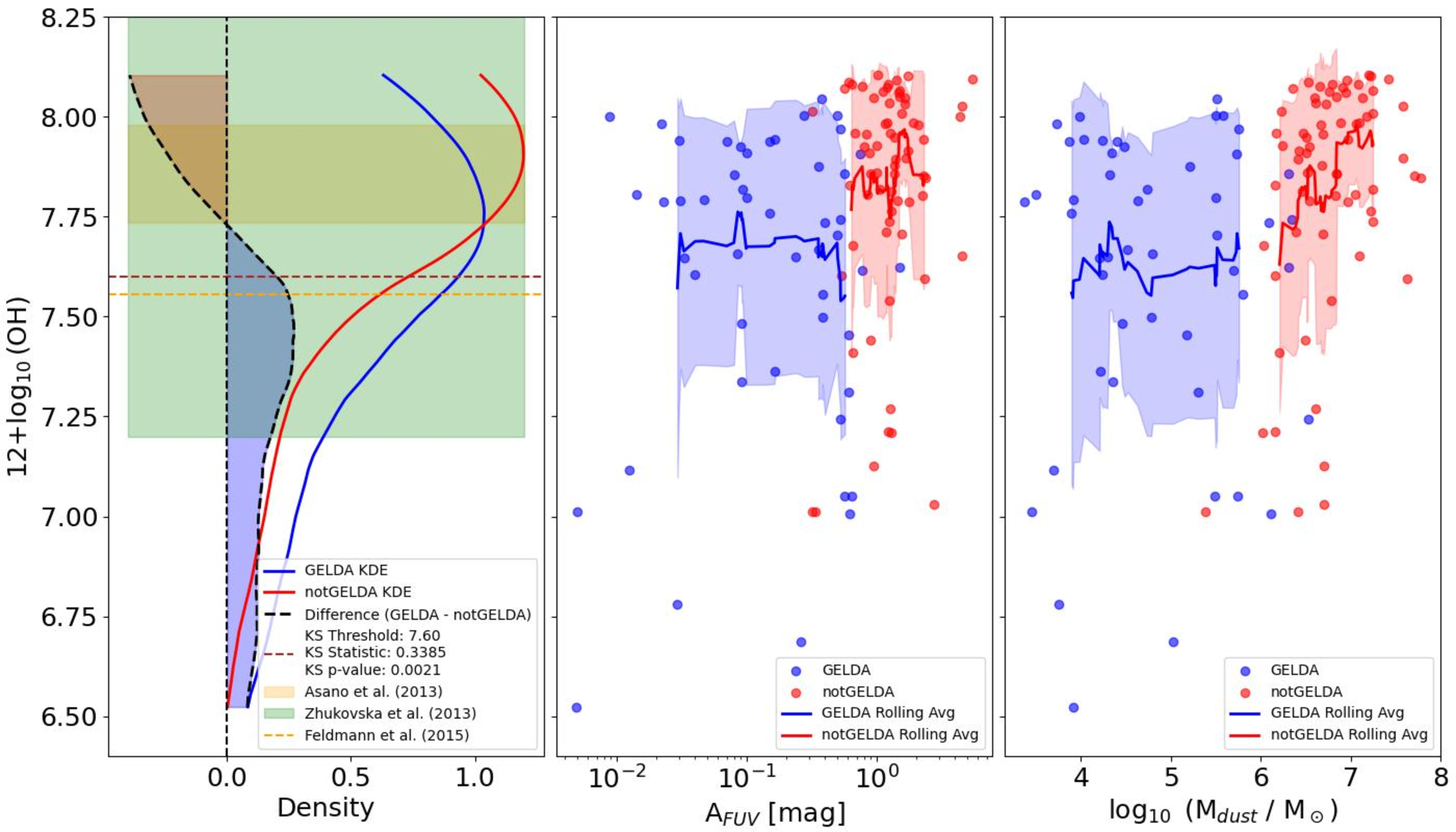
To test whether our hypothesis could be correct, we try to check if we observe a difference in metallicity for GELDAs and not GELDas in Figs. 18. The Kolmogorov-Smirnov (KS) test shown in Fig. 18 suggests that the difference between the two distributions (GELDAs and non-GELDAS) is highly significant. Furthermore, a metallicity threshold is found at 12+$\log_{10}$(O/H)=7.60, which corresponds (with Z_⊙=0.014 and Eq. 1) to Z=0.11. This is in excellent agreement with the critical metallicity (that is, the metallicity at which the contribution of stars equals that of the dust mass growth in the ISM) predicted by the models shown in Fig. 18, in agreement with most models listed in this paper. For example Asano et al. (2013) give: Z/Z_⊙=0.2, that is 12+$\log_{10}$(O/H) = 7.86, and Feldmann et al. (2025) give Z/Z_⊙=0.1, that is 12+$\log_{10}$(O/H) = 7.56.

Figure 18: Distribution of metallicity for GELDAs and not GELDAs. The left panel presents the kernel density estimation (KDE) with an epanechnikov kernel and a bandwidth=0.5 both for GELDAs (blue solid line) and non-GELDAS (red solid line). The black dashed line show the difference. The blue-shaded and red-shaded areas show where GELDAs and non-GELDAs are the dominant population, respectively. We clearly see that GELDAs preferentially cluster at low metallicity, with a threshold estimated at 12+$\log_{10}$(O/H)=7.60. The Kolmogorov-Smirnov confirms that the difference is highly significative. We show predictions for the transition from stardust to ISM from some of the models (see main text for more works): Asano et al. (2013) (orange-shaded area), Zhukovska (2014) (green-shaded area) and Feldmann (2015) (orange dashed line). Rémy-Ruyer et al. (2014) found a larger scatter in their dust-to-gas ratio covers at almost the same metallicity range: 7.2 $\lesssim$ 12+$\log_{10}$(O/H) $\lesssim$ 8.5. All of these metallicities are in good agreement with our estimated threshold. The middle and right panels show the rolling averages (window size=15) of the metallicity as a function of A_FUV and $\log_{10}$ (M_dust). Both panels confirm the difference between GELDAs (blue) and non-GELDAS (red).

The present results provide us with an inherent explanation for the UV-bright tension in the early Universe if these galaxies contain only a low dust mass mainly formed in the circumstellar medium around SNae in the very first phases of star formation and not by accretion in the ISM. This hypothesis is further supported by the fact that in our total sample 5/6 galaxies, that is $\sim$ 83.3 % of the z $\geqslant$ 8.8 galaxies are GELDAs whereas at z $<$ 8.8 only 38/167, that is, 22.8 % are GELDAs, suggesting this type of galaxies could become dominant in the early Universe.

5 Conclusions

We detected a population of galaxies with extremely low dust attenuation (GELDAs) in the redshift range 4.0 $<$ z $<$ 11.4 using a new version of the CIGALE code that accepts both photometric and spectroscopic data. GELDAs are defined as follows:

• A_FUV = 0 within 2$\sigma_{A\_FUV}$, that is no dust attenuation,

• M_star $<$ 10⁹M_⊙

The present galaxy sample shares most of its properties with the ALPINE one in terms of stellar mass: 8.0$\lesssim$M_star$\lesssim$11.4 and redshift: two redshift ranges at 4.40$<$z$<$4.65 and 5.05$<$z$<$5.90 (Burgarella et al. 2022). Assuming that the far-IR dust emission of these GELDAs is similar to that of the ALPINE galaxy sample, we estimate dust masses. In the M_dust vs. M_star diagram, we clearly see a transition at $\log_{10}$(M_star) $\sim$ 8.5 between an upper and a lower sequence. A comparison with models suggests that the transition galaxies could mark the shift from dust solely produced by stellar evolution (stardust galaxies) to dust growth in the ISM of galaxies. The dust-to-metal ratios are very low for GELDAs: DTM${}_{mean}^{GELDA}=0.080$, DTM${}_{median}^{GELDA}=0.006$ with a third quartile Q3 = 0.037 and quite high DTM${}_{mean}^{non-GELDA}=0.654$, DTM${}_{median}^{non-GELDA}=0.156$ with Q3 = 0.331 for non-GELDA, in agreement with the hypothesis of stardust vs. ISM dust.

In our data, a KS test suggests this transition to appear at 12+$\log_{10}$(O/H)=7.60 (Z/Z_⊙=0.1), which is in excellent agreement with the predicted metallicity at which the contribution of stars would equal that of the growth of the dust mass in the ISM in Asano et al. (2013).

The fraction of gas mass $f_{gas}=M_{gas}/(M_{gas}+M_{star})$ $>$ 0.9 for our entire sample of galaxies including GELDAs at all redshifts. This suggests that there is a large gas mass in the galaxies that was not expelled, and supports the hypothesis that dust formed in the galaxies should still remain inside the galaxies.

Finally, the SFE of our galaxies is in agreement with the Schmidt-Kennicutt law (Kennicutt 1998), although at lower SFEs than high-redshift sub-mm galaxies at the same density of gas mass.

In the highest redshift bin at z$>$8.8, almost all galaxies ($\sim$ 83.3 %) can be assigned to the GELDA category, while less than 1/4 of the low-redshift (z$<$8.8) galaxies are GELDAs. These different regimes might mark a transition around z $\sim$ 9. In this highest redshift bin, galaxies with low M_dust/M_star and blue UV slopes contain young, metal-poor stars that may be forming their first dust grains from Pop. II and at z$>$9, possibly Pop. III stars, along with their first metals.

Such stardust galaxies would be ideal suspects to produce the excess of UV-bright galaxies in the early Universe because they might become dominant in the early Universe.

We do not detect any extremely low-metallicity values above z${}_{gas}\sim 10^{-3}$ in our sample of galaxies, and even at z$\gtrsim$8.8, suggesting either a bias in our sample or a rapid rise of metals in the early Universe.

Appendix A Description of the spectro-photometric CIGALE

The concept of CIGALE was developed in the original paper (Burgarella et al. 2005) where multi-wavelength data from the far-UV to the far-IR could be used to derive physical parameters by fitting photometric SEDs. The present open and public version 2025.0, 17 January 2025 of CIGALE (Boquien et al. 2019) is written in Python and parallelized. It also includes a much larger number of modules (that is, physical processes and models) that provide the user with a rich choice to adapt the modeling phase to most galaxies. This Python CIGALE code is also one of the fastest SED fitting codes in the world (Burgarella et al. 2024), making it faster than some of the machine-learning-based codes (namely the convolutional neural network and the deep learning neural network as used in Euclid Collaboration et al. 2023). However, the most important difference of this new version is the possibility to combine spectroscopic data to photometric data (hereafter spectrophotometric data or SPED) with their own uncertainties, while conserving CIGALE’s ability to fit several thousands of objects in a reasonable time. This means that whatever the parameters derived via the fitting process are, these parameters have to be consistent with both photometric and spectroscopic data. Fitting the 173 galaxies using 800 million models from this sample takes about 12 hours on a 48-core computer with 512 GB of memory, utilizing about 60 GB for each run.

In order to combine the two above data types, we have to normalize the spectrum to the photometry. We provide three options: 1) no normalization: raw data are combined, 2) we integrate the modeled spectra into the filters and estimate a global normalization factor through a $\chi^{2}$ when the signal-to-noise ratio $>$5 for the photometric bands used to compute $\chi^{2}$, and 3) we determine a wavelength-dependent normalization. We stress that normalizing the spectroscopic data to the photometric data could be problematic if the emission inside the photometric aperture is physically different from the emission inside the spectral slit. In this case, the resulting fit might not be realistic because of the different natures of the emitting regions. For instance, a dusty galaxy might present a clear region in the outskirts that could dominate the spectrum in UV but not elsewhere in the spectrum if both observations are not at the same position. Converging would thus be difficult, and a good global fit would not be reached. We therefore recommend being careful when combining the spectroscopic and photometric data. For small galaxies like ours, this issue is minimized because we are more likely to observe the same region photometrically and spectroscopically.

In order to simultaneously fit all the data, we need to inform CIGALE about the (sometimes wavelength-dependent) spectral resolution of the spectrometer to create resolution elements corresponding to the instrumental spectral resolution where the models are integrated. This phase is transparent to the user and is performed during the configuration of the CIGALE environment. A typical CIGALE spectrophotometric run appears similar to a photometric run from the user’s point of view.

CIGALE learns that some spectroscopic data have to be taken into account from the configuration file, pcigale.ini, where a specific flag is set to ’True’ as shown in Fig. 19.

Figure 19: This flag must be set to ”True” in the pcigale.ini file to fit spectroscopic data.

Moreover, the input table must contain the following information:

• ”id” that contains an alphanumeric identifier (a different one for each object to be fitted)

• ”redshift” that contains the redshift of the objects or ”NaN” if redshifts have to be estimated.

• ”spectrum” which contains the path to the spectrum

• ”mode” that contains the type of spectrum, e.g. ”prism” if JWST/NIRSpec data is used

• ”norm” where one of the three normalizations should be provided for each object: ”none”, ”global” or ”wave”. Note that the normalization could be different for each object. If no photometric data are given to CIGALE, ”none” should be used, and only the spectrum will be fitted.

Appendix B Parameters used in CIGALE’s final fit

All the spectral models computed by this new version of CIGALE (momentarily dubbed CIGALE-SPEC) using the selected modules (each one corresponding to a physical emission) are convolved with NIRSpec’s prism spectral resolution matched to the observed spectra. The modules and the list of priors are listed in Tab. 3. These spectral data are added to the photometry to form a SPED. The rest of the process follows the usual flow of CIGALE as described in Boquien et al. (2019). The nebular models have been computed with CLOUDY, as described in Theulé et al. (2024). In this analysis, we normalize the prism spectroscopic data by computing a wavelength-dependent normalization, which is estimated from the photometry in the wavelength range, for the photometric bands that have a SNR$>$5.0. A one-dimensional piecewise linear interpolation with given discrete photometric data points is used to derive the wavelength-dependent normalization factor. This normalization is computed for each and every object with photometric data and applied to each spectroscopic observation. In this work, we used the WMAP7 cosmology (Komatsu et al. 2011). We assumed a Chabrier initial mass function (IMF, Chabrier 2003) with lower and upper mass cutoffs M_low = 0.1 M_⊙ and M_up = 100 M_⊙, and a solar metallicity Z_⊙ = 0.014 (Bruzual & Charlot 2003), and the dust emission models, use $\kappa_{\nu}$ = 0.637 m² kg^-2. We show examples of SPED fits in Figs. 20, 22 and 24 over the full spectral range and 21, 23 and 25 over the NIRSpec range.

Figure 20: a) Objects in the upper sequence (larger M_dust) in M_dust vs. M_star plot. We present a sample of spectral fits over the whole spectral range, that is including NIRSpec spectroscopy and the sub-millimeter data (mostly upper limits).

Figure 21: b) Same as Fig. 20 for the same objects but only the fits of the NIRSpec spectrum is shown, which is a zoom in the previous plots.

Figure 22: Same as previous Fig. 20.

Figure 23: Same as Fig. 21.

Figure 24: Objects in the lower sequence (lower M_dust) in M_dust vs. M_star plot. Same as Fig. 20 but for objects in the lower sequence in the M_dust vs. M_star plot.

Figure 25: Same as Fig. 24 for the same objects but only the fits of the NIRSpec spectrum is shown, which is a zoom in the previous plots.

Parameters	Symbol	Run #1	Run #2
Target sample		173 NIRSpec-observed objects	173 NIRSpec-observed objects
Delayed SFH and recent burst
e-folding time scale of the delayed SFH	$\tau_{main}$ [Myr]	500	—
Age of the main population	Agemain[Myr]	2, 5, 10, 25, 50, 250, 500, 1000	—
e-folding time scale of the delayed SFH	$\tau_{burst}$ [Myr]	10000	—
Age of the young population	Ageburst[Myr]	1	—
Periodic SFH
Type of the individual star formation episodes	—	—	delayed
Elapsed time between the beginning of each burst	$\delta_{burst}$ [Myr]	—	10, 50, 100, 250
e-folding time scale of the delayed SFH	$\tau_{burst}$ [Myr]	—	10, 100
Age of the episodes	Age [Myr]	—	1, 5, 10, 50, 100, 200, 400, 600, 800, 1000
SSP
SSP		BC03	BC03
Initial mass function	IMF	Chabrier	Chabrier
Metallicity	Z	0.0001, 0.0004, 0.004, 0.008, 0.02, 0.05	0.0001, 0.0004, 0.004, 0.008, 0.02, 0.05
Nebular emission
Ionization parameter	logU	-1.0, -1.2, -1.4, -1.6, -1.8, -2.0, -2.2, -2.4, -2.6, -2.8, -3.0, -3.2, -3.4, -3.6, -3.8, -4.0	-1.0, -1.2, -1.4, -1.6, -1.8, -2.0, -2.2, -2.4, -2.6, -2.8, -3.0, -3.2, -3.4, -3.6, -3.8, -4.0
Gas metallicity	Zgas	0.0001, 0.0004, 0.001, 0.002, 0.0025, 0.003, 0.004, 0.005	0.0001, 0.0004, 0.001, 0.002, 0.0025, 0.003, 0.004, 0.005
Electron density	nH	10, 100, 1000	10, 100, 1000
Line width [km/s]	—	150	150
Dust attenuation law
Color excess for both the old and young stellar populations	E_BV_lines	1e-4, 0.001, 0.010, 0.050, 0.10, 0.15, 0.20, 0.25, 0.30, 0.50, 0.75, 1.0, 1.5, 2.0, 3.0, 5.0	1e-4, 0.001, 0.010, 0.050, 0.10, 0.15, 0.20, 0.25, 0.30, 0.50, 0.75, 1.0, 1.5, 2.0, 3.0, 5.0
Reduction factor to apply on E_BV_lines to compute E(B-V)s the stellar continuum attenuation.	E_BV_factor	0.44	0.44
Bump amplitude	uv_bump_amplitude	0.0	0.0
Power law slope	power law_slope	-0.6, -0.30, 0.0, 0.30, 0.6	-0.6, -0.30, 0.0, 0.30, 0.6
Dust emission (DL2014)
Mass fraction of PAH	$q_{PAH}$	0.47	0.47
Minimum radiation field	Umin	17.0	17.0
Power law slope dU/dM $\approx$ Uα	$\alpha$	2.4	2.4
Dust fraction in PDRs	$\gamma$	0.54	0.54
No AGN emission

Table 3: CIGALE modules and input parameters used for all the fits. BC03 means Bruzual & Charlot (2003), and the Chabrier IMF refers to Chabrier (2003).

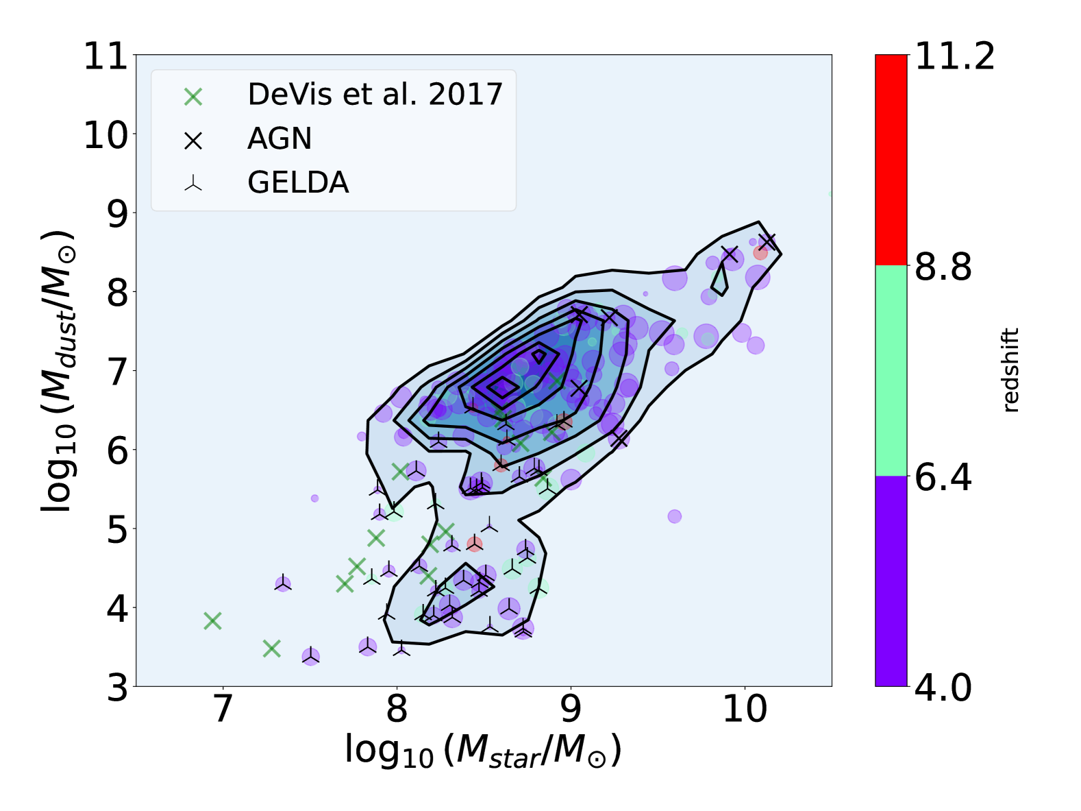
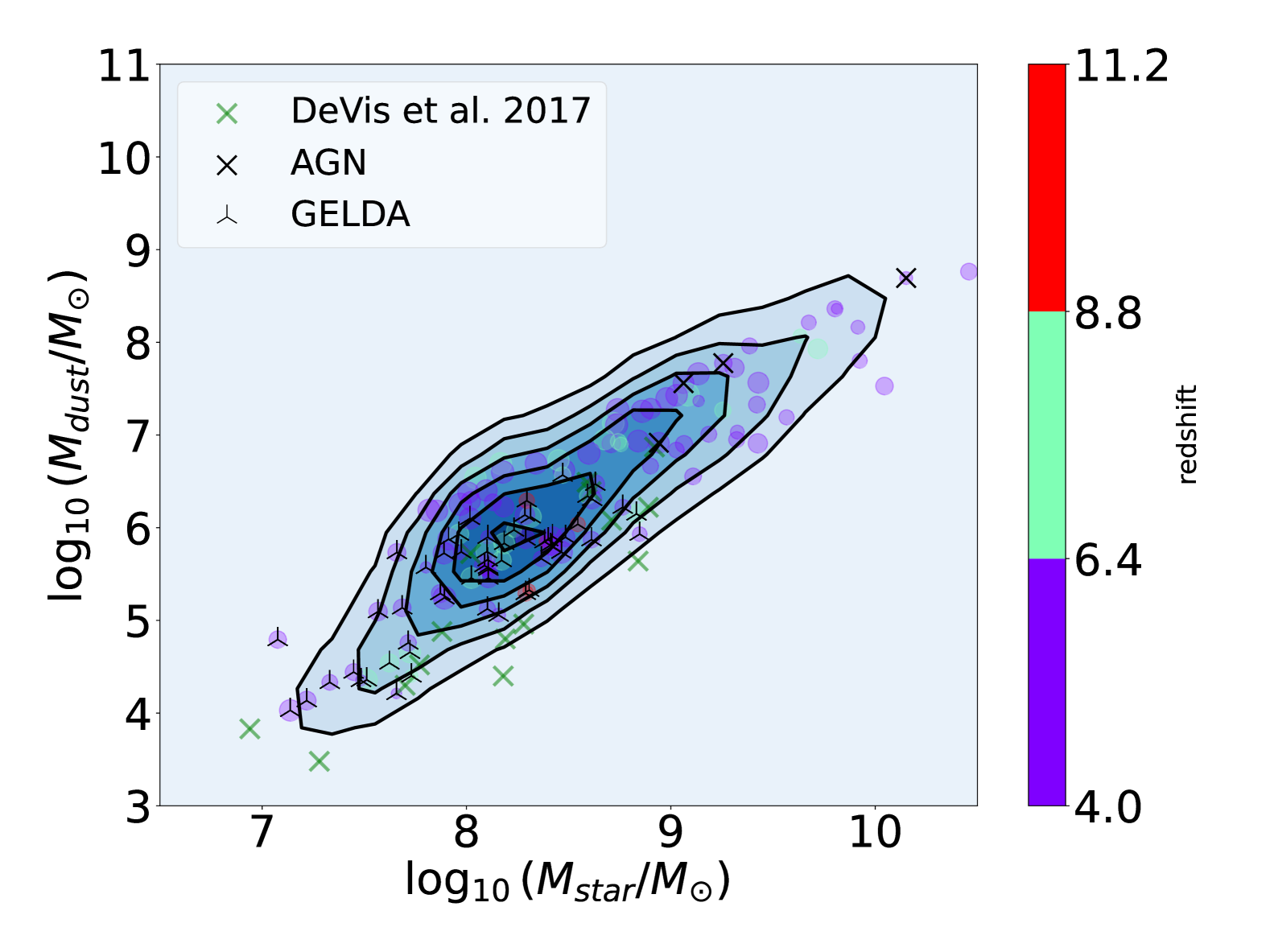
Appendix C Results assuming a periodic star formation history

We present the same analysis obtained in the main paper, but here, we assume a periodic SFH, that is, a series of regular bursts over the age of galaxies (Fig. 27). The main parameters that define the SFH for this CIGALE run are listed in Tab. 3. The conclusions presented in the main article could also be reached with a periodic SFH, confirming that the type of SFH does not fundamentally impact the results of the article. To also test if the wavelength range or the type of data (photometric or spectroscopic) could influence the results presented in this paper, we also present the same M_dust vs. M_star diagram in Fig. 28: while we do not observe any meaningful differences in the top panel if we do not use the sub-mm data, the two sequences detected in Fig. 16 disappear in the bottom panel, showing that the information from the spectrum is fundamental for identifying the stardust and ISM dust sequences.

Figure 26: This figure is the same as Fig. 6. However, for this one we assume a periodic SFH. This alternate version allows to reach the same conclusion than Fig. 6, with a population of GELDAs.

Figure 27: This figure is the same as Fig. 16. However, for this one we assume a periodic SFH. This alternate version also allows to reach the same conclusion than Fig. 6, with a population of GELDAs.

Figure 28: Test on the stability of the results with the type of data used: Top - This figure is created by fitting the spectrophotometric data, as in Fig. 16 and Fig. 27, except that we do not use the sub-mm ones. The trend observed in this case is almost identical, which confirms the less important role of the sub-mm data in separating the two parallel sequences. Bottom - This figure is created by only fitting the photometric data, including the sub-mm ones but not the spectroscopic one. The trend observed in this case is different from when we make use of the NIRSpec spectra. We still do see a small decrease at lower stellar mass, even though the less-marked downturn suggests that without spectroscopy, some strong spectral information, and especially the line ratios, is missing. However, the photometric data still bring an information on the dust attenuation because of the UV slope $\beta_{FUV}$. The correlation of $\beta_{FUV}$ with the dust mass is much less significant, and leads to this smaller difference in dust mass, even at low stellar masses which makes the second lower sequence less prominent.

References

- Akins et al. (2023) Akins, H. B., Casey, C. M., Allen, N., et al. 2023, ApJ, 956, 61
- Algera et al. (2024a) Algera, H. S. B., Inami, H., De Looze, I., et al. 2024a, MNRAS, 533, 3098
- Algera et al. (2024b) Algera, H. S. B., Inami, H., Sommovigo, L., et al. 2024b, MNRAS, 527, 6867
- Arrabal Haro et al. (2023) Arrabal Haro, P., Dickinson, M., Finkelstein, S. L., et al. 2023, ApJ, 951, L22
- Asano et al. (2013) Asano, R. S., Takeuchi, T. T., Hirashita, H., & Inoue, A. K. 2013, Earth, Planets and Space, 65, 213
- Atek et al. (2023) Atek, H., Shuntov, M., Furtak, L. J., et al. 2023, MNRAS, 519, 1201
- Bagley et al. (2023) Bagley, M. B., Finkelstein, S. L., Koekemoer, A. M., et al. 2023, ApJ, 946, L12
- Beeston et al. (2018) Beeston, R. A., Wright, A. H., Maddox, S., et al. 2018, MNRAS, 479, 1077
- Béthermin et al. (2020) Béthermin, M., Fudamoto, Y., Ginolfi, M., et al. 2020, A&A, 643, A2
- Birkmann et al. (2022) Birkmann, S. M., Ferruit, P., Giardino, G., et al. 2022, A&A, 661, A83
- Bogdanoska & Burgarella (2020) Bogdanoska, J. & Burgarella, D. 2020, MNRAS, 496, 5341
- Boquien et al. (2019) Boquien, M., Burgarella, D., Roehlly, Y., et al. 2019, A&A, 622, A103
- Bouwens et al. (2016) Bouwens, R. J., Aravena, M., Decarli, R., et al. 2016, ApJ, 833, 72
- Bruzual & Charlot (2003) Bruzual, G. & Charlot, S. 2003, MNRAS, 344, 1000
- Burgarella et al. (2022) Burgarella, D., Bogdanoska, J., Nanni, A., et al. 2022, A&A, 664, A73
- Burgarella et al. (2024) Burgarella, D., Buat, V., Boquien, M., Roehlly, Y., & Lambert, J.-C. 2024, in Society of Photo-Optical Instrumentation Engineers (SPIE) Conference Series, Vol. 13098, Observatory Operations: Strategies, Processes, and Systems X, ed. C. R. Benn, A. Chrysostomou, & L. J. Storrie-Lombardi, 130980N
- Burgarella et al. (2013) Burgarella, D., Buat, V., Gruppioni, C., et al. 2013, A&A, 554, A70
- Burgarella et al. (2005) Burgarella, D., Buat, V., & Iglesias-Páramo, J. 2005, MNRAS, 360, 1413
- Casey et al. (2024) Casey, C. M., Akins, H. B., Shuntov, M., et al. 2024, ApJ, 965, 98
- Chabrier (2003) Chabrier, G. 2003, PASP, 115, 763
- Chakraborty et al. (2024) Chakraborty, P., Sarkar, A., Wolk, S., et al. 2024, arXiv e-prints, arXiv:2406.05306
- Choban et al. (2024) Choban, C. R., Kereš, D., Sandstrom, K. M., et al. 2024, MNRAS, 529, 2356
- Chowdhury et al. (2022) Chowdhury, A., Kanekar, N., & Chengalur, J. N. 2022, ApJ, 935, L5
- Cole et al. (2025) Cole, J. W., Papovich, C., Finkelstein, S. L., et al. 2025, ApJ, 979, 193
- Davé et al. (2017) Davé, R., Rafieferantsoa, M. H., Thompson, R. J., & Hopkins, P. F. 2017, MNRAS, 467, 115
- Dayal et al. (2022) Dayal, P., Ferrara, A., Sommovigo, L., et al. 2022, MNRAS, 512, 989
- De Vis et al. (2017) De Vis, P., Dunne, L., Maddox, S., et al. 2017, MNRAS, 464, 4680
- Dell’Agli et al. (2019) Dell’Agli, F., Valiante, R., Kamath, D., Ventura, P., & García-Hernández, D. A. 2019, MNRAS, 486, 4738
- Di Cesare et al. (2023) Di Cesare, C., Graziani, L., Schneider, R., et al. 2023, MNRAS, 519, 4632
- Draine et al. (2014) Draine, B. T., Aniano, G., Krause, O., et al. 2014, ApJ, 780, 172
- Dubois et al. (2024) Dubois, Y., Rodríguez Montero, F., Guerra, C., et al. 2024, A&A, 687, A240
- Esmerian & Gnedin (2024) Esmerian, C. J. & Gnedin, N. Y. 2024, ApJ, 968, 113
- Euclid Collaboration et al. (2023) Euclid Collaboration, Bisigello, L., Conselice, C. J., et al. 2023, MNRAS, 520, 3529
- Feldmann (2015) Feldmann, R. 2015, MNRAS, 449, 3274
- Feldmann et al. (2025) Feldmann, R., Boylan-Kolchin, M., Bullock, J. S., et al. 2025, MNRAS, 536, 988
- Fernández et al. (2024) Fernández, V., Amorín, R., Firpo, V., & Morisset, C. 2024, A&A, 688, A69
- Ferrara et al. (2023) Ferrara, A., Pallottini, A., & Dayal, P. 2023, MNRAS, 522, 3986
- Ferrara et al. (2025) Ferrara, A., Pallottini, A., & Sommovigo, L. 2025, A&A, 694, A286
- Ferrara et al. (2022) Ferrara, A., Sommovigo, L., Dayal, P., et al. 2022, MNRAS, 512, 58
- Finkelstein et al. (2023) Finkelstein, S. L., Bagley, M. B., Ferguson, H. C., et al. 2023, ApJ, 946, L13
- Finkelstein et al. (2024) Finkelstein, S. L., Leung, G. C. K., Bagley, M. B., et al. 2024, ApJ, 969, L2
- Fudamoto et al. (2017) Fudamoto, Y., Ivison, R. J., Oteo, I., et al. 2017, MNRAS, 472, 2028
- Gao & Solomon (2004) Gao, Y. & Solomon, P. M. 2004, ApJ, 606, 271
- Graziani et al. (2020) Graziani, L., Schneider, R., Ginolfi, M., et al. 2020, MNRAS, 494, 1071
- Grieco et al. (2023) Grieco, F., Theulé, P., De Looze, I., & Dulieu, F. 2023, Nature Astronomy, 7, 541
- Grogin et al. (2011) Grogin, N. A., Kocevski, D. D., Faber, S. M., et al. 2011, ApJS, 197, 35
- Groves et al. (2012) Groves, B., Brinchmann, J., & Walcher, C. J. 2012, MNRAS, 419, 1402
- Harikane et al. (2023) Harikane, Y., Zhang, Y., Nakajima, K., et al. 2023, ApJ, 959, 39
- Heintz et al. (2023a) Heintz, K. E., Giménez-Arteaga, C., Fujimoto, S., et al. 2023a, ApJ, 944, L30
- Heintz et al. (2023b) Heintz, K. E., Shapley, A. E., Sanders, R. L., et al. 2023b, A&A, 678, A30
- Hezaveh et al. (2015) Hezaveh, Y. D., Marshall, P. J., & Blandford, R. D. 2015, ApJ, 799, L22
- Hirashita et al. (2014) Hirashita, H., Ferrara, A., Dayal, P., & Ouchi, M. 2014, MNRAS, 443, 1704
- Hopkins et al. (2018) Hopkins, P. F., Wetzel, A., Kereš, D., et al. 2018, MNRAS, 480, 800
- Hou et al. (2019) Hou, K.-C., Aoyama, S., Hirashita, H., Nagamine, K., & Shimizu, I. 2019, MNRAS, 485, 1727
- Hutter et al. (2025) Hutter, A., Cueto, E. R., Dayal, P., et al. 2025, A&A, 694, A254
- Ilie et al. (2023) Ilie, C., Paulin, J., & Freese, K. 2023, Proceedings of the National Academy of Science, 120, e2305762120
- Inami et al. (2022) Inami, H., Algera, H. S. B., Schouws, S., et al. 2022, MNRAS, 515, 3126
- Inoue (2011) Inoue, A. K. 2011, Earth, Planets and Space, 63, 1027
- Iyer et al. (2019) Iyer, K. G., Gawiser, E., Faber, S. M., et al. 2019, ApJ, 879, 116
- Jeong et al. (2025) Jeong, T. B., Jeon, M., Song, H., & Bromm, V. 2025, ApJ, 980, 10
- Kashino et al. (2013) Kashino, D., Silverman, J. D., Rodighiero, G., et al. 2013, ApJ, 777, L8
- Kennicutt (1998) Kennicutt, Jr., R. C. 1998, ApJ, 498, 541
- Kocevski et al. (2023) Kocevski, D. D., Onoue, M., Inayoshi, K., et al. 2023, ApJ, 954, L4
- Koekemoer et al. (2011) Koekemoer, A. M., Faber, S. M., Ferguson, H. C., et al. 2011, ApJS, 197, 36
- Komatsu et al. (2011) Komatsu, E., Smith, K. M., Dunkley, J., et al. 2011, ApJS, 192, 18
- Kreckel et al. (2013) Kreckel, K., Groves, B., Schinnerer, E., et al. 2013, ApJ, 771, 62
- Langeroodi et al. (2024) Langeroodi, D., Hjorth, J., Ferrara, A., & Gall, C. 2024, arXiv e-prints, arXiv:2410.14671
- Laporte et al. (2017) Laporte, N., Ellis, R. S., Boone, F., et al. 2017, ApJ, 837, L21
- Larson et al. (2023) Larson, R. L., Finkelstein, S. L., Kocevski, D. D., et al. 2023, ApJ, 953, L29
- Lei et al. (2025) Lei, L., Wang, Y.-Y., Yuan, G.-W., et al. 2025, ApJ, 980, 249
- Leja et al. (2019) Leja, J., Carnall, A. C., Johnson, B. D., Conroy, C., & Speagle, J. S. 2019, ApJ, 876, 3
- Leśniewska & Michałowski (2019) Leśniewska, A. & Michałowski, M. J. 2019, A&A, 624, L13
- Lewis et al. (2023) Lewis, J. S. W., Ocvirk, P., Dubois, Y., et al. 2023, MNRAS, 519, 5987
- Li et al. (2019) Li, Q., Narayanan, D., & Davé, R. 2019, MNRAS, 490, 1425
- Li et al. (2024) Li, Z., Dekel, A., Sarkar, K. C., et al. 2024, A&A, 690, A108
- Lower et al. (2020) Lower, S., Narayanan, D., Leja, J., et al. 2020, ApJ, 904, 33
- Lower et al. (2023) Lower, S., Narayanan, D., Li, Q., & Davé, R. 2023, ApJ, 950, 94
- Madau & Dickinson (2014) Madau, P. & Dickinson, M. 2014, ARA&A, 52, 415
- Mancini et al. (2015) Mancini, M., Schneider, R., Graziani, L., et al. 2015, MNRAS, 451, L70
- Mattern et al. (2024) Mattern, M., André, P., Zavagno, A., et al. 2024, A&A, 688, A163
- Mauerhofer & Dayal (2023) Mauerhofer, V. & Dayal, P. 2023, MNRAS, 526, 2196
- Messias et al. (2024) Messias, H., Guerrero, A., Nagar, N., et al. 2024, MNRAS, 533, 3937
- Naidu et al. (2022) Naidu, R. P., Oesch, P. A., van Dokkum, P., et al. 2022, ApJ, 940, L14
- Nakajima et al. (2023) Nakajima, K., Ouchi, M., Isobe, Y., et al. 2023, ApJS, 269, 33
- Nakajima et al. (2022) Nakajima, K., Ouchi, M., Xu, Y., et al. 2022, ApJS, 262, 3
- Nanni et al. (2020) Nanni, A., Burgarella, D., Theulé, P., Côté, B., & Hirashita, H. 2020, A&A, 641, A168
- Nicholls et al. (2017) Nicholls, C. P., Lebzelter, T., Smette, A., et al. 2017, A&A, 598, A79
- Palla et al. (2024) Palla, M., De Looze, I., Relaño, M., et al. 2024, MNRAS, 528, 2407
- Parente et al. (2022) Parente, M., Ragone-Figueroa, C., Granato, G. L., et al. 2022, MNRAS, 515, 2053
- Pavesi et al. (2019) Pavesi, R., Riechers, D. A., Faisst, A. L., Stacey, G. J., & Capak, P. L. 2019, ApJ, 882, 168
- Popping et al. (2017) Popping, G., Somerville, R. S., & Galametz, M. 2017, MNRAS, 471, 3152
- Popping et al. (2014) Popping, G., Somerville, R. S., & Trager, S. C. 2014, MNRAS, 442, 2398
- Pozzi et al. (2021) Pozzi, F., Calura, F., Fudamoto, Y., et al. 2021, A&A, 653, A84
- Reddy et al. (2015) Reddy, N. A., Kriek, M., Shapley, A. E., et al. 2015, ApJ, 806, 259
- Rémy-Ruyer et al. (2014) Rémy-Ruyer, A., Madden, S. C., Galliano, F., et al. 2014, A&A, 563, A31
- Robertson et al. (2024) Robertson, C., Holwerda, B. W., Young, J., et al. 2024, AJ, 167, 263
- Salim & Narayanan (2020) Salim, S. & Narayanan, D. 2020, ARA&A, 58, 529
- Sanders et al. (2024) Sanders, R. L., Shapley, A. E., Topping, M. W., Reddy, N. A., & Brammer, G. B. 2024, ApJ, 962, 24
- Schmidt (1959) Schmidt, M. 1959, ApJ, 129, 243
- Seillé et al. (2022) Seillé, L. M., Buat, V., Haddad, W., et al. 2022, A&A, 665, A137
- Shi et al. (2011) Shi, Y., Helou, G., Yan, L., et al. 2011, ApJ, 733, 87
- Shimajiri et al. (2017) Shimajiri, Y., André, P., Braine, J., et al. 2017, A&A, 604, A74
- Shivaei et al. (2022) Shivaei, I., Popping, G., Rieke, G., et al. 2022, ApJ, 928, 68
- Shivaei et al. (2020) Shivaei, I., Reddy, N., Rieke, G., et al. 2020, ApJ, 899, 117
- Sommovigo et al. (2022a) Sommovigo, L., Ferrara, A., Carniani, S., et al. 2022a, MNRAS, 517, 5930
- Sommovigo et al. (2022b) Sommovigo, L., Ferrara, A., Pallottini, A., et al. 2022b, MNRAS, 513, 3122
- Speagle et al. (2014) Speagle, J. S., Steinhardt, C. L., Capak, P. L., & Silverman, J. D. 2014, ApJS, 214, 15
- Strandet et al. (2017) Strandet, M. L., Weiss, A., De Breuck, C., et al. 2017, ApJ, 842, L15
- Sun et al. (2023) Sun, G., Faucher-Giguère, C.-A., Hayward, C. C., & Shen, X. 2023, MNRAS, 526, 2665
- Tacchella et al. (2023) Tacchella, S., Johnson, B. D., Robertson, B. E., et al. 2023, MNRAS, 522, 6236
- Tacconi et al. (2020) Tacconi, L. J., Genzel, R., & Sternberg, A. 2020, ARA&A, 58, 157
- Tamura et al. (2019) Tamura, Y., Mawatari, K., Hashimoto, T., et al. 2019, ApJ, 874, 27
- Theulé et al. (2024) Theulé, P., Burgarella, D., Buat, V., et al. 2024, A&A, 682, A119
- Traina et al. (2024) Traina, A., Magnelli, B., Gruppioni, C., et al. 2024, A&A, 690, A84
- Trayford et al. (2020) Trayford, J. W., Lagos, C. d. P., Robotham, A. S. G., & Obreschkow, D. 2020, MNRAS, 491, 3937
- Triani et al. (2020) Triani, D. P., Sinha, M., Croton, D. J., Pacifici, C., & Dwek, E. 2020, MNRAS, 493, 2490
- Valentino et al. (2024) Valentino, F., Fujimoto, S., Giménez-Arteaga, C., et al. 2024, A&A, 685, A138
- Valiante et al. (2009) Valiante, R., Schneider, R., Bianchi, S., & Andersen, A. C. 2009, MNRAS, 397, 1661
- Vieira et al. (2013) Vieira, J. D., Marrone, D. P., Chapman, S. C., et al. 2013, Nature, 495, 344
- Vijayan et al. (2019) Vijayan, A. P., Clay, S. J., Thomas, P. A., et al. 2019, MNRAS, 489, 4072
- Walter et al. (2020) Walter, F., Carilli, C., Neeleman, M., et al. 2020, ApJ, 902, 111
- Watson et al. (2015) Watson, D., Christensen, L., Knudsen, K. K., et al. 2015, Nature, 519, 327
- Weibel et al. (2024) Weibel, A., Oesch, P. A., Barrufet, L., et al. 2024, MNRAS, 533, 1808
- Witstok et al. (2023) Witstok, J., Jones, G. C., Maiolino, R., Smit, R., & Schneider, R. 2023, MNRAS, 523, 3119
- Yung et al. (2024) Yung, L. Y. A., Somerville, R. S., Finkelstein, S. L., Wilkins, S. M., & Gardner, J. P. 2024, MNRAS, 527, 5929
- Zackrisson et al. (2011) Zackrisson, E., Rydberg, C.-E., Schaerer, D., Östlin, G., & Tuli, M. 2011, ApJ, 740, 13
- Zavala et al. (2018) Zavala, J. A., Aretxaga, I., Dunlop, J. S., et al. 2018, MNRAS, 475, 5585
- Zavala et al. (2023) Zavala, J. A., Buat, V., Casey, C. M., et al. 2023, ApJ, 943, L9
- Zhukovska (2014) Zhukovska, S. 2014, A&A, 562, A76
- Zhukovska et al. (2018) Zhukovska, S., Henning, T., & Dobbs, C. 2018, ApJ, 857, 94