Hadamard product in deep learning:
Introduction, Advances and Challenges

Abstract

While convolution and self-attention mechanisms have dominated architectural design in deep learning, this survey examines a fundamental yet understudied primitive: the Hadamard product. Despite its widespread implementation across various applications, the Hadamard product has not been systematically analyzed as a core architectural primitive. We present the first comprehensive taxonomy of its applications in deep learning, identifying four principal domains: higher-order correlation, multimodal data fusion, dynamic representation modulation, and efficient pairwise operations. The Hadamard product’s ability to model nonlinear interactions with linear computational complexity makes it particularly valuable for resource-constrained deployments and edge computing scenarios. We demonstrate its natural applicability in multimodal fusion tasks, such as visual question answering, and its effectiveness in representation masking for applications including image inpainting and pruning. This systematic review not only consolidates existing knowledge about the Hadamard product’s role in deep learning architectures but also establishes a foundation for future architectural innovations. Our analysis reveals the Hadamard product as a versatile primitive that offers compelling trade-offs between computational efficiency and representational power, positioning it as a crucial component in the deep learning toolkit.

1 Introduction

Deep neural networks (DNNs) have demonstrated unparalleled success in learning complicated concepts. Diverse tasks (such as image classification [1], image generation [2, 3], image inpainting [4, 5], language understanding [6, 7], sequence modeling [8, 9], sequence transduction [10] and multimodal learning [11, 12]) are nowadays predominantly modelled with DNNs. One of the pillars behind the success of DNNs (and the focus of this work) is the choice of the architectural components, and more specifically the type of correlations captured.

Two of the most popular architectural components used across domains and tasks are the convolutional layer and the self-attention [10]. A convolutional layer represents an element as a weighted sum of the neighboring input elements. Concretely, given a datapoint $\bm{Z}$ (e.g., a sequence of text tokens or an image), a convolutional layer expresses each output as $\sum_{i,j}w_{i,j}z_{i,j}$ for (learnable) weights $\bm{W}$. A convolutional layer captures linear correlations between the input elements, which limits the contextual information. On the contrary, the self-attention (SA) represents nonlinear interactions through a matrix multiplication of the input elements, i.e., products of the form $(\bm{W}_{1}\bm{Z})\cdot(\bm{W}_{2}\bm{Z})$ for (learnable) weights $\bm{W}_{1},\bm{W}_{2}$. However, SA suffers from a quadratic computational cost over the number of input elements [13], which results in a significant computational overhead for deep networks. Instead, the Hadamard product captures nonlinear interactions with a linear computational cost. The Hadamard product is a pairwise operator that accepts two input tensors and outputs their element-by-element product in each position. Representing nonlinear interactions with a linear computational cost is critical in the era of deep networks, e.g., in order to use them on edge devices [14, 15] or especially for large language models and foundational models [16] that are computationally intensive.

TABLE I: Recent works using the Hadamard product. Beyond the seminal works that Hadamard product has been used, the Hadamard product exists in new applications, e.g., in recent language models or parameter-efficient fine-tuning.

Category	Task	Method	Publication
High-order interactions	Video action recognition	[17]	ICCV’23
	Image classification	MONet [18]	ICLR’24
	Masked language modeling	M2 [19]	NeurIPS’23
	Classification/segmentation	RMT [20]	CVPR’24
Multimodal fusion	Video Question Answering	[21]	CVPR’24
	Image generation	MultiDiffusion [22]	ICML’23
	Image generation	DenseDiffusion [23]	ICCV’23
Adaptive modulation	Language modeling	xLSTM [8]	NeurIPS’24
	Classification/segmentation	V-RWKV [24]	ICLR’25
	Pruning	PX [25]	CVPR’24
	3D texture generation	[26]	ICCV’23
	Conditional image generation	LayoutFlow [27]	ECCV’24
	Language modeling	[28]	NeurIPS’24
	Language modeling	Mamba [29]	COLM’24
	Language modeling	Mamba2 [30]	ICML’24
	Language modeling	HGRN2 [31]	COLM’24
	Language modeling	GLA [32]	ICML’24
Efficient operator	Image classification	Poly-SA [33]	PAMI’23
	Image classification	StarNet [34]	CVPR’24
	Masked language modeling	FLASH [15]	ICML’22
	Parameter-efficient fine-tuning	LoHa [35]	ICLR’22
	Parameter-efficient fine-tuning	HiRA [36]	ICLR’25
	Parameter-efficient fine-tuning	MLAE [37]	Arxiv, May’24

Capturing nonlinear interactions is especially important when we have different modalities. As humans, we perceive the world through various sensory input, e.g., visual and auditory modalities, that offer complementary information, while they share a common underlying structure. Enabling neural networks to process and understand multimodal information is critical for important applications, such as medical analysis. Clearly, data from different modalities might vary widely in volume, making processing more difficult. A core part of processing multimodal data is the fusion of those volumes. A way to fuse information is through naive concatenation, however this expresses only linear interactions [38]. Richer, nonlinear interactions can be captured with tensor decompositions, such as the popular CP decomposition. If we use the CP decomposition, the Hadamard product emerges naturally through standard properties (cf. the mixed product [39] or Lemma 2). Naturally, the Hadamard product has been widely applied to multimodal fusion tasks, such as in visual question answering [11] or multimodal medical analysis [40].

Beyond the linear computational cost and the multimodal fusion, we argue that the Hadamard product lies at the heart of deep learning (DL) with far-reaching applications. In this work, our aim is to contextualize those applications of the Hadamard product and to frame it as a core operator in deep learning. Concretely, our analysis focuses on four categories where the Hadamard product has been instrumental. The first category revolves around representing high-order correlations, e.g., as in StyleGAN [2] or SENet [1]. The second category develops the fusion of multimodal data, where different communities have independently used the Hadamard product as a fusion scheme. Then, we present the use of Hadamard product for dynamic filtering of features, e.g., in case there are corrupted parts of the image in masking [4, 5], and dynamic modulation of the weights, e.g., in Dropout to avoid overfitting or in LSTM to avoid vanishing/exploding gradients [8]. Masking is also utilized in language modeling, e.g., with linear attention models [41], to enable efficient training on text sequences. This is critical for more computationally efficient training of models predicting the next output token. The last category we revisit the computational efficiency of the Hadamard product, e.g., for reducing the complexity of standard self-attention blocks. By linking these applications of the Hadamard product and presenting them in a unified perspective, we hope to provide a more comprehensive understanding of this important operator in deep learning. This could also help to connect seemingly unrelated components, such as the inductive bias of polynomial networks [42] and the inductive bias of LSTM. In Table I we review some recent works in each category, with additional, significant works being mentioned in the respective sections, e.g., Tables II and III. All in all, the contributions of this survey are the following:

• This work presents the first taxonomy of the Hadamard product, establishing significant connections among different categories, such as multimodal fusion and high-order interactions.

• Within each category, we explore how various concepts influence the application of the Hadamard product, for example, masking in adaptive modulation.

• We highlight the key theoretical properties of the Hadamard product that have been developed in isolation. We discuss the impact of these properties, such as the effect of spectral bias on high-order interactions.

• We identify important open problems in Section 7, which are expected to stimulate future research on this topic.

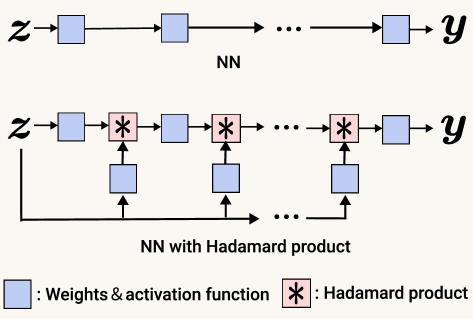
(a) High-order interactions: Regular NN (top) and how to include higher-order interactions (bottom)

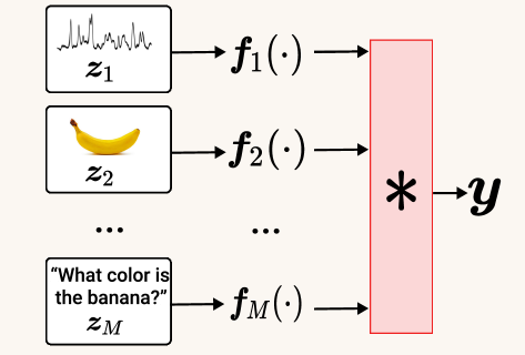
(b) Multimodal Fusion

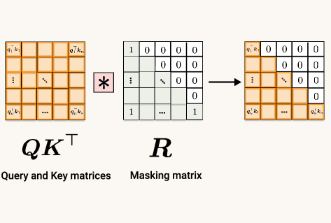
(c) Adaptive modulation: Casual language modeling with linear attention

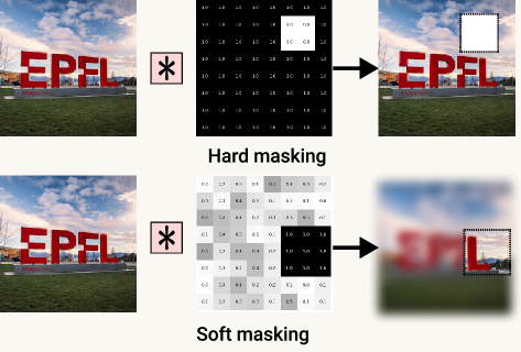
(d) Adaptive modulation: Hard masking (top) and soft masking (bottom)

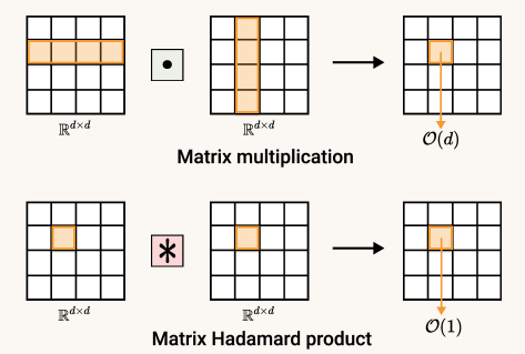
(e) Efficient operator

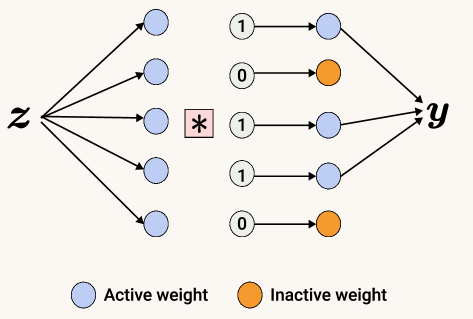
(f) Adaptive modulation and efficient operator: Weight pruning

Figure 1: Six core areas where the Hadamard product has been widely used in deep learning era. (a) High-order correlations between the input elements are captured. Those correlations can augment the linear interactions of the typical layers, e.g., dense or convolutional layers. (b) As humans we generally perceive the world through different senses, which often offer complementary information. Similarly, machine learning (ML) models can extract complementary information from different sources and then meld them together to make an informed decision. (c) During the pre-training of language modeling, we mask attention to the key of future tokens for each query so that the model does not use information from the next token when predicting the next token. (d) Hard masking and soft masking via Hadamard product for the image in the input space. (e) The Hadamard product has recently been used as an alternative operator to the matrix multiplication, e.g., in order to accelerate the popular Self-Attention. (f) Weight pruning can be viewed as applying a Hadamard product to the original weights, effectively zeroing out certain parameters. Among those core areas, we identify four parent categories and links between them (e.g. weight pruning). To our knowledge, this taxonomy is novel and allows us to establish concrete connections between seemingly disparate works within the same category, such as masking for inpainting and causal language modeling. To facilitate further research, we have also compiled the diverse open-source links in Table S4.

Brief history: The term Hadamard product was originally termed in [43]. The influential book of [44] argues that the most popular references attribute the first use of this product in the manuscripts of Jacques Hadamard [45, 46]. However, more recent books [47] argue that this element-wise product had actually emerged at least few years earlier in Moutard’s work. The works of Hadamard and Schur [48] are among the first to (re-)invent the element-wise product. A by-product of the numerous re-inventions of this product is that there is no universally accepted symbol for the Hadamard product [47]. In this work, we will interchangeably use the term Hadamard and element-wise product, while we denote this product with the symbol ‘$*$’.

Relationship to other surveys: The rise in deep learning components and tasks has led to numerous surveys, covering areas like attention networks [49], recurrent networks [50], Dropout [51], tensors [39, 52, 53], and multimodal learning [54]. While the Hadamard product is related to some of these topics, such as Dropout and multimodal fusion, it is not the primary focus of these surveys. Our work fills this gap by explicitly addressing the Hadamard product and its wide range of applications, complementing existing surveys.

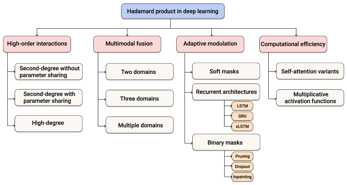
Figure S2: Taxonomy of Hadamard product in deep learning. The category of high-order interactions is often divided by the degree of interactions, with a more fine-grained taxonomy being whether there is parameter-sharing, i.e., Eq. 2 vs Eq. NCP. Similarly, in multimodal fusion, the number of domains is a fundamental separation, with techniques such as VQA belonging to two domains. We believe in the following years, works will increasingly focus on multiple domains for general applications, which simulates how humans perceive and process multiple domains.

Paper outline: We cover the first application of the Hadamard product in deep learning in Section 2, while we provide a verbose taxonomy in Fig. S2. Concretely, the Hadamard product is used there for capturing high-order correlations among the input elements, e.g., expressing a synthesized image as high-order correlations between the elements of the noise vector. This is a topic that has become relevant the last few years following the success of StyleGAN and other similar works. Another major area of research in the Hadamard product is the feature fusion, especially in the context of multimodal learning. We cover various feature fusion schemes using the Hadamard product in Section 3. A third area of development of networks with the Hadamard product is in masking, e.g., as in inpainting or Dropout. The idea is to modulate the input/features, such that the network can (exclusively) focus on certain areas of the representation. This idea has also been explored in the form of gating, which selects dynamically the critical features. Both masking and the gating mechanisms are detailed in Section 4. Furthermore, the Hadamard product has been featured recently as a more (computationally) efficient operator over the more costly matrix multiplication (e.g. in the context of self-attention) as covered in Section 5. Six popular applications of the four parent categories are visually depicted in Fig. 1. Beyond the technical and computational aspects covered, the Hadamard product results in a number of interesting theoretical properties, which are studied in Section 6. Lastly, we conduct a thorough discussion on the benefits of the Hadamard product, as well as highlight existing limitations and identify interesting avenues for future research on the topic in Section 7.

Notation: Matrices (vectors) are denoted by uppercase (lowercase) boldface letters e.g., $\bm{X}$, ($\bm{x}$). Tensors are denoted with boldface, calligraphic letters, e.g., $\bm{\mathcal{X}}$. Detailed notation, along with core mathematical properties appear in Section S.1. In this work, the input to the network is denoted with (vector) $\bm{z}$ or (matrix) $\bm{Z}$.

Definition 1.1 (Hadamard product)

The Hadamard product between two tensors $\bm{\mathcal{X}},\bm{\mathcal{Y}}$ is denoted as $(\bm{\mathcal{X}}*\bm{\mathcal{Y}})\in\mathbb{R}^{I_{1}\times I_{2}\times\cdots\times I_{M}}$ and is defined as

$$(\bm{\mathcal{X}}*\bm{\mathcal{Y}})_{i_{1},i_{2},\ldots,i_{M}}\doteq(\bm{\mathcal{X}})_{i_{1},i_{2},\ldots,i_{M}}\cdot(\bm{\mathcal{Y}})_{i_{1},i_{2},\ldots,i_{M}}\;.$$

Notice that the Hadamard product between vectors and matrices are special cases of this definition. Although the Hadamard product requires that the two tensors share the same dimensions, each $I_{i}$ can be different from $I_{j}$ for $i\neq j$. Further information on tensors, tensor decompositions and products can be found in the classic review papers of [39, 52], while [53] provides a recent overview of tensor in deep learning.

2 High-order interactions

Beyond the linear interactions used in neural networks, polynomial expansions have been explored for approximating signals with unknown analytic expressions. The Stone-Weierstrass theorem [55] guarantees that any smooth function can be approximated by a polynomial expansion, with its multivariate extension covered in standard textbooks, e.g., in [56] (pg 19). In this section, we analyze how such a polynomial expansion can be used to augment the linear interactions of the typical layers used in DNNs. Let $\bm{z}\in\mathbb{R}^{d}$ denote the input, e.g., an image patch, and let $\bm{y}\in\mathbb{R}^{o}$ be the target, e.g., a class label. A polynomial expansion of the input $\bm{z}$ can be considered for approximating the target $\bm{y}$. That is, a vector-valued function ${f}(\bm{z}):\mathbb{R}^{d}\to\mathbb{R}^{o}$ expresses the multivariate polynomial expansion of degree $N$:

$$\bm{y}={f}(\bm{z})=\sum_{n=1}^{N}\bigg{(}\bm{\mathcal{W}}^{[n]}\prod_{j=2}^{n+1}\times_{j}\bm{z}\bigg{)}+\bm{\beta}\;,$$ (1)

where $\bm{\beta}\in\mathbb{R}^{o}$ and $\big{\{}\bm{\mathcal{W}}^{[n]}\in\mathbb{R}^{o\times\prod_{m=1}^{n}\times_{m}d}\big{\}}_{n=1}^{N}$ are the learnable parameters. The form of Eq. 1 can approximate smooth functions (for large $N$). The number of parameters required to accommodate high-order interactions of the input increases exponentially with the desired degree of the polynomial which is impractical for high-dimensional data. Therefore, a form of parameter reduction is applied to each work to make polynomial expansions practical.

Group Method of Data Handling (GMDH) [57] was one of the first works to learn quadratic polynomials. To reduce the parameteres, GMDH defines a predetermined set of interactions between the input elements. The method was later extended in high-degree polynomials [58]. Contrary to the aforementioned predefined interactions, quadratic [59, 60] and high-degree expansions [61, 62] have been learned in a data-driven fashion. In particular, pi-sigma networks [63] use a single multiplicative unit over the input elements. That is, given an input $\bm{z}\in\mathbb{R}^{d}$ the output $\bm{y}\in\mathbb{R}^{o}$ in pi-sigma networks can be expressed as $\bm{y}=\sigma(*_{j=1}^{J}\bm{h}_{j})$, with $\sigma$ an element-wise activation function and $J$ the order of the interactions. The vector $\bm{h}_{j}$ represents the $j^{\text{th}}$ column-vector of the hidden representation $\bm{H}=\bm{\mathcal{W}}\times_{3}\bm{z}+\bm{B}$. The parameters $\bm{\mathcal{W}}\in\mathbb{R}^{o\times J\times d},\bm{B}\in\mathbb{R}^{o\times J}$ are learnable.

More recently, there are a number of works that use polynomial expansions in ML. Various quadratic polynomials of the form $f_{1}(\bm{z})+f_{2}(\bm{z})*f_{3}(\bm{z})$ for appropriate functions of $f_{1},f_{2},f_{3}$ are used in [64, 65, 66, 6, 67, 68, 69, 70, 71, 72, 18, 20]. For instance, in the Gated Linear Unit (GLU) [73], they assume $f_{1}(\bm{z})=\bm{0},f_{2}(\bm{z})=\bm{W}\bm{z}$ and $f_{3}(\bm{z})=\sigma(\bm{V}\bm{z})$ for learnt weights $\bm{W},\bm{V}$. In Highway networks [64] the functions $f_{1}(\bm{z})=\bm{z},f_{2}(\bm{z})=\bm{z}-H(\bm{z})$ and $f_{3}(\bm{z})=\sigma(\bm{W}\bm{z})$ are used.

Beyond second-order interactions, polynomial expansions of arbitrary degree have been introduced, which propose various ways to reduce the parameters of Eq. 1. A straightforward solution is to assume a low-rank structure in each of the tensors. The CP decomposition along with Lemma 2 is used to obtain the output $\bm{y}$ as an $N^{\text{th}}$ degree expansion [74]:

$$\begin{split}\bm{y}=\bm{\beta}+\bm{C}_{1,[1]}^{T}\bm{z}+\Big{(}\bm{C}_{1,[2]}^{T}\bm{z}\Big{)}*\Big{(}\bm{C}_{2,[2]}^{T}\bm{z}\Big{)}+\ldots+\\ \underbrace{\Big{(}\bm{C}_{1,[N]}^{T}\bm{z}\Big{)}*\ldots*\Big{(}\bm{C}_{N,[N]}^{T}\bm{z}\Big{)}}_{\text{N Hadamard products}}\;,\end{split}$$ (2)

where $\{\bm{C}_{i,[j]}\in\mathbb{R}^{d\times o}\}_{i,j=1}^{N}$ are learnable parameters. The index $i$ in the matrices $\bm{C}_{i,[j]}$ corresponds to the $i^{\text{th}}$ term in the $j^{\text{th}}$ order interactions. This expression reduces the learnable parameters significantly from exponential to ${\Theta}(N^{2}\cdot d\cdot o)$.

We can reduce further the parameters by assuming that certain factors are shared across different layers. The sharing can be achieved by jointly factorizing all the tensors $\{\bm{\mathcal{W}}^{[n]}\}_{n=1}^{N}$. In $\Pi$-Net [75], various such concrete coupled tensor decompositions are utilized to jointly factorize the tensors. A simple recursive expression of that factorization is exhibited below:

$$\bm{y}_{n}=\left(\bm{A}_{[{n}]}^{T}\bm{z}\right)*\left(\bm{S}_{[{n}]}^{T}\bm{y}_{n-1}+\bm{b}_{[{n}]}\right)\;,$$ (NCP)

for $n=2,\ldots,N$ with $\bm{y}_{1}=\Big{(}\bm{A}_{[{1}]}^{T}\bm{z}\Big{)}*\bm{b}_{[{1}]}$ and $\bm{y}=\bm{C}\bm{y}_{N}+\bm{\beta}$. The parameters $\bm{C}\in\mathbb{R}^{o\times k},\bm{A}_{[{n}]}\in\mathbb{R}^{d\times k},\bm{S}_{[{n}]}\in\mathbb{R}^{k\times k}$, $\bm{b}_{[{n}]}\in\mathbb{R}^{k}$ for $n=1,\ldots,N$, are learnable with $k\in\mathbb{N}$ the rank of the decomposition. That is, the final output $\bm{y}$ is an $N^{\text{th}}$ degree polynomial expansion of the input $\bm{z}$ and is obtained as an affine transformation of the last recursive term $\bm{y}_{N}$. The recursive terms $\{\bm{y}_{n}\}_{n=1}^{N}$ provide the intermediate representations. Eq. NCP includes few core operations that exist in all major deep learning frameworks and as such, it can be easily implemented. An indicative implementation of Eq. NCP is added in Section S.2.2. Note that the learnable parameters are of the order $\Theta(N\cdot d\cdot o)$ owing to the parameters sharing. The recursive formula is obtained by assuming a hierarchical CP decomposition with shared factors as illustrated in [75], while different recursive formulations can be obtained if we change the assumptions or the factorization of the terms.

In practice, there are two relaxations over the formulations above: Firstly, often activation functions are used in between the different terms for stabilizing the training [75]. Secondly, the aforementioned polynomial expansions are often used as polynomial layers, which are then composed sequentially to obtain the final network. For instance, the second polynomial layer of Eq. NCP accepts the output of the first polynomial layer of Eq. NCP as input. That is, the final network is a composition of the polynomial layers. The total degree of expansion is then the product of the degrees of each polynomial layer. The benefit of such a composition is that it can increase the total degree of expansion without increasing the number of layers significantly. For instance, a product of $N$ polynomial layers of degree $2$ results in a $2^{N}$ total degree.

Let us now demonstrate two additional applications of the aforementioned polynomial expansion of Eq. NCP. Fathony et al. [76] apply an elementwise function $g$ on the output of the term $\left(\bm{A}_{[{n}]}^{T}\bm{z}\right)$ of Eq. NCP. They consider two special forms of functions $g$, i.e., the sinusoid and the Gabor filter. In both cases, they illustrate that the final output is a linear combination of Fourier or Gabor bases respectively. Follow-up works further extend the types of filters and add constraints to those [77, 78]. The idea is to use such networks for approximating low-dimensional functions, e.g., given an $(x,y)$ coordinate of an input image output the RGB values of that coordinate. This implicit representation task has been frequently met across a range of domains, such as computer vision, the last few years.

The second application concerns the influential work of StyleGAN [2]. In StyleGAN, a Hadamard-based generator is introduced for the first time in the Generative Adverarial Nets (GANs) [79]. The Hadamard product is performed in the ADAIN layer [80], while the generator structure resembles Eq. NCP. The authors illustrate how this structure leads to an unsupervised separation of high-level attributes. Follow-up works [81, 82] have further focused on the disentanglement of the high-level attributes using the inductive bias of the Hadamard product.

Besides the vector-based analysis above, a tailored analysis could be performed depending on the type of data/task. The seminal squeeze-and-Excitation block (SENet) [1] relies on an image structure. The output captures pairwise channel correlations of the input $\bm{Z}\in\mathbb{R}^{hw\times c}$, where $h$ denotes the height, $w$ the width and $c$ the channels of the image. Notation-wise, the output $\bm{Y}$ is expressed as:

$$\bm{Y}=(\bm{Z}\bm{C}_{{}_{[{1}]}})*r(p(\bm{Z}\bm{C}_{{}_{[{1}]}})\bm{C}_{{}_{[{2}]}})\;.$$ (3)

The functions $p,r$ represent the global pooling and the replication of the spatial dimensions respectively. The matrices $\bm{C}_{{}_{[{1}]}}\in\mathbb{R}^{c\times\omega},\bm{C}_{{}_{[{2}]}}\in\mathbb{R}^{\omega\times c}$ are learnable. The output of the global pooling $p(\bm{Z}\bm{C}_{{}_{[{1}]}})$ is a vector of size $\omega$. Follow-up works have extended the pairwise channel correlations [83, 84, 85]. Indicatively, the selective kernel nets [86] perform a minor re-parametrization of Eq. 3 to enable different receptive fields on the features. Beyond recognition, SENet has been applied to image compression [87], image super-resolution [88] and denoising [89], semantic segmentation [90], medical image segmentation [91, 92, 93] and point cloud completion [94]. Follow-up works have expanded on the role of channel and spatial correlations, e.g., in the context of semantic image synthesis [95] or medical image segmentation [96, 97].

High-order interactions can be beneficial beyond the representations of data that we focused above. For instance, high-order interactions are used for expressing non-linear positional encodings [98, 99]. Positional encodings express the absolute or relative position of an element in a sequence, when the ordering is important. In [100], they argue that capturing the relative positioning is more complex in 3D point clouds, since points are unevenly distributed in the space.

Overall, networks capturing higher-order interactions have exhibited state-of-the-art results in 3D modeling [101, 102], pose estimation [103], image generation [2, 75], audio generation [104], image recognition [65, 1], segmentation [105] and multimodal representation learning [106, 107, 108, 109]. We hypothesize that this can be partly attributed to the increased expressivity of such networks, as detailed in Section 6.

3 Multimodal fusion

In nature, phenomena can be described using data from various sensors or detectors. For example, humans observe objects and scenes while associating sounds or odors with them. The data distribution from a different sensor is called modality [110]. This section focuses on multimodal fusion, which involves tasks that use data from multiple sensors, such as visual and auditory data, and their interactions. The concept of data fusion dates back to at least the seminal work of Hotelling[111]. The joint analysis of multiple datasets has been explored since [112, 113], with significant advancements in the 1970s through factor analysis [114, 115]. Since then, these ideas have expanded beyond psychometrics and chemometrics.

In machine learning, the earliest reference to a multimodal system is the combination of speech and video (image) processing by [116]. Early studies showed that the interaction between auditory and visual information is non-linear rather than purely additive [117, 118]. Motivated by this complexity, Yuhas et al. [119] employed neural networks for multimodal tasks, suggesting that similar frameworks could be beneficial in other multimodal contexts. In recent years, the rapid development of electronic devices and social networks has enabled the unprecedented collection of multimedia sources, often as multimodal data. The Hadamard product has proven particularly useful in multimodal fusion, as demonstrated in visual question answering (VQA) challenges [120]. Suppose we have two input variables, $\bm{z}_{\scalebox{0.55}{I}}$ and $\bm{z}_{\scalebox{0.55}{II}}\in\mathbb{R}^{d}$, from different modalities. We aim to fuse the information captured across these modalities with many important works, e.g., as mentioned in Table II, leveraging Hadamard product for the task.

TABLE II: Important works in the category of multimodal fusion.

Task	Method	Publication
Visual Question Answering (VQA)	[11]	ICCV’15
VQA	MRN [121]	NeurIPS’16
VQA	MUTAN [122]	ICCV’17
Semantic image generation	SPADE [3]	CVPR’19
Knowledge graph completion	RotatE [123]	ICLR’19
Text-guided image retrieval	VAL [124]	CVPR’20
Video-Text Retrieval	HGR [125]	CVPR’20
Vision-and-Language Navigation	[126]	NeurIPS’20
Conditional generation	CoPE [38]	NeurIPS’21

The straightforward idea is to fuse the data from two streams using a function of the form $f_{1}(\bm{z}_{\scalebox{0.55}{I}})*f_{2}(\bm{z}_{\scalebox{0.55}{II}})$ for appropriate functions $f_{1},f_{2}$. In [127], the image and word embeddings are merged in the GAN discriminator using this fusion. In the visual question answering (VQA) of [11, 122, 128, 129, 130, 131, 132, 133, 134] or in video question answering [135], a similar formula is used to fuse the visual and the text embeddings. The same formula with a single Hadamard product emerges in tasks where more than one variables are available [136, 137, 138, 139, 140, 141, 142]. Lastly, in the hashtag prediction task, the single Hadamard product is preferred over alternative fusion techniques [143].

The aforementioned works perform feature fusion using a single Hadamard product per modality. However, utilizing ideas from Section 2, we can capture high-order cross-interactions across modalities. That is, we can capture both the auto- and the cross-correlations of the input variables $\bm{z}_{\scalebox{0.55}{I}},\bm{z}_{\scalebox{0.55}{II}}$. A recursive formulation that can capture such higher-order interactions is the following [38]:

$$\bm{y}_{n}=\left(\bm{A}_{[{n,I}]}^{T}\bm{z}_{\scalebox{0.55}{I}}+\bm{A}_{[{n,II}]}^{T}\bm{z}_{\scalebox{0.55}{II}}\right)*\left(\bm{S}_{[{n}]}^{T}\bm{y}_{n-1}+\bm{b}_{[{n}]}\right)\;,$$ (4)

for $n=2,\ldots,N$ with $\bm{y}_{1}=\left(\bm{A}_{[{1,I}]}^{T}\bm{z}_{\scalebox{0.55}{I}}+\bm{A}_{[{1,II}]}^{T}\bm{z}_{\scalebox{0.55}{II}}\right)*\bm{b}_{[{1}]}$. The parameters $\bm{C}\in\mathbb{R}^{o\times k},\bm{A}_{[{n,\phi}]}\in\mathbb{R}^{d\times k},\bm{S}_{[{n}]}\in\mathbb{R}^{k\times k},\bm{b}_{[{n}]}\in\mathbb{R}^{k}$ for $\phi=\{I,II\}$ are learnable. Then, the output is $\bm{y}=\bm{C}\bm{y}_{N}+\bm{\beta}$. That is, the output is an $N^{\text{th}}$ degree polynomial expansion with respect to the input variables $\bm{z}_{\scalebox{0.55}{I}},\bm{z}_{\scalebox{0.55}{II}}$ and is expressed as the affine transformation of the last recursive term $\bm{y}_{N}$. This formulation can be thought of as an extension of Eq. NCP for the case of two input variables. Having separate matrices $\bm{A}_{[{n,I}]},\bm{A}_{[{n,II}]}$ associated with each respective input variable is beneficial when the input variables differ substantially in the information they represent, e.g., low-resolution image versus a data-class label. Special forms of Eq. 4 have been considered in the literature [121, 144, 145, 146, 147, 148, 149, 150, 151, 152, 153, 154, 155, 156, 157, 158, 22, 23, 21].

In particular, the formulation is often applied in the case of text-to-image generation [159, 160], where one variable captures the text information and another one the input noise, which is sampled from the Gaussian distribution. Similarly, in the text-guided image manipulation of [161], the formulation of Eq. 4 is applied with $\{\bm{A}_{[{n,II}]}=\bm{0}\}_{n=2}^{N}$, where $\bm{z}_{\scalebox{0.55}{II}}$ denotes the text information and $\bm{z}_{\scalebox{0.55}{I}}$ captures the visual information. That is, the text embeddings are explicitly utilized only on the first Hadamard product, while the visual embeddings are used in subsequent Hadamard products. In [162, 163], the opposite idea was illustrated. That is, $\{\bm{A}_{[{n,I}]}=\bm{0}\}_{n=2}^{N}$, where $\bm{z}_{\scalebox{0.55}{I}}$ captures the visual information. In [164], they synthesize an image given the bounding boxes of the objects (layout) as conditional information. If we denote the input noise, which is sampled from the Gaussian distribution, as $\bm{z}_{\scalebox{0.55}{I}}$ and the conditional information (which is the layout) as $\bm{z}_{\scalebox{0.55}{II}}$, [164] considers $\{\bm{A}_{[{n,I}]}=\bm{0}\}_{n=2}^{N}$. A similar idea is used in [165] for VQA, where $\bm{z}_{\scalebox{0.55}{I}}$ captures the visual information, $\bm{z}_{\scalebox{0.55}{II}}$ the text information and $\{\bm{A}_{[{n,I}]}=\bm{0}\}_{n=2}^{N}$.

The seminal work of SPADE [3] can be cast as a form of Eq. 4 with respect to a single variable similarly to [165]. This variable corresponds to the semantic layout and is the conditional input in SPADE. If $\bm{z}_{\scalebox{0.55}{II}}$ is the conditional input, SPADE assumes that $\bm{A}_{[{n,I}]}=\bm{0}$ for $n=2,\ldots,N$ in Eq. 4. Object-shape information [166] have been added to SPADE to extract additional features from the conditional variable (i.e., the semantic map). An interesting extension is to include additional variables, e.g., to express style information [167].

The recursive form of Eq. 4 can be extended to facilitate an arbitrary number of variables [38]. For instance, for a third input variable $\bm{z}_{\scalebox{0.55}{III}}$, we apply an affine transformation with learnable parameters $\{\bm{A}_{[{n,III}]}\}_{n=1}^{N}$ and then augment the first term of Eq. 4 with $\bm{A}_{[{n,III}]}^{T}\bm{z}_{\scalebox{0.55}{III}}$. Such a formulation arises in text-guided image generation [168], where they capture correlations between the conditional information, i.e., text, the intermediate representations, and the input noise. In the VQA framework of [169], they capture the correlations between the image, question and answer representations using a formula of the form $(\bm{A}_{[{I}]}\bm{z}_{\scalebox{0.55}{I}})*(\bm{A}_{[{II}]}\bm{z}_{\scalebox{0.55}{II}})*(\bm{A}_{[{III}]}\bm{z}_{\scalebox{0.55}{III}})$ with $\bm{A}_{[{I}]},\bm{A}_{[{II}]},\bm{A}_{[{III}]}$ learnable. This ternary relationship is further extended in [170] for capturing ternary image-text retrieval (TITR). To be precise, they evaluate TITR in recipe retrieval (where the ingredient text, the instruction text and the food image are the three variables) and in fashion search (where the original image, the modified image and the text are the three variables). The same expression is captured in [171] between text embeddings, visual embeddings and sentimental attributes for sentimental VQA. Note that the aforementioned formula is a special case of Eq. 4.

Alternative formulations have been also considered in the literature. For instance, a property of the Hadamard product connecting it with the Fast Fourier Transform (FFT) is exhibited in [12] for VQA. That is, the convolution of two vectors $\bm{z}_{\scalebox{0.55}{I}},\bm{z}_{\scalebox{0.55}{II}}$ (i.e., word and visual embeddings) can be computed as $\text{FFT}^{-1}(\text{FFT}(\bm{z}_{\scalebox{0.55}{I}})*\text{FFT}(\bm{z}_{\scalebox{0.55}{II}}))$. Then, they use the Hadamard product twice to fuse the two modalities. In [98], multiple Hadamard products are considered for fusing the visual and the text information for VQA. The co-attention of [172] includes two pathways: one that captures high-order correlations of the visual information $\bm{z}_{\scalebox{0.55}{I}}$ and one that captures the respective correlations for text $\bm{z}_{\scalebox{0.55}{II}}$. Concretely, in the first pathway they use $\{\bm{A}_{[{(1),n,II}]}=\bm{0}\}_{n=2}^{N}$, while in the second $\{\bm{A}_{[{(2),n,I}]}=\bm{0}\}_{n=2}^{N}$, where we added the $(1),(2)$ indices to separate the pathways.

Another line of research involves modifying the popular attention mechanism [10] for multimodal tasks. For instance, [173] modifies the self-attention block using Hadamard product, and applies this for image captioning. A similar modification is used in the attention mechanism of [174] for image captioning and VQA. Both matrix multiplications between the (transformed) inputs of the attention are converted to Hadamard products in [175]. Attention has also been modified to include a multimodal fusion of visual and text embeddings with Hadamard product in the query and key attributes in [176].

Frequently, visual/text grounding tasks require reasoning about the relationship between objects. For instance, in visual grounding (VG) that idea is to predict the location of the most relevant object given a query expressed in natural language. Message-passing with Hadamard product [125, 177] can be used for such relational reasoning. In [178], they construct a message passing graph network, where each object is represented by a node. They use the Hadamard product both for updating the current node features (which they mention as the context features) and merging the visual and the text features. The framework is augmented in [179] to improve the consistency between different text queries. In [180], they rely on message passing with Hadamard product to capture the visual and text interactions. A similar idea with message passing has been used for agent navigation [126]. The agent needs to follow instructions, while it has access to the visual scene. The network of the agent uses the Hadamard product to deliver relevant information from the text instructions to the scene. In [181], message passing with the Hadamard product is utilized to capture interactions between the visual and the text embeddings for localizing actions in a video stream.

The graph structure is also frequently assumed in knowledge graphs beyond the aforementioned message passing. Knowledge graphs consist of a number of triplets $(\bm{h},\bm{r},\bm{t})$ that relate a head entity $\bm{h}$ and a tail entity $\bm{t}$ with a relationship $\bm{r}$. Such a triplet can be the following: EPFL (head entity) is located in Switzerland (tail entity). Often, there are missing information in a knowledge graph, e.g., not all the relationships are provided, and we need to perform knowledge graph completion. The Hadamard product holds a key role for the knowledge graph completion of RotatE [123]. The entities and relationships are mapped to complex space vectors, with $\bm{r}$ also being a unitary vector (i.e., $\left|{r}_{i}\right|=1$ with $\bm{r}=[r_{1},r_{2},\ldots,r_{d}]$). Then, the relationship in RotatE is modeled as a rotation from the head to the tail entity as $\bm{t}=\bm{h}*\bm{r}$. In [182], they augment RotatE by including convolutional correlations with an additional Hadamard product. The idea of RotatE is extended to include semantic hierarchies in HAKE [183]. RotatE has also been modified to capture correlations among different triplets [184]. The work of [185] uses the Hadamard product to implement a similar idea with quaternions. SimplE [186] requires the Hadamard product to capture correlations between entities from other triplets, while CrossE [187] learns ”interacting” embeddings that jointly capture the entity-relationship correlations.

Beyond the aforementioned applications, the Hadamard product has been used in medical imaging and neuroimaging, where different modalities are often required for a diagnosis [188]. For instance, the fusion of magnetic resonance imaging (MRI) and positron emission tomography (PET) modalities [40], or fusion of MRI and ultrasound images [189] have utilized the Hadamard product. We expect that the adoption of deep learning approaches in neuroimaging can lead to further applications of the Hadamard product [190]. The Hadamard product is used for fusing visual and text embeddings in the medical visual question answering (Med-VQA) [191] of [192, 193].

Another application of the Hadamard product is in remote sensing, where information about the earth are collected from a distance, e.g., airborne or satellite images. Even though monitoring the surface of the earth is important, deploying and maintaining sensors is expensive and trade-offs (e.g., images of low spatial resolution) are often made. Multimodal fusion can then be used to extract accurate information about complex scenes, e.g., by merging information from different wavelengths/sensors [54]. In [194], a single Hadamard product is used to guide the image representations using class-information, while multiple Hadamard products are used in [195]. The attention mechanism is modified to include Hadamard product in [196, 197], in a similar way as mentioned above for image captioning. In [198], they argue that RGB information can provide useful features, but it also results ambiguity because of the complex texture involved, thus auxiliary information are required. They propose a block in the form of Eq. 4 (for $N=2$) for the fusion of those modalities.

4 Adaptive modulation

Int this section, we focus on the role of the Hadamard product in masking. Frequently, only part of the input should be considered, e.g., in the case of image inpainting we want the occluded part to be filled in using the rest of the input image. Similarly, in image generation we might want to synthesize the same object with different background, or equivalently synthesize the same (human) voice with different auditory backgrounds. We examine below cases where masking is utilized, either in the form of a binary mask or in a soft mask or even as a dynamic modulation of the weights. Concretely, in Section 4.1, we review various masking and adaptive modulation techniques, while on Section 4.2 we attend to the recurrent models that perform a dynamic modulation of the inputs. Few important works on the topic are mentioned in Table III.

TABLE III: Important works in the category of adaptive modulation.

Task	Method	Publication
Sequence learning	LSTM [8]	Neural computation’97
Image recognition	DropConnect [199]	ICML’13
Vision, speech, NLP	Dropout [200]	JMLR’14
Sequence learning	GRU [9]	SSST’14
Image inpainting	[4]	CVPR’16
Image inpainting	[5]	CVPR’18
Language modeling	T-Few [201]	NeurIPS’22

4.1 Masking with Hadamard product

Binary masks: In inpainting, a binary mask is often provided as input along with the image to be filled in [4, 5]. The binary mask indicates which values should be filled in (marked with values $1$), while the rest of the mask attains the value $0$. Then, a Hadamard product is utilized either in the forward pass [202, 203, 204, 205] or in the backward pass [5]. If the Hadamard product is used in the forward pass, it expresses effectively a branching function for each pixel. That is, if the pixel should remain, it maintains the same value, otherwise a function is applied to that pixel. Beyond image inpainting, binary masks have been used in video inpainting [206], depth completion [207], image blending [208], 3D mesh generation [209], image editing [210]. In [211], binary semantic class masks are used for semantic-guided scene generation. A binary tree mask is constructed in [212] to restrict the adjacency matrix of the word graph for text-guided image segmentation.

Beyond the fixed, binary mask, we can consider updating the binary mask, e.g., by partially reducing the masked area [213, 214]. Pruning the weights of a neural network is an exemplary usecase of binary masks. Mask values of 0 effectively prune the corresponding weights, while values of 1 retain the original weights [215, 216, 25]. The seminal work of Dropout [217] belongs in this category. Dropout aims at reducing overfitting, by masking at random few elements in the intermediate representations. If $\bm{y}_{n}$ denotes the intermediate representations at the $n^{\text{th}}$ layer of a network (cf. Eq. S2) and $\bm{\gamma}\sim\mathcal{B}$ denotes sampling from the Bernoulli distribution $\mathcal{B}$, then Dropout is expressed as:

$$\bm{x}_{n+1}=\bm{\gamma}*\bm{y}_{n}\;,$$ (5)

where the $\bm{x}_{n+1}$ is the input for the next layer, i.e., $\bm{y}_{n+1}=\sigma(\bm{S}_{n}\bm{x}_{n+1})\bm{$}forappropriate$σ, S_n$.NumerousextensionshavebeenintroducedtoDropout,suchassamplingfromaGaussiandistribution~\cite[cite]{[\@@bibref{}{srivastava2014dropout}{}{}]},adaptingthedropoutprobability~\cite[cite]{[\@@bibref{}{ba2013adaptive}{}{}]},orregularizingdropoutforrepresentationconsistency~\cite[cite]{[\@@bibref{}{wu2021r}{}{}]}.AprincipledunderstandingofDropouthassparkedtheinterestofthecommunity~\cite[cite]{[\@@bibref{}{arora2021dropout}{}{}]}.AmorethoroughoverviewofthedevelopmentsonDropoutcanbefoundinrelatedsurveys~\cite[cite]{[\@@bibref{}{labach2019survey}{}{}]}.Anideasimilarto\lx@cref{creftype~refnum}{eq:elementwise_pr_dropout}wasproposedasafeature-wisetransformationlayerforregularizingtherepresentations~\cite[cite]{[\@@bibref{}{guo2019attention}{}{}]}orthechannelsoftherepresentations~\cite[cite]{[\@@bibref{}{tseng2020cross}{}{}]}.\par\par{Hadamardproductisalsousedforcausallanguagemodelingwithlinearattention.}Attentionandself-attentionmechanisms~\cite[cite]{[\@@bibref{}{vaswani2017attention}{}{}]}haveadramaticinfluenceacrossdifferentdomainsthelastfewyears~\cite[cite]{[\@@bibref{}{radford2018improving, devlin2019bert, han2022survey, touvron2023llama}{}{}]}.Theattentionmechanism,whichwasoriginallyintroducedformachinetransduction,reducedthecomputationalcomplexityoverthepreviouslyusedrecurrentmodelsforsuchsequence-to-sequencetasks.Givenasequenceoflength$n$andtheinputmatrices$Q ∈$\mathbb{R}$^n ×d_k, K ∈$\mathbb{R}$^n ×d_k$and$V ∈$\mathbb{R}$^n×d_v$,theattentionmechanismisexpressedasfollows:\begin{equation}\bm{Y}_{SA}=\sigma_{s}\left(\frac{\bm{Q}\bm{K}^{T}}{\sqrt{d_{k}}}\right)\bm{V}\;,\end{equation}where$σ_s$isfrequentlytherow-risesoftmaxactivationfunction.Theself-attention(SA)usedinpracticein\cite[cite]{[\@@bibref{}{vaswani2017attention}{}{}]}reliesonasinglesequence,i.e.,the$Q, K, V$areaffinetransformationsofthecommoninput$$\bm{Z}$$,e.g.,asequenceofwordembeddings.Thatis,theinput$$\bm{Z}$∈$\mathbb{R}$^n×d$istransformedinto$Q = $\bm{Z}$W_q , K = $\bm{Z}$W_k$and$V = $\bm{Z}$W_v$withlearnableparameters${W_τ ∈$\mathbb{R}$^d×d_k }_τ∈{q, k}$and$W_v ∈$\mathbb{R}$^d×d_v$.\par{Toaddressthequadraticcomplexityofself-attention,linearself-attentionwasproposed~\cite[cite]{[\@@bibref{}{katharopoulos2020transformers}{}{}]},where$\sigma_{s}$isreplacedbyanidentitymatrix.Thisapproachhasbeenadoptedinseveralrecentadvancementsinlanguagemodels~\cite[cite]{[\@@bibref{}{sun2023retentive,beck2024xlstm, zhang2024gated}{}{}]}.Duringlanguage-modeltraining,thetaskistopredictthenexttokenbasedonallprevioustokens.Thatwouldeffectivelymeanthattooutputasinglesentenceconsistingof$m$tokens,wewouldneedtomake$m$forwardpasses,whichisverycostly.Instead,amaskingmechanismcanenabletomakethepredictioninasingleforwardpassensuringthataquerycannotaccesskeysfromfuturetokens.Mathematically,thisprocesscanbeformulatedasfollows~:\begin{equation}\bm{Y}_{\text{LIN\_SA}}=\left\{\left(\frac{\bm{Q}\bm{K}^{T}}{\sqrt{d_{k}}}\right)*\bm{R}\right\}\bm{V}\;,\end{equation}where$\bm{R}$isthemaskingmatrix,i.e.,alowertriangularmatrixwithentries1,aspresentin\lx@cref{creftype~refnum}{fig:elementwise_pr_motivational_fig}(c).Toprovidefurtherinformationonmaskedlanguagemodeling,weincludeanindicativePyTorchimplementationin\lx@cref{creftype~refnum}{ssec:Had_prod_implementations_linear_attention_masked}.}\par\par Binarymasks,inwhichthemaskispredictedastheoutputofanetworkoranoptimizationprocess,havenaturallyemergedinimage/videosynthesistasks.Themethodof\cite[cite]{[\@@bibref{}{bae2022furrygan}{}{}]}continuouslyupdatesthedistributionofmasks,sincetheytrainamaskgeneratorforexplicitlydisentanglingforegroundfrombackgroundinimagesynthesis.Similarly,in\cite[cite]{[\@@bibref{}{huang2022layered}{}{}]},theyfeedtwoconsecutiveframes(ofavideo)intoanetworktoestimatetheforeground/backgroundmaskandthenconditionthesynthesisofthenewframeintothosemasks.Anotherapplicationisoutlierdetection,wherealearnablebinarymaskisusedtofilterexamplesthatdonotbelongtothetrainingdistribution~\cite[cite]{[\@@bibref{}{jewell2022one}{}{}]}.\par\par\par\par\par\textbf{Soft masks}:Beyondtheaforementionedapplicationsofbinarymasks,wecouldconsidermasksasprobabilities,i.e.,theprobabilityapixeliscorrectorneedstoberefined.Eachelementinthismaskacceptsavalueintherange$[0, 1]$.Thismaskisreferredtoas``softmask^{\prime\prime}henceforth.\par Theimageinpaintingof\cite[cite]{[\@@bibref{}{xie2019image}{}{}]}usessoftmaskstoupdatetheregionsthathavebeencompletedandwhichneedtoberefined.Inthevideocaptioningof\cite[cite]{[\@@bibref{}{zhou2018end}{}{}]},theregionproposalsareconvertedtoasoftmaskandthenfusedwiththevisualembeddingsfordeterminingwhichregionsarerelevantforvideocaptioning.In\cite[cite]{[\@@bibref{}{cong2022anomaly}{}{}]},theHadamardproductisusedtoemphasizetheanomalousregionsinmedicalimages.In\cite[cite]{[\@@bibref{}{tang2020edge}{}{}]},anedge-basedmaskiscreatedtoguidethesemanticimagegeneration.Inthespikingneuralnetworksof\cite[cite]{[\@@bibref{}{zhao2022backeisnn}{}{}]},aself-feedbackmechanismisinsertedusingtheHadamardproduct.VariousperspectivesonsoftmaskswiththeutilizationoftheHadamardproducthavealsobeenconsideredfortumordetectionandclassification~\cite[cite]{[\@@bibref{}{carneiro2015weakly, chen2018focus}{}{}]},text-guidedimagemanipulation~\cite[cite]{[\@@bibref{}{wu2022language, hou2022feat}{}{}]},imageinpainting~\cite[cite]{[\@@bibref{}{yu2019free}{}{}]},semanticimagesynthesis~\cite[cite]{[\@@bibref{}{liu2019learning}{}{}]},deraining~\cite[cite]{[\@@bibref{}{rai2022fluid}{}{}]},cancerdiagnosis~\cite[cite]{[\@@bibref{}{chen2020pathomic}{}{}]},medicalimagingsuper-resolution~\cite[cite]{[\@@bibref{}{chen2022dynamic}{}{}]},recommendersystems~\cite[cite]{[\@@bibref{}{ma2019hierarchical}{}{}]}andclick-throughrateprediction~\cite[cite]{[\@@bibref{}{wang2021masknet}{}{}]}.Intheapproachesof\cite[cite]{[\@@bibref{}{drumetz2016blind, borsoi2019super, li2019bilateral}{}{}]},thescalingmatrixisonlyconstrainedtocontainpositivevalues,butnotexplicitlyconstrainedinthe$[0, 1]$interval.\par\par\par Lastly,weconsiderthecaseofadaptivemodulationoftheinput,wheretypicallytherearetworepresentationsandweconsidertheweightedaverageofthoseelement-wise.Forinputs$A$and$B$,thisisexpressedas:\begin{equation}\bm{Y}=\bm{R}*\bm{A}+(\bm{1}-\bm{R})*\bm{B}\,,\end{equation}wherethe$R$istheweightingmatrixthatacceptsvaluesinthe$[0, 1]$interval.\lx@cref{creftype~refnum}{eq:elementwise_pr_modulation_weighted_avg}isalsofrequentlyusedinmultimodalfusion(complementarytotheaforementionedtechniquesin\lx@cref{creftype~refnum}{sec:elementwise_pr_feature_fusion}).Intheimagemanipulationof\cite[cite]{[\@@bibref{}{zhang2021text}{}{}]},thetextualinstructionsarecomputingtheweightingmatrix,andthevisualandtextembeddingsarefusedusingthe\lx@cref{creftype~refnum}{eq:elementwise_pr_modulation_weighted_avg}.In\cite[cite]{[\@@bibref{}{zhu2022cefusion}{}{}]},thisequationisusedformultimodalmedicalimagefusion,wheretherearetwosourceimagesandtheweightingmatrixisobtainedastheoutputofthedecoder.Inthefaceswappingof\cite[cite]{[\@@bibref{}{li2019faceshifter}{}{}]},theattributeembeddingsandtheidentityembeddingsarefusedusingaweightingmatrixthatiscomputedfromthevisualembeddings.\lx@cref{creftype~refnum}{eq:elementwise_pr_modulation_weighted_avg}hasbeenusedforfine-grainedimagegenerationoftheforeground/background~\cite[cite]{[\@@bibref{}{yang2017lr}{}{}]}.Theworkof\cite[cite]{[\@@bibref{}{singh2019finegan}{}{}]}reliesonthepreviousfine-grainedgenerationtoperformdisentangledimagegenerationwithweaksupervision.TheRelTransformer~\cite[cite]{[\@@bibref{}{chen2022reltransformer}{}{}]}capturestherelationshipsbetweenobjects(entities)using\lx@cref{creftype~refnum}{eq:elementwise_pr_modulation_weighted_avg}.MaskingthroughtheHadamardproductisusedforreducingtheunimodalbiasesinVQA~\cite[cite]{[\@@bibref{}{cadene2019rubi}{}{}]}.Concretely,themaskisusedtoalterthepredictionsofthenetwork,inordertoforcethenetworktoavoidlearningbiasesbasedonthequestion.Inbothtext-guidedimagessynthesis~\cite[cite]{[\@@bibref{}{zhu2019dm}{}{}]},andmultispectralimaging~\cite[cite]{[\@@bibref{}{ji2022unified}{}{}]},\lx@cref{creftype~refnum}{eq:elementwise_pr_modulation_weighted_avg}playsanimportantrole.\par\par\par Beyondtheideaofmaskingrepresentations,maskingtheparametersofanetworkhasbeenutilizedacrossarangeoftasks.Amajorusecaseconsidersvarioussubnetworksoftheoverallarchitecture,e.g.,byusingabinarymasktomakecertainweightszero.Forinstance,ProbMask~\cite[cite]{[\@@bibref{}{zhou2021effective}{}{}]}proposestosparsifytheweightsusingaHadamardproductwithamask.TheinfluentialworkofDropConnect~\cite[cite]{[\@@bibref{}{wan2013regularization}{}{}]}inducessparsityontheweightsforregularizingthenetwork.InspiredbyDropout(i.e.,\lx@cref{creftype~refnum}{eq:elementwise_pr_dropout}),ineveryiterationabinarymaskedissampledfromtheBernoullidistributionandadifferentsubnetworkisobtained.Blockout~\cite[cite]{[\@@bibref{}{murdock2016blockout}{}{}]}modifiesDropConnectbyinsertingaheuristicfordeterminingthebinarymaskinsteadofrandomlysamplingit.In\cite[cite]{[\@@bibref{}{mallya2018piggyback}{}{}]},thebinarymaskingoftheweightsenablesthenetworktohandlemultipletasks.Inthefew-shotapproachof\cite[cite]{[\@@bibref{}{liu2022few}{}{}]},theadaptationoftheweightswithalearnedvector(thatismultipliedwiththeregularweightsviaHadamardproduct)enableseffectivefine-tuningfornewtasks.Inthecaseoffederatedlearning,abinarymaskenableseachclienttoobtainapersonalizedmodel~\cite[cite]{[\@@bibref{}{dai2022dispfl}{}{}]}.In\cite[cite]{[\@@bibref{}{yan2018spatial, kong2018graph, tan2022multi}{}{}]},aHadamardproductbetweenaweightingmatrixandtheedgesofagraphisperformedforimportanceweighting.In\cite[cite]{[\@@bibref{}{fu2021hyperspectral}{}{}]},theyscaletherepresentationcoefficientsforhyperspectralimaging.In\cite[cite]{[\@@bibref{}{mackay2019self}{}{}]},ascaledaffinetransformationofthehyperparametersoperatesastheweightingmatrixforhyperparameteroptimization.Lastly,in\cite[cite]{[\@@bibref{}{cheung2019superposition}{}{}]},maskingenablesasinglenetworktohavemultipleconvolutionalkernelsformulti-tasklearning.\par\par\par\par\par\par\par$

4.2 Recurrent neural networks with Hadamard product

The Long Short-Term Memory (LSTM) network is the most widely used recurrent neural network (RNN), with the Gated Recurrent Unit (GRU) as a notable variant. This section highlights their structures and key applications. For more details, see surveys like [50].

The Long Short-Term Memory (LSTM) [8] was originally introduced as a remedy to the vanishing/exploding gradients of recurrent models trained with back-propagation. The structure of an LSTM block is expressed as follows:

$$\begin{split}\bm{\nu}_{t}=\sigma_{g}(\bm{W}_{z}\bm{z}_{t}+\bm{U}_{z}\bm{h}_{t-1}+\bm{b}_{z})\;,\\ \bm{r}_{t}=\sigma_{g}(\bm{W}_{r}\bm{z}_{t}+\bm{U}_{r}\bm{h}_{t-1}+\bm{b}_{r})\;,\\ \bm{o}_{t}=\sigma_{g}(\bm{W}_{o}\bm{z}_{t}+\bm{U}_{o}\bm{h}_{t-1}+\bm{b}_{o})\;,\\ \bm{c}_{t}=\sigma_{c}(\bm{W}_{c}\bm{z}_{t}+\bm{U}_{c}\bm{h}_{t-1}+\bm{b}_{c})\;,\\ \hat{\bm{h}}_{t}=\hat{\bm{h}}_{t-1}*\bm{\nu}_{t}+\bm{r}_{t}*\bm{c}_{t}\;,\\ \bm{h}_{t}=\bm{o}_{t}*\phi_{h}(\hat{\bm{h}}_{t})\;,\end{split}$$ (LSTM)

for every time step $t>0$, where $\bm{h}_{0}=\bm{0}$, and $\hat{\bm{h}}_{0}=\bm{0}$. The activation functions $\sigma_{c},\phi_{c}$ are often selected as hyperbolic tangent function (tanh), while $\sigma_{g}$ denotes a sigmoid. The parameters $\bm{W}_{\tau},\bm{U}_{\tau},\bm{b}_{\tau}$ for $\tau\in\{\nu,r,c,o\}$ are learnable. The output vector $\bm{h}_{t}$ can then be used for prediction. The symbols $\bm{\nu}_{t},\bm{r}_{t},\bm{o}_{t}$ are known as the forget, update and the output gates respectively. The gates enable information to be stored for longer periods of time. For instance, if the forget gate $\bm{\nu}_{t}$ is close to $\bm{0}$, the hidden state of the the previous time steps (i.e., $\hat{\bm{h}}_{t-1}$) will be ”forgotten”.

Gated Recurrent Unit (GRU) was originally introduced as a block for machine translation [9, 266]. GRU is a lightweight variant of LSTM and it is expressed as:

$$\begin{split}\bm{\nu}_{t}=\sigma_{g}(\bm{W}_{z}\bm{z}_{t}+\bm{U}_{z}\bm{h}_{t-1}+\bm{b}_{z})\;,\\ \bm{r}_{t}=\sigma_{g}(\bm{W}_{r}\bm{z}_{t}+\bm{U}_{r}\bm{h}_{t-1}+\bm{b}_{r})\;,\\ \hat{\bm{h}}_{t}=\phi_{h}\left(\bm{W}_{h}\bm{z}_{t}+\bm{U}_{h}(\bm{r}_{t}*\bm{h}_{t-1})+\bm{b}_{h}\right)\;,\\ \bm{h}_{t}=\bm{\nu}_{t}*\bm{h}_{t-1}+(1-\bm{\nu}_{t})*\hat{\bm{h}}_{t}\;,\end{split}$$ (GRU)

for every time step $t>0$, where $\bm{h}_{0}=\bm{0}$ and $\bm{z}_{t}$ is the input. The parameters $\bm{W}_{\tau},\bm{U}_{\tau},\bm{b}_{\tau}$ for $\tau\in\{\nu,r,h\}$ are learnable. The symbols $\bm{\nu}_{t},\bm{r}_{t}$ are known as the update and the reset gates respectively. Further modifications have been proposed, such as removing the reset gate [267], or modifying the matrix multiplications to convolutions [268].

Overall, LSTM, GRU, as well as more recent recurrent models, such as the RHN [269] and IndRNN [270], rely on the Hadamard product to modulate the amount of information that is allowed through for sequence modelling.

5 Computationally efficient operator

Hadamard product has also been used for reducing the communication cost or accelerating well-established operations. For instance, in [271] they use a low-rank re-parametrization of the weights of the network to reduce the communication cost of federated learning. Then, they use Hadamard product to capture richer interactions without increasing the communication cost. In [66], they propose to augment the convolutional layer by a low-cost layer along with ReLU activation function to induce sparsity, and then use Hadamard product with the regular representation. They show how the new layer can lead to acceleration over the traditional ResNet. Beyond the aforementioned cases, we illustrate below how the Hadamard product has been used in self-attention variants to reduce the computational complexity, or how it is used in practice to implement certain activation functions.

5.1 Self-attention variants

As a reminder, the self-attention (SA) as expressed in Eq. 6 is a hugely influential mechanism. Despite its empirical success, SA suffers from quadratic complexity with respect to the input size. One approach to reduce the computational cost is to replace the matrix multiplications with Hadamard products [14, 272, 273, 274, 15, 275, 276]. In fact, if we ignore the softmax, we can construct a new module relying on Hadamard products that obtains exactly the same element-wise relationship between the input elements $X_{i,j}$ [14]. Concretely, given the input $\bm{Z}\in\mathbb{R}^{n\times d}$ (same as the SA above), the poly-SA can be expressed as:

$$\bm{Y}_{\scalebox{0.55}{\text{Poly-SA}}}=\left\{\Psi\left((\bm{Z}\bm{W}_{1})*(\bm{Z}\bm{W}_{2})\right)*\bm{Z}\right\}\bm{W}_{3}\;,$$ (9)

where $\Psi\colon\mathbb{R}^{n\times d}\to\mathbb{R}^{n\times d}$ is an average pooling on the second dimension followed by a replication on the same dimension. The matrices $\bm{W}_{1},\bm{W}_{2}\in\mathbb{R}^{d\times d}$ and $\bm{W}_{3}\in\mathbb{R}^{d\times d_{v}}$ are learnable. The computational cost is reduced from quadratic to linear with respect to the input size. Intuitively, this is achieved due to the form of the Hadamard product, which only requires a single element of each input matrix to compute the corresponding output. On the contrary, the matrix multiplications that Eq. 6 relies on, require access to the whole row/column to compute an output element.

5.2 Multiplicative activation functions

Beyond the theoretical and the technical benefits of using the Hadamard product, we argue that there are also benefits on the software side. As we demonstrate below the Hadamard product is actively used for implementing certain activation functions. Even though ReLU is widely used with convolutional or fully-connected networks, it has two core drawbacks: its derivative at zero and the zero update signal if the neuron is inactive. Various alternative activation functions have been proposed to mitigate those drawbacks. Several of those element-wise activation functions [278, 279, 280] contain the form $f_{1}(z)\cdot f_{2}(z)$. For instance, in SiLU/Swish [281, 278] $f_{1}$ is the identity function, while $f_{2}$ is the sigmoid function. Interestingly, Swish activation function approaches ReLU for certain values of its hyper-parameter, while Swish was discovered using a large-scale search on activation functions. In Mish [279], $f_{1}$ is the identity function, while $f_{2}(z)=\text{tanh}\left(\log(1+e^{z})\right)$. The implementation of such activation functions relies on the Hadamard product in popular deep learning frameworks, such as PyTorch. Variants of those activation functions are used in strong-performing language models, including Llama [224]. Beyond the aforementioned activation functions, polynomial activation functions offer certain theoretical [282, 283] and empirical [284] benefits, while they can be expressed using Hadamard products for an efficient implementation. Interestingly, the polynomial activation functions also capture high-order correlations as we detail in Section 2. (Piecewise) polynomial functions [285] have interesting properties, but are outside of the scope of this work.

6 Theoretical understanding

The empirical success of the Hadamard product across a broad range of learning applications has fostered the investigation of its theoretical properties in machine learning. In this section, we recap the theoretical analyses of this operator from the aspects of its expressivity, spectral bias, generalization, robustness, extrapolation, and verification, when used in neural networks. These theoretical properties have immediate impact on practical applications. For instance, the benefit of learning high-frequency functions faster is significant in specific applications, e.g., in the StyleGAN generator. In addition, we believe that the benefits in terms of expressivity and extrapolation properties can be important considerations for future applications.

Expressivity: In deep learning theory, the expressivity of neural networks is a foundational question asking which class the network can characterize [286]. [287] studies the role of multiplicative operations by showing that replacing the linear layer in neural networks with such operations can enlarge hypotheses space when a single Hadamard product is present. In the traditional neural network, each neuron is defined as Eq. S2. As a comparison, a quadratic neuron (with a single Hadamard product) has the following formula: $y=\sigma{\left((\bm{z}^{\top}{\bm{w}}_{1}+b_{1})(\bm{z}^{\top}{\bm{w}}_{2}+b_{2})+(\bm{z}*\bm{z})^{\top}{\bm{w}}_{3}+b_{3}\right)}$.  [288] claim that the quadratic networks with ReLU activation function can approximate radial function in a more efficient and compact way compared to traditional neural network.  [288] also provably demonstrate the global universal approximation of quadratic network with ReLU activation function. Beyond radial function, [289] shows the higher expressivity of quadratic networks compared to traditional networks. Specifically, based on spline theory, [289] proves that with ReLU activation function, quadratic networks are more expressive than traditional neural networks. Even though when the ReLU activation in traditional neural networks is replaced with quadratic activation, it still has poor expressivity compared to the quadratic networks with ReLU activation.

Spectral bias: Modern neural networks have demonstrated strong power in fitting complex functions or even random labels [290]. Moreover, the excellent generalization performance and the ability to avoid over-fitting seem to be inconsistent with the model complexity in generalization theory. An intriguing phenomenon, called spectral bias, aims to unravel this mystery. Spectral bias supports that neural networks demonstrate a learning bias towards low-complexity functions [291]. Indeed, the spectral bias provides an intuitive explanation for the disagreement between over-fitting and model complexity since neural networks first fit low-complexity functions during training and thus belong to the function class of low complexity.

A line of works has tried to explain such spectral bias theoretically utilizing the neural tangent kernel (NTK). The NTK is widely used to analyze neural networks from a range of aspects, e.g., convergence, generalization, and memorization [292, 293, 294]. Specifically, the NTK is defined as the limit of the inner product of the gradients (with respect to the parameters), when we assume an infinite width $k$ and a specific Gaussian initialization. That is, the NTK matrix is expressed as $K({\bm{z}},{\bm{z}}^{\prime})=\lim_{k\rightarrow\infty}\left\langle\nabla_{{\bm{w}}}f_{{\bm{w}}}({\bm{z}}),\nabla_{{\bm{w}}}f_{{\bm{w}}}\left({\bm{z}}^{\prime}\right)\right\rangle\,,$ where ${\bm{w}}$ denotes all vectorized weights of the network. Using NTK, the spectral bias of a two-layer feed-forward ReLU neural network, which is expressed as $y={{\bm{c}}}^{\top}\sigma{(\bm{A}_{[{1}]}^{\top}\bm{z})}$, with ReLU activation function $\sigma$, was verified. That is, the two-layer feed-forward network learned low-frequency functions faster. On the contrary, if we add a single Hadamard product, the phenomenon changes, both empirically and theoretically. To be more precise, let us express this network as: $y={{\bm{c}}}^{\top}\left(\sigma{(\bm{A}_{[{1}]}^{\top}\bm{z})}*\sigma{(\bm{A}_{[{2}]}^{\top}\bm{z})}\right)\;.$ Then, this network admits a slower eigenvalue decay of the respective NTK matrix, resulting in a faster learning towards high-frequency functions [295]. This analysis was recently extended to networks with more Hadamard products in  [42].

Even though the NTK has several limitations, e.g., the infinite width or the lazy training assumption, it is one of the most valuable and influential tools in deep learning theory for the understanding of neural networks. In practice, it has been used for providing actionable insights for the training and design of neural networks [296]. Lastly, the analysis in [295] relies on the assumption that the input data is uniformly distributed on the sphere, a future step would be extending the result to non-uniform data distributions.

Generalization/Robustness Beyond the expressivity and the inductive bias of the networks with Hadamard product, a key question concerns the generalization performance. Indeed, the generalization error and the robustness to adversarial perturbations of polynomial networks of the form of Eq. NCP, i.e. a particular parametrization of the networks with Hadamard product, were recently explored [297]. The Rademacher complexity [298], which is often used to characterize the generalization error by assessing how well the function class can correlate with random labels, is used in the theorem below.

The Empirical Rademacher Complexity of the polynomial networks $f(\bm{z})$ in Eq. NCP with 1-D output (i.e., $\bm{C}\in\mathbb{R}^{1\times k}$) excluding the bias term has been studied.

Theorem 1 (Theorem 3 of [297])

Suppose that $\|\bm{z}_{j}\|_{\infty}\leq 1$ for all $j=1,\ldots,|\mathcal{Z}|$. Define the matrix $\Phi\coloneqq(\bm{A}_{[{N}]}\bullet\bm{S}_{[{N}]})\prod_{i=1}^{N-1}\bm{I}\otimes\bm{A}_{[{i}]}\bullet\bm{S}_{[{i}]}$ where $\bullet$ symbolizes the face-splitting product (which can be thought of as the row-wise Khatri-Rao product). Consider the class of functions: $\mathcal{F}\coloneqq\left\{f(\bm{z}):\|\bm{C}\|_{\infty}\leq\mu,\left\|\Phi\right\|_{\infty}\leq\lambda\right\}\,.$ The Empirical Rademacher Complexity of $\mathcal{F}$ with respect to $Z$ can be bounded as: $\mathcal{R}_{Z}(\mathcal{F})\leq 2\mu\lambda\sqrt{\frac{2N\log(d)}{|\mathcal{Z}|}}\,.$

Note that Theorem 1 connects the Rademacher complexity bounds to the operator norms of the weight matrix. Thus, one can improve the generalization capacity and prevent overfitting by constraining such operator norms as a regularization term.

Another property we are interested is the Lipschitz constant, which intuitively measures how much the output of the network changes when there is a (small) perturbation in the inputs. The Lipschitz constant has often been explored to measure the robustness to (bounded) perturbations of the input [299, 300, 301]. Recently, the Lipschitz constant of the polynomial networks has been investigated.

Theorem 2 (Theorem 4 of [297])

Consider the polynomial networks $f(\bm{z})$ in Eq. NCP with 1-D output (i.e., $\bm{C}\in\mathbb{R}^{o}$) excluding the bias term. The Lipschitz constant (with respect to the $\ell_{\infty}$-norm) of $f(\bm{z})$ restricted to the set $\{\bm{z}\in\mathbb{R}^{d}:\|\bm{z}\|_{\infty}\leq 1\}$ can be bounded as: $\text{Lip}_{\infty}(f)\leq N\|\bm{C}\|_{\infty}\prod_{n=1}^{N}(\|\bm{A}_{[{n}]}\|_{\infty}\|\bm{S}_{[{n}]}\|_{\infty})\,.$

Notably, one can see the relationship between the Lipschitz constant bounds and the operator norms of the weight. Thus, constraining such norms allows for improving the robustness of the network. One open question is whether similar bounds can be obtained for broader classes of functions with Hadamard product, or whether tighter results on the Lipschitz constant and the generalization error can further lead to new regularization schemes.

Verification: Neural networks are sensitive to malicious perturbations even in the input data space. Frequently, those attacks are constructed by adding small perturbations to the original input. The perturbations can negatively affect machine learning systems such as image recognition [302, 303]. From a security point of view, it becomes increasingly important to verify the robustness of neural networks against such performance degradation. Verification of neural network refers to investigate the relationship between the inputs and outputs. For example, one can verify that whether adding small perturbation to the input can produce a change of the output which leads to misclassification.

Verification has mostly focused on ReLU networks owing to their widespread use. Recently, the first verification method for the special category of polynomial networks (e.g., the parametrization of Eq. NCP) was introduced [304]. Particularly, they focus on the adversarial robustness restricted to neighborhoods defined with $L_{\infty}$ norm, which is mathematically formulated as the following problem: Suppose the network function $\bm{f}$ classifies the input $\bm{z}\in{[0,1]}^{d}$ into a class $c$, such that $c=\operatorname*{arg\,max}{\bm{f}(\bm{z})}$. Given an observation $\bm{z}_{0}$, denote the correct class as $t=\operatorname*{arg\,max}{\bm{f}(\bm{z}_{0})}$ and define a set that contains the neighbourhood of $\bm{z}_{0}$ as follows: $C_{\text{in}}=\{\bm{z}:||\bm{z}-\bm{z}_{0}||_{\infty}\leq\epsilon,z_{i}\in[0,1],\forall i\in[d]\}$. Verification aims to certify whether every input in the set $C_{\text{in}}$ is classified as $t$. This can be further reformulated as a constrained optimization problem. For every adversarial class $\gamma\neq t=\operatorname*{arg\,max}{\bm{f}(\bm{z}_{0})}$, we need to solve

$$\min_{\bm{z}} g(\bm{z})=f(\bm{z})_{t}-f(\bm{z})_{\gamma}\quad\textrm{s.t.}\quad\bm{z}\in\mathcal{C_{\text{in}}}\,.$$ (10)

If the optimal value $v^{*}=g(\bm{z}^{*})$ satisfies $v^{*}>0$, then the robustness is verified for the adversarial class ${\gamma}$.

Given the non-convexity of the problem, common first order algorithms, such as gradient descent, are not suitable, as there is no guarantee of the equivalence of the stationary point and the global minimum. The branch and bound (BaB) [305, 306] has been recently used for solving Eq. 10 for ReLU networks. BaB divides the original problem into sub-problems by splitting the input domain depending on the different branches of ReLU activation function. In each subproblem, the upper and lower bounds of the minimum are computed. If the lower bound of a subproblem is greater than the current global upper bound, then it can be discarded. Such recursive iteration finishes when the difference between the global upper and lower bound is less than a small constant $\epsilon$.

The existing methods of verification highly rely on the piecewise linearity property of ReLU so that it can not be trivially extended to neural network with Hadamard product. To this end,  [304] proposes a variant of BaB algorithm called VPN. Specifically, VPN relies on the twice-differentiable nature of Eq. NCP, and utilizes the $\alpha$-convexification to compute the lower bound of the minima of each subset. Empirical results demonstrate that this method can obtain much tighter bounds than baselines.

Extrapolation: Neural networks exhibit a stellar performance when the test data is sampled from the same underlying distribution as the training data is, i.e., frequently referred to as in-distribution performance. However, neural networks have been observed to have difficulty in learning simple arithmetic problems or fitting simple analytically-known functions outside of the in-distribution regime [307, 308]. Indeed, we need to understand when and how a neural network extrapolates outside of the in-distribution regime. Recent work shows that two-layer feedforward neural networks with ReLU activation function extrapolate to linear function [309]. Furthermore, only knowing the information of the degree of the extrapolation function is not enough. Naturally, one might ask under which condition neural network can achieve successful extrapolation. To this end, [309] provably provides the condition for neural networks to extrapolate the linear target function exactly. However, feature and label usually admit non-linear relationship in real-world. Intuitively, the polynomial networks discussed in Eq. NCP have the capacity to extrapolate to non-linear function, as shown in Theorem 3.

Theorem 3 (Theorem 4 of [42])

Suppose we train $N$-degree ($N\geq 2$) polynomial network $f$ on $\{({\bm{z}}_{i},y_{i})\}_{i=1}^{|\mathcal{Z}|}$ with the squared loss in the NTK regime. For any direction ${\bm{v}}\in\mathbb{R}^{d}$ that satisfies $\|\bm{v}\|_{2}=\max\{\|{\bm{z}}_{i}\|^{2}\}$, let ${\bm{z}}=(t+h){\bm{v}}$ with $t>1$ and $h>0$ be the extrapolation data points, the output $f((t+h){\bm{v}})$ follows a $\gamma$-degree ($\gamma\leq N$) function with respect to $h$.

Note that the above theorem holds for polynomial nets with the commonly-used ReLU activation function, or without activation function. One future step is to study the extrapolation of neural networks with polynomial activation function and compare their extrapolation ability with polynomial networks. In addition, investigating more complicated out-of-distribution problems in the real-world, e.g., domain adaptation might be a promising topic.

7 Open problems and future directions

The widespread use of Hadamard product highlights its key role in deep learning. Our taxonomy on diverse applications enables cross-pollination of ideas or properties. Below, we summarize key points, future research areas, and current limitations.

Section 2 exhibits how the Hadamard product is an essential component in capturing high-order interactions in practice. One question that has yet to be answered is under which circumstances it is beneficial to augment the neural network to capture high-order interactions theoretically. Another question is whether such high-order correlations can be used as standalone, i.e., whether the polynomial expansions can reach the performance of state-of-the-art neural networks without using activation functions. We hypothesize that the performance of the polynomial expansions can be further improved by using strong regularization schemes. Additionally, the strong performance of polynomial networks when used in conjunction with activation functions provides an interesting direction of research on the role of activation functions on its own right.

Section 3 develops how the Hadamard product has been widely used for feature fusion. However, to our knowledge there is no theoretical or empirical evidence of how it fares with respect to other feature fusion methods used in the literature, e.g., concatenation, cross-attention or tensor decompositions. Given that feature fusion is an important aspect and an increasing number of multimodal applications are emerging, we believe that both the theoretical properties and the empirical comparison of feature fusion schemes will be beneficial.

The role of the Hadamard product in adaptive modulation has emerged in various forms in the literature as exhibited in Section 4. An interesting question is whether we could further enforce the adaptivity through feedback on the previous modulation. Another interesting avenue is whether this adaptivity is essential on trillion-parameter models or whether the sheer volume of parameter combinations suffices for capturing this representation modulation.

Section 5 develops certain cases where the Hadamard product has been used to replace matrix multiplication. One interesting question is whether the self-attention variants with Hadamard product can still perform on par with self-attention on tasks with imbalanced or limited data. In addition, we believe that applications in federated learning, where efficient communication are required, might result in new applications of the Hadamard product.

Even though some of the theoretical properties of the Hadamard product have been explored the last few years, there are many properties that have received little attention to date. For instance, the impact of Hadamard product into the loss landscape remains largely underexplored. So far, the properties of local minima and saddle points of training the first layer of a network with a Hadamard product (e.g., Eq. NCP with $N=2$ and general convex loss functions) have been investigated [310]. Extending the result to networks with all layers trained or considering neural networks with multiple Hadamard products as well as non-linear activation functions are significant future directions. Similarly, a tighter Lipschitz constant estimation could have benefits in the robustness of such networks. In addition, we expect that further studies on the non-linear extrapolation properties of the networks with Hadamard product will further illustrate their differences with feed-forward neural networks. Another promising direction is the study of the rank of Hadamard product both algebraically, and empirically. Understanding this rank is expected to provide a strong guidance on which applications can benefit the most from Hadamard products [311]. In addition, often the Hadamard product is used in conjunction with tailored normalization schemes, e.g., in StyleGAN, or in SPADE. Even though there is no theoretical grounding for this yet, we hypothesize that this might be beneficial for regularizing the high-order interactions.

A key topic that has been underexplored in machine learning is how the Hadamard product fares with respect to the noise. Especially in the case of multimodal fusion, it is likely that the data from different modalities have different types and levels of noise. The exact positioning of the Hadamard product on the architecture is an interesting topic, especially in the context of multimodal fusion. It is possible to capture interactions both closer to the data-side, in the intermediate representations between the modalities or closer to the output representation.

Grigorios G. Chrysos is an Assistant Professor at the University of Wisconsin-Madison. Before that, Grigorios was a postdoctoral fellow at EPFL following the completion of his PhD at Imperial College London. Previously, he graduated from the National Technical University of Athens. His research interests lie in multilinear algebra, architecture design, generative models, and designing models robust to noise and out-of-distribution samples. Grigorios publishes regularly on ML conferences (NeurIPS, ICML, ICLR), or top-tier journals. Grigorios serves as an Associate Editor for TMLR and an Area Chair for ML conferences (NeurIPS, ICLR, ICML).

Yongtao Wu is a PhD student in the Laboratory for Information and Inference Systems (Lions) at École Polytechnique Fédérale de Lausanne (EPFL). Previously, he obtained his BEng diploma in Telecommunication from Sun Yat-sen University and MSc diploma in Machine Learning from KTH Royal Institute of Technology. His research interests are in machine learning with a focus on deep learning theory, polynomial networks, and optimization.

Razvan Pascanu is a research scientist at DeepMind, UK. He finished his Master Students in 2009 at Jacobs University Bremen, and obtained his PhD in 2014 from University of Montreal, Canada. His research interests focus on Deep Learning and Deep Reinforcement Learning, publishing several impactful works at ML conferences. He organized workshops on the topic of Continual Learning (Neurips’18, ICML’20), Graph Neural Networks (ICLR’19) as well as tutorial on polynomial neural networks (CVPR’22). Additionally he organized the EEML summer school yearly from 2018 onwards, and was program chair for Conference on Lifelong Learning Agents (2022) and Learning on Graphs (2022).

Philip H.S. Torr received the PhD degree from Oxford University, U.K. After working for another three years at Oxford as a research fellow, he worked for six years in Microsoft Research, first in Redmond, then in Cambridge, founding the vision side of the Machine Learning and Perception Group. He then became a professor in Computer Vision and Machine Learning at Oxford Brookes University, U.K. He is currently a professor at Oxford University.

Volkan Cevher is an Associate Professor at EPFL. He received the B.Sc. (valedictorian) in EE from Bilkent University in Ankara, Turkey, in 1999 and the Ph.D. in ECE from the Georgia Institute of Technology in Atlanta, GA in 2005. His research interests include machine learning, signal processing theory, optimization theory and methods, and information theory. Dr. Cevher is an ELLIS fellow and was the recipient of the Google Faculty Research award in 2018, the IEEE Signal Processing Society Best Paper Award in 2016, a Best Paper Award at CAMSAP in 2015, a Best Paper Award at SPARS in 2009, and an ERC CG in 2016 as well as an ERC StG in 2011.

S.1 Preliminaries

Below, we provide a detailed overview of the notation in Section S.1.1, and then we introduce few mathematical properties of the Hadamard product in Section S.1.2. Lastly, we briefly review the form of feed-forward deep networks in Section S.1.3. For readers that prefer to understand the high-level ideas of this work, this section can be skipped at a first reading.

S.1.1 Notation

Scalars are denoted with plain letters, e.g., M, i. Matrices (vectors) are denoted by uppercase (lowercase) boldface letters e.g., $\bm{X}$, ($\bm{x}$). The symbol $\bm{0}$ denotes a vector or matrix, where each element is zero. We follow the standard Bachmann-Landau asymptotic notation, e.g., $\mathcal{O},{\Theta}$.

Tensors are core components in this paper. Tensors represent data structures of multiple dimensions and are denoted by boldface, calligraphic letters, e.g., $\bm{\mathcal{X}}$. The number of indices needed to reference the elements of a tensor is the order of the tensor. For instance, a tensor $\bm{\mathcal{X}}\in\mathbb{R}^{I_{1}\times I_{2}\times I_{3}}$ has order $3$. Each element of an $M^{\text{th}}$-order tensor $\bm{\mathcal{X}}\in\mathbb{R}^{I_{1}\times I_{2}\ldots\times I_{M}}$ is referenced by $M$ indices, i.e., $(\bm{\mathcal{X}})_{i_{1},i_{2},\ldots,i_{M}}\doteq x_{i_{1},i_{2},\ldots,i_{M}}$.

Let us now provide three core definitions: the mode-m vector product, the CP decomposition and the Hadamard product. The first two definitions are required for transforming various high-order interactions into practical networks, e.g., in polynomial expansions. The definitions below are operations on tensors $\bm{\mathcal{X}},\bm{\mathcal{Y}}\in\mathbb{R}^{I_{1}\times I_{2}\times\cdots\times I_{M}}$ with $I_{m}\in\mathbb{N}$ for $m=1,2,\ldots,M$.

Definition S.1.1 (mode-$m$ vector product)

The mode-$m$ vector product of $\bm{\mathcal{X}}$ with a vector $\bm{u}\in\mathbb{R}^{I_{m}}$, denoted by $\bm{\mathcal{X}}\times_{m}\bm{u}\in\mathbb{R}^{I_{1}\times I_{2}\times\cdots\times I_{m-1}\times I_{m+1}\times\cdots\times I_{M}}$, results in a tensor of order $M-1$, which is defined element-wise as:

$$(\bm{\mathcal{X}}\times_{m}\bm{u})_{i_{1},\ldots,i_{m-1},i_{m+1},\ldots,i_{M}}=\sum_{i_{m}=1}^{I_{m}}x_{i_{1},i_{2},\ldots,i_{M}}u_{i_{m}}\;.$$

Furthermore, we denote $\bm{\mathcal{X}}\times_{1}\bm{u}^{(1)}\times_{2}\bm{u}^{(2)}\times_{3}\cdots\times_{M}\bm{u}^{(M)}\doteq\bm{\mathcal{X}}\prod_{m=1}^{m}\times_{m}\bm{u}^{(m)}$.

Definition S.1.2 (CP decomposition)

The Canonical-Polyadic (CP) decomposition [312, 115] of $\bm{\mathcal{X}}$ aims to find the vectors $\bm{u}^{(1)}_{r},\bm{u}^{(2)}_{r},\ldots,\bm{u}^{(M)}_{r}$ for $r\in\{1,2,\ldots,R\}$, such that:

$$\bm{\mathcal{X}}=\sum_{r=1}^{R}\underbrace{\bm{u}^{(1)}_{r}\circ\bm{u}^{(2)}_{r}\circ\ldots\circ\bm{u}^{(M)}_{r}}_{\text{rank-1 components (tensors)}}\;,$$

where $\circ$ symbolizes the outer product. The vectors $\{\bm{u}^{(m)}_{r}\}_{m=1}^{M}$ can be collected into the matrices $\left\{\bm{U}_{[{m}]}\doteq\left[\bm{u}^{(m)}_{1},\bm{u}^{(m)}_{2},\ldots,\bm{u}^{(m)}_{R}\right]\right\}_{m=1}^{M}$. In this work, we are mostly interested in the matricized format of the CP decomposition which is expressed as follows (for mode-1 unfolding): $\bm{X}_{(1)}\doteq\bm{U}_{[{1}]}\left(\bigodot_{m=M}^{2}\bm{U}_{[{m}]}\right)^{T}$. The symbol $\bigodot$ denotes the Khatri-Rao product [313] of a set of matrices.

S.1.2 Mathematical properties of the Hadamard product

We mention below a few fundamental properties of the Hadamard product. Whenever possible, we express the property for general tensor structures, which means the property also holds for the special cases of matrices and vectors. Firstly, the identity element in the case of Hadamard product is the tensor $\bm{\mathcal{I}}$, which is a tensor with every element taking the value $1$.

Lemma 1

The Hadamard product is commutative, associative and distributive over addition. That is for the tensors $\bm{\mathcal{X}},\bm{\mathcal{Y}},\bm{\mathcal{Z}}\in\mathbb{R}^{I_{1}\times I_{2}\times\cdots\times I_{M}}$ it holds that:

$$\begin{split}\bm{\mathcal{X}}*\bm{\mathcal{Y}}=\bm{\mathcal{Y}}*\bm{\mathcal{X}},\\ \bm{\mathcal{X}}*\left(\bm{\mathcal{Y}}*\bm{\mathcal{Z}}\right)=\left(\bm{\mathcal{X}}*\bm{\mathcal{Y}}\right)*\bm{\mathcal{Z}},\\ \bm{\mathcal{X}}*\left(\bm{\mathcal{Y}}+\bm{\mathcal{Z}}\right)=\bm{\mathcal{X}}*\bm{\mathcal{Y}}+\bm{\mathcal{X}}*\bm{\mathcal{Z}}.\end{split}$$ (S1)

A plethora of interesting properties of the Hadamard product are applicable between matrices [44, 314] or tensors [315, 316]. Below, we review few such properties that are relevant to machine learning (ML), focusing on the cases of matrices. Firstly, the Schur product Theorem [48] states that the Hadamard product of two positive definite matrices is also a positive definite matrix. Follow-up works have focused on understanding the rank of the Hadamard product [317, 318], its minimum eigenvalue [319] or links with the regular matrix multiplication [320].

The connection of the Hadamard product and the Khatri-Rao product enables the efficient implementation of polynomial networks in deep learning frameworks, e.g. PyTorch. That is, the Khatri-Rao product is connected to well-known tensor decompositions, such as the CP decomposition and as the Lemma below shows, we can replace the Khatri-Rao product, e.g., in the CP decomposition above, with the Hadamard product.

Lemma 2 (Lemma 2 in [321])

Let us denote $\{\bm{A}_{\nu}\in\mathbb{R}^{I_{\nu}\times K}\}_{\nu=1}^{N}$, $\{\bm{B}_{\nu}\in\mathbb{R}^{I_{\nu}\times L}\}_{\nu=1}^{N}$ two sets of $N\geq 2$ matrices, then it holds that

$$(\bigodot_{\nu=1}^{N}\bm{A}_{\nu})^{T}\cdot(\bigodot_{\nu=1}^{N}\bm{B}_{\nu})=(\bm{A}_{1}^{T}\cdot\bm{B}_{1})*(\bm{A}_{2}^{T}\cdot\bm{B}_{2})*\ldots*(\bm{A}_{N}^{T}\cdot\bm{B}_{N}).$$

S.1.3 Deep Learning paradigm

The deep learning paradigm refers to the broad concept of learning deep neural networks to express complex functions. The expressivity of deep neural networks has been demonstrated both empirically and theoretically across a range of important applications. To make this survey self-contained, we will review the fundamental expression of a DNN below.

In the feed-forward neural networks, the input is used in the first (few) layer(s) and then a simple recursive formulation is followed for processing the previous layers’ outputs. The simple form of this recursive form is provided below for a network with $N$ layers and input $\bm{z}\in\mathbb{R}^{d}$:

$$\bm{y}_{n}=\sigma\left(\bm{S}_{[{n}]}^{T}\bm{y}_{n-1}+\bm{b}_{[{n}]}\right)\;,$$ (S2)

for $n=1,\ldots,N$ with $\bm{y}_{0}=\bm{z}$. The output $\bm{y}\in\mathbb{R}^{o}$ is then expressed as an affine transformation on the last recursive term, i.e., $\bm{y}=\bm{C}\bm{y}_{N}+\bm{\beta}$. The parameters $\bm{\beta}\in\mathbb{R}^{o},\bm{C}\in\mathbb{R}^{o\times k},\bm{S}_{[{n}]}\in\mathbb{R}^{k\times k}$, $\bm{b}_{[{n}]}\in\mathbb{R}^{k}$ for $n=1,\ldots,N$ are learnable. The symbol $\sigma$ represents an activation function (e.g., Rectified Linear Unit (ReLU), hyperbolic tangent (tanh), sigmoid), which induces non-linearity to the network. In other words, the intermediate representations $\bm{y}_{n}$ can express non-linear functions of the inputs.

In practice, extensions of Eq. S2 to facilitate components such as normalization schemes [322] or residual connections [323], can be included with a minor re-parametrization. For instance, the influential residual block can be expressed as $\bm{y}_{n}=\sigma\left(\bm{S}_{[{n}]}^{T}\bm{y}_{n-1}+\bm{b}_{[{n}]}\right)+\bm{y}_{n-1}$, where essentially only an identity of the output from the previous layer is added. In the rest of the manuscript, unless mentioned explicitly otherwise $\sigma$ denotes an element-wise activation function, e.g., sigmoid or ReLU, below. Similarly, in the linear layers $\bm{W}\bm{z}+\bm{\beta}$ with learnable parameters $\bm{W},\bm{\beta}$ and input $\bm{z}$ the bias term $\bm{\beta}$ might be omitted for simplicity.

S.2 Practical implementation

A list of public implementations of works cited in the survey can be found below in Table S4. In addition, below we reference few core implementations using the popular PyTorch. These are mostly for instructional purposes, while we recommend to the interested reader to follow the public implementation of the authors to reproduce the results of the respective paper.

TABLE S4: Indicative list of public implementations (frequently from authors) on many of the works cited in the survey.

Citation	Authors’ implementation	Implementation
[1]	✓	https://github.com/hujie-frank/SENet
[3]	✓	https://github.com/NVlabs/SPADE
[4]	✓	https://github.com/pathak22/context-encoder
[5]	✓	https://github.com/JiahuiYu/generative_inpainting
[6]		https://github.com/anantzoid/Language-Modeling-GatedCNN
[15]		https://github.com/lucidrains/FLASH-pytorch
[18]	✓	https://github.com/Allencheng97/Multilinear_Operator_Networks
[20]	✓	https://github.com/qhfan/RMT
[22]	✓	https://github.com/omerbt/MultiDiffusion
[27]	✓	https://github.com/JulianGuerreiro/LayoutFlow
[31]	✓	https://github.com/OpenNLPLab/HGRN2
[34]	✓	https://github.com/ma-xu/Rewrite-the-Stars
[38]	✓	https://github.com/grigorisg9gr/polynomial_nets_for_conditional_generation
[42]	✓	https://github.com/LIONS-EPFL/pntk
[67]		https://github.com/lucidrains/g-mlp-pytorch
[72]	✓	https://github.com/grigorisg9gr/regularized_polynomials
[74]	✓	https://github.com/grigorisg9gr/polynomials-for-augmenting-NNs
[76]	✓	https://github.com/boschresearch/multiplicative-filter-networks
[84]	✓	https://github.com/Jongchan/attention-module
[85]	✓	https://github.com/cfzd/FcaNet
[86]	✓	https://github.com/implus/SKNet
[88]	✓	https://github.com/yulunzhang/RCAN
[89]	✓	https://github.com/saeed-anwar/RIDNet
[94]	✓	https://github.com/paul007pl/VRCNet
[95]	✓	https://github.com/Ha0Tang/ECGAN
[99]	✓	https://github.com/woodfrog/vse_infty
[102]	✓	https://github.com/grigorisg9gr/polynomial_nets
[105]	✓	https://github.com/microsoft/FocalNet
[106]	✓	https://github.com/AmingWu/CCN
[107]	✓	https://github.com/simon-ging/coot-videotext
[121]	✓	https://github.com/jnhwkim/nips-mrn-vqa
[122]	✓	https://github.com/Cadene/vqa.pytorch
[124]	✓	https://github.com/yanbeic/VAL
[126]	✓	https://github.com/YicongHong/Entity-Graph-VLN
[169]	✓	https://github.com/aioz-ai/ICCV19_VQA-CTI
[181]	✓	https://github.com/crodriguezo/DORi
[185]	✓	https://github.com/cheungdaven/QuatE
[186]	✓	https://github.com/Mehran-k/SimplE
[187]	✓	https://github.com/wencolani/CrossE
[192]	✓	https://github.com/Awenbocc/med-vqa
[196]	✓	https://github.com/athauna/AFNet
[200]	✓	https://github.com/nitishsrivastava/deepnet
[205]	✓	https://github.com/GouravWadhwa/Hypergraphs-Image-Inpainting
[208]	✓	https://github.com/lhoyer/improving_segmentation_with_selfsupervised_depth
[209]	✓	https://github.com/dariopavllo/convmesh
[212]	✓	https://github.com/spyflying/LSCM-Refseg
[213]	✓	https://github.com/NVIDIA/partialconv
[225]	✓	https://github.com/microsoft/unilm/tree/master/retnet
[229]	✓	https://github.com/Gabriel-Huang/Layered-Controllable-Video-Generation
[231]		https://github.com/Vious/LBAM_Pytorch
[236]		https://github.com/Psarpei/GanVinci
[242]	✓	https://github.com/allenjack/HGN
[249]		https://github.com/justin4ai/hearnet-pytorch
[253]	✓	https://github.com/cdancette/rubi.bootstrap.pytorch
[256]	✓	https://github.com/x-zho14/ProbMask-official
[258]	✓	https://github.com/arunmallya/piggyback
[269]	✓	https://github.com/jzilly/RecurrentHighwayNetworks
[273]	✓	https://github.com/wuch15/Fastformer
[276]	✓	https://github.com/NVlabs/GatedDeltaNet
[304]	✓	https://github.com/megaelius/PNVerification

S.2.1 PyTorch example of linear attention for language modeling

We paste below an instructional implementation of language modeling with linear attention.

⬇

1from torch import nn

2import torch

3

4def causal_mask(seq_len):

5 """

6 Creates a lower-triangular matrix of shape [seq_len, seq_len] with element one for masking

7 """

8 mask = torch.tril(torch.ones(seq_len, seq_len))

9 return mask # [seq_len, seq_len]

10

11class LinearSelfAttention(nn.Module):

12 """

13 A simple linear self-attention block with causal masking applied by Hadamard product.

14 """

15 def __init__(self, hidden_dim):

16 super(LinearSelfAttention, self).__init__()

17 self.W_q = nn.Linear(hidden_dim, hidden_dim)

18 self.W_k = nn.Linear(hidden_dim, hidden_dim)

19 self.W_v = nn.Linear(hidden_dim, hidden_dim)

20

21 def forward(self, z):

22 """

23 Input z: a batch of sequences with embedding [batch_size, seq_len, hidden_dim]

24 Returns:

25 output: [batch_size, seq_len, hidden_dim]

26 """

27 batch_size, seq_len, _ = z.size()

28

29 # Compute queries, keys, values

30 Q = self.W_q(z) # [batch_size, seq_len, hidden_dim]

31 K = self.W_k(z) # [batch_size, seq_len, hidden_dim]

32 V = self.W_v(z) # [batch_size, seq_len, hidden_dim]

33

34 # Compute attention scores

35 scores = torch.bmm(Q, K.transpose(1, 2)) # [batch_size, seq_len, seq_len]

36

37 mask = causal_mask(seq_len) # [seq_len, seq_len]

38 mask = mask.unsqueeze(0).expand(batch_size, -1, -1) # [batch_size, seq_len, seq_len]

39 scores = scores * mask # masking with hadamard product for future positions

40

41 # Multiply scores by V to get the output

42 output = torch.bmm(scores, V) # [batch_size, seq_len, hidden_dim]

43

44 return output

45

46class LanguageModel(nn.Module):

47 """

48 Simple language model for next token prediction, with an embedding layer,

49 linear self-attention layer, and output projection.

50 """

51 def __init__(self, vocab_size, hidden_dim):

52 super(LanguageModel, self).__init__()

53 self.embedding = nn.Embedding(vocab_size, hidden_dim)

54 self.linear_self_attn = LinearSelfAttention(hidden_dim)

55 self.fc_out = nn.Linear(hidden_dim, vocab_size)

56

57 def forward(self, z):

58 """

59 Input z: a batch of sequence with token index

60 [batch_size, seq_len]

61 Returns:

62 logits: [batch_size, seq_len, vocab_size]

63 """

64 # Get token embedding

65 emb = self.embedding(z) # [batch_size, seq_len, hidden_dim]

66

67 # Apply masked linear self-attention

68 attn_output = self.linear_self_attn(emb) # [batch_size, seq_len, hidden_dim]

69

70 # Output projection to vocabulary size

71 logits = self.fc_out(attn_output) # [batch_size, seq_len, vocab_size]

72

73 return logits

S.2.2 PyTorch example of polynomial nets

Below, we paste two instructional implementations of $\Pi$-Nets [321], i.e., the CCP and the NCP models, respectively. Notice that the NCP model implements Eq. NCP. Sequentially, we paste an instructional implementation of the Poly-SA (cf. Eq. 9) for vision applications and MONet from [18].

⬇

1from torch import nn

2

3class Pinet(nn.Module):

4 def __init__(self, hidden_size=16, image_size=28, channels_in=1, n_degree=4, bias=True, n_classes=10):

5 """

6 A polynomial-based network (Pi-net) adapted from the CCP model of \pi-nets for image classification.

7 Args:

8 hidden_size (int): Dimensionality of the hidden representation.

9 image_size (int): Height and width of the input images (assumes square images).

10 channels_in (int): Number of input channels.

11 n_degree (int): Maximum degree of the polynomial expansions.

12 bias (bool): Whether to include bias in the linear layers.

13 n_classes (int): Number of output classes for the classification task.

14 """

15 super(Pinet, self).__init__()

16 self.image_size = image_size

17 self.channels_in = channels_in

18 self.total_image_size = self.image_size * self.image_size * channels_in

19 self.hidden_size = hidden_size

20 self.n_classes = n_classes

21 self.n_degree = n_degree

22 for i in range(1, self.n_degree + 1):

23 setattr(self, ’U{}’.format(i), nn.Linear(self.total_image_size, self.hidden_size, bias=bias))

24 self.fc_out = nn.Linear(self.hidden_size, self.n_classes, bias=True)

25

26 def forward(self, z):

27 """

28 Inputs:

29 z: Images of shape [batch_size, channels_in, image_size, image_size].

30 Returns:

31 torch.Tensor: Logits of shape [batch_size, n_classes].

32 """

33 h = z.view(-1, self.total_image_size)

34 out = self.U1(h)

35 for i in range(2, self.n_degree + 1):

36 out = getattr(self, ’U{}’.format(i))(h) * out + out

37 out = self.fc_out(out)

38 return out

⬇

1from torch import nn

2

3class Pinet(nn.Module):

4 def __init__(self, hidden_size=16, image_size=28, channels_in=1, n_degree=4, bias=True, n_classes=10):

5 """

6 A polynomial-based network (Pi-net) adapted from the NCP model of \pi-nets for image classification.

7 Args:

8 hidden_size (int): Dimensionality of the hidden representation.

9 image_size (int): Height and width of the input images (assumes square images).

10 channels_in (int): Number of input channels.

11 n_degree (int): Maximum degree of the polynomial expansions.

12 bias (bool): Whether to include bias in the linear layers.

13 n_classes (int): Number of output classes for the classification task.

14 """

15 super(Pinet, self).__init__()

16 self.image_size = image_size

17 self.channels_in = channels_in

18 self.total_image_size = self.image_size * self.image_size * channels_in

19 self.hidden_size = hidden_size

20 self.n_classes = n_classes

21 self.n_degree = n_degree

22 for i in range(1, self.n_degree + 1):

23 setattr(self, ’A{}’.format(i), nn.Linear(self.total_image_size, self.hidden_size, bias=bias))

24 if i > 1:

25 setattr(self, ’S{}’.format(i), nn.Linear(self.hidden_size, self.hidden_size, bias=True))

26 self.fc_out = nn.Linear(self.hidden_size, self.n_classes, bias=True)

27

28 def forward(self, z):

29 """

30 Inputs:

31 z: Images of shape [batch_size, channels_in, image_size, image_size].

32 Returns:

33 torch.Tensor: Logits of shape [batch_size, n_classes].

34 """

35 h = z.view(-1, self.total_image_size)

36 out = self.A1(h)

37 for i in range(2, self.n_degree + 1):

38 out = getattr(self, ’A{}’.format(i))(h) * getattr(self, ’S{}’.format(i))(out)

39 out = self.fc_out(out)

40 return out

⬇

1import torch

2import torch.nn as nn

3

4class PolySA(nn.Module):

5 def __init__(self, channels):

6 """

7 Implementation of Poly-SA for vision applications. The input are the channels.

8 """

9 super().__init__()

10 self.C = channels

11

12 # Learnable parameters W1, W2, W3 (C x C matrices)

13 self.W1 = nn.Parameter(torch.Tensor(self.C, self.C))

14 self.W2 = nn.Parameter(torch.Tensor(self.C, self.C))

15 self.W3 = nn.Parameter(torch.Tensor(self.C, self.C))

16

17 # Learnable scalars alpha and beta

18 self.alpha = nn.Parameter(torch.Tensor(1))

19 self.beta = nn.Parameter(torch.Tensor(1))

20

21

22 def phi(self, x):

23 # Input x shape: (batch_size, N, C)

24 # Average pooling over N (dim=1), then expand back

25 avg = torch.mean(x, dim=1, keepdim=True) # (B, 1, C)

26 return avg.expand(-1, x.size(1), -1) # (B, N, C)

27

28 def forward(self, x):

29 # Input x shape: (batch_size, N, C)

30 # Compute XW1 and XW2

31 xw1 = torch.matmul(x, self.W1) # (B, N, C)

32 xw2 = torch.matmul(x, self.W2) # (B, N, C)

33

34 # Hadamard product and apply phi

35 hadamard = xw1 * xw2 # (B, N, C)

36 phi_out = self.phi(hadamard) # (B, N, C)

37

38 # Hadamard product with input x; then multiplication with W3

39 Y_poly = torch.matmul(phi_out * x, self.W3) # (B, N, C)

40

41 # Combine with learnable scalars (skip connections)

42 Z = self.alpha * x + self.beta * Y_poly

43 return Z

⬇

1class Spatial_Shift(nn.Module):

2 def __init__(self):

3 super().__init__()

4

5 def forward(self, x):

6 b,w,h,c = x.size()

7 x[:,1:,:,:c//4] = x[:,:w-1,:,:c//4]

8 x[:,:w-1,:,c//4:c//2] = x[:,1:,:,c//4:c//2]

9 x[:,:,1:,c//2:c*3//4] = x[:,:,:h-1,c//2:c*3//4]

10 x[:,:,:h-1,3*c//4:] = x[:,:,1:,3*c//4:]

11 return x

12

13class PolyMlp(nn.Module):

14 """As used in MONet"""

15 def __init__(self, in_features, hidden_features=None, out_features=None,

16 bias=True, drop=0., use_conv=False, n_degree=2, use_alpha=True, norm_layer=partial(nn.LayerNorm, eps=1e-6), use_spatial=False):

17 super().__init__()

18 self.in_features = in_features

19 self.out_features = out_features or in_features

20 self.hidden_features = hidden_features or in_features

21 self.use_alpha = use_alpha

22 self.use_spatial = use_spatial

23 bias = to_2tuple(bias)

24 drop_probs = to_2tuple(drop)

25 linear_layer = partial(nn.Conv2d, kernel_size=1) if use_conv else nn.Linear

26 self.norm1 =norm_layer(self.hidden_features)

27 self.norm3 =norm_layer(self.hidden_features)

28

29 self.n_degree = n_degree

30 self.hidden_features = hidden_features

31 self.U1 = linear_layer(self.in_features, self.hidden_features, bias=bias)

32 self.U2 = linear_layer(self.in_features, self.hidden_features//8, bias=bias)

33 self.U3 = linear_layer(self.hidden_features//8, self.hidden_features, bias=bias)

34 self.C = linear_layer(self.hidden_features, self.out_features, bias=True)

35 self.drop2 = nn.Dropout(drop_probs[0])

36

37 if self.use_spatial:

38 self.spatial_shift = Spatial_Shift()

39 if self.use_alpha:

40 self.alpha = nn.Parameter(torch.ones(1))

41 self.init_weights()

42

43 def init_weights(self):

44 nn.init.kaiming_normal_(self.U1.weight)

45 nn.init.kaiming_normal_(self.U2.weight)

46 nn.init.kaiming_normal_(self.U3.weight)

47 nn.init.ones_(self.U1.bias)

48 nn.init.ones_(self.U2.bias)

49 nn.init.ones_(self.U3.bias)

50

51 def forward(self, x): #

52 if self.use_spatial:

53 out1 = self.U1(x)

54 out2 = self.U2(x)

55 out1 = self.spatial_shift(out1)

56 out2 = self.spatial_shift(out2)

57 out2 = self.U3(out2)

58 out1 = self.norm1(out1)

59 out2 = self.norm3(out2)

60 out_so = out1 * out2

61 else:

62 out1 = self.U1(x)

63 out2 = self.U2(x)

64 out2 = self.U3(out2)

65 out1 = self.norm1(out1)

66 out2 = self.norm3(out2)

67 out_so = out1 * out2

68 if self.use_alpha:

69 out1 = out1 + self.alpha * out_so

70 del out_so

71 else:

72 out1 = out1 + out_so

73 del out_so

74 out1 = self.C(out1)

75 return out1

76

77

78class PolyBlock(nn.Module):

79 def __init__(self, embed_dim, expansion_factor = 3, mlp_layer = PolyMlp,

80 norm_layer=partial(nn.LayerNorm, eps=1e-6), drop=0., drop_path=0., n_degree = 2):

81 super().__init__()

82 self.embed_dim = embed_dim

83 self.expansion_factor = expansion_factor

84 self.norm = norm_layer(self.embed_dim)

85 self.drop_path = DropPath(drop_path) if drop_path > 0. else nn.Identity()

86 self.mlp1 = PolyMlp(self.embed_dim, self.embed_dim, self.embed_dim, drop=drop, use_spatial=True)

87 self.mlp2= PolyMlp(self.embed_dim, self.embed_dim*self.expansion_factor, self.embed_dim, drop=drop, use_spatial=False)

88

89 def forward(self, x):

90 z = self.norm(x)

91 z = self.mlp1(z)

92 x = x + self.drop_path(z)

93 z = self.norm(x)

94 z = self.mlp2(z)

95 x = x + self.drop_path(z)

96 return x

97

98

99class Downsample(nn.Module):

100 """ Downsample transition stage design for pyramid structure

101 """

102 def __init__(self, in_embed_dim, out_embed_dim, patch_size):

103 super().__init__()

104 assert patch_size == 2, patch_size

105 self.proj = nn.Conv2d(in_embed_dim, out_embed_dim, kernel_size=(3, 3), stride=(2, 2), padding=1)

106

107 def forward(self, x):

108 # x = rearrange(x, ’b c h w -> b h w c’)

109 x = self.proj(x)

110 # x = rearrange(x, ’b h w c -> b c h w’)

111 # x = x.permute(0, 3, 1, 2)

112 # x = self.proj(x) # B, C, H, W

113 # x = x.permute(0, 2, 3, 1)

114 return x

115

116

117

118class MONet(nn.Module):

119 def __init__(

120 self,

121 image_size=224,

122 num_classes=1000,

123 in_chans=3,

124 patch_size= 2,

125 mlp_ratio = [0.5, 4.0],

126 block_layer =basic_blocks,

127 mlp_layer = PolyMlp,

128 norm_layer=partial(nn.LayerNorm, eps=1e-6),

129 drop_rate=0.,

130 drop_path_rate=0.,

131 nlhb=False,

132 global_pool=’avg’,

133 transitions = None,

134 embed_dim=[192, 384],

135 layers = None,

136 expansion_factor = [3, 3],

137 feature_fusion_layer = None,

138 use_multi_level = False,

139 ):

140 # self, layers, img_size=224, patch_size=4, in_chans=3, num_classes=1000,

141 # embed_dims=None, transitions=None, segment_dim=None, mlp_ratios=None, drop_rate=0., attn_drop_rate=0., drop_path_rate=0.,

142 # norm_layer=nn.LayerNorm, mlp_fn=CycleMLP, fork_feat=False

143 self.num_classes = num_classes

144 self.image_size = image_size

145 self.global_pool = global_pool

146 self.num_features = self.embed_dim = embed_dim[-1] # num_features for consistency with other models

147 self.use_multi_level = use_multi_level

148 self.grad_checkpointing = False

149 self.layers = layers

150 self.embed_dim = embed_dim

151 image_size = pair(self.image_size)

152 oldps = [1, 1]

153 for ps in patch_size:

154 ps = pair(ps)

155 oldps[0] = oldps[0] * ps[0]

156 oldps[1] = oldps[1] * ps[1]

157 super().__init__()

158

159 self.fs = nn.Conv2d(in_chans, embed_dim[0], kernel_size=patch_size[0], stride=patch_size[0])

160 self.fs2 = nn.Conv2d(embed_dim[0], embed_dim[0], kernel_size=2, stride=2)

161 network = []

162 assert len(layers) == len(embed_dim) == len(expansion_factor)

163 for i in range(len(layers)):

164 stage = block_layer(i, self.layers, embed_dim[i], expansion_factor[i], dropout = drop_rate,drop_path=drop_path_rate,norm_layer=norm_layer)

165 network.append(stage)

166 if i >= len(self.layers)-1:

167 break

168 if transitions[i] or embed_dim[i] != embed_dim[i+1]:

169 patch_size = 2 if transitions[i] else 1

170 network.append(Downsample(embed_dim[i], embed_dim[i+1], patch_size))

171 self.network = nn.Sequential(*network)

172 self.head = nn.Sequential(

173 Reduce(’b c h w -> b c’, ’mean’),

174 nn.Linear(embed_dim[-1], self.num_classes)

175 )

176 self.init_weights(nlhb=nlhb)

177

178 def forward(self, x):

179 x1 = self.fs(x)

180 x1 = self.fs2(x1)

181 if self.use_multi_level:

182 x2 = self.fs3(x)

183 x1 = x1 + self.alpha1 * x2

184 embedding = self.network(x1)

185 out = self.head(embedding)

186 return out

187

188 def forward_features(self, x):

189 x1 = self.fs(x)

190 x1 = self.fs2(x1)

191 if self.use_multi_level:

192 x2 = self.fs3(x)

193 x1 = x1 + self.alpha1 * x2

194 embedding = self.network(x1)

195 return embedding

Alongside these implementations, the authors have also developed introductory code for some of the networks discussed in this survey. This code is already publicly accessible here. The link includes PyTorch, Tensorflow, Jax and Keras implementations.

S.3 Numerical efficiency of Hadamard product

In Section 5, we discuss the computational efficiency of the Hadamard product. This efficiency has been empirically validated in numerous studies, including [33]. As shown in Figs. S3 and S4, these studies demonstrate the efficiency in vision and text applications compared to networks that do not utilize the Hadamard product.

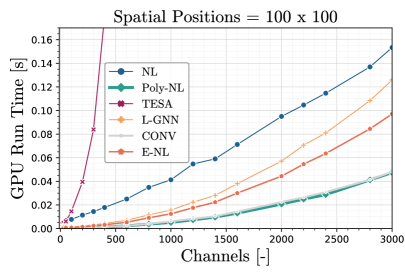
(a)

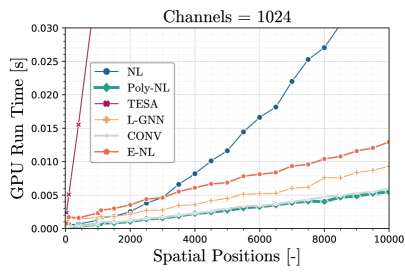
(b)

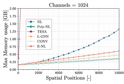
(c)

Figure S3: Runtime and Peak memory consumption performance comparison in vision between Poly-NL, which implements (a variant of) Eq. 9, and other non-local methods executed on a RTX2080 GPU. The network utilizing the Hadamard product exhibits lower computational overhead than competing methods, which is of importance with an increasing number of spatial positions or channels. The figure is reproduced from [33].

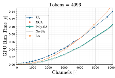
(a)

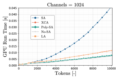
(b)

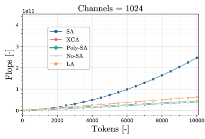
(c)

Figure S4: Runtime and Flops comparison in text domain between Poly-SA, which implements (a variant of) Eq. 9, and two other self-attention method executed on a RTX2080 GPU. The network utilizing the Hadamard product exhibits lower computational overhead than competing methods, with a complexity comparable to a linear layer using no attention mechanism. The figure is reproduced from [33].

S.4 Hadamard product in large language models

In this section, we review the use of the Hadamard product in large language models (LLMs). Related literature is summarized in Table I.

Within the category of adaptive modulation, the Hadamard product appears in LLMs in two main ways. Firstly, it is used in masked language modeling, as discussed in Eq. 7 of the main body. During LLM pre-training, the objective is to predict the next token based on all preceding tokens. A masking mechanism enables this prediction to occur in a single forward pass, while ensuring that a query cannot access keys corresponding to future tokens. An indicative PyTorch implementation is provided in Section S.2.1. Secondly, the Hadamard product functions as a gating mechanism in the core architecture blocks of LLMs, as detailed in Section 4.2. For example, recent models such as xLSTM [8], Mamba [29, 30], and others [31, 32] have adopted the Hadamard product in this role.

Beyond adaptive modulation, the Hadamard product is also employed in parameter-efficient fine-tuning methods for LLMs [35, 36, 37]. Given a pretrained weight matrix $\bm{W}^{0}$, standard LoRA assumes that the fine-tuned weight $\bm{W}^{\star}$ satisfies

$$\bm{W}^{\star}=\bm{W}^{0}+\Delta\bm{W}=\bm{W}^{0}+\bm{A}\bm{B},$$

where $\bm{A}\bm{B}$ represents a low-rank adaptation. A recent method, HIRA [36], modifies this update rule to retain high-rank updates and enhance model capacity:

$$\bm{W}^{\star}=\bm{W}^{0}+\bm{W}^{0}*(\bm{A}\bm{B}).$$

In addition to HIRA, several other LoRA variants incorporating the Hadamard product have also been proposed [35, 37].

References

- [1] J. Hu, L. Shen, and G. Sun, “Squeeze-and-excitation networks,” in Conference on Computer Vision and Pattern Recognition (CVPR), 2018, pp. 7132–7141.
- [2] T. Karras, S. Laine, and T. Aila, “A style-based generator architecture for generative adversarial networks,” in Conference on Computer Vision and Pattern Recognition (CVPR), 2019.
- [3] T. Park, M.-Y. Liu, T.-C. Wang, and J.-Y. Zhu, “Semantic image synthesis with spatially-adaptive normalization,” in Conference on Computer Vision and Pattern Recognition (CVPR), 2019, pp. 2337–2346.
- [4] D. Pathak, P. Krahenbuhl, J. Donahue, T. Darrell, and A. A. Efros, “Context encoders: Feature learning by inpainting,” in Conference on Computer Vision and Pattern Recognition (CVPR), 2016, pp. 2536–2544.
- [5] J. Yu, Z. Lin, J. Yang, X. Shen, X. Lu, and T. S. Huang, “Generative image inpainting with contextual attention,” in Conference on Computer Vision and Pattern Recognition (CVPR), 2018, pp. 5505–5514.
- [6] Y. N. Dauphin, A. Fan, M. Auli, and D. Grangier, “Language modeling with gated convolutional networks,” in International Conference on Machine Learning (ICML), 2017, pp. 933–941.
- [7] J. Devlin, M.-W. Chang, K. Lee, and K. Toutanova, “Bert: Pre-training of deep bidirectional transformers for language understanding,” in Proceedings of the 2019 Conference of the North American Chapter of the Association for Computational Linguistics, 2019.
- [8] S. Hochreiter and J. Schmidhuber, “Long short-term memory,” Neural computation, vol. 9, no. 8, pp. 1735–1780, 1997.
- [9] K. Cho, B. van Merriënboer, D. Bahdanau, and Y. Bengio, “On the properties of neural machine translation: Encoder–decoder approaches,” in Proceedings of SSST-8, Eighth Workshop on Syntax, Semantics and Structure in Statistical Translation, 2014, pp. 103–111.
- [10] A. Vaswani, N. Shazeer, N. Parmar, J. Uszkoreit, L. Jones, A. N. Gomez, Ł. Kaiser, and I. Polosukhin, “Attention is all you need,” in Advances in neural information processing systems (NeurIPS), 2017, pp. 5998–6008.
- [11] S. Antol, A. Agrawal, J. Lu, M. Mitchell, D. Batra, C. L. Zitnick, and D. Parikh, “Vqa: Visual question answering,” in International Conference on Computer Vision (ICCV), 2015, pp. 2425–2433.
- [12] A. Fukui, D. H. Park, D. Yang, A. Rohrbach, T. Darrell, and M. Rohrbach, “Multimodal compact bilinear pooling for visual question answering and visual grounding,” in Empirical Methods in Natural Language Processing (EMNLP), 2016.
- [13] F. D. Keles, P. M. Wijewardena, and C. Hegde, “On the computational complexity of self-attention,” in International Conference on Algorithmic Learning Theory (ALT), 2023.
- [14] F. Babiloni, I. Marras, F. Kokkinos, J. Deng, G. Chrysos, and S. Zafeiriou, “Poly-nl: Linear complexity non-local layers with 3rd order polynomials,” in International Conference on Computer Vision (ICCV), 2021, pp. 10 518–10 528.
- [15] W. Hua, Z. Dai, H. Liu, and Q. Le, “Transformer quality in linear time,” in International Conference on Machine Learning (ICML), 2022, pp. 9099–9117.
- [16] R. Bommasani, D. A. Hudson, E. Adeli, R. Altman, S. Arora, S. von Arx, M. S. Bernstein, J. Bohg, A. Bosselut, E. Brunskill et al., “On the opportunities and risks of foundation models,” arXiv preprint arXiv:2108.07258, 2021.
- [17] S. T. Wasim, M. U. Khattak, M. Naseer, S. Khan, M. Shah, and F. S. Khan, “Video-focalnets: Spatio-temporal focal modulation for video action recognition,” in International Conference on Computer Vision (ICCV), 2023, pp. 13 778–13 789.
- [18] Y. Chen, G. G. Chrysos, M. Georgopoulos, and V. Cevher, “Multilinear operator networks,” in International Conference on Learning Representations (ICLR), 2024.
- [19] D. Fu, S. Arora, J. Grogan, I. Johnson, E. S. Eyuboglu, A. Thomas, B. Spector, M. Poli, A. Rudra, and C. Ré, “Monarch mixer: A simple sub-quadratic gemm-based architecture,” in Advances in neural information processing systems (NeurIPS), vol. 36, 2023.
- [20] Q. Fan, H. Huang, M. Chen, H. Liu, and R. He, “Rmt: Retentive networks meet vision transformers,” in Conference on Computer Vision and Pattern Recognition (CVPR), 2024, pp. 5641–5651.
- [21] B. Zou, C. Yang, Y. Qiao, C. Quan, and Y. Zhao, “Language-aware visual semantic distillation for video question answering,” in Conference on Computer Vision and Pattern Recognition (CVPR), 2024, pp. 27 113–27 123.
- [22] O. Bar-Tal, L. Yariv, Y. Lipman, and T. Dekel, “Multidiffusion: Fusing diffusion paths for controlled image generation,” in International Conference on Machine Learning (ICML), 2023.
- [23] Y. Kim, J. Lee, J.-H. Kim, J.-W. Ha, and J.-Y. Zhu, “Dense text-to-image generation with attention modulation,” in International Conference on Computer Vision (ICCV), 2023, pp. 7701–7711.
- [24] Y. Duan, W. Wang, Z. Chen, X. Zhu, L. Lu, T. Lu, Y. Qiao, H. Li, J. Dai, and W. Wang, “Vision-rwkv: Efficient and scalable visual perception with rwkv-like architectures,” in International Conference on Learning Representations (ICLR), 2025.
- [25] L. Iurada, M. Ciccone, and T. Tommasi, “Finding lottery tickets in vision models via data-driven spectral foresight pruning,” in Conference on Computer Vision and Pattern Recognition (CVPR), 2024, pp. 16 142–16 151.
- [26] T. Cao, K. Kreis, S. Fidler, N. Sharp, and K. Yin, “Texfusion: Synthesizing 3d textures with text-guided image diffusion models,” in International Conference on Computer Vision (ICCV), 2023, pp. 4169–4181.
- [27] J. J. A. Guerreiro, N. Inoue, K. Masui, M. Otani, and H. Nakayama, “Layoutflow: flow matching for layout generation,” in European Conference on Computer Vision (ECCV). Springer, 2024, pp. 56–72.
- [28] S. Yang, B. Wang, Y. Zhang, Y. Shen, and Y. Kim, “Parallelizing linear transformers with the delta rule over sequence length,” in Advances in neural information processing systems (NeurIPS), 2024.
- [29] A. Gu and T. Dao, “Mamba: Linear-time sequence modeling with selective state spaces,” in First Conference on Language Modeling, 2024.
- [30] T. Dao and A. Gu, “Transformers are ssms: Generalized models and efficient algorithms through structured state space duality,” in International Conference on Machine Learning (ICML), 2024.
- [31] Z. Qin, S. Yang, W. Sun, X. Shen, D. Li, W. Sun, and Y. Zhong, “HGRN2: Gated linear RNNs with state expansion,” in First Conference on Language Modeling, 2024.
- [32] S. Yang, B. Wang, Y. Shen, R. Panda, and Y. Kim, “Gated linear attention transformers with hardware-efficient training,” in International Conference on Machine Learning (ICML), 2024.
- [33] F. Babiloni, I. Marras, J. Deng, F. Kokkinos, M. Maggioni, G. Chrysos, P. Torr, and S. Zafeiriou, “Linear complexity self-attention with 3rd order polynomials,” IEEE Transactions on Pattern Analysis and Machine Intelligence (T-PAMI), vol. 45, no. 11, pp. 12 726–12 737, 2023.
- [34] X. Ma, X. Dai, Y. Bai, Y. Wang, and Y. Fu, “Rewrite the stars,” in Conference on Computer Vision and Pattern Recognition (CVPR), 2024, pp. 5694–5703.
- [35] N. Hyeon-Woo, M. Ye-Bin, and T.-H. Oh, “Fedpara: Low-rank hadamard product for communication-efficient federated learning,” in International Conference on Learning Representations (ICLR), 2022.
- [36] Q. Huang, T. Ko, Z. Zhuang, L. Tang, and Y. Zhang, “HiRA: Parameter-efficient hadamard high-rank adaptation for large language models,” in International Conference on Learning Representations (ICLR), 2025.
- [37] J. Wang, G. Yang, W. Chen, H. Yi, X. Wu, and Q. Lao, “Mlae: Masked lora experts for parameter-efficient fine-tuning,” arXiv preprint arXiv:2405.18897, 2024.
- [38] G. G. Chrysos, M. Georgopoulos, and Y. Panagakis, “Conditional generation using polynomial expansions,” in Advances in neural information processing systems (NeurIPS), vol. 34, 2021, pp. 28 390–28 404.
- [39] T. G. Kolda and B. W. Bader, “Tensor decompositions and applications,” SIAM review, vol. 51, no. 3, pp. 455–500, 2009.
- [40] J. Shi, X. Zheng, Y. Li, Q. Zhang, and S. Ying, “Multimodal neuroimaging feature learning with multimodal stacked deep polynomial networks for diagnosis of alzheimer’s disease,” IEEE journal of biomedical and health informatics, vol. 22, no. 1, pp. 173–183, 2017.
- [41] A. Katharopoulos, A. Vyas, N. Pappas, and F. Fleuret, “Transformers are rnns: Fast autoregressive transformers with linear attention,” in International Conference on Machine Learning (ICML). PMLR, 2020, pp. 5156–5165.
- [42] Y. Wu, Z. Zhu, F. Liu, G. G. Chrysos, and V. Cevher, “Extrapolation and spectral bias of neural nets with hadamard product: a polynomial net study,” in Advances in neural information processing systems (NeurIPS), 2022.
- [43] P. R. Halmos, Finite dimensional vector spaces. Princeton University Press, 1948, no. 7.
- [44] G. P. Styan, “Hadamard products and multivariate statistical analysis,” Linear algebra and its applications, vol. 6, pp. 217–240, 1973.
- [45] J. Hadamard, Leçons sur la propagation des ondes et les équations de l’hydrodynamique. A. Hermann, 1903.
- [46] ——, “Resolution d’une question relative aux determinants,” Bull. des sciences math., vol. 2, pp. 240–246, 1893.
- [47] C. R. Johnson, Matrix theory and applications. American Mathematical Soc., 1990, vol. 40.
- [48] J. Schur, “Bemerkungen zur theorie der beschränkten bilinearformen mit unendlich vielen veränderlichen.” 1911.
- [49] K. Han, Y. Wang, H. Chen, X. Chen, J. Guo, Z. Liu, Y. Tang, A. Xiao, C. Xu, Y. Xu et al., “A survey on vision transformer,” IEEE Transactions on Pattern Analysis and Machine Intelligence (T-PAMI), 2022.
- [50] Y. Yu, X. Si, C. Hu, and J. Zhang, “A review of recurrent neural networks: Lstm cells and network architectures,” Neural computation, vol. 31, no. 7, pp. 1235–1270, 2019.
- [51] A. Labach, H. Salehinejad, and S. Valaee, “Survey of dropout methods for deep neural networks,” arXiv preprint arXiv:1904.13310, 2019.
- [52] N. D. Sidiropoulos, L. De Lathauwer, X. Fu, K. Huang, E. E. Papalexakis, and C. Faloutsos, “Tensor decomposition for signal processing and machine learning,” IEEE Transactions on Signal Processing, vol. 65, no. 13, pp. 3551–3582, 2017.
- [53] Y. Panagakis, J. Kossaifi, G. G. Chrysos, J. Oldfield, M. A. Nicolaou, A. Anandkumar, and S. Zafeiriou, “Tensor methods in computer vision and deep learning,” Proceedings of the IEEE, vol. 109, no. 5, pp. 863–890, 2021.
- [54] M. Dalla Mura, S. Prasad, F. Pacifici, P. Gamba, J. Chanussot, and J. A. Benediktsson, “Challenges and opportunities of multimodality and data fusion in remote sensing,” Proceedings of the IEEE, vol. 103, no. 9, pp. 1585–1601, 2015.
- [55] M. H. Stone, “The generalized Weierstrass approximation theorem,” Math. Mag., vol. 21, no. 5, pp. 237–254, 1948.
- [56] S. Nikol’skii, Analysis III: Spaces of Differentiable Functions, ser. Encyclopaedia of Mathematical Sciences. Springer Berlin Heidelberg, 2013.
- [57] A. G. Ivakhnenko, “Polynomial theory of complex systems,” Transactions on Systems, Man, and Cybernetics, no. 4, pp. 364–378, 1971.
- [58] S.-K. Oh, W. Pedrycz, and B.-J. Park, “Polynomial neural networks architecture: analysis and design,” Computers & Electrical Engineering, vol. 29, no. 6, pp. 703–725, 2003.
- [59] G. E. Hinton and T. J. Sejnowski, “Optimal perceptual inference,” in Conference on Computer Vision and Pattern Recognition (CVPR), vol. 448, 1983, pp. 448–453.
- [60] D. Psaltis and C. H. Park, “Nonlinear discriminant functions and associative memories,” in AIP conference Proceedings, vol. 151, no. 1. American Institute of Physics, 1986, pp. 370–375.
- [61] T. J. Sejnowski, “Higher-order boltzmann machines,” in AIP Conference Proceedings, vol. 151, no. 1. American Institute of Physics, 1986, pp. 398–403.
- [62] C. L. Giles and T. Maxwell, “Learning, invariance, and generalization in high-order neural networks,” Applied optics, vol. 26, no. 23, pp. 4972–4978, 1987.
- [63] Y. Shin and J. Ghosh, “The pi-sigma network: An efficient higher-order neural network for pattern classification and function approximation,” in International Joint Conference on Neural Networks (IJCNN), vol. 1, 1991, pp. 13–18.
- [64] R. K. Srivastava, K. Greff, and J. Schmidhuber, “Training very deep networks,” Advances in neural information processing systems (NeurIPS), vol. 28, 2015.
- [65] Y. Wang, L. Xie, C. Liu, S. Qiao, Y. Zhang, W. Zhang, Q. Tian, and A. Yuille, “Sort: Second-order response transform for visual recognition,” in International Conference on Computer Vision (ICCV), 2017, pp. 1359–1368.
- [66] X. Dong, J. Huang, Y. Yang, and S. Yan, “More is less: A more complicated network with less inference complexity,” in Conference on Computer Vision and Pattern Recognition (CVPR), 2017, pp. 5840–5848.
- [67] H. Liu, Z. Dai, D. So, and Q. V. Le, “Pay attention to mlps,” Advances in neural information processing systems (NeurIPS), vol. 34, pp. 9204–9215, 2021.
- [68] Y. Peng, S. Dalmia, I. Lane, and S. Watanabe, “Branchformer: Parallel mlp-attention architectures to capture local and global context for speech recognition and understanding,” in International Conference on Machine Learning (ICML), 2022, pp. 17 627–17 643.
- [69] M. Go and H. Tachibana, “gswin: Gated mlp vision model with hierarchical structure of shifted window,” arXiv preprint arXiv:2208.11718, 2022.
- [70] H. Pan, S. He, K. Zhang, B. Qu, C. Chen, and K. Shi, “Amam: An attention-based multimodal alignment model for medical visual question answering,” Knowledge-Based Systems, vol. 255, p. 109763, 2022.
- [71] M. Wang, X. He, L. Liu, L. Qing, H. Chen, Y. Liu, and C. Ren, “Medical visual question answering based on question-type reasoning and semantic space constraint,” Artificial Intelligence in Medicine, vol. 131, p. 102346, 2022.
- [72] G. G. Chrysos, B. Wang, J. Deng, and V. Cevher, “Regularization of polynomial networks for image recognition,” in Conference on Computer Vision and Pattern Recognition (CVPR), 2023, pp. 16 123–16 132.
- [73] Y. Xu, Q. Kong, W. Wang, and M. D. Plumbley, “Large-scale weakly supervised audio classification using gated convolutional neural network,” in International Conference on Acoustics, Speech and Signal Processing (ICASSP), 2018, pp. 121–125.
- [74] G. G. Chrysos, M. Georgopoulos, J. Deng, J. Kossaifi, Y. Panagakis, and A. Anandkumar, “Augmenting deep classifiers with polynomial neural networks,” in European Conference on Computer Vision (ECCV), 2022, pp. 692–716.
- [75] G. G. Chrysos, S. Moschoglou, G. Bouritsas, Y. Panagakis, J. Deng, and S. Zafeiriou, “nets: Deep polynomial neural networks,” in Conference on Computer Vision and Pattern Recognition (CVPR), 2020, pp. 7325–7335.
- [76] R. Fathony, A. K. Sahu, D. Willmott, and J. Z. Kolter, “Multiplicative filter networks,” in International Conference on Learning Representations (ICLR), 2021.
- [77] D. B. Lindell, D. Van Veen, J. J. Park, and G. Wetzstein, “Bacon: Band-limited coordinate networks for multiscale scene representation,” in Conference on Computer Vision and Pattern Recognition (CVPR), 2022, pp. 16 252–16 262.
- [78] S. Shekarforoush, D. B. Lindell, D. J. Fleet, and M. A. Brubaker, “Residual multiplicative filter networks for multiscale reconstruction,” arXiv preprint arXiv:2206.00746, 2022.
- [79] I. Goodfellow, J. Pouget-Abadie, M. Mirza, B. Xu, D. Warde-Farley, S. Ozair, A. Courville, and Y. Bengio, “Generative adversarial nets,” in Advances in neural information processing systems (NeurIPS), 2014.
- [80] X. Huang and S. Belongie, “Arbitrary style transfer in real-time with adaptive instance normalization,” in International Conference on Computer Vision (ICCV), 2017, pp. 1501–1510.
- [81] W. Nie, T. Karras, A. Garg, S. Debnath, A. Patney, A. Patel, and A. Anandkumar, “Semi-supervised stylegan for disentanglement learning,” in International Conference on Machine Learning (ICML), 2020, pp. 7360–7369.
- [82] G. G. Chrysos, J. Kossaifi, Z. Yu, and A. Anandkumar, “Unsupervised controllable generation with self-training,” in International Joint Conference on Neural Networks (IJCNN), 2021, pp. 1–8.
- [83] J. Hu, L. Shen, S. Albanie, G. Sun, and A. Vedaldi, “Gather-excite: Exploiting feature context in convolutional neural networks,” Advances in neural information processing systems (NeurIPS), vol. 31, 2018.
- [84] S. Woo, J. Park, J.-Y. Lee, and I. S. Kweon, “Cbam: Convolutional block attention module,” in European Conference on Computer Vision (ECCV), 2018, pp. 3–19.
- [85] Z. Qin, P. Zhang, F. Wu, and X. Li, “Fcanet: Frequency channel attention networks,” in International Conference on Computer Vision (ICCV), 2021, pp. 783–792.
- [86] X. Li, W. Wang, X. Hu, and J. Yang, “Selective kernel networks,” in Conference on Computer Vision and Pattern Recognition (CVPR), 2019, pp. 510–519.
- [87] G. Gao, P. You, R. Pan, S. Han, Y. Zhang, Y. Dai, and H. Lee, “Neural image compression via attentional multi-scale back projection and frequency decomposition,” in International Conference on Computer Vision (ICCV), 2021, pp. 14 677–14 686.
- [88] Y. Zhang, K. Li, K. Li, L. Wang, B. Zhong, and Y. Fu, “Image super-resolution using very deep residual channel attention networks,” in European Conference on Computer Vision (ECCV), 2018, pp. 286–301.
- [89] S. Anwar and N. Barnes, “Real image denoising with feature attention,” in International Conference on Computer Vision (ICCV), 2019, pp. 3155–3164.
- [90] H. Zhang, K. Dana, J. Shi, Z. Zhang, X. Wang, A. Tyagi, and A. Agrawal, “Context encoding for semantic segmentation,” in Conference on Computer Vision and Pattern Recognition (CVPR), 2018, pp. 7151–7160.
- [91] Z.-L. Ni, G.-B. Bian, Z. Li, X.-H. Zhou, R.-Q. Li, and Z.-G. Hou, “Space squeeze reasoning and low-rank bilinear feature fusion for surgical image segmentation,” IEEE Journal of Biomedical and Health Informatics, 2022.
- [92] J. Wang, S. Tian, L. Yu, Y. Wang, F. Wang, and Z. Zhou, “Sbdf-net: A versatile dual-branch fusion network for medical image segmentation,” Biomedical Signal Processing and Control, vol. 78, p. 103928, 2022.
- [93] Z.-L. Ni, X.-H. Zhou, G.-A. Wang, W.-Q. Yue, Z. Li, G.-B. Bian, and Z.-G. Hou, “Surginet: Pyramid attention aggregation and class-wise self-distillation for surgical instrument segmentation,” Medical Image Analysis, vol. 76, p. 102310, 2022.
- [94] L. Pan, X. Chen, Z. Cai, J. Zhang, H. Zhao, S. Yi, and Z. Liu, “Variational relational point completion network,” in Conference on Computer Vision and Pattern Recognition (CVPR), 2021, pp. 8524–8533.
- [95] H. Tang, X. Qi, D. Xu, P. H. Torr, and N. Sebe, “Edge guided gans with semantic preserving for semantic image synthesis,” arXiv preprint arXiv:2003.13898, 2020.
- [96] J. Cheng, S. Tian, L. Yu, H. Lu, and X. Lv, “Fully convolutional attention network for biomedical image segmentation,” Artificial Intelligence in Medicine, vol. 107, p. 101899, 2020.
- [97] Z.-L. Ni, G.-B. Bian, G.-A. Wang, X.-H. Zhou, Z.-G. Hou, H.-B. Chen, and X.-L. Xie, “Pyramid attention aggregation network for semantic segmentation of surgical instruments,” in AAAI Conference on Artificial Intelligence, vol. 34, no. 07, 2020, pp. 11 782–11 790.
- [98] C. Xiong, S. Merity, and R. Socher, “Dynamic memory networks for visual and textual question answering,” in International Conference on Machine Learning (ICML), 2016, pp. 2397–2406.
- [99] J. Chen, H. Hu, H. Wu, Y. Jiang, and C. Wang, “Learning the best pooling strategy for visual semantic embedding,” in Conference on Computer Vision and Pattern Recognition (CVPR), 2021, pp. 15 789–15 798.
- [100] X. Wu, Y. Lao, L. Jiang, X. Liu, and H. Zhao, “Point transformer v2: Grouped vector attention and partition-based pooling,” in Advances in neural information processing systems (NeurIPS), 2022.
- [101] S. Ploumpis, S. Moschoglou, V. Triantafyllou, and S. Zafeiriou, “3d human tongue reconstruction from single ”in-the-wild” images,” in Conference on Computer Vision and Pattern Recognition (CVPR), 2022, pp. 2771–2780.
- [102] G. G. Chrysos, S. Moschoglou, G. Bouritsas, J. Deng, Y. Panagakis, and S. Zafeiriou, “Deep polynomial neural networks,” IEEE Transactions on Pattern Analysis and Machine Intelligence (T-PAMI), vol. 44, no. 8, pp. 4021–4034, 2021.
- [103] X. Chu, W. Yang, W. Ouyang, C. Ma, A. L. Yuille, and X. Wang, “Multi-context attention for human pose estimation,” in Conference on Computer Vision and Pattern Recognition (CVPR), 2017, pp. 1831–1840.
- [104] Y. Wu, G. G. Chrysos, and V. Cevher, “Adversarial audio synthesis with complex-valued polynomial networks,” arXiv preprint arXiv:2206.06811, 2022.
- [105] J. Yang, C. Li, and J. Gao, “Focal modulation networks,” in Advances in neural information processing systems (NeurIPS), 2022.
- [106] A. Wu, L. Zhu, Y. Han, and Y. Yang, “Connective cognition network for directional visual commonsense reasoning,” Advances in neural information processing systems (NeurIPS), vol. 32, 2019.
- [107] S. Ging, M. Zolfaghari, H. Pirsiavash, and T. Brox, “Coot: Cooperative hierarchical transformer for video-text representation learning,” Advances in neural information processing systems (NeurIPS), vol. 33, pp. 22 605–22 618, 2020.
- [108] J. Gao and C. Xu, “Fast video moment retrieval,” in International Conference on Computer Vision (ICCV), 2021, pp. 1523–1532.
- [109] H. Pan and J. Huang, “Multimodal high-order relational network for vision-and-language tasks,” Neurocomputing, vol. 492, pp. 62–75, 2022.
- [110] D. Lahat, T. Adali, and C. Jutten, “Multimodal data fusion: an overview of methods, challenges, and prospects,” Proceedings of the IEEE, vol. 103, no. 9, pp. 1449–1477, 2015.
- [111] H. Harold, “Relations between two sets of variates,” Biometrika, vol. 28, no. 3/4, p. 321, 1936.
- [112] R. B. Cattell, ““parallel proportional profiles” and other principles for determining the choice of factors by rotation,” Psychometrika, vol. 9, no. 4, pp. 267–283, 1944.
- [113] B. Vinograde, “Canonical positive definite matrices under internal linear transformations,” Proceedings of the American Mathematical Society, vol. 1, no. 2, pp. 159–161, 1950.
- [114] J. R. Kettenring, “Canonical analysis of several sets of variables,” Biometrika, vol. 58, no. 3, pp. 433–451, 1971.
- [115] J. D. Carroll and J.-J. Chang, “Analysis of individual differences in multidimensional scaling via an n-way generalization of “Eckart-Young” decomposition,” Psychometrika, vol. 35, pp. 283–319, 1970.
- [116] E. D. Petajan, “Automatic lipreading to enhance speech recognition (speech reading),” Ph.D. dissertation, 1984.
- [117] W. H. Sumby and I. Pollack, “Visual contribution to speech intelligibility in noise,” The journal of the acoustical society of america, vol. 26, no. 2, pp. 212–215, 1954.
- [118] H. McGurk and J. MacDonald, “Hearing lips and seeing voices,” Nature, vol. 264, no. 5588, pp. 746–748, 1976.
- [119] B. P. Yuhas, M. H. Goldstein, and T. J. Sejnowski, “Integration of acoustic and visual speech signals using neural networks,” Communications Magazine, vol. 27, no. 11, pp. 65–71, 1989.
- [120] D. Teney, P. Anderson, X. He, and A. Van Den Hengel, “Tips and tricks for visual question answering: Learnings from the 2017 challenge,” in Conference on Computer Vision and Pattern Recognition (CVPR), 2018, pp. 4223–4232.
- [121] J.-H. Kim, S.-W. Lee, D. Kwak, M.-O. Heo, J. Kim, J.-W. Ha, and B.-T. Zhang, “Multimodal residual learning for visual qa,” in Advances in neural information processing systems (NeurIPS), vol. 29, 2016.
- [122] H. Ben-Younes, R. Cadene, M. Cord, and N. Thome, “Mutan: Multimodal tucker fusion for visual question answering,” in International Conference on Computer Vision (ICCV), 2017, pp. 2612–2620.
- [123] Z. Sun, Z.-H. Deng, J.-Y. Nie, and J. Tang, “Rotate: Knowledge graph embedding by relational rotation in complex space,” in International Conference on Learning Representations (ICLR), 2019.
- [124] Y. Chen, S. Gong, and L. Bazzani, “Image search with text feedback by visiolinguistic attention learning,” in Conference on Computer Vision and Pattern Recognition (CVPR), 2020, pp. 3001–3011.
- [125] S. Chen, Y. Zhao, Q. Jin, and Q. Wu, “Fine-grained video-text retrieval with hierarchical graph reasoning,” in Conference on Computer Vision and Pattern Recognition (CVPR), 2020, pp. 10 638–10 647.
- [126] Y. Hong, C. Rodriguez, Y. Qi, Q. Wu, and S. Gould, “Language and visual entity relationship graph for agent navigation,” in Advances in neural information processing systems (NeurIPS), vol. 33, 2020, pp. 7685–7696.
- [127] B. Li, X. Qi, T. Lukasiewicz, and P. Torr, “Controllable text-to-image generation,” Advances in neural information processing systems (NeurIPS), vol. 32, 2019.
- [128] P. Anderson, X. He, C. Buehler, D. Teney, M. Johnson, S. Gould, and L. Zhang, “Bottom-up and top-down attention for image captioning and visual question answering,” in Conference on Computer Vision and Pattern Recognition (CVPR), 2018, pp. 6077–6086.
- [129] J. Lu, D. Batra, D. Parikh, and S. Lee, “Vilbert: Pretraining task-agnostic visiolinguistic representations for vision-and-language tasks,” in Advances in neural information processing systems (NeurIPS), vol. 32, 2019.
- [130] J. Lu, V. Goswami, M. Rohrbach, D. Parikh, and S. Lee, “12-in-1: Multi-task vision and language representation learning,” in Conference on Computer Vision and Pattern Recognition (CVPR), 2020, pp. 10 437–10 446.
- [131] L. Zhou, H. Palangi, L. Zhang, H. Hu, J. Corso, and J. Gao, “Unified vision-language pre-training for image captioning and vqa,” in AAAI Conference on Artificial Intelligence, vol. 34, no. 07, 2020, pp. 13 041–13 049.
- [132] Q. CAO, P. KHANNA, N. D. LANE, and A. BALASUBRAMANIAN, “Mobivqa: Efficient on-device visual question answering,” Proc. ACM Interact. Mob. Wearable Ubiquitous Technol., vol. 6, no. 2, jul 2022.
- [133] B. X. Nguyen, T. Do, H. Tran, E. Tjiputra, Q. D. Tran, and A. Nguyen, “Coarse-to-fine reasoning for visual question answering,” in Conference on Computer Vision and Pattern Recognition (CVPR), 2022, pp. 4558–4566.
- [134] Y. Xiang, C. Zhang, Z. Han, H. Yu, J. Li, and L. Zhu, “Path-wise attention memory network for visual question answering,” Mathematics, vol. 10, no. 18, p. 3244, 2022.
- [135] D. Gao, R. Wang, Z. Bai, and X. Chen, “Env-qa: A video question answering benchmark for comprehensive understanding of dynamic environments,” in International Conference on Computer Vision (ICCV), 2021, pp. 1675–1685.
- [136] H. Zhang, Z. Kyaw, J. Yu, and S.-F. Chang, “Ppr-fcn: Weakly supervised visual relation detection via parallel pairwise r-fcn,” in International Conference on Computer Vision (ICCV), 2017, pp. 4233–4241.
- [137] J. M. Ramirez and H. Arguello, “Spectral image classification from multi-sensor compressive measurements,” IEEE Transactions on Geoscience and Remote Sensing, vol. 58, no. 1, pp. 626–636, 2019.
- [138] M. Georgopoulos, G. Chrysos, M. Pantic, and Y. Panagakis, “Multilinear latent conditioning for generating unseen attribute combinations,” International Conference on Machine Learning (ICML), 2020.
- [139] L. Li and H. Ma, “Saliency-guided nonsubsampled shearlet transform for multisource remote sensing image fusion,” Sensors, vol. 21, no. 5, p. 1756, 2021.
- [140] J. M. Ramirez, J. I. Martínez-Torre, and H. Arguello, “Ladmm-net: An unrolled deep network for spectral image fusion from compressive data,” Signal Processing, vol. 189, p. 108239, 2021.
- [141] S. K. Kumaraswamy, M. Shi, and E. Kijak, “Detecting human-object interaction with mixed supervision,” in Winter Conference on Applications of Computer Vision (WACV), 2021, pp. 1228–1237.
- [142] J. Lu, C. Shan, K. Jin, X. Deng, S. Wang, Y. Wu, J. Li, and Y. Guo, “Onavi: Data-driven based multi-sensor fusion positioning system in indoor environments,” in 2022 IEEE 12th International Conference on Indoor Positioning and Indoor Navigation (IPIN), 2022, pp. 1–8.
- [143] T. Durand, “Learning user representations for open vocabulary image hashtag prediction,” in Conference on Computer Vision and Pattern Recognition (CVPR), 2020, pp. 9769–9778.
- [144] H. De Vries, F. Strub, J. Mary, H. Larochelle, O. Pietquin, and A. C. Courville, “Modulating early visual processing by language,” in Advances in neural information processing systems (NeurIPS), 2017, pp. 6594–6604.
- [145] H. Nam, J.-W. Ha, and J. Kim, “Dual attention networks for multimodal reasoning and matching,” in Conference on Computer Vision and Pattern Recognition (CVPR), 2017, pp. 299–307.
- [146] T. Chen, M. Lucic, N. Houlsby, and S. Gelly, “On self modulation for generative adversarial networks,” in International Conference on Learning Representations (ICLR), 2019.
- [147] L. Zhou, Y. Zhou, J. J. Corso, R. Socher, and C. Xiong, “End-to-end dense video captioning with masked transformer,” in Conference on Computer Vision and Pattern Recognition (CVPR), 2018, pp. 8739–8748.
- [148] Z. Yu, J. Yu, C. Xiang, J. Fan, and D. Tao, “Beyond bilinear: Generalized multimodal factorized high-order pooling for visual question answering,” IEEE Transactions on Neural Networks and Learning Systems (T-NN), vol. 29, no. 12, pp. 5947–5959, 2018.
- [149] C. Deng, Q. Wu, Q. Wu, F. Hu, F. Lyu, and M. Tan, “Visual grounding via accumulated attention,” in Conference on Computer Vision and Pattern Recognition (CVPR), 2018, pp. 7746–7755.
- [150] B. Duke and G. W. Taylor, “Generalized hadamard-product fusion operators for visual question answering,” in 2018 15th Conference on Computer and Robot Vision (CRV). IEEE, 2018, pp. 39–46.
- [151] P. Gao, H. You, Z. Zhang, X. Wang, and H. Li, “Multi-modality latent interaction network for visual question answering,” in International Conference on Computer Vision (ICCV), 2019, pp. 5825–5835.
- [152] C.-H. Lee, Z. Liu, L. Wu, and P. Luo, “Maskgan: Towards diverse and interactive facial image manipulation,” in Conference on Computer Vision and Pattern Recognition (CVPR), 2020, pp. 5549–5558.
- [153] H. Jiang, I. Misra, M. Rohrbach, E. Learned-Miller, and X. Chen, “In defense of grid features for visual question answering,” in Conference on Computer Vision and Pattern Recognition (CVPR), 2020, pp. 10 267–10 276.
- [154] E.-S. Kim, W. Y. Kang, K.-W. On, Y.-J. Heo, and B.-T. Zhang, “Hypergraph attention networks for multimodal learning,” in Conference on Computer Vision and Pattern Recognition (CVPR), 2020, pp. 14 581–14 590.
- [155] Q. Xia, C. Yu, P. Peng, H. Gu, Z. Zheng, and K. Zhao, “Visual question answering based on position alignment,” in 2021 14th International Congress on Image and Signal Processing, BioMedical Engineering and Informatics (CISP-BMEI). IEEE, 2021, pp. 1–5.
- [156] A. Akula, V. Jampani, S. Changpinyo, and S.-C. Zhu, “Robust visual reasoning via language guided neural module networks,” Advances in neural information processing systems (NeurIPS), vol. 34, pp. 11 041–11 053, 2021.
- [157] Z. Wang, K. Wang, M. Yu, J. Xiong, W.-m. Hwu, M. Hasegawa-Johnson, and H. Shi, “Interpretable visual reasoning via induced symbolic space,” in International Conference on Computer Vision (ICCV), 2021, pp. 1878–1887.
- [158] F. Zhan, Y. Yu, R. Wu, J. Zhang, K. Cui, A. Xiao, S. Lu, and C. Miao, “Bi-level feature alignment for versatile image translation and manipulation,” in European Conference on Computer Vision (ECCV), 2022, pp. 224–241.
- [159] T. Qiao, J. Zhang, D. Xu, and D. Tao, “Mirrorgan: Learning text-to-image generation by redescription,” in Conference on Computer Vision and Pattern Recognition (CVPR), 2019, pp. 1505–1514.
- [160] W. Liao, K. Hu, M. Y. Yang, and B. Rosenhahn, “Text to image generation with semantic-spatial aware gan,” in Conference on Computer Vision and Pattern Recognition (CVPR), 2022, pp. 18 187–18 196.
- [161] B. Li, X. Qi, T. Lukasiewicz, and P. H. Torr, “Manigan: Text-guided image manipulation,” in Conference on Computer Vision and Pattern Recognition (CVPR), 2020, pp. 7880–7889.
- [162] F. Wu, L. Liu, F. Hao, F. He, and J. Cheng, “Text-to-image synthesis based on object-guided joint-decoding transformer,” in Conference on Computer Vision and Pattern Recognition (CVPR), 2022, pp. 18 113–18 122.
- [163] ——, “Language-based image manipulation built on language-guided ranking,” IEEE Transactions on Multimedia, 2022.
- [164] W. Sun and T. Wu, “Image synthesis from reconfigurable layout and style,” in International Conference on Computer Vision (ICCV), 2019, pp. 10 531–10 540.
- [165] R. Li and J. Jia, “Visual question answering with question representation update (qru),” in Advances in neural information processing systems (NeurIPS), vol. 29, 2016.
- [166] Z. Lv, X. Li, Z. Niu, B. Cao, and W. Zuo, “Semantic-shape adaptive feature modulation for semantic image synthesis,” in Conference on Computer Vision and Pattern Recognition (CVPR), 2022, pp. 11 214–11 223.
- [167] P. Zhu, R. Abdal, Y. Qin, and P. Wonka, “Sean: Image synthesis with semantic region-adaptive normalization,” in Conference on Computer Vision and Pattern Recognition (CVPR), 2020, pp. 5104–5113.
- [168] H. Zhang, J. Y. Koh, J. Baldridge, H. Lee, and Y. Yang, “Cross-modal contrastive learning for text-to-image generation,” in Conference on Computer Vision and Pattern Recognition (CVPR), 2021, pp. 833–842.
- [169] T. Do, T.-T. Do, H. Tran, E. Tjiputra, and Q. D. Tran, “Compact trilinear interaction for visual question answering,” in International Conference on Computer Vision (ICCV), 2019, pp. 392–401.
- [170] X. Xu, J. Sun, Z. Cao, Y. Zhang, X. Zhu, and H. T. Shen, “Tfun: Trilinear fusion network for ternary image-text retrieval,” Information Fusion, vol. 91, pp. 327–337, 2023.
- [171] N. Ruwa, Q. Mao, H. Song, H. Jia, and M. Dong, “Triple attention network for sentimental visual question answering,” Computer Vision and Image Understanding, vol. 189, p. 102829, 2019.
- [172] C. Ma, C. Shen, A. Dick, Q. Wu, P. Wang, A. van den Hengel, and I. Reid, “Visual question answering with memory-augmented networks,” in Conference on Computer Vision and Pattern Recognition (CVPR), 2018, pp. 6975–6984.
- [173] W. Jiang and H. Hu, “Hadamard product perceptron attention for image captioning,” Neural Processing Letters, pp. 1–18, 2022.
- [174] X. Yang, C. Gao, H. Zhang, and J. Cai, “Auto-parsing network for image captioning and visual question answering,” in International Conference on Computer Vision (ICCV), 2021, pp. 2197–2207.
- [175] Y. Liang, P. Zhang, Y. Mei, and T. Wang, “Pmacnet: Parallel multiscale attention constraint network for pan-sharpening,” IEEE Geoscience and Remote Sensing Letters, vol. 19, pp. 1–5, 2022.
- [176] P. Gao, Z. Jiang, H. You, P. Lu, S. C. Hoi, X. Wang, and H. Li, “Dynamic fusion with intra-and inter-modality attention flow for visual question answering,” in Conference on Computer Vision and Pattern Recognition (CVPR), 2019, pp. 6639–6648.
- [177] A.-A. Liu, Y. Zhai, N. Xu, W. Nie, W. Li, and Y. Zhang, “Region-aware image captioning via interaction learning,” IEEE Transactions on Circuits and Systems for Video Technology, 2021.
- [178] R. Hu, A. Rohrbach, T. Darrell, and K. Saenko, “Language-conditioned graph networks for relational reasoning,” in International Conference on Computer Vision (ICCV), 2019, pp. 10 294–10 303.
- [179] C. Jing, Y. Jia, Y. Wu, X. Liu, and Q. Wu, “Maintaining reasoning consistency in compositional visual question answering,” in Conference on Computer Vision and Pattern Recognition (CVPR), 2022, pp. 5099–5108.
- [180] D. Gao, K. Li, R. Wang, S. Shan, and X. Chen, “Multi-modal graph neural network for joint reasoning on vision and scene text,” in Conference on Computer Vision and Pattern Recognition (CVPR), 2020, pp. 12 746–12 756.
- [181] C. Rodriguez-Opazo, E. Marrese-Taylor, B. Fernando, H. Li, and S. Gould, “Dori: discovering object relationships for moment localization of a natural language query in a video,” in Winter Conference on Applications of Computer Vision (WACV), 2021, pp. 1079–1088.
- [182] T. Le, N. Le, and B. Le, “Knowledge graph embedding by relational rotation and complex convolution for link prediction,” Expert Systems with Applications, vol. 214, p. 119122, 2023.
- [183] Z. Zhang, J. Cai, Y. Zhang, and J. Wang, “Learning hierarchy-aware knowledge graph embeddings for link prediction,” in AAAI Conference on Artificial Intelligence, vol. 34, no. 03, 2020, pp. 3065–3072.
- [184] C. Bai and P. Wu, “Prrl: Path rotation based knowledge graph representation learning method,” in 2021 IEEE/ACM 8th International Conference on Big Data Computing, Applications and Technologies (BDCAT’21), 2021, pp. 38–45.
- [185] S. Zhang, Y. Tay, L. Yao, and Q. Liu, “Quaternion knowledge graph embeddings,” Advances in neural information processing systems (NeurIPS), vol. 32, 2019.
- [186] S. M. Kazemi and D. Poole, “Simple embedding for link prediction in knowledge graphs,” Advances in neural information processing systems (NeurIPS), vol. 31, 2018.
- [187] W. Zhang, B. Paudel, W. Zhang, A. Bernstein, and H. Chen, “Interaction embeddings for prediction and explanation in knowledge graphs,” in Proceedings of the Twelfth ACM International Conference on Web Search and Data Mining, 2019, pp. 96–104.
- [188] A. Croitor-Sava, M. Martinez-Bisbal, T. Laudadio, J. Piquer, B. Celda, A. Heerschap, D. Sima, and S. Van Huffel, “Fusing in vivo and ex vivo nmr sources of information for brain tumor classification,” Measurement Science and Technology, vol. 22, no. 11, p. 114012, 2011.
- [189] O. El Mansouri, A. Basarab, M. A. Figueiredo, D. Kouamé, and J.-Y. Tourneret, “Ultrasound and magnetic resonance image fusion using a patch-wise polynomial model,” in International Conference on Image Processing (ICIP), 2020, pp. 403–407.
- [190] X.-C. Lou and X. Feng, “Multimodal medical image fusion based on multiple latent low-rank representation,” Computational and Mathematical Methods in Medicine, vol. 2021, 2021.
- [191] S. A. Hasan, Y. Ling, O. Farri, J. Liu, H. Müller, and M. Lungren, “Overview of imageclef 2018 medical domain visual question answering task,” 10-14 September 2018, Tech. Rep., 2018.
- [192] L.-M. Zhan, B. Liu, L. Fan, J. Chen, and X.-M. Wu, “Medical visual question answering via conditional reasoning,” in Proceedings of the 28th ACM International Conference on Multimedia, 2020, pp. 2345–2354.
- [193] Y. Li, S. Long, Z. Yang, H. Weng, K. Zeng, Z. Huang, F. L. Wang, and T. Hao, “A bi-level representation learning model for medical visual question answering,” Journal of Biomedical Informatics, vol. 134, p. 104183, 2022.
- [194] F. Zhou, R. Hang, and Q. Liu, “Class-guided feature decoupling network for airborne image segmentation,” IEEE Transactions on Geoscience and Remote Sensing, vol. 59, no. 3, pp. 2245–2255, 2020.
- [195] J. Jin, W. Zhou, L. Ye, J. Lei, L. Yu, X. Qian, and T. Luo, “Dasfnet: Dense-attention–similarity-fusion network for scene classification of dual-modal remote-sensing images,” International Journal of Applied Earth Observation and Geoinformation, vol. 115, p. 103087, 2022.
- [196] R. Liu, L. Mi, and Z. Chen, “Afnet: Adaptive fusion network for remote sensing image semantic segmentation,” IEEE Transactions on Geoscience and Remote Sensing, vol. 59, no. 9, pp. 7871–7886, 2020.
- [197] Y. Feng, H. Xu, J. Jiang, H. Liu, and J. Zheng, “Icif-net: Intra-scale cross-interaction and inter-scale feature fusion network for bitemporal remote sensing images change detection,” IEEE Transactions on Geoscience and Remote Sensing, vol. 60, pp. 1–13, 2022.
- [198] X. Zheng, X. Wu, L. Huan, W. He, and H. Zhang, “A gather-to-guide network for remote sensing semantic segmentation of rgb and auxiliary image,” IEEE Transactions on Geoscience and Remote Sensing, vol. 60, pp. 1–15, 2021.
- [199] L. Wan, M. Zeiler, S. Zhang, Y. Le Cun, and R. Fergus, “Regularization of neural networks using dropconnect,” in International Conference on Machine Learning (ICML), 2013, pp. 1058–1066.
- [200] N. Srivastava, G. Hinton, A. Krizhevsky, I. Sutskever, and R. Salakhutdinov, “Dropout: a simple way to prevent neural networks from overfitting,” Journal of Machine Learning Research, vol. 15, no. 1, pp. 1929–1958, 2014.
- [201] H. Liu, D. Tam, M. Muqeeth, J. Mohta, T. Huang, M. Bansal, and C. Raffel, “Few-shot parameter-efficient fine-tuning is better and cheaper than in-context learning,” in Advances in neural information processing systems (NeurIPS), 2022.
- [202] Y. Ren, X. Yu, R. Zhang, T. H. Li, S. Liu, and G. Li, “Structureflow: Image inpainting via structure-aware appearance flow,” in International Conference on Computer Vision (ICCV), 2019, pp. 181–190.
- [203] Z. Yi, Q. Tang, S. Azizi, D. Jang, and Z. Xu, “Contextual residual aggregation for ultra high-resolution image inpainting,” in Conference on Computer Vision and Pattern Recognition (CVPR), 2020, pp. 7508–7517.
- [204] J. Jam, C. Kendrick, V. Drouard, K. Walker, G.-S. Hsu, and M. H. Yap, “R-mnet: A perceptual adversarial network for image inpainting,” in Winter Conference on Applications of Computer Vision (WACV), 2021, pp. 2714–2723.
- [205] G. Wadhwa, A. Dhall, S. Murala, and U. Tariq, “Hyperrealistic image inpainting with hypergraphs,” in Winter Conference on Applications of Computer Vision (WACV), 2021, pp. 3912–3921.
- [206] D. Kim, S. Woo, J.-Y. Lee, and I. S. Kweon, “Deep video inpainting,” in Conference on Computer Vision and Pattern Recognition (CVPR), 2019, pp. 5792–5801.
- [207] A. Atapour-Abarghouei and T. P. Breckon, “Veritatem dies aperit-temporally consistent depth prediction enabled by a multi-task geometric and semantic scene understanding approach,” in Conference on Computer Vision and Pattern Recognition (CVPR), 2019, pp. 3373–3384.
- [208] L. Hoyer, D. Dai, Y. Chen, A. Koring, S. Saha, and L. Van Gool, “Three ways to improve semantic segmentation with self-supervised depth estimation,” in Conference on Computer Vision and Pattern Recognition (CVPR), 2021, pp. 11 130–11 140.
- [209] D. Pavllo, G. Spinks, T. Hofmann, M.-F. Moens, and A. Lucchi, “Convolutional generation of textured 3d meshes,” in Advances in neural information processing systems (NeurIPS), vol. 33, 2020, pp. 870–882.
- [210] R. Abdal, Y. Qin, and P. Wonka, “Image2stylegan++: How to edit the embedded images?” in Conference on Computer Vision and Pattern Recognition (CVPR), 2020, pp. 8296–8305.
- [211] H. Tang, D. Xu, Y. Yan, P. H. Torr, and N. Sebe, “Local class-specific and global image-level generative adversarial networks for semantic-guided scene generation,” in Conference on Computer Vision and Pattern Recognition (CVPR), 2020, pp. 7870–7879.
- [212] T. Hui, S. Liu, S. Huang, G. Li, S. Yu, F. Zhang, and J. Han, “Linguistic structure guided context modeling for referring image segmentation,” in European Conference on Computer Vision (ECCV), 2020, pp. 59–75.
- [213] G. Liu, F. A. Reda, K. J. Shih, T.-C. Wang, A. Tao, and B. Catanzaro, “Image inpainting for irregular holes using partial convolutions,” in European Conference on Computer Vision (ECCV), 2018, pp. 85–100.
- [214] S. W. Oh, S. Lee, J.-Y. Lee, and S. J. Kim, “Onion-peel networks for deep video completion,” in International Conference on Computer Vision (ICCV), 2019, pp. 4403–4412.
- [215] J. Frankle and M. Carbin, “The lottery ticket hypothesis: Finding sparse, trainable neural networks,” in International Conference on Learning Representations (ICLR), 2019.
- [216] A. Nova, H. Dai, and D. Schuurmans, “Gradient-free structured pruning with unlabeled data,” in International Conference on Machine Learning (ICML). PMLR, 2023, pp. 26 326–26 341.
- [217] G. E. Hinton, N. Srivastava, A. Krizhevsky, I. Sutskever, and R. R. Salakhutdinov, “Improving neural networks by preventing co-adaptation of feature detectors,” arXiv preprint arXiv:1207.0580, 2012.
- [218] J. Ba and B. Frey, “Adaptive dropout for training deep neural networks,” Advances in neural information processing systems (NeurIPS), vol. 26, 2013.
- [219] L. Wu, J. Li, Y. Wang, Q. Meng, T. Qin, W. Chen, M. Zhang, T.-Y. Liu et al., “R-drop: Regularized dropout for neural networks,” Advances in neural information processing systems (NeurIPS), vol. 34, pp. 10 890–10 905, 2021.
- [220] R. Arora, P. Bartlett, P. Mianjy, and N. Srebro, “Dropout: Explicit forms and capacity control,” in International Conference on Machine Learning (ICML), 2021, pp. 351–361.
- [221] S. Guo, Y. Lin, N. Feng, C. Song, and H. Wan, “Attention based spatial-temporal graph convolutional networks for traffic flow forecasting,” in AAAI Conference on Artificial Intelligence, vol. 33, no. 01, 2019, pp. 922–929.
- [222] H.-Y. Tseng, H.-Y. Lee, J.-B. Huang, and M.-H. Yang, “Cross-domain few-shot classification via learned feature-wise transformation,” in International Conference on Learning Representations (ICLR), 2020.
- [223] A. Radford, K. Narasimhan, T. Salimans, I. Sutskever et al., “Improving language understanding by generative pre-training,” 2018.
- [224] H. Touvron, L. Martin, K. R. Stone, P. Albert, A. Almahairi, and et al., “Llama 2: Open foundation and fine-tuned chat models,” arXiv preprint arXiv:2307.09288, 2023.
- [225] Y. Sun, L. Dong, S. Huang, S. Ma, Y. Xia, J. Xue, J. Wang, and F. Wei, “Retentive network: A successor to transformer for large language models,” arXiv preprint arXiv:2307.08621, 2023.
- [226] M. Beck, K. Pöppel, M. Spanring, A. Auer, O. Prudnikova, M. Kopp, G. Klambauer, J. Brandstetter, and S. Hochreiter, “xlstm: Extended long short-term memory,” in Advances in neural information processing systems (NeurIPS), 2024.
- [227] Y. Zhang, S. Yang, R. Zhu, Y. Zhang, L. Cui, Y. Wang, B. Wang, F. Shi, B. Wang, W. Bi et al., “Gated slot attention for efficient linear-time sequence modeling,” in Advances in neural information processing systems (NeurIPS), 2024.
- [228] J. Bae, M. Kwon, and Y. Uh, “Furrygan: High quality foreground-aware image synthesis,” in European Conference on Computer Vision (ECCV), 2022, pp. 696–712.
- [229] J. Huang, Y. Jin, K. M. Yi, and L. Sigal, “Layered controllable video generation,” in European Conference on Computer Vision (ECCV), 2022, pp. 546–564.
- [230] J. T. Jewell, V. R. Khazaie, and Y. Mohsenzadeh, “One-class learned encoder-decoder network with adversarial context masking for novelty detection,” in Winter Conference on Applications of Computer Vision (WACV), 2022, pp. 3591–3601.
- [231] C. Xie, S. Liu, C. Li, M.-M. Cheng, W. Zuo, X. Liu, S. Wen, and E. Ding, “Image inpainting with learnable bidirectional attention maps,” in International Conference on Computer Vision (ICCV), 2019, pp. 8858–8867.
- [232] F. Cong, S. Xu, L. Guo, and Y. Tian, “Anomaly matters: An anomaly-oriented model for medical visual question answering,” IEEE Transactions on Medical Imaging, vol. 41, no. 11, pp. 3385–3397, 2022.
- [233] D. Zhao, Y. Zeng, and Y. Li, “Backeisnn: A deep spiking neural network with adaptive self-feedback and balanced excitatory–inhibitory neurons,” Neural Networks, vol. 154, pp. 68–77, 2022.
- [234] G. Carneiro, T. Peng, C. Bayer, and N. Navab, “Weakly-supervised structured output learning with flexible and latent graphs using high-order loss functions,” in International Conference on Computer Vision (ICCV), 2015, pp. 648–656.
- [235] X. Chen, J. H. Liew, W. Xiong, C.-K. Chui, and S.-H. Ong, “Focus, segment and erase: an efficient network for multi-label brain tumor segmentation,” in European Conference on Computer Vision (ECCV), 2018, pp. 654–669.
- [236] X. Hou, L. Shen, O. Patashnik, D. Cohen-Or, and H. Huang, “Feat: Face editing with attention,” arXiv preprint arXiv:2202.02713, 2022.
- [237] J. Yu, Z. Lin, J. Yang, X. Shen, X. Lu, and T. S. Huang, “Free-form image inpainting with gated convolution,” in International Conference on Computer Vision (ICCV), 2019, pp. 4471–4480.
- [238] X. Liu, G. Yin, J. Shao, X. Wang et al., “Learning to predict layout-to-image conditional convolutions for semantic image synthesis,” Advances in neural information processing systems (NeurIPS), vol. 32, 2019.
- [239] S. N. Rai, R. Saluja, C. Arora, V. N. Balasubramanian, A. Subramanian, and C. Jawahar, “Fluid: Few-shot self-supervised image deraining,” in Winter Conference on Applications of Computer Vision (WACV), 2022, pp. 3077–3086.
- [240] R. J. Chen, M. Y. Lu, J. Wang, D. F. Williamson, S. J. Rodig, N. I. Lindeman, and F. Mahmood, “Pathomic fusion: an integrated framework for fusing histopathology and genomic features for cancer diagnosis and prognosis,” IEEE Transactions on Medical Imaging, 2020.
- [241] W. Chen, Y. Liu, J. Hu, and Y. Yuan, “Dynamic depth-aware network for endoscopy super-resolution,” IEEE Journal of Biomedical and Health Informatics, vol. 26, no. 10, pp. 5189–5200, 2022.
- [242] C. Ma, P. Kang, and X. Liu, “Hierarchical gating networks for sequential recommendation,” in Proceedings of the 25th ACM SIGKDD international conference on knowledge discovery & data mining, 2019, pp. 825–833.
- [243] Z. Wang, Q. She, and J. Zhang, “Masknet: introducing feature-wise multiplication to ctr ranking models by instance-guided mask,” arXiv preprint arXiv:2102.07619, 2021.
- [244] L. Drumetz, M.-A. Veganzones, S. Henrot, R. Phlypo, J. Chanussot, and C. Jutten, “Blind hyperspectral unmixing using an extended linear mixing model to address spectral variability,” IEEE Transactions in Image Processing (TIP), vol. 25, no. 8, pp. 3890–3905, 2016.
- [245] R. A. Borsoi, T. Imbiriba, and J. C. M. Bermudez, “Super-resolution for hyperspectral and multispectral image fusion accounting for seasonal spectral variability,” IEEE Transactions in Image Processing (TIP), vol. 29, pp. 116–127, 2019.
- [246] X. Li, J. Huang, L.-J. Deng, and T.-Z. Huang, “Bilateral filter based total variation regularization for sparse hyperspectral image unmixing,” Information Sciences, vol. 504, pp. 334–353, 2019.
- [247] T. Zhang, H.-Y. Tseng, L. Jiang, W. Yang, H. Lee, and I. Essa, “Text as neural operator: Image manipulation by text instruction,” in Proceedings of the 29th ACM International Conference on Multimedia, 2021, pp. 1893–1902.
- [248] Y. Zhu, X. Wang, L. Chen, and R. Nie, “Cefusion: Multi-modal medical image fusion via cross encoder,” IET Image Processing, 2022.
- [249] L. Li, J. Bao, H. Yang, D. Chen, and F. Wen, “Faceshifter: Towards high fidelity and occlusion aware face swapping,” arXiv preprint arXiv:1912.13457, 2019.
- [250] J. Yang, A. Kannan, D. Batra, and D. Parikh, “Lr-gan: Layered recursive generative adversarial networks for image generation,” in International Conference on Learning Representations (ICLR), 2017.
- [251] K. K. Singh, U. Ojha, and Y. J. Lee, “Finegan: Unsupervised hierarchical disentanglement for fine-grained object generation and discovery,” in Conference on Computer Vision and Pattern Recognition (CVPR), 2019, pp. 6490–6499.
- [252] J. Chen, A. Agarwal, S. Abdelkarim, D. Zhu, and M. Elhoseiny, “Reltransformer: A transformer-based long-tail visual relationship recognition,” in Conference on Computer Vision and Pattern Recognition (CVPR), 2022, pp. 19 507–19 517.
- [253] R. Cadene, C. Dancette, M. Cord, D. Parikh et al., “Rubi: Reducing unimodal biases for visual question answering,” Advances in neural information processing systems (NeurIPS), vol. 32, 2019.
- [254] M. Zhu, P. Pan, W. Chen, and Y. Yang, “Dm-gan: Dynamic memory generative adversarial networks for text-to-image synthesis,” in Conference on Computer Vision and Pattern Recognition (CVPR), 2019, pp. 5802–5810.
- [255] T.-Y. Ji, D. Chu, X.-L. Zhao, and D. Hong, “A unified framework of cloud detection and removal based on low-rank and group sparse regularizations for multitemporal multispectral images,” IEEE Transactions on Geoscience and Remote Sensing, vol. 60, pp. 1–15, 2022.
- [256] X. Zhou, W. Zhang, H. Xu, and T. Zhang, “Effective sparsification of neural networks with global sparsity constraint,” in Conference on Computer Vision and Pattern Recognition (CVPR), 2021, pp. 3599–3608.
- [257] C. Murdock, Z. Li, H. Zhou, and T. Duerig, “Blockout: Dynamic model selection for hierarchical deep networks,” in Conference on Computer Vision and Pattern Recognition (CVPR), 2016.
- [258] A. Mallya, D. Davis, and S. Lazebnik, “Piggyback: Adapting a single network to multiple tasks by learning to mask weights,” in European Conference on Computer Vision (ECCV), 2018, pp. 67–82.
- [259] R. Dai, L. Shen, F. He, X. Tian, and D. Tao, “Dispfl: Towards communication-efficient personalized federated learning via decentralized sparse training,” in International Conference on Machine Learning (ICML), 2022.
- [260] S. Yan, Y. Xiong, and D. Lin, “Spatial temporal graph convolutional networks for skeleton-based action recognition,” in AAAI Conference on Artificial Intelligence, 2018.
- [261] Y. Kong and T. Yu, “A graph-embedded deep feedforward network for disease outcome classification and feature selection using gene expression data,” Bioinformatics, vol. 34, no. 21, pp. 3727–3737, 2018.
- [262] K. Tan, W. Huang, X. Liu, J. Hu, and S. Dong, “A multi-modal fusion framework based on multi-task correlation learning for cancer prognosis prediction,” Artificial Intelligence in Medicine, vol. 126, p. 102260, 2022.
- [263] X. Fu, S. Jia, L. Zhuang, M. Xu, J. Zhou, and Q. Li, “Hyperspectral anomaly detection via deep plug-and-play denoising cnn regularization,” IEEE Transactions on Geoscience and Remote Sensing, vol. 59, no. 11, pp. 9553–9568, 2021.
- [264] M. MacKay, P. Vicol, J. Lorraine, D. Duvenaud, and R. Grosse, “Self-tuning networks: Bilevel optimization of hyperparameters using structured best-response functions,” in International Conference on Learning Representations (ICLR), 2019.
- [265] B. Cheung, A. Terekhov, Y. Chen, P. Agrawal, and B. Olshausen, “Superposition of many models into one,” in Advances in neural information processing systems (NeurIPS), vol. 32, 2019.
- [266] J. Chung, C. Gulcehre, K. Cho, and Y. Bengio, “Empirical evaluation of gated recurrent neural networks on sequence modeling,” arXiv preprint arXiv:1412.3555, 2014.
- [267] M. Ravanelli, P. Brakel, M. Omologo, and Y. Bengio, “Light gated recurrent units for speech recognition,” IEEE Transactions on Emerging Topics in Computational Intelligence, vol. 2, no. 2, pp. 92–102, 2018.
- [268] Z. Wang, Z. Yu, C. Zhao, X. Zhu, Y. Qin, Q. Zhou, F. Zhou, and Z. Lei, “Deep spatial gradient and temporal depth learning for face anti-spoofing,” in Conference on Computer Vision and Pattern Recognition (CVPR), 2020, pp. 5042–5051.
- [269] J. G. Zilly, R. K. Srivastava, J. Koutnık, and J. Schmidhuber, “Recurrent highway networks,” in International Conference on Machine Learning (ICML), 2017, pp. 4189–4198.
- [270] S. Li, W. Li, C. Cook, C. Zhu, and Y. Gao, “Independently recurrent neural network (indrnn): Building a longer and deeper rnn,” in Conference on Computer Vision and Pattern Recognition (CVPR), 2018, pp. 5457–5466.
- [271] N. Hyeon-Woo, M. Ye-Bin, and T.-H. Oh, “Fedpara: Low-rank hadamard product for communication-efficient federated learning,” in International Conference on Learning Representations (ICLR), 2022.
- [272] S. Zhai, W. Talbott, N. Srivastava, C. Huang, H. Goh, R. Zhang, and J. Susskind, “An attention free transformer,” arXiv preprint arXiv:2105.14103, 2021.
- [273] C. Wu, F. Wu, T. Qi, Y. Huang, and X. Xie, “Fastformer: Additive attention can be all you need,” arXiv preprint arXiv:2108.09084, 2021.
- [274] Y. Jiang, Y. Zhang, X. Lin, J. Dong, T. Cheng, and J. Liang, “Swinbts: A method for 3d multimodal brain tumor segmentation using swin transformer,” Brain Sciences, vol. 12, no. 6, p. 797, 2022.
- [275] X. Ma, C. Zhou, X. Kong, J. He, L. Gui, G. Neubig, J. May, and L. Zettlemoyer, “Mega: moving average equipped gated attention,” arXiv preprint arXiv:2209.10655, 2022.
- [276] S. Yang, J. Kautz, and A. Hatamizadeh, “Gated delta networks: Improving mamba2 with delta rule,” in International Conference on Learning Representations (ICLR), 2025.
- [277] D. So, W. Mańke, H. Liu, Z. Dai, N. Shazeer, and Q. V. Le, “Searching for efficient transformers for language modeling,” in Advances in neural information processing systems (NeurIPS), vol. 34, 2021, pp. 6010–6022.
- [278] P. Ramachandran, B. Zoph, and Q. V. Le, “Searching for activation functions,” arXiv preprint arXiv:1710.05941, 2017.
- [279] D. Misra, “Mish: A self regularized non-monotonic neural activation function,” arXiv preprint arXiv:1908.08681, vol. 4, no. 2, pp. 10–48 550, 2019.
- [280] H. Zhu, H. Zeng, J. Liu, and X. Zhang, “Logish: A new nonlinear nonmonotonic activation function for convolutional neural network,” Neurocomputing, vol. 458, pp. 490–499, 2021.
- [281] D. Hendrycks and K. Gimpel, “Gaussian error linear units (gelus),” arXiv preprint arXiv:1606.08415, 2016.
- [282] R. Livni, S. Shalev-Shwartz, and O. Shamir, “On the computational efficiency of training neural networks,” in Advances in neural information processing systems (NeurIPS), 2014, pp. 855–863.
- [283] S.-X. Zhang, Y. Gong, and D. Yu, “Encrypted speech recognition using deep polynomial networks,” in International Conference on Acoustics, Speech and Signal Processing (ICASSP), 2019, pp. 5691–5695.
- [284] V. S. Lokhande, S. Tasneeyapant, A. Venkatesh, S. N. Ravi, and V. Singh, “Generating accurate pseudo-labels in semi-supervised learning and avoiding overconfident predictions via hermite polynomial activations,” in Conference on Computer Vision and Pattern Recognition (CVPR), 2020, pp. 11 435–11 443.
- [285] J. H. Ahlberg, E. N. Nilson, and J. L. Walsh, “The theory of splines and their applications,” Mathematics in science and engineering, 1967.
- [286] M. Raghu, B. Poole, J. Kleinberg, S. Ganguli, and J. Sohl-Dickstein, “On the expressive power of deep neural networks,” in International Conference on Machine Learning (ICML), 2017.
- [287] S. M. Jayakumar, W. M. Czarnecki, J. Menick, J. Schwarz, J. Rae, S. Osindero, Y. W. Teh, T. Harley, and R. Pascanu, “Multiplicative interactions and where to find them,” in International Conference on Learning Representations (ICLR), 2020.
- [288] F. Fan, J. Xiong, and G. Wang, “Universal approximation with quadratic deep networks,” Neural Netw., 2020.
- [289] F.-L. Fan, M. Li, F. Wang, R. Lai, and G. Wang, “Expressivity and trainability of quadratic networks,” arXiv preprint arXiv:2110.06081, 2021.
- [290] C. Zhang, S. Bengio, M. Hardt, B. Recht, and O. Vinyals, “Understanding deep learning requires rethinking generalization,” in International Conference on Learning Representations (ICLR), 2017.
- [291] N. Rahaman, A. Baratin, D. Arpit, F. Draxler, M. Lin, F. Hamprecht, Y. Bengio, and A. Courville, “On the spectral bias of neural networks,” in International Conference on Machine Learning (ICML), 2019.
- [292] A. Jacot, F. Gabriel, and C. Hongler, “Neural tangent kernel: Convergence and generalization in neural networks,” in Advances in neural information processing systems (NeurIPS), 2018.
- [293] Y. Cao, Z. Fang, Y. Wu, D.-X. Zhou, and Q. Gu, “Towards understanding the spectral bias of deep learning,” in International Joint Conferences on Artificial Intelligence (IJCAI), 2021.
- [294] Q. Nguyen, M. Mondelli, and G. F. Montufar, “Tight bounds on the smallest eigenvalue of the neural tangent kernel for deep relu networks,” in International Conference on Machine Learning (ICML), 2021, pp. 8119–8129.
- [295] M. Choraria, L. T. Dadi, G. G. Chrysos, J. Mairal, and V. Cevher, “The spectral bias of polynomial neural networks,” in International Conference on Learning Representations (ICLR), 2022.
- [296] Z. Zhu, F. Liu, G. G. Chrysos, and V. Cevher, “Generalization properties of nas under activation and skip connection search,” in Advances in neural information processing systems (NeurIPS), 2022.
- [297] Z. Zhenyu, F. Latorre, G. G. Chrysos, and V. Cevher, “Controlling the complexity and lipschitz constant improves polynomial nets,” in International Conference on Learning Representations (ICLR), 2022.
- [298] S. Shalev-Shwartz and S. Ben-David, Understanding machine learning: From theory to algorithms. Cambridge university press, 2014.
- [299] M. Cisse, P. Bojanowski, E. Grave, Y. Dauphin, and N. Usunier, “Parseval networks: Improving robustness to adversarial examples,” in International Conference on Machine Learning (ICML), 2017.
- [300] Y. Tsuzuku, I. Sato, and M. Sugiyama, “Lipschitz-margin training: Scalable certification of perturbation invariance for deep neural networks,” in Advances in neural information processing systems (NeurIPS), 2018.
- [301] A. Virmaux and K. Scaman, “Lipschitz regularity of deep neural networks: analysis and efficient estimation,” in Advances in neural information processing systems (NeurIPS), 2018.
- [302] C. Szegedy, W. Zaremba, I. Sutskever, J. Bruna, D. Erhan, I. Goodfellow, and R. Fergus, “Intriguing properties of neural networks,” in International Conference on Learning Representations (ICLR), 2014.
- [303] I. J. Goodfellow, J. Shlens, and C. Szegedy, “Explaining and harnessing adversarial examples,” in International Conference on Learning Representations (ICLR), 2015.
- [304] E. A. Rocamora, M. F. Sahin, F. Liu, G. G. Chrysos, and V. Cevher, “Sound and complete verification of polynomial networks,” in Advances in neural information processing systems (NeurIPS), 2022.
- [305] A. H. Land and A. G. Doig, “An automatic method of solving discrete programming problems,” Econometrica, vol. 28, no. 3, pp. 497–520, 1960.
- [306] S. Wang, H. Zhang, K. Xu, X. Lin, S. Jana, C.-J. Hsieh, and J. Z. Kolter, “Beta-crown: Efficient bound propagation with per-neuron split constraints for neural network robustness verification,” in Advances in neural information processing systems (NeurIPS), 2021.
- [307] D. Saxton, E. Grefenstette, F. Hill, and P. Kohli, “Analysing mathematical reasoning abilities of neural models,” in International Conference on Learning Representations (ICLR), 2019.
- [308] S. Sahoo, C. Lampert, and G. Martius, “Learning equations for extrapolation and control,” in International Conference on Machine Learning (ICML), 2018, pp. 4442–4450.
- [309] K. Xu, M. Zhang, J. Li, S. S. Du, K.-I. Kawarabayashi, and S. Jegelka, “How neural networks extrapolate: From feedforward to graph neural networks,” in International Conference on Learning Representations (ICLR), 2021.
- [310] S. Du and J. Lee, “On the power of over-parametrization in neural networks with quadratic activation,” in International Conference on Machine Learning (ICML), 2018.
- [311] D. Kressner and L. Perisa, “Recompression of hadamard products of tensors in tucker format,” SIAM Journal on Scientific Computing, vol. 39, no. 5, pp. A1879–A1902, 2017.
- [312] F. L. Hitchcock, “The expression of a tensor or a polyadic as a sum of products,” J. of Math. and Phys., vol. 6, no. 1-4, pp. 164–189, 1927.
- [313] C. Khatri and C. R. Rao, “Solutions to some functional equations and their applications to characterization of probability distributions,” Sankhyā: The Indian Journal of Statistics, Series A, pp. 167–180, 1968.
- [314] T. Ando, “Majorization relations for hadamard products,” Linear algebra and its applications, vol. 223, pp. 57–64, 1995.
- [315] L. Sun, B. Zheng, J. Zhou, and H. Yan, “Some inequalities for the hadamard product of tensors,” Linear and Multilinear Algebra, vol. 66, no. 6, pp. 1199–1214, 2018.
- [316] Y. Xu, Y. Li, and Z. Li, “Some results on the hadamard product of tensors,” Bulletin of the Iranian Mathematical Society, vol. 45, no. 4, pp. 1193–1219, 2019.
- [317] C. S. Ballantine, “On the hadamard product,” Mathematische Zeitschrift, vol. 105, no. 5, pp. 365–366, Oct. 1968.
- [318] R. A. Horn and Z. Yang, “Rank of a hadamard product,” Linear Algebra and its Applications, vol. 591, pp. 87–98, 2020.
- [319] H.-B. Li, T.-Z. Huang, S.-Q. Shen, and H. Li, “Lower bounds for the minimum eigenvalue of hadamard product of an m-matrix and its inverse,” Linear Algebra and its applications, vol. 420, no. 1, pp. 235–247, 2007.
- [320] F. J. Caro-Lopera, V. Leiva, and N. Balakrishnan, “Connection between the hadamard and matrix products with an application to matrix-variate birnbaum–saunders distributions,” Journal of Multivariate Analysis, vol. 104, no. 1, pp. 126–139, 2012.
- [321] G. G. Chrysos, S. Moschoglou, Y. Panagakis, and S. Zafeiriou, “Polygan: High-order polynomial generators,” arXiv preprint arXiv:1908.06571, 2019.
- [322] S. Ioffe and C. Szegedy, “Batch normalization: Accelerating deep network training by reducing internal covariate shift,” in International Conference on Machine Learning (ICML), 2015.
- [323] K. He, X. Zhang, S. Ren, and J. Sun, “Deep residual learning for image recognition,” in Conference on Computer Vision and Pattern Recognition (CVPR), 2016, pp. 770–778.