Energy Landscape Plummeting in Variational Quantum Eigensolver: Subspace Optimization, Non-iterative Corrections and Generator-informed Initialization for Improved Quantum Efficiency

Abstract

Variational Quantum Eigensolver (VQE) faces significant challenges due to hardware noise and the presence of barren plateaus and local traps in the optimization landscape. To mitigate the detrimental effects of these issues, we introduce a general formalism that optimizes hardware resource utilization and accuracy by projecting VQE optimizations on to a reduced-dimensional subspace, followed by a set of posteriori corrections. Our method partitions the ansatz into a lower dimensional principal subspace and a higher-dimensional auxiliary subspace based on a conjecture of temporal hierarchy present among the parameters during optimization. The adiabatic approximation exploits this hierarchy, restricting optimization to the lower dimensional principal subspace only. This is followed by an efficient higher dimensional auxiliary space reconstruction without the need to perform variational optimization. These reconstructed auxiliary parameters are subsequently included in the cost-function via a set of auxiliary subspace corrections (ASC) leading to a “plummeting effect” in the energy landscape toward a more optimal minima without utilizing any additional quantum hardware resources. Numerical simulations show that, when integrated with any chemistry-inspired ansatz, our method can provide one to two orders of magnitude better estimation of the minima. Additionally, based on the adiabatic approximation, we introduce a novel initialization strategy driven by unitary rotation generators for accelerated convergence of gradient-informed dynamic quantum algorithms. Our method shows heuristic evidences of alleviating the effects of local traps, facilitating convergence toward a more optimal minimum.

I Introduction

Variational quantum Eigensolvers (VQE)[1, 2, 3] have emerged to be one of the most promising hybrid algorithms that can potentially be used to achieve the quantum advantage in the Noisy Intermediate Scale Quantum (NISQ) era. In this framework, the optimization problem is formulated through a cost-function defined by the expectation values of observables produced by a parameterized quantum circuit (PQC). A classical computer then iteratively adjusts the circuit’s parameters to optimize these expectation values, effectively training the quantum circuit. Although VQEs are highly versatile and, in principle, capable of solving a wide range of classically intractable problems, they face significant challenges when applied to complex tasks of practical relevance. Among them the two major issues are the increasing circuit depth with problem size that often surpasses the current capabilities of NISQ devices and the exponential decay of the cost function gradient with increasing qubit count, a phenomenon known as barren plateaus (BPs)[4, 5]. In addition to BPs, another challenge in training arises from the prevalence of spurious local minima and traps in the cost function landscape particularly when the PQC is too shallow as it does not contain enough parameters to explore all possible directions for optimization[6, 7]. Some recent theoretical developments[8, 9, 10] suggest that such local traps can be ameliorated by overparametrization of the associated PQCs, though the number of parameters for this scales exponentially with the system size, making it an infeasible option. To alleviate the effects of some of the above mentioned issues, adaptive-growth ansatz[11, 12, 13, 14, 15, 2, 16, 17, 18, 19, 20] can be used. It has been shown heuristically that some of these adaptive-growth ansatze can provide relatively shallower circuits and potentially bypass local traps by scanning the parameter landscape locally via iteratively growing the ansatz in a gradient-informed manner[12]. Despite their effectiveness and widespread adoption, these protocols still demand extensive measurement overhead and large number of parameters (and quantum gates) to navigate through many local minimas in larger systems to achieve desired accuracy, posing significant challenges for scalability. In this regard, striking the perfect balance between computational resource-efficiency (such as circuit depth and measurement) and accuracy, along with better parameter initialization still remain as open questions and are active areas of research in recent times[21, 22, 23, 24, 25, 26, 27, 28, 29, 30, 4, 31, 32, 33, 34].

In this work, we take a step forward toward the optimization of this trade-off with a general formalism that maintains the resource-efficiency by including minimal number of parameters into the optimizable PQC (ansatz) while the desired accuracy of the cost-function is ensured by a set of one-step non-iterative corrections. These non-iterative corrections do not require any additional quantum hardware resources or classical optimization routines. To achieve this, our formalism conjectures a temporal hierarchy among the variational parameters regarding the “timescale” of convergence to decouple the ansatz into a dominant lower-dimensional principal subspace and a submissive higher-dimensional auxiliary subspace. Consequently, we invoke the adiabatic approximation[24, 35, 36, 37, 38, 39, 40] to decouple the parameter set by neglecting the successive variations of the auxiliary parameters in the characteristic timescale of principal ones and the optimization is cast on to a reduced dimensional subspace. Such principal parameters selection may be achieved by threshold-based perturbative estimates (like second-order Møller-Plesset or MP2 estimate for molecular systems) or gradient measurements (like using Adaptive, Problem-Tailored VQE or ADAPT-VQE[11, 12]). In the former case, the selection of operators is independent of hardware noise and does not get corrupted by the noise profile. While more relaxed threshold conditions are often better for compact gate-efficient circuits, it does not always minimize the cost function to the desired accuracy and can get stuck in far-from-optimal local minimas. In such a scenario more gradient-informed parameters must be included (from the auxiliary subset according to our language) in the PQC for the “burrowing” effect[12] of the parameter landscape toward a better minima. However, the direct inclusion of these parameters into the PQC inevitably increases circuit depth, exacerbating resource utilization. To circumvent this, we propose a framework that can efficiently reconstruct the auxiliary parameters from the optimized principal parameters without the need to perform variational optimization and incorporates the effect of these parameters into the cost-function through one-step posteriori corrections. Starting from the parameter-shift rule[41, 42] for gradient evaluations, we establish a mathematical relationship that can reconstruct the auxiliary parameters from the optimized principal parameters. We call this the principal-to-auxiliary mapping technique which is a direct consequence of the adiabatic approximation. These predicted auxiliary parameters can be incorporated approximately into the cost-function via a set of non-iterative corrections, termed as auxiliary subspace corrections (ASC) which induce a “plummeting effect” in the energy landscape toward a more optimal minima. The computations regarding the principal-to-auxiliary mapping and the subsequent ASC can be executed in parallel quantum processors without requiring any additional hardware resources. The additional overhead due to ASC includes only a nominal number of extra quantum measurements which is bounded by the total number of operators in the pool. Since no extra parameters are required into the PQC to perform these extra calculations, the maximum circuit-depth of the entire protocol is governed by the low-dimensional principal subspace. Our method is called adiabatically decoupled “X” with auxiliary subspace corrections or AD(X)-ASC, where “X” is the user-defined protocol used to select the principal subspace.

The paper is structured as follows: Section II establishes the theoretical framework, including adiabatic approximation, principal-to-auxiliary mapping and ASC. Section III covers possible choices regarding efficient principal subspace selection, particularly for electronic structure problems. In section IV we discuss the computational overhead and bounds for ASC. To numerically validate our approach, we apply it to electronic structure problems in Section V using different tools such as ADAPT-VQE[11, 12] or MP2 screening to select the principal subspace. For noiseless cases, our method yields up to two orders-of-magnitude accuracy improvement compared to ADAPT-VQE across the PES without additional quantum resources. Noisy simulations further confirm significant energy estimation improvements due to ASC. In section VI we introduce a generator-driven initialization based on the adiabatic approximation which reduces quantum measurement costs by up to 48%.

II Theory

II.1 Parameter Space Decoupling in VQE based on Temporal Hierarchy and Dimensionality Reduction via Adiabatic Approximation

Variational quantum eigensolvers (VQE) [1] resort to a quantum-classical hybrid architecture that encode the problem of interest in a cost function of the form

$$f(\theta)=\bra{\Phi_{0}}\hat{U}(\boldsymbol{\theta})^{\dagger}\hat{B}\hat{U}(\boldsymbol{\theta})\ket{\Phi_{0}}$$ (1)

where, $\boldsymbol{\theta}$ is a set of $N_{par}$ real gate parameters encoded in the unitary operator $\hat{U}(\boldsymbol{\theta})$, $\ket{\Phi_{0}}$ is a reference state and $\hat{B}$ is a bounded, self-adjoint operator. Due to the parameterized nature of $\hat{U}(\boldsymbol{\theta})$, the terms unitary operator and parameter are used interchangeably in the manuscript. VQE optimizes the cost function to find the minima of the landscape that provides the solution of the associated problem. The unitary operator $\hat{U}(\boldsymbol{\theta})$ typically contains a sequence of quantum gate operations having the disentangled form

$$\hat{U}(\boldsymbol{\theta})=\prod_{\mu}\hat{U}_{\mu}(\theta_{\mu}).$$ (2)

with

$$\hat{U}_{\mu}(\theta_{\mu})=e^{-i\theta_{\mu}\hat{G}_{\mu}}\hat{W}_{\mu}.$$ (3)

Here, $\hat{W}_{\mu}$ is an unparameterized unitary and $\hat{G}_{\mu}$ is a Hermitian operator. In the language of Lie algebra, $\hat{G}_{\mu}$ is called the generator of the unitary $\hat{U}_{\mu}(\theta_{\mu})$. Since the theoretical framework we are going to develop involves only the parameterized part of the unitary, from here onwards for mathematical simplicity we set the $\hat{W}_{\mu}$ operators to be identity operators without sacrificing any generality or conceptual jargon. However, it can always be included into the ansatz depending on the problem at hand and the subsequent analysis would be the same with some extra terms involving $\hat{W}_{\mu}$s. In general, VQE, which is grounded in the variational principle, collects the expectation values of the cost function from a quantum device and outsource it to a classical processing unit for optimization. Usually classical optimizers perform numerical differentiation to obtain approximate gradients or in some cases gradient-free optimizers are also preferred specially under noisy scenarios. However, the gradients of the cost function $f(\boldsymbol{\theta})$ with respect to $i$-th parameter $\theta_{i}$ can also be calculated in a quantum device by the parameter-shift rule [41, 43]

$$\frac{\partial f(\boldsymbol{\theta})}{\partial\theta_{i}}=\frac{f(\boldsymbol{\theta}+s\hat{e}_{i})-f(\boldsymbol{\theta}-s\hat{e}_{i})}{2\sin{(\Omega s)}}\Omega$$ (4)

where, $\hat{e}_{i}$ is a unit vector with all the zero elements except $i$-th element (which is 1), $s$ is the shift in the gate parameter and $\Omega$ is the positive unique differences of the eigenvalues of the corresponding generator $\hat{G}_{l}$. If $\hat{G}_{l}$ is a linear combination of Pauli operators, it has two unique eigenvalues and in such cases $\Omega=1$ and $s$ is often taken to be $\frac{\pi}{2}$ leading to a widely used expression of the parameter shift rule[42]

$$\frac{\partial f(\boldsymbol{\theta})}{\partial\theta_{i}}=\frac{1}{2}\Big{[}f(\boldsymbol{\theta}+\frac{\pi}{2}\hat{e}_{i})-f(\boldsymbol{\theta}-\frac{\pi}{2}\hat{e}_{i})\Big{]}$$ (5)

Unlike numerical differentiation, the parameter-shift rule provides an exact analytical expression of the gradients which has a stochastic implementation[42]. Considering the analytical gradient expression of Eq. (5), one can write the parameter update equation as

$$\theta_{i}^{(m)}=\theta_{i}^{(m-1)}+\alpha\frac{\partial f(\boldsymbol{\theta})}{\partial\theta_{i}}\hskip 14.22636pt\forall i$$ (6)

where, $\alpha$ is some constant usually called the learning-rate and $m$ is the iteration step. Re-ordering Eq.(6) leads to $\Delta\theta_{i}^{(m)}=\theta_{i}^{(m)}-\theta_{i}^{(m-1)}$ at $m$-th step as

$$\Delta\theta_{i}^{(m)}=\alpha\frac{1}{2}\Big{[}f(\boldsymbol{\theta}+\frac{\pi}{2}\hat{e}_{i})-f(\boldsymbol{\theta}-\frac{\pi}{2}\hat{e}_{i})\Big{]}$$ (7)

where we have used Eq.(5) to substitute $\frac{\partial f}{\partial\theta_{i}}$. Note that due to the presence of the parameter vector $\boldsymbol{\theta}$ in the update equation for $\theta_{i}$, the optimization involves a set of coupled difference equations which are highly nonlinear in nature.

Generally in such multivariate optimization problems, different parameters reach the fixed point in different timescales if we map iteration steps into a discretely spaced time domain[39, 40, 44, 36, 35, 24]. To proceed further, for all practical scenarios we assume that we can classify the entire parameter set into two broad categories based on their optimization pattern: (1) Auxiliary Parameters ($\boldsymbol{\theta_{A}}$): these $N_{A}$ number of parameters are damped modes and converge faster, or in other words they take fewer number of iterations to reach the fixed point, (2) Principal Parameters ($\boldsymbol{\theta_{P}}$): this subset contains $N_{P}$ number of parameters and they usually take relatively more number of iterations to converge. In general, the principal parameter subset is a much lower dimensional subspace than its auxiliary counterpart such that $N_{P}<<N_{A}$ and as the name suggests, this subset usually governs the entire optimization trajectory. Thus, our target is to cast the entire parameter optimization task into this lower dimensional principal subspace. Such parameter space decoupling directly implies the corresponding unitary space to be decoupled into an auxiliary and principal unitary

$$\hat{U}=\prod_{A_{i}}\hat{U}_{A_{i}}\prod_{P_{I}}\hat{U}_{P_{I}}$$ (8)

where, $\hat{U}_{P_{I}}$ ($\hat{U}_{A_{i}}$) are principal (auxiliary) unitaries which have the form of Eq. (3) with $\mu$ being replaced by principal (auxiliary) indices $P_{I}$ ($A_{i}$) and are to be treated on different footing (discussed later). Under such a decoupling, the associated cost function becomes

$$f=\bra{\Phi_{0}}(\prod_{P_{I}}\hat{U}_{P_{I}})^{\dagger}(\prod_{A_{i}}\hat{U}_{A_{i}})^{\dagger}\hat{B}\prod_{A_{i}}\hat{U}_{A_{i}}\prod_{P_{I}}\hat{U}_{P_{I}}\ket{\Phi_{0}}$$ (9)

One must note that since such unitaries do not in general commute, in Eq. (8) the ordering depends heuristically on the specific problem and the definition of such a decoupling of unitary is flexible according to the need of the problem at hand.

The assumptions discussed so far indicate that the cost function reaches a fixed point in the characteristic convergence timescale of the principal parameters. Throughout the optimization process, since the auxiliary parameters converge relatively much faster compared to the principal ones, the variation of auxiliary parameters between two consecutive iterations is negligible. Thus the iterative variations for auxiliary parameters can safely be ignored in the characteristic timescale of principal parameter convergence

$$\Delta\theta_{A_{i}}=0\hskip 14.22636pt\forall A_{i}.$$ (10)

We term this the adiabatic approximation. With this approximation, the optimization task is restricted only to the lower dimensional principal subspace

$$\theta_{P_{I}}^{(m+1)}=\theta_{P_{I}}^{(m)}+\alpha\frac{\partial f(\boldsymbol{\theta_{P}})}{\partial\theta_{P_{I}}}\hskip 5.69054pt\forall P_{I}$$ (11)

which utilizes much reduced quantum resources compared to the optimization of the entire parameter space. Another advantage of effectively encoding the optimization dynamics in a smaller subspace is that it may be less prone to be affected by barren plateaus[6]. However, often a shallow PQC (in our case parametrized by $\boldsymbol{\theta_{P}}$) suffers from spurious local minimas as it explores restricted low dimensional manifolds of the entire cost-function hypersurface. In general, increasing the number of parameters in the PQC enhances variational flexibility, allowing the optimizer to explore more available directions toward optimal minimum. This of course comes at the cost of increasing the circuit depth and hence one must strike the right balance to handle this delicate trade-off. Toward this in the next subsection we introduce a set of auxiliary subspace corrections that incorporate the effects of all the parameters of the pool into the cost function without explicitly including them into the PQC.

II.2 Principal-to-Auxiliary Functional Mapping and Higher-Order Auxiliary Subspace Correction to the Cost Function

Due to the presence of nonlinear coupling among the parameters, even if the explicit variation of the auxiliary parameters are frozen via adiabatic approximation, certain implicit effects of the principal subset should be reflected upon the auxiliary set. Quantitatively, one can consider Eq. (7) for auxiliary parameters and invoke the adiabatic approximation (Eq. (10)), leading to

$$\Delta\theta_{A_{i}}=\frac{1}{2}\Big{[}f(\boldsymbol{\theta}+\frac{\pi}{2}\hat{e}_{A_{i}})-f(\boldsymbol{\theta}-\frac{\pi}{2}\hat{e}_{A_{i}})\Big{]}=0$$ (12)

where the cost-function $f$ has the form of Eq. (9). The expectation value terms in Eq. (12) can be analytically evaluated as

$$\begin{split}&f(\boldsymbol{\theta}\pm\frac{\pi}{2}\hat{e}_{A_{i}})=\bra{\Phi_{0}}\Big{(}\prod_{P_{I}}\hat{U}_{P_{I}}\Big{)}^{\dagger}...\hat{U}_{A_{i}}^{\dagger}(\theta_{A_{i}}\pm\frac{\pi}{2})...\\ &\hat{U}_{A_{2}}^{\dagger}\hat{U}_{A_{1}}^{\dagger}\cdot\hat{B}\cdot\hat{U}_{A_{1}}\hat{U}_{A_{2}}...\hat{U}_{A_{i}}(\theta_{A_{i}}\pm\frac{\pi}{2})...\prod_{P_{I}}\hat{U}_{P_{I}}\ket{\Phi_{0}}\end{split}$$ (13)

Here, the auxiliary part of the unitary is expanded to explicitly reflect the parameter shift in the $A_{i}$-th component. By employing the Baker-Campbell-Hausdorff (BCH) expansion for auxiliary unitaries, terms up to second order in $\theta_{A_{i}}$ are retained, resulting in the approximate function (see Appendix A for details)

$$\begin{split}&f(\boldsymbol{\theta}\pm\frac{\pi}{2}\hat{e}_{A_{i}})\approx\bra{\Phi_{P}}\hat{B}\ket{\Phi_{P}}+(\theta_{A_{i}}\pm\frac{\pi}{2})\\ &\bra{\Phi_{P}}[\hat{B},\hat{\mathcal{G}}_{A_{i}}]\ket{\Phi_{P}}+\sum_{A_{j\neq i}}\theta_{A_{j}}\\ &\bra{\Phi_{P}}[\hat{B},\hat{\mathcal{G}}_{A_{j}}]\ket{\Phi_{P}}+\frac{1}{2}(\theta_{A_{i}}\pm\frac{\pi}{2})^{2}\\ &\bra{\Phi_{P}}\Big{[}[\hat{B},\hat{\mathcal{G}}_{A_{i}}],\hat{\mathcal{G}}_{A_{i}}\Big{]}\ket{\Phi_{P}}\end{split}$$ (14)

Here, $\hat{\mathcal{G}}_{A_{j}}=-i\hat{G}_{A_{j}}$ is an anti-Hermitian operator and

$$\ket{\Phi_{P}}=\prod_{P}\hat{U}_{P}(\theta_{P})\ket{\Phi_{0}}.$$ (15)

With the expression in Eq. (14) of the cost function, Eq. (12) may be simplified to (see Appendix B for the derivation and the approximations)

$$0=\bra{\Phi_{P}}[\hat{B},\hat{\mathcal{G}}_{A_{i}}]\ket{\Phi_{P}}+\theta_{A_{i}}\bra{\Phi_{P}}\Big{[}[\hat{B},\hat{\mathcal{G}}_{A_{i}}],\hat{\mathcal{G}}_{A_{i}}\Big{]}\ket{\Phi_{P}}$$ (16)

This leads to the principal-to-auxiliary functional mapping where $\theta_{A_{i}}$ is reconstructed from the composite set of optimized principal parameters:

$$\theta_{A_{i}}(\boldsymbol{\theta_{P}})=-\frac{\bra{\Phi_{P}}[\hat{B},\hat{\mathcal{G}}_{A_{i}}]\ket{\Phi_{P}}}{\bra{\Phi_{P}}\Big{[}[\hat{B},\hat{\mathcal{G}}_{A_{i}}],\hat{\mathcal{G}}_{A_{i}}\Big{]}\ket{\Phi_{P}}}$$ (17)

With this recipe to reconstruct the auxiliary parameters from the principal ones, the optimization (using Eq. (6)) can be restricted to the lower dimensional principal parameter subspace only. The auxiliary parameters can subsequently be reconstructed by substituting only the optimized principal parameters into Eq. (17) in a single step and thus avoiding the variational optimization for auxiliary subspace.

With this formulation, the corresponding expression for the optimized cost function is given by

$$\begin{split}f\equiv f(\theta_{P})&=\bra{\Phi_{0}}(\prod_{P_{I}}\hat{U}_{P_{I}}(\theta_{P_{I}}^{(opt)}))^{\dagger}(\prod_{A_{i}}\hat{U}_{A_{i}}(\theta_{A_{i}}(\boldsymbol{\theta_{P}}))^{\dagger}\hat{B}\\ &\prod_{A_{i}}\hat{U}_{A_{i}}(\theta_{A_{i}}(\boldsymbol{\theta_{P}}))\prod_{P_{I}}\hat{U}_{P_{I}}(\theta_{P_{I}}^{(opt)})\ket{\Phi_{0}}\end{split}$$ (18)

where, the operators $\hat{U}_{P}$ and $\hat{U}_{A}$ contain the optimized principal parameters $\theta_{P}^{(opt)}$ and mapped auxiliary parameters $\theta_{A}(\boldsymbol{\theta_{P}})$ respectively. However, direct implementation of the cost function of the form in Eq. (18) is not gate-efficient as it requires deep circuit involving both optimized principal and mapped auxiliary parameters in the PQC. To circumvent the construction of such deep circuits, we can treat principal unitaries exactly and break the auxiliary unitary part $(\prod_{A}\hat{U}_{A})^{\dagger}\hat{B}\prod_{A}\hat{U}_{A}$ according to BCH expansion while keeping only upto second order terms in $\theta_{A_{i}}$

$$\begin{split}f\approx&\bra{\Phi_{P}}\hat{B}\ket{\Phi_{P}}+\sum_{A_{i}}\theta_{A_{i}}(\boldsymbol{\theta_{P}})\bra{\Phi_{P}}[\hat{B},\hat{\mathcal{G}}_{A_{i}}]\ket{\Phi_{P}}\\ &+\frac{1}{2}\sum_{A_{i}}(\theta_{A_{i}}(\boldsymbol{\theta_{P}}))^{2}\bra{\Phi_{P}}\Big{[}[\hat{B},\hat{\mathcal{G}}_{A_{i}}],\hat{\mathcal{G}}_{A_{i}}\Big{]}\ket{\Phi_{P}}\end{split}$$ (19)

It is to be noted that in Eq. (14) and (19), we retain only the double commutator terms of the form $\Big{[}[\hat{B},\hat{\mathcal{G}}_{A_{i}}],\hat{\mathcal{G}}_{A_{i}}\Big{]}$ while disregarding all cross terms. This choice is motivated by the fact that incorporating cross terms would significantly increase the number of additional measurements. Moreover, during our numerical analysis, we observed the contributions arising from the cross terms are negligible compared to other leading order terms in the series, justifying their omission. The detailed mathematical steps regarding the approximations are discussed in details in Appendix A and B. The first term of Eq. (19) represents the iteratively optimized component of the cost function which involves only the principal subspace whereas the subsequent terms are higher order corrections stemming from the BCH expansion involving the auxiliary parameters. We call these higher order corrections to the cost function as the auxiliary subspace correction (ASC) terms. As we will discuss in section III.1 that the principal subspace can be selected via any efficient operator selection protocol (say it is called “X”) followed by the subsequent ASC. Thus the entire framework developed so far in general is to be called adiabatically decoupled “X” method with auxiliary subspace corrections or AD(X)-ASC. The advantage of our method is that the circuit complexity for the entire process that involves the parameter optimization, principal-to-auxiliary subspace mapping and ASC is governed by “X” only and thus the posteriori correction due to ASC comes with almost no additional cost. Furthermore, AD(X)-ASC is a plug-and-play algorithmic model where the choice of the method $X$ is user defined and can be chosen from any dynamic or static ansatz engineering model. In this context, it is important to mention that there have been some recent works on non-iterative corrections[45, 46, 47, 48] for energy improvements based on perturbative inclusions or cluster moment expansions. Subalgebra inspired decoupled structure of the ansatz have also been studied extensively for reduced resource requirements in the Double Unitary CC (DUCC) framework in both classical[49, 50] and quantum computing[28, 29] domain. On the contrary, AD(X)-ASC relies upon the adiabatic approximation for ansatz decoupling while the non-iterative ASC stem from the parameter-shift rule with judiciously truncated BCH expansions. This provides a general mathematical framework which, we believe, would enable wide applications of the algorithm.

To numerically substantiate the advantages of theoretical framework developed so far, we will consider the electronic structure problems of molecules under the Born-Oppenheimer approximation. Since molecular electronic structure theory in the quantum computing framework has a well-defined problem-inspired disentangled unitary coupled cluster (dUCC) ansatz[51], we need to make the necessary replacements in our general framework discussed in section II.1. Regarding this, we will set the unitary in Eq. (3) to be

$$\hat{U}_{\mu}=e^{\theta_{\mu}\hat{\kappa}_{\mu}}$$ (20)

with the operator $\hat{B}$ replaced by molecular Hamiltonian $\hat{H}$, rotation generators $\hat{\mathcal{G}}_{\mu}$ by the anti-hermitian operator $\hat{\kappa}_{\mu}$ where $\hat{\kappa}_{\mu}=\hat{\tau}_{\mu}-\hat{\tau}_{\mu}^{\dagger}$ with $\hat{\tau}_{\mu}$ being the coupled-cluster excitation operator defined by $\hat{\tau}_{\mu}=\hat{a}_{a}^{\dagger}\hat{a}_{b}^{\dagger}...\hat{a}_{j}\hat{a}_{i}$. Here $\hat{a}_{a}^{\dagger}$ ($\hat{a}_{i}$) is a particle creation (annihilation) operator defined on the Hartree-Fock reference state $\ket{\Phi_{0}}$ and $\mu$ is a composite hole-particle index. In section III we will discuss some efficient choices of X to select the principal parameter subspace.

III Construction of the Principal Subspace Unitary

The efficient selection of the principal parameter subspace and the ordering of the corresponding operators are of paramount importance and is orchestrated by method “X”. The choice of “X” thus fundamentally dictates the optimization and overall resource requirements. As elaborated in Section II.1, this subset typically comprises parameters that exhibit slower convergence and undergo more substantial variations across successive iterations. While the principal subspace can be formed via any user-defined protocol, in Section III.1 and III.2 we will discuss two possible efficient choices for the same.

III.1 ADAPT-VQE Based Selection of Operators for Principal Subspace

ADAPT-VQE [11, 12] has been one of the most popular adaptive-growth ansatz construction protocols in VQE framework. It consists of two alternate cycles: macro and micro-iteration cycles. In the $k$-th macro-iteration step, it examines the numerical values of all the gradients of the cost-function with respect to individual parameters of the form

$$\frac{\partial f(\boldsymbol{\theta})}{\partial\theta_{i}}\approx\bra{\Phi_{0}}\hat{U}^{\dagger(k)}[\hat{H},\hat{\mathcal{G}}_{i}]\hat{U}^{(k)}\ket{\Phi_{0}};\forall i.$$ (21)

It then appends the operator with largest gradient to $\hat{U}(k)$ in an one-operator-at-a-time manner with the corresponding parameter initialized to zero. The already added parameters from the previous ($k-1$) macro-iterations are initialized using their optimal values obtained from the ($k-1$)-th step. This is known as the recycled initialization technique[12]. This is followed by the micro-iterative cycle that optimizes all the corresponding $k$ number of parameters via VQE (according to Eq. (6)) to construct the trial ansatz $\hat{U}^{(k+1)}\ket{\Phi_{0}}$ for the $(k+1)$-th iteration of the operator selection process.

The entire process is governed by a threshold $\epsilon$ and the iteration is terminated if at a particular macro-iteration $k$ all the gradients are smaller than $\epsilon$:

$$\bra{\Phi_{0}}\hat{U}^{\dagger(k)}[\hat{B},\hat{\mathcal{G}}_{i}]\hat{U}^{(k)}\ket{\Phi_{0}}<\epsilon\mbox{ };\forall i.$$ (22)

The selection of the parameters in ADAPT-VQE with largest gradient shows it only picks up those parameters that have the largest variation and hence takes comparatively more iterations to converge than others since (see Eq. (6), (7))

$$\Delta\theta_{i}\propto\frac{\partial f}{\partial\theta_{i}}$$ (23)

where, $\Delta{\theta_{i}}$ is the successive variation of the parameter $\theta_{i}$.

This particular largest gradient-based selection criteria indicates that it essentially follows the adiabatic decoupling principle at each step of the operator selection and thus the selected parameters are considered here to constitute the principal unitary. This makes ADAPT-VQE one of the most efficient tools for the principal subspace selection and optimization. Since the macro-iteration termination condition (Eq. (22)) has to be satisfied by all operators in the pool, the entire operator pool can be placed into the auxiliary subset post this termination as $\Delta\theta_{i}$ are extremely small $\forall i$ at termination. The auxiliary parameters can be obtained post ADAPT-VQE optimization via Eq. (17) and it will ultimately provide the one-step ASC to the cost-function. However, since ADAPT-VQE relies upon measurement-based selection, which is accurate under noiseless circumstances, the state preparation and measurement (SPAM) errors in real hardware can corrupt this operator selection[30]. In such a scenario, we can opt for the selection protocol discussed in the next section III.2.

III.2 Threshold Based Measurement-free Selection of Operators for Principal Subspace

An alternative approach regarding the selection of the principal subset involves decoupling the parameter space based on initial guesses obtained from computationally inexpensive classical methods. Particularly for molecular Hamiltonians, some of the present authors have shown in Ref.[39] that the parameters with larger absolute magnitude from the second-order Møller-Plesset perturbative (MP2) estimates take much more iterations to converge than the ones with smaller magnitude for CC optimization. In this case MP2 parameters can be easily obtained from a classical computer owing to its relatively reduced scaling $(\sim\mathcal{O}(N^{5}))$ with the system size $N$. We define a threshold $\bar{\epsilon}$ and include only those MP2 parameters from the entire set $\{\theta^{(MP2)}\}$ into the principal parameter subset for which $\mid\theta^{(MP2)}_{P}\mid>\bar{\epsilon}$, where the subscript $P$ indicates principal subspace. Along with screened MP2 parameters, in the principal subspace we also include parameters corresponding to single excitations within the same spin sector. The corresponding ansatz is defined as

$$\hat{U}_{P}\ket{\Phi_{0}}=\prod_{\sigma=N_{S}}^{1}\hat{U}_{P}^{(S_{\sigma})}(\theta^{S_{\sigma}}_{P})\prod_{\tau=N_{D}}^{1}\hat{U}_{P}^{(D_{\tau})}(\theta^{D_{\tau}}_{P})\ket{\Phi_{0}}$$ (24)

where, $\hat{U}_{P}^{S/D}(\theta^{S/D}_{P})$ denotes principal operators (parameters) corresponding to singles (S) or doubles (D) excitations, $N_{S}$ and $N_{D}$ are the number of singles and doubles excitation operators (parameters) in the principal subspace respectively and $\hat{U}_{P}$ denotes the principal unitary. The ordering of the operators in the ansatz is such that for doubles and singles unitary blocks $\mid\theta^{D_{1}}_{P}\mid>\mid\theta^{D_{2}}_{P}\mid>...>\mid\theta^{D_{N_{D}}}_{P}\mid$ and $\mid\theta^{S_{1}}_{P}\mid>\mid\theta^{S_{2}}_{P}\mid>...>\mid\theta^{S_{N_{S}}}_{P}\mid$ conditions are respectively maintained. The selected principal parameters are then optimized via VQE. We call this selection and optimization protocol as screened MP2-VQE (sometimes referred to as MP2S-VQE in this work). This selection protocol is especially advantageous in the presence of noise, as it does not depend on noisy quantum measurements and thus the ordering of the operators in the ansatz is structually robust from a many-body perspective. Contrarily, constructing adaptive-growth ansatz through quantum measurements can be vulnerable to the disruptive effects of noise and alter the ideal choice of the relevant many-electron operators[30]. Once the principal parameters are included into the ansatz and optimized, the operators from the entire pool are included into the auxiliary space following the same notion as in section III.1.

IV Computational Overhead and Theoretical Bounds for Auxiliary Subspace Corrections

Once the user-defined method $X$ is chosen (as discussed in section III), the additional overhead for ASC calculations require only the calculations of single and double commutator expectation values of the form

$$\bra{\Phi_{P}}[\hat{B},\hat{\mathcal{G}}_{A_{i}}]\ket{\Phi_{P}}$$ (25)

and

$${\bra{\Phi_{P}}\Big{[}[\hat{B},\hat{\mathcal{G}}_{A_{i}}],\hat{\mathcal{G}}_{A_{i}}\Big{]}\ket{\Phi_{P}}}$$ (26)

where $\hat{A}_{i}$ is $i$-th auxiliary index. These commutator terms are used for both principal-to-auxiliary mapping (Eq. (17)) and additive energy correction terms (Eq. (19)). Note that the depth of the circuits corresponding to these calculations are governed by $\ket{\Phi_{P}}$ which consists only principal parameters. Thus ASC does not require additional quantum circuit resources such as CNOT gates. The maximum number of additional commutator expectation calculations is bounded by $2N_{A}$, stemming from $N_{A}$ single-commutators (Eq. (25)) and $N_{A}$ double commutators (Eq. (26)), where $N_{A}$ is the number of total auxiliary parameters. If X=ADAPT-VQE, this additional overhead reduces to $<2N_{A}$ expectations since $\bra{\Phi_{P}}[\hat{B},\hat{\mathcal{G}}_{A_{i}}]\ket{\Phi_{P}}$-type commutator expectations are just by-products of ADAPT-VQE macro-iteration cycles and do not require to be calculated separately. Thus, the additional overhead required for ASC involves only some extra commutator expectation evaluations and scales as $\mathcal{O}(N_{A})$, which remains significantly lower than the total number of function evaluations for typical VQE optimizations.

To summarize, the AD(X)-ASC consists of the following steps

1. Define the principal and auxiliary subspaces using any adaptive-growth ansatz construction protocol “X”, like ADAPT-VQE or MP2 based selection as discussed in section III.1 and III.2:

   $$\{\theta\}=\{\theta_{P}\}+\{\theta_{A}\}$$ (27)

2. Optimize the cost function defined only in the reduced dimensional principal subspace:

   $$\arg\min_{\theta_{P}}f(\boldsymbol{\theta_{P}})=\arg\min_{\theta_{P}}\bra{\Phi_{0}}\hat{U}(\boldsymbol{\theta_{P}})^{\dagger}\hat{B}\hat{U}(\boldsymbol{\theta_{P}})\ket{\Phi_{0}}$$ (28)

   For ADAPT-VQE steps 1 and 2 run in alternate cycles until the criteria (Eq. 22) is satisfied. For the MP2 based selection approach steps 1 and 2 can be performed sequentially.

3. With the optimized set of principal parameters, the auxiliary parameters are reconstructed via Eq. (17) as a one-step process. This can be processed in parallel.

4. Auxiliary subspace corrections are added to the optimized cost-function via Eq. (19) for better accuracy with no additional hardware requirements.

The ultimate goal of AD(X)-ASC is to select and optimize the most relevant subspace of the unitary which is as small as possible via the method “X” and subsequently incorporate the effects of the missing part of the unitary into the cost-function via ASC. In Section V we will discuss the numerical benefits of our method.

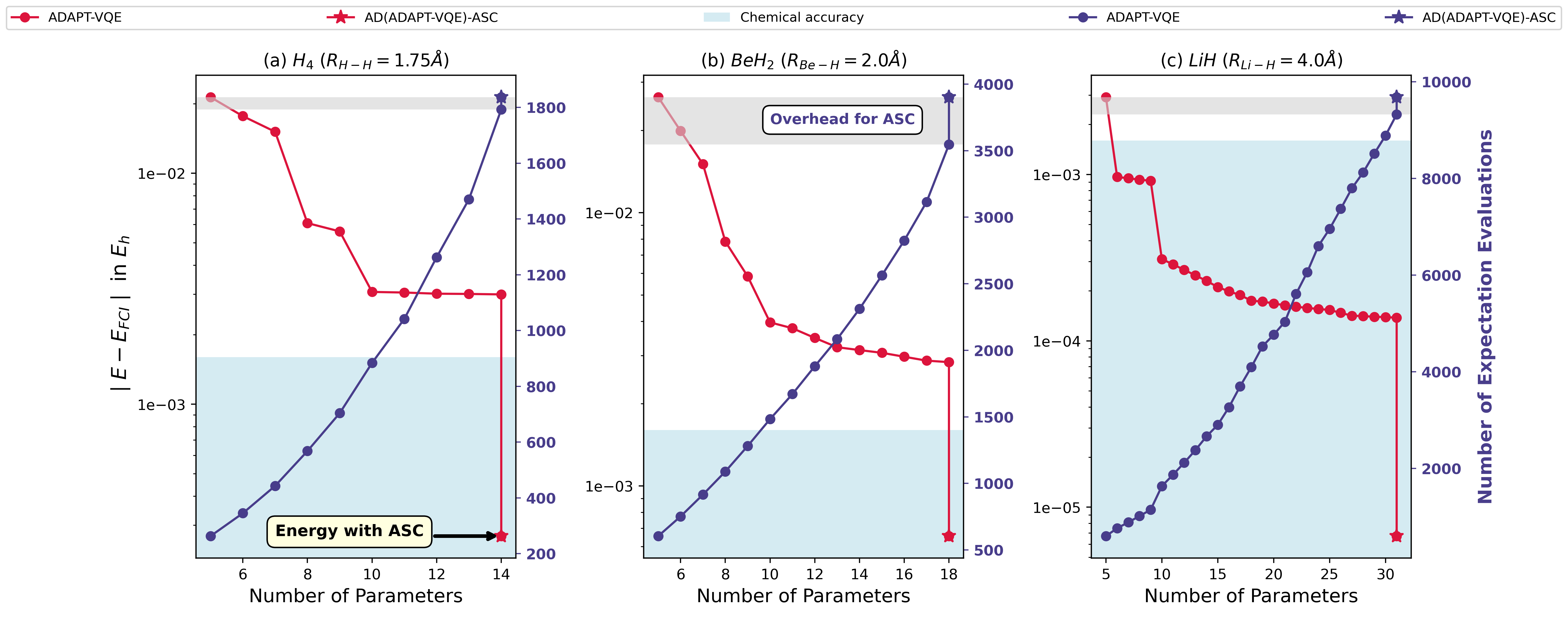
Figure 1: Energy optimization landscape for AD(ADAPT-VQE)-ASC with recycled initialization: The x-axis shows the number of parameters in the ansatz and the left y-axis corresponds to the logarithm of the difference in energy with FCI (the global minimum) for stretched geometries of (a) $H_{4}$ linear chain ($R_{H-H}=1.75\text{\AA }$), (b) $BeH_{2}$ ($R_{Be-H}=2.0\text{\AA }$) and (c) $LiH$ ($R_{Li-H}=4.0\text{\AA }$). The right y-axis shows the number of expectation evaluations that includes both gradient calculations for operator selection and function evaluations for optimization. The initial energy trajectory is for conventional ADAPT-VQE. Once the convergence criteria is met with the threshold $\epsilon=10^{-3}$, ADAPT-VQE exits the selection and optimization cycle and one-step ASC is performed at the last step. It shows the signature plummeting effect of ASC where energy reaches a more optimal minima for all the cases shown here. The corresponding measurement overhead for ASC is also shown in the grey shaded area along the right y-axis. The chemical accuracy is taken to be $1.6mE_{h}$ energy difference from FCI.

V Results and Discussion

In this section we will numerically demonstrate the superior performance and generailty of the theoretical framework developed so far in electronic structure problems. We will consider two methods: (1) ADAPT-VQE and (2) screened MP2-VQE to select the principal parameter space as discussed in section III. Our aim is to numerically study how effectively ASC can mitigate the effects of local minimas and provide more accurate results without utilising any significantly additional quantum or classical overhead. The results are obtained by in-house codes using python libraries and Qiskit[52]. The electronic integrals are imported from PySCF[53]. In case of ADAPT-VQE, we did not use the default Qiskit implementation of the same and the threshold ($\epsilon$) used here is not necessarily the same as that of the original paper[11]. The operator selection is done manually using the calculation of commutators along with the threshold criterion as described in Eq. (21) and (22). The subsequent VQE optimization is done using VQE function from Qiskit Nature with maximum iteration (maxiter) set to be 10,000. We have used L-BFGS-B and COBYLA optimizers for noiseless and noisy studies respectively. For all the calculations STO-6G basis set is used. Jordan-Wigner transformation is applied for the fermionic-to-qubit mapping. For all the simulations, the principal unitary was constructed from an operator pool consisting of singles and doubles (SD) excitations only. The auxiliary space contains the entire set of singles, doubles, triples and quadruples (SDTQ) operators. No symmetry considerations were used to reduce the qubit requirements.

The numerical discussion section is divided into three major sections. In Section V.1 we consider ADAPT-VQE as a tool for the principal subspace selection under noiseless scenarios. Section V.2 contains results with the screened MP2-VQE which is structurally more robust under hardware noise than measurement-based ansatz construction protocols. With screened MP2-VQE we discuss the effect of ASC under noisy circumstances as well. Finally in section VI we introduce a generator-informed initialization strategy for ADAPT-VQE that can lead to faster convergence.

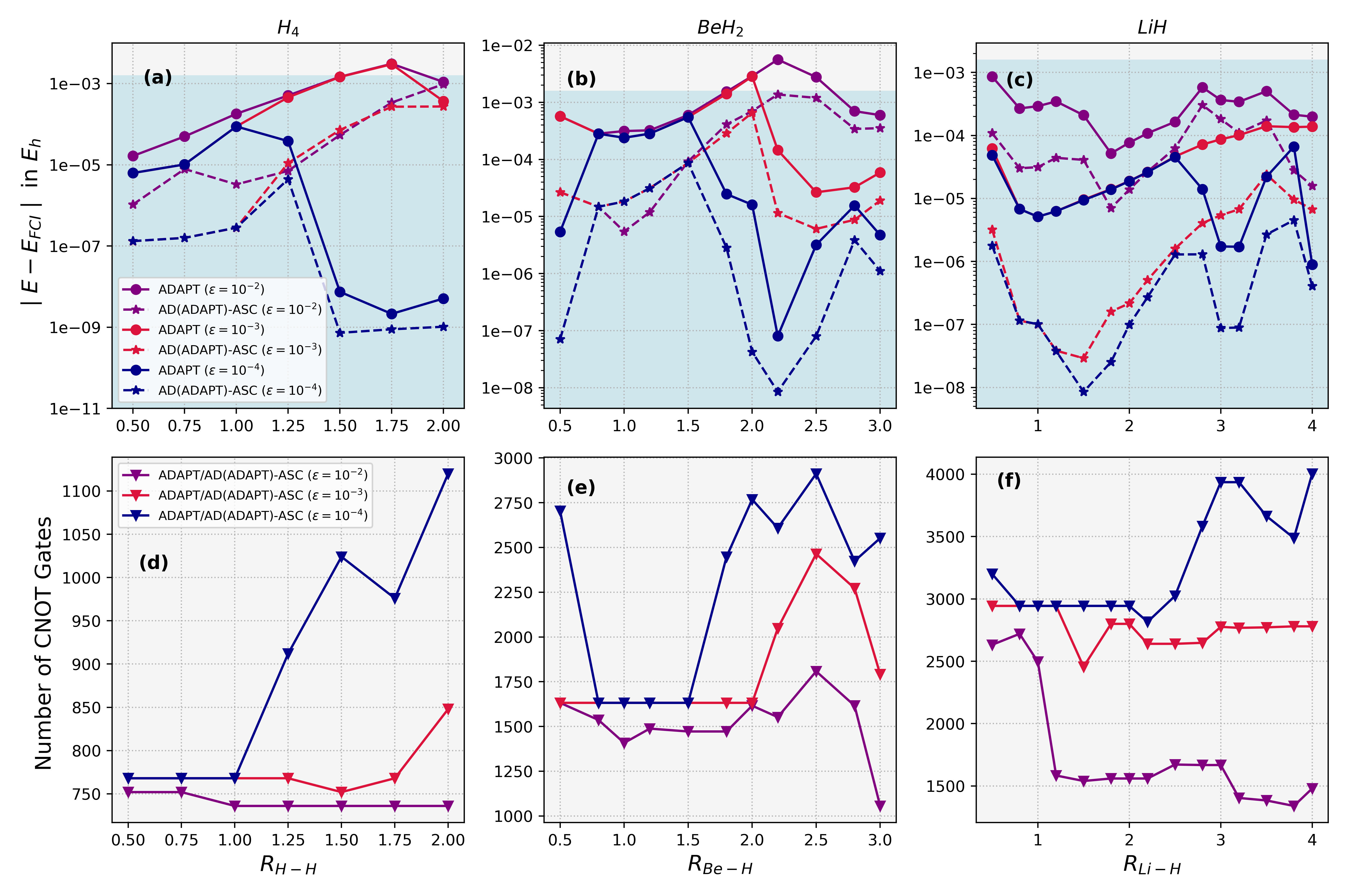
Figure 2: Comparison between ADAPT-VQE and AD(ADAPT-VQE)-ASC for different molecular geometries: The three columns are for linear $H_{4}$ chain, $BeH_{2}$ and $LiH$ molecule. Here y axes in all the subplots correspond to internuclear distances. The y-axes in (a), (b), (c) show the energy difference from FCI and (d), (e), (f) correspond to the associated number of CNOT gates. The solid and dotted lines correspond to ADAPT-VQE and AD(ADAPT-VQE)-ASC respectively with a specific threshold $\epsilon$. Note that AD(ADAPT-VQE)-ASC does not require additional CNOT gates in the circuit, so number of gates for it remains the same with ADAPT-VQE.

V.1 Principal Unitary Selection by X = ADAPT-VQE

In this section we use ADAPT-VQE as a tool to select the principal unitary which caters to an iterative construction of the ansatz to select important operators as discussed in details in section III.1. First we study some specific molecular configurations to demonstrate how ASC can partially mitigate the issue of local traps. Then we move over to the comparison between ADAPT-VQE and AD(ADAPT-VQE)-ASC for the entire potential energy profile of these systems.

V.1.1 Local Traps in Energy Optimization Landscape and ASC induced Plummeting Effect

Fig. 1 illustrates some typical energy optimization landscapes of AD(ADAPT-VQE)-ASC method for some molecular systems at their fixed internuclear geometries. Here the plot contains twin y-axis where the left y-axis represents the logarithm of energy difference of the methods under consideration in $E_{h}$ with respect to the global minimum obtained via full configuration interaction (FCI) calculation. Along the horizontal axis, the incremental number of parameters in the circuit is plotted. The right y-axes correspond to the number of expectation evaluations which includes both the number of gradient evaluations for operator selection and cost-function evaluations for the VQE optimizations. The threshold for the selection of the primary subspace via ADAPT-VQE was set to be $\epsilon=10^{-3}$ and each micro-iteration is initialized with recycled parameters.

Panel (a) of Figure 1 depicts the optimization landscape shown for linearly stretched $H_{4}$ chain ($R_{H-H}=1.75$Å) which reveals that ADAPT-VQE ($\epsilon=10^{-3}$) energy profile stagnates at a local minimum. This is evident as the energy trajectory shows no visible improvement over the last four operator selection cycles although they have non-vanishing gradient. However, once the convergence condition over the energy gradient (Eq. (22)) is met, the ASC is activated, significantly reducing the energy error from $3\times 10^{-3}E_{h}$ for ADAPT-VQE to $2\times 10^{-4}E_{h}$ which is well within the chemical accuracy. This corresponds to an accuracy improvement of more than an order of magnitude relative to the FCI energy. For $BeH_{2}$ (with $R_{Be-H}=2$Å) (Fig. 1(b)), ADAPT-VQE shows similar behavior while ASC still provides much better accuracy ($\sim 6\times 10^{-4}E_{h}$) compared to ADAPT-VQE ($\sim 3\times 10^{-3}E_{h}$). Similar trend is observed for $LiH$ ($R_{Li-H}=4$Å) where a local minima is still quite conspicuous toward the end of the ADAPT-VQE iterations. As analyzed previously, such improvements due to ASC requires no additional circuit resources such as CNOT gates or extra qubits, and only requires an insignificant number of additional gradient-like measurements (over the conventional choice of the method X where X=ADAPT-VQE in this section). Quantitatively, the number of extra gradient-like commutator expectation values is bounded by $\leq 2N_{A}$ as discussed in section IV. The grey shaded region along right y-axes in Fig. 1 shows the number of extra expectation values to be calculated which is proportional to the measurement overhead required for performing ASC. Evidently, this overhead (grey shaded region) is insignificant relative to total number of expectation evaluations. Interestingly, for a particular molecule in a given basis set, this overhead is invariant with respect to different geometries or different ADAPT-VQE threshold.

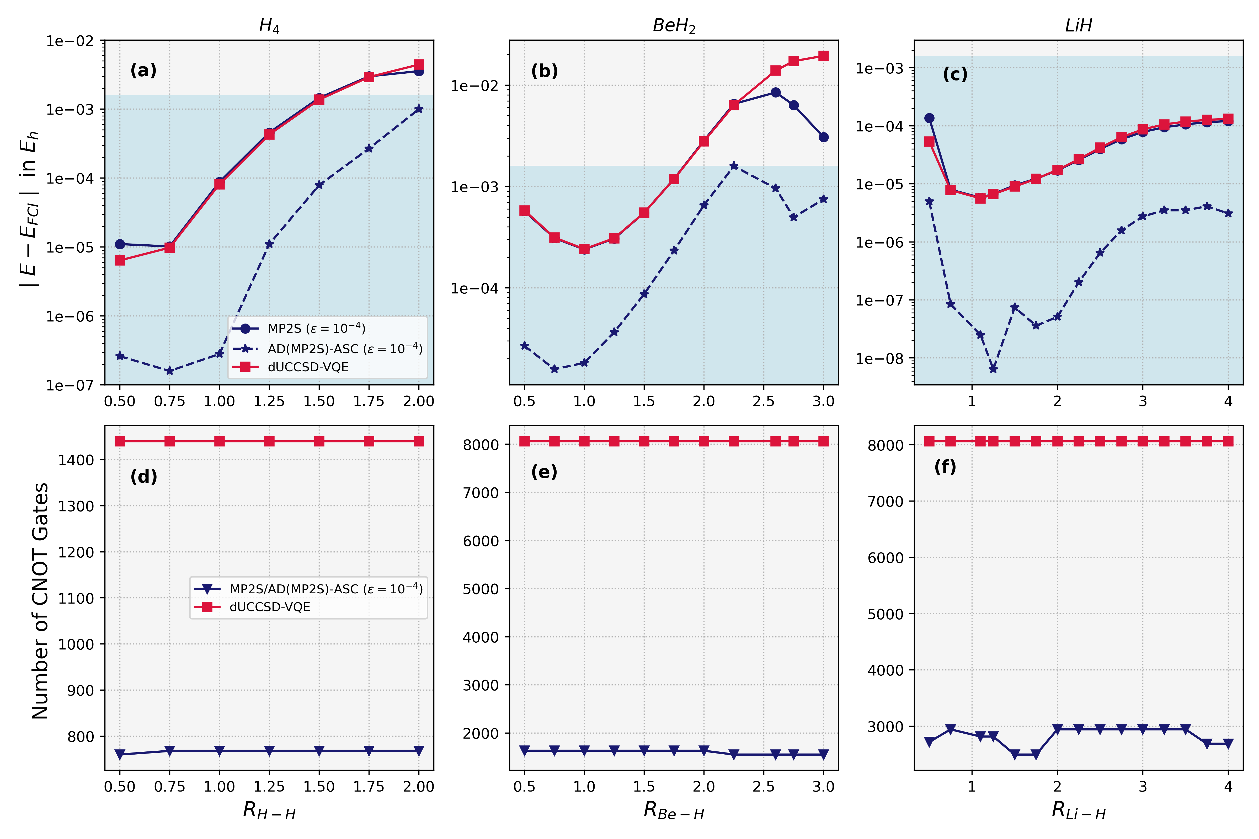
Figure 3: Comparison between MP2S-VQE and AD(MP2S-VQE)-ASC for different molecular geometries: The axes information are same as Fig. 2 with MP2S-VQE performed with only one threshold $\bar{\epsilon}=10^{-4}$. The dUCCSD energy and CNOT count values are also shown here for comparison. Note that the CNOT count for AD(MP2S-VQE)-ASC is same as MP2S-VQE.

In this context, it is worth noting that ADAPT-VQE can partially alleviate the challenge of local minima by progressively adding operators, enabling it to “burrow” into the parameter landscape [12]. However, this effect is most pronounced for very small values of $\epsilon$ with relatively more number of parameters, which typically leads to deeper circuits and excessively high measurement overhead. Our approach additionally achieves a one-step “plummeting effect”, reaching a significantly better optimal minimum even at higher $\epsilon$ values, all while maintaining the same number of parameters and circuit depth as that of ADAPT-VQE. Thus a combination of ADAPT-VQE (at a higher $\epsilon$ value) with ASC leads to extremely accurate energy estimation at much lower quantum resource requirements even with a set of recycled parameters, which can be significantly improved upon further with a generator-informed initialization (vide infra).

V.1.2 Accuracy Over the Potential Energy Surface: ADAPT-VQE vs AD(ADAPT-VQE)-ASC

In Fig. 2 we have studied the potential energy surfaces (PES) for all the molecules under consideration to assess the comparative behavior of ADAPT-VQE and AD(ADAPT-VQE)-ASC for different electronic complexities. Here we have considered ADAPT-VQE to select the principal subset with three different thresholds $\epsilon=10^{-2},10^{-3}$ and $10^{-4}$. In Fig. 2 ((a), (b), (c)) the logarithm of energy difference with respect to FCI (in $E_{h}$) is plotted in the y-axis while the x-axis represents different molecular bond distances in Å. Fig. 2 ((d), (e), (f)) represent the CNOT count for all different molecular geometries as a measure of quantum resource utilization. The solid lines and dashed lines represent ADAPT-VQE and AD(ADAPT-VQE)-ASC with purple, red and blue indicating $\epsilon$ values $10^{-2}$, $10^{-3}$ and $10^{-4}$ respectively. In Fig. 2 (a) for linear $H_{4}$ it is observed that AD(ADAPT-VQE)-ASC outperforms ADAPT-VQE in both weak and strong electronic correlation regime while providing one to two orders-of-magnitude better energy accuracy. The effect of ASC is so prominent that for near equilibrium geometries of linear $H_{4}$ chain (from $R_{H-H}=0.5$ to $R_{H-H}=1.25$Å), our method with $\epsilon=10^{-2}$ consistently provides visibly better accuracy than even ADAPT-VQE with $\epsilon=10^{-4}$. Similar trend is observed for symmetric bond stretching of $BeH_{2}$ as well where AD(ADAPT-VQE)-ASC always remains within the chemical accuracy window even if ADAPT-VQE struggles to achieve the same with $\epsilon=10^{-2}$ and $10^{-3}$ at around $R_{Be-H}=2.0\AA$. For $LiH$, AD(ADAPT-VQE)-ASC with $\epsilon=10^{-3}$ shows drastically more accurate results than ADAPT-VQE with $\epsilon=10^{-4}$ for both near equilibrium and stretched geometries (till $R_{Li-H}=2.8$Å). At $R_{Li-H}=3.8$Å, AD(ADAPT-VQE)-ASC with $\epsilon=10^{-2}$ provides $40\mu E_{h}$ better energy accuracy (dotted purple line) with respect to ADAPT-VQE with $\epsilon=10^{-4}$ (solid blue line) resulting in 61% reduction in CNOT gates. As theoretically argued and depicted in Fig. 2 (d), (e), (f), ADAPT-VQE and AD(ADAPT-VQE)-ASC both require same number of CNOT gates.

V.2 Principal Unitary Selection by X = Screened MP2-VQE (MP2S-VQE)

In this case we select the principal subspace via MP2 values and spin symmetry as discussed in section III.2. Here the potential energy surface is studied with noiseless simulations followed by noisy simulations to demonstrate the signature plummeting effect even under cases with realistic depolarising noise channels.

V.2.1 Potential Energy Surface Study

In Fig. 3 we have shown the case with X= screened MP2-VQE (MP2S-VQE). Here the principal subspace is formed by MP2 screened doubles with a threshold $\bar{\epsilon}=10^{-4}$ along with single excitations allowed by orbital-symmetry as discussed in section III.2. Results for disentangled UCC with singles and doubles (dUCCSD-VQE) are also shown for comparison with the default operator ordering as implemented in Qiskit. Since MP2S-VQE consists of dominant operators from SD pool, the results are identical with dUCCSD in most of the cases. However, for $BeH_{2}$ (plot (b) in Fig. 3) one can see in the stretched geometries (strong correlation region), MP2S-VQE and dUCCSD-VQE deviates slightly. This is most likely due to different operator ordering, dUCCSD-VQE gets stuck in a higher-energy local minima compared to MP2S-VQE. For all molecular cases studied here AD(MP2S-VQE)-ASC provides chemically accurate results even in the strong correlation regions where MP2S-VQE and dUCCSD-VQE suffer in terms of accuracy. For example, in the strongly correlated region for $BeH_{2}$ with $R_{Be-H}=2.75\text{\AA }$, MP2S-VQE and dUCCSD-VQE energy errors from FCI are $0.0064E_{h}$ and $0.017E_{h}$ respectively whereas, due to ASC this difference reduces to $0.0005E_{h}$. Similar trend is observed for linear $H_{4}$ and $LiH$ throughout the potential energy surface. In this case the parallelity of the errors over the PES for MP2S-VQE and AD(MP2S-VQE)-ASC is capable of providing consistent energy shift across PES.

To summarize, the numerical studies in this section suggests that AD(X)-ASC provides one to two orders of magnitude better accuracy than its conventional counterparts (i.e. method X) at a particular threshold even in the regions of molecular strong correlations where method X suffers to account for chemically accurate energies. This enhanced accuracy is obtained at a nominal overhead with $2N_{A}$ number of extra commutator measurements at worst and no additional circuit resources are required. Since the numerical simulations are noiseless in this section, in the next section we will discuss how quantum hardware noise affects such calculations.

V.2.2 Plummeting Effect under Noisy Simulations

For implementations in noisy hardware, as measurement based operator selection is unreliable due to the error-prone expectation value measurements, we opt for the MP2 based operator selection as discussed in section III.2. In Fig. 4 we have shown both noisy and noiseless simulations with MP2 based operator selection. The noisy simulations are done using only depolarising noise channels in Qiskit with two qubit gate error 0.01 and one qubit gate error 0.001 for linear $H_{4}$ chain with $H-H$ bond distance $1.5$Å. We have used CNOT-efficient circuits[21, 22] for this study to reduce number of CNOT gates. In addition to this, we have used Zero Noise Extrapolation[54] (ZNE) error mitigation technique. The value of the threshold ($\overline{\epsilon}$) regarding MP2 based selection is taken to be 0.05 (grey curve) and 0.1 (green curve) which selects 8 and 6 parameters respectively out of the 26 SD operators in the pool. Since in noisy simulations there is no notion of convergence, we terminated the simulations with 100 iterations for both noiseless and noisy studies to treat all the cases on an equal footing. The noisy plots are obtained by averaging over 100 independent runs and the corresponding standard deviations are shown with the shaded regions. Even for the noisy simulations, the signature dip in average energy as well as in the corresponding standard deviation due to ASC is discernible. It is important to note that the average energy for $\overline{\epsilon}=0.1$ is better than $\overline{\epsilon}=0.05$ under noise, which is counterintuitive as the former case has fewer parameters in the ansatz and hence ideally should be less accurate (as can be seen from the noiseless simulations in Fig. 4). This shows that the higher number of CNOT present in the circuit corresponding to $\overline{\epsilon}=0.05$ drives it away from the optimal solution due to the more disruptive signature of noise than the ansatz with $\overline{\epsilon}=0.1$. In such a case, it is still evident from Fig. 4 that the average energy (along with the standard deviation) with ASC for $\overline{\epsilon}=0.05$ is of the same order of the energy for $\overline{\epsilon}=0.1$ which shows the pronounced impact of ASC even under noisy scenarios.

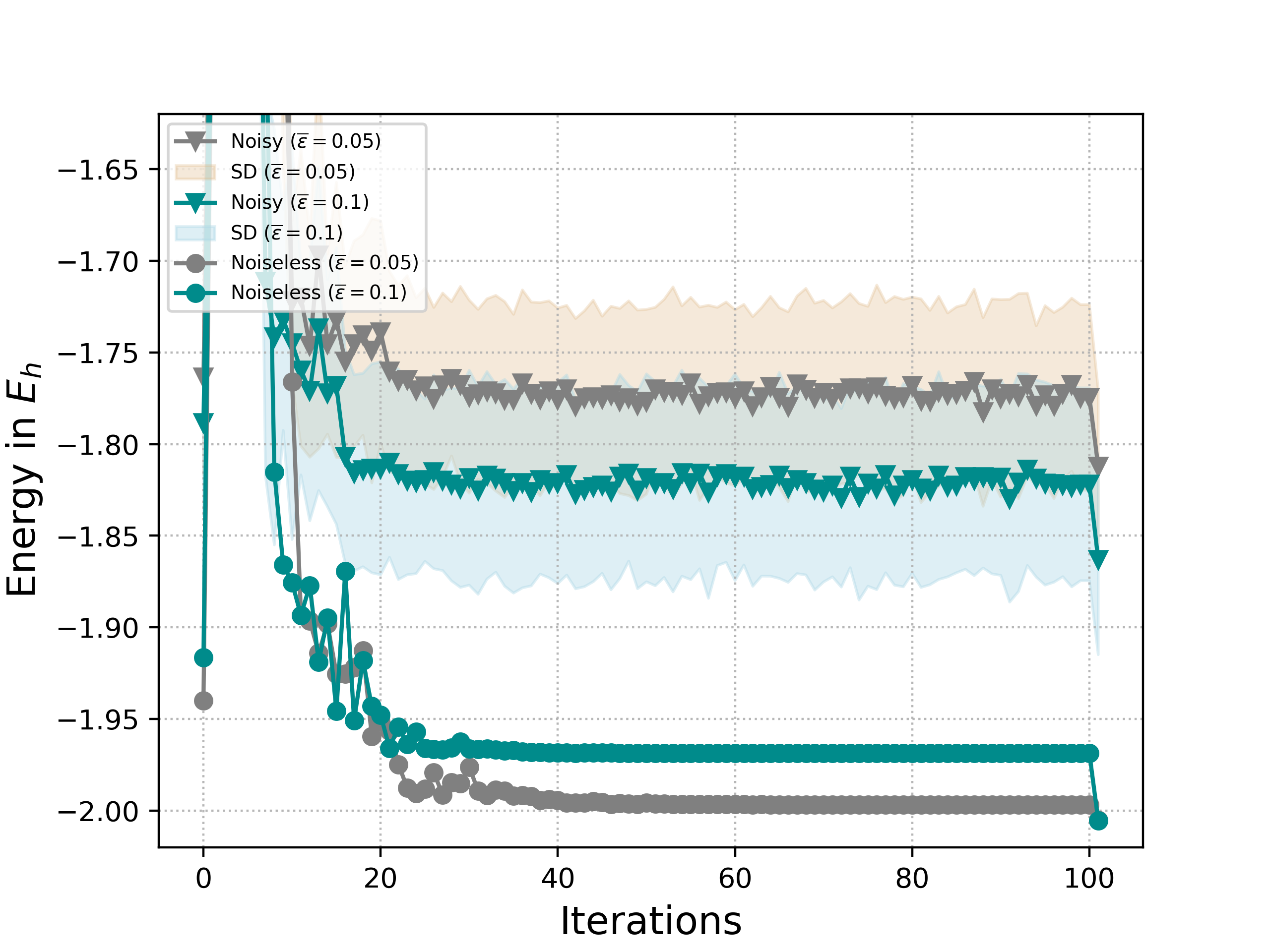
Figure 4: Noisy simulation: Simulation with depolarising noise channel for $H_{4}$ at $1.5\text{\AA }$ with principal space selection done by MP2 screening at different thresholds $\bar{\epsilon}$. Energy in $E_{h}$ is plotted in y-axis and x-axis corresponds to number of iterations. The corresponding noiseless simulations are also shown for better comprehension of the disruptive effects of noise.

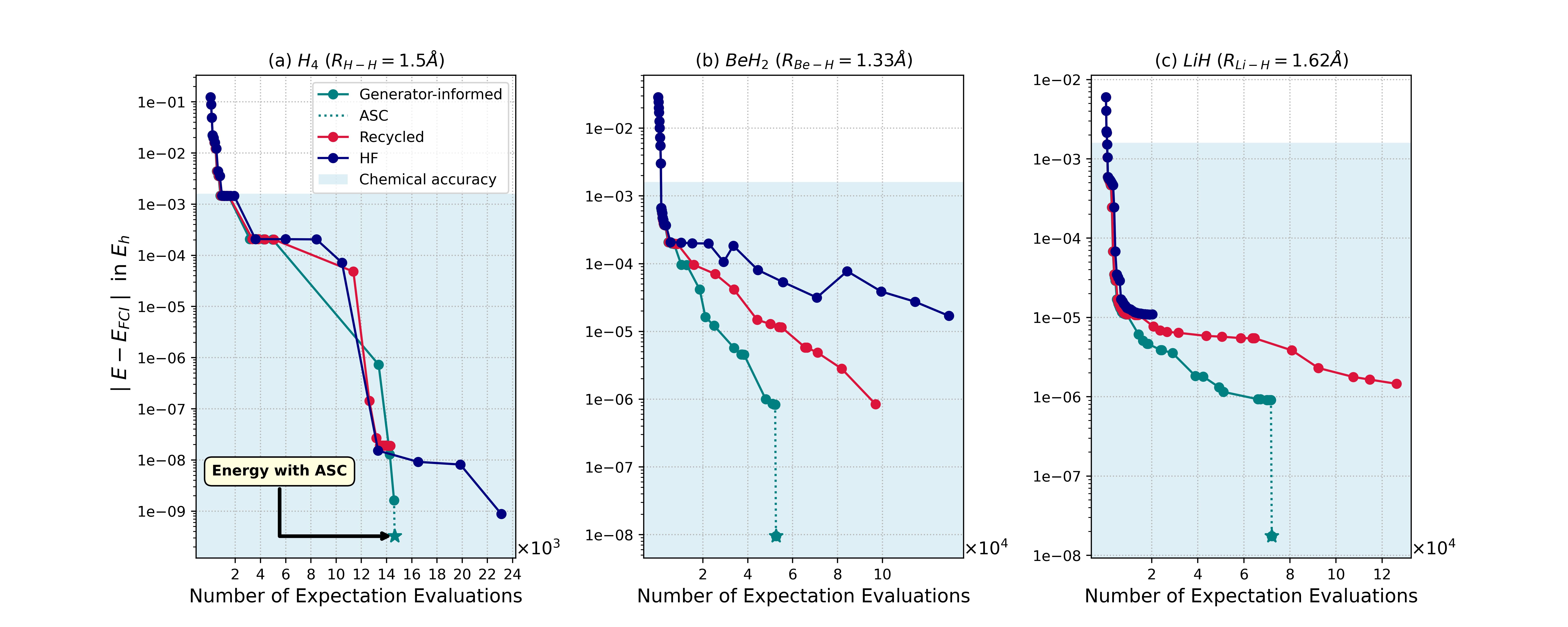
Figure 5: Comparison between generator-informed, recycled and HF initialization for ADAPT-VQE: Energy error (in logarithm scale) for ADAPT-VQE ($\epsilon=10^{-5}$) with respect to FCI is plotted as a function of the number of cost-function evaluations for three different molecules. The numerical studies suggest generator-informed initialization converges much faster compared to HF or recycled initializations. For both $BeH_{2}$ and $LiH$, the generator-informed initialization shows almost 50% reduction in number of function evaluations compared to recycled initialization. The ASC (dotted part of the green curve) leads to better minima with almost no additional quantum resources.

VI Generator-Informed Initialization Strategy for Improved ADAPT-VQE Optimization

Effective parameter initialization is one of the most crucial aspects for the trainability of PQCs and convergence of VQE calculations[55, 6, 2]. In cases where VQE cost-function landscapes flatten exponentially fast with the system size, initializing the optimization with random values of the parameters often get stuck in local traps or barren plateaus (BP)[4, 2]. Gradient descent-like algorithms can converge to any local minimum, mostly governed by the initialization[31, 56]. In general, if the initial guess of the parameters lies within the same local trap as that of the global minimum, then the classical optimizers seamlessly find the minimum. However, if this is not the case, then BPs obstruct the optimizer to escape the narrow gorge and it results in a sub-optimal solution[57]. Some recent studies show that parameter trainability can be enhanced via certain initialization techniques[34]. Thus, clever initialization strategies are one of the most promising ways to avoid BPs or local minimas since it jump start the training in a region of large gradients[6].

For molecular VQEs with UCC-like ansatze, the usual practice is to start with the physically motivated Hartree-Fock (HF) initializations where all the parameters start from zero (which corresponds to the HF solution) and the optimizations reach a nearly optimal minima in most cases. Grimsley et al. have recently suggested a “recycled” parameter initialization[12] strategy in ADAPT-VQE protocol where each VQE optimization starts with all the optimized values of the parameters in previous step along with the parameter corresponding to the new selected operator starting from zero (discussed in Section III.1). Such a recycled initialization was shown to perform better than HF initialization in some molecular-VQE applications.

Here we propose a new initialization strategy that stems from the notion of adiabatic decoupling. For a particular iteration, ADAPT-VQE selects the parameter with the largest gradient. Following the principles of adiabatic decoupling and mapping functional (Eq. (17)), at the $k$-th iteration, the newly added parameter can be approximated as a function of the previously optimized $(k-1)$ parameters. This yields an initial guess of the $k$-th parameter given by:

$$\theta_{P_{k}}^{init}\leftarrow-\frac{\bra{\Phi_{P}^{k-1}}[\hat{B},\hat{\mathcal{G}}_{P_{k}}]\ket{\Phi_{P}^{k-1}}}{\bra{\Phi_{P}^{k-1}}\Big{[}[\hat{B},\hat{\mathcal{G}}_{P_{k}}],\hat{\mathcal{G}}_{P_{k}}\Big{]}\ket{\Phi_{P}^{k-1}}}$$ (29)

where, $\ket{\Phi_{P}^{k-1}}$ is the ansatz formed at the end of the $(k-1)$-th macro-iteration step

$$\ket{\Phi_{P}^{k-1}}=\hat{U}_{P_{1}}^{\dagger}(\theta_{P_{1}}^{opt})..\hat{U}_{P_{k-1}}^{\dagger}(\theta_{P_{k-1}}^{opt})\ket{\Phi_{0}}.$$ (30)

with $[\theta_{P_{1}}^{opt},...\theta_{P_{k-1}}^{opt}]$ being the set of optimized parameters from $(k-1)$-th iteration. One may notice that Eq. (29) is structurally same as the principal-to-auxiliary mapping function (Eq. (17)). This implies that at the $k^{th}$ iteration, all the operators chosen till $(k-1)^{th}$ step is considered to span the principal parameter space and the $k^{th}$ operator chosen at the $k^{th}$ step is conceived as an auxiliary parameter which is subsequently added to the ansatz and it is initialized via Eq. (29) for further optimization. As the parameter initialization is driven by the corresponding generators, it will be referred to as “generator-informed” initialization. In the case of ADAPT-VQE with the new generator-informed initialization strategy, we warm-start each micro-iteration with the entire parameter set by the ($k-1$) optimized parameters from the previous step of the iteration along with the $k$-th parameter obtained via Eq. (29).

Though in this paper we discuss such generator-informed initialization strategy in the context of ADAPT-VQE only, the structure of Eq. (29) suggest that it is problem-independent and thus we hope it can be applicable to other optimization problems as well. We will explore more about such initialization strategies in forthcoming publications.

Emergence of Lower Energy Landscape Burrowing with Generator Informed Initialization

In Fig. 5 we have shown the energy convergence for ADAPT-VQE with $\epsilon=10^{-5}$ as a function of the number of expectation evaluations with three different initialization techniques: (i) generator-informed (green curve), (ii) recycled (red curve) and (iii) HF initialization (blue curve) as discussed in section VI. The numerical studies for (a) $H_{4}$ ($R_{H-H}=1.5$Å), (b) $LiH$ ($R_{Li-H}=1.33$Å) and (c) $BeH_{2}$ ($R_{Be-H}=1.62$Å) show that during the initial ADAPT-VQE macro-iteration cycles, all three types of parameter initialization techniques converge nearly to the same minima. However, the advantage of generator-informed initialization is more discernible as the number of parameters in the circuit increases since this amounts to a higher dimensional principal parameter subspace that are mapped to reconstruct auxiliary parameters. Consequently, one can see that for $BeH_{2}$, ADAPT-VQE with generator-informed initialization shows a 48% reduction in the overall number of expectation evaluations (which includes function evaluations and gradient calculations) to converge to similar energy minima compared to recycled initialization. Further, ASC provides almost two orders of magnitude more accurate energy minima (shown with an asterisk mark) at the cost of negligible amount of additional expectation calculations. For $H_{4}$, although the effect of generator-informed initialization is not markedly visible, the generator-informed initialization converges to slightly better minima. For $LiH$, generator-informed initialization reaches an energetically better minima with only half the amount of expectation evaluations required than other two initialization techniques.

In general, with generator-informed initialization for AD(ADAPT)-ASC, one obtains two-fold advantages: firstly, it is heuristically observed that the optimization trajectory finds a lower-energy “burrowing channel” that can potentially converge to lower energy minima compared to recycled or HF parameter initialization with significantly reduced quantum measurements. Secondly, the ASC leads to additional plummeting in the energy landscape without requiring any further quantum hardware resources, making the overall energy estimation extremely accurate.

VII Conclusion and Future Outlook

In this work, we introduce a formalism aimed at optimizing the trade-off between resource efficiency and accuracy in parameterized quantum circuits. Our approach conjectures the presence of a temporal hierarchy of the parameter optimization landscape which natuarally leads to the decoupling of the entire operator (parameter) space into a dominant principal and a recessive auxiliary subspace. Based upon this decoupling, the adiabatic approximation can be invoked by freezing the successive variation of the auxiliary parameters. Starting from the parameter-shift rule, adiabatic approximation leads to a principal-to-auxiliary mapping functional that enables the reconstruction of auxiliary parameters from optimized principal parameters only, leading to one-step auxiliary subspace corrections (ASC). This correction mechanism, implemented without introducing additional parameters into the PQC, ensures that circuit depth remains constrained to the principal subspace. Thus the correction terms factor in the approximate effects of the entire operator pool into the cost function towards a more optimal minima, without incurring any additional quantum resource overheads or classical optimization cycles which makes it an extremely resource efficient algorithm. Our AD(X)-ASC method, where “X” being the method to select and optimize the principal parameter subspace, is a general framework that can be applied to a wide class of optimization tasks.

In this paper, we have shown two different possible methods to choose “X”, namely ADAPT-VQE and MP2S-VQE to treat challenging electronic correlation effects for molecular cases like bond stretching in linear $H_{4}$ chain, $BeH_{2}$ and $LiH$. The numerical demonstrations show AD(ADAPT-VQE)-ASC and AD(MP2S-VQE)-ASC methods can provide upto two orders-of-magnitude better energy accuracy than both ADAPT-VQE and MP2S-VQE respectively, without any additional optimization or quantum circuit resources. The energy landscape study shows heuristic evidences that ASC exhibits a “plummeting” effect by which it can effectively alleviate local traps and reach a more optimal minima without requiring additional parameters in the PQC. The noisy simulations suggest that the signature plummeting effect in the energy landscape exists even under the disruptive behavior of noise which can be beneficial under the NISQ era of quantum computing. Additionally we have proposed a generator-informed initialization technique which is entirely guided by the generator of unitary rotations of the ansatz. Our numerical heuristics suggest this generator-informed initialization combined with ASC can lead to faster convergences by finding lower energy burrowing channels in the optimization landscape, followed by the characteristic ASC-aided plummeting for a more optimal energy minima estimation with less quantum measurement requirements compared to the conventional recycled or HF based parameter initialization techniques. From a general perspective, the structure of AD(X)-ASC shows promise that the optimization can be less affected by hardware noise as the optimization task is projected on to a lower dimensional manifold. Simultaneously, the problem of local traps, prevalent in shallow underparametrized circuits, is mitigated via generator-informed initialization along with ASC. However, this needs further investigation which will be the subject of our future publications.

VIII Acknowledgments

The authors acknowledge Ms. Dipanjali Halder for stimulating discussions. RM acknowledges the financial support from Industrial Research and Consultancy Centre (IRCC), IIT Bombay and Science and Engineering Research Board (SERB), Government of India (Grant Number: MTR/2023/001306). CP acknowledges University Grants Commission (UGC) for the fellowship.

AUTHOR DECLARATIONS

Conflict of Interest:

The authors have no conflict of interest to disclose.

Data Availability

The data is available upon reasonable request to the corresponding author.

Appendix A Second Order Approximation of the Cost Function

Starting from Eq. (13), we can explicitly apply BCH expansion for auxiliary part of the unitary

$$\begin{split}&f(\boldsymbol{\theta}\pm\frac{\pi}{2}\hat{e}_{A_{i}})=\bra{\Phi_{P}}\hat{B}\ket{\Phi_{P}}+(\theta_{A_{i}}\pm\frac{\pi}{2})\\ &\bra{\Phi_{P}}[\hat{B},\hat{\mathcal{G}}_{A_{i}}]\ket{\Phi_{P}}+\sum_{A_{j\neq i}}\theta_{A_{j}}\\ &\bra{\Phi_{P}}[\hat{B},\hat{\mathcal{G}}_{A_{j}}]\ket{\Phi_{P}}+\frac{1}{2}(\theta_{A_{i}}\pm\frac{\pi}{2})^{2}\\ &\bra{\Phi_{P}}\Big{[}[\hat{B},\hat{\mathcal{G}}_{A_{i}}],\hat{\mathcal{G}}_{A_{i}}\Big{]}\ket{\Phi_{P}}+\frac{1}{2}\sum_{A_{j}}\sum_{A_{k}\neq A_{i}}(\theta_{A_{j}}\pm\frac{\pi}{2}\delta_{A_{i}A_{j}})\theta_{A_{k}}\\ &\bra{\Phi_{P}}\Big{[}[\hat{B},\hat{\mathcal{G}}_{A_{j}}],\hat{\mathcal{G}}_{A_{k}}\Big{]}\ket{\Phi_{P}}+...\end{split}$$ (31)

which is a non-terminating series. Here the Kronecker-Delta function $\delta_{A_{i}A_{j}}$ ensures that the parameter-shift of $\frac{\pi}{2}$ only exists when $A_{j}$ is equal to $A_{i}$. Numerically the “non-diagonal” double commutators involving $\hat{\mathcal{G}}_{A_{j}}$ and $\hat{\mathcal{G}}_{A_{k}}$ along with the higher order terms in the series have negligible numerical contributions compared to the other leading order terms. Thus they can be ignored which leads to the approximated Eq. (14).

Appendix B Principal-to-Auxiliary Mapping from Parameter-Shift Rule

One can directly plug the full BCH expansion in Eq. (31) into the Parameter-shift rule for auxiliary gradient calculations (Eq. (12))

$$\begin{split}&\Delta\theta_{A_{i}}=\frac{1}{2}\Big{[}f(\boldsymbol{\theta}+\frac{\pi}{2}\hat{e}_{A_{i}})-f(\boldsymbol{\theta}-\frac{\pi}{2}\hat{e}_{A_{i}})\Big{]}\\ &=\frac{1}{2}\Big{[}\Big{(}\frac{\pi}{2}\bra{\Phi_{P}}[\hat{B},\hat{\mathcal{G}}_{A_{i}}]\ket{\Phi_{P}}+\theta_{A_{i}}.\frac{\pi}{2}\\ &\bra{\Phi_{P}}\Big{[}[\hat{B},\hat{\mathcal{G}}_{A_{i}}],\hat{\mathcal{G}}_{A_{i}}\Big{]}\ket{\Phi_{P}}+\frac{1}{2}\sum_{A_{k}\neq A_{i}}(\theta_{A_{i}}+\frac{\pi}{2})\theta_{A_{k}}\\ &\bra{\Phi_{P}}\Big{[}[\hat{B},\hat{\mathcal{G}}_{A_{i}}],\hat{\mathcal{G}}_{A_{k}}\Big{]}\ket{\Phi_{P}}+...\Big{)}-\Big{(}-\frac{\pi}{2}\bra{\Phi_{P}}[\hat{B},\hat{\mathcal{G}}_{A_{i}}]\ket{\Phi_{P}}\\ &-\theta_{A_{i}}.\frac{\pi}{2}\bra{\Phi_{P}}\Big{[}[\hat{B},\hat{\mathcal{G}}_{A_{i}}],\hat{\mathcal{G}}_{A_{i}}\Big{]}\ket{\Phi_{P}}\\ &+\frac{1}{2}\sum_{A_{k}\neq A_{i}}(\theta_{A_{i}}-\frac{\pi}{2})\theta_{A_{k}}\bra{\Phi_{P}}\Big{[}[\hat{B},\hat{\mathcal{G}}_{A_{i}}],\hat{\mathcal{G}}_{A_{k}}\Big{]}\ket{\Phi_{P}}+...\Big{)}\Big{]}\end{split}$$ (32)

where, all the other terms are identical in both $f(\boldsymbol{\theta}+\frac{\pi}{2}\hat{e}_{A_{i}})$ and $f(\boldsymbol{\theta}-\frac{\pi}{2}\hat{e}_{A_{i}})$ and thus all of them cancel out. One can simplify Eq. (LABEL:delta_theta_A_expanded_full) further into

$$\begin{split}&\Delta\theta_{A_{i}}=\frac{\pi}{2}\Big{[}\bra{\Phi_{P}}[\hat{B},\hat{\mathcal{G}}_{A_{i}}]\ket{\Phi_{P}}\\ &+\theta_{A_{i}}\bra{\Phi_{P}}\Big{[}[\hat{B},\hat{\mathcal{G}}_{A_{i}}],\hat{\mathcal{G}}_{A_{i}}\Big{]}\ket{\Phi_{P}}\\ &+\frac{1}{2}\sum_{A_{k}\neq A_{i}}\theta_{A_{k}}\bra{\Phi_{P}}\Big{[}[\hat{B},\hat{\mathcal{G}}_{A_{i}}],\hat{\mathcal{G}}_{A_{k}}\Big{]}\ket{\Phi_{P}}+...\Big{]}\end{split}$$ (33)

In Eq. (LABEL:Delta_theta_A_before_final_approx) the terms involving “non-diagonal” double commutators with $\hat{\mathcal{G}}_{A_{i}}$ and $\hat{\mathcal{G}}_{A_{k}}$ are ignored since in general such terms are extremely small with respect to other leading order terms. Moreover, retaining such terms would lead to additional measurement overhead. Combined with the adiabatic approximation, this provides us with

$$\begin{split}&\Delta\theta_{A_{i}}\approx\frac{\pi}{2}\Big{[}\bra{\Phi_{P}}[\hat{B},\hat{\mathcal{G}}_{A_{i}}]\ket{\Phi_{P}}\\ &+\theta_{A_{i}}\bra{\Phi_{P}}\Big{[}[\hat{B},\hat{\mathcal{G}}_{A_{i}}],\hat{\mathcal{G}}_{A_{i}}\Big{]}\ket{\Phi_{P}}\Big{]}=0\end{split}$$ (34)

which leads to the principal-to-auxiliary mapping functional (Eq. (17)). Similar approximation is used to obtain the expression for the approximate cost function with ASC (Eq. (19)).

References:

References

- Peruzzo et al. [2014] A. Peruzzo, J. McClean, P. Shadbolt, M.-H. Yung, X.-Q. Zhou, P. J. Love, A. Aspuru-Guzik, and J. L. O’brien, “A variational eigenvalue solver on a photonic quantum processor,” Nature communications 5, 4213 (2014).
- Cerezo et al. [2021a] M. Cerezo, A. Arrasmith, R. Babbush, S. C. Benjamin, S. Endo, K. Fujii, J. R. McClean, K. Mitarai, X. Yuan, L. Cincio, et al., “Variational quantum algorithms,” Nature Reviews Physics 3, 625–644 (2021a).
- Bharti et al. [2022] K. Bharti, A. Cervera-Lierta, T. H. Kyaw, T. Haug, S. Alperin-Lea, A. Anand, M. Degroote, H. Heimonen, J. S. Kottmann, T. Menke, et al., “Noisy intermediate-scale quantum algorithms,” Reviews of Modern Physics 94, 015004 (2022).
- McClean et al. [2018] J. R. McClean, S. Boixo, V. N. Smelyanskiy, R. Babbush, and H. Neven, “Barren plateaus in quantum neural network training landscapes,” Nature communications 9, 4812 (2018).
- Cerezo et al. [2021b] M. Cerezo, A. Sone, T. Volkoff, L. Cincio, and P. J. Coles, “Cost function dependent barren plateaus in shallow parametrized quantum circuits,” Nature communications 12, 1791 (2021b).
- Larocca et al. [2025] M. Larocca, S. Thanasilp, S. Wang, K. Sharma, J. Biamonte, P. J. Coles, L. Cincio, J. R. McClean, Z. Holmes, and M. Cerezo, “Barren plateaus in variational quantum computing,” Nature Reviews Physics , 1–16 (2025).
- Anschuetz and Kiani [2022] E. R. Anschuetz and B. T. Kiani, “Quantum variational algorithms are swamped with traps,” Nature Communications 13, 7760 (2022).
- Larocca et al. [2023] M. Larocca, N. Ju, D. García-Martín, P. J. Coles, and M. Cerezo, “Theory of overparametrization in quantum neural networks,” Nature Computational Science 3, 542–551 (2023).
- Kiani, Lloyd, and Maity [2020] B. T. Kiani, S. Lloyd, and R. Maity, “Learning unitaries by gradient descent,” arXiv preprint arXiv:2001.11897 (2020).
- Wiersema et al. [2020] R. Wiersema, C. Zhou, Y. de Sereville, J. F. Carrasquilla, Y. B. Kim, and H. Yuen, “Exploring entanglement and optimization within the hamiltonian variational ansatz,” PRX quantum 1, 020319 (2020).
- Grimsley et al. [2019] H. R. Grimsley, S. E. Economou, E. Barnes, and N. J. Mayhall, “An adaptive variational algorithm for exact molecular simulations on a quantum computer,” Nature communications 10, 3007 (2019).
- Grimsley et al. [2023] H. R. Grimsley, G. S. Barron, E. Barnes, S. E. Economou, and N. J. Mayhall, “Adaptive, problem-tailored variational quantum eigensolver mitigates rough parameter landscapes and barren plateaus,” npj Quantum Information 9 (2023).
- Tang et al. [2021] H. L. Tang, V. Shkolnikov, G. S. Barron, H. R. Grimsley, N. J. Mayhall, E. Barnes, and S. E. Economou, “qubit-adapt-vqe: An adaptive algorithm for constructing hardware-efficient ansätze on a quantum processor,” PRX Quantum 2, 020310 (2021).
- Yordanov et al. [2021] Y. S. Yordanov, V. Armaos, C. H. Barnes, and D. R. Arvidsson-Shukur, “Qubit-excitation-based adaptive variational quantum eigensolver,” Communications Physics 4, 228 (2021).
- Zhu et al. [2022] L. Zhu, H. L. Tang, G. S. Barron, F. Calderon-Vargas, N. J. Mayhall, E. Barnes, and S. E. Economou, “Adaptive quantum approximate optimization algorithm for solving combinatorial problems on a quantum computer,” Physical Review Research 4, 033029 (2022).
- Mondal et al. [2023] D. Mondal, D. Halder, S. Halder, and R. Maitra, “Development of a compact Ansatz via operator commutativity screening: Digital quantum simulation of molecular systems,” The Journal of Chemical Physics 159, 014105 (2023).
- Halder, Prasannaa, and Maitra [2022] D. Halder, V. S. Prasannaa, and R. Maitra, “Dual exponential coupled cluster theory: Unitary adaptation, implementation in the variational quantum eigensolver framework and pilot applications,” The Journal of Chemical Physics 157, 174117 (2022).
- Stair and Evangelista [2021] N. H. Stair and F. A. Evangelista, “Simulating many-body systems with a projective quantum eigensolver,” PRX Quantum 2, 030301 (2021).
- Ryabinkin et al. [2018] I. G. Ryabinkin, T.-C. Yen, S. N. Genin, and A. F. Izmaylov, “Qubit coupled cluster method: a systematic approach to quantum chemistry on a quantum computer,” Journal of chemical theory and computation 14, 6317–6326 (2018).
- Ryabinkin et al. [2020] I. G. Ryabinkin, R. A. Lang, S. N. Genin, and A. F. Izmaylov, “Iterative qubit coupled cluster approach with efficient screening of generators,” Journal of chemical theory and computation 16, 1055–1063 (2020).
- Yordanov, Arvidsson-Shukur, and Barnes [2020] Y. S. Yordanov, D. R. Arvidsson-Shukur, and C. H. Barnes, “Efficient quantum circuits for quantum computational chemistry,” Physical Review A 102, 062612 (2020).
- Magoulas and Evangelista [2023a] I. Magoulas and F. A. Evangelista, “Cnot-efficient circuits for arbitrary rank many-body fermionic and qubit excitations,” Journal of Chemical Theory and Computation 19, 822–836 (2023a).
- Mondal et al. [2024] D. Mondal, C. Patra, D. Halder, and R. Maitra, “Projective quantum eigensolver with generalized operators,” arXiv preprint arXiv:2410.16111 (2024).
- Patra et al. [2024] C. Patra, D. Mukherjee, S. Halder, D. Mondal, and R. Maitra, “Toward a resource-optimized dynamic quantum algorithm via non-iterative auxiliary subspace corrections,” The Journal of Chemical Physics 161 (2024).
- Halder et al. [2023a] D. Halder, S. Halder, D. Mondal, C. Patra, A. Chakraborty, and R. Maitra, “Corrections beyond coupled cluster singles and doubles through selected generalized rank-two operators: digital quantum simulation of strongly correlated systems,” Journal of Chemical Sciences 135, 41 (2023a).
- Halder, Mondal, and Maitra [2024] D. Halder, D. Mondal, and R. Maitra, “Noise-independent route toward the genesis of a compact ansatz for molecular energetics: A dynamic approach,” The Journal of Chemical Physics 160 (2024).
- Halder et al. [2024] S. Halder, A. Dey, C. Shrikhande, and R. Maitra, “Machine learning assisted construction of a shallow depth dynamic ansatz for noisy quantum hardware,” Chemical Science 15, 3279–3289 (2024).
- Kowalski [2021] K. Kowalski, “Dimensionality reduction of the many-body problem using coupled-cluster subsystem flow equations: Classical and quantum computing perspective,” Physical Review A 104, 032804 (2021).
- Kowalski and Bauman [2023] K. Kowalski and N. P. Bauman, “Quantum flow algorithms for simulating many-body systems on quantum computers,” Physical Review Letters 131, 200601 (2023).
- Robledo-Moreno et al. [2024] J. Robledo-Moreno, M. Motta, H. Haas, A. Javadi-Abhari, P. Jurcevic, W. Kirby, S. Martiel, K. Sharma, S. Sharma, T. Shirakawa, et al., “Chemistry beyond exact solutions on a quantum-centric supercomputer,” arXiv preprint arXiv:2405.05068 (2024).
- Bittel and Kliesch [2021] L. Bittel and M. Kliesch, “Training variational quantum algorithms is np-hard,” Physical review letters 127, 120502 (2021).
- Holmes et al. [2022] Z. Holmes, K. Sharma, M. Cerezo, and P. J. Coles, “Connecting ansatz expressibility to gradient magnitudes and barren plateaus,” PRX Quantum 3, 010313 (2022).
- Grant et al. [2019] E. Grant, L. Wossnig, M. Ostaszewski, and M. Benedetti, “An initialization strategy for addressing barren plateaus in parametrized quantum circuits,” Quantum 3, 214 (2019).
- Wang et al. [2024] Y. Wang, B. Qi, C. Ferrie, and D. Dong, “Trainability enhancement of parameterized quantum circuits via reduced-domain parameter initialization,” Physical Review Applied 22, 054005 (2024).
- Patra, Halder, and Maitra [2024] C. Patra, S. Halder, and R. Maitra, “Projective quantum eigensolver via adiabatically decoupled subsystem evolution: A resource efficient approach to molecular energetics in noisy quantum computers,” The Journal of Chemical Physics 160 (2024).
- Halder et al. [2023b] S. Halder, C. Patra, D. Mondal, and R. Maitra, “Machine learning aided dimensionality reduction toward a resource efficient projective quantum eigensolver: Formal development and pilot applications,” The Journal of Chemical Physics 158 (2023b).
- Agarawal, Chakraborty, and Maitra [2020] V. Agarawal, A. Chakraborty, and R. Maitra, “Stability analysis of a double similarity transformed coupled cluster theory,” The Journal of Chemical Physics 153, 084113 (2020).
- Agarawal et al. [2021] V. Agarawal, S. Roy, A. Chakraborty, and R. Maitra, “Accelerating coupled cluster calculations with nonlinear dynamics and supervised machine learning,” The Journal of Chemical Physics 154, 044110 (2021).
- Agarawal, Patra, and Maitra [2021] V. Agarawal, C. Patra, and R. Maitra, “An approximate coupled cluster theory via nonlinear dynamics and synergetics: The adiabatic decoupling conditions,” The Journal of Chemical Physics 155, 124115 (2021).
- Patra et al. [2023] C. Patra, V. Agarawal, D. Halder, A. Chakraborty, D. Mondal, S. Halder, and R. Maitra, “A synergistic approach towards optimization of coupled cluster amplitudes by exploiting dynamical hierarchy,” ChemPhysChem 24, e202200633 (2023).
- Mitarai et al. [2018] K. Mitarai, M. Negoro, M. Kitagawa, and K. Fujii, “Quantum circuit learning,” Physical Review A 98, 032309 (2018).
- Schuld et al. [2019] M. Schuld, V. Bergholm, C. Gogolin, J. Izaac, and N. Killoran, “Evaluating analytic gradients on quantum hardware,” Physical Review A 99, 032331 (2019).
- Wierichs et al. [2022] D. Wierichs, J. Izaac, C. Wang, and C. Y.-Y. Lin, “General parameter-shift rules for quantum gradients,” Quantum 6, 677 (2022).
- Van Kampen [1985] N. G. Van Kampen, “Elimination of fast variables,” Physics Reports 124, 69–160 (1985).
- Claudino et al. [2021] D. Claudino, B. Peng, N. P. Bauman, K. Kowalski, and T. S. Humble, “Improving the accuracy and efficiency of quantum connected moments expansions,” Quantum Science and Technology 6, 034012 (2021).
- Magoulas and Evangelista [2023b] I. Magoulas and F. A. Evangelista, “Unitary coupled cluster: Seizing the quantum moment,” The Journal of Physical Chemistry A 127, 6567–6576 (2023b).
- Windom, Claudino, and Bartlett [2024] Z. W. Windom, D. Claudino, and R. J. Bartlett, “A new "gold standard": Perturbative triples corrections in unitary coupled cluster theory and prospects for quantum computing,” The Journal of Chemical Physics 160 (2024).
- Haidar et al. [2024] M. Haidar, O. Adjoua, S. Badreddine, A. Peruzzo, and J.-P. Piquemal, “Non-iterative disentangled unitary coupled-cluster based on lie-algebraic structure,” Quantum Science and Technology (2024).
- Kowalski [2018] K. Kowalski, “Properties of coupled-cluster equations originating in excitation sub-algebras,” The Journal of Chemical Physics 148, 094104 (2018).
- Kowalski, Brabec, and Peng [2018] K. Kowalski, J. Brabec, and B. Peng, “Regularized and renormalized many-body techniques for describing correlated molecular systems: A Coupled-Cluster perspective,” Annual Reports in Computational Chemistry 14, 3–45 (2018).
- Evangelista, Chan, and Scuseria [2019] F. A. Evangelista, G. K.-L. Chan, and G. E. Scuseria, “Exact parameterization of fermionic wave functions via unitary coupled cluster theory,” The Journal of Chemical Physics 151, 244112 (2019), https://pubs.aip.org/aip/jcp/article-pdf/doi/10.1063/1.5133059/16659468/244112_1_online.pdf .
- Javadi-Abhari et al. [2024] A. Javadi-Abhari, M. Treinish, K. Krsulich, C. J. Wood, J. Lishman, J. Gacon, S. Martiel, P. D. Nation, L. S. Bishop, A. W. Cross, B. R. Johnson, and J. M. Gambetta, “Quantum computing with Qiskit,” (2024), arXiv:2405.08810 [quant-ph] .
- Sun et al. [2018] Q. Sun, T. C. Berkelbach, N. S. Blunt, G. H. Booth, S. Guo, Z. Li, J. Liu, J. D. McClain, E. R. Sayfutyarova, S. Sharma, et al., “Pyscf: the python-based simulations of chemistry framework,” Wiley Interdisciplinary Reviews: Computational Molecular Science 8, e1340 (2018).
- Giurgica-Tiron et al. [2020] T. Giurgica-Tiron, Y. Hindy, R. LaRose, A. Mari, and W. J. Zeng, “Digital zero noise extrapolation for quantum error mitigation,” in 2020 IEEE International Conference on Quantum Computing and Engineering (QCE) (IEEE, 2020) pp. 306–316.
- Zhou et al. [2020] L. Zhou, S.-T. Wang, S. Choi, H. Pichler, and M. D. Lukin, “Quantum approximate optimization algorithm: Performance, mechanism, and implementation on near-term devices,” Physical Review X 10, 021067 (2020).
- Wierichs, Gogolin, and Kastoryano [2020] D. Wierichs, C. Gogolin, and M. Kastoryano, “Avoiding local minima in variational quantum eigensolvers with the natural gradient optimizer,” Physical Review Research 2, 043246 (2020).
- Mao, Tian, and Sun [2024] R. Mao, G. Tian, and X. Sun, “Towards determining the presence of barren plateaus in some chemically inspired variational quantum algorithms,” Communications Physics 7, 342 (2024).