DESY-25-064

Perturbed symmetric-product orbifold: first-order mixing and puzzles for integrability

Matheus Fabri^1,2$\star$, Alessandro Sfondrini^1,2$\dagger$ and Torben Skrzypek^{1,3$\ddagger$}

Abstract

We study the marginal deformation of the symmetric-product orbifold theory Sym${}_{N}(T^{4})$ which corresponds to introducing a small amount of Ramond-Ramond flux into the dual $AdS_{3}\times S^{3}\times T^{4}$ background. Already at first order in perturbation theory, the dimension of certain single-cycle operators is corrected, indicating that wrapping corrections from integrability must come into play earlier than expected. We also discuss a flaw in the original derivation of the integrable structure of the perturbed orbifold. Together, these observations suggest that more needs to be done to correctly identify and exploit the integrable structure of the perturbed orbifold CFT.

 

Contents

1. 1 Introduction
2. 2 The (deformed) symmetric-product orbifold in a nutshell
   1. 2.1 Definition of the unperturbed orbifold
   2. 2.2 Correlation functions, covering maps, and lifting
   3. 2.3 Spectrum before the perturbation
   4. 2.4 Marginal deformation
3. 3 First-order perturbation theory and mixing matrices
   1. 3.1 Conformal perturbation theory and Sym${}_{N}(T^{4})$
   2. 3.2 Constructing the mixing matrix elements
      1. 3.2.1 Twist field contribution
      2. 3.2.2 Boson contribution
      3. 3.2.3 Fermion contribution and bosonisation
   3. 3.3 Anomalous dimensions for light states
4. 4 Relation to integrability
   1. 4.1 Order-$\lambda$ mixing matrix in the $w\to\infty$ limit
   2. 4.2 Comments on the large-$w$ analysis of [18]
   3. 4.3 Order-$\lambda$ anomalous dimensions at finite $w$ from integrability
5. 5 Conclusions and outlook
6. A Conventions for the seed theory
7. B Currents and charges of the symmetric-product orbifold
8. C Details on the chiral ring
9. D Integrated Wick contractions
10. E Bosonisation in covering space

 

1 Introduction

The symmetric-product orbifold CFT of $T^{4}$ plays an important role in the AdS3/CFT2 correspondence [1]. It is dual to type IIB string theory on $AdS_{3}\times S^{3}\times T^{4}$ background supported by precisely $k=1$ units of Neveu-Schwarz-Neveu-Schwarz (NSNS) flux [2, 3, 4]. Because this is a free model, it is possible to compute in detail many of the observables of the theory. However, such computations become substantially more complicated when adding Ramond-Ramond (RR) background flux to the setup. This continuous change of the string background (which can be achieved by turning on an axion, see e.g. [5]) corresponds to a specific marginal deformation in the symmetric-product orbifold CFT, see e.g. [6, 7].

On the string side, it is notoriously difficult to quantise the worldsheet theory in the presence of RR fluxes. If the Green-Schwarz (GS) action for a given background is classically integrable, one can try to quantise it in lightcone gauge and solve the theory in terms of a factorised S matrix on the worldsheet, following [8] — an approach which has proven remarkably powerful for the study of $AdS_{5}\times S^{5}$ superstrings, see [9, 10]. Remarkably, the GS action for strings on $AdS_{3}\times S^{3}\times T^{4}$ with mixed NSNS/RR flux is classically integrable [11]. This spurred an active interest in constructing the quantum S matrix on the string worldsheet by integrable bootstrap approaches, and using it to compute the spectrum of the model (see [12, 13, 14] for reviews of various aspects of this construction).

At the same time, it was long conjectured that an integrable structure (perhaps similar to that of the $\mathcal{N}=4$ supersymmetric Yang-Mills theory [15]) should appear in the marginally-deformed symmetric-orbifold CFT [16, 17]. A recent development was the purported identification of the symmetry algebra expected from worldsheet integrability in the symmetric-product orbifold theory [18]. After correcting the identification of representations, which was done in [19], such an algebra reproduces the S matrix known from the worldsheet-integrability construction [20].

The purpose of this paper is to explore marginally-deformed symmetric-orbifold CFT and in particular its spectrum. More specifically, we will be interested in the anomalous dimensions of single-cycle operators (which can be thought of as the analogues of single-trace operators in $\mathcal{N}=4$ SYM) in the planar limit. Calling $\lambda$ the marginal coupling, the anomalous dimension of most operators will be of order $O(\lambda^{2})$, as it has been found by conformal perturbation theory in a number of cases, see e.g. [21, 22, 23, 24, 25, 26, 27, 28]. However, a relatively small subset of states will receive corrections of order $O(\lambda)$, as we shall see. These pose a challenge for the integrability approach, where (as least naïvely) one would also expect states to be corrected at $O(\lambda^{2})$. Below we will work out these corrections in detail and point out their relevance to the integrability construction, and in particular to finite-volume (“wrapping”) corrections, which are their most likely explanation.

In the course of this computation we will also revisit the construction of [18] which identified the integrability structure in the deformed symmetric-orbifold CFT. Surprisingly, we find an apparent flaw in that derivation which calls into question its conclusions. This issue is different from the mismatch in the identification of the representations already pointed out in [19].

This paper is structured as follows: we start by reviewing the symmetric-product orbifold theory Sym${}_{N}(T^{4})$ in Section 2, outlining the seed theory, the twisted-sector correlation functions, their representation in terms of covering spaces, and the marginal deformation associated to turning on RR-flux. Some details on the seed theory, the conserved currents and the chiral-ring BPS states have been collected in the Appendices A, B and C, respectively. In Section 3 we outline the main technical steps of calculating the mixing matrix and resulting spectrum at first order in perturbation theory. We sketch the various necessary ingredients for the calculation by applying them to a sample mixing-matrix element. Some detail of the computation (the bosonic Wick contractions and the bosonisation of fermionic excitations) are presented in the Appendices D and E. The full mixing matrix can be constructed using a Wolfram Mathematica notebook supplied as ancillary file. The resulting spectrum for states with small conformal dimensions is presented in Section 3.3. Integrability is expected to be manifest in the limit of large twist; in Section 4 we therefore perform a scaling analysis of our results, and take the opportunity to revisit the large-twist analysis of [18], highlighting an issue in the limiting procedure used there which has implications for the main results of that paper. We also discuss the physical interpretation of our finite-twist results for integrability. Finally, we present our conclusions in Section 5.

2 The (deformed) symmetric-product orbifold in a nutshell

Orbifold CFTs have played and are still playing a crucial role in string theory [29, 30, 31]. Over the decades, much effort has been devoted to the explicit computation of correlation functions in these theories, and while this can be done exactly when the seed theory is simple enough, the computation is nonetheless quite non-trivial in the presence of twisted sectors, see e.g. [32, 33, 34, 35, 36]. Below we will briefly summarise the ingredients we need for the computation of first-order anomalous dimensions.

2.1 Definition of the unperturbed orbifold

The model we consider in this work is a deformation of the symmetric-product orbifold CFT which has as its seed theory the 2d $\mathcal{N}=(4,4)$ supersymmetric theory of free bosons and fermions. This seed model has four real bosons, which we indicate as $X^{A\dot{A}}(z,\bar{z})$, as well as four left- and four right-moving real fermions, which we indicate as $\psi^{\alpha\dot{A}}(z)$ and $\tilde{\psi}^{\dot{\alpha}\dot{A}}(\bar{z})$, respectively. The Greek indices $\alpha=-,+$ and $\alpha=\dot{-},\dot{+}$ denote charge under the $SU(2)_{\text{L}}$ and $SU(2)_{\text{R}}$ R-symmetry, respectively. The Latin indices $A=1,2$ and $\dot{A}=\dot{1},\dot{2}$ encode the four bosons parameterising a target space $T^{4}$. More precisely, they decompose a vector of $SO(4)$ as a bispinor of $SU(2)_{\bullet}\times SU(2)_{\circ}$; this notation is often used in the integrability literature [37] with $SU(2)_{\bullet}$ and $SU(2)_{\circ}$ indices associated to undotted and dotted indices, respectively. For more details concerning conventions and notation for this free model we refer the reader to Appendix A. We mention finally that $SU(2)_{\bullet}$ acts as an automorphism on the supercurrents, while $SU(2)_{\circ}$ does not act on them at all, see Appendix B.

The symmetric-product orbifold is defined as $N$ copies of the aforementioned free CFT where we identify all copies under the action of the symmetric group $S_{N}$. We denote it as

$$\textrm{Sym}_{N}(T^{4})=(T^{4})^{\otimes N}/S_{N}\,.$$ (1)

Here the $N\rightarrow\infty$ expansion corresponds to the large-$N$ expansion in holography and accordingly we refer to the leading order contribution as the planar limit. Let $\Phi_{I}$, $I=1,\dots N$, denote one of the $N$ copies of some field $\Phi$ in the seed CFT. The action of $S_{N}$ is realised by twist fields $\sigma_{g}(z,\bar{z})$ which introduce a branch cut and the following boundary conditions for the fields

$$\Phi_{I}(z+e^{2\pi i}w,\bar{z}+e^{-2\pi i}\bar{w})\sigma_{g}(z,\bar{z})=\Phi_{g(I)}(z+w,\bar{z}+\bar{w})\sigma_{g}(z,\bar{z})\,,$$ (2)

with $g\in S_{N}$ being a permutation of the $N$ copies. States are defined on top of twisted vacua constructed by the corresponding twist fields. These are labelled by products of cycles (more precisely, by conjugacy classes of $S_{N}$ as we will discuss below). The simplest states are those where no non-trivial cycles appear, that is where $g$ is the identity. The next simplest case is the one where only one non-trivial cycle appears, involving $w$ of the $N$ copies. This set-up is already quite rich, and of great relevance in holography. Below we will consider such states defined on single-cycle permutations within $S_{N}$ in the large-$N$ limit, and compute their connected correlation functions.

As far as the spectrum is concerned, the main consequence of considering states in the twisted sectors is the existence of fractional excitations due to eq. (2); in the case of a single-cycle of length $w$, the modes will be quantised in units of $1/w$. Indeed, suppose we have a left-moving field $\Phi(z)$ in the seed CFT with left and right dimensions $(h,0)$, respectively. We insert a twist field $\sigma_{g}$ at the origin with $g$ being a single-cycle of length $w$ ($w$ is also called the twist). We choose $g$ such that the boundary conditions (2) are now

$$\Phi_{I}(e^{2\pi i}z)=\Phi_{I+1}(z)\,,$$ (3)

with $I=1,\cdots,w$ and cyclicity condition $w+1\equiv 1$. The action on the remaining $N-w$ copies is chosen to be trivial. Therefore the mode expansion of $\Phi(z)$ is given by

$$\Phi_{I}(z)=\frac{C_{\Phi}}{\sqrt{w}}\sum_{h+\frac{n}{w}\in\ \mathbb{Z}/w}\phi_{\frac{n}{w}}\ e^{-2\pi i\left(\frac{n}{w}+h\right)(I-1)}z^{-h-\frac{n}{w}}\,,$$ (4)

where $C_{\Phi}$ is a normalisation constant and $\phi_{\frac{n}{w}}$ is the fractional mode. The nature of the mode numbers is dependent on the dimension $h$ and whether $w$ is even or odd. For the purpose of this paper, we can distinguish three cases:

$$h\in\mathbb{Z}:n\in\mathbb{Z}\,,$$ (5)

$$h\in\mathbb{Z}+\frac{1}{2}\ \textrm{and}\ w\ \textrm{even}:n\in\mathbb{Z}\,,$$ (6)

$$h\in\mathbb{Z}+\frac{1}{2}\ \textrm{and}\ w\ \textrm{odd}:n\in\mathbb{Z}+\frac{1}{2}\,.$$ (7)

Since the fermionic fields $\psi^{\alpha\dot{A}}$ and $\tilde{\psi}^{\dot{\alpha}\dot{A}}$ have conformal dimensions $h=\tfrac{1}{2}$ and $\bar{h}=\tfrac{1}{2}$, respectively, we have to take into account fermionic zero modes whenever the twist $w$ is even, resulting in a multiplet of charged vacua which will be described in Section 2.3. This distinction between even and odd twist amounts to having R or NS boundary conditions for the fermions, as we review in Section 2.2.

By inverting the mode expansion (4) we can determine the fractional modes in terms of the original fields. For the fields considered in this work we have

$$\alpha_{\frac{n}{w}}^{A\dot{A}}=\frac{i}{\sqrt{w}}\oint_{0}\frac{dz}{2\pi i}\sum_{I=1}^{w}\partial X_{I}^{A\dot{A}}(z)\ e^{\frac{2\pi in}{w}(I-1)}z^{\frac{n}{w}}\,,$$ (8)

$$\psi_{\frac{n}{w}-\frac{1}{2}}^{\alpha\dot{A}}=\frac{1}{\sqrt{w}}\oint_{0}\frac{dz}{2\pi i}\sum_{I=1}^{w}\psi_{I}^{\alpha\dot{A}}(z)\ e^{\frac{2\pi in}{w}(I-1)}z^{\frac{n}{w}-1}\,,$$ (9)

with similar expressions for the right-moving modes. From these we can write the currents of the model as combination of modes and derive their charges (see Appendix B). For later convenience, we collect the charges of all modes in the theory in Table 1.

Mode	$h$	$\bar{h}$	$j$	$\bar{\jmath}$	$j_{\circ}$	$j_{\bullet}$
$\alpha_{n/w}^{A\dot{A}}$	$-n/w$	$0$	$0$	$0$	$(-1)^{\dot{A}+1}/2$	$(-1)^{A+1}/2$
$\tilde{\alpha}_{n/w}^{A\dot{A}}$	$0$	$-n/w$	$0$	$0$	$(-1)^{\dot{A}+1}/2$	$(-1)^{A+1}/2$
$\psi_{n/w}^{\alpha\dot{A}}$	$-n/w$	$0$	$\alpha/2$	$0$	$(-1)^{\dot{A}+1}/2$	$0$
$\tilde{\psi}_{n/w}^{\dot{\alpha}\dot{A}}$	$0$	$-n/w$	$0$	$\dot{\alpha}/2$	$(-1)^{\dot{A}+1}/2$	$0$

Table 1: Charges of the bosonic and fermionic modes. Here $h$ and $\bar{h}$ are the left- and right-moving dimensions, $j$ and $\bar{\jmath}$ are the left- and right-moving R-charges and $j_{\circ}$ and $j_{\bullet}$ are the $SU(2)_{\circ}$ and $SU(2)_{\bullet}$ charges, respectively. For more details concerning the charges see Appendix B.

2.2 Correlation functions, covering maps, and lifting

We are interested in correlation functions in the twisted sector of the symmetric-product orbifold, i.e. involving states defined on top of single-cycle twisted fields; this will allow us to compute mixing matrices of the perturbed theory. We want to consider local correlators. This requires some care because the twist field itself is non-local. It is necessary to consider the conjugacy class of $g\in S_{N}$ defined as

$$[g]=\{g^{\prime}\in S_{N}:\exists h\in S_{N}\ \textrm{s.t.}\ g^{\prime}=hgh^{-1}\}\,.$$ (10)

With this we can construct the following (unit normalised) local operator

$$\sigma_{[g]}(z,\bar{z})=\frac{1}{\sqrt{|S_{N}||\textrm{stab}(g)|}}\sum_{h\in S_{N}}\sigma_{hgh^{-1}}(z,\bar{z})\,,$$ (11)

with $|S_{N}|=N!$ being the size of the permutation group and $\textrm{stab}(g)\subset S_{N}$ being the stabiliser subgroup of $g$. This prefactor ensures that operators are properly normalised, and it allows us to analyse their large-$N$ behaviour. Therefore when we construct generic (excited) states in a twist-$w$ sector, we consider (11) as the vacuum on which we define the states, choosing for $g$ a particular cyclic permutation of length $w$.

Let us sketch the computation of an $n$-point correlation function of orbifold-invariant twisted fields. Consider operators $\sigma_{[g_{j}]}$ of the form (11) with $g_{j}$ being a single-cycle of twist $w_{j}$ or for short a $w_{j}$-cycle. All in all, the various $g_{j}$s will act on $c$ out of $N$ copies of the fields, and the precise value of $c$ will depend on whether and how much the cycles overlap. We are not going to describe all steps involved in computing the genus g contribution to this correlator (the interested reader can consult [34, 38, 40]), but we quote its final form after all $S_{N}$ invariance has been exploited:

$$\langle\sigma_{[g_{1}]}(z_{1},\bar{z}_{1})\cdots\sigma_{[g_{n}]}(z_{n},\bar{z}_{n})\rangle_{\textrm{g}}=\binom{N}{c}\prod_{j}\sqrt{\frac{(N-w_{j})!w_{j}}{N!}}\ \sum_{\begin{subarray}{c}\textrm{equiv.}\\ \textrm{classes}\end{subarray}}\langle\sigma_{g_{1}}(z_{1},\bar{z}_{1})\cdots\sigma_{g_{n}}(z_{n},\bar{z}_{n})\rangle_{\textrm{g}}\ ,$$ (12)

with the genus dependence indicated by the subscript. Let us take this expression apart term-by-term. First, the sum is realised over representatives $g_{j}$ of the conjugacy classes $[g_{j}]$, such that

1. $g_{1}\cdots g_{n}=\mathbb{I}$; this ensures locality of the correlation function.

2. The subgroup spanned by $\{g_{1},\cdots,g_{n}\}$ is acts transitively on the $c$ copies; this imposes that the correlation function is connected, which is the case of interest to us.

3. Only one $n$-tuple of elements in the same conjugacy orbit of $\{g_{1},\cdots,g_{n}\}$ is counted; other choices $\{hg_{1}h^{-1},\cdots,hg_{n}h^{-1}\}$ with $h\in S_{N}$ give the same correlator. This means that the sum is restricted to global $S_{N}$ equivalence classes, which justifies the sum notation in (12).

Then $c\leq N$ is the number of copies on which $\{g_{1},\cdots,g_{n}\}$ act (without loss of generality, we can take them to be the first $c$ copies). Remarkably, conditions $(1)$–$(3)$ also characterise the set of inequivalent $c$-sheeted Riemann surfaces with $n$ branch points and ramifications $w_{j}$. The number of such surfaces is called Hurwitz number and it matches precisely with the number of terms in the sum (12). These Riemann surfaces are the covering surfaces of $\mathbb{CP}^{1}$ with the cuts due to the $w_{j}$-cycle twist fields $\sigma_{[g_{j}]}$, so that the computation of the correlation function can be done on these surfaces by means of a covering map. Then the sum (12) can be recast as a sum over all covering maps whose branch points and ramifications are specified by the twist field insertions [34, 35, 36].

Let us fix the notation for such covering maps. Consider one of the terms in the sum (12), where each $g_{j}$ corresponds to a $w_{j}$-cycle. To each such term we associate a $c$-sheeted genus-g covering surface $\Sigma_{\textrm{g}}$ with coordinates which we denote $t,\bar{t}$. The covering map is defined as $\mathbf{\Gamma}:\Sigma_{\textrm{g}}\rightarrow\mathbb{CP}^{1}$ such that in the vicinity of the ramification point $t_{j}$ it satisfies

$$\mathbf{\Gamma}(t)=z_{j}+a_{j}(t-t_{j})^{w_{j}}+O((t-t_{j})^{w_{j}+1})\qquad\textrm{for}\qquad t\sim t_{j}\,,$$ (13)

where $t_{j}\in\Sigma_{g}$ is the pre-image of the point $z_{j}$ where the $w_{j}$-cycle is inserted. The genus of the covering surface is given by the Riemann-Hurwitz formula

$$\textrm{g}=1-c+\sum_{j=1}^{n}\frac{(w_{j}-1)}{2}\,.$$ (14)

This can also be found from the large-$N$ analysis of the correlator prefactor in (12) by using the general fact that a genus-g $n$-point function goes as $N^{1-\textrm{g}-n/2}$. The advantage of the covering space is that the collection of fields on the $c$ copies appearing in the correlator, $\Phi_{I}(z,\bar{z})$ with $I=1,\dots,c$ , can be expressed as a unique single-valued “lifted” field $\Phi(t,\bar{t})$ on the covering surface.

Let us see how this lifting works for our fields — bosons and fermions. Consider a twist-$w$ insertion at the origin $z=\bar{z}=0$ and choose the covering map such that $\Gamma(0)=0$ and the local behaviour near this point takes the form

$$\mathbf{\Gamma}(t)=at^{w}+O(t^{w+1})\,.$$ (15)

For bosonic operators such as $\partial X^{A\dot{A}}(t)$, we find periodic fields in the covering surface. However for the fermions $\psi^{\alpha\dot{A}}(t)$, one finds after the coordinate change that

$$\psi^{\alpha\dot{A}}(te^{2\pi i})=(-1)^{w-1}\psi^{A\dot{A}}(t)\,.$$ (16)

Then for even and odd twist $w$ we get R and NS boundary conditions in the covering surface, respectively. The fractional modes of the fields introduced above can also be expressed in terms of the lifted fields. A change of coordinates from (8) and (9) results in

$$\alpha_{\frac{n}{w}}^{A\dot{A}}=\frac{i}{\sqrt{w}}\oint_{t_{k}}\frac{dt}{2\pi i}\ (\mathbf{\Gamma}(t)-z_{k})^{\frac{n}{w}}\ \partial X^{A\dot{A}}(t)\,,$$ (17)

$$\psi_{\frac{n}{w}-\frac{1}{2}}^{\alpha\dot{A}}=\frac{1}{\sqrt{w}}\oint_{t_{k}}\frac{dt}{2\pi i}\ \left(\frac{\partial\mathbf{\Gamma}(t)}{\partial t}\right)^{1/2}\ (\mathbf{\Gamma}(t)-z_{k})^{\frac{n}{w}-1}\ \psi^{\alpha\dot{A}}(t)\,,$$ (18)

with analogous expressions for right-moving modes. Here we defined the integrals around a generic insertion point $z_{k}$ satisfying $z_{k}=\mathbf{\Gamma}(t_{k})$.

Even though on the covering space we are left with a free CFT of bosons and fermions, this does not mean that the twist field contribution completely drops out. In fact their presence induces a conformal anomaly when going to covering coordinates and their contribution can be computed through a Liouville action approach as detailed in [34, 35, 36] for three-point functions. The result is universal and depends on the seed theory only through its central charge. In summary, when one goes to the covering surface the contribution of the original twist insertions factorises in a universal prefactor as, schematically,

$$\langle\textrm{Sym}_{N}(T^{4})\textrm{ correlator}\rangle=\langle\sigma_{g_{j}}\ \textrm{correlation}\rangle\ \times\ \langle\textrm{free correlator in }\Sigma_{g}\rangle\,,$$ (19)

which was discussed in more detail in [35].

2.3 Spectrum before the perturbation

State	$j$	$\bar{\jmath}$	$j_{\circ}$
$|0\rangle^{\alpha\dot{\beta}}_{w}$	$\alpha/2$	$\dot{\beta}/2$	$0$
$|0\rangle^{\alpha\dot{A}}_{w}$	$\alpha/2$	$0$	$(-1)^{\dot{A}+1}/2$
$|0\rangle^{\dot{A}\dot{\alpha}}_{w}$	$0$	$\dot{\alpha}/2$	$(-1)^{\dot{A}+1}/2$
$|0\rangle^{\dot{A}\dot{B}}_{w}$	$0$	$0$	$((-1)^{\dot{A}+1}+(-1)^{\dot{B}+1})/2$

Table 2: $SU(2)_{L}\times SU(2)_{R}$ and $SU(2)_{\circ}$ charges of the even $w$ vacua.

We now describe the spectrum of the theory before the perturbation. We first start with the vacuum of each $w$-cycle sector. From the Virasoro generators in Appendix B we see that the twisted vacuum has different conformal dimensions for odd and even twist. Below we give the dimensions and notation for each case:

$$|0\rangle_{w}: h_{w}=\bar{h}_{w}=\frac{1}{4}\left(w-\frac{1}{w}\right),\qquad \textrm{for odd w}\ ,$$ (20)

$$|0\rangle_{w}^{xy}: h_{w}=\bar{h}_{w}=\frac{w}{4},\ \qquad \textrm{for even w}\ .$$ (21)

The untwisted $w=1$ sector yields the CFT vacuum. Any even-$w$ vacuum is charged under $SU(2)_{\circ}$ and/or $SU(2)_{L}\times SU(2)_{R}$ due to the fermionic zero modes which exist in this case, with $x$ and $y$ in (21) being placeholders for the appropriate indices. The full set of even vacua is given in Table 2 together with their charges. As usual the fermionic zero modes allow us to cycle through all vacua:

$$\psi_{0}^{\alpha\dot{A}}|0\rangle^{\beta y}_{w}=-\epsilon^{\alpha\beta}|0\rangle_{w}^{\dot{A}y}\,,\qquad\psi_{0}^{\alpha\dot{A}}|0\rangle_{w}^{\dot{B}y}=\epsilon^{\dot{A}\dot{B}}|0\rangle^{\alpha y}_{w}\,,$$ (22)

with analogous relations for the right-moving fermionic zero modes acting on the second index $y$. As described above, in the lift to the covering surface the odd twisted vacuum is lifted to the NS vacuum and the even twist one to the R vacuum, that is upon lifting

$$|0\rangle_{w}\rightarrow|0\rangle_{\textrm{NS}} \textrm{for odd}\ w\,,$$ (23)

$$|0\rangle_{w}^{xy}\rightarrow|0\rangle_{\textrm{R}}^{{xy}} \textrm{for even}\ w\,.$$ (24)

We can also write

$$\mathcal{S}^{xy}(0)\,|0\rangle_{\textrm{NS}}=|0\rangle^{xy}_{\textrm{R}}\,,$$ (25)

where $\mathcal{S}^{xy}(t)$ is the spin field that gives antiperiodic boundary conditions to the fermions. Therefore the computation of correlation functions in covering space may involve not only free bosons and fermions, but also spin fields [35].

The rest of the states are then built on top of the twisted vacua for even/odd $w$ by acting with the usual creation and annihilation operators, which in the orbifold theory are fractionally moded. We have then the usual highest-weight conditions

$$\alpha_{\frac{n}{w}}^{A\dot{A}}|0\rangle_{w}=\tilde{\alpha}_{\frac{\bar{n}}{w}}^{A\dot{A}}|0\rangle_{w}=0\,, \textrm{for}\quad n,\bar{n}\geq 0\,,$$ (26)

$$\psi_{\frac{n}{w}-\frac{1}{2}}^{\alpha\dot{A}}|0\rangle_{w}=\tilde{\psi}_{\frac{\bar{n}}{w}-\frac{1}{2}}^{\dot{\alpha}\dot{A}}|0\rangle_{w}=0\,, \textrm{for}\quad n\,,\bar{n}>\frac{w}{2}\ ,$$

for odd $w$ and analogous expressions for even $w$. By using the mode algebra

$$\left[\alpha_{\frac{n}{w}}^{A\dot{A}},\,\alpha_{\frac{m}{w}}^{B\dot{B}}\right]=\frac{n}{w}\delta_{n+m,0}\ \epsilon^{AB}\epsilon^{\dot{A}\dot{B}}\,,\qquad\left\{\psi_{\frac{n}{w}-\frac{1}{2}}^{\alpha\dot{A}},\,\psi_{\frac{m}{w}+\frac{1}{2}}^{\beta\dot{B}}\right\}=\delta_{n+m,0}\ \epsilon^{\alpha\beta}\epsilon^{\dot{A}\dot{B}}\,,$$ (27)

we see that excited states are obtained by acting with the negative modes on the twisted vacuum. For physical states, the total mode number of left- and right-moving excitations must vanish modulo $w$,

$$\sum_{j}n_{j}-\sum_{j}\bar{n}_{j}=0\quad\text{mod}~w\,,$$ (28)

so that the spin $h-\bar{h}$ of the operator is appropriately quantised. Due to the fractional nature of the modes we have high levels of degeneracy even for low-lying states. Indeed, as an example we show in Table 3 a list of all states in the sector with $h=\bar{h}=1$ and $j=\bar{\jmath}=0$. The remaining charges are found by simply adding the excitation and vacuum charges of Table 1 and Table 2, respectively. For simplicity we are going to use the notation in Table 3 for all states henceforth. Note that, among these states, some sit in short (half-BPS) multiplets of the $\mathcal{N}=(4,4)$ algebra. Their dimensions and three-point functions are protected in conformal perturbation theory, as they descend from highest-weight states satisfying $h=j$ and $\bar{h}=\bar{\jmath}$ [41]. Such states can be constructed by dressing the twist fields by fermion modes, see Appendix C for details. A generic excited state can be described with reference to the twisted vacuum $|0\rangle_{w}$ or to a reference BPS state in the $w$-sector as done in [18]. This choice is immaterial of course and, in this work, we find it easier to work with reference to $|0\rangle_{w}$.

Twist $w$	States
$1\phantom{\bigg{(}}$	$|\alpha_{-1}^{A\dot{A}}\tilde{\alpha}_{-1}^{B\dot{B}}\rangle_{1}$ ,  $|\alpha_{-1}^{A\dot{A}}\tilde{\psi}_{-\frac{1}{2}}^{\dot{+}\dot{B}}\tilde{\psi}_{-\frac{1}{2}}^{\dot{-}\dot{C}}\rangle_{1}$ ,  $|\psi_{-\frac{1}{2}}^{+\dot{A}}\psi_{-\frac{1}{2}}^{-\dot{B}}\tilde{\alpha}_{-1}^{C\dot{C}}\rangle_{1}$ ,  $|\psi_{-\frac{1}{2}}^{+\dot{A}}\psi_{-\frac{1}{2}}^{-\dot{B}}\tilde{\psi}_{-\frac{1}{2}}^{\dot{+}\dot{C}}\tilde{\psi}_{-\frac{1}{2}}^{\dot{-}\dot{D}}\rangle_{1}$
$2\phantom{\bigg{(}}$	$|\psi_{-\frac{1}{2}}^{\pm\dot{A}}\tilde{\psi}_{-\frac{1}{2}}^{\dot{\pm}\dot{B}}\rangle_{2}^{\mp\dot{\mp}}$ ,  $|\alpha_{-\frac{1}{2}}^{A\dot{A}}\tilde{\psi}_{-\frac{1}{2}}^{\dot{\pm}\dot{B}}\rangle_{2}^{\dot{C}\dot{\mp}}$ ,  $|\psi_{-\frac{1}{2}}^{\pm\dot{A}}\tilde{\alpha}_{-\frac{1}{2}}^{B\dot{B}}\rangle_{2}^{\mp\dot{C}}$ ,  $|\alpha_{-\frac{1}{2}}^{A\dot{A}}\tilde{\alpha}_{-\frac{1}{2}}^{B\dot{B}}\rangle_{2}^{\dot{C}\dot{D}}$,
$3\phantom{\bigg{(}}$	$|\alpha_{-\frac{1}{3}}^{A\dot{A}}\tilde{\alpha}_{-\frac{1}{3}}^{B\dot{B}}\rangle_{3}$ ,  $|\alpha_{-\frac{1}{3}}^{A\dot{A}}\tilde{\psi}_{-\frac{1}{6}}^{\dot{+}\dot{B}}\tilde{\psi}_{-\frac{1}{6}}^{\dot{-}\dot{C}}\rangle_{3}$ ,  $|\psi_{-\frac{1}{6}}^{+\dot{A}}\psi_{-\frac{1}{6}}^{-\dot{B}}\tilde{\alpha}_{-\frac{1}{3}}^{C\dot{C}}\rangle_{3}$ ,  $|\psi_{-\frac{1}{6}}^{+\dot{A}}\psi_{-\frac{1}{6}}^{-\dot{B}}\tilde{\psi}_{-\frac{1}{6}}^{\dot{+}\dot{C}}\tilde{\psi}_{-\frac{1}{6}}^{\dot{-}\dot{D}}\rangle_{3}$
$4\phantom{\bigg{(}}$	$|0\rangle_{4}^{\dot{A}\dot{B}}$

Table 3: All states in the sector with $h=\bar{h}=1$ and $j=\bar{\jmath}=0$ separated by twist. Taking into account all possible index values, we have a total amount of 276 states.

2.4 Marginal deformation

Thanks to $\mathcal{N}=(4,4)$ supersymmetry, there are exactly marginal operators in this model (see [42] for a description of them). In particular, one such operator preserves the full superconformal symmetry, is neutral under $SU(2)_{\circ}$ and $SU(2)_{\bullet}$, and can be constructed from the $w=2$ sector. This operator is built as a supersymmetric descendant of a half-BPS state. More specifically the deformation $\mathcal{D}$ considered in this work is given by

$$|\mathcal{D}\rangle=\frac{1}{2\sqrt{2}}\ \epsilon_{AB}\epsilon_{\alpha\beta}\epsilon_{\dot{\alpha}\dot{\beta}}\ G^{\alpha A}_{-1/2}\tilde{G}^{\dot{\alpha}B}_{-1/2}|0\rangle_{2}^{\beta\dot{\beta}}\,,$$ (29)

with the normalisation chosen such that its two-point function is unit-normalised and with $G^{\alpha A}_{-1/2}$ and $\tilde{G}^{\dot{\alpha}B}_{-1/2}$ being the supercharges described in Appendix B. This state has $h=\bar{h}=1$ and the resulting local operator, once integrated, is exactly marginal. This is the same deformation operator considered in earlier perturbative computations [43, 21, 22, 23, 24, 25, 26, 27, 44, 45, 28, 46, 47, 48, 18, 49, 50]. By using the identities (B.11) and (B.12) we can rewrite it as

$$|\mathcal{D}\rangle=\frac{1}{\sqrt{2}}\ \epsilon_{AB}\epsilon_{\dot{N}\dot{M}}\epsilon_{\dot{Q}\dot{P}}\ |\alpha^{A\dot{Q}}_{-1/2}\tilde{\alpha}^{B\dot{N}}_{-1/2}\rangle_{2}^{\dot{P}\dot{M}}\,,$$ (30)

or as its lift to the covering surface

$$|\mathcal{D}\rangle=\frac{1}{\sqrt{2}}\ \epsilon_{AB}\epsilon_{\dot{N}\dot{M}}\epsilon_{\dot{Q}\dot{P}}\ \alpha^{A\dot{Q}}_{-1/2}\tilde{\alpha}^{B\dot{N}}_{-1/2}\mathcal{S}^{\dot{P}\dot{M}}(0)|0\rangle_{\textrm{NS}}\,.$$ (31)

Expression (31) will be the most useful form for the mixing matrix computations in Section 3. In the holographic picture this deformation corresponds to deforming the $AdS_{3}\times S^{3}\times T^{4}$ background with one unit of NSNS flux (which itself is dual to $\textrm{Sym}_{N}(T^{4})$) by turning on an axion in the background, which sources the RR flux [5]. An analysis from the worldsheet point-of-view of this deformation can be found in [7].

3 First-order perturbation theory and mixing matrices

Having laid out the basic premises of the theory at hand, we now want to study the effect of the RR-deformation at first order in perturbation theory. The deformation changes the spectrum of the theory, but affects only certain subsectors of the full Hilbert space. In these sectors, the basis of independent (but a priori degenerate) states which we constructed above is reorganised into mixed states which diagonalise the so-called mixing matrix generated by the three-point function of states with the deformation. The eigenvalues of this mixing matrix constitute the anomalous conformal dimensions of the corresponding eigenstates.

We will first lay out the technical details of the calculation and discuss which sectors are affected. We then present some explicit results for light operators, i.e., operators that have conformal dimension $\Delta=h+\bar{h}\leq 3$ in the unperturbed theory.

3.1 Conformal perturbation theory and Sym${}_{N}(T^{4})$

Let us briefly review the logic behind conformal perturbation theory. Consider fields $\phi_{j}(z,\bar{z})$ with unperturbed dimensions $(h_{j},\bar{h}_{j})$ in a generic CFT₂ perturbed by a marginal deformation operator $\mathcal{D}(z,\bar{z})$. Then a generic correlator has the expansion

$$\langle\phi_{1}(z_{1},\bar{z}_{1})\cdots\phi_{n}(z_{n},\bar{z}_{n})\rangle_{\xi}=\sum_{\ell=0}^{\infty}\xi^{\ell}\langle\phi_{1}(z_{1},\bar{z}_{1})\cdots\phi_{n}(z_{n},\bar{z}_{n})\rangle^{(\ell)}\,,$$ (32)

where $\xi$ is the marginal coupling. The correlators on the right-hand side are computed in the unperturbed theory and are defined as

$$\langle\phi_{1}(z_{1},\bar{z}_{1})\cdots\phi_{n}(z_{n},\bar{z}_{n})\rangle^{(\ell)}=\\ \frac{1}{\ell!}\int_{D}d^{2}y_{1}\cdots d^{2}y_{l}\ \langle\phi_{1}(z_{1},\bar{z}_{1})\cdots\phi_{n}(z_{n},\bar{z}_{n})\mathcal{D}(y_{1},\bar{y}_{1})\cdots\mathcal{D}(y_{\ell},\bar{y}_{\ell})\rangle\,.$$ (33)

The main problem then becomes constructing a proper regularisation scheme and choosing the integration domain $D$ such that one finds consistent physical results, before finally performing the integration, which is difficult in general. In this work we are interested in the anomalous dimension at first order in perturbation theory, for which there are closed-form expressions for the integrated correlator in terms of OPE data.

As usual, to compute anomalous dimensions we focus on two-point functions. The first order correction is given by

$$\langle\phi_{n}(z_{1},\bar{z}_{1})\phi_{m}(z_{2},\bar{z}_{2})\rangle^{(1)}=\int\limits_{\mathbb{C}\setminus\text{discs}_{\varepsilon}}d^{2}y\ \langle\phi_{n}(z_{1},\bar{z}_{1})\mathcal{D}(y,\bar{y})\phi_{m}(z_{2},\bar{z}_{2})\rangle\,,$$ (34)

where the integration region is the complex plane with $\varepsilon$-discs cut around the insertions at $(z_{1},\bar{z}_{1})$ and $(z_{2},\bar{z}_{2})$ to avoid singularities. We will not reproduce in full details how to compute this integral and refer the reader to the thorough discussion of ref. [51]. The main point is that the leading $\log\varepsilon^{2}$ behaviour has to be cancelled by an appropriate renormalisation scheme. In the end, one finds the following renormalised two-point function

$$\langle\phi_{n}(z_{1},\bar{z}_{1})\phi_{m}(z_{2},\bar{z}_{2})\rangle_{\textrm{ren}}=\frac{\delta_{nm}}{z_{12}^{2h}\bar{z}_{12}^{2\bar{h}}}+2\pi\xi\frac{C_{n\mathcal{D}m}}{z_{12}^{2h}\bar{z}_{12}^{2\bar{h}}}\ \log\left(\frac{|z_{12}|^{2}}{\Lambda^{2}}\right)+O(\xi^{2})\,,$$ (35)

with $h_{n}=h_{m}=h$ due to conformal symmetry, $z_{12}=z_{1}-z_{2}$ as usual, $\Lambda$ an appropriate length scale and $C_{n\mathcal{D}m}$ denoting the structure constant for the fields $\phi_{n}$, $\phi_{m}$ and the deformation operator $\mathcal{D}$. We can see that the mixing matrix in this case is given by

$$\mathcal{M}_{nm}=-2\pi\xi\,C_{n\mathcal{D}m}\,.$$ (36)

The logarithmic $z_{12}$-dependence allows us to reabsorb the $O(\xi)$ perturbation in a shift of the conformal dimensions $h$ and $\bar{h}$ by the eigenvalues of $\mathcal{M}_{nm}$.

Hence, our computation boils down to computing a three-point function involving the marginal operator $\mathcal{D}$. We shall see that the mixing matrix separates into blocks, corresponding to degenerate sectors which do not interact with each other. This block structure follows broadly from the charges of the states.

In the case at hand, we will pick a basis of states of the undeformed theory written in terms of (fractional) oscillators of the free fields, see Section 2.3. Due to conformal symmetry and R-symmetry, the mixing matrix splits into blocks with definite $(h,\bar{h},j,\bar{\jmath})$ that can be independently diagonalised. Each block is a finite (but large) matrix which can be computed and then, exactly or numerically, diagonalised. For instance, in the block with $(h,\bar{h},j,\bar{\jmath})=(1,1,0,0)$ given in Table 3 we have a $276\times 276$ matrix.

To understand the structure of the three-point function under consideration, let us look at eq. (12) and without loss of generality consider as $w$-cycle the permutation $g_{1}=(12\cdots w)$ on the first $w$ copies. If we want a connected correlator, we have two possible choices for the 2-cycle appearing in $\mathcal{D}$: either it involves two copies among the first $w$ — for instance, $g_{2}=(12)$, or it involves one copy among the first $w$ and a different copy — for instance, $g_{2}=(1,w+1)$. In the former case, we see that to satisfy the orbifold invariance condition $g_{1}g_{2}g_{3}=1$, the permutation $g_{3}$ must be a $(w-1)$-cycle, $g_{3}=(23\cdots w)$; in the latter case, $g_{3}$ must be a $(w+1)$-cycle, $g_{3}=(12\cdots w+1)$. Hence, we are interested in mixing the states involving a $w$-cycle with those involving a $(w\pm 1)$-cycle.

The conformal dimensions $h,\bar{h}$ of such states are quantised as (half-)integer multiples of $1/w$ and $1/(w\pm 1)$, respectively. Therefore, for them to mix it is necessary that the scaling dimensions are integer or half-integer. This is a relatively rare occurrence, but such states can be constructed for any $h,\bar{h}\in\mathbb{Z}/2$. Figure 1 illustrates the relative scarcity of such states as $h,\bar{h}$ increases.

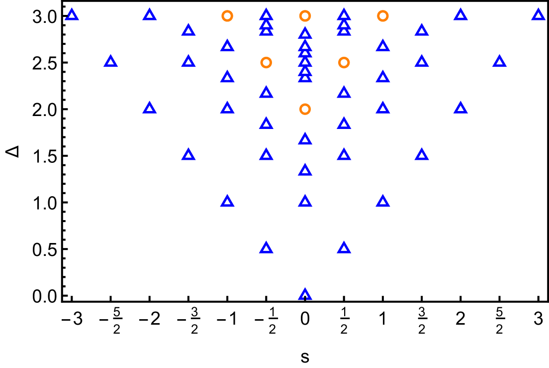
Figure 1: Free conformal dimensions $\Delta=h+\bar{h}$ and spins $s=h-\bar{h}$ of light ($\Delta\leq 3$) states in the symmetric-product orbifold Sym${}_{N}(T^{4})$. We marked sectors with non-trivial mixing under first-order RR-deformation as orange circles. We can observe the relative scarcity in comparison with the states that are corrected only at higher orders in perturbation theory which are denoted by the blue triangles.

As in usual large-$N$ expansions, we define an effective coupling in perturbation theory so that non-planar and perturbative corrections are easily separable. We remember, as discussed in Section 2.2, that a generic genus-g contribution to an $n$-point function in the symmetric-product orbifold has leading $N$ behaviour given by $N^{1-\textrm{g}-n/2}$. Applying this to the planar mixing matrix in consideration here we find $N^{-1/2}$. Then it is useful to define the following effective coupling in perturbation theory

$$\lambda=-\frac{2\pi\xi}{\sqrt{N}}\,,$$ (37)

where $-2\pi$ and $N^{-1/2}$ absorb the factor in (36) and the planar large-$N$ factor, respectively. One can see that $\lambda$ is indeed a good expansion parameter. Consider the $k$-th order in perturbation theory. From (32) we see that this contribution is proportional to

$$\xi^{k}N^{1-\textrm{g}-\frac{(k+2)}{2}}\sim\frac{\lambda^{k}}{N^{\textrm{g}}}\,,$$ (38)

because in the $O(\xi^{k})$ contribution one computes an integrated $(k+2)$-point function. Upon using $\lambda$, the non-planar corrections are suppressed by powers $N^{-\textrm{g}}$, as expected from a ’t Hooft-like expansion.

Let us now introduce an explicit notation for the matrix elements of $\mathcal{M}$, namely

$$_{w\pm 1}\langle Y_{-m_{1}/(w\pm 1)}^{(1)}\cdots Y_{-m_{m^{\prime}}/(w\pm 1)}^{(m^{\prime})}|\mathcal{M}|X_{-n_{1}/w}^{(1)}\cdots X_{-n_{m}/w}^{(m)}\rangle^{xy}_{w}\,,$$ (39)

with $X_{-n_{k}/w}^{(k)}$ and $Y_{-m_{k}/(w\pm 1)}^{(k)}$ representing generic bosonic and/or fermionic excitations detailed in Section 2. Using expressions (36) for the mixing matrix and (37) for the effective coupling we find that a generic mixing matrix element is given by

$$_{w\pm 1}\langle Y_{-m_{1}/(w\pm 1)}^{(1)}\cdots Y_{-m_{m^{\prime}}/(w\pm 1)}^{(m^{\prime})}|\mathcal{M}|X_{-n_{1}/w}^{(1)}\cdots X_{-n_{m}/w}^{(m)}\rangle^{xy}_{w}=\frac{\lambda}{\sqrt{2}}\ C^{\sigma}_{w\pm 1,2,w}\ \times\\ \epsilon_{AB}\epsilon_{\dot{N}\dot{M}}\epsilon_{\dot{Q}\dot{P}}\ {}_{\textrm{NS}}\langle Y_{-m_{1}/(w\pm 1)}^{(1)}\cdots Y_{-m_{m^{\prime}}/(w\pm 1)}^{(m^{\prime})}|(\alpha^{A\dot{Q}}_{-1/2}\tilde{\alpha}^{B\dot{N}}_{-1/2}\mathcal{S}^{\dot{P}\dot{M}})(1)|X_{-n_{1}/w}^{(1)}\cdots X_{-n_{m}/w}^{(m)}\rangle^{xy}_{\textrm{R}}\,.$$ (40)

In the above formula we lifted the correlator on the right-hand side of (36) to the covering surface using the prescription of [35] (and given schematically in (19)). Here $C^{\sigma}_{w\pm 1,2,w}$ denotes the twist field contribution as in (12) (with twists $w$, $w\pm 1$, and $2$). The correlator in the second line of (40) involves free bosons and fermions on the covering surface. The computation of the mixing matrix in each sector $(h,\bar{h},j,\bar{\jmath})$ then reduces to the calculation of these matrix elements. In the next section we show how to compute them.

3.2 Constructing the mixing matrix elements

Here we show the necessary steps to compute the mixing matrix elements of the type (40). The main idea is to break the lifted structure constant on the right-hand side into twist field, boson, and fermion contributions and compute each term independently. We are going to detail how each contribution works in general and also exemplify these using the following matrix element

$$_{2}^{\dot{2}\dot{2}}\langle\alpha_{-1/2}^{1\dot{2}}\tilde{\alpha}_{-1/2}^{2\dot{2}}|\mathcal{M}|\psi^{-\dot{2}}_{-1/2}\psi^{+\dot{2}}_{-1/2}\tilde{\psi}^{\dot{-}\dot{2}}_{-1/2}\tilde{\psi}^{\dot{+}\dot{2}}_{-1/2}\rangle_{1}=\frac{\lambda}{\sqrt{2}}\ C^{\sigma}_{2,2,1}\ \epsilon_{AB}\epsilon_{\dot{N}\dot{M}}\epsilon_{\dot{Q}\dot{P}}\ \mathcal{B}^{A\dot{Q}B\dot{N}}\ \mathcal{F}^{\dot{P}\dot{M}}\,,$$ (41)

where $C^{\sigma}_{2,2,1}$, $\mathcal{B}^{A\dot{Q}B\dot{N}}$, and $\mathcal{F}^{\dot{P}\dot{M}}$ are the twist, bosonic, and fermionic contributions, respectively. Their explicit forms will be given as we compute each one. Note that this is an example of mixing occurring in the sector $(1,1,0,0)$ described in Table 3.

The last ingredient we need is the covering map used to lift the mixing matrix element computations to the covering surface and also to define the bosonic and fermionic modes in (17) and (18), which are

$$\mathbf{\Gamma}_{+}(t)=(w+1)t^{w}-wt^{w+1}\,,\qquad\mathbf{\Gamma}_{-}(t)=\frac{t^{w}}{wt-w+1}\,,$$ (42)

for $w$-$(w+1)$ and $w$-$(w-1)$ mixings, respectively. It can be checked that these follow the expansion (13) around the insertion points as expected.

3.2.1 Twist field contribution

The twist field contribution amounts to computing the three-point function of normalised twist operators and it was found in [34]. We write this result below as

$$C^{\sigma}_{n,m,q}=\sqrt{nmq}\ |\mathcal{C}_{nmq}|^{\mathbf{c}}\,,$$ (43)

where $\mathbf{c}$ is the central charge of the seed theory and $n$, $m$, and $q$ are the twists of the operator insertions. The $|\mathcal{C}_{nmq}|$ is given by the following rather unwieldy expression

$$\log|\mathcal{C}_{nmq}|^{2}=\frac{1}{6}\log\left(\frac{q}{nm}\right)-\frac{n-1}{12}\log n-\frac{m-1}{12}\log m+\frac{q-1}{12}\log q\\ -\frac{n-1}{12n}\log\left(\frac{d_{1}!d_{2}!}{n!(n-1)!}\frac{(d_{1}-m)!}{(d_{1}-n)!}\right)-\frac{m-1}{12m}\log\left(\frac{d_{1}!d_{2}!}{m!(m-1)!}\frac{(d_{1}-n)!}{(d_{1}-m)!}\right)\\ +\frac{q-1}{12q}\log\left(\frac{(q-1)!d_{2}!}{(d_{1}-n)!(d_{1}-m)!}\frac{(d_{1}-d_{2})!}{d_{1}!}\right)+\frac{d_{2}(d_{2}-1)}{3}\log 2-\frac{d_{2}}{6}\log n+\frac{\log\mathcal{D}}{3}\\ +\frac{(3d_{2}-4)}{6}\log d_{2}!-\frac{d_{2}}{6}\log\left(\frac{d_{1}!}{n!(d_{1}-n)!}\right)-\frac{(n+d_{2}-1)}{6}\log\left(\frac{(n-1)!}{(n-d_{2}-1)!}\right)\\ -\frac{(d_{1}-d_{2}+3)}{6}\log\left(\frac{(d_{1}-d_{2})!}{d_{1}!}\right)-\frac{(d_{1}+d_{2}-n)}{6}\log\left(\frac{(d_{1}+d_{2}-n)!}{(d_{1}-n)!}\right)\,,$$ (44)

with $d_{1}$, $d_{2}$, and $\mathcal{D}$ being

$$d_{1}=\frac{n+m+q-1}{2}\,,$$ (45)

$$d_{2}=\frac{n+m-q-1}{2}\,,$$ (46)

$$\mathcal{D}=\frac{1}{2^{d_{2}(d_{2}-1)}}\prod_{k=1}^{d_{2}}k^{k+2-2d_{2}}(k-n)^{k-1}(k-d_{1}-d_{2}+n-1)^{k-1}(k-d_{1}-1)^{d_{2}-k}\ .$$ (47)

Note that this expression is universal and is dependent on the seed theory only through the central charge $\mathbf{c}$. Although it is not manifest, this expression is fully symmetric in $n$, $m$, and $q$.

For the mixing matrix applications, we are interested in the case with $\mathbf{c}=6$ (see Appendix A) and fixed twists. We then only need the expressions

$$C^{\sigma}_{w+1,2,w}=\frac{w^{-\frac{w(2w+3)+3}{8(w+1)}}(w+1)^{\frac{2w^{2}+w+2}{8w}}}{2^{5/8}}\,,\qquad C^{\sigma}_{w-1,2,w}=\frac{(w-1)^{\frac{-2w^{2}+w-2}{8w}}w^{\frac{2w^{2}-3w+3}{8(w-1)}}}{2^{5/8}}\,.$$ (48)

For the example (41) the twist contribution is simply

$$C^{\sigma}_{2,2,1}=1\,,$$ (49)

which is expected since the twist operators are unit normalised and in this case the structure constant reduces to the norm of the two-point function of twist-2 operators.

3.2.2 Boson contribution

This contribution involves only the bosonic modes $\alpha^{A\dot{A}}_{-n/w}$ and $\tilde{\alpha}^{A\dot{A}}_{-n/w}$ of the excited states in the mixing matrix elements. To compute it we first convert the modes into fields by using their definition (17) and end up with an integrated free boson correlator. This correlator is computed by usual Wick contractions. However, due to the factorisation of Wick contractions we may equally factorise the integrals and compute them contraction-by-contraction. Using this we can analytically compute all Wick contractions involving bosonic modes around $0$ (right state in (40)), around $1$ (deformation mode), and around $\infty$ (left state in (40)). For instance, an integrated Wick contraction involving bosonic modes of the left and right states is given generically by

$$\wick{(\c{1}\alpha^{B\dot{B}}_{m/(w\pm 1)})_{\infty}(\c{1}\alpha^{A\dot{A}}_{-n/w})_{0}}=\frac{-\epsilon^{AB}\epsilon^{\dot{A}\dot{B}}}{\sqrt{w(w\pm 1)}}\oint_{\infty}\frac{dt^{\prime}}{2\pi i}\oint_{0}\frac{dt}{2\pi i}\ \mathbf{\Gamma}_{\pm}(t^{\prime})^{m/(w\pm 1)}\mathbf{\Gamma}_{\pm}(t)^{-n/w}\frac{1}{(t-t^{\prime})^{2}}\,,$$ (50)

for a mixing involving twists $w$ and $w\pm 1$. Similar expressions can be found for integrated Wick contractions involving all other modes. Note that the $SU(2)_{\circ}$ and $SU(2)_{\bullet}$ indices are simply contracted with the $SU(2)$-invariant structure $\epsilon$ and the integrated Wick contractions can thus be written as

$$\wick{(\c{1}\alpha^{B\dot{B}}_{-m/w})_{0}(\c{1}\alpha^{A\dot{A}}_{-n/w})_{0}}=\epsilon^{AB}\epsilon^{\dot{A}\dot{B}}\ \mathcal{W}_{00}^{\pm}(n,m)\,,$$ (51)

$$\wick{(\c{1}\alpha^{B\dot{B}}_{-1/2})_{1}(\c{1}\alpha^{A\dot{A}}_{-n/w})_{0}}=\epsilon^{AB}\epsilon^{\dot{A}\dot{B}}\ \mathcal{W}_{01}^{\pm}(n)\,,$$ (52)

$$\wick{(\c{1}\alpha^{B\dot{B}}_{m/(w\pm 1)})_{\infty}(\c{1}\alpha^{A\dot{A}}_{-n/w})_{0}}=\epsilon^{AB}\epsilon^{\dot{A}\dot{B}}\ \mathcal{W}_{0\infty}^{\pm}(n,m)\,,$$ (53)

$$\wick{(\c{1}\alpha^{B\dot{B}}_{m/(w\pm 1)})_{\infty}(\c{1}\alpha^{A\dot{A}}_{-1/2})_{1}}=\epsilon^{AB}\epsilon^{\dot{A}\dot{B}}\ \mathcal{W}_{1\infty}^{\pm}(m)\,,$$ (54)

$$\wick{(\c{1}\alpha^{B\dot{B}}_{m/(w\pm 1)})_{\infty}(\c{1}\alpha^{A\dot{A}}_{n/(w\pm 1)})_{\infty}}=\epsilon^{AB}\epsilon^{\dot{A}\dot{B}}\ \mathcal{W}_{\infty\infty}^{\pm}(n,m)\,,$$ (55)

with similar expressions for the right-moving modes. The right-hand side factors correspond to integrals similar to (50), which can be computed analytically and are given in Appendix D.

With these tools we can compute the bosonic contribution in our example (41). It is explicitly given by

$$\mathcal{B}^{A\dot{Q}B\dot{N}}=-\langle 0|(\alpha_{1/2}^{2\dot{1}}\tilde{\alpha}_{1/2}^{1\dot{1}})_{\infty}(\alpha^{A\dot{Q}}_{-1/2}\tilde{\alpha}^{B\dot{N}}_{-1/2})_{1}|0\rangle\,,$$ (56)

where the modes are grouped by the point (indicated in the subscript $\infty$ and $1$ in this example) around which we integrate the boson fields using the definition (17). Note that we have a minus sign coming from conjugation of the modes in the state using the conjugation rule (A.9). As described before, we could write explicitly the integrated boson correlator, compute the integrand using Wick contractions and then integrate the latter. However, by using the previously described factorisation of Wick contractions and relation (54) we find

$$\mathcal{B}^{A\dot{Q}B\dot{N}}=\frac{1}{2}\ \delta^{A}_{1}\delta^{B}_{2}\delta^{\dot{Q}}_{\dot{2}}\delta^{\dot{N}}_{\dot{2}}\ ,$$ (57)

which completes the computation of the bosonic contribution to (41).

3.2.3 Fermion contribution and bosonisation

The fermion contribution is computed analogously to the bosonic term. That is, we write the fermionic modes using (18) and then we calculate integrated fermionic correlators. To compute these fermion correlators we are going to use bosonisation, which is useful when spin fields are present. For this we introduce left- and right-moving bosons $\phi_{a}(t)$ and $\tilde{\phi}_{a}(\bar{t})$ with $a=1,2$. The fermions and spin fields are then given by

$$\begin{gathered}\psi^{\alpha\dot{A}}(t)=C^{\alpha\dot{A}}:e^{i\boldsymbol{q}^{\alpha\dot{A}}\cdot\phi(t)}:\,,\qquad\tilde{\psi}^{\dot{\alpha}\dot{A}}(\bar{t})=\tilde{C}^{\dot{\alpha}\dot{A}}:e^{i\boldsymbol{q}^{\dot{\alpha}\dot{A}}\cdot\tilde{\phi}(\bar{t})}:\,,\\ \mathcal{S}^{xy}(t,\bar{t})=Q^{xy}:e^{i\boldsymbol{\xi}^{x}\cdot\phi(t)}e^{i\boldsymbol{\xi}^{y}\cdot\tilde{\phi}(\bar{t})}:\,,\end{gathered}$$ (58)

with the prefactors $C^{\alpha\dot{A}}$, $\tilde{C}^{\dot{\alpha}\dot{A}}$, and $Q^{xy}$ being cocycles which ensure the correct statistics of the fields. The definition of $\boldsymbol{q}^{\alpha\dot{A}}$, $\boldsymbol{q}^{\dot{\alpha}\dot{A}}$, and $\boldsymbol{\xi}^{x}$ and a detailed description of the bosonisation procedure used here are reported in Appendix E. The main point of introducing bosonisation is that the fermion correlators boil down to vertex-operator correlators which are known to evaluate to [52]

$$\langle:e^{i\boldsymbol{\xi}_{1}\cdot\phi(t_{1})}:\cdots:e^{i\boldsymbol{\xi}_{n}\cdot\phi(t_{n})}:\rangle=\prod_{i<j}t_{ji}^{\boldsymbol{\xi}_{i}\cdot\boldsymbol{\xi}_{j}}\ \ \ \textrm{with}\ \ \ \sum_{i}\boldsymbol{\xi}_{i}=0\ ,$$ (59)

where radial ordering ($|t_{j+1}|>|t_{j}|$) is assumed. For right-moving operators we have a similar contribution. The vanishing of the sum over all polarisations is just the statement of charge neutrality of the correlator.

We now compute the fermionic contribution of our example mixing matrix element (41). First we note that by combining the index structure of (41) with the one coming from the bosonic contribution (57) we can fix the indices of the fermionic contribution. It is given as

$$\mathcal{F}^{\dot{P}\dot{M}}=\delta_{\dot{1}}^{\dot{P}}\delta_{\dot{1}}^{\dot{M}}\ {}_{\textrm{NS}}\langle 0|(\mathcal{S}^{\dot{1}\dot{1}})_{\infty}(\mathcal{S}^{\dot{1}\dot{1}})_{1}(\psi^{-\dot{2}}_{-1/2}\psi^{+\dot{2}}_{-1/2}\tilde{\psi}^{\dot{-}\dot{2}}_{-1/2}\tilde{\psi}^{\dot{+}\dot{2}}_{-1/2})_{0}|0\rangle_{\textrm{NS}}\,,$$ (60)

where the conjugation rules like (A.10) were used. By using the mode definition (18) it is possible to rewrite it as

$$\mathcal{F}^{\dot{P}\dot{M}}=\delta_{\dot{1}}^{\dot{P}}\delta_{\dot{1}}^{\dot{M}}\oint_{0}\frac{dt_{1}}{2\pi i}\oint_{0}\frac{dt_{2}}{2\pi i}\oint_{0}\frac{d\bar{t}_{1}}{2\pi i}\oint_{0}\frac{d\bar{t}_{2}}{2\pi i}\ \frac{(\partial\mathbf{\Gamma}_{+}(t_{1}))^{1/2}}{\mathbf{\Gamma}_{+}(t_{1})}\frac{(\partial\mathbf{\Gamma}_{+}(t_{2}))^{1/2}}{\mathbf{\Gamma}_{+}(t_{2})}\frac{(\partial\mathbf{\Gamma}_{+}(\bar{t}_{1}))^{1/2}}{\mathbf{\Gamma}_{+}(\bar{t}_{1})}\times\\ \frac{(\partial\mathbf{\Gamma}_{+}(\bar{t}_{2}))^{1/2}}{\mathbf{\Gamma}_{+}(\bar{t}_{2})}\ _{\textrm{NS}}\langle 0|\mathcal{S}^{\dot{1}\dot{1}}(\infty)\mathcal{S}^{\dot{1}\dot{1}}(1)\psi^{-\dot{2}}(t_{1})\psi^{+\dot{2}}(t_{2})\tilde{\psi}^{\dot{-}\dot{2}}(\bar{t}_{1})\tilde{\psi}^{\dot{+}\dot{2}}(\bar{t}_{2})|0\rangle_{\textrm{NS}}\,.$$ (61)

The correlator in the integrand is found by using the bosonisation prescription (see Appendix E) combined with formula (59). In this particular case it is simply

$${}_{\textrm{NS}}\langle 0|\mathcal{S}^{\dot{1}\dot{1}}(\infty)\mathcal{S}^{\dot{1}\dot{1}}(1)\psi^{-\dot{2}}(t_{1})\psi^{+\dot{2}}(t_{2})\tilde{\psi}^{\dot{-}\dot{2}}(\bar{t}_{1})\tilde{\psi}^{\dot{+}\dot{2}}(\bar{t}_{2})|0\rangle_{\textrm{NS}}=\\ (1-t_{1})^{-1/2}(1-t_{2})^{-1/2}(1-\bar{t}_{1})^{-1/2}(1-\bar{t}_{2})^{-1/2}.$$ (62)

Integrating the above result as in (61) we find the following fermionic contribution

$$\mathcal{F}^{\dot{P}\dot{M}}=\frac{1}{4}\ \delta_{\dot{1}}^{\dot{P}}\delta_{\dot{1}}^{\dot{M}}\,.$$ (63)

Finally, combining the twist field (49), the bosonic (57), and the fermionic (63) contributions with expression (41) we can construct the desired matrix element

$$_{2}^{\dot{2}\dot{2}}\langle\alpha_{-1/2}^{1\dot{2}}\tilde{\alpha}_{-1/2}^{2\dot{2}}|\mathcal{M}|\psi^{-\dot{2}}_{-1/2}\psi^{+\dot{2}}_{-1/2}\tilde{\psi}^{\dot{-}\dot{2}}_{-1/2}\tilde{\psi}^{\dot{+}\dot{2}}_{-1/2}\rangle_{1}=\frac{\lambda}{4\sqrt{2}}\,.$$ (64)

We remark that expression (40) for generic mixing matrix elements is valid for normalised states, thus (64) is found after dividing by the norms of the left and right states in (41).

3.3 Anomalous dimensions for light states

Having established the necessary techniques to compute mixing matrices, we now move on to the analysis of low-lying states with bare dimension $\Delta\leq 3$. As exemplified in Table 3 the number of such states in each mixing sector is large and so we automated the mixing matrix computation in Wolfram Mathematica. The interested reader can consult the ancillary file in the arXiv submission.

As discussed above, the mixing problem can be broken down into sectors labelled by conformal dimensions and R-charges $(h,\bar{h},j,\bar{\jmath})$, which remain independent under first-order RR-deformation. However these are not the only restrictions to mixing. Indeed, due to the bosonic contribution, detailed in Section 3.2.2, we observe that non-vanishing mixing only occurs when the overall number of bosonic excitations in in- and out-state is odd in both left-moving and right-moving sector. This is such that one can absorb the bosonic modes of the deformation seen in eq. (40). One immediate consequence of this is that half-BPS operators are not corrected, as expected (see Appendix C). Combining this restriction on bosonic oscillators with the fact that mixing occurs only between twist $w$ and $w\pm 1$ sectors we see that numerous sectors are excluded, such as those with $h,\bar{h}\notin\mathbb{Z}/2$ as illustrated in Figure 1.

With all these restrictions we are left with 15 non-trivial sectors for bare dimension $\Delta\leq 3$ which fit into five groups

$$\begin{split}\text{Group 1:}&\quad(1,1,0,0)\,,\\ \text{Group 2:}&\quad(1,\tfrac{3}{2},0,\tfrac{1}{2})\,,\quad(1,\tfrac{3}{2},0,-\tfrac{1}{2})\,,\quad(\tfrac{3}{2},1,\tfrac{1}{2},0)\,,\quad(\tfrac{3}{2},1,-\tfrac{1}{2},0)\,,\\ \text{Group 3:}&\quad(1,2,0,1)\,,\quad(1,2,0,-1)\,,\quad(2,1,1,0)\,,\quad(2,1,-1,0)\,,\\ \text{Group 4:}&\quad(\tfrac{3}{2},\tfrac{3}{2},\tfrac{1}{2},\tfrac{1}{2})\,,\quad(\tfrac{3}{2},\tfrac{3}{2},\tfrac{1}{2},-\tfrac{1}{2})\,,\quad(\tfrac{3}{2},\tfrac{3}{2},-\tfrac{1}{2},\tfrac{1}{2})\,,\quad(\tfrac{3}{2},\tfrac{3}{2},-\tfrac{1}{2},-\tfrac{1}{2})\,,\\ \text{Group 5:}&\quad(1,2,0,0)\,,\quad(2,1,0,0)\,.\end{split}$$ (65)

The sectors within each group are related by exchanging left- and right-moving fields or inverting the R-charge and thus have the same spectrum of anomalous dimensions. It is therefore enough to compute the mixing matrix in the first sector of each group.

One could further decompose each sector in irreducible representations of $SU(2)_{\bullet}\times SU(2)_{\circ}$ which mix strictly among themselves. However, this was not necessary for our purposes where the full mixing matrix could already be generated in a reasonable amount of time. We simply determined the $SU(2)_{\bullet}\times SU(2)_{\circ}$ representations retrospectively to verify that mixing does not occur between different irreducible representations.

For the lowest sector $(1,1,0,0)$ we found that 74 of the 276 states are mixed by the RR-deformation and acquire an anomalous dimension. We present the results of the diagonalisation of the mixing matrix in Table 4. Although the eigenvalues can be computed analytically, they do not follow any obvious pattern apart from appearing in pairs of opposite sign. We also presented which untwisted states partake in mixing. For example, one eigenstate in the first eigenspace of Table 4 is approximately given by the combination

$$(0.3-0.5i)\big{|}\psi_{-\frac{1}{2}}^{+\dot{1}}\psi_{-\frac{1}{2}}^{-\dot{1}}\tilde{\psi}_{-\frac{1}{2}}^{+\dot{1}}\tilde{\psi}_{-\frac{1}{2}}^{-\dot{1}}\big{\rangle}_{1}+(0.3-0.4i)\epsilon_{AB}\big{|}\alpha_{-\frac{1}{2}}^{A\dot{1}}\tilde{\alpha}_{-\frac{1}{2}}^{B\dot{1}}\big{\rangle}_{2}^{\dot{1}\dot{1}}+0.4\big{|}\psi_{-\frac{1}{2}}^{+\dot{1}}\psi_{-\frac{1}{2}}^{-\dot{1}}\tilde{\psi}_{-\frac{1}{6}}^{+\dot{1}}\tilde{\psi}_{-\frac{1}{6}}^{-\dot{1}}\big{\rangle}_{3}\,.$$ (66)

It can also be seen that the eigenstates organise themselves in irreducible representations of $SU(2)_{\bullet}\times SU(2)_{\circ}$ (see Table 5) so the index structure of the constituents is necessarily aligned. Note that the sector $(1,1,0,0)$ contains the RR-deformation operator (31) itself, but our analysis shows that it does not participate in first order mixing (i.e. it is part of “all other states" in Table 4). This is an important consistency check because it tell us that the deformation considered remains exactly marginal at first order in perturbation theory.

$\gamma/\lambda$	Numerical values	# states	Constituent states
$\pm\frac{1}{12}\sqrt{9+2^{\frac{8}{3}}3^{-\frac{1}{2}}}$	$\pm 0.2966$	9	$\big{|}\psi_{-\frac{1}{2}}^{+(\dot{A}}\psi_{-\frac{1}{2}}^{-\dot{B})}\tilde{\psi}_{-\frac{1}{2}}^{+(\dot{C}}\tilde{\psi}_{-\frac{1}{2}}^{-\dot{D})}\big{\rangle}_{1}$ $\epsilon_{AB}\big{|}\alpha_{-\frac{1}{2}}^{A(\dot{A}}\tilde{\alpha}_{-\frac{1}{2}}^{B(\dot{C}}\big{\rangle}_{2}^{\dot{B})\dot{D})}$ $\big{|}\psi_{-\frac{1}{2}}^{+(\dot{A}}\psi_{-\frac{1}{2}}^{-\dot{B})}\tilde{\psi}_{-\frac{1}{6}}^{+(\dot{C}}\tilde{\psi}_{-\frac{1}{6}}^{-\dot{D})}\big{\rangle}_{3}$
$\pm 2^{-\frac{25}{24}}3^{-\frac{55}{16}}\sqrt{27+2^{\frac{27}{4}}3^{\frac{3}{8}}}$	$\pm 0.1532$	4	$\epsilon_{\pm\mp}{\epsilon}_{\dot{\pm}\dot{\mp}}\big{|}\psi_{-\frac{1}{2}}^{\pm\dot{A}}\tilde{\psi}_{-\frac{1}{2}}^{\pm^{\prime}\dot{B}}\big{\rangle}_{2}^{\mp\dot{\mp}}$ $\epsilon_{AB}\big{|}\alpha_{-\frac{1}{3}}^{A\dot{A}}\tilde{\alpha}_{-\frac{1}{3}}^{B\dot{B}}\big{\rangle}_{3}$ $|0\rangle_{4}^{\dot{A}\dot{B}}$
$\pm 2^{\frac{1}{3}}3^{-\frac{9}{4}}$	$\pm 0.1064$	24 (12+12)	$\epsilon_{\pm\mp}\big{|}\psi_{-\frac{1}{2}}^{\pm\dot{A}}\tilde{\alpha}_{-\frac{1}{2}}^{A(\dot{B}}\big{\rangle}_{2}^{\mp\dot{C})}$ $\big{|}\alpha_{-\frac{1}{3}}^{A\dot{A}}\tilde{\psi}_{-\frac{1}{2}}^{+(\dot{B}}\tilde{\psi}_{-\frac{1}{2}}^{-\dot{C})}\big{\rangle}_{3}$ $\epsilon_{\pm\mp}\big{|}\alpha_{-\frac{1}{2}}^{A(\dot{B}}\tilde{\psi}_{-\frac{1}{2}}^{\pm\dot{A}}\rangle_{2}^{\dot{C})\mp}$ $\big{|}\psi_{-\frac{1}{2}}^{+(\dot{B}}\psi_{-\frac{1}{2}}^{-\dot{C})}\tilde{\alpha}_{-\frac{1}{3}}^{A\dot{A}}\big{\rangle}_{3}$
$0$	$0$	202	All other states

Table 4: Anomalous dimensions $\gamma$ and constituent fields in sector $(1,1,0,0)$. The parentheses in the index structure denote symmetrisation and it only affects the two indices right next to them. In the third row we observe two closed degenerate subsectors related by left-right symmetry.

The following sectors in (65) have a growing number of distinct eigenvalues. Crucially, the anomalous dimensions found in sector $(1,1,0,0)$ reappear. This is expected since the RR-deformation does not break the superconformal symmetry of the theory. As a result the deformed states in $(1,1,0,0)$ generate long superconformal multiplets, such that their descendants will reappear in other sectors and have the same anomalous dimension. We demonstrate this effect by listing the anomalous dimensions and $SU(2)_{\bullet}\times SU(2)_{\circ}$-representations of the sectors $(1,1,0,0)$ and $(1,\tfrac{3}{2},0,\tfrac{1}{2})$ in Table 5. Acting with the supercharges $\tilde{G}_{-1/2}^{\dot{+}A}$ (defined in (B.10)) on states in sector $(1,1,0,0)$ will generate an $SU(2)_{\bullet}$-doublet of states in sector $(1,\tfrac{3}{2},0,\tfrac{1}{2})$. We find precisely these states in an explicit diagonalisation.

Sector	$\gamma/\lambda$	# states	$SU(2)_{\bullet}\crossproduct SU(2)_{\circ}$ representation
$(1,1,0,0)$	$\pm 0.2966$	9	$(0,2)\oplus(0,1)\oplus(0,0)$
	$\pm 0.1532$	4	$(0,1)\oplus(0,0)$
	$\pm 0.1064$	24	$2\crossproduct\left[(\frac{1}{2},\frac{3}{2})\oplus(\frac{1}{2},\frac{1}{2})\right]$
	$0$	202	Various representations
$(1,\tfrac{3}{2},0,\pm\tfrac{1}{2})$ and $(\tfrac{3}{2},1,\pm\tfrac{1}{2},0)$	$\mathbf{\underline{\pm 0.2966}}$	18	$(\tfrac{1}{2},2)\oplus(\tfrac{1}{2},1)\oplus(\tfrac{1}{2},0)$
	$\pm 0.2568$	6	$(0,\tfrac{3}{2})\oplus(0,\tfrac{1}{2})$
	$\pm 0.1876$	18	$(\tfrac{1}{2},2)\oplus(\tfrac{1}{2},1)\oplus(\tfrac{1}{2},0)$
	$\mathbf{\underline{\pm 0.1532}}$	8	$(\tfrac{1}{2},1)\oplus(\tfrac{1}{2},0)$
	$\pm 0.1398$	6	$(0,\tfrac{3}{2})\oplus(0,\tfrac{1}{2})$
	$\pm 0.1303$	54	$(1,\tfrac{5}{2})\oplus(1,\tfrac{3}{2})\oplus(1,\tfrac{1}{2})\oplus(\tfrac{1}{2},1)\oplus(0,\tfrac{5}{2})\oplus(0,\tfrac{3}{2})\oplus(0,\tfrac{1}{2})$
	$\pm 0.1251$	2	$(0,\tfrac{1}{2})$
	$\mathbf{\underline{\pm 0.1064}}$	48	$2\crossproduct\left[(1,\tfrac{3}{2})\oplus(1,\tfrac{1}{2})\oplus(0,\tfrac{3}{2})\oplus(0,\tfrac{1}{2})\right]$
	$\pm 0.0971$	18	$(2,\tfrac{1}{2})\oplus(1,\tfrac{1}{2})\oplus(0,\tfrac{1}{2})$
	$\pm 0.0921$	8	$(\tfrac{1}{2},1)\oplus(\tfrac{1}{2},0)$
	$\pm 0.0869$	6	$(\tfrac{1}{2},1)$
	$\pm 0.0485$	24	$(1,\tfrac{3}{2})\oplus(1,\tfrac{1}{2})\oplus(0,\tfrac{3}{2})\oplus(0,\tfrac{1}{2})$
	$\pm 0.0483$	8	$(\tfrac{1}{2},1)\oplus(\tfrac{1}{2},0)$
	$\pm 0.0357$	8	$(\tfrac{1}{2},1)\oplus(\tfrac{1}{2},0)$
	$0$	626	Various representations

Table 5: Anomalous dimensions $\gamma$ and $SU(2)_{\bullet}\crossproduct SU(2)_{\circ}$ representations of states in the lightest non-trivial sectors. The highlighted states are descendants from the $(1,1,0,0)$ sector. Note that their representation is the tensor product of the $(1,1,0,0)$ states with an additional $SU(2)_{\bullet}$-doublet.

We present the full spectrum of the five distinct groups (65) in Figure 2. For simplicity we are not going to show all the numerical value of the eigenvalues in a table, however we give them in the ancillary file in the arXiv submission. The numbers of perturbed states are presented in Table 6. We note that a fraction of 12.4% of physical states with bare dimension $\Delta\leq 3$ receive first-order corrections. We expect this fraction to decrease as $\Delta=h+\bar{h}$ increases — the size of the mixing sectors grows with $\Delta$, but parametrically slower than the size of the Fock subspace with given $\Delta$ (see Figure 1). Nonetheless, infinitely many such $O(\lambda)$ mixing sectors appear as $\Delta$ grows.

group	$\Delta$	# states	# deformed states	fraction
1	2	$276$	$74$	26.8%
2	$\frac{5}{2}$	$4\times 1090$	$4\times 464$	42.6%
3	3	$4\times 2368$	$4\times 1210$	51.1%
4	3	$4\times 6467$	$4\times 3828$	59.2%
5	3	$2\times 8280$	$2\times 4342$	52.4%
All	$\leq 3$	$248778$	$30766$	12.4%

Table 6: Numbers of total and deformed states in sectors grouped as in (65). We also give the total number of physical states that do (or do not) receive corrections at order $O(\lambda)$ with bare dimension $\Delta\leq 3$.

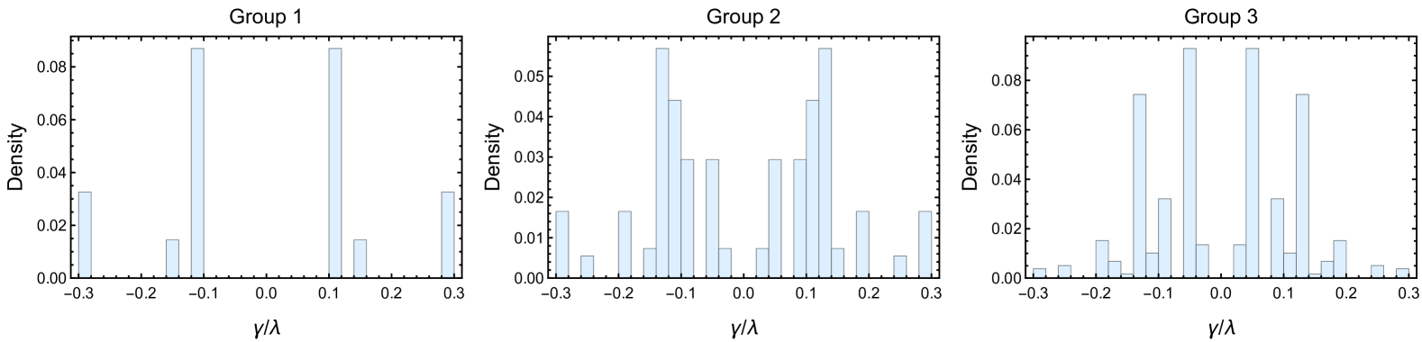
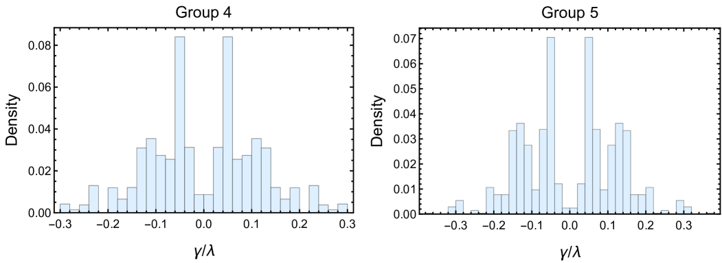
Figure 2: Density of non-vanishing eigenvalues of the mixing matrix, for each of the five groups of states listed in (65).

4 Relation to integrability

The integrability approach to AdS3/CFT2 is most easily explained by starting from the worldsheet of the type IIB string on $AdS_{3}\times S^{3}\times T^{4}$ background, where it was first developed (see [12, 13, 14] for reviews). By fixing a suitable lightcone gauge along coordinates $X^{\pm}$ (whereby the density of the conjugate momentum $P_{-}$ is constant), one obtains a non-conformal QFT in two dimensions, whose fields are the transverse excitations of a string of finite length $R$. If the choice of the gauge fixing condition preserves as much supersymmetry as possible (half, in this case), the length can be identified with the charge of a half-BPS state $|\text{BPS}\rangle_{R}$. Integrability is manifest in the $R\to\infty$ limit of the theory, whereby the worldsheet decompactifies to a plane and one can construct a factorised S-matrix. The two-to-two scattering matrix $S(p_{1},p_{2})$ is bootstrapped from the symmetries, with the exception of an overall scalar pre-factor (the “dressing factor”) for which one can make an Ansatz based on unitarity, crossing symmetry, analyticity, and comparison with perturbative computations [53, 54, 55, 56].

On the orbifold side of the duality, it is natural to identify $|\text{BPS}\rangle_{R}$ with one of the half-BPS states in Appendix C, constructed out of the $w$-cycle sector of the model with $w=R$. Hence, it is expected that integrability arises in the $w\to\infty$ limit. By representation theory it is clear that the transverse fields of the strings in lightcone gauge must be identified with the fields of the orbifold [19], and more specifically that worldsheet excitations (i.e., particles of momentum $p$) above the lightcone vacuum must be identified with the creation operators on the $w$-cycle “vacuum” (with fractional mode $n/w$).

It is therefore natural to explore the $w\to\infty$ limit of the $O(\lambda)$ mixing matrix and see how its behaviour fits in the integrability picture. This will also give us an opportunity to revisit some of the arguments of [18] and point out some important issues that must be addressed to link the orbifold model to the integrability structure. Finally, a more difficult (but crucial) question is what integrability predicts at finite $w$ and $O(\lambda)$, and whether this is compatible with our results.

4.1 Order-$\lambda$ mixing matrix in the $w\to\infty$ limit

Since the dimensions of the twist vacuum (20–21) increase with $w$, the large-$w$ limit requires the bare dimension $\Delta$ to be large; in turn, this implies dealing with a very large mixing problem, making explicit computations along the lines of Section 3.3 unfeasible. Of course while the number of states which may mix at $O(\lambda)$ grows, the total number of states grows even faster, see Figure 1.

Let us now consider the large-$w$ behaviour of a generic mixing matrix element of the type (40). The most straightforward part is the twist-field structure function $C_{w\pm 1,2,w}^{\sigma}$ which behaves as

$$\lim_{w\to\infty}C_{w\pm 1,2,w}=e^{1/4}2^{-5/8}\,.$$ (67)

Consider now the boson contributions of Section 3.2.2. In this case it is useful to work in terms of “momenta” $p_{j}=n_{j}/w$, rather than mode numbers $n_{j}$; this will allow us to consider the scaling limit where $w\to\infty$ with $p_{j}$ fixed, which is natural in integrability (and more generally, at large-$w$). The commutation relation (27) suggests that the normalisation of the bosonic oscillators requires the introduction of factors $1/\sqrt{\absolutevalue{p}}$ which are generically finite in the large-$w$ limit. With this normalisation we can compute the limit of the bosonic Wick contractions (51)-(55). To do so we use the building blocks $\mathcal{V}_{w}(n)$ and $\mathcal{V}_{-(w+1)}(m)$ defined in (D.9) in Appendix D so that the Wick contractions are given by (D.10–D.19). Without loss of generality we focus on $w$ and $w+1$ mixing. By assuming unit-normalised bosonic oscillators we can write these blocks as a function of the momentum as:

$$\mathcal{V}_{w}(p)=\sqrt{\frac{2}{\absolutevalue{(w+1)p}}}\left(\frac{w}{w+1}\right)^{p(w+1)-1}w^{-p}\frac{\Gamma(p(w+1))}{\Gamma(pw)\Gamma(p)}\,,$$ (68)

with a similar expression for $\mathcal{V}_{-(w+1)}(q)$ where $q=m/(w+1)$. By making use of the following elementary limits

$$\lim_{w\to\infty}\left(\frac{w}{w+1}\right)^{p(w+1)}=e^{-p}\,,\qquad\lim_{w\to\infty}w^{-p}\frac{\Gamma(p(w+1))}{\Gamma(pw)}=p^{p}\,,$$ (69)

one then finds the following asymptotic behaviour for the Wick contraction building blocks:

$$\mathcal{V}_{w}(n)\ \rightarrow\ \frac{1}{\sqrt{w}}\,\mathcal{V}_{\infty}(p)\,,\qquad\mathcal{V}_{-(w+1)}(m)\ \rightarrow\ \frac{1}{\sqrt{w}}\,{\mathcal{V}}_{\infty}(-q)\,,$$ (70)

where

$$\mathcal{V}_{\infty}(p)=\sqrt{\frac{2}{\absolutevalue{p}}}\frac{e^{-p}p^{p}}{\Gamma(p)}\,.$$ (71)

We can see in Figure 3 that the asymptotic function $\mathcal{V}_{\infty}$ is a good approximation of the finite result already for $w=10$.

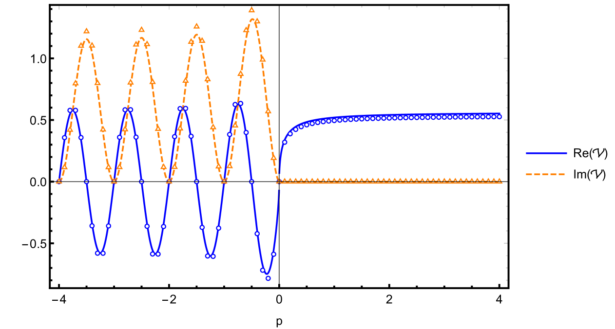
Figure 3: The asymptotic function $\mathcal{V}_{\infty}(p)$ as well as the $w=10$ real (circles) and imaginary parts (triangles) of appropriately rescaled $\mathcal{V}_{w}(n)$, respectively. We notice a good approximation already at relatively small twist $w$. The zeros at negative integer values are needed to cancel the poles in the propagator.

The final ingredients which we need are the “propagators” appearing in Wick-contractions among in- and out-state excitations (D.10),(D.12),(D.14). While contractions of two in-state or two out-state excitations among themselves only result in a finite factor, a contraction of one in- and one out-state excitation results in a contribution like

$$\frac{1}{2}\frac{1}{\frac{n}{w}-\frac{m}{w+1}}\qquad\rightarrow\qquad\frac{1}{2}\frac{1}{p-q}\,,$$ (72)

which generates a pole at coinciding incoming and outgoing momenta. At finite $w$ these momenta are fractions with co-prime denominators, so they can only truly coincide at integer values of $p$ and $q$; in this case however, the accompanying factor of $\mathcal{V}_{\infty}(-q)$ vanishes and cancels the pole (see fig.3). At large $w$ however, non-coincident values can get parametrically close, e.g.

$$p=\frac{n}{w}\,,\quad q=\frac{n}{w+1}\,:\qquad\frac{1}{p-q}=\frac{1}{\frac{n}{w}-\frac{n}{w+1}}=\frac{w(w+1)}{n}=\frac{w}{q}\,,$$ (73)

generating a resonance that contributes with another (large) factor $w$.

Let us now discuss which $O(\lambda)$-processes are least suppressed at large-$w$. We start with states involving only two bosonic excitations. Schematically the boson contribution to three-point functions on the right-hand side of (40) behaves as

$$\begin{gathered}{}_{w+1}\bra{0\phantom{{}_{j}}\hskip-2.0pt}\mathcal{D}\ket{\alpha_{-p}\tilde{\alpha}_{-\bar{p}}}_{w}=O(w^{-1})\,,\qquad_{w+1}\bra{\alpha_{-q}\tilde{\alpha}_{-\bar{q}}}\mathcal{D}\ket{\,0\phantom{{}_{j}}\hskip-3.0pt}_{w}=O(w^{-1})\,,\\ {}_{w+1}\bra{\alpha_{-q}}\mathcal{D}\ket{\tilde{\alpha}_{-\bar{p}}}_{w}=O(w^{-1})\,,\end{gathered}$$ (74)

for finite momenta $p,\bar{p},q,\bar{q}$. In this case both bosonic modes contract with the deformation operator, yielding a $1/w$ suppression. Moving on to states with more than two bosonic excitations, we notice that each additional excitation carries a normalisation factor of $1/\sqrt{w}$ from (70), generically suppressing the process at hand. This suppression is avoided for pairs of additional modes, one in the in- and one in the out-state, with approximately equal momentum like in (73) which instead give an overall $O(w^{0})$ contribution. We are thus left with (at best) an overall $1/w$ behaviour.

The final ingredient for our large-$w$ analysis are the fermion contributions of the mixing-matrix elements. The fermionic excitations will also be parameterised by asymptotically continuous momenta $p$ now defined as

$$p=\frac{n}{w}-\frac{1}{2}\,.$$ (75)

As described in Section 3.2.3, we used bosonisation to compute fermion correlators, which slightly obscures the large-$w$ analysis. Suffice to say that the vertex-operator correlators of the type (59) do not depend on $w$, neither do the cocycle contributions detailed in Appendix E. The only $w$-dependence arises from the mode integrals (18), which behave very similar to their bosonic counterparts. In fact, we could have employed a similar contraction scheme as for the bosons and found very similar expressions for fermion-fermion contractions [18]. This suggests that excited fermion modes come with the same $1/\sqrt{w}$ suppression as in the bosonic case, which is only ameliorated if two fermionic modes in in- and out-state have parametrically close momenta and therefore hit a resonance. The leading fermionic contribution is therefore of order $O(w^{0})$ if only such resonant pairs are excited.

Collecting all ingredients, we have shown that the large-$w$ limit of a generic mixing-matrix element at $O(\lambda)$ is suppressed at least like $1/w$, and that this comes from bosonic contractions with the deformation operator. This would be compatible with interpreting these effects as finite-volume (“wrapping” [57]) corrections, which indeed are expected to be suppressed by $1/w$ in a model such as this one [58]. We will discuss such potential interpretations below.

4.2 Comments on the large-$w$ analysis of [18]

As we just saw, our results can be taken to large $w$ without ambiguity. This is in contrast to similar calculations performed in [18], on which we would like to comment. At finite $w$, our expressions for Wick contractions match the ones of [18]. However, we cannot reproduce their large-$w$ limit, e.g., for the Wick contraction (50). In our discussion of the large-$w$ limit we found a simple pole for it with a regular residue given by the product $\mathcal{V}_{\infty}(p)\mathcal{V}_{\infty}(-q)$. However in [18] it was argued that a $\delta$-distribution arises instead with an unfixed phase, which was later fixed by taking inspiration from integrability. This was justified by referring to an oscillatory factor of the form

$$(-1)^{(w+1)q}\sin(\pi qw)\,,\qquad q=\frac{m}{w+1}\,,$$ (76)

which together with the pole would generate a $\delta$-distribution. However, at any finite value of $w$, the oscillatory factor can be cancelled by observing that

$$(-1)^{(w+1)q}\sin(\pi qw)=(-1)^{m}\sin(\pi(m-q))=\sin(-\pi q)\,.$$ (77)

which is completely regular in the large-$w$ limit. There appears to be no need (and indeed no possibility) to introduce a $\delta$-distribution or an unfixed phase factor.

This seemingly technical point has implications for the main results of [18]. That paper aims at determining the action of supersymmetry generators on states with e.g. two bosonic excitations on top of the BPS operators defined in Appendix C. The form of this representation is what then fixes (up to the dressing factors) the two-to-two S matrix [12]. A crucial expectation from string theory [20] is that, due to the RR deformation, the symmetries of the lightcone gauge fixed model involve a non-trivial anticommutator between chiral and anti-chiral supercharges (similarly to what was famously found by Beisert in $\mathcal{N}=4$ SYM [59] and correspondingly by Arutyunov, Frolov, Plefka and Zamaklar in $AdS_{5}\times S^{5}$ [60]). This central extension is meant to vanish on physical states, i.e. on states which satisfy the string theory level-matching condition or, in the case at hand, the orbifold-invariance condition (28). The presence of such a non-vanishing anticommutator (e.g. $\{S_{1},\tilde{S}_{2}\}$ in [18]) is necessary to match the single-magnon dispersion relation known from integrability [61, 20], and eventually the two-to-two S matrix. To determine the action of these symmetries on the orbifold excitations, the authors of [18] compute the quantity (in their notation)

$$\bra{\textrm{BPS}_{w+1}}\alpha^{2}\left(-\frac{m_{1}}{w+1}\right)\alpha^{2}\left(-\frac{m_{2}}{w+1}\right)\ \big{\{}S_{1},\,\tilde{S}_{2}\big{\}}\ \alpha^{2}\left(\frac{n_{1}}{w}\right)\alpha^{2}\left(\frac{n_{2}}{w}\right)\ket{\textrm{BPS}_{w}}\,,$$ (78)

which they find to be proportional to

$$\delta\left(\frac{n_{1}+n_{2}}{w}-\frac{m_{1}+m_{2}}{w+1}\right)\crossproduct\left(\frac{1}{\frac{n_{1}}{w}-\frac{m_{1}}{w+1}}+\frac{1}{\frac{n_{1}}{w}-\frac{m_{2}}{w+1}}+\frac{1}{\frac{n_{2}}{w}-\frac{m_{1}}{w+1}}+\frac{1}{\frac{n_{2}}{w}-\frac{m_{2}}{w+1}}\right)\,.$$ (79)

We agree with this expression at finite $n_{j},m_{j}$. From there, the authors of [18] go on by arguing that, as $w\to\infty$, the simple poles in the propagators should become $\delta$-distributions, up to some phase factors; then the phase factors are fixed in such a way as to reproduce the braiding factors expected from the non-trivial coproduct in the integrability description [20]. As a result the authors obtain a non-vanishing expression for (79) and thus also for the central extension (78) in the large-$w$ limit. We cannot reproduce this result. In fact, we find instead that (79) is identically zero for any $n_{j},m_{j}$, large as they may be. Hence, we believe that it cannot be non-zero in the large-$w$ limit, which can be taken in an unambiguously regular manner as we saw above. We are therefore forced to conclude that the central extension (78) vanishes when defined as in [18] . The subsequent results of that paper — the form of the symmetries, the magnon dispersion relation, the S matrix — are consequently called into question. By this we mean that, while it is certainly hoped and expected that the symmetry and S matrix found from the worldsheet [20] should apply to the deformed orbifold too, how this comes about remains to be understood.

This mathematical observation underlies an important physical point. A crucial ingredient of the integrability construction is to deal with off-shell states, which do not satisfy the level-matching condition in string theory — or the cyclicity (gauge-invariance) condition in $\mathcal{N}=4$ SYM, or in this case the orbifold-invariance condition (28). This is because we are interested in building the two-to-two S-matrix $S(p_{1},p_{2})$ from representation theory, and use it to construct a factorised multi-excitation scattering process. Even if we are dealing with $M$ excitations $p_{1},\dots p_{M}$ which constitute a physical state (and all together satisfy level matching), pairs of excitations will not satisfy level matching. In QFT, on the string worldsheet, it is easy to relax the level-matching condition. In the orbifold theory, it is not as easy to relax the orbifold invariance, as this is intimately “baked into” the theory by the very definition of the twisted sectors, see e.g. (11). In particular, invariance under the $\mathbb{Z}_{w}$ cyclic subgroup of the permutation group $S_{N}$ enforces the on-shell condition.

The fact that the construction of [18] seems to yield a vanishing central extension (starting from their finite-$w$ results and revisiting the large-$w$ limit as outlined above) most likely indicating that such a construction does not consistently take the perturbed-orbifold states off-shell. It is interesting to note that in the more recent work [50] a slightly different way to go off-shell was proposed, by introducing “inert” excitations. These are creation modes acting on the twisted vacuum which carry $h,\bar{h}$ charge, but that are by definition “overlooked” when acting with symmetry generators (though they ordinarily would transform non-trivially under the supercharges). While this prescription sidesteps the issue with the large-$w$ limit described above, it is still not clear to us that it is entirely consistent with the orbifold CFT and its perturbation theory. This point will need to be better understood before using large-$w$ orbifold computations to make predictions for the integrability structure.

4.3 Order-$\lambda$ anomalous dimensions at finite $w$ from integrability

Notwithstanding the issue with the derivation of [18] described above, let us assume that the perturbed orbifold should be described by an integrable model. In the limit $w\to\infty$ we expect that the $O(\lambda)$ mixing can be overlooked. The main contribution should then come from an “S matrix” scattering the magnons on a $w=\infty$ vacuum. Once this S matrix is known, one can use it to reverse-engineer the corrections to the finite-$w$ spectrum of the model, similarly to what was done in $\mathcal{N}=4$ SYM. In fact, the S-matrix is already known from the string worldsheet [20], up to the dressing factor. When $w$ is finite, the spectrum of excitation should become discrete. The momenta / mode numbers should be quantised according to the Bethe-Yang equations which very schematically are

$$1=e^{2\pi ip_{j}w}\prod_{k=1}^{M}S(p_{j},p_{k})\,,\qquad j=1,\dots,M\,,$$ (80)

which can indeed be solved by the free-orbifold excitations plus corrections

$$p_{j}=\frac{n_{j}}{w}+O(\lambda^{2})\,.$$ (81)

The contribution to the lightcone energy (that is to $E=h-j+\bar{h}-\bar{\jmath}$) is then found from

$$E=\sum_{j=1}^{M}E(p_{j})\,,\qquad E(p)=\sqrt{p^{2}+4\lambda^{2}\sin^{2}(\pi p)}\,.$$ (82)

We see that generically the dimension should then be

$$E=\sum_{j=1}^{M}\frac{|n_{j}|}{w}+O(\lambda^{2})\,,$$ (83)

where we recognise in the first term the free orbifold result. It seems difficult, in this setup, to generate $O(\lambda)$ corrections.

A possible way out may be to consider magnons with momentum $p=0+O(\lambda^{2})$; however, bosonic zero-modes annihilate the vacuum and fermionic zero-modes just move us within the Clifford module of the even-$w$ vacuum. It is not obvious to us that this mechanism can explain the anomalous dimensions which we computed, especially as they must come with both positive and negative sign — while (82) would yield positive corrections only.

A different and more likely explanation may lie in the observation that the Bethe-Yang equations themselves must be corrected by finite-volume effects [57], which for a theory involving gapless modes (such as this one) are expected to yield $O(1/w)$ corrections to the spectrum [58]. Strictly speaking, these corrections must be found from the mirror thermodynamic Bethe ansatz or quantum spectral curve, which have been derived for pure-NSNS [62] and pure-RR [63, 64, 65] backgrounds but not (yet) for the case at hand. However, to illustrate the behaviour we might expect, let us consider a typical finite-volume correction of the type first derived by Lüscher [66, 67] (see [68] for a pedagogical introduction). Very schematically, we may expect contributions of the form

$$\delta E\sim\int\limits_{-\infty}^{+\infty}d\tilde{q}\,e^{-w\tilde{H}(\tilde{q})}\,\tilde{S}(\tilde{q},p_{1})\cdots\tilde{S}(\tilde{q},p_{M})\,,$$ (84)

where the excitation of momentum $\tilde{q}$ is in the mirror kinematics [69] and the S matrix has been analytically continued so that it has one “leg” in the mirror kinematics and the other in the physical (string) kinematics. The mirror dispersion relation [69] in this case takes the form

$$\tilde{H}(\tilde{q})=|\tilde{q}|+2\lambda^{2}\frac{\sinh^{2}(\pi\tilde{q})}{|\tilde{q}|}+O(\lambda^{4})\,.$$ (85)

We see that the order of $\delta E$ hinges on the precise form of mirror-string S matrix; more specifically, we expect that the dependence should come through the dressing factors, which have been investigated only very recently [54, 55, 56]. Regardless, it is very peculiar that this should be the case for a relatively small fraction of states, whose common feature is to have integer dimensions at order $O(\lambda^{0})$; we see that the correction $\delta E$ does not really depend on the total mode number of a state, but rather on the mode numbers of individual excitations. It might be possible to explain this behaviour if it turned out that all of the states that mix at order $O(\lambda)$ involve, say, some particle with special values of the momenta, so that $\tilde{S}(\tilde{q},p)$ is singular. This is what happens for the so-called exceptional operators of $\mathcal{N}=4$ SYM, see [72], where the momenta of the physical excitations are configured such that a double pole pinches the real line in (84). It will be important to revisit this question once the mirror-string S matrix (and its singularities) are worked out.

5 Conclusions and outlook

We have studied the mixing matrix of the marginally deformed symmetric-product orbifold CFT of $T^{4}$ at first order in conformal perturbation theory, and computed the relative anomalous dimensions by direct diagonalisation. Only a small fraction of states receive corrections at $O(\lambda)$, while the vast majority of them is corrected at $O(\lambda^{2})$. Nonetheless, we expect infinitely many states to receive $O(\lambda)$ corrections. In fact, the dimension of the mixing matrix grows quite fast with the bare scaling dimension $\Delta$, and we have therefore restricted our analysis to $\Delta\leq 3$ as the explicit diagonalisation becomes computationally challenging otherwise. To our knowledge, this is the first analysis of such $O(\lambda)$ corrections and it is likely that the analysis can be further refined by projecting out of the mixing matrix some uninteresting states (for instance, symmetry descendants of states whose anomalous dimension has been determined at smaller $\Delta$). It would be interesting to see how much further such a computation can be pushed.

Aside from the general interest of such a perturbative computation for orbifold-CFT practitioners, our investigation is motivated by the importance of this model within AdS3/CFT2. More specifically, our aim is to better understand how integrability, which is present on the string worldsheet, should manifest itself in the perturbed orbifold-CFT. Our analysis yields two puzzles, of different nature.

1. The fact that some states receive corrections at $O(\lambda)$ rather than $O(\lambda^{2})$ may appear surprising from integrability; the form of the dispersion relation (82) would suggest that the natural perturbation parameter is $\lambda^{2}$, not $\lambda$. The probable resolution of this puzzle lies in the finite-volume (“wrapping”) corrections to the anomalous dimension. A full analysis would require knowing the mirror TBA equations for the model, which in turn would require knowing the dressing factors of the model. It is not impossible that some special states receive wrapping corrections at a lower order than expected, similar to the case of “exceptional operators” in $\mathcal{N}=4$ SYM [72]. However, reproducing the pattern of lifting that we have observed (not to mention, the explicit values of the anomalous dimensions) would be an absolutely remarkable test of the integrability construction.

2. The identification of the integrability structure performed in [18] and subsequently corrected by [19] hinges on perturbative computations similar to the ones performed here. Indeed, our results at finite twist $w$ reproduce those of [18]. However — surprisingly — we cannot reproduce their $w\to\infty$ limit, crucial to obtaining the integrability structure. We find instead that a key result of [18] (the construction of the symmetry algebra and, by extension, of the S matrix) becomes incompatible with what is expected from worldsheet integrability. We believe that this indicates that more care is needed in defining “off-shell” states — i.e., states which do not satisfy level-matching on the string worldsheet or the orbifold invariance condition (28) on the CFT side. More specifically, the invariance under the cyclic group $\mathbb{Z}_{w}\subset S_{N}$ should be relaxed in an appropriate way. While it might be possible to argue one’s way around the proper definition of off-shell excitations (as done in [50]), it is unclear to us to what extent the conclusion of any such argument may be trusted. Thus far, this treatment has been used to reproduce the known algebraic structure of integrability, which in itself is quite robust; a first-principle derivation of integrability, especially for more subtle properties (such as the small-$\lambda$ expansion of the dressing factor, which in principle should be obtainable from the deformed orbifold CFT) is likely to require a very careful definition of the off-shell states.

We hope to return to these questions in the near future.

Appendix A Conventions for the seed theory

The seed theory of the orbifold defined in Section 2.1 is the free CFT of four real bosons $X^{i}(z,\bar{z})$, four real left-moving fermions $\psi^{i}(z)$ and four real right-moving fermions $\tilde{\psi}^{i}(\bar{z})$ (with $i\in\{1,\cdots,4\}$). This model has $\mathcal{N}=(4,4)$ supersymmetry with the central charge being $\mathbf{c}=6$. These fields have the usual OPEs

$$\partial X^{i}(z)\partial X^{j}(w)\sim-\frac{\delta^{ij}}{(z-w)^{2}}\,,$$ (A.1)

$$\psi^{i}(z)\psi^{j}(w)\sim\frac{\delta^{ij}}{z-w}\,,$$ (A.2)

with analogous expressions for the right-moving fields. We have an $SO(4)$ global symmetry which we split as $SO(4)=SU(2)_{\bullet}\times SU(2)_{\circ}$. Then we can convert the fields to a bi-spinor notation by defining

$$X^{A\dot{A}}(z,\bar{z})=\frac{i}{\sqrt{2}}\sum_{k=1}^{4}\sigma_{k}^{A\dot{A}}\ X^{k}(z,\bar{z})\,,$$ (A.3)

$$\psi^{\alpha\dot{A}}(z)=\frac{i}{\sqrt{2}}\sum_{k=1}^{4}\sigma_{k}^{\alpha\dot{A}}\ \psi^{k}(z)\,,$$ (A.4)

$$\tilde{\psi}^{\dot{\alpha}\dot{A}}(\bar{z})=\frac{i}{\sqrt{2}}\sum_{k=1}^{4}\sigma_{k}^{\dot{\alpha}\dot{A}}\ \tilde{\psi}^{k}(\bar{z})\,,$$ (A.5)

with $\sigma_{k}$ being the Pauli matrices and $\sigma_{4}=i\mathbb{I}_{2}$. We denote $A=1,2$ as an $SU(2)_{\bullet}$-index, $\dot{A}=\dot{1},\dot{2}$ as an $SU(2)_{\circ}$-index, $\alpha=+,-$ as an $SU(2)_{L}$-index, and $\dot{\alpha}=\dot{+},\dot{-}$ as an $SU(2)_{R}$-index, where $SU(2)_{L}\times SU(2)_{R}$ is the R-symmetry. Using the identity

$$\sum_{k=1}^{4}\sigma_{k}^{A\dot{A}}\sigma_{k}^{B\dot{B}}=-2\epsilon^{AB}\epsilon^{\dot{A}\dot{B}}\,,$$ (A.6)

the OPEs (A.1) and (A.2) become

$$\partial X^{A\dot{A}}(z)\partial X^{B\dot{B}}(w)\sim-\frac{\epsilon^{AB}\epsilon^{\dot{A}\dot{B}}}{(z-w)^{2}}\,,$$ (A.7)

$$\psi^{\alpha\dot{A}}(z)\psi^{\beta\dot{B}}(w)\sim\frac{\epsilon^{\alpha\beta}\epsilon^{\dot{A}\dot{B}}}{z-w}\,.$$ (A.8)

Note that the fermions are defined in the NS sector (periodic in the plane). We can also define bosonic left- and right-moving modes $\alpha^{A\dot{A}}_{n}$ and $\tilde{\alpha}^{A\dot{A}}_{n}$ and fermionic modes $\psi^{\alpha\dot{A}}_{n}$ and $\tilde{\psi}^{\dot{\alpha}\dot{A}}_{n}$. We finish this section with the conjugation properties of these modes

$$(\alpha^{A\dot{A}}_{n})^{\dagger}=\epsilon^{AB}\epsilon^{\dot{A}\dot{B}}\alpha^{B\dot{B}}_{-n}\,,$$ (A.9)

$$(\psi^{\alpha\dot{A}}_{n})^{\dagger}=\epsilon^{\alpha\beta}\epsilon^{\dot{A}\dot{B}}\psi_{-n}^{\beta\dot{B}}\,,$$ (A.10)

with an implicit sum of $B$, $\dot{B}$, and $\beta$ on the right-hand side. We have analogous expressions for the right-moving modes. Note that these relations ensure the positivity of two-point functions and they are inherited by the orbifold theory.

Appendix B Currents and charges of the symmetric-product orbifold

The $\mathcal{N}=(4,4)$ currents of $\textrm{Sym}_{N}(T^{4})$ are found by taking the diagonal element of $N$ copies of the usual $\mathcal{N}=(4,4)$ currents, yielding

$$T(z)=-\frac{1}{2}\epsilon_{AB}\epsilon_{\dot{A}\dot{B}}\sum_{I=1}^{N}:\partial X_{I}^{A\dot{A}}\partial X_{I}^{B\dot{B}}:+\frac{1}{2}\epsilon_{\alpha\beta}\epsilon_{\dot{A}\dot{B}}\sum_{I=1}^{N}:\psi_{I}^{\alpha\dot{A}}\partial\psi_{I}^{\beta\dot{B}}:\,,$$ (B.1)

$$J^{\alpha\beta}(z)=\frac{1}{2}\epsilon_{\dot{A}\dot{B}}\sum_{I=1}^{N}:\psi_{I}^{\alpha\dot{A}}\psi_{I}^{\beta\dot{B}}:\,,$$ (B.2)

$$G^{\alpha A}(z)=\frac{i}{\sqrt{2}}\epsilon_{\dot{A}\dot{B}}\sum_{I=1}^{N}:\psi_{I}^{\alpha\dot{A}}\partial X_{I}^{A\dot{B}}:\,,$$ (B.3)

for the left-moving energy-momentum tensor, $SU(2)_{L}$ current and supercurrent, respectively, with analogous expressions for the right-moving currents. The $SU(2)_{\circ}$ and $SU(2)_{\bullet}$ currents do not separate into left- and right-moving components so we just write a total current for each

$$J^{\dot{A}\dot{B}}(z,\bar{z})=\frac{1}{2}\sum_{I=1}^{N}\left(\epsilon_{\alpha\beta}:\psi_{I}^{\alpha\dot{A}}\psi_{I}^{\beta\dot{B}}:+\epsilon_{\dot{\alpha}\dot{\beta}}:\tilde{\psi}_{I}^{\dot{\alpha}\dot{A}}\tilde{\psi}_{I}^{\dot{\beta}\dot{B}}:+\epsilon_{AB}:X_{I}^{A\dot{A}}\bar{\partial}X_{I}^{B\dot{B}}:+\epsilon_{AB}:X_{I}^{A\dot{A}}\partial X_{I}^{B\dot{B}}:\right)\,,$$ (B.4)

$$J^{AB}(z,\bar{z})=\frac{1}{2}\epsilon_{\dot{A}\dot{B}}\sum_{I=1}^{N}\left(:X_{I}^{A\dot{A}}\partial X_{I}^{B\dot{B}}:+:X_{I}^{A\dot{A}}\partial X_{I}^{B\dot{B}}:\right)\,.$$ (B.5)

Due to their failure to split into holomorphic and anti-holomorphic parts and the appearance of the non-conformal field $X^{A\dot{A}}(z,\bar{z})$, these cannot be considered conformal currents. Nevertheless, we can assign $SU(2)_{\circ}$ and $SU(2)_{\bullet}$ charges for the modes as done in Table 1. More specifically, $SU(2)_{\circ}$ commutes with the superalgebra while $SU(2)_{\bullet}$ is an outer automorphism acting on $G^{\alpha A}$ as can be seen from the orbifold currents.

From (B.1–B.3) we can derive the appropriate mode decompositions in a twisted sector corresponding to a $w$-cycle. However, their explicit expressions are dependent on whether we act on a sector with even or odd twist $w$. Let us start from the simpler odd-$w$ case. For the left-moving Virasoro generators and R-charges we find

$$L_{k}=\frac{1}{2}\sum_{\frac{m+n}{w}=k}\left(\epsilon_{AB}\epsilon_{\dot{A}\dot{B}}:\alpha_{\frac{n}{w}}^{A\dot{A}}\alpha_{\frac{m}{w}}^{B\dot{B}}:+\epsilon_{\alpha\beta}\epsilon_{\dot{A}\dot{B}}\frac{n}{w}:\psi_{\frac{m}{w}+\frac{1}{2}}^{\alpha\dot{A}}\psi_{\frac{n}{w}-\frac{1}{2}}^{\beta\dot{B}}:\right)+\frac{1}{4}\left(w-\frac{1}{w}\right)\delta_{k,0}\ ,$$ (B.6)

$$J^{\alpha\beta}_{k}=\frac{1}{2}\sum_{\frac{m+n}{w}=k}\epsilon_{\dot{A}\dot{B}}:\psi_{\frac{m}{w}+\frac{1}{2}}^{\alpha\dot{A}}\psi_{\frac{n}{w}-\frac{1}{2}}^{\beta\dot{B}}:\ ,$$ (B.7)

respectively. We have similar expressions for the right-moving generators. From these it becomes clear that the odd-$w$ twisted vacuum has dimensions given in (20) and also is uncharged under $SU(2)_{L}$ and $SU(2)_{R}$. However for even twist $w$ the Virasoro and R-symmetry generators are modified as

$$L_{k}=\frac{1}{2}\sum_{\frac{m+n}{w}=k}\left(\epsilon_{AB}\epsilon_{\dot{A}\dot{B}}:\alpha_{\frac{n}{w}}^{A\dot{A}}\alpha_{\frac{m}{w}}^{B\dot{B}}:+\epsilon_{\alpha\beta}\epsilon_{\dot{A}\dot{B}}\frac{n}{w}:\psi_{\frac{m}{w}+\frac{1}{2}}^{\alpha\dot{A}}\psi_{\frac{n}{w}-\frac{1}{2}}^{\beta\dot{B}}:\right)+\frac{w}{4}\delta_{k,0}\ ,$$ (B.8)

$$J^{\alpha\beta}_{k}=\frac{1}{2}\sum_{\frac{m+n}{w}=k}\epsilon_{\dot{A}\dot{B}}:\psi_{\frac{m}{w}+\frac{1}{2}}^{\alpha\dot{A}}\psi_{\frac{n}{w}-\frac{1}{2}}^{\beta\dot{B}}:+\frac{1}{4}\epsilon_{\dot{A}\dot{B}}\left(\psi_{0}^{\alpha\dot{A}}\psi_{0}^{\beta\dot{B}}-\psi_{0}^{\beta\dot{B}}\psi_{0}^{\alpha\dot{A}}\right)\delta_{k,0}\ ,$$ (B.9)

respectively. This means that the twisted vacuum now has dimensions (21) and is charged under R-symmetry and $SU(2)_{\circ}$ due to fermionic zero modes (with its charges given in Table 2).

The supercharges have a common expression for odd and even twist $w$:

$$G_{r}^{\alpha A}=\frac{1}{\sqrt{2}}\sum_{\frac{m+n}{w}=r+\frac{1}{2}}\epsilon_{\dot{A}\dot{B}}:\psi_{\frac{m}{w}-\frac{1}{2}}^{\alpha\dot{A}}\alpha_{\frac{n}{w}}^{A\dot{B}}:\ ,$$ (B.10)

and analogously for the right-moving supercharges. The following two identities involving these charges are useful

$$\tilde{G}_{-1/2}^{\dot{\alpha}B}|0\rangle^{\beta\dot{\beta}}_{2}=-\frac{1}{\sqrt{2}}\epsilon_{\dot{M}\dot{N}}\epsilon^{\dot{\alpha}\dot{\beta}}\tilde{\alpha}^{B\dot{N}}_{-1/2}|0\rangle^{\beta\dot{M}}_{2}\,,$$ (B.11)

$$G_{-1/2}^{\alpha A}|0\rangle^{\beta\dot{M}}_{2}=-\frac{1}{\sqrt{2}}\epsilon_{\dot{P}\dot{Q}}\epsilon^{\alpha\beta}\alpha^{A\dot{Q}}_{-1/2}|0\rangle^{\dot{P}\dot{M}}_{2}\,.$$ (B.12)

These are found by using the zero-mode action (22) and yield expression (30) for the deformation.

Appendix C Details on the chiral ring

The chiral ring is a set of sixteen excited protected operators per twist $w$ defined as the states saturating the BPS bound

$$h=j\ \ \textrm{and}\ \ \bar{h}=\bar{\jmath}\,.$$ (C.1)

Operators satisfying this constraint are half-BPS operators and have protected dimensions and protected structure constants in the entire moduli space of $AdS_{3}\times S^{3}\times T^{4}$ [41]. Their explicit definition depends on $w$ being even or odd. Let us start with the simpler odd-$w$ case. The main idea behind their construction is to add fermionic modes to the twisted vacuum to increase its R-charge and dimension to then saturate the BPS bound [35]. The first half-BPS operator can be constructed as

$$|\Sigma^{--}_{w}\rangle=\prod_{j=1}^{\frac{w-1}{2}}\left(\psi_{-\frac{1}{2}+\frac{j}{w}}^{+\dot{1}}\psi_{-\frac{1}{2}+\frac{j}{w}}^{+\dot{2}}\right)\prod_{j=1}^{\frac{w-1}{2}}\left(\tilde{\psi}_{-\frac{1}{2}+\frac{j}{w}}^{\dot{+}\dot{1}}\tilde{\psi}_{-\frac{1}{2}+\frac{j}{w}}^{\dot{+}\dot{2}}\right)|0\rangle_{w}\,,$$ (C.2)

which satisfies the BPS bound and has dimensions

$$\Sigma^{--}_{w}:h=\bar{h}=\frac{w-1}{2}\,.$$ (C.3)

To construct the remaining fifteen operators we can add the modes $\psi_{-1/2}^{+\dot{A}}$ and $\tilde{\psi}_{-1/2}^{\dot{+}\dot{A}}$ to $\Sigma^{--}_{w}$ and since these have equal R-charge and dimension they do not violate the BPS condition. The operators of the full chiral ring are defined in Figure 4 together with their dimensions. For $w$ even, the definition changes slightly since now the twisted vacuum is charged. One then starts from the vacuum $|0\rangle^{+\dot{+}}_{w}$ and builds the lowest half-BPS operator as

$$|\Sigma^{--}_{w}\rangle=\prod_{j=1}^{\frac{w}{2}-1}\left(\psi_{-\frac{1}{2}+\frac{j}{w}}^{+\dot{1}}\psi_{-\frac{1}{2}+\frac{j}{w}}^{+\dot{2}}\right)\prod_{j=1}^{\frac{w}{2}-1}\left(\tilde{\psi}_{-\frac{1}{2}+\frac{j}{w}}^{\dot{+}\dot{1}}\tilde{\psi}_{-\frac{1}{2}+\frac{j}{w}}^{\dot{+}\dot{2}}\right)|0\rangle^{+\dot{+}}_{w}\,,$$ (C.4)

which then has the same dimensions as in the odd-$w$ case. The rest of the chiral ring is obtained in the same way by adding fermionic modes.

Figure 4: Left: Structure of half-BPS operators and their definitions starting from $\Sigma^{--}_{w}$. Right: Dimensions $(h,\bar{h})$ (or equivalently R-charges $(j,\bar{\jmath})$) of the corresponding operators in the left figure. The indices $\dot{A}$ and $\dot{B}$ are $SU(2)_{\circ}$-indices.

From the form of the half-BPS operators we can derive that they are indeed protected at first order in perturbation theory. Charge conservation in the mixing matrix suggests that a half-BPS state could potentially mix only with another half-BPS state. However, as explicitly shown in this section, no half-BPS state has bosonic excitations and thus the bosonic contribution to their mixing matrix elements vanishes since one can never absorb the bosonic excitations of the deformation operator. We note that this proof works for all odd orders in perturbation theory.

Appendix D Integrated Wick contractions

Here we detail the computation of integrated Wick contractions described in Section 3.2.2. In general we have to compute the following integrals

$$\mathcal{W}^{\pm}_{00}(n,m)=-\frac{1}{w}\oint_{0}\frac{dt^{\prime}}{2\pi i}\oint_{0}\frac{dt}{2\pi i}\ \mathbf{\Gamma}_{\pm}(t^{\prime})^{-m/w}\mathbf{\Gamma}_{\pm}(t)^{-n/w}\frac{1}{(t-t^{\prime})^{2}}\,,$$ (D.1)

$$\mathcal{W}^{\pm}_{01}(n)=-\frac{1}{\sqrt{2w}}\oint_{1}\frac{dt^{\prime}}{2\pi i}\oint_{0}\frac{dt}{2\pi i}\ (\mathbf{\Gamma}_{\pm}(t^{\prime})-1)^{-1/2}\mathbf{\Gamma}_{\pm}(t)^{-n/w}\frac{1}{(t-t^{\prime})^{2}}\,,$$ (D.2)

$$\mathcal{W}^{\pm}_{1\infty}(n)=-\frac{1}{\sqrt{2(w\pm 1)}}\oint_{1}\frac{dt^{\prime}}{2\pi i}\oint_{\infty}\frac{dt}{2\pi i}\ (\mathbf{\Gamma}_{\pm}(t^{\prime})-1)^{-1/2}\mathbf{\Gamma}_{\pm}(t)^{n/(w\pm 1)}\frac{1}{(t-t^{\prime})^{2}}\,,$$ (D.3)

$$\mathcal{W}^{\pm}_{0\infty}(n,m)=-\frac{1}{\sqrt{w(w\pm 1)}}\oint_{\infty}\frac{dt^{\prime}}{2\pi i}\oint_{0}\frac{dt}{2\pi i}\ \mathbf{\Gamma}_{\pm}(t^{\prime})^{m/(w\pm 1)}\mathbf{\Gamma}_{\pm}(t)^{-n/w}\frac{1}{(t-t^{\prime})^{2}}\,,$$ (D.4)

$$\mathcal{W}^{\pm}_{\infty\infty}(n,m)=-\frac{1}{w\pm 1}\oint_{\infty}\frac{dt^{\prime}}{2\pi i}\oint_{\infty}\frac{dt}{2\pi i}\ \mathbf{\Gamma}_{\pm}(t^{\prime})^{m/(w\pm 1)}\mathbf{\Gamma}_{\pm}(t)^{n/(w\pm 1)}\frac{1}{(t-t^{\prime})^{2}}\,.$$ (D.5)

We will not show the computation of all these expressions, but instead focus on the more complicated case of $\mathcal{W}^{+}_{0\infty}(n,m)$ with the remaining ones being calculated in an analogous way.

Let us consider (D.4) for the $w$ and $w+1$ mixing, the integral around infinity is given by

$$\oint_{\infty}\frac{dt}{2\pi i}\frac{\mathbf{\Gamma}_{+}(t)^{m/(w+1)}}{(t-t^{\prime})^{2}}=(-w)^{m/(w+1)}(-1)^{m-1}\left(\frac{w+1}{w}\right)^{m-1}\times\\ \sum_{a=0}^{m-1}(-1)^{a}(a+1)\binom{\frac{m}{w+1}}{m-a-1}\left(\frac{w}{w+1}\right)^{a}(t^{\prime})^{a}\,.$$ (D.6)

To find this result we combined binomial expansions with the residue theorem. Then by using the integral

$$\oint_{0}\frac{dt^{\prime}}{2\pi i}\ \mathbf{\Gamma}_{+}(t^{\prime})^{-n/w}(t^{\prime})^{a}=\frac{(-1)^{n-1-a}}{(w+1)^{n/w}}\left(\frac{w}{w+1}\right)^{n-1-a}\binom{-n/w}{n-1-a}\,,$$ (D.7)

combined with (D.6) we find that

$$\mathcal{W}^{+}_{0\infty}(n,m)=\frac{1}{\sqrt{w(w+1)}}\frac{(-w)^{m/(w+1)}}{(w+1)^{n/w}}\frac{(-1)^{n-m}}{(n-1)!(m-1)!}\frac{1}{\left(\frac{n}{w}-\frac{m}{w+1}\right)}\left(\frac{w}{w+1}\right)^{n-m}\times\\ \frac{\Gamma\left(1-\frac{n}{w}\right)\Gamma\left(1+\frac{m}{w+1}\right)}{\Gamma\left(1-\frac{mw}{w+1}\right)\Gamma\left(1-\frac{n(w+1)}{w}\right)}\,.$$ (D.8)

For the remaining cases one has to compute analogues of (D.6) and (D.7) around other insertions, which are found in the same way by combining binomial expansions and the residue theorem. It turns out that the various integrals lead to similar expressions in terms of the function

$$\mathcal{V}_{w}(n)=\sqrt{\frac{2}{\absolutevalue{w+1}}}\left(\frac{w}{w+1}\right)^{n\frac{w+1}{w}-1}w^{-\frac{n}{w}}\frac{\Gamma(n+\frac{n}{w})}{\Gamma(n)\Gamma(\frac{n}{w})}\,.$$ (D.9)

The $w\to w+1$ contractions of (D.1)-(D.5) are given by

$$\mathcal{W}^{+}_{00}(n,m)=-\frac{1}{2}\frac{\mathcal{V}_{w}(n)\mathcal{V}_{w}(m)}{\frac{n}{w}+\frac{m}{w}}\,,$$ (D.10)

$$\mathcal{W}^{+}_{01}(n)=i\mathcal{V}_{w}(n)\,,$$ (D.11)

$$\mathcal{W}^{+}_{0\infty}(n,m)=\frac{1}{2}\frac{\mathcal{V}_{w}(n)\mathcal{V}_{-(w+1)}(m)}{\frac{n}{w}-\frac{m}{w+1}}\,,$$ (D.12)

$$\mathcal{W}^{+}_{1\infty}(n)=-i\mathcal{V}_{-(w+1)}(n)\,,$$ (D.13)

$$\mathcal{W}^{+}_{\infty\infty}(n,m)=\frac{1}{2}\frac{\mathcal{V}_{-(w+1)}(n)\mathcal{V}_{-(w+1)}(m)}{\frac{n}{w+1}+\frac{m}{w+1}}\,.$$ (D.14)

The $w\to w-1$ contractions can be deduced from the $w\to w+1$ case by exchanging the points $0\leftrightarrow\infty$, shifting $w\rightarrow w-1$ and a complex conjugation

$$\mathcal{W}^{-}_{00}(n,m)=(\mathcal{W}^{+}_{\infty\infty}(n,m)|_{w\rightarrow w-1})^{*}\,,$$ (D.15)

$$\mathcal{W}^{-}_{01}(n)=(\mathcal{W}^{+}_{1\infty}(n)|_{w\rightarrow w-1})^{*}\,,$$ (D.16)

$$\mathcal{W}^{-}_{1\infty}(n)=(\mathcal{W}^{+}_{01}(n)|_{w\rightarrow w-1})^{*}\,,$$ (D.17)

$$\mathcal{W}^{-}_{0\infty}(n,m)=(\mathcal{W}^{+}_{0\infty}(m,n)|_{w\rightarrow w-1})^{*}\,,$$ (D.18)

$$\mathcal{W}^{-}_{\infty\infty}(n,m)=(\mathcal{W}^{+}_{00}(n,m)|_{w\rightarrow w-1})^{*}\,.$$ (D.19)

An explicit evaluation of the respective integrals confirms this matching.

Appendix E Bosonisation in covering space

As explained in Section 3.2.3 the bosonisation procedure consists in introducing the left- and right-moving bosons $\phi_{a}(t)$ and $\tilde{\phi}_{a}(\bar{t})$ with $a=1,2$, respectively. These are unit normalised so that vertex operators have the usual dimensions

$$:e^{i\boldsymbol{\xi}\cdot\phi(t)}e^{i\boldsymbol{\chi}\cdot\tilde{\phi}(\bar{t})}:\ \rightarrow h=\frac{\boldsymbol{\xi}^{2}}{2}\,,\ \bar{h}=\frac{\boldsymbol{\chi}^{2}}{2}\,.$$ (E.1)

The fermions and spin fields are then given by the following expressions

$$\psi^{\alpha\dot{A}}(t)=C^{\alpha\dot{A}}:e^{i\boldsymbol{q}^{\alpha\dot{A}}\cdot\phi(t)}:\ ,$$ (E.2)

$$\tilde{\psi}^{\dot{\alpha}\dot{A}}(\bar{t})=\tilde{C}^{\dot{\alpha}\dot{A}}:e^{i\boldsymbol{q}^{\dot{\alpha}\dot{A}}\cdot\tilde{\phi}(\bar{t})}:\ ,$$ (E.3)

$$\mathcal{S}^{xy}(t,\bar{t})=Q^{xy}:e^{i\boldsymbol{\xi}^{x}\cdot\phi(t)}e^{i\boldsymbol{\xi}^{y}\cdot\tilde{\phi}(\bar{t})}:\ .$$ (E.4)

The polarisations are chosen as

$$\boldsymbol{q}^{\pm\dot{A}}=\frac{(\pm 1,(-1)^{\dot{A}+1})}{\sqrt{2}}\,,$$ (E.5)

$$\boldsymbol{\xi}^{\pm}=\frac{(\pm 1,0)}{\sqrt{2}}\,,$$ (E.6)

$$\boldsymbol{\xi}^{\dot{A}}=\frac{(0,(-1)^{\dot{A}+1})}{\sqrt{2}}\,.$$ (E.7)

To check the charges of fermions and spin fields we need the bosonised currents. These are found to be

$$J^{+-}(t)=\frac{i}{\sqrt{2}}\partial\phi_{1}(t)\,,$$ (E.8)

$$\tilde{J}^{+-}(\bar{t})=\frac{i}{\sqrt{2}}\bar{\partial}\tilde{\phi}_{1}(\bar{t})\,,$$ (E.9)

$$J^{\dot{1}\dot{2}}(t,\bar{t})=\frac{i}{\sqrt{2}}(\partial\phi_{2}(t)+\bar{\partial}\tilde{\phi}_{2}(\bar{t}))\,.$$ (E.10)

One then finds the following charges for the bosonised operators

$$:e^{i\boldsymbol{\xi}\cdot\phi(t)}e^{i\boldsymbol{\chi}\cdot\tilde{\phi}(\bar{t})}:\rightarrow j=\frac{\xi_{1}}{\sqrt{2}}\,,\ \bar{\jmath}=\frac{\chi_{1}}{\sqrt{2}},\ j_{\circ}=\frac{\xi_{2}}{\sqrt{2}}+\frac{\chi_{2}}{\sqrt{2}}\,.$$ (E.11)

With this we can confirm that the fermions and spin fields with polarisations (E.5)-(E.7) possess the correct charges in covering space.

To define the cocycle algebra we must specify the statistics of the fields. Note that fermionic zero modes can be used to flip between different Ramond vacua, which is just the lifted version of the relations (22). It follows that eight of the sixteen twisted vacua are fermionic. Let $F_{xy}$ be the fermion number of the spin field $\mathcal{S}^{xy}$, we use the following fermion number assignment

$$F_{\alpha\dot{A}}=F_{\dot{A}\dot{\alpha}}=1\,,$$ (E.12)

$$F_{\dot{A}\dot{B}}=F_{\alpha\dot{\beta}}=0\,,$$ (E.13)

which means that fermionic and bosonic Ramond vacua carry half-integer and integer total R-charge, respectively. Then we impose the following statistics

$$\psi^{\alpha\dot{A}}(z)\mathcal{S}^{xy}(w,\bar{w})=(-1)^{F_{xy}}\ \mathcal{S}^{xy}(w,\bar{w})\psi^{\alpha\dot{A}}(z)\,,$$ (E.14)

$$\tilde{\psi}^{\dot{\alpha}\dot{A}}(\bar{z})\mathcal{S}^{xy}(w,\bar{w})=(-1)^{F_{xy}}\ \mathcal{S}^{xy}(w,\bar{w})\tilde{\psi}^{\dot{\alpha}\dot{A}}(\bar{z})\,,$$ (E.15)

$$\psi^{\alpha\dot{A}}(z)\psi^{\beta\dot{B}}(w)=-\psi^{\beta\dot{B}}(w)\psi^{\alpha\dot{A}}(z)\,,$$ (E.16)

$$\tilde{\psi}^{\dot{\alpha}\dot{A}}(\bar{z})\tilde{\psi}^{\dot{\beta}\dot{B}}(\bar{w})=-\tilde{\psi}^{\dot{\beta}\dot{B}}(\bar{w})\tilde{\psi}^{\dot{\alpha}\dot{A}}(\bar{z})\,,$$ (E.17)

$$\psi^{\alpha\dot{A}}(z)\tilde{\psi}^{\dot{\beta}\dot{B}}(\bar{w})=-\tilde{\psi}^{\dot{\beta}\dot{B}}(\bar{w})\psi^{\alpha\dot{A}}(z)\,.$$ (E.18)

To ensure these, we require the following cocycle algebra

$$C^{\alpha\dot{A}}Q^{xy}=(-1)^{F_{xy}}i^{2\boldsymbol{q}^{\alpha\dot{A}}\cdot\boldsymbol{\xi}^{x}}Q^{xy}C^{\alpha\dot{A}}\,,$$ (E.19)

$$\tilde{C}^{\dot{\alpha}\dot{A}}Q^{xy}=(-1)^{F_{xy}}i^{2\boldsymbol{q}^{\dot{\alpha}\dot{A}}\cdot\boldsymbol{\xi}^{y}}Q^{xy}\tilde{C}^{\dot{\alpha}\dot{A}}\,,$$ (E.20)

$$C^{\alpha\dot{A}}C^{\beta\dot{B}}=-(-1)^{\boldsymbol{q}^{\alpha\dot{A}}\cdot\boldsymbol{q}^{\beta\dot{B}}}C^{\beta\dot{B}}C^{\alpha\dot{A}}\,,$$ (E.21)

$$\tilde{C}^{\dot{\alpha}\dot{A}}\tilde{C}^{\dot{\beta}\dot{B}}=-(-1)^{\boldsymbol{q}^{\dot{\alpha}\dot{A}}\cdot\boldsymbol{q}^{\dot{\beta}\dot{B}}}\tilde{C}^{\dot{\beta}\dot{B}}\tilde{C}^{\dot{\alpha}\dot{A}}\,,$$ (E.22)

$$C^{\alpha\dot{A}}\tilde{C}^{\dot{\beta}\dot{B}}=-\tilde{C}^{\dot{\beta}\dot{B}}C^{\alpha\dot{A}}\,.$$ (E.23)

Not all cocycles are fully independent since from the two-point functions we can derive annihilation conditions

$$(C^{\alpha\dot{A}})^{\dagger}C^{\alpha\dot{A}}=1\,,$$ (E.24)

$$(Q^{xy})^{\dagger}Q^{xy}=1\,.$$ (E.25)

Since fermion conjugation was determined in (A.10), we further require

$$(C^{\alpha\dot{A}})^{\dagger}=\epsilon^{\alpha\beta}\epsilon^{\dot{A}\dot{B}}C^{\beta\dot{B}}\,,$$ (E.26)

$$(\tilde{C}^{\dot{\alpha}\dot{A}})^{\dagger}=\epsilon^{\dot{\alpha}\dot{\beta}}\epsilon^{\dot{A}\dot{B}}\tilde{C}^{\dot{B}\dot{B}}\,,$$ (E.27)

$$(Q^{xy})^{\dagger}=\epsilon^{xz}\epsilon^{yw}Q^{zw}\,.$$ (E.28)

The final set of relations that these cocycle factors have to satisfy comes from the zero-mode relations (22). From these we infer

$$\begin{split}&C^{\alpha\dot{A}}Q^{\beta y}=-\epsilon^{\alpha\beta}Q^{\dot{A}y}\,,\\ &C^{\alpha\dot{A}}Q^{\dot{B}y}=\epsilon^{\dot{A}\dot{B}}Q^{\alpha y}\,,\end{split}$$ (E.29)

with similar relations for right-moving cocycles. These relations allow us to connect distinct cocycles of spin fields by annihilating indices with fermion cocycles.

This set of conditions is sufficient for all computations done in this work. For instance, we can derive that the cocycle contribution of the fermion factor (63) in the example (41) is simply

$$Q^{\dot{1}\dot{1}}Q^{\dot{1}\dot{1}}C^{-\dot{2}}C^{+\dot{2}}\tilde{C}^{\dot{-}\dot{2}}\tilde{C}^{\dot{+}\dot{2}}=1\,.$$ (E.30)

References

- [1] J. M. Maldacena, The Large limit of superconformal field theories and supergravity, Adv. Theor. Math. Phys. 2, 231 (1998), 10.4310/ATMP.1998.v2.n2.a1, hep-th/9711200.
- [2] G. Giribet, C. Hull, M. Kleban, M. Porrati and E. Rabinovici, Superstrings on AdS3 at 1, JHEP 08, 204 (2018), 10.1007/JHEP08(2018)204, 1803.04420.
- [3] M. R. Gaberdiel and R. Gopakumar, Tensionless string spectra on AdS3, JHEP 05, 085 (2018), 10.1007/JHEP05(2018)085, 1803.04423.
- [4] L. Eberhardt, M. R. Gaberdiel and R. Gopakumar, The Worldsheet Dual of the Symmetric Product CFT, JHEP 04, 103 (2019), 10.1007/JHEP04(2019)103, 1812.01007.
- [5] O. Ohlsson Sax and B. Stefański, Closed strings and moduli in AdS3/CFT2, JHEP 05, 101 (2018), 10.1007/JHEP05(2018)101, 1804.02023.
- [6] B. A. Burrington, A. W. Peet and I. G. Zadeh, Operator mixing for string states in the D1-D5 CFT near the orbifold point, Phys. Rev. D 87(10), 106001 (2013), 10.1103/PhysRevD.87.106001, 1211.6699.
- [7] M.-A. Fiset, M. R. Gaberdiel, K. Naderi and V. Sriprachyakul, Perturbing the symmetric orbifold from the worldsheet, JHEP 07, 093 (2023), 10.1007/JHEP07(2023)093, 2212.12342.
- [8] A. B. Zamolodchikov and A. B. Zamolodchikov, Factorized s Matrices in Two-Dimensions as the Exact Solutions of Certain Relativistic Quantum Field Models, Annals Phys. 120, 253 (1979), 10.1016/0003-4916(79)90391-9.
- [9] G. Arutyunov and S. Frolov, Foundations of the AdS Superstring. Part I, J. Phys. A 42, 254003 (2009), 10.1088/1751-8113/42/25/254003, 0901.4937.
- [10] N. Beisert et al., Review of AdS/CFT Integrability: An Overview, Lett. Math. Phys. 99, 3 (2012), 10.1007/s11005-011-0529-2, 1012.3982.
- [11] A. Cagnazzo and K. Zarembo, B-field in AdS(3)/CFT(2) Correspondence and Integrability, JHEP 11, 133 (2012), 10.1007/JHEP11(2012)133, [Erratum: JHEP 04, 003 (2013)], 1209.4049.
- [12] A. Sfondrini, Towards integrability for , J. Phys. A 48(2), 023001 (2015), 10.1088/1751-8113/48/2/023001, 1406.2971.
- [13] S. Demulder, S. Driezen, B. Knighton, G. Oling, A. L. Retore, F. K. Seibold, A. Sfondrini and Z. Yan, Exact approaches on the string worldsheet, J. Phys. A 57(42), 423001 (2024), 10.1088/1751-8121/ad72be, 2312.12930.
- [14] F. K. Seibold and A. Sfondrini, AdS3 Integrability, Tensionless Limits, and Deformations: A Review (2024), 2408.08414.
- [15] J. A. Minahan and K. Zarembo, The Bethe ansatz for N=4 superYang-Mills, JHEP 03, 013 (2003), 10.1088/1126-6708/2003/03/013, hep-th/0212208.
- [16] J. R. David and B. Sahoo, Giant magnons in the D1-D5 system, JHEP 07, 033 (2008), 10.1088/1126-6708/2008/07/033, 0804.3267.
- [17] A. Pakman, L. Rastelli and S. S. Razamat, A Spin Chain for the Symmetric Product CFT(2), JHEP 05, 099 (2010), 10.1007/JHEP05(2010)099, 0912.0959.
- [18] M. R. Gaberdiel, R. Gopakumar and B. Nairz, Beyond the tensionless limit: integrability in the symmetric orbifold, JHEP 06, 030 (2024), 10.1007/JHEP06(2024)030, 2312.13288.
- [19] S. Frolov and A. Sfondrini, Comments on integrability in the symmetric orbifold, JHEP 08, 179 (2024), 10.1007/JHEP08(2024)179, 2312.14114.
- [20] T. Lloyd, O. Ohlsson Sax, A. Sfondrini and B. Stefański, Jr., The complete worldsheet S matrix of superstrings on AdS S T4 with mixed three-form flux, Nucl. Phys. B 891, 570 (2015), 10.1016/j.nuclphysb.2014.12.019, 1410.0866.
- [21] M. R. Gaberdiel, C. Peng and I. G. Zadeh, Higgsing the stringy higher spin symmetry, JHEP 10, 101 (2015), 10.1007/JHEP10(2015)101, 1506.02045.
- [22] S. Hampton, S. D. Mathur and I. G. Zadeh, Lifting of D1-D5-P states, JHEP 01, 075 (2019), 10.1007/JHEP01(2019)075, 1804.10097.
- [23] B. Guo and S. D. Mathur, Lifting of level-1 states in the D1D5 CFT, JHEP 03, 028 (2020), 10.1007/JHEP03(2020)028, 1912.05567.
- [24] B. Guo and S. D. Mathur, Lifting at higher levels in the D1D5 CFT, JHEP 11, 145 (2020), 10.1007/JHEP11(2020)145, 2008.01274.
- [25] A. A. Lima, G. M. Sotkov and M. Stanishkov, Microstate Renormalization in Deformed D1-D5 SCFT, Phys. Lett. B 808, 135630 (2020), 10.1016/j.physletb.2020.135630, 2005.06702.
- [26] A. A. Lima, G. M. Sotkov and M. Stanishkov, Renormalization of twisted Ramond fields in D1-D5 SCFT2, JHEP 03, 202 (2021), 10.1007/JHEP03(2021)202, 2010.00172.
- [27] A. A. Lima, G. M. Sotkov and M. Stanishkov, Dynamics of R-neutral Ramond fields in the D1-D5 SCFT, JHEP 07, 211 (2021), 10.1007/JHEP07(2021)211, 2012.08021.
- [28] N. Benjamin, C. A. Keller and I. G. Zadeh, Lifting 1/4-BPS states in AdS3× S3× T4, JHEP 10, 089 (2021), 10.1007/JHEP10(2021)089, 2107.00655.
- [29] L. J. Dixon, J. A. Harvey, C. Vafa and E. Witten, Strings on Orbifolds, Nucl. Phys. B 261, 678 (1985), 10.1016/0550-3213(85)90593-0.
- [30] L. J. Dixon, J. A. Harvey, C. Vafa and E. Witten, Strings on Orbifolds. 2., Nucl. Phys. B 274, 285 (1986), 10.1016/0550-3213(86)90287-7.
- [31] L. J. Dixon, D. Friedan, E. J. Martinec and S. H. Shenker, The Conformal Field Theory of Orbifolds, Nucl. Phys. B 282, 13 (1987), 10.1016/0550-3213(87)90676-6.
- [32] G. E. Arutyunov and S. A. Frolov, Four graviton scattering amplitude from S**N R**8 supersymmetric orbifold sigma model, Nucl. Phys. B 524, 159 (1998), 10.1016/S0550-3213(98)00326-5, hep-th/9712061.
- [33] G. E. Arutyunov and S. A. Frolov, Virasoro amplitude from the S**N R**24 orbifold sigma model, Theor. Math. Phys. 114, 43 (1998), 10.1007/BF02557107, hep-th/9708129.
- [34] O. Lunin and S. D. Mathur, Correlation functions for M**N / S(N) orbifolds, Commun. Math. Phys. 219, 399 (2001), 10.1007/s002200100431, hep-th/0006196.
- [35] O. Lunin and S. D. Mathur, Three point functions for M(N) / S(N) orbifolds with N=4 supersymmetry, Commun. Math. Phys. 227, 385 (2002), 10.1007/s002200200638, hep-th/0103169.
- [36] B. A. Burrington, A. W. Peet and I. G. Zadeh, Twist-nontwist correlators in orbifold CFTs, Phys. Rev. D 87(10), 106008 (2013), 10.1103/PhysRevD.87.106008, 1211.6689.
- [37] R. Borsato, O. Ohlsson Sax, A. Sfondrini and B. Stefanski, Towards the All-Loop Worldsheet S Matrix for , Phys. Rev. Lett. 113(13), 131601 (2014), 10.1103/PhysRevLett.113.131601, 1403.4543.
- [38] A. Pakman, L. Rastelli and S. S. Razamat, Diagrams for Symmetric Product Orbifolds, JHEP 10, 034 (2009), 10.1088/1126-6708/2009/10/034, 0905.3448.
- [39] A. Alves Lima, G. M. Sotkov and M. Stanishkov, Four-point functions with multi-cycle fields in symmetric orbifolds and the D1-D5 CFT, JHEP 05, 106 (2022), 10.1007/JHEP05(2022)106, 2202.12424.
- [40] A. Dei and L. Eberhardt, Correlators of the symmetric product orbifold, JHEP 01, 108 (2020), 10.1007/JHEP01(2020)108, 1911.08485.
- [41] M. Baggio, J. de Boer and K. Papadodimas, A non-renormalization theorem for chiral primary 3-point functions, JHEP 07, 137 (2012), 10.1007/JHEP07(2012)137, 1203.1036.
- [42] J. R. David, G. Mandal and S. R. Wadia, Microscopic formulation of black holes in string theory, Phys. Rept. 369, 549 (2002), 10.1016/S0370-1573(02)00271-5, hep-th/0203048.
- [43] E. Gava and K. S. Narain, Proving the PP wave / CFT(2) duality, JHEP 12, 023 (2002), 10.1088/1126-6708/2002/12/023, hep-th/0208081.
- [44] A. A. Lima, G. M. Sotkov and M. Stanishkov, Correlation functions of composite Ramond fields in deformed D1-D5 orbifold SCFT2, Phys. Rev. D 102(10), 106004 (2020), 10.1103/PhysRevD.102.106004, 2006.16303.
- [45] A. A. Lima, G. M. Sotkov and M. Stanishkov, On the dynamics of protected ramond ground states in the D1-D5 CFT, JHEP 07, 120 (2021), 10.1007/JHEP07(2021)120, 2103.04459.
- [46] B. Guo, M. R. R. Hughes, S. D. Mathur and M. Mehta, Universal lifting in the D1-D5 CFT, JHEP 10, 148 (2022), 10.1007/JHEP10(2022)148, 2208.07409.
- [47] L. Apolo, A. Belin, S. Bintanja, A. Castro and C. A. Keller, Deforming symmetric product orbifolds: a tale of moduli and higher spin currents, JHEP 08, 159 (2022), 10.1007/JHEP08(2022)159, 2204.07590.
- [48] M. R. R. Hughes, S. D. Mathur and M. Mehta, Lifting of two-mode states in the D1-D5 CFT, JHEP 01, 183 (2024), 10.1007/JHEP01(2024)183, 2309.03321.
- [49] M. R. Gaberdiel, F. Lichtner and B. Nairz, Anomalous dimensions in the symmetric orbifold (2024), 2411.17612.
- [50] M. R. Gaberdiel, D. Kempel and B. Nairz, AdSS3 magnons in the symmetric orbifold (2024), 2412.02741.
- [51] C. A. Keller and I. G. Zadeh, Conformal Perturbation Theory for Twisted Fields, J. Phys. A 53(9), 095401 (2020), 10.1088/1751-8121/ab6b91, 1907.08207.
- [52] J. Polchinski, String Theory: An introduction to the bosonic string, No. v. 1 in Cambridge monographs on mathematical physics. Cambridge University Press, ISBN 9780521633031 (1998).
- [53] S. Frolov and A. Sfondrini, New dressing factors for AdS3/CFT2, JHEP 04, 162 (2022), 10.1007/JHEP04(2022)162, 2112.08896.
- [54] S. Frolov, D. Polvara and A. Sfondrini, Dressing factors for mixed-flux AdS3×S3×T4 superstrings, Phys. Rev. D 111(8), L081901 (2025), 10.1103/PhysRevD.111.L081901, 2402.11732.
- [55] S. Frolov, D. Polvara and A. Sfondrini, Massive dressing factors for mixed-flux AdS3/CFT2 (2025), 2501.05995.
- [56] S. Frolov, D. Polvara and A. Sfondrini, To Appear .
- [57] J. Ambjorn, R. A. Janik and C. Kristjansen, Wrapping interactions and a new source of corrections to the spin-chain/string duality, Nucl. Phys. B 736, 288 (2006), 10.1016/j.nuclphysb.2005.12.007, hep-th/0510171.
- [58] A. Brollo, D. le Plat, A. Sfondrini and R. Suzuki, Tensionless Limit of Pure–Ramond-Ramond Strings and AdS3/CFT2, Phys. Rev. Lett. 131(16), 161604 (2023), 10.1103/PhysRevLett.131.161604, 2303.02120.
- [59] N. Beisert, The SU(2|2) dynamic S-matrix, Adv. Theor. Math. Phys. 12, 945 (2008), 10.4310/ATMP.2008.v12.n5.a1, hep-th/0511082.
- [60] G. Arutyunov, S. Frolov, J. Plefka and M. Zamaklar, The Off-shell Symmetry Algebra of the Light-cone AdS(5) x S**5 Superstring, J. Phys. A 40, 3583 (2007), 10.1088/1751-8113/40/13/018, hep-th/0609157.
- [61] B. Hoare, A. Stepanchuk and A. A. Tseytlin, Giant magnon solution and dispersion relation in string theory in xx with mixed flux, Nucl. Phys. B 879, 318 (2014), 10.1016/j.nuclphysb.2013.12.011, 1311.1794.
- [62] A. Dei and A. Sfondrini, Integrable spin chain for stringy Wess-Zumino-Witten models, JHEP 07, 109 (2018), 10.1007/JHEP07(2018)109, 1806.00422.
- [63] S. Ekhammar and D. Volin, Monodromy bootstrap for SU(2|2) quantum spectral curves: from Hubbard model to AdS3/CFT2, JHEP 03, 192 (2022), 10.1007/JHEP03(2022)192, 2109.06164.
- [64] A. Cavaglià, N. Gromov, B. Stefański, Jr., Jr. and A. Torrielli, Quantum Spectral Curve for AdS3/CFT2: a proposal, JHEP 12, 048 (2021), 10.1007/JHEP12(2021)048, 2109.05500.
- [65] S. Frolov and A. Sfondrini, Mirror thermodynamic Bethe ansatz for AdS3/CFT2, JHEP 03, 138 (2022), 10.1007/JHEP03(2022)138, 2112.08898.
- [66] M. Luscher, Volume Dependence of the Energy Spectrum in Massive Quantum Field Theories. 1. Stable Particle States, Commun. Math. Phys. 104, 177 (1986), 10.1007/BF01211589.
- [67] M. Luscher, Volume Dependence of the Energy Spectrum in Massive Quantum Field Theories. 2. Scattering States, Commun. Math. Phys. 105, 153 (1986), 10.1007/BF01211097.
- [68] R. A. Janik, Review of AdS/CFT Integrability, Chapter III.5: Lüscher Corrections, Lett. Math. Phys. 99, 277 (2012), 10.1007/s11005-011-0511-z, 1012.3994.
- [69] G. Arutyunov and S. Frolov, On String S-matrix, Bound States and TBA, JHEP 12, 024 (2007), 10.1088/1126-6708/2007/12/024, 0710.1568.
- [70] F. K. Seibold and A. Sfondrini, Transfer matrices for AdS3/CFT2, JHEP 05, 089 (2022), 10.1007/JHEP05(2022)089, 2202.11058.
- [71] G. Arutyunov and S. Frolov, The Dressing Factor and Crossing Equations, J. Phys. A 42, 425401 (2009), 10.1088/1751-8113/42/42/425401, 0904.4575.
- [72] G. Arutyunov, S. Frolov and A. Sfondrini, Exceptional Operators in N=4 super Yang-Mills, JHEP 09, 006 (2012), 10.1007/JHEP09(2012)006, 1205.6660.
- [73] R. Borsato, O. Ohlsson Sax, A. Sfondrini and B. Stefanski, The complete AdS S T4 worldsheet S matrix, JHEP 10, 066 (2014), 10.1007/JHEP10(2014)066, 1406.0453.
- [74] M. Baggio and A. Sfondrini, Strings on NS-NS Backgrounds as Integrable Deformations, Phys. Rev. D 98(2), 021902 (2018), 10.1103/PhysRevD.98.021902, 1804.01998.
- [75] R. Borsato, O. Ohlsson Sax and A. Sfondrini, A dynamic (1|1)2 S-matrix for AdS3/CFT2, JHEP 04, 113 (2013), 10.1007/JHEP04(2013)113, 1211.5119.
- [76] A. Pakman and A. Sever, Exact N=4 correlators of AdS(3)/CFT(2), Phys. Lett. B 652, 60 (2007), 10.1016/j.physletb.2007.06.041, 0704.3040.