SHeaP: Self-Supervised Head Geometry Predictor Learned via 2D Gaussians

Abstract

Accurate, real-time 3D reconstruction of human heads from monocular images and videos underlies numerous visual applications. As 3D ground truth data is hard to come by at scale, previous methods have sought to learn from abundant 2D videos in a self-supervised manner. Typically, this involves the use of differentiable mesh rendering, which is effective but faces limitations. To improve on this, we propose SHeaP (Self-supervised Head Geometry Predictor Learned via 2D Gaussians). Given a source image, we predict a 3DMM mesh and a set of Gaussians that are rigged to this mesh. We then reanimate this rigged head avatar to match a target frame, and backpropagate photometric losses to both the 3DMM and Gaussian prediction networks. We find that using Gaussians for rendering substantially improves the effectiveness of this self-supervised approach. Training solely on 2D data, our method surpasses existing self-supervised approaches in geometric evaluations on the NoW benchmark for neutral faces and a new benchmark for non-neutral expressions. Our method also produces highly expressive meshes, outperforming state-of-the-art in emotion classification.

¹Woven by Toyota ²Toyota Motor Europe NV/SA associated partner by contracted service ³Technical University of Munich ⁴Kyoto University

Figure 1: Our method, named SHeaP, instantly predicts accurate human head geometry from a single image. First row: input images; second row: predicted meshes; bottom row: rendered predicted Gaussians.

1 Introduction

The accurate reconstruction and animation of 3D human head models from single 2D images is a vital task in computer vision, with wide-ranging applications such as lifelike avatars for virtual reality (VR) and augmented reality (AR), realistic digital content creation, and enhanced facial recognition systems. These applications demand precise 3D geometry to achieve high levels of realism and interaction quality. Moreover, many of these applications require real-time processing, necessitating efficient methods that can reconstruct 3D geometry from single 2D images. Estimating accurate 3D head geometry from single images is, however, extremely challenging due to the lack of inherent depth information, further compounded by variations in lighting, expressions, and occlusions. These challenges necessitate innovative approaches that can overcome these limitations while achieving both speed and accuracy.

To simplify the task of human head geometry estimation, 3D Morphable Models (3DMMs) are often used. Offline optimization-based methods have been effective in achieving high-quality reconstructions but are often computationally intensive and unsuitable for real-time applications. As a result, there has been a shift toward using feedforward neural networks to enable near-instantaneous geometry prediction. Training such networks with direct 3D supervision has been attempted [69, 66], but the scarcity of comprehensive 3D datasets limits their scalability and generalization. Another line of work has turned to self-supervised learning from 2D data alone [11, 7, 8, 59, 42, 26, 64], using photometric reconstruction losses to guide the learning process. Despite these efforts, current self-supervised approaches struggle with photometric modeling. They often rely on differentiable mesh rendering, which is hampered by the discontinuous nature of mesh rasterization and the lack of realism in the rendered output.

In this work, we introduce a novel approach that enhances self-supervised learning by integrating recent neural rendering techniques, specifically Gaussian Splatting [18, 17]. Our method, Self-Supervised Head Geometry Predictor Learned via 2D Gaussians (SHeaP), predicts both the 3D Morphable Model (3DMM) parameters [27] and 2D Gaussians for any given identity from a single image. By employing 3DMM-rigged Gaussian Splatting, we achieve a more detailed and realistic visual representation, allowing for accurate photometric loss computation. Our 2D Gaussians-specific formulation also enhances the coupling between predicted geometry and rendered appearance, which we show is key to the accuracy of the underlying geometry. Lastly, the flexibility of Gaussians allows our approach to also model the hair and shoulders region, obviating the need for meticulous facial masking.

Our method outperforms all existing methods trained with only 2D data on the NoW challenge [47]. We also introduce a novel benchmark to evaluate the reconstruction of expressive head geometry using the dense point clouds provided in the Nersemble dataset [21]. Our method surpasses all publicly available competitors. Finally, our approach achieves state-of-the-art in evaluating the emotional content of predicted 3DMM parameters on AffectNet [32].

Our contributions can be summarized as follows:

• We propose a novel approach for learning self-supervised 3DMM predictors by modeling head appearance using 3DMM-rigged Gaussian Splatting. This approach significantly surpasses techniques that rely on differentiable mesh rendering.

• We introduce a novel Gaussians generator architecture that combines a UV-map generator with a graph convolutional neural network. Its design allows for dynamic densification/pruning of Gaussians in the training process, which further improves our method’s performance.

• We present a novel regularization technique that tightly couples the geometry of the 3DMM mesh with that of the Gaussians. Our results demonstrate that this consistency is crucial for achieving precise 3DMM estimation.

2 Related Work

3D face reconstruction methods from 2D images/videos can be broadly classified into two categories.

Optimization-based methods

estimate face shape and expression by optimizing 3D model parameters to fit 2D observations. Traditional approaches treat this as an inverse rendering problem, leveraging geometric priors from 3DMMs [1, 40, 27, 13, 52], illumination models [10], temporal smoothness constraints, and sparse facial landmark projection consistency for guidance and regularization. To introduce additional constraints, some methods incorporate depth observations [57, 67, 52] and optical flow [3] into the optimization process. Recent works have focused on disentangling shape and expression prediction using 3DMMs via analysis-by-synthesis [58]. Several methods track pose and expression parameters using photometric and sparse facial landmark supervision with differentiable mesh renders [43, 24]. To enhance supervision, some approaches utilize dense landmarks [60] and screen-space UV position maps [54]. However, optimization-based methods generally suffer from slow inference, limiting their practicality in real-time applications.

Regression-based methods

employ deep neural networks to reconstruct 3D faces from single images [11, 7, 19, 8]. They typically predict 3DMM parameters, camera pose, texture, and lighting conditions. Given the scarcity of 3D-annotated face ground truths, they often rely on self-supervised training on large-scale 2D image datasets using photometric supervision. Most approaches utilize image-classification networks [15, 46] as a backbone for 3DMM parameter prediction. MICA [69] was the first to learn metrical face shape priors from 3D-annotated datasets. TokenFace [66] took this further by combining 3D data with 2D data, utilizing a vision transformer to enhance performance. HRN [25] and SADRNet [45] adopted a coarse-to-fine hierarchical reconstruction strategy to improve accuracy. EMOCA [7] focused more on the emotional content of predicted meshes, improving this through emotion recognition perceptual losses. Lastly, SMIRK [44] also learns to predict emotive meshes, by backpropagating a photometric loss based on reconstructions produced by a neural renderer conditioned on renderings of the predicted 3DMM mesh.

Photo-realistic head avatar reconstruction

has seen significant progress with recent neural scene representations such as Neural Radiance Fields (NeRF [30]), InstantNGP [34], and Gaussian Splatting [18]. It is common for such approaches to integrate a 3DMM, which allows for control of pose and expression, and provides a strong prior. NerFace [12] introduced expression-dependent NeRFs, controlled by 3DMM coefficients. Nerfies [36] and HyperNeRF [37] introduced time-dependent deformation fields to warp query points from a deformation space to a canonical space, where density and RGB predictions are made. Similarly, INSTA [70] and HQ3DAvatar [56] employed point-based warping from deformed space back to canonical space, allowing a multi-resolution hash grid to be queried for rendering the head avatar. Despite impressive results, NeRF-based methods suffer from slow training and inference due to the computational cost of dense point sampling and MLP evaluations in volume rendering.

By leveraging explicit rasterization, Gaussian Splatting can render high-resolution images in real time. Although some methods employ Gaussian deformation fields to model facial expression variations [61, 63, 14], our work is more closely related to GaussianAvatars [41, 51, 53], which bind splats to the triangles of the FLAME mesh [27]. These methods propagate pose- and expression-dependent triangular deformations to attached Gaussians. This allows for the Gaussians to be optimized in a canonical space, while the 3DMM parameters are responsible for modeling motion. However, all of these methods assume the 3DMM tracking to be already provided, simplifying the problem to that of just optimizing the Gaussians. We face the far more complex challenge of simultaneously predicting the 3DMM parameters and the 3DMM-attached Gaussians.

3 Preliminaries

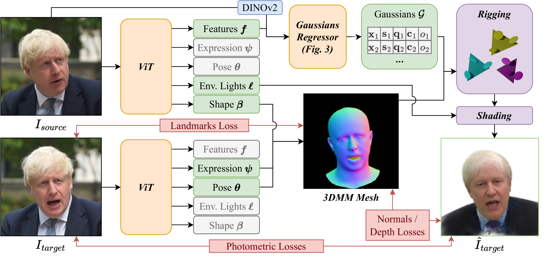
Figure 2: Overview of SHeaP. At each training step, we sample a source image $I_{\textit{source}}$ and a target image $I_{\textit{target}}$. These are both passed through the same vision transformer (ViT), which predicts 3DMM parameters shape $\bm{\beta}$, pose $\bm{\theta}$ and expression $\bm{\psi}$, plus an environment lighting latent $\bm{\ell}$ and identity features $\bm{f}$. A Gaussians Regressor takes $\bm{f}$ as input, along with DINOv2 [35] features $\mathbf{d}$. The Gaussians Regressor predicts a set of Gaussians $\mathcal{G}$, which are bound to the predicted 3DMM mesh and rendered with 2DGS to produce $\hat{I}_{\textit{target}}$. Finally, photometric losses between $\hat{I}_{\textit{target}}$ and $I_{\textit{target}}$ are backpropagated to the ViT and Gaussians Regressor parameters, as well as additional losses based on rendered depth, normals, and landmarks.

3D Gaussian Splatting (3DGS) [18] uses Gaussian primitives to represent 3D scenes, with each primitive defined by a 3D position $\bm{\mu}$ and a 3D covariance matrix $\bm{\Sigma}$. The covariance matrix $\bm{\Sigma}$ is decomposed into a rotation matrix $\mathbf{R}$ and a scaling matrix $\mathbf{S}$: $\bm{\Sigma}=\mathbf{R}\mathbf{S}\mathbf{S}^{\top}R^{\top}$. During rendering, these Gaussians are projected onto the image plane. After depth-wise sorting, a tile-based rasterizer performs $\alpha$-blending of all the $N$ primitives that overlap each pixel.

2D Gaussian Splatting (2DGS) [17] removes the third scaling dimension from 3DGS primitives, turning them into 2D surfels that resemble flat discs. 2DGS’ ray-splat intersection method to rendering allows for more precise depth maps to be computed, and it also enables closed-form modeling of each splat’s normal as the cross-product of its tangents directions. These advantages enable better geometry estimation. More specifically, each 2D Gaussian is characterized by its central point, $\bm{\mu}\in\mathbb{R}^{3}$, and two principal tangent directions, $\mathbf{t_{u}},\mathbf{t_{v}}\in\mathbb{R}^{3}$, along with their respective scales, $s_{u},s_{v}\in\mathbb{R}$. The normal direction is given by $\mathbf{t_{w}}=\mathbf{t_{u}}\times\mathbf{t_{v}}$. The rotation matrix can be expressed as $\mathbf{R}=[\mathbf{t_{u}},\mathbf{t_{v}},\mathbf{t_{w}}]$, while the scaling matrix $\mathbf{S}$ is a diagonal matrix defined as $\text{diag}(s_{u},s_{v},0)$. The 2D Gaussian lies on a plane, which can be parameterized in the $uv$-space

$$P(u,v)=\bm{\mu}+s_{u}\mathbf{t_{u}}u+s_{v}\mathbf{t_{v}}v=\mathbf{H}[u,v,1,1]^{\text{T}}\,,$$ (1)

where $\mathbf{H\in\mathbb{R}^{4\times 4}}$ is the plane parameterized with the Gaussian

$$\mathbf{H}=\begin{bmatrix}s_{u}\mathbf{t_{u}}&s_{v}\mathbf{t_{v}}&0&\bm{\mu}\\ 0&0&0&1\end{bmatrix}=\begin{bmatrix}\mathbf{R}\mathbf{S}&\bm{\mu}\\ \mathbf{0}&1\end{bmatrix}\,.$$ (2)

The opacity of a point in the $uv$-space is obtained by evaluating the Gaussian.In practice, these matrices are represented and optimized via a scaling vector $\mathbf{s}\in\mathbb{R}^{2}$ and a quaternion $\mathbf{q}\in\mathbb{R}^{4}$. In addition, each Gaussian is represented by an opacity factor $\sigma$ and a color $\mathbf{c}$. In the original implementation [18, 17], each Gaussian’s color is computed based on the viewing direction via spherical harmonics. These colors are then $\alpha$-blended to give the final pixel colors, as per 3DGS.

4 Methodology

SHeaP predicts 3DMM parameters for head geometry, and Gaussians for appearance, from a single input image. It is trained only on in-the-wild 2D videos. Training follows a self-supervised paradigm similar to DECA and other works [11, 19, 6], whereby identity information is extracted from a source frame and then re-animated with motion information from a driver frame. Photometric and landmarks losses between the ground truth and reconstructed target image provide the training signal. Our model consists of two main components (Fig. 2): the 3DMM parameter estimator and the Gaussians Regressor (Fig. 3).

4.1 3DMM Parameters Estimator

The 3DMM parameter estimator employs a transformer architecture similar to TokenFace [66]. The input face image is divided into patches, flattened and added to position embeddings to build tokens. These tokens are then passed to a vision transformer (ViT, [9]), along with five additional learnable tokens representing shape $\bm{\beta}$, expression $\bm{\psi}$, pose $\bm{\theta}$, environment lighting $\bm{\ell}$, and features $\bm{f}$ that are sent to the Gaussians Regressor (see 4.2). Layer normalization is applied at the output layer, and then a set of final MLP layers produce predictions for the various 3DMM parameter components. We initialize the ViT weights with FaRL [68].

4.2 Gaussians Regressor

The Gaussians Regressor (Fig. 3) consists of two main networks: a UV map generator that produces UV feature maps $\bm{M}$ given ViT output features $\bm{f}$ and DINOv2 features $\bm{d}$:

$$U:(\bm{f}\in\mathbb{R}^{d_{\text{features}}},\bm{d}\in\mathbb{R}^{d_{\text{DINO}}})\to\bm{M}\in\mathbb{R}^{d_{\bm{M}}\times d_{\bm{M}}\times d_{\textit{region}}}\\ ,$$

and a graph convolutional network that maps Gaussian features $\mathbf{z}$ to actual Gaussians $\mathbf{g}$:

$$\bm{F}:\mathbf{z}\in\mathbb{R}^{N_{G}\times d_{\mathbf{z}}}\to\mathbf{g}\in\mathbb{R}^{N_{G}\times d_{\mathbf{g}}}\\ .$$

We process the source image through our ViT and take its output $\bm{f}$, and reshape this to a feature map which serves as input to a Lightweight GAN [28] architecture. This network cross-attends to DINOv2 features [35], also extracted from the source image, and produces a $d_{\bm{M}}\times d_{\bm{M}}\times d_{\textit{region}}$ tensor of UV features: $\bm{M}$.

The goal now is to generate a set of $N_{G}$ Gaussians $\mathcal{G}$, which we will later bind to the 3DMM mesh for rendering. To initialize our set of Gaussians, we assign $N_{G}^{\textit{init}}$ Gaussians to each face of the mesh. We refer to the $i$-th Gaussian’s parent face index as $p_{i}$. At initialization, each Gaussian also gets a unique learnable embedding vector $\bm{e}_{i}$. This is concatenated with ‘region’ features $\bm{r}_{i}$, which are computed by sampling the generated UV feature map $\bm{M}$:

$$\bm{r}_{i}=\textit{GridSample}(\bm{M},p_{i},\bm{V})\\ ,$$ (3)

where the GridSample operator here samples the features $\bm{M}$ according to the location of Gaussian $i$’s parent face $p_{i}$ in the 3DMM’s fixed UV map $\bm{V}$.

We concatenate the embedding $\bm{e}_{i}$ with these region features $\bm{r}_{i}$ to produce Gaussian features $\mathbf{z}_{i}$. We want nearby Gaussians to be able to communicate and organize among themselves. To this end, we employ a graph convolutional neural network. This network takes on a ResNet-style architecture [16], with graph-convolution [33] operations replacing convolution operations. The adjacency matrix between Gaussians $i$ and $j$ with parent faces $p_{i}$ and $p_{j}$ is defined as:

$$A_{ij}=\begin{cases}1,&\text{if }p_{j}\in\textit{neighbors}(p_{i},\mathcal{D})\\ 0,&\text{otherwise}\end{cases}\\ ,$$ (4)

where the $\textit{neighbors}(f,\mathcal{D})$ function finds all neighbors of mesh face $f$ up to degree $\mathcal{D}$ (we set $\mathcal{D}=2$).

The graph convolutional neural network takes as input the adjacency matrix, along with the embeddings and region features, and produces the Gaussians to be rendered. Each Gaussian is defined by 13 values: an offset from the parent face ($\mathbf{x}_{i}\in\mathbb{R}^{3}$); a scale ($\mathbf{s}_{i}\in\mathbb{R}^{3}$); a rotation quaternion ($\mathbf{q}_{i}\in\mathbb{R}^{4}$); an albedo color ($\mathbf{c}_{i}\in\mathbb{R}^{3}$); and an opacity scalar ($\sigma_{i}$). These Gaussians are then rigged to the 3DMM as described in Section 4.4.

Figure 3: Architecture of the Gaussians generator. In the illustrated case, the first two Gaussians have the same parent face: $p_{1}=p_{2}$ and thus their learned embeddings $\bm{e}_{1},\bm{e}_{2}$ are concatenated with the same region features, $\mathbf{r}_{1}$.

4.3 Gaussians Densification and Pruning

Our novel Gaussians Regressor architecture allows the set of Gaussians $\mathcal{G}$ to undergo a densification and pruning process, like the original 3DGS paper [18]. However, rather than densifying and pruning actual Gaussians, we densify and prune the latent features that produce these Gaussians.

As introduced in Section 4.2, each Gaussian is produced by a parent face $p_{i}$ and an embedding $\bm{e}_{i}$. Together, we refer to these as Gaussian ‘prototypes’. For each prototype, we track the opacity values and positional gradients of the Gaussians it produces. Every $t_{\textit{densify}}$ iterations, we take the $n_{\textit{prune}}$ prototypes with the lowest average predicted opacity values and delete them from $\mathcal{G}$. We then make a copy of the prototypes that received the largest average positional gradients during the last $t_{\textit{history}}$ iterations. We then add a small amount of noise to the embeddings of the copied prototypes $\bm{e}_{i}$, and add them to $\mathcal{G}$. We typically set $n_{\textit{prune}}=n_{\textit{densify}}$, which keeps the total number of Gaussians constant. We also enforce that each face on the mesh has at least one Gaussian attached to it, and at most six.

4.4 Binding Gaussians to 3DMM and Shading

Binding.

We build upon the GaussianAvatars binding formulation [41] by adapting it to 2DGS [17]. In this model[41], Gaussians are anchored to an underlying 3DMM mesh, enabling the avatar to be animated using 3DMM parameters. Each Gaussian is linked to a specific parent triangle in a canonical (local) space. During rendering in a deformed space, each Gaussian undergoes transformations based on its parent’s current state, including the relative rotation matrix $\mathbf{R_{p}}$, the isotropic scale determined by the relative area of the triangle $s_{p}$, and the centroid of the triangle $\bm{\mu_{p}}$ in world space. In contrast to GaussianAvatars [41], our method necessitates a precise correspondence between each Gaussian and its parent triangle. This precision is essential for accurately aligning the 3DMM geometry with the appearance data derived from the Gaussians. To achieve this, we refined the parent triangle scaling to an anisotropic scale vector $\mathbf{s_{p}}=[s_{p,u},s_{p,v},s_{p,n}]$. Here, $s_{p,u}$ and $s_{p,v}$ represent the length of the triangle in the UV directions defined by the matrix $\mathbf{R_{p}}$. The scale in the normal direction of the triangle $s_{p,n}$ is defined as the minimum between $s_{p,u}$ and $s_{p,v}$. The scaling matrix of the parent triangle is defined as $\mathbf{S_{p}}=\text{diag}(s_{p,u},s_{p,v},0)$. The transformations are given by the equations

$$\mathbf{R}=\mathbf{R_{p}}\mathbf{R_{c}}\quad\bm{\mu}=\mathbf{R_{p}}\mathbf{s_{p}}\bm{\mu}_{c}+\bm{\mu_{p}}\quad\mathbf{S}=\mathbf{S_{p}}\mathbf{S_{c}}$$ (5)

where $\mathbf{R_{c}}$ represents canonical rotations, $\bm{\mu_{c}}$ the canonical position, and $\mathbf{S_{c}}$ the canonical scaling of the parent’s triangle. Note that while the scaling matrix $\mathbf{S_{p}}$, with a null scale in the normal direction, affects the final scale $\mathbf{S}$, the scaling vector $\mathbf{s_{p}}$, which affects the Gaussian’s position $\bm{\mu}$, has a non-null normal scale. This allows the Gaussian to move outside the mesh, capturing regions and details not modeled by the underlying 3DMM.

Illumination Model.

For Gaussian $i$, the Gaussians Regressor outputs an RGB albedo color $\mathbf{a}_{i}\in\mathbb{R}^{3}$. To compute the final color of each splat, we combine this with a Lambertian shading model based on Spherical Harmonics (SH) [50]. The ViT predicts a vector of lighting principal component weights from the source image: $\bm{\ell}_{\textit{source}}$. These weights are then transformed into spherical harmonics coefficients $\bm{w}_{SH}$ via the Basel Illumination Prior [10] PCA space $\bm{w}^{SH}=\bm{P}\bm{\ell}_{\textit{source}}$, where $\bm{P}$ is a $D\times 27$ matrix of eigenvectors. Splitting these weights by color channel $j$, we compute the final color

$$c_{ij}=a_{ij}\sum_{k=1}^{9}w_{jk}^{SH}SH_{k}(N_{i})\,,$$ (6)

where $\mathcal{N}_{i}$ is the normal of the $i$’th 2D Gaussian (computed as the cross product of its tangent vectors), and $SH_{k}:\mathbb{R}^{3}\to\mathbb{R}$ defines the SH basis and coefficients.

4.5 2D Self-Supervised Loss Functions

After predicting our 3DMM, Gaussians, and rendered image, we can compute a number of self-supervised loss functions by comparing aspects of the rendered images to their ground truth. Unless otherwise stipulated, these losses pertain to the target image and not the source image.

4.5.1 Landmarks Loss

We calculate an L1 loss between the projected landmarks of our predicted mesh and 2D landmarks from third party models ([2], [29]). We do not perform occlusion or head pose filtering on these landmarks; we just employ a very small loss weight on the landmarks loss, which prevents inaccuracies from having too large of an effect on the model.

4.5.2 Photometric Losses

We compute four photometric losses between $I_{\text{target}}$ and $\hat{I}_{\text{target}}$, and denote these together as $\mathcal{L}_{\text{photo}}$:

$$\mathcal{L}_{\textit{photo}}=w_{\text{L1}}\mathcal{L}_{\textit{L1}}+w_{\text{perc}}\mathcal{L}_{\textit{perc}}+w_{\text{ID}}\mathcal{L}_{\textit{ID}}+w_{\text{emo}}\mathcal{L}_{\textit{exp}}\,,$$ (7)

Before computing any of these losses, the background is removed from the target image (using [5]) and replaced with the same random color used as the background when rendering the Gaussians.

L1 Photometric Loss is computed as:

$$\mathcal{L}_{\textit{L1}}=\lvert(I_{\text{target}}-\hat{I}_{\text{target}})(0.7M_{\text{face}}+0.3)\rvert\,,$$ (8)

where $M_{\text{face}}$ is a per-pixel mask (predicted with [23]) which equals $1$ in the face region and $0$ elsewhere.

Perceptual Loss. Here we employ the same facial perceptual loss as [6]. The loss is computed as:

$$\mathcal{L}_{\textit{perc}}=\lvert P(I_{\text{target}})-P(\hat{I}_{\text{target}})\rvert\,,$$ (9)

where $P$ computes features at various layers from a VGGFace network [4].

Identity Divergence Loss is computed as the cosine similarity of Arcface features computed on the facial region:

$$\mathcal{L}_{\textit{ID}}=1-\frac{f_{\text{ID}}(I_{\text{target}})f_{\text{ID}}(\hat{I}_{\text{target}})}{\lVert f_{\text{ID}}(I_{\text{target}})\cdot f_{\text{ID}}(\hat{I}_{\text{target}})\rVert_{2}}\,.$$ (10)

Facial Expression Loss is computed as per the identity divergence loss, with features extracted instead from a facial expression recognition network [49] $f_{\text{exp}}$:

$$\mathcal{L}_{\textit{exp}}=1-\frac{f_{\text{exp}}(I_{\text{target}})f_{\text{exp}}(\hat{I}_{\text{target}})}{\lVert f_{\text{exp}}(I_{\text{target}})\cdot f_{\text{exp}}(\hat{I}_{\text{target}})\rVert_{2}}\,.$$ (11)

4.5.3 Gaussians vs. 3DMM Geometric Coupling Loss

We wish to encourage a tight coupling between the 3DMM mesh’s geometry and that implied by the Gaussians. To achieve this, we introduce regularization on the rendered normals and depth maps of the 3DMM and Gaussians.

The normal of a given 2D Gaussian is computed as the cross-product of its two tangent vectors. 2DGS rendering thus can compute a normal image by alpha-blending the normals of all primitive along a pixel’s ray. We penalize the L1 distance between the rendered 3DMM mesh normals $N_{\text{3DMM}}$, and the rendered Gaussian normals $N_{\text{2DGS}}$ (masking out non-facial regions):

$$\mathcal{L}_{\textit{normals}}=\lvert(N_{\text{2DGS}}-N_{\text{3DMM}})\cdot M_{\text{face}}\rvert\,,.$$ (12)

To further enforce this geometric similarity between the Gaussians and the 3DMM mesh, we also render depth and compute another L1 loss:

$$\mathcal{L}_{\textit{depth}}=\lvert(D_{\text{2DGS}}-D_{\text{3DMM}})\cdot M_{\text{face}}\rvert\,,$$ (13)

where $D_{\text{2DGS}}$ is the depth rendered from the 2D Gaussians representation.

4.5.4 Regularizers

Gaussian Regularizers. We penalise the L2 norm of the offset $\bm{x}_{i}$ and scale $\bm{s}_{i}$ of the predicted Gaussians. As per [22], to encourage Gaussians to be either fully transparent or opaque, we also regularize opacity. The total Gaussians regularization loss is:

$$\mathcal{L}_{\textit{reg}}^{\textit{Gau}}=\sum_{i=0}^{N_{G}}\Big{(}w_{\bm{x}}\lVert\bm{x}_{i}\rVert_{2}+w_{\bm{s}}\lVert\bm{s}_{i}\rVert_{2}+w_{o}\textit{Beta}(o_{i})\Big{)}\,,$$ (14)

where Beta is the negative log-likelihood of a Beta(0.5, 0.5) distribution.

3DMM Regularizers. We regularize the L2 norm of the predicted 3DMM shape and expression codes:

$$\mathcal{L}_{\textit{reg}}^{\textit{3DMM}}=w_{\bm{\psi}}\cdot\lVert\bm{\psi}\rVert_{2}+w_{\bm{\beta}}\cdot\lVert\bm{\beta}\rVert_{2}\,.$$ (15)

5 Experimental Setup

Training Datasets.

We train with VFHQ [62] and Nersemble [21]. Although Nersemble is a multi-view dataset, we do not make use of its camera extrinsics data, essentially treating it as 2D data. At each training step, we sample a random image to be the source image, and then another random image from the same video to be the target image. We sample from VFHQ [62] 75% of the time and Nersemble [21] 25% of the time.

Evaluation Methods.

We use two datasets for geometric evaluation; both of which require a 3D mesh to be predicted given a single image of a person’s face. The predicted 3D mesh is then rigidly aligned to a ground truth scan, and the reported metric is the median and mean distance in millimeters from each point in that scan to a large number of random points sampled from the surface of the mesh. If a scaling factor is fit during this rigid alignment process, then a ‘non-metrical‘ evaluation is being performed; otherwise, the evaluation assumes the predicted mesh is already to scale and thus it is a ‘metrical’ evaluation. Here we focus on non-metrical evaluation.

We evaluate neutral geometry on the NoW dataset [47]. To evaluate non-neutral expressions, we construct a new evaluation metric based on metric-accurate point clouds extracted from Nersemble [21]. In Nersemble, dense point clouds estimated with COLMAP [48] are provided for several multi-view frames for 10 subjects. We filter these point clouds to only contain points in the face region, and exclude frames with low confidence, resulting in 60 high-quality point clouds with 960 images captured from different views. For each of these timesteps, we retrieve the multi-view images for which a face is visible, and predict the head mesh geometry with all comparison methods. Like in NoW [47], we evaluate each method by rigidly aligning the predicted meshes with the ground truth point clouds. We report the median and mean L2 distance in mm from each point in the cloud to its nearest point on the mesh surface.

Finally, we measure the emotional content of the meshes predicted by SHeaP, by evaluating on AffectNet [31]. We follow EMOCA’s [7] approach and first predict 3DMM parameters for all images in the AffectNet dataset, and then fit a 4-layer MLP to predict valence, arousal, and emotion category, based only on these parameters. Our quantitative results are reported in Section 6.2. Further implementation details are provided in the supplementary material.

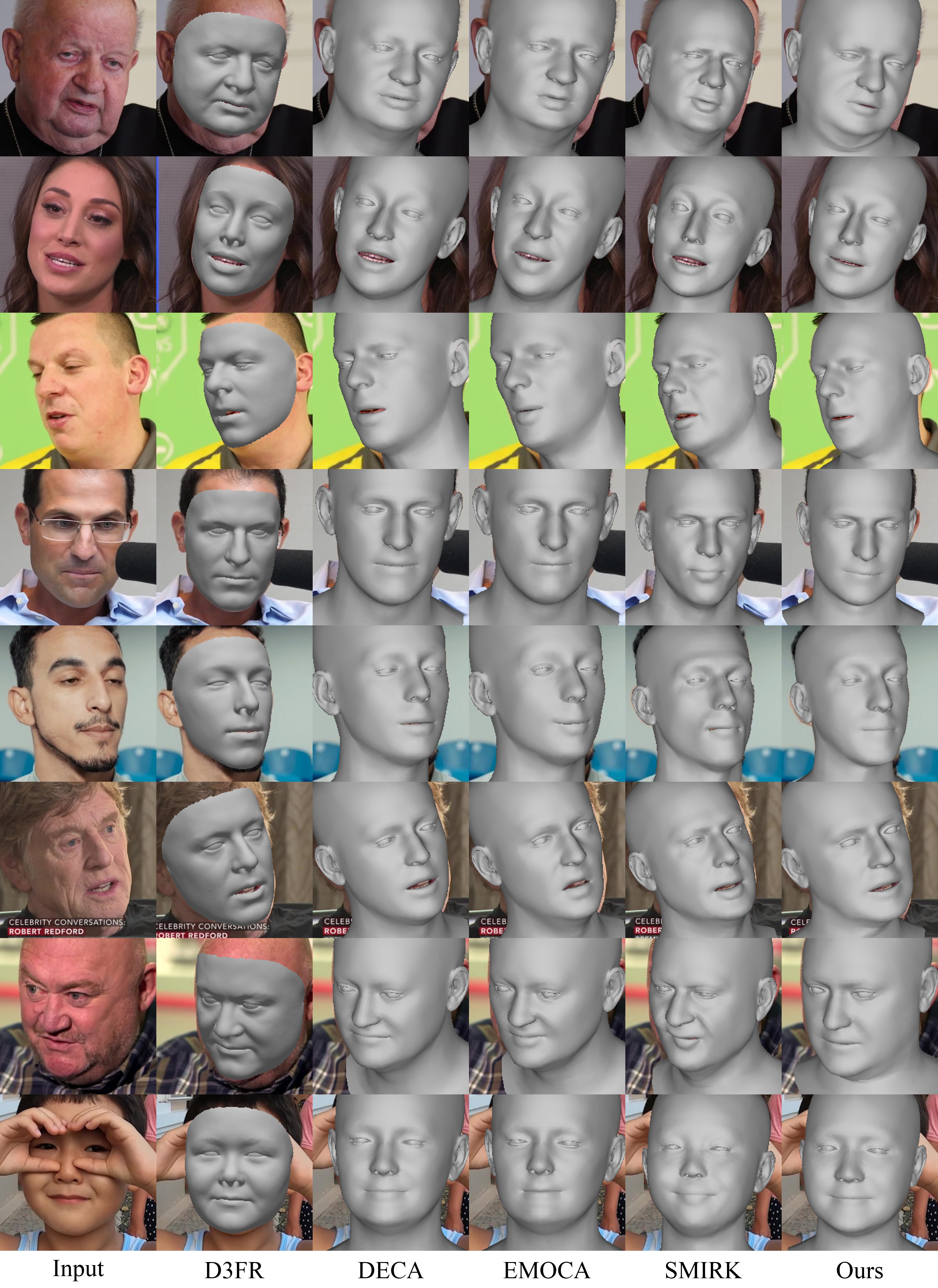
Figure 4: Comparison to other one-shot reconstruction methods, from left to right: Deep3DFaceRecon [8], DECA [11], EMOCA [7], SMIRK [44], Ours.

Implementation Details.

Our method is implemented in PyTorch [38] and uses Pytorch3D [43] and gsplat [65]. We use the Adam optimizer [20], with a learning rate of 1e-3 for everything except the ViT, which uses 1e-5. Images are compared and rendered at 512x512 resolution, but are resized to 224x224 for the ViT and 448x448 for DINOv2 feature extraction. Preprocessing steps involve cropping to the facial region, and predicting facial landmarks [29, 2], face segmentation maps [23], and background segmentation maps [5]. For rendering of both Gaussians and meshes, we fix the FOV degrees to 14.3, which is the median FOV degrees of Nersemble data downsampled by a factor of 4 and center-cropped to 512x512. Additional details and results are provided in the supplementary materials.

6 Results

Method	Only 2D	Distance (mm)
	Supervision	Median	Mean
Deep3DFaceRecon [8]	✓	1.11	1.4
DECA [11]	✓	1.09	1.38
CCFace [64]	✓	1.08	1.35
FOCUS [26]	✓	1.04	1.30
DenseLandmark [59]	✓	1.02	1.28
AlbedoGAN [42]	✓	0.98	1.21
Ours	✓	0.95	1.18
1-4 MICA [69]	✗	0.90	1.11
FlowFace [55]	✗	0.87	1.07
TokenFace [66]	✗	0.78	0.95

Table 1: Non-metrical evaluation on the NoW Test Set. Our method achieves state-of-the-art error rates among methods that rely only on 2D supervision. Methods below the dashed line use 3D supervision.

6.1 Qualitative Evaluation

SHeaP reconstructs 3D head geometry, pose and expression given a single face image. Fig. 4 qualitatively compares SHeaP with other state-of-the-art methods, namely Deep 3D Face Reconstruction (Pytorch implementation, [8]), DECA [11], EMOCA [7] and SMIRK [44]. SHeaP produces more plausible geometry that better aligns with the input image. Our method is also the only method capable of disentangling neck from torso pose; all other methods keep the neck joint fixed, rotating the entire torso to align the facial region. This enhances the reconstruction realism and the the overall alignment of the predicted mesh. SHeaP also predicts realistic and accurate facial expressions, which are focused on accurate geometry reconstruction rather than producing exaggerated expressions. This is key to SHeaP’s quantitative performance, described in the next section.

6.2 Quantitative Evaluation

We compare SHeaP with other publicly-available models, namely DECA [11], EMOCA [7], SMIRK [44], Deep3DFaceRecon [8] and FOCUS [26].

NoW Evaluation.

Our results on NoW test set are presented in Table 1. SHeaP outperforms all other methods that rely on only 2D supervision to train their head geometry predictor. Other methods, like TokenFace, show impressive performance, but these rely on using 3D scan data for direct supervision. SHeaP’s performance shows promise in the direction of using more scalable 2D data for learning to predict geometry.

Nersemble Evaluation.

The NoW dataset only assesses a method’s ability to reconstruct a person’s head geometry under a neutral expression. To evaluate each method’s ability to reconstruct expressive head geometry, we evaluated them through our new Nersemble benchmark introduced in Section 5. As shown in Table 2, SHeaP outperforms all competing methods by a fairly substantial margin, highlighting its ability to predict accurate geometry even under varying poses and expressions.

Method	Distance (mm)
	Mean	Median	Std
DECA [11]	2.46	2.46	0.46
EMOCA [7]	2.58	2.54	0.46
SMIRK [44]	2.30	2.24	0.42
Ours	2.18	2.12	0.40

Table 2: Distance metrics on our Nersemble-based [21] reconstruction benchmark. Note that SMIRK [44] uses MICA [69] for its shape code.

AffectNet.

Finally, we evaluate the capacity of our model’s estimated 3DMM parameters to predict emotion. Following EMOCA [7], and as described in Section 5, we use SHeaP and competing methods to predict 3DMM parameters for all of AffectNet. We then fit a 4-layer MLP to the training portion of these parameters, and evaluate on the test set. The results (Table 3) show that the 3DMM parameters predicted by SHeaP are rich in emotional content, outperforming both SMIRK [44] and EMOCA [7] in emotion prediction on AffectNet.

Model	Valence		Arousal		Emo
	CCC↑	RMSE↓	CCC↑	RMSE↓	Acc.
SMIRK [44]	0.56	0.29	0.68	0.31	0.65
EMOCA [7]	0.58	0.28	0.70	0.31	0.68
Ours	0.62	0.27	0.74	0.30	0.70

Table 3: Emotion recognition performance on AffectNet [32], we report the concordance correlation coefficient (CCC) and root mean squared error (RMSE) on predicting Valence and Arousal, plus accuracy in 8-way emotion classification.

6.3 Ablation Study

We perform an ablation over the most important hyperparameters of our method (Table 4). With only photometric loss and basic regularization, our method still outperforms DECA on the NoW validation set (median of 1.18mm [11]), highlighting the effectiveness of Gaussians in comparison to differentiable mesh rendering for this type of task. Error rates can be greatly improved, however, by adding perceptual losses, most notably the identity perceptual loss. The impact of $\mathcal{L}_{\textit{normals}}+\mathcal{L}_{\textit{depth}}$ illustrates the importance of encouraging a tight coupling of the Gaussians geometry with that of the 3DMM. Finally the visual improvements thanks to densification and pruning, enabled by our novel architecture, add a final additional boost to performance.

$\mathcal{L}_{\textit{perc}}$	$\mathcal{L}_{\textit{ID}}$	Densification	$\mathcal{L}_{\textit{normals}}$	Distance (mm)
		and Pruning	$+\mathcal{L}_{\textit{depth}}$	Median	Mean
✗	✗	✗	✗	1.09	1.38
✓	✗	✗	✗	1.06	1.31
✓	✗	✓	✓	1.03	1.25
✓	✓	✗	✗	0.99	1.22
✓	✓	✓	✗	0.98	1.21
✓	✓	✗	✓	0.96	1.20
✓	✓	✓	✓	0.93	1.16

Table 4: Ablation study results on the NoW Validation Set. The table shows active components with checkmarks and corresponding distances.

7 Conclusion

In this paper, we introduced SHeaP, a novel method for 3D head reconstruction and animation from monocular images using self-supervised learning and advanced neural rendering. By employing 3DMM-rigged Gaussian Splatting, SHeaP achieves enhanced accuracy in photometric loss computation, leading to superior performance across multiple benchmarks.

Despite this, our method faces certain limitations. While our Gaussian-based representation offers stronger photometric supervision compared to textured meshes, it still faces challenges in fully leveraging the potential of the Gaussian Splatting representation, potentially due to alignment issues in one-shot geometry prediction. Additionally, the lack of 3D supervision results in scale-free meshes, and the fixed-FOV assumption forces our model to use the predicted head shape to model head distortions owing to FOV differences. Future work could explore incorporating offline refinement of the predicted 3DMM meshes before rendering the rigged Gaussians. This may address shortcomings of feedforward prediction and lead to sharper renderings. Training with multiview data or direct 3D supervision is another promising direction. Finally, our method might benefit from an accurate image-based FOV predictor, like in [39].

Overall, SHeaP represents a significant step forward in the field of learning self-supervised 3D head reconstruction and animation from 2D data, providing a foundation for future advancements and applications.

References

- Blanz and Vetter [2023] Volker Blanz and Thomas Vetter. A morphable model for the synthesis of 3d faces. In Seminal Graphics Papers: Pushing the Boundaries, Volume 2, pages 157–164. 2023.
- Bulat and Tzimiropoulos [2017] Adrian Bulat and Georgios Tzimiropoulos. How far are we from solving the 2d & 3d face alignment problem? (and a dataset of 230,000 3d facial landmarks). In International Conference on Computer Vision, 2017.
- Cao et al. [2018a] Chen Cao, Menglei Chai, Oliver Woodford, and Linjie Luo. Stabilized real-time face tracking via a learned dynamic rigidity prior. ACM Transactions on Graphics (TOG), 37(6):1–11, 2018a.
- Cao et al. [2018b] Qiong Cao, Li Shen, Weidi Xie, Omkar M Parkhi, and Andrew Zisserman. Vggface2: A dataset for recognising faces across pose and age. In 2018 13th IEEE international conference on automatic face & gesture recognition (FG 2018), pages 67–74. IEEE, 2018b.
- Chicherin and Efremyan [2023] Sergej Chicherin and Karen Efremyan. Adversarially-guided portrait matting. arXiv preprint arXiv:2305.02981, 2023.
- Chu and Harada [2024] Xuangeng Chu and Tatsuya Harada. Generalizable and animatable gaussian head avatar. arXiv preprint arXiv:2410.07971, 2024.
- Danecek et al. [2022] Radek Danecek, Michael J. Black, and Timo Bolkart. EMOCA: Emotion driven monocular face capture and animation. In Conference on Computer Vision and Pattern Recognition (CVPR), pages 20311–20322, 2022.
- Deng et al. [2019] Yu Deng, Jiaolong Yang, Sicheng Xu, Dong Chen, Yunde Jia, and Xin Tong. Accurate 3d face reconstruction with weakly-supervised learning: From single image to image set. In IEEE Computer Vision and Pattern Recognition Workshops, 2019.
- Dosovitskiy et al. [2020] Alexey Dosovitskiy, Lucas Beyer, Alexander Kolesnikov, Dirk Weissenborn, Xiaohua Zhai, Thomas Unterthiner, Mostafa Dehghani, Matthias Minderer, Georg Heigold, Sylvain Gelly, et al. An image is worth 16x16 words: Transformers for image recognition at scale. arXiv preprint arXiv:2010.11929, 2020.
- Egger et al. [2018] Bernhard Egger, Sandro Schönborn, Andreas Schneider, Adam Kortylewski, Andreas Morel-Forster, Clemens Blumer, and Thomas Vetter. Occlusion-aware 3d morphable models and an illumination prior for face image analysis. International Journal of Computer Vision, 126:1269–1287, 2018.
- Feng et al. [2021] Yao Feng, Haiwen Feng, Michael J. Black, and Timo Bolkart. Learning an animatable detailed 3D face model from in-the-wild images. ACM Transactions on Graphics (ToG), Proc. SIGGRAPH, 40(4):88:1–88:13, 2021.
- Gafni et al. [2021] Guy Gafni, Justus Thies, Michael Zollhöfer, and Matthias Nießner. Dynamic neural radiance fields for monocular 4d facial avatar reconstruction. In Proceedings of the IEEE/CVF Conference on Computer Vision and Pattern Recognition (CVPR), pages 8649–8658, 2021.
- Giebenhain et al. [2023] Simon Giebenhain, Tobias Kirschstein, Markos Georgopoulos, Martin Rünz, Lourdes Agapito, and Matthias Nießner. Learning neural parametric head models. In Proceedings of the IEEE/CVF Conference on Computer Vision and Pattern Recognition, pages 21003–21012, 2023.
- Giebenhain et al. [2024] Simon Giebenhain, Tobias Kirschstein, Martin Rünz, Lourdes Agapito, and Matthias Nießner. Npga: Neural parametric gaussian avatars. In SIGGRAPH Asia 2024 Conference Papers (SA Conference Papers ’24), December 3-6, Tokyo, Japan, 2024.
- He et al. [2016a] Kaiming He, Xiangyu Zhang, Shaoqing Ren, and Jian Sun. Deep residual learning for image recognition. In Proceedings of the IEEE conference on computer vision and pattern recognition, pages 770–778, 2016a.
- He et al. [2016b] Kaiming He, Xiangyu Zhang, Shaoqing Ren, and Jian Sun. Deep residual learning for image recognition. In Proceedings of the IEEE conference on computer vision and pattern recognition, pages 770–778, 2016b.
- Huang et al. [2024] Binbin Huang, Zehao Yu, Anpei Chen, Andreas Geiger, and Shenghua Gao. 2d gaussian splatting for geometrically accurate radiance fields. In SIGGRAPH 2024 Conference Papers. Association for Computing Machinery, 2024.
- Kerbl et al. [2023] Bernhard Kerbl, Georgios Kopanas, Thomas Leimkühler, and George Drettakis. 3d gaussian splatting for real-time radiance field rendering. ACM Transactions on Graphics, 42(4), 2023.
- Khakhulin et al. [2022] Taras Khakhulin, Vanessa Sklyarova, Victor Lempitsky, and Egor Zakharov. Realistic one-shot mesh-based head avatars. In European Conference of Computer vision (ECCV), 2022.
- Kingma and Ba [2014] Diederik P Kingma and Jimmy Ba. Adam: A method for stochastic optimization. arXiv preprint arXiv:1412.6980, 2014.
- Kirschstein et al. [2023] Tobias Kirschstein, Shenhan Qian, Simon Giebenhain, Tim Walter, and Matthias Nießner. Nersemble: Multi-view radiance field reconstruction of human heads. ACM Trans. Graph., 42(4), 2023.
- Kirschstein et al. [2024] Tobias Kirschstein, Simon Giebenhain, Jiapeng Tang, Markos Georgopoulos, and Matthias Nießner. Gghead: Fast and generalizable 3d gaussian heads. In SIGGRAPH Asia 2024 Conference Papers, pages 1–11, 2024.
- Kvanchiani et al. [2023] Karina Kvanchiani, Elizaveta Petrova, Karen Efremyan, Alexander Sautin, and Alexander Kapitanov. Easyportrait–face parsing and portrait segmentation dataset. arXiv preprint arXiv:2304.13509, 2023.
- Laine et al. [2020] Samuli Laine, Janne Hellsten, Tero Karras, Yeongho Seol, Jaakko Lehtinen, and Timo Aila. Modular primitives for high-performance differentiable rendering. ACM Transactions on Graphics (ToG), 39(6):1–14, 2020.
- Lei et al. [2023] Biwen Lei, Jianqiang Ren, Mengyang Feng, Miaomiao Cui, and Xuansong Xie. A hierarchical representation network for accurate and detailed face reconstruction from in-the-wild images. In Proceedings of the IEEE/CVF Conference on Computer Vision and Pattern Recognition, pages 394–403, 2023.
- Li et al. [2023] Chunlu Li, Andreas Morel-Forster, Thomas Vetter, Bernhard Egger, and Adam Kortylewski. Robust model-based face reconstruction through weakly-supervised outlier segmentation. In Proceedings of the IEEE/CVF Conference on Computer Vision and Pattern Recognition, pages 372–381, 2023.
- Li et al. [2017] Tianye Li, Timo Bolkart, Michael. J. Black, Hao Li, and Javier Romero. Learning a model of facial shape and expression from 4D scans. ACM Transactions on Graphics, (Proc. SIGGRAPH Asia), 36(6):194:1–194:17, 2017.
- Liu et al. [2021] Bingchen Liu, Yizhe Zhu, Kunpeng Song, and Ahmed Elgammal. Towards faster and stabilized gan training for high-fidelity few-shot image synthesis. In iclr, 2021.
- Lugaresi et al. [2019] Camillo Lugaresi, Jiuqiang Tang, Hadon Nash, Chris McClanahan, Esha Uboweja, Michael Hays, Fan Zhang, Chuo-Ling Chang, Ming Yong, Juhyun Lee, Wan-Teh Chang, Wei Hua, Manfred Georg, and Matthias Grundmann. Mediapipe: A framework for perceiving and processing reality. In Third Workshop on Computer Vision for AR/VR at IEEE Computer Vision and Pattern Recognition (CVPR) 2019, 2019.
- Mildenhall et al. [2020] Ben Mildenhall, Pratul P. Srinivasan, Matthew Tancik, Jonathan T. Barron, Ravi Ramamoorthi, and Ren Ng. Nerf: Representing scenes as neural radiance fields for view synthesis. In ECCV, 2020.
- Mollahosseini et al. [2017a] Ali Mollahosseini, Behzad Hasani, and Mohammad H Mahoor. Affectnet: A database for facial expression, valence, and arousal computing in the wild. IEEE Transactions on Affective Computing, 10(1):18–31, 2017a.
- Mollahosseini et al. [2017b] Ali Mollahosseini, Behzad Hasani, and Mohammad H Mahoor. Affectnet: A database for facial expression, valence, and arousal computing in the wild. IEEE Transactions on Affective Computing, 10(1):18–31, 2017b.
- Morris et al. [2019] Christopher Morris, Martin Ritzert, Matthias Fey, William L Hamilton, Jan Eric Lenssen, Gaurav Rattan, and Martin Grohe. Weisfeiler and leman go neural: Higher-order graph neural networks. In Proceedings of the AAAI conference on artificial intelligence, pages 4602–4609, 2019.
- Müller et al. [2022] Thomas Müller, Alex Evans, Christoph Schied, and Alexander Keller. Instant neural graphics primitives with a multiresolution hash encoding. ACM Trans. Graph., 41(4):102:1–102:15, 2022.
- Oquab et al. [2023] Maxime Oquab, Timothée Darcet, Théo Moutakanni, Huy Vo, Marc Szafraniec, Vasil Khalidov, Pierre Fernandez, Daniel Haziza, Francisco Massa, Alaaeldin El-Nouby, et al. Dinov2: Learning robust visual features without supervision. arXiv preprint arXiv:2304.07193, 2023.
- Park et al. [2021a] Keunhong Park, Utkarsh Sinha, Jonathan T. Barron, Sofien Bouaziz, Dan B Goldman, Steven M. Seitz, and Ricardo Martin-Brualla. Nerfies: Deformable neural radiance fields. ICCV, 2021a.
- Park et al. [2021b] Keunhong Park, Utkarsh Sinha, Peter Hedman, Jonathan T. Barron, Sofien Bouaziz, Dan B Goldman, Ricardo Martin-Brualla, and Steven M. Seitz. Hypernerf: A higher-dimensional representation for topologically varying neural radiance fields. ACM Trans. Graph., 40(6), 2021b.
- Paszke et al. [2019] Adam Paszke, Sam Gross, Francisco Massa, Adam Lerer, James Bradbury, Gregory Chanan, Trevor Killeen, Zeming Lin, Natalia Gimelshein, Luca Antiga, et al. Pytorch: An imperative style, high-performance deep learning library. Advances in neural information processing systems, 32, 2019.
- Patel and Black [2024] Priyanka Patel and Michael J Black. Camerahmr: Aligning people with perspective. arXiv preprint arXiv:2411.08128, 2024.
- Paysan et al. [2009] Pascal Paysan, Reinhard Knothe, Brian Amberg, Sami Romdhani, and Thomas Vetter. A 3d face model for pose and illumination invariant face recognition. In 2009 sixth IEEE international conference on advanced video and signal based surveillance, pages 296–301. Ieee, 2009.
- Qian et al. [2024] Shenhan Qian, Tobias Kirschstein, Liam Schoneveld, Davide Davoli, Simon Giebenhain, and Matthias Nießner. Gaussianavatars: Photorealistic head avatars with rigged 3d gaussians. In Proceedings of the IEEE/CVF Conference on Computer Vision and Pattern Recognition, pages 20299–20309, 2024.
- Rai et al. [2024] Aashish Rai, Hiresh Gupta, Ayush Pandey, Francisco Vicente Carrasco, Shingo Jason Takagi, Amaury Aubel, Daeil Kim, Aayush Prakash, and Fernando De la Torre. Towards realistic generative 3d face models. In Proceedings of the IEEE/CVF Winter Conference on Applications of Computer Vision, pages 3738–3748, 2024.
- Ravi et al. [2020] Nikhila Ravi, Jeremy Reizenstein, David Novotny, Taylor Gordon, Wan-Yen Lo, Justin Johnson, and Georgia Gkioxari. Accelerating 3d deep learning with pytorch3d. arXiv:2007.08501, 2020.
- Retsinas et al. [2024] George Retsinas, Panagiotis P. Filntisis, Radek Danecek, Victoria F. Abrevaya, Anastasios Roussos, Timo Bolkart, and Petros Maragos. 3d facial expressions through analysis-by-neural-synthesis. In Conference on Computer Vision and Pattern Recognition (CVPR), 2024.
- Ruan et al. [2021] Zeyu Ruan, Changqing Zou, Longhai Wu, Gangshan Wu, and Limin Wang. Sadrnet: Self-aligned dual face regression networks for robust 3d dense face alignment and reconstruction. IEEE Transactions on Image Processing, 30:5793–5806, 2021.
- Sandler et al. [2018] Mark Sandler, Andrew Howard, Menglong Zhu, Andrey Zhmoginov, and Liang-Chieh Chen. Mobilenetv2: Inverted residuals and linear bottlenecks. In Proceedings of the IEEE conference on computer vision and pattern recognition, pages 4510–4520, 2018.
- Sanyal et al. [2019] Soubhik Sanyal, Timo Bolkart, Haiwen Feng, and Michael Black. Learning to regress 3D face shape and expression from an image without 3D supervision. In Proceedings IEEE Conf. on Computer Vision and Pattern Recognition (CVPR), pages 7763–7772, 2019.
- Schönberger et al. [2016] Johannes Lutz Schönberger, Enliang Zheng, Marc Pollefeys, and Jan-Michael Frahm. Pixelwise view selection for unstructured multi-view stereo. In European Conference on Computer Vision (ECCV), 2016.
- Schoneveld and Othmani [2021] Liam Schoneveld and Alice Othmani. Towards a general deep feature extractor for facial expression recognition. In 2021 IEEE International Conference on Image Processing (ICIP), pages 2339–2342. IEEE, 2021.
- Seeley [1966] Robert T Seeley. Spherical harmonics. The American Mathematical Monthly, 73(4P2):115–121, 1966.
- Shao et al. [2024] Zhijing Shao, Zhaolong Wang, Zhuang Li, Duotun Wang, Xiangru Lin, Yu Zhang, Mingming Fan, and Zeyu Wang. Splattingavatar: Realistic real-time human avatars with mesh-embedded gaussian splatting. In Proceedings of the IEEE/CVF Conference on Computer Vision and Pattern Recognition, pages 1606–1616, 2024.
- Tang et al. [2024a] Jiapeng Tang, Angela Dai, Yinyu Nie, Lev Markhasin, Justus Thies, and Matthias Nießner. Dphms: Diffusion parametric head models for depth-based tracking. In Proceedings of the IEEE/CVF Conference on Computer Vision and Pattern Recognition, pages 1111–1122, 2024a.
- Tang et al. [2024b] Jiapeng Tang, Davide Davoli, Tobias Kirschstein, Liam Schoneveld, and Matthias Niessner. Gaf: Gaussian avatar reconstruction from monocular videos via multi-view diffusion. arXiv preprint arXiv:2412.10209, 2024b.
- Taubner et al. [2024a] Felix Taubner, Prashant Raina, Mathieu Tuli, Eu Wern Teh, Chul Lee, and Jinmiao Huang. 3d face tracking from 2d video through iterative dense uv to image flow. In Proceedings of the IEEE/CVF Conference on Computer Vision and Pattern Recognition, pages 1227–1237, 2024a.
- Taubner et al. [2024b] Felix Taubner, Prashant Raina, Mathieu Tuli, Eu Wern Teh, Chul Lee, and Jinmiao Huang. 3D face tracking from 2D video through iterative dense UV to image flow. In Proceedings of the IEEE/CVF Conference on Computer Vision and Pattern Recognition (CVPR), pages 1227–1237, 2024b.
- Teotia et al. [2024] Kartik Teotia, Xingang Pan, Hyeongwoo Kim, Pablo Garrido, Mohamed Elgharib, and Christian Theobalt. Hq3davatar: High-quality implicit 3d head avatar. ACM Transactions on Graphics, 43(3):1–24, 2024.
- Thies et al. [2015] Justus Thies, Michael Zollhöfer, Matthias Nießner, Levi Valgaerts, Marc Stamminger, and Christian Theobalt. Real-time expression transfer for facial reenactment. ACM Trans. Graph., 34(6):183–1, 2015.
- Thies et al. [2016] Justus Thies, Michael Zollhofer, Marc Stamminger, Christian Theobalt, and Matthias Nießner. Face2face: Real-time face capture and reenactment of rgb videos. In Proceedings of the IEEE conference on computer vision and pattern recognition, pages 2387–2395, 2016.
- Wood et al. [2022a] Erroll Wood, Tadas Baltrušaitis, Charlie Hewitt, Matthew Johnson, Jingjing Shen, Nikola Milosavljević, Daniel Wilde, Stephan Garbin, Toby Sharp, Ivan Stojiljković, et al. 3d face reconstruction with dense landmarks. In European Conference on Computer Vision, pages 160–177. Springer, 2022a.
- Wood et al. [2022b] Erroll Wood, Tadas Baltrušaitis, Charlie Hewitt, Matthew Johnson, Jingjing Shen, Nikola Milosavljević, Daniel Wilde, Stephan Garbin, Toby Sharp, Ivan Stojiljković, et al. 3d face reconstruction with dense landmarks. In European Conference on Computer Vision, pages 160–177. Springer, 2022b.
- Xiang et al. [2024] Jun Xiang, Xuan Gao, Yudong Guo, and Juyong Zhang. Flashavatar: High-fidelity head avatar with efficient gaussian embedding. In The IEEE Conference on Computer Vision and Pattern Recognition (CVPR), 2024.
- Xie et al. [2022] Liangbin Xie, Xintao Wang, Honglun Zhang, Chao Dong, and Ying Shan. Vfhq: A high-quality dataset and benchmark for video face super-resolution. In The IEEE Conference on Computer Vision and Pattern Recognition Workshops (CVPRW), 2022.
- Xu et al. [2024] Yuelang Xu, Benwang Chen, Zhe Li, Hongwen Zhang, Lizhen Wang, Zerong Zheng, and Yebin Liu. Gaussian head avatar: Ultra high-fidelity head avatar via dynamic gaussians. In Proceedings of the IEEE/CVF Conference on Computer Vision and Pattern Recognition (CVPR), 2024.
- Yang et al. [2024] Wenwu Yang, Yeqing Zhao, Bailin Yang, and Jianbing Shen. Learning 3d face reconstruction from the cycle-consistency of dynamic faces. IEEE Transactions on Multimedia, 26:3663–3675, 2024.
- Ye et al. [2024] Vickie Ye, Ruilong Li, Justin Kerr, Matias Turkulainen, Brent Yi, Zhuoyang Pan, Otto Seiskari, Jianbo Ye, Jeffrey Hu, Matthew Tancik, and Angjoo Kanazawa. gsplat: An open-source library for Gaussian splatting. arXiv preprint arXiv:2409.06765, 2024.
- Zhang et al. [2023] Tianke Zhang, Xuangeng Chu, Yunfei Liu, Lijian Lin, Zhendong Yang, Zhengzhuo Xu, Chengkun Cao, Fei Yu, Changyin Zhou, Chun Yuan, and Yu Li. Accurate 3d face reconstruction with facial component tokens. In 2023 IEEE/CVF International Conference on Computer Vision (ICCV), pages 8999–9008, 2023.
- Zheng et al. [2022a] Mingwu Zheng, Hongyu Yang, Di Huang, and Liming Chen. Imface: A nonlinear 3d morphable face model with implicit neural representations. In Proceedings of the IEEE/CVF Conference on Computer Vision and Pattern Recognition, pages 20343–20352, 2022a.
- Zheng et al. [2022b] Yinglin Zheng, Hao Yang, Ting Zhang, Jianmin Bao, Dongdong Chen, Yangyu Huang, Lu Yuan, Dong Chen, Ming Zeng, and Fang Wen. General facial representation learning in a visual-linguistic manner. In Proceedings of the IEEE/CVF conference on computer vision and pattern recognition, pages 18697–18709, 2022b.
- Zielonka et al. [2022] Wojciech Zielonka, Timo Bolkart, and Justus Thies. Towards metrical reconstruction of human faces. In European Conference on Computer Vision, 2022.
- Zielonka et al. [2023] Wojciech Zielonka, Timo Bolkart, and Justus Thies. Instant volumetric head avatars. In Proceedings of the IEEE/CVF Conference on Computer Vision and Pattern Recognition (CVPR), pages 4574–4584, 2023.