Trend Filtered Mixture of Experts for Automated Gating of High-Frequency Flow Cytometry Data

Abstract

Ocean microbes are critical to both ocean ecosystems and the global climate. Flow cytometry, which measures cell optical properties in fluid samples, is routinely used in oceanographic research. Despite decades of accumulated data, identifying key microbial populations (a process known as “gating”) remains a significant analytical challenge. To address this, we focus on gating multidimensional, high-frequency flow cytometry data collected continuously on board oceanographic research vessels, capturing time- and space-wise variations in the dynamic ocean. Our paper proposes a novel mixture-of-experts model in which both the gating function and the experts are given by trend filtering. The model leverages two key assumptions: (1) Each snapshot of flow cytometry data is a mixture of multivariate Gaussians and (2) the parameters of these Gaussians vary smoothly over time. Our method uses regularization and a constraint to ensure smoothness and that cluster means match biologically distinct microbe types. We demonstrate, using flow cytometry data from the North Pacific Ocean, that our proposed model accurately matches human-annotated gating and corrects significant errors.

1 Introduction

Flow cytometry is a technology used to quantify the abundance of different cell populations in a fluid sample. Cells pass single file through a laser, and a vector of optical characteristics of each cell is measured, which is used to infer the cell’s subtype. While flow cytometry was originally developed for medical research, this technology was introduced to oceanography 40 years ago, leveraging the natural fluorescence of chlorophyll and other pigments within photosynthetic microbes to build valuable time-series data (Sosik2010). Oceanographic flow-cytometers, like CytoBuoy (Dubelaar1999-af), FlowCytoBot (Olson2003), and SeaFlow (seaflow-paper) can sample continuously, providing high-frequency data to study subtle, short-term fluctuations in microbial populations that are often missed by traditional, lower-frequency sampling methods. For instance, SeaFlow instruments have been deployed on over 100 research cruises in the last ten years, collecting data over 240,000 km in the Pacific Ocean, providing a broader and more detailed picture of microbial communities (ribalet2019seaflow).

Extracting meaningful information from flow cytometry data requires identifying and isolating specific phytoplankton populations—a process known as “gating”—from flow-cytometry data. Traditionally, gating has relied on manual methods, with experts drawing boundaries around populations based on visual interpretations of scatter plots and prior knowledge. However, manual gating is limited by subjectivity, inefficiency, environmental variability, scalability issues, and the inability to leverage high-dimensional data across large datasets. To address the limitations of manual gating, machine learning approaches have become increasingly prevalent (Cheung2021). Gaussian mixture models (GMMs) have been used to probabilistically classify cells, assuming they originate from a mixture of Gaussian distributions. For time-series data, CYBERTRACK (cybertrack) extends GMMs to model longitudinal cell population transitions and detect changes in mixture proportions . However, these methods often assume constant optical properties, which is problematic for phytoplankton, whose properties vary with environmental conditions. Also, an existing mixture-of-experts model called flowmix (hyun2020modeling), models the flow cytometry as a regression response to environmental factors. However, the most useful environmental factors are not always available in the ocean. Furthermore, their focus is in uncovering the regression relationship between the flow cytometry and changes in the environmental factors, not gating.

The focus of this paper is on the gating problem for a time series of flow cytometry data. Specifically, we would like to devise a method to partition cells into subtypes based on their optical characteristics, for data in which the subtypes’ mean optical characteristic and probabilities vary over time. Although many pre-existing methods (flowmeans; flowpeaks; flowsom; more broadly reviewed by Cheung2021) have been designed for traditional flow cytometry data (taken on a single fluid sample as in medical applications), these methods do not translate well to the setting of continuous flow cytometry data observed over time. We develop a method that explicitly leverages the special time-ordered structure of continuous flow cytometry data, without requiring external data such as environmental covariates. A typical research expedition takes days to weeks and can result in hundreds of millions of cells being measured. The standard gating pipeline involves a human data curator making hundreds to thousands of cell-type determinations by eye. Our method allows for the automation of that process. Doing so provides several advantages over the manual gating approach, including increased efficiency, greater consistency and reproducibility, and the ability to provide probabilistic assignments of cells to subtypes in the case of overlapping subpopulations.

To illustrate the challenge of the gating problem, the top-left panel of Figure 1 shows pseudo-synthetic data. At each time point, there are 100 data points (particles) generated from two-component mixtures of Gaussians whose parameters and relative probabilities are derived from two estimated gated cell populations—Prochlorococcus and Picoeukaryotes—from real flow cytometry data. In this synthetic example, two populations are heavily overlapping so that it is impossible to ascertain the two populations’ parameters by eye. It would be natural for a data analyst having access to a standard flow cytometry gating algorithm to consider one of two alternatives: (a) apply the algorithm to an aggregate of all cell data across all time (i.e., ignoring time information) or (b) apply the algorithm to each individual time, and then apply a matching algorithm to ensure a consistent meaning to cluster labels across time. The bottom two panels of Figure 1 show the result of applying these two natural approaches (using a Gaussian mixture model, GMM, as the base gating procedure). We can see that both approaches are inadequate, since their cluster estimates contain either too much variance or bias to be useful or interpretable.

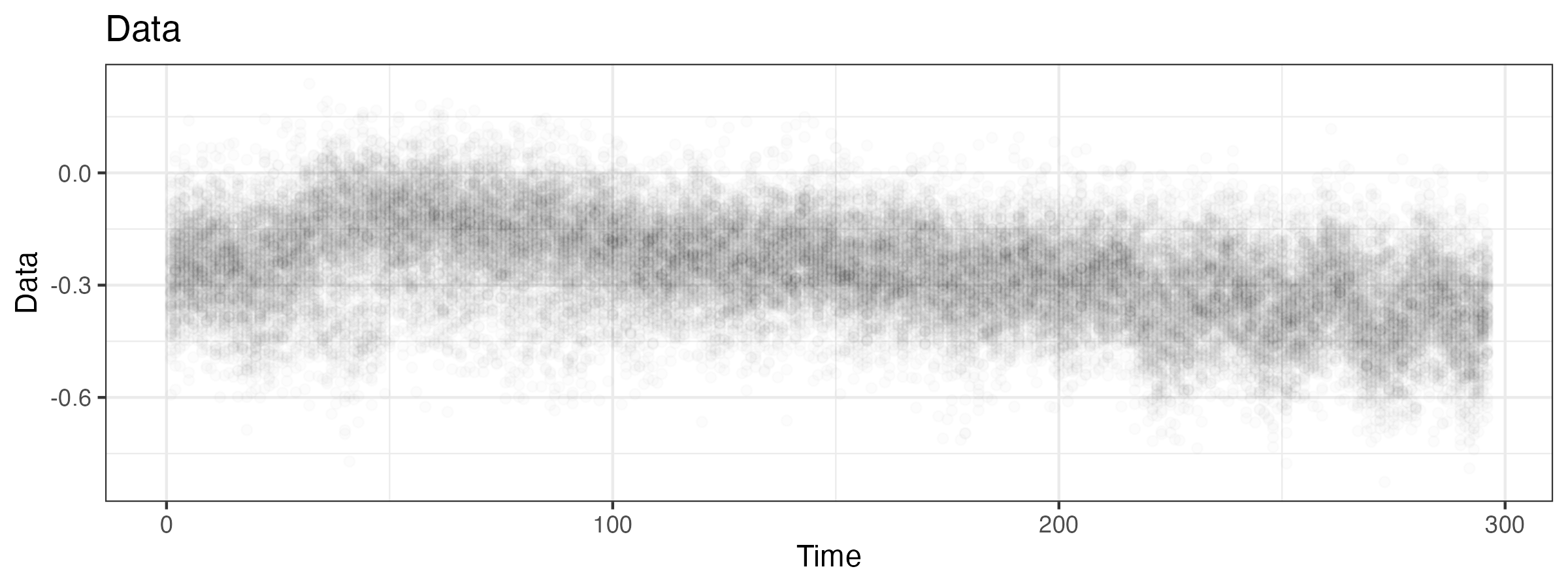
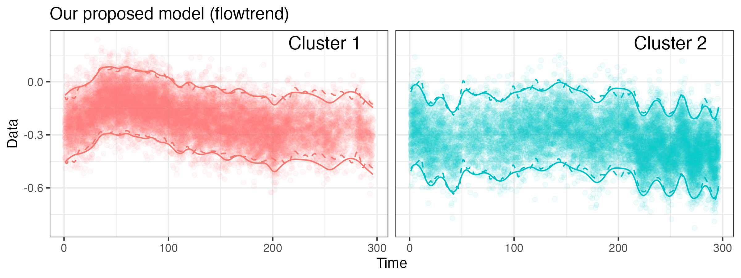
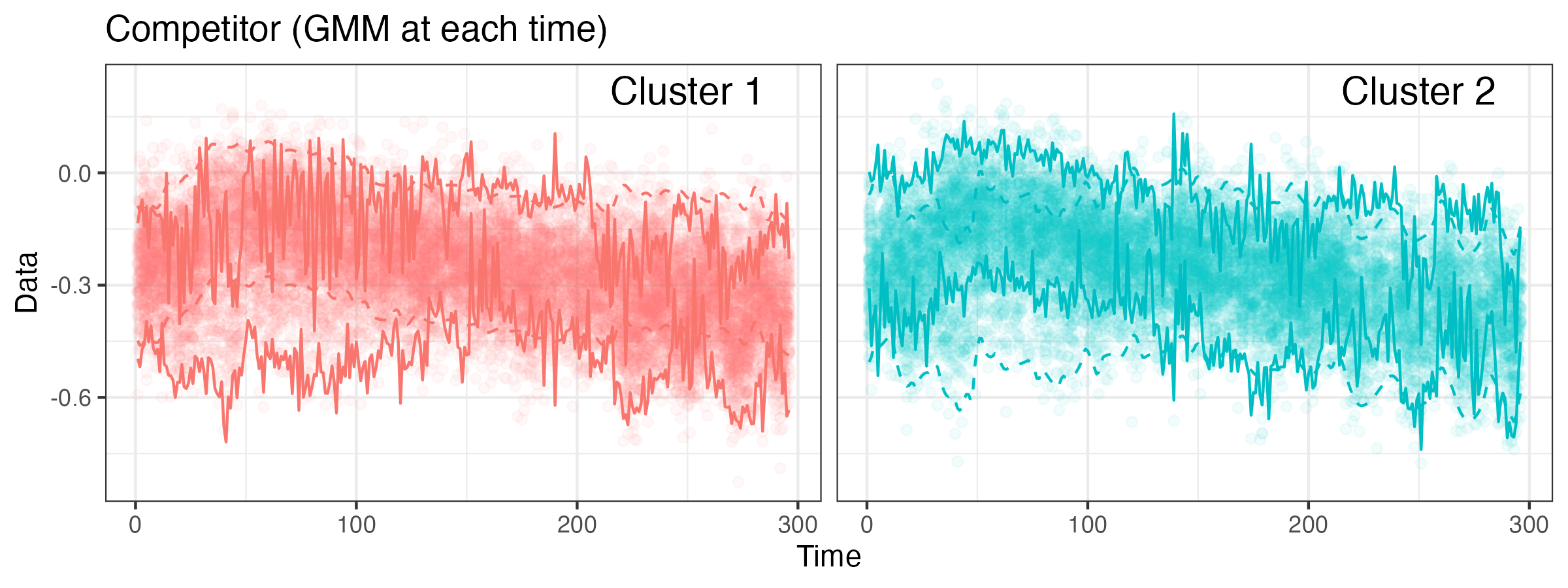
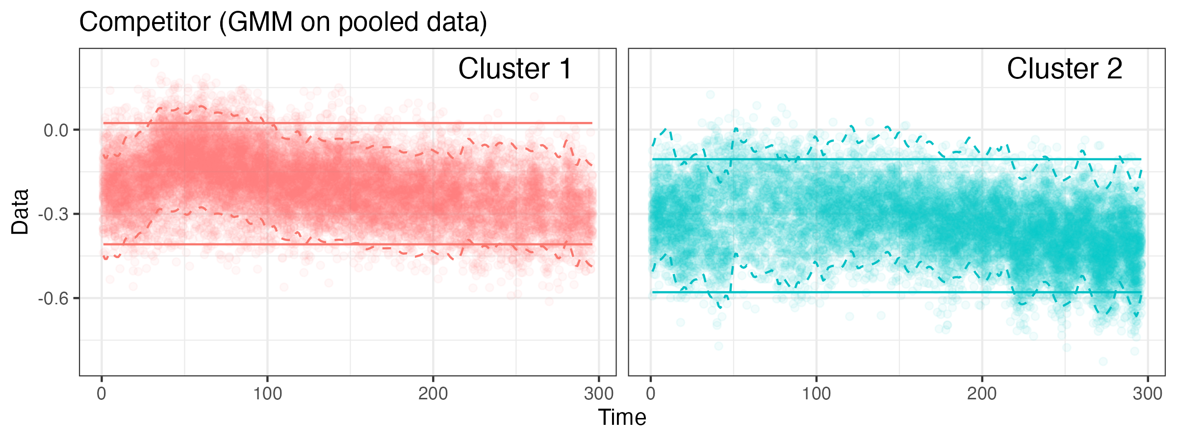
Figure 1: The top-left shows a pseudo-synthetic data example taken from a real dataset, for illustration. Every vertical slice is a time point $t=1,\cdots,T$, and the $y$ axis is the value of a particle in a 1-dimensional flow cytometry dataset of size $n_{t}=100$ at time $t$. There are two Gaussian clusters at each time point, and the parameters – means and probabilities – of each cluster are changing gradually over time. This is surprisingly hard to cluster accurately, and no tools are available for this problem. The first panel shows the data as-is. The remaining three panels show the result of “gating”, or clustering the particles into two groups. The dashed lines show the true 95% probability region for each cluster, and the solid lines show each model’s estimated 95% probability region from each cluster. The flowtrend model closely mimics the real model. The other two GMM-based baseline models are explained in Section LABEL:subsec:baseline_descrip, and the full simulation is shown in Section LABEL:sec:NumericExperiments.

The top-right panel of Figure 1 shows the result of applying the method that we propose in this paper, which we call flowtrend. We can see that it is able to estimate the true underlying model quite accurately. The key assumption made by flowtrend is that the data generating mechanism changes only gradually over time. Our method explicitly models the smoothly changing nature of a time series of mixtures by combining a nonparametric estimation technique with Gaussian mixture-of-experts modeling. In order to induce smoothness, we employ a trend-filtering model (steidl2006splines; kim2009ell_1; tibshirani2014adaptive) on the cluster means and probabilities across time. And from the estimated Gaussian mixture models, we can assign membership probabilities to each particle, which we can use for gating the particles.

The most similar method is the flowmix mixture-of-experts model (hyun2020modeling), which connects the time points directly by assuming the means and probabilities are regression functions of environmental covariates such as salinity, temperature or nutrients. Because many covariates are smooth across time, the means and probabilities are also estimated to be gradually varying across time. The major downside of flowmix is that this approach requires having environmental covariates at the analyst’s disposal, which is often not the case. Our proposed flowtrend model will be useful in the common setting that a scientist needs to perform gating but does not have access to relevant environmental covariates or does not want to assume a functional relationship between environment and cytograms.

Another method called CYBERTRACK (cybertrack) uses Gaussian mixtures to perform clustering for time-series flow cytometry data. However, CYBERTRACK only models the cluster probabilities $\pi$ over time as a stochastic process. Crucially, CYBERTRACK does not allow for means to be different across time. Our proposed flowtrend model is more appropriate for marine flow cytometry, where we know the cell populations’ optical properties shift and oscillate over time. Also, our model restricts the mean movement over time, which serves as implicit regularization of the cluster locations in their overall variation, thus allowing for a more direct biological interpretation of the estimated subpopulations.

There is a literature on mixture of regressions that is tangentially related. mixquantreg studies a semi-parametric mixture of quantile regressions model. Huang2013 considers a nonparametric mixture of regressions, but it is only designed for a univariate response and covariate pair and, furthermore, it is not designed for repeated responses. Xiang2019 provides a comprehensive overview of semi-parametric extensions of finite mixture models. xiangyao2017 proposes a related method using single-index models. All of these methods assume that covariates accompany a univariate, non-repeated mixture responses. Our proposed method and software is explicitly designed for multivariate and repeated responses that are gradually changing across time, without the need for accompanying covariates.

Accompanying this manuscript, we also publish an R package called flowtrend that implements our method and is designed to work on a multi-thread high-performance parallel computing system such as SLURM slurm. We used literate programming (Knuth1992-zz; litr) to write flowtrend, and the supplementary materials includes a bookdown (bookdown) which presents detailed explanations alongside the source code.

2 Methodology

In this section, we present our new method for modeling continuous flow cytometry data. The first three subsections introduce the three main components of the optimization problem we will be solving: the data generating model underlying our method (Section 2.1), the smoothness penalties which serve to regularize our estimates of the model parameters (Section 2.2), and the parameter constraints (Section 2.3). Section LABEL:subsec:Computation presents an expectation-maximization algorithm based on the optimization problem. Finally Sections LABEL:subsec:CV and LABEL:subsec:soft_gating describe how to select tuning parameters and use the model outputs in gating.

2.1 Basic model of cytogram data

The data we will model consist of an ordered sequence of $d$-dimensional scatterplots (which are referred to as “cytograms” hereafter). The cytogram at time $t$ consists of data points $y_{1}^{(t)},\ldots,y_{n_{t}}^{(t)}\in\mathbb{R}^{d}$, corresponding to the $n_{t}$ particles observed at time $t$. Across the $T$ time points, there are a total of $N=\sum_{t=1}^{T}n_{t}$ points. (For applications without repeated responses, we can simply set $n_{t}$ to $1$.) Our model assumes that each particle $y_{i}^{(t)}$ has a latent cluster membership $Z_{i}^{(t)}\in\{1,\cdots,K\}$, which will be thought of as the particle’s subtype. The $K$ subtype relative abundances vary with time (both due to the ship’s movement and due to the passage of time): $P(Z_{i}^{(t)}=k)=\pi_{kt}$. Given a latent membership $Z_{i}^{(t)}$, we model $y_{i}^{(t)}$ to be distributed as

$$Y_{i}^{(t)}|\{Z_{i}^{(t)}=k\}\sim\mathcal{N}_{d}\left(\mu_{kt\cdot},\Sigma_{k}\right).$$

Here, the vector $\mu_{kt\cdot}\in\mathbb{R}^{d}$ represents cell subtype $k$’s mean at time $t$, subsetted from $\mu\in\mathbb{R}^{K\times T\times d}$. Likewise, $\Sigma_{k}\in\mathbb{R}^{d\times d}$ is the $k$’th subtype’s variance-covariance. The choice to let the mean vary with time is based on the time-varying nature of the $d$ optical properties being captured by flow cytometry. For example, the diameter and chlorophyll concentration of cells are known to fluctuate on a daily cycle. Also, it is reasonable to assume the shape of the distribution of a subtype, encoded in $\Sigma_{k}$ does not change over time.

This mixture of Gaussians model has the following log-likelihood:

$$\ell\left(\{y_{i}^{(t)}\}_{i,t};\mu,\Sigma,\pi\right)=-\frac{1}{N}\sum_{t=1}^{T}\sum_{i=1}^{n_{t}}\log\left[\sum_{k=1}^{K}\pi_{kt}\cdot\phi\left(y_{i}^{(t)};\mu_{kt\cdot},\Sigma_{k}\right)\right],$$ (1)

where $\Sigma$ and $\pi$ written without subscripts denote the collections of parameters $\{\Sigma_{k}:1\leq k\leq K\}$, and $\{\pi_{kt}:1\leq k\leq K,1\leq t\leq T\}$, respectively.

The particles in ocean flow cytometry data often have accompanying biomass estimates. Small particles with small biomass are likely to be more numerous than large particles. Let us call $C_{i}^{(t)}$ the biomass of particle $y_{i}^{(t)}$. To account for the relative importance that a large particle should have in the data, we reweight the log-likelihood of $y_{i}^{(t)}$ by a factor of $C_{i}^{(t)}$ so that a modified pseudo-likelihood is:

$$\ell_{\text{biomass}}\left(\{{y_{i}^{(t)}}\}_{i,t},\{C_{i}^{(t)}\}_{i,t};\mu,\Sigma,\pi\right)=-\frac{1}{N}\sum_{t=1}^{T}\sum_{i=1}^{n_{t}}C_{i}^{(t)}\log\left[\sum_{k=1}^{K}\pi_{kt}\cdot\phi\left({y_{i}^{(t)}};\mu_{kt\cdot},\Sigma_{k}\right)\right],$$ (2)

where $N=\sum_{t=1}^{T}C_{i}^{(t)}$. Also, since cytograms often contain many points (with $n_{t}$ as large as $100,000$) computation can be challenging and compressing the data size by binning the particle-level cytogram data is convenient. We do this by discretizing the cytogram space into $B=D^{d}$ hyper-rectangles $\{E_{b}\}_{b=1}^{B}$, where $D$ is the number of discrete values in the grid along each axis, and recording the number of particles in each grid cell at each time point $t$ according to

$$C_{b}^{(t)}=\sum_{i=1}^{n_{t}}C_{i}^{(t)}\mathds{1}(y_{i}^{(t)}\in E_{b}),\ \text{for }b=1,...,B;t=1,...,T.$$

Let $\{y_{b}\}_{b=1}^{B}$ be the bin centers, and define $N=\sum_{b=1}^{B}\sum_{t=1}^{T}C_{b}^{(t)}$. From here, we can write the likelihood of the binned data,

$$\ell_{\text{binned}}\left(\{{y_{b}}\}_{b=1}^{B},\{C_{b}^{(t)}\}_{b=1}^{B};\mu,\Sigma,\pi\right)=-\frac{1}{N}\sum_{t=1}^{T}\sum_{b=1}^{B}C_{b}^{(t)}\log\left[\sum_{k=1}^{K}\pi_{kt}\cdot\phi\left(y_{b};\mu_{kt\cdot},\Sigma_{k}\right)\right].$$ (3)

To be clear, the pseudo-likelihoods (2) and (3) are a step removed from the data generating process of the data; however, this approach is useful in practice for lessening class imbalance and making computation more feasible, and it has been used before (hyun2020modeling). The computational advantage of (3) is sizeable since the computation of our model depends on the number of terms in the sum of the pseudolikelihood, and in general $N\gg T\cdot B$, which in turn can be much smaller than the number of nonempty bins, $\sum_{t=1}^{T}\sum_{b=1}^{B}\mathds{1}\{C_{b}>0\}$. Bin sparsity leads to considerable memory savings as well: for example, for a dataset with $T=296$ (considered in Section LABEL:sec:3dreal) the original particle-level data are several gigabytes whereas the binned data are in the tens of megabytes. Lastly, the expression in (2) is easily reduced to the true model when particles $y_{i}^{(t)}$ are observed without observation weights like biomass simply by taking $C_{i}^{(t)}=1$. We use the pseudolikelihood in (2) as the basis of the objective value to optimize for the rest of the paper because it subsumes (3) as a special case.

2.2 Trend filtering of each cluster’s $\mu$ and $\pi$

The basic model in Section 2.1 places no restrictions on $\mu_{kt\cdot}$ and $\pi_{kt}$, which allows them to be highly varying and choppy over time. On the other hand, it is apparent from plotting ocean flow cytometry data that the cell populations are slowly varying in time. In order to incorporate this knowledge while estimating model parameters $\mu_{kt\cdot}$ and $\pi_{kt}$, we make use of trend filtering, reviewed next.

Trend filtering (steidl2006splines; kim2009ell_1) is a tool for non-parametric regression on a sequence of output points $v=(v_{1},...,v_{T})$ observed at locations $x=(x_{1},...,x_{T})$. If $x$ is equally spaced, then the $l$-th order trend filtering estimate is obtained by solving

$$\min_{\psi\in\mathbb{R}^{T}}\frac{1}{2}\|v-\psi\|_{2}^{2}+\lambda\|D^{(l_{\mu}+1)}\psi\|_{1},$$

where $\lambda$ is a tuning parameter and $D^{(l_{\mu}+1)}\in\mathbb{R}^{(T-l-1)\times l}$ is the $(l_{\mu}+1)$-th order discrete differencing matrix defined recursively as $D^{(l+1)}=D^{(1)}D^{(l)}$, starting with $D^{(1)}\in\mathbb{R}^{(T-1)\times T}$:

$$D^{(1)}=\begin{bmatrix}-1&1&0&\cdots&0&0\\ 0&-1&1&\cdots&0&0\\ \vdots&&&&\\ 0&0&0&\cdots&-1&1\end{bmatrix}.$$

An order-$l$ trend filtering mean estimate is a piecewise polynomial of order $l$. For example, $l=0$ will produce a piecewise constant mean estimate $\hat{\mu}$. This special case is better known as the “fused lasso” (with no sparsity penalty, tibshirani2005sparsity) Likewise, $l=1$ will produce a piecewise linear estimate, while $l=2$ will produce a piecewise quadratic estimate. A straightforward change in $D^{(l)}$ allows for the input $x$ to be unevenly spaced (tibshirani2014adaptive, Section 6).

Porting these ideas to our problem, we add trend filtering penalties to encourage smoothness (with respect to time) in each $\mu_{k\cdot\cdot}\in\mathbb{R}^{T\times d}$ and $\pi_{k\cdot}\in\mathbb{R}^{T}$. For $\mu_{k\cdot\cdot}$, we use the penalty $\lambda_{\mu}\|D^{(l_{\mu}+1)}\mu_{k\cdot\cdot}\|_{1}$. Here, we use the notation that for a matrix $M$, $\|M\|_{1}=\|\text{vec}(M)\|_{1}$. For $\pi_{k\cdot}$, we apply the penalty on the scale of logits $\alpha_{kt}$ (denoting the $(k,t)$’th entry of $\alpha\in\mathbb{R}^{K\times T}$), where

$$\pi_{kt}=\frac{\exp(\alpha_{kt})}{\sum_{m=1}^{K}\exp(\alpha_{mt})}.$$ (4)

Putting this together, we aim to minimize the following penalized negative log-likelihood:

$$-\ell_{\text{biomass}}\left(\{{y_{i}^{(t)}}\}_{i,t},\{C_{i}^{(t)}\}_{i,t};\mu,\Sigma,\pi\right)+\lambda_{\mu}\sum_{k=1}^{K}\|D^{(l_{\mu}+1)}\mu_{k\cdot\cdot}\|_{1}+\lambda_{\pi}\sum_{k=1}^{K}\|D^{(l_{\pi}+1)}\alpha_{k\cdot}\|_{1},$$ (5)

where $\lambda_{\mu},\lambda_{\pi}$ are tuning parameters and $l_{\mu},l_{\pi}$ are the degree of trend filtering for $\{\mu_{kt\cdot}\}_{k,t}$ and $\{\pi_{kt}\}_{k,t}$ respectively.

2.3 Restricting mean movement

It is important in our application that each mean trajectory correspond consistently across all times to the same biological cell population. While the trend filtering penalties in the previous section help encourage this behavior, we wish to enforce this more directly. Cells from the same microbial type cannot change too much over time in their characteristics, being bound by the bio-physiological limits of a single subspecies.

We therefore add to (5) an explicit constraint, requiring that all the mean vectors for cluster $k$ across time, $\{\mu_{kt\cdot}:t=1,\ldots,T\}$, remain within a radius $r$ of their time average $\bar{\mu}^{(k)}=1/T\cdot\sum_{t=1}^{T}\mu_{kt\cdot}$:

μ, Σ, α

-1N∑_t=1^T∑_i=1^n_t C_i^(t)log[