On Resolution of $\ell_{1}$-norm minimization via a Two-metric Adaptive Projection Method

Abstract

The two-metric projection method is a simple yet elegant algorithm proposed by Bertsekas to address bound/box-constrained optimization problems. The algorithm’s low per-iteration cost and potential for using Hessian information make it a favorable computation method for this problem class. Inspired by this algorithm, we propose a two-metric adaptive projection method for solving the $\ell_{1}$-norm regularization problem that inherits these advantages. We demonstrate that the method is theoretically sound - it has global convergence. Furthermore, it is capable of manifold identification and has superlinear convergence rate under the error bound condition and strict complementarity. Therefore, given sparsity in the solution, the method enjoys superfast convergence in iteration while maintaining scalability, making it desirable for large-scale problems. We also equip the algorithm with competitive complexity to solve nonconvex problems. Numerical experiments are conducted to illustrate the advantages of this algorithm implied by the theory compared to other competitive methods, especially in large-scale scenarios. In contrast to the original two-metric projection method, our algorithm directly solves the $\ell_{1}$-norm minimization problem without resorting to the intermediate reformulation as a bound-constrained problem, so it circumvents the issue of numerical instability.

49M15, 49M37, 68Q25, 90C06, 90C25, 90C30

1 Introduction

In this paper, we consider the $\ell_{1}$-norm minimization problem:

(1) $$\min_{x\in\mathbb{R}^{n}}\psi(x)\triangleq f(x)+h(x),$$

where $f:\mathbb{R}^{n}\to\mathbb{R}$ is continuously differentiable, and $h(x)=\gamma\|x\|_{1}$.

The $\ell_{1}$-norm regularization is widely used in machine learning and statistics to promote sparsity in the solution. Many algorithms have been proposed to solve the $\ell_{1}$-norm regularization problem, such as the proximal gradient method [6], the accelerated proximal gradient method [18], the alternating direction method of multipliers (ADMM) [9], and the coordinate descent method [24]. However, these methods may converge slowly near the optimal point. Second-order methods are more desirable when seeking highly accurate solution. When $f$ is a twice continuously differentiable function, it is natural to expect algorithms to have faster convergence rates by exploiting the Hessian information of $f$ at each iterate $x_{k}$. Some successful algorithms have been proposed to solve the general composite optimization problem in the form of Eq. 1, such as the successive quadratic approximation (SQA) methods [30, 15], the semi-smooth Newton methods [14, 28] and the manifold optimization approach [3] based on the notion of partial smoothness [16].

In this work, we propose a two-metric adaptive projection method to address Eq. 1. The original two-metric projection method is proposed by Bertsekas [7, 12] to solve the bound constrained optimization problem:

(2) $$\begin{array}[]{rl}\min\;f(x)\quad\text{subject to}\;x\geq 0.\end{array}$$

Two-metric projection method is a simple yet elegant algorithm which can be descriced as follows:

(3) $$x_{k+1}=P(x_{k}-\alpha_{k}D_{k}\nabla f(x_{k})),$$

where $D_{k}$ is a positive definite matrix, and $P(\cdot)$ denotes the Euclidean projection onto the nonnegative orthant. Note that $P(\cdot)$ has a simple closed form: given any vector $v\in\mathbb{R}^{n}$, $i$th component of $P(v)$ is $\max\{v^{i},0\}$. Therefore, the method has a low per-iteration cost if $D_{k}$ is provided. When $D_{k}$ is constructed using the Hessian information, the algorithm potentially converges fast. However, Bertsekas pointed out an issue regarding Eq. 3: starting from the current iterate $x_{k}$, the objective function value may not decrease for any small stepsize $\alpha_{k}>0$ even when $D_{k}$ is chosen as inverse of the Hessian. This means that a naive projected Newton step may fail. To solve this issue, Bertsekas proposed to divide the index set into two parts in each iteration:

$$I_{k}^{+} =\{i\mid 0\leq x_{k}^{i}\leq\epsilon_{k},\nabla_{i}f(x_{k})>0\},$$

$$I_{k}^{-} =\{1,\ldots,d\}\setminus I_{k}^{+},$$

and choose $D_{k}$ such that it is diagonal regarding $I_{k}^{+}$, i.e.:

$$D_{k}[i,j]=0,\forall i,j\in I_{k}^{+}\mbox{ and }i\neq j.$$

The problem is fixed via this approach. Moreover, if the non-diagonal part of $D_{k}$ is constructed based on the Hessian inverse, it can be shown that under the assumption of second-order sufficient conditions and strict complementarity, the sequence of iterates identifies the manifold and is attracted to the local solution at a superlinear rate. Recently, the worst-case complexity property of the two-metric projection method in nonconvex setting has been studied in [27]: the algorithm can locate an $\epsilon$-approximate first-order optimal point in $\mathcal{O}(\epsilon^{-3})$ iterations. By properly scaling $D_{k}$, the complexity result is enhanced to $\mathcal{O}(\epsilon^{-2})$.

Note that the $\ell_{1}$-norm regularization problem is equivalent to a bound-constrained optimization problem when splitting $x$ into non-negative variables representing positive and negative components of $x$. Two-metric projection can be applied to this bound-constrained reformulation to resolve Eq. 1. Unfortunately, this approach may lead to numerical instability because the linear system may not have a solution when using Hessian inverse to build $D_{k}$ even if the Hessian of the original problem is positive-defnite [19]. Also note that global convergence and local superlinear convergence rate of the two-metric projection method require that the eigenvalues of $D_{k}$ are uniformly bounded (hence the sub-Hessian needs to be uniformly nonsingular), and the Newton system needs to be solved exactly. These requirements are rarely met in practice. One may also use (limited) BFGS to approximate the sub-Hessian as in [20] to build $D_{k}$. However, this will compromise the algorithm’s ability to find highly accurate solutions within reasonable time. Detailed discussion is in Section 6.

To avoid these issues, we propose a novel two-metric adaptive projection algorithm to solve Eq. 1. The algorithm is inspired by the two-metric projection method but directly solves Eq. 1 without resorting to the intermediate reformulation as a bound-constrained problem, so it circumvents the issue of numerical instability. Moreover, we do not require the Hessian to be uniformly positive definite nor solving the linear system exactly. Such design enables efficient and less stringent implementation to solve Eq. 1. Despite these improvements in numerical implementation, the algorithm preserves the identification of active set (optimal manifold) - it only needs to solve a low-dimensional linear system (Newton-equation) due to the sparsity structure of the optimal point. After manifold identification, it converges to the optimal solution in a superlinear rate. These convergence properties are shown using the strict complementarity and the error-bound condition that is weaker than the second-order sufficient condition and holds for a wide range of objective functions [32]. Our method is also favorable among the existing competitive second-order frameworks to solve Eq. 1. In particular, in each iteration we only need to solve a linear system of potentially low dimension inexactly, in sharp contrast to the proximal Newton methods [30, 15] which need to solve another $\ell_{1}$-norm regularized problem in full dimension at each step. Another method considered in [3] alternates between proximal gradient and Newton’s method to solve Eq. 1, aiming to use the former to identify the manifold and the latter to accelerate the convergence. The alternating design is necessary since they cannot know when a manifold is successfully identified. In contrast, our algorithm is able to identify the optimal manifold and reduce to a Newton’s method on the manifold automatically. These advantages are further verified via numerical experiments. We also explore the potential of this method to solve smooth nonconvex problems when the scaling matrix does not necessarily depend on Hessian. A competitve complexity close to the optimal $\mathcal{O}(\epsilon^{-2})$ is achieved after slight modification.

We summarize our contributions in this paper as follows:

1. We propose a novel two-metric adaptive projection algorithm for directly solving the $\ell_{1}$-norm minimization problem, which is easily implementable and has a low per-iteration cost.

2. We provide a comprehensive theoretical analysis of the proposed algorithm, including global convergence, manifold identification and local superlinear convergence rates under the error bound condition and strict complementarity.

3. We conduct numerical experiments on large-scale datasets to demonstrate the efficiency and effectiveness of our algorithm with comparison to other competitive methods.

4. We equip the algorithm with complexity guarantees close to the optimal when $f$ is smooth nonconvex.

The remainder of this paper is organized as follows: In Section 2 we clarify the basic assumptions and review the relevant background knowledge. In Section 3 the proposed algorithm is formally introduced in detail. Section 4 presents the theoretical analysis of the algorithm’s convergence properties. In Section 5 we discuss the experimental results. Discussion about the relationship between our algorithm and two-metric projection is included in Section 6, and we also illustrate in detail why we can not directly use the two-metric projection to solve the equivalent bound-constrained formulation of problem (1). Finally, in Section 7 we conclude the paper and discuss future work.

Notation

Suppose that $X^{*}$ denotes the optimal solution set of Eq. 1. $\|\cdot\|$ denotes the $\ell_{2}$-norm for vectors or operator norm for matrices. For a vector $v$ and index set $I$, let $v_{I}$ denote the subvector of $v$ w.r.t. $I$ and $v^{i}$ denote the $i$th component of $v$. For any point $x$ and set $S$, let ${\rm dist}(x,S)\triangleq\inf\{\|x-y\|\mid y\in S\}$. For a convex function $f:\mathbb{R}^{b}\to\mathbb{R}$, $\partial f$ denotes its subdifferential set, i.e., $\partial f(x)\triangleq\{g\mid f(y)\geq f(x)+g^{T}(y-x),\;\forall y\in\mathbb{R}^{b}\}$. For a smooth function $f$ on $\mathbb{R}^{n}$, $\nabla f$ and $\nabla^{2}f$ denote its Euclidean gradient and Euclidean Hessian, respectively. For a smooth function $f$ on a manifold $\mathcal{M}$, $\operatorname{grad}_{\mathcal{M}}f$ and $\operatorname{Hess}_{\mathcal{M}}f$ denote its Riemannian gradient and Riemannian Hessian, respectively.

2 Preliminaries

2.1 Nonsmooth optimization

Optimality conditions and critical points

If $x^{*}$ is an optimal point of $\ell_{1}$-norm minimization problem Eq. 1 then,

(4) $$-\nabla f\left(x^{*}\right)\in\gamma\partial\left\|x^{*}\right\|_{1}$$

(c.f. [2]). Specifically, Eq. 4 is equivalent to

(5) $$\nabla_{i}f\left(x^{*}\right)=\left\{\begin{array}[]{ll}-\gamma,&(x^{*})^{i}>0,\\ a\in[-\gamma,\gamma],&(x^{*})^{i}=0,\\ \gamma,&(x^{*})^{i}<0.\end{array}\right.$$

Remark 2.1.

When $f$ is a convex function, the necessary optimality condition (4) is also sufficient.

Proximity operator

For a convex function $h$, proximity operator is defined as the set-valued mapping

$$\operatorname{prox}_{h}(x)=\underset{u\in\operatorname{dom}h}{\arg\min}\left\{h(u)+\frac{1}{2}\|u-x\|^{2}\right\}.$$

If $h$ is a proper lower semicontinuous convex function, then $\operatorname{prox}_{h}(x)$ uniquely attained (c.f. [4]).

Relation between proximity operator and optimality conditions

If $x^{*}$ satisfies the first-order necessary conditions Eq. 5, we say that $x^{*}$ is a critical (stationary) point of Eq. 1. In particular, $x^{*}$ is critical iff

(6) $$x^{*}=\operatorname{prox}_{\alpha h}(x^{*}-\alpha\nabla f(x^{*}))$$

for any $\alpha>0$.

2.2 Riemannian optimization

Definition 2.2 (Fixed coordinate-sparsity subspaces).

$$\mathcal{M}_{I}\triangleq\left\{x\in\mathbb{R}^{n}:x^{i}=0\text{ for }i\in I\right\},$$

where $I$ is an index set.

For such $\mathcal{M}_{I}$, $T_{x}\mathcal{M}_{I}$ denotes the tangent space of $\mathcal{M}_{I}$ at $x$ and $\mathrm{T}\mathcal{M}_{I}$ denotes the tangent bundle. Then we have

$$T_{x}\mathcal{M}_{I}=\mathcal{M}_{I}.$$

For $(x,\eta)\in\mathrm{T}\mathcal{M}_{I}$, Riemannian gradient and Hessian of function $F$ smooth at $x\in\mathcal{M}_{I}$ can be written as follows,

$$\operatorname{grad}_{\mathcal{M}_{I}}F(x)=\operatorname{proj}_{x}(\nabla F(x)),$$

$$\operatorname{Hess}_{\mathcal{M}_{I}}F(x)[\eta]=\operatorname{proj}_{x}\left(\nabla^{2}F(x)\eta\right),$$

where $\operatorname{proj}_{x}$ is the Euclidean projection onto $T_{x}\mathcal{M}_{I}$. A second-order retraction in this case is as follows,

$$\mathrm{R}_{x}(\eta)=x+\eta.$$

More details about Riemannian optimization can be found in [1, 8]. Next we define the active set of a point $x$ for problem Eq. 1.

Definition 2.3 (Active set).

For any $x\in\mathbb{R}^{n}$, define

$$\mathcal{A}(x)\triangleq\left\{i\mid x^{i}=0\right\}.$$

Then, the optimal manifold associated with $x^{*}$ is defined as $\mathcal{M}_{*}\triangleq\mathcal{M}_{\mathcal{A}(x^{*})}$, where $x^{*}$ is an optimal point of problem Eq. 1. Note that $\mathcal{M}_{*}$ is an embedded submanifold of $\mathbb{R}^{n}$, and the Riemannian metric is same as the Euclidean metric. It is worth noting that $\psi(x)$ may not be smooth around $x^{*}$ in $\mathbb{R}^{n}$, but it is locally smooth around $x^{*}$ on $\mathcal{M}_{*}$. Next we introduce a lemma useful in our later proofs.

Lemma 2.4 ([8]).

If $f:\mathcal{M}\rightarrow\mathbb{R}$ has Lipschitz continuous Hessian, then there exists $L_{H}>0$ such that

(7) $$\left|f\left(\operatorname{Exp}_{x}(s)\right)-f(x)-\langle s,\operatorname{grad}f(x)\rangle-\frac{1}{2}\langle s,\operatorname{Hess}f(x)[s]\rangle\right|\leq\frac{L_{H}}{6}\|s\|^{3}$$

and

(8) $$\left\|P_{s}^{-1}\operatorname{grad}f\left(\operatorname{Exp}_{x}(s)\right)-\operatorname{grad}f(x)-\operatorname{Hess}f(x)[s]\right\|\leq\frac{L_{H}}{2}\|s\|^{2}$$

for all $(x,s)$ in the domain of the exponential map $\operatorname{Exp}$ and $P_{s}$ denotes parallel transport along $\gamma(t)=\operatorname{Exp}_{x}(ts)$ from $t=0$ to $t=1$.

2.3 Basic assumptions

The following assumption will be used throughout the paper.

Assumption 2.5.

Suppose that the following hold:

1. $f$ is continuously differentiable with an $L_{g}$-Lipschitz continuous gradient;

2. $\psi(x)$ is bounded below by $\underline{\psi}$;

3. $\psi(x)$ has bounded sublevel set.

Remark 2.6.

$\psi=f+h$ is also lower semi-continuous therefore every sublevel set $\mathcal{L}_{\psi}\left(x_{0}\right)\triangleq\{x\mid\psi(x)\leq\alpha\}$ is closed thus compact. Therefore, $X^{*}$ is also compact.

Assumption 2.7 - 2.12 will be used in the local convergence rate analysis.

Assumption 2.7 (Strict complementarity or SC).

$x$ is a critical point that satisfies the strict complementarity condition if

$$0\in\operatorname{relint}(\nabla f(x)+\partial h(x)).$$

Assumption 2.8 (Error bound or EB).

For an optimal point $x^{*}\in X^{*}$, there exists a neighborhood $B\left(x^{*},b_{1}\right)$ such that for all $x\in B\left(x^{*},b_{1}\right)$,

$$c_{1}\|x-\operatorname{prox}_{h}(x-\nabla f(x))\|\geq\operatorname{dist}\left(x,X^{*}\right)$$

Assumption 2.9 (Error bound on Manifold).

For an optimal point $x^{*}\in X^{*}$, there exists $b_{1}>0$ such that for all $x\in\mathcal{M}_{*}\cap B\left(x^{*},b_{1}\right)$

$$c_{1}\|\operatorname{grad}_{\mathcal{M}_{*}}\psi(x)\|\geq\operatorname{dist}\left(x,X^{*}\cap\mathcal{M}_{*}\right).$$

We illustrate the relationship between 2.8 and 2.9 via the following Theorem.

Theorem 2.10.

When SC holds at an optimal point $x^{*}$,2.8 implies 2.9.

Proof 2.11.

Since $x^{*}$ satisfies SC, there exists a neighborhood $B\left(x^{*},2b_{1}\right)$ (w.l.o.g we suppose $b_{1}$ is same as 2.8) such that for all $x\in B\left(x^{*},2b_{1}\right)\cap X^{*}\subseteq\mathcal{M}_{*}$. Define $\Pi_{X^{*}}(x)\triangleq\operatorname{argmin}_{y\in X^{*}}\|y-x\|$, and let $\tilde{x}=\Pi_{X^{*}}(x)$. Then we have for all $x\in B\left(x^{*},b_{1}\right)$

$$\|x-\tilde{x}\|=\operatorname{dist}\left(x,X^{*}\right)\leq\|x-x^{*}\|<b_{1}$$

Therefore, $\|\tilde{x}-x^{*}\|\leq\|x-\tilde{x}\|+\|x-x^{*}\|<2b_{1}$ and $\tilde{x}\in\mathcal{M}_{*}$. Since

$$\|x-\tilde{x}\|=\operatorname{dist}\left(x,X^{*}\right)\leq\operatorname{dist}\left(x,X^{*}\cap\mathcal{M}_{*}\right)\leq\|x-\tilde{x}\|$$

which means that $\operatorname{dist}\left(x,X^{*}\right)=\operatorname{dist}\left(x,X^{*}\cap\mathcal{M}_{*}\right)$. If $x\in\mathcal{M}_{*}$, then with a small neighborhood of $x^{*}$, we have

$$\|x-\operatorname{prox}_{h}(x-\nabla f(x))\|=\|\operatorname{grad}_{\mathcal{M}_{*}}\psi(x)\|$$

by SC and continuity (w.l.o.g. suppose this neighborhood is also $B\left(x^{*},b_{1}\right)$).

Assumption 2.12 (Lipschitz Hessian).

For an optimal point $x^{*}$, there exists $b_{2}>0$ such that $\operatorname{Hess}_{\mathcal{M}_{*}}f$ is Lipschitz continuous in $B\left(x^{*},b_{2}\right)$ on $\mathcal{M}_{*}$.

Remark 2.13.

2.7 is a common assumption in literature [13, 23] to guarantee manifold identification. 2.8 is a local condition that is weaker than local strong convexity and sufficient second-order condition [14]. It has been shown to hold for a general class of structured convex optimization problems including the $\ell_{1}$-norm regularized logistic regression and least squares [32]. 2.12 is also mild and holds when $\nabla^{2}f$ is Lipschitz continuous around $x^{*}$.

3 Two-metric Adaptive Projection Algorithm

Now we describe the two-metric adaptive projection algorithm for finding the critical point $x^{*}$ of Eq. 1. Analogously, we partition the index set into $I_{k}^{+}$ and $I_{k}^{-}$, and scale the gradient component in these two parts differently. In addition, the $I_{k}^{-}$ part needs to be further split to deal with the singularity of $|\cdot|$ at $0$. Definition of the projection operator depends on the current iterate, hence the name “adative projection”. Specifically, given $x_{k}\in\mathbb{R}^{n}$, accuracy level $\epsilon>0$, denote

$$\pi_{k}\triangleq\|x_{k}-\operatorname{prox}_{h}(x_{k}-\nabla f(x_{k}))\|\text{ and }\epsilon_{k}\triangleq\min\{\epsilon,\pi_{k}\}.$$

Let $g_{k}\triangleq\nabla f\left(x_{k}\right)$. Partition the index set as follows: $\{1,...,n\}=I_{k}^{+}\cup I_{k}^{-+}\cup I_{k}^{--}$, and

$$I_{k}^{+} \triangleq\left\{i:\begin{array}[]{l}|x_{k}^{i}|\leq\epsilon_{k},|g_{k}^{i}|<\gamma\;\mbox{or}\\ -\epsilon_{k}\leq x_{k}^{i}<0,g_{k}^{i}\leq-\gamma\;\mbox{or}\\ 0<x_{k}^{i}\leq\epsilon_{k},g_{k}^{i}\geq\gamma\end{array}\right\},$$

$$I_{k}^{-+} \triangleq\left\{i:\begin{array}[]{l}x_{k}^{i}>\epsilon_{k}\mbox{ or}\\ 0\leq x_{k}^{i}\leq\epsilon_{k},g_{k}^{i}\leq-\gamma\end{array}\right\},$$

$$I_{k}^{--} \triangleq\left\{i:\begin{array}[]{l}x_{k}^{i}<-\epsilon_{k}\mbox{ or}\\ -\epsilon_{k}\leq x_{k}^{i}\leq 0,g_{k}^{i}\geq\gamma\end{array}\right\},$$

$$I_{k}^{-} \triangleq I_{k}^{-+}\cup I_{k}^{--}.$$

We update $x_{k+1}$ via the following fomula:

$$x_{k+1}:=\mathcal{P}_{k,\epsilon}\left(x_{k}-t_{k}p_{k}\right),\quad\forall k\geq 0,$$

where $t_{k}>0$ is the stepsize. The step $p_{k}$ is defined as below:

$$[p_{k}]_{I_{k}^{+}}\triangleq[g_{k}+\omega_{k,\epsilon}]_{I_{k}^{+}}$$

and $[p_{k}]_{I_{k}^{-}}$ satisfies

(9) $$(H_{k}+\mu_{k}I)[p_{k}]_{I_{k}^{-}}=[g_{k}+\omega_{k,\epsilon}]_{I_{k}^{-}}+r_{k}$$

where $H_{k}$ is a symmetric positive semi-definite matrix and suppose $\|H_{k}\|\leq\lambda_{\max},\forall k$, $\mu_{k}$ is a positive scalar such that

$$\mu_{k}=c\left\|\begin{bmatrix}[x_{k}-\operatorname{Prox}_{h}(x_{k}-g_{k})]_{I_{k}^{+}}\\ [g_{k}+\omega_{k}]_{I_{k}^{-}}\end{bmatrix}\right\|^{\delta},\delta\in(0,1),$$

and $r_{k}\in\mathbb{R}^{|I_{k}^{-}|}$ is a residual that satisfies the following condition for a fixed $\tau\in(0,1)$:

(10) $$\|r_{k}\|\leq\tau\min\{\mu_{k}\|\bar{p}_{k}\|,\|\bar{g}_{k}+\bar{\omega}_{k,\omega}\|\}.$$

$\mathcal{P}_{k,\epsilon}$ and $\omega_{k,\epsilon}$ are associated to $x_{k},\epsilon$ and defined as below (recall that $S_{t}$ denotes the soft thresholding operator):

$$\mathcal{P}_{k,\epsilon}^{i}(v)=\begin{cases}\max\left\{v^{i},0\right\}&\text{ if }i\in I_{k}^{-+}\\ \min\left\{v^{i},0\right\}&\text{ if }i\in I_{k}^{--}\\ S_{t_{k}\gamma}(v^{i})&\text{ if }i\in I_{k}^{+}\end{cases}$$

$$\omega_{k,\epsilon}^{i}=\begin{cases}\gamma&\quad\text{ if }i\in I_{k}^{-+}\\ -\gamma&\quad\text{ if }i\in I_{k}^{--}\\ 0&\quad\text{ if }i\in I_{k}^{+}\end{cases}.$$

Suppose that

$$x_{k}(t)\triangleq\mathcal{P}_{k,\epsilon}\left(x_{k}-tp_{k}\right),\forall t>0.$$

Let $\bar{g}_{k}$, $\bar{p}_{k}$ and $\bar{\omega}_{k,\epsilon}$ be the subvectors of $g_{k}$, $p_{k}$ and $\omega_{k,\epsilon}$ w.r.t index set $I_{k}^{-}$. Let $x_{k}^{+}$, $x_{k}^{+}(t)$, $g_{k}^{+}$ be the subvector of $x_{k}$, $x_{k}(t)$, $g_{k}$ w.r.t index set $I_{k}^{+}$, respectively. Define $h_{k}^{+}(y)\triangleq\gamma{\bf 1}^{T}|y|$, where $y\in\mathbb{R}^{|I_{k}^{+}|}$ and we apply $|\cdot|$ to $y$ component-wisely.

The gradient map at iteration $k$ is defined as follows:

(11) $$G_{t}^{k}(x_{k}^{+})=\frac{x_{k}^{+}-\operatorname{prox}_{th_{k}^{+}}(x_{k}^{+}-tg_{k}^{+})}{t}=\frac{x_{k}^{+}-x_{k}^{+}(t)}{t}.$$

Then the algorithm can be formally stated as follows.

Algorithm 1 Two-metric Adaptive Projection Algorithm

 Input: accuracy level $\epsilon>0$, step acceptance parameter $\sigma\in(0,1)$, backtracking parameter $\beta\in(0,1)$, parameter $\tau\in(0,1)$ and initial point $x_{0}$.

 for $k=0,1,\ldots,$ do

  Let $t_{k}=1$

  if $\psi\left(x_{k}\right)-\psi\left(x_{k}\left(t_{k}\right)\right)<\sigma t_{k}(1-\tau)\mu_{k}\|\bar{p}_{k}\|^{2}+\sigma t_{k}\|G_{t_{k}}^{k}(x_{k}^{+})\|^{2}$ then

   $t_{k}=\beta t_{k}$

  else

   break

  end if

  $x_{k+1}=x_{k}\left(t_{k}\right)$

 end for

4 Convergence property

In this section, we discuss the theoretical guarantees/advantages of Algorithm 1. These results demonstrate its correctness and provide perspectives of why it works well in practice.

First of all, we need to show that the algorithm is well-defined. Specifically, we need to show that the backtracking linesearch (inner loop of Algorithm 1) can stop. We begin with the following two lemmas which hold under 2.5.

Lemma 4.1.

If $t\leq\frac{2(1-\sigma)}{L_{g}}$, we have

$$\psi(x_{k}(t))-\psi(x_{k})\leq\sum_{i\in I_{k}^{-}}\left((g_{k}^{i}+\omega_{k,\epsilon}^{i})(x_{k}^{i}(t)-x_{k}^{i})+\frac{L_{g}}{2}(x_{k}^{i}(t)-x_{k}^{i})^{2}\right)-\sigma t\|G^{k}_{t}(x_{k}^{+})\|_{2}^{2}.$$

Proof 4.2.

According to Eq. 11, we have

$$x_{k}^{+}(t)=\operatorname{prox}_{th_{k}^{+}}(x_{k}^{+}-tg_{k}^{+})=x_{k}^{+}-tG_{t}^{k}(x_{k}^{+}).$$

Then by the definition of proximal operator, we have

$$0\in x_{k}^{+}(t)-(x_{k}^{+}-tg_{k}^{+})+t\partial h_{k}^{+}(x_{k}^{+}(t))$$

(12) $$\implies G_{t}^{k}(x_{k}^{+})-g_{k}^{+}\in\partial h_{k}^{+}(x_{k}^{+}(t)).$$

Without loss of generality, we assume that

$$I_{k}^{+} =\left\{1,2,\ldots,n_{1}\right\},$$

$$I_{k}^{-+} =\left\{n_{1}+1,\ldots,n_{2}\right\},$$

$$I_{k}^{--} =\left\{n_{2}+1,\ldots,n\right\}.$$

Therefore, by $h(x_{k}(t))=h_{k}^{+}(x_{k}^{+}(t))+\gamma\sum_{i\in I_{k}^{-+}}|x_{k}^{i}(t)|+\gamma\sum_{i\in I_{k}^{--}}|x_{k}^{i}(t)|$ and the fact that for any $i\in I_{k}^{-+}$, $x^{i}_{k}(t)\geq 0$ and for any $i\in I_{k}^{--}$, $x^{i}_{k}(t)\leq 0$, we have

$$\begin{pmatrix}G^{k}_{t}(x_{k}^{+})-g_{k}^{+}\\ \gamma\\ \vdots\\ \gamma\\ -\gamma\\ \vdots\\ -\gamma\end{pmatrix}\in\partial h(x_{k}(t))$$

Since $h(x)$ is convex, then

(13) $$h(x_{k})\geq h(x_{k}(t))+\left(G^{k}_{t}(x_{k}^{+})-g_{k}^{+}\right)^{T}tG_{t}^{k}(x_{k}^{+})+\gamma\sum_{i\in I_{k}^{-+}}(x_{k}^{i}-x_{k}^{i}(t))-\gamma\sum_{i\in I_{k}^{--}}(x_{k}^{i}-x_{k}^{i}(t))$$

Therefore, by Lipschitz continuity of $f$ and Eq. 13, we have

$$\psi(x_{k}(t)) =f(x_{k}(t))+h(x_{k}(t))$$

$$\leq f(x_{k})+h(x_{k})+g_{k}^{T}(x_{k}(t)-x_{k})+\frac{L_{g}}{2}\|x_{k}(t)-x_{k}\|^{2}$$

$$+\left(g_{k}^{+}-G^{k}_{t}(x_{k}^{+})\right)^{T}tG_{t}^{k}(x_{k}^{+})-\gamma\sum_{i\in I_{k}^{-+}}(x_{k}^{i}-x_{k}^{i}(t))+\gamma\sum_{i\in I_{k}^{--}}(x_{k}^{i}-x_{k}^{i}(t))$$

$$\leq\psi(x_{k})-t(G_{t}^{k}(x_{k}^{+}))^{T}G_{t}^{k}(x_{k}^{+})+\frac{L_{g}t^{2}}{2}\|G_{t}^{k}(x_{k}^{+})\|_{2}^{2}$$

$$+\sum_{i\in I_{k}^{-}}\left((g_{k}^{i}+\omega_{k,\epsilon}^{i})(x_{k}^{i}(t)-x_{k}^{i})+\frac{L_{g}}{2}(x_{k}^{i}(t)-x_{k}^{i})^{2}\right)$$

$$=\psi(x_{k})+\left(\frac{L_{g}t^{2}}{2}-t\right)\|G^{k}_{t}(x_{k}^{+})\|_{2}^{2}$$

$$+\sum_{i\in I_{k}^{-}}\left((g_{k}^{i}+\omega_{k,\epsilon}^{i})(x_{k}^{i}(t)-x_{k}^{i})+\frac{L_{g}}{2}(x_{k}^{i}(t)-x_{k}^{i})^{2}\right).$$

If $t\leq\frac{2(1-\sigma)}{L_{g}}$, then

$$\psi(x_{k}(t))-\psi(x_{k})\leq\sum_{i\in I_{k}^{-}}\left((g_{k}^{i}+\omega_{k,\epsilon}^{i})(x_{k}^{i}(t)-x_{k}^{i})+\frac{L_{g}}{2}(x_{k}^{i}(t)-x_{k}^{i})^{2}\right)-\sigma t\|G^{k}_{t}(x_{k}^{+})\|_{2}^{2}.$$

This concludes the proof.

We assume that ${g_{k}}$ is bounded without loss of generality and will demonstrate this in Remark 4.6 after Theorem 4.5. Note that

$$\|\bar{p}_{k}\| =\|(H_{k}+\mu_{k}I)^{-1}(\bar{g}_{k}+\bar{\omega}_{k,\epsilon}+r_{k})\|$$

$$\leq\mu_{k}^{-1}(\|\bar{g}_{k}+\bar{\omega}_{k,\epsilon}\|+\|r_{k}\|)$$

$$\leq c^{-1}\|\bar{g}_{k}+\bar{\omega}_{k,\epsilon}\|^{1-\delta}+\tau\|\bar{p}_{k}\|$$

which indicates that

(14) $$\|\bar{p}_{k}\|\leq\frac{c^{-1}\|\bar{g}_{k}+\bar{\omega}_{k,\epsilon}\|^{1-\delta}}{1-\tau}.$$

Therefore, we let $G$ be a constant such that for any $k$,

(15) $$\|\bar{p}_{k}\|\leq G.$$

Lemma 4.3.

If $t$ satisfies

$$t\leq\min\left(\frac{2(1-\sigma)(1-\tau)\mu_{k}}{L_{g}},\frac{\epsilon_{k}}{G}\right)$$

then we have:

$$\sum_{i\in I_{k}^{-}}\left((g_{k}^{i}+\omega_{k,\epsilon}^{i})(x_{k}^{i}(t)-x_{k}^{i})+\frac{L_{g}}{2}(x_{k}^{i}(t)-x_{k}^{i})^{2}\right)\leq-\sigma t(1-\tau)\mu_{k}\|\bar{p}_{k}\|^{2}.$$

Proof 4.4.

If $x_{k}$ is critical, the result is immediate. Now suppose that $x_{k}$ is not critical. Then $\epsilon_{k}>0$.
Case 1: For $x_{k}^{i}>\epsilon_{k}$ or $x_{k}^{i}<-\epsilon_{k}$, we have

$$x_{k}^{i}(t)=x_{k}^{i}-tp_{k}^{i},\quad\text{if }t\leq\frac{\epsilon_{k}}{G}.$$

Therefore,

$$(g_{k}^{i}+\omega_{k,\epsilon}^{i})(x_{k}^{i}(t)-x_{k}^{i})+\frac{L_{g}}{2}(x_{k}^{i}(t)-x_{k}^{i})^{2}=\frac{L_{g}}{2}(tp_{k}^{i})^{2}-(g_{k}^{i}+\omega_{k,\epsilon}^{i})(tp_{k}^{i}).$$

Case 2: For $0\leq x_{k}^{i}\leq\epsilon_{k},g_{k}^{i}\leq-\gamma$

$$x_{k}^{i}(t)\geq x_{k}^{i}-tp_{k}^{i}\Longrightarrow(g_{k}^{i}+\omega_{k,\epsilon}^{i})(x_{k}^{i}(t)-x_{k}^{i})\leq-tp_{k}^{i}(g_{k}^{i}+\omega_{k,\epsilon}^{i}).$$

Since $x_{k}^{i}\geq 0$, we also have

$$\frac{L_{g}}{2}(x_{k}^{i}(t)-x_{k}^{i})^{2}\leq\frac{L_{g}}{2}(tp_{k}^{i})^{2}.$$

Therefore, in this case

$$(g_{k}^{i}+\omega_{k,\epsilon}^{i})(x_{k}^{i}(t)-x_{k}^{i})+\frac{L_{g}}{2}(x_{k}^{i}(t)-x_{k}^{i})^{2}\leq\frac{L_{g}}{2}(tp_{k}^{i})^{2}-(g_{k}^{i}+\omega_{k,\epsilon}^{i})(tp_{k}^{i}).$$

Case 3: For $-\epsilon_{k}\leq x_{k}^{i}\leq 0,g_{k}^{i}\geq\gamma$ we can do the similar step like above and we will have

$$(g_{k}^{i}+\omega_{k,\epsilon}^{i})(x_{k}^{i}(t)-x_{k}^{i})+\frac{L_{g}}{2}(x_{k}^{i}(t)-x_{k}^{i})^{2}\leq\frac{L_{g}}{2}(tp_{k}^{i})^{2}-(g_{k}^{i}+\omega_{k,\epsilon}^{i})(tp_{k}^{i}).$$

To conclude, for $i\in I_{k}^{-}$ we have,

$$(g_{k}^{i}+\omega_{k,\epsilon}^{i})(x_{k}^{i}(t)-x_{k}^{i})+\frac{L_{g}}{2}(x_{k}^{i}(t)-x_{k}^{i})^{2}\leq\frac{L_{g}}{2}(tp_{k}^{i})^{2}-(g_{k}^{i}+\omega_{k,\epsilon}^{i})(tp_{k}^{i}),$$

i.e.,

$$\sum_{i\in I_{k}^{-}}\left((g_{k}^{i}+\omega_{k,\epsilon}^{i})(x_{k}^{i}(t)-x_{k}^{i})+\frac{L_{g}}{2}(x_{k}^{i}(t)-x_{k}^{i})^{2}\right)\leq\frac{L_{g}}{2}t^{2}\|\bar{p}_{k}\|^{2}-t(\bar{g}_{k}+\bar{\omega}_{k,\epsilon})^{T}\bar{p}_{k}$$

We consider $(\bar{g}_{k}+\bar{\omega}_{k,\epsilon})^{T}\bar{p}_{k}$,

$$(\bar{g}_{k}+\bar{\omega}_{k,\epsilon})^{T}\bar{p}_{k} =\bar{p}_{k}^{T}(H_{k}+\mu_{k}I)\bar{p}_{k}-\bar{p}_{k}^{T}r_{k}$$

$$\geq\mu_{k}\|\bar{p}_{k}\|^{2}-\|\bar{p}_{k}\|\|r_{k}\|$$

$$\geq\mu_{k}\|\bar{p}_{k}\|^{2}-\tau\mu_{k}\|\bar{p}_{k}\|^{2}$$

$$=(1-\tau)\mu_{k}\|\bar{p}_{k}\|^{2}$$

Therefore,

$$\sum_{i\in I_{k}^{-}}\left((g_{k}^{i}+\omega_{k,\epsilon}^{i})(x_{k}^{i}(t)-x_{k}^{i})+\frac{L_{g}}{2}(x_{k}^{i}(t)-x_{k}^{i})^{2}\right)\leq\frac{L_{g}}{2}t^{2}\|\bar{p}_{k}\|^{2}-t(1-\tau)\mu_{k}\|\bar{p}_{k}\|^{2}.$$

When $t\leq\frac{2(1-\sigma)(1-\tau)\mu_{k}}{L_{g}}$,

$$\frac{L_{g}}{2}t^{2}\|\bar{p}_{k}\|^{2}-t(1-\tau)\mu_{k}\|\bar{p}_{k}\|^{2}=t\left(\frac{L_{g}}{2}t-(1-\tau)\mu_{k}\right)\|\bar{p}_{k}\|^{2}\leq-\sigma t(1-\tau)\mu_{k}\|\bar{p}_{k}\|^{2}.$$

This concludes the proof.

These two lemmas immediately indicates the following. The result of Theorem 4.5 guarantees that the linesearch in the inner loop of Algorithm 1 is well-defined.

Theorem 4.5.

Suppose that 2.5 holds. Then if

$$t\leq\min\left(\frac{2(1-\sigma)}{L_{g}},\frac{2(1-\sigma)(1-\tau)\mu_{k}}{L_{g}},\frac{\epsilon_{k}}{G}\right),$$

we have

(16) $$\psi\left(x_{k}\right)-\psi\left(x_{k}\left(t\right)\right)\geq\sigma t(1-\tau)\mu_{k}\|\bar{p}_{k}\|^{2}+\sigma t\|G_{t}^{k}(x_{k}^{+})\|^{2}.$$

Therefore, $t_{k}>\beta\min\left\{\frac{2(1-\sigma)}{L_{g}},\frac{2(1-\sigma)(1-\tau)\mu_{k}}{L_{g}},\frac{\epsilon_{k}}{G},1\right\}$.

Remark 4.6.

$x_{0}$ is in the bounded sublevel set $\mathcal{L}_{\psi}(x_{0})$, so we can naturally find $G$ such that Eq. 15 holds for $k=0$. Therefore Theorem 4.5 makes sense for $k=0$ and we have $\psi(x_{1})\leq\psi(x_{0})$, which indicates that $x_{1}\in\mathcal{L}_{\psi}(x_{0})$. Then by induction, $\{x_{k}\}$ lies in the sublevel set and there exists $G$ such that Eq. 15 holds for any $k$.

4.1 Global convergence

To demonstrate the correctness of Algorithm 1 to solve Eq. 1, we show that the limit point is always stationary regardless of the initial choice $x_{0}$.

Theorem 4.7 (Global Convergence).

Under 2.5, any limit point of $\{x_{k}\}$ generated by Algorithm 1 is a stationary point.

Proof 4.8.

By lower boundedness of $\psi$ and Theorem 4.5, we have $\psi(x_{k})-\psi(x_{k+1})\to 0$. Therefore,

(17) $$\lim_{k\to\infty}t_{k}\mu_{k}\|\bar{p}_{k}\|^{2}=0\text{ and }\lim_{k\to\infty}t_{k}\|G^{k}_{t_{k}}(x_{k}^{+})\|_{2}^{2}=0.$$

Suppose that $x^{*}$ is a limit point but not stationary, therefore there exists a subsequence $\left\{x_{k_{m}}\right\}$ converging to $x^{*}$. We first show that $\left\{t_{k_{m}}\right\}$ is bounded away from zero by Theorem 4.5. Since

$$\|x^{*}-\operatorname{prox}_{h}(x^{*}-\nabla f(x^{*}))\|\neq 0,$$

there exists a $\bar{\epsilon},\bar{\mu}>0$ s.t. $\epsilon_{k_{m}}\geq\bar{\epsilon}$, $\mu_{k_{m}}\geq\bar{\mu}$, $\forall m$. Therefore, we will have that $\left\{t_{k_{m}}\right\}$ is bounded away from zero. Then, by Eq. 17 we have

$$\lim_{m\to\infty}\|\bar{p}_{k_{m}}\|=0$$

and

$$\lim_{m\to\infty}\|G^{k_{m}}_{t_{k_{m}}}(x_{k_{m}}^{+})\|=0.$$

For $i\in I_{k}^{-}$ and $t$ small enough, we have

(18) $$g_{k}^{i}+\omega_{k,\epsilon}^{i}=|x_{k}^{i}-\operatorname{prox}_{t\gamma|\cdot|}(x_{k}^{i}-tg_{k}^{i})|/t\geq|x_{k}^{i}-\operatorname{prox}_{\gamma|\cdot|}(x_{k}^{i}-g_{k}^{i})|,$$

where the inequality holds because of Theorem 10.9 in [5]. From (18) and Eq. 9, we know that

$$\|[x_{k}-\operatorname{prox}_{h}(x_{k}-g_{k})]_{I_{k}^{-}}\|\leq\|\bar{g}_{k}+\bar{\omega}_{k,\epsilon}\|\leq(\lambda_{\max}+\mu_{k}+\tau\mu_{k})\|\bar{p}_{k}\|,$$

and

$$\|[x_{k}-\operatorname{prox}_{h}(x_{k}-g_{k})]_{I_{k}^{+}}\|\leq\|G^{k}_{t_{k}}(x_{k}^{+})\|.$$

Thus, we have

$$\lim_{m\to\infty}\|x_{k_{m}}-\operatorname{prox}_{h}(x_{k_{m}}-g_{k_{m}})\|=0,$$

which indicates that $x^{*}$ is a stationary point. Contradiction.

Remark 4.9.

(18) also indicates the following:

$$\mu_{k}\geq c\|x_{k}-\operatorname{prox}_{\gamma\|\cdot\|_{1}}(x_{k}-g_{k})\|^{\delta}.$$

4.2 Manifold Identification and local superlinear convergence rate

In this subsection, our discussion is on the premise that $f$ is convex and twice continuously differentiable. Let $H_{k}=[\nabla^{2}f(x_{k})]_{I_{k}^{-}\times I_{k}^{-}}$. Under assumptions such as EB and SC, we can show that Algorithm 1 is able to identify the manifold of the optimal solution in finite number of steps. Such a property takes the calculation of Newton step on a potential low-dimensional space, thus effectively accelerating convergence in iteration while maintaining scalability.

Theorem 4.10.

Assume that the sequence generated by Algorithm 1 admits a limit point $x^{*}\in X^{*}$ such that 2.7, 2.8 and 2.12 hold at $x^{*}$. Then after finite number of iterations the sequence $\left\{x_{k}\right\}$ lies in $\mathcal{M}_{*}$ and $x_{k}\rightarrow x^{*}$ superlinearly with parameter $1+\delta$.

Next we discuss Lemma 4.11, 4.14 - 4.22, which can be viewed as six steps to prove the theorem.

Lemma 4.11.

For an optimal point $x^{*}\in X^{*}$ that satisfies SC, there exists a neighborhood $B(x^{*},b_{3})$ such that for all $x_{k}\in B(x^{*},b_{3})$, $I_{k}^{+}=\mathcal{A}(x^{*})=\mathcal{A}(x_{k+1})$.

Proof 4.12.

If $x_{k}$ is a stationary point, then it never moves away, i.e., $x_{k}=x^{*}$, and the lemma holds. W.l.o.g, suppose that $x_{k}$ is not stationary. Since $x^{*}$ is a limit point, then there exists $k$ large enough such that $\exists\delta_{1}>0$ small enough and $x_{k}\in B(x^{*},\delta_{1})$, $\pi_{k}=\epsilon_{k}$ is small enough, $|x_{k}^{i}|$ is small enough and $|g_{k}^{i}|<\gamma$ for any $i\in\mathcal{A}(x^{*})$. Therefore,

$$\operatorname{prox}_{\gamma|\cdot|}(x_{k}^{i}-g_{k}^{i})=0,\quad\forall i\in\mathcal{A}(x^{*}),x_{k}\in B(x^{*},\delta_{1}),$$

which indicates that

$$|x_{k}^{i}|=|x_{k}^{i}-\operatorname{prox}_{\gamma|\cdot|}(x_{k}^{i}-g_{k}^{i})|\leq\pi_{k}=\epsilon_{k}\quad\forall i\in\mathcal{A}(x^{*}),x_{k}\in B(x^{*},\delta_{1})$$

Then,

$$\mathcal{A}(x^{*})\subseteq I_{k}^{+}.$$

There exists $\delta_{2}$, such that when $x_{k}\in B(x^{*},\delta_{2})$ and $\forall i\notin\mathcal{A}(x^{*})$,

$$|x_{k}^{i}|>\epsilon_{k}=\pi_{k}.$$

Then

$$I_{k}^{+}\subseteq\mathcal{A}(x^{*}).$$

Therefore, $I_{k}^{+}=\mathcal{A}(x^{*})$. Next we prove that $\mathcal{A}(x_{k+1})=I_{k}^{+}$. Indeed, let $b_{3}\leq\min\{\delta_{1},\delta_{2}\}$ such that for all $x_{k}\in B(x^{*},b_{3})$, $I_{k}^{+}=\mathcal{A}(x^{*})$ and $\|\bar{g}_{k}+\bar{\omega}_{k,\epsilon}\|$ small enough. Combine Eq. 15 with the fact that $\|\bar{g}_{k}+\bar{\omega}_{k,\epsilon}\|$ small enough and $t_{k}\leq 1$, we have $t_{k}\|\bar{p}_{k}\|$ can be arbitary small.

Also note that, if $b_{3}$ is small enough, there exists a constant $\bar{\epsilon}>0$ such that

$$|x_{k}^{i}|>\bar{\epsilon},\quad\forall i\notin\mathcal{A}(x^{*})\text{ i.e. }i\in I_{k}^{-}$$

Therefore, if $b_{3}$ is small enought, for any $i\in I_{k}^{-}$, $\operatorname{sign}(x_{k}^{i})=\operatorname{sign}(x_{k}^{i}-t_{k}p_{k}^{i})$, which indicates that

$$I_{k}^{-}\subseteq\operatorname{supp}(x_{k+1})\implies\mathcal{A}(x_{k+1})\subseteq I_{k}^{+}.$$

Last but not least, we need to prove that $I_{k}^{+}\subseteq\mathcal{A}(x_{k+1})$. By similar arguments from Lemma 4.3 and Theorem 4.5 we know that

(19) $$t_{k}>\beta\min\left\{\frac{2(1-\sigma)}{L_{g}},\frac{2}{L_{g}}(1-\sigma)(1-\tau)\mu_{k},\frac{\bar{\epsilon}}{G},1\right\}.$$

Note that when $b_{3}$ is small enough, by strict complementarity, for any $i\in I_{k}^{+}$, there exists $\bar{\epsilon}_{i}$ such that $|g_{k}^{i}|\leq\gamma-\bar{\epsilon}_{i}$. Therefore, for any $i\in I_{k}^{+}$, as long as

(20) $$t_{k}\geq|x_{k}^{i}|/(\gamma-|g_{k}^{i}|),$$

we have that $x_{k+1}^{i}=0$ by the update rule. Note that when $b_{3}$ is small enough, right-hand side in Eq. 20 is less than any constant. Therefore, we only need to argue that for any $i\in I_{k}^{+}$

$$\frac{2\beta}{L_{g}}(1-\sigma)(1-\tau)\mu_{k}\geq|x_{k}^{i}|/(\gamma-|g_{k}^{i}|).$$

Note that since $b_{3}\leq\delta_{1}$, we have that

$$\mu_{k}\geq c\|x_{k}^{+}-\operatorname{prox}_{h}(x_{k}^{+}-g_{k}^{+})\|^{\delta}=c\|x_{k}^{+}\|^{\delta}\geq c|x_{k}^{i}|^{\delta},\quad\forall i\in I_{k}^{+}.$$

Therefore we only need to show that

$$c\frac{2\beta}{L_{g}}(1-\sigma)(1-\tau)|x_{k}^{i}|^{\delta}\geq|x_{k}^{i}|/(\gamma-|g_{k}^{i}|)\Longleftrightarrow|x_{k}^{i}|^{\delta-1}\geq\frac{L_{g}/(2\beta)}{c(1-\sigma)(1-\tau)(\gamma-|g_{k}^{i}|)}.$$

This holds since $\delta\in(0,1)$ and when $b_{3}$ is small enough. Since there are finite elements in $I_{k}^{+}$, we have that $x_{k+1}^{i}=0$ for any $i\in I_{k}^{+}$ if $b_{3}$ is small enough and we conclude $I_{k}^{+}\subseteq\mathcal{A}(x_{k+1})$.

Remark 4.13.

We then rewrite the index sets for $x_{k}\in B(x^{*},b_{3})$ as follows,

$$I_{k}^{+} =\left\{i\mid|x_{k}^{i}|\leq\epsilon_{k},|g_{k}^{i}|<\gamma\right\}$$

$$I_{k}^{-+} =\left\{i\mid x_{k}^{i}>\epsilon_{k}\right\}$$

$$I_{k}^{--} =\left\{i\mid x_{k}^{i}<-\epsilon_{k}\right\}.$$

There exists a neighborhood $B(x^{*},\bar{b}_{3})\subseteq B(x^{*},b_{3})$ such that

$$\|\bar{p}_{k}\|\leq\frac{b_{3}}{2}.$$

Therefore, for all $x_{k}\in B(x^{*},\min\{\frac{b_{3}}{2},\bar{b}_{3}\})$,

$$\|x_{k+1}-x^{*}\|=\|[x_{k}-x^{*}]_{I_{k}^{-}}+t_{k}\bar{p}_{k}\|\leq\|[x_{k}-x^{*}]_{I_{k}^{-}}\|+\|t_{k}\bar{p}_{k}\|\leq\frac{b_{3}}{2}+\frac{b_{3}}{2}=b_{3}.$$

Therefore, for all $x_{k}\in B(x^{*},\min\{\frac{b_{3}}{2},\bar{b}_{3}\})$,

$$I_{k}^{+}=\mathcal{A}(x^{*})=\mathcal{A}(x_{k+1})=I_{k+1}^{+}=\mathcal{A}(x_{k+2}),$$

which means that $x_{k+1},x_{k+2}\in\mathcal{M}_{*}$. With similar argument, we can show that for any $b\leq b_{3}$, there exists $\bar{b}$ such that if $x_{k}\in B(x^{*},\bar{b})$, then $x_{k+1},x_{k+2}\in\mathcal{M}_{*}$ and $x_{k+1},x_{k+2}\in B(x^{*},b)$.

By Lemmas 4.11 and 4.13, if $x^{*}$ satisfies SC then for $x_{k}$ sufficiently close to $x^{*}$, our algorithm will identify the active set. Therefore, for large enough $k$, our method reduces to an iteration on the manifold $\mathcal{M}_{*}$ at iteration $k$.

By Theorem 2.10, we have that if SC and EB holds at $x^{*}$, then the manifold EB condition holds at $x^{*}$. Thus, for Lemmas 4.14, 4.16, 4.18, 4.20, and 4.22, we implicitly assume that the optimal point $x^{*}\in X^{*}$ satisfies SC and manifold EB. W.l.o.g, also suppose that $x_{k},x_{k+1}\in\mathcal{M}_{*}$.

Lemma 4.14.

There exists a neighborhood $B(x^{*},b_{4})$ with $b_{4}\leq\min\{b_{1},b_{2}/2,b_{3}\}$ such that if $x_{k}\in B(x^{*},b_{4})$,

$$\|\bar{p}_{k}\|\leq\mathcal{O}(\operatorname{dist}\left(x_{k},X^{*}\cap\mathcal{M}_{*}\right))$$

Proof 4.15.

W.l.o.g suppose that $x_{k}$ is not stationary. By Lemma 4.11 and $b_{4}\leq b_{3}$,

$$\mathcal{A}(x^{*})=\mathcal{A}(x_{k})=I_{k}^{+}=\mathcal{A}(x_{k+1})$$

Therefore, $[x_{k}-\operatorname{prox}_{h}(x_{k}-g_{k})]_{I_{k}^{+}}=0$. Furthermore, when $b_{4}\leq b_{1}$, manifold EB holds and we have

(21) $$\mu_{k}=c\left\|\begin{bmatrix}0\\ [g_{k}+\omega_{k}]_{I_{k}^{-}}\end{bmatrix}\right\|^{\delta}=c\|\operatorname{grad}_{\mathcal{M}_{*}}\psi(x_{k})\|^{\delta}\geq\frac{c}{c_{1}^{\delta}}\operatorname{dist}\left(x_{k},X^{*}\cap\mathcal{M}_{*}\right)^{\delta}.$$

Let $\tilde{X}^{*}:=X^{*}\cap\mathcal{M}_{*}$ and define $\Pi_{\tilde{X}^{*}}(x)=\operatorname{argmin}_{y\in\tilde{X}^{*}}\|y-x\|$. Pick any $\bar{x}_{k}\in\Pi_{\tilde{X}^{*}}(x_{k})$ and note that $\left\|\bar{x}_{k}-x^{*}\right\|\leq\left\|\bar{x}_{k}-x_{k}\right\|+\left\|x_{k}-x^{*}\right\|\leq 2\left\|x_{k}-x^{*}\right\|\leq b_{2}$. Therefore, we can apply 2.12 and results in Lemma 2.4. Note that ${\rm grad}_{\mathcal{M}_{*}}\psi(\bar{x}_{k})=0$ and $[\operatorname{Hess}_{\mathcal{M}_{*}}\psi(x_{k})(x_{k}-\bar{x}_{k})]_{I_{k}^{-}}=H_{k}(x_{k}-\bar{x}_{k})_{I_{k}^{-}}$ since $x_{k}$ and $\bar{x}_{k}$ are both on $\mathcal{M}_{*}$. Therefore,

$$\|\bar{p}_{k}\| =\|(H_{k}+\mu_{k}I)^{-1}(\bar{g}_{k}+\bar{\omega}_{k,\epsilon}+r_{k})\|$$

$$\leq\|(H_{k}+\mu_{k}I)^{-1}\|\|\operatorname{grad}_{\mathcal{M}_{*}}\psi(x_{k})-\operatorname{grad}_{\mathcal{M}_{*}}\psi(\bar{x}_{k})-\operatorname{Hess}_{\mathcal{M}_{*}}\psi(x_{k})(x_{k}-\bar{x}_{k})\|$$

$$+\|(H_{k}+\mu_{k}I)^{-1}H_{k}(x_{k}-\bar{x}_{k})_{I_{k}^{-}}\|+\|(H_{k}+\mu_{k}I)^{-1}r_{k}\|$$

$$\overset{\lx@cref{creftype~refnum}{ineq: liphess2}}{\leq}\frac{1}{2}L_{H}\mu_{k}^{-1}\|x_{k}-\bar{x}_{k}\|^{2}+\|(H_{k}+\mu_{k}I)^{-1}H_{k}\|\|(x_{k}-\bar{x}_{k})\|+\mu_{k}^{-1}\|r_{k}\|$$

Note that

$$\|(H_{k}+\mu_{k}I)^{-1}H_{k}\|=\|I-(H_{k}+\mu_{k}I)^{-1}\mu_{k}I\|\leq\left(\|I\|+\left\|\left(H_{k}+\mu_{k}I\right)^{-1}\mu_{k}I\right\|\right)\leq 2$$

Therefore, we have

$$(1-\tau)\left\|\bar{p}_{k}\right\| \leq\frac{1}{2}L_{H}c_{1}^{\delta}c^{-1}\operatorname{dist}\left(x_{k},X^{*}\cap\mathcal{M}_{*}\right)^{2-\delta}+2\operatorname{dist}\left(x_{k},X^{*}\cap\mathcal{M}_{*}\right)$$

$$\leq\left(\frac{1}{2}L_{H}c_{1}^{\delta}c^{-1}+2\right)\operatorname{dist}\left(x_{k},X^{*}\cap\mathcal{M}_{*}\right)$$

This concludes the proof.

Lemma 4.14 claims that $\bar{p}_{k}$ has a better upper bound than Eq. 14 which will be used in the next lemma. Next, we show that the linesearch of Algorithm 1 will eventually output a unit step size $t_{k}=1$.

Lemma 4.16.

There exists a neighborhood $B(x^{*},b_{5})$ with $b_{5}\leq b_{4}$ such that for all $x_{k}\in B(x^{*},b_{5})$, $t_{k}=1$.

Proof 4.17.

Since $b_{5}\leq b_{4}$, $\|\bar{p}_{k}\|$ small enough such that for all $x_{k}\in B(x^{*},b_{5})$, we have

$$\operatorname{sign}(x_{k}^{i})=\operatorname{sign}(x_{k}^{i}-p_{k}^{i}),\quad\forall i\in I_{k}^{-}.$$

Define

(22) $$[s_{k}]_{I_{k}^{+}}=0,\quad[s_{k}]_{I_{k}^{-}}=\bar{p}_{k},\quad\hat{x}_{k+1}=x_{k}-s_{k}.$$

Then

$$\psi\left(\hat{x}^{k+1}\right)-\psi\left(x^{k}\right)$$

$$\leq \frac{L_{H}}{6}\left\|s_{k}\right\|^{3}-\langle s_{k},\operatorname{grad}_{\mathcal{M}_{*}}f(x_{k})\rangle+\frac{1}{2}\langle s_{k},\operatorname{Hess}_{\mathcal{M}_{*}}f(x_{k})[s_{k}]\rangle+\bar{\omega}_{k,\epsilon}^{T}\left(\hat{x}^{k+1}-x^{k}\right)$$

$$= \frac{L_{H}}{6}\left\|\bar{p}_{k}\right\|^{3}+\frac{1}{2}\bar{p}_{k}^{T}H_{k}\bar{p}_{k}-(\bar{g}_{k}+\bar{\omega}_{k,\epsilon})^{T}\bar{p}_{k}$$

$$= \frac{L_{H}}{6}\left\|\bar{p}_{k}\right\|^{3}+\frac{1}{2}\bar{p}_{k}^{T}H_{k}\bar{p}_{k}-\bar{p}_{k}^{T}\left((H_{k}+\mu_{k}I)\bar{p}_{k}-r_{k}\right)$$

$$\leq \frac{L_{H}}{6}\left\|\bar{p}_{k}\right\|^{3}-(1-\tau)\mu_{k}\|\bar{p}_{k}\|^{2}$$

Therefore a sufficient condition for linesearch to stop at $t_{k}=1$ is

$$\frac{L_{H}}{6}\left\|\bar{p}_{k}\right\|-(1-\tau)\mu_{k}\leq-\sigma(1-\tau)\mu_{k}$$

i.e.

$$\frac{L_{H}}{6}\left\|\bar{p}_{k}\right\|\leq(1-\sigma)(1-\tau)\mu_{k}$$

Note that from Lemma 4.14 and Eq. 21, for $\delta\in(0,1)$, this sufficient condition can be satisfied when $b_{5}$ is small enough since $\|\bar{g}_{k}+\bar{\omega}_{k,\epsilon}\|$ can be arbitary small.

From the above discussion and lemmas, we know that Algorithm 1 will degenerate to an inexact Newton method on the manifold $\mathcal{M}_{*}$ at iteration $k$ for $x_{k}$ sufficiently close to $x^{*}$. The next lemma shows that the distance between $x_{k+1}$ and the optimal set $X^{*}$ is bounded by the distance between $x_{k}$ and $X^{*}$ raised to the power of $1+\delta$.

Lemma 4.18.

For all $x_{k}\in B(x^{*},b_{5})$

$$\operatorname{dist}\left(x_{k+1},X^{*}\cap\mathcal{M}_{*}\right)\leq\mathcal{O}(\operatorname{dist}\left(x_{k},X^{*}\cap\mathcal{M}_{*}\right)^{1+\delta}).$$

Proof 4.19.

Note that $x_{k+1}=\hat{x}_{k+1}$ defined in Eq. 22, and

$$\|\operatorname{grad}_{\mathcal{M}_{*}}\psi(x_{k})-\operatorname{grad}_{\mathcal{M}_{*}}\psi(x_{k+1})-\operatorname{Hess}_{\mathcal{M}_{*}}\psi(x_{k})(x_{k}-x_{k+1})\|\leq\frac{1}{2}L_{H}\|\bar{p}_{k}\|^{2}$$

and

$$\mu_{k}=c\|\operatorname{grad}_{\mathcal{M}_{*}}\psi(x_{k})\|^{\delta}=c\|\operatorname{grad}_{\mathcal{M}_{*}}\psi(x_{k})-\operatorname{grad}_{\mathcal{M}_{*}}\psi(\bar{x}_{k})\|^{\delta}\leq cL_{\psi}^{\delta}\|x_{k}-\bar{x}_{k}\|^{\delta}$$

Therefore, combine this with EB and Lemma 4.14, we have

$$\operatorname{dist}\left(x_{k+1},X^{*}\cap\mathcal{M}_{*}\right) \leq c_{1}\|\operatorname{grad}_{\mathcal{M}_{*}}\psi(x_{k+1})\|$$

$$\leq c_{1}\|\bar{g}_{k}+\bar{\omega}_{k,\epsilon}-H_{k}\bar{p}_{k}\|+\frac{c_{1}}{2}L_{H}\|x_{k}-x_{k+1}\|^{2}$$

$$=c_{1}\|\mu_{k}\bar{p}_{k}-r_{k}\|+\frac{c_{1}}{2}L_{H}\|x_{k}-x_{k+1}\|^{2}$$

$$=\mathcal{O}(\operatorname{dist}\left(x_{k},X^{*}\cap\mathcal{M}_{*}\right))^{1+\delta}+\mathcal{O}(\operatorname{dist}\left(x_{k},X^{*}\cap\mathcal{M}_{*}\right))^{2}$$

$$=\mathcal{O}(\operatorname{dist}\left(x_{k},X^{*}\cap\mathcal{M}_{*}\right))^{1+\delta}$$

This concludes the proof.

In the following lemma, we show that the sequence $x_{k}$ will be confined in a small neighborhood around $x^{*}$ for any $k$ large enough by induction. This means that Lemmas 4.11, 4.14, 4.16, and 4.18 will hold for any $k$ large enough.

Lemma 4.20.

For any $b_{6}\in(0,b_{5})$, there exists a neighborhood $B(x^{*},r)$ such that for all $x_{k}\in B(x^{*},r)$, we will have

$$x_{k+i}\in B(x^{*},b_{6})\quad\forall i=1,2,\ldots$$

Proof 4.21.

Let

$$r=\min\{\frac{1}{2}c_{3}^{-\frac{1}{\delta}},\frac{b_{6}}{1+c_{2}+2c_{2}\frac{2^{-\delta}}{1-2^{-\delta}}}\}<b_{6},$$

where $c_{2}$ is the constant in Lemma 4.14 and $c_{3}$ is the constant in Lemma 4.18 that represent $\mathcal{O}(\cdot)$. Suppose that $x_{k}\in B(x^{*},r)$, then

$$\|x_{k+1}-x^{*}\|\leq\|x_{k}-x^{*}\|+\|\bar{p}_{k}\|\leq r+c_{2}\|x_{k}-\bar{x}_{k}\|\leq r+c_{2}r\leq b_{6}$$

Suppose that $x_{k+j}\in B(x^{*},b_{6})$ for $1\leq j\leq i$, then from Lemma 4.18, let $q=1+\delta$ we have

$$\|x_{k+j}-\bar{x}_{k+j}\|\leq c_{3}\|x_{k+j-1}-\bar{x}_{k+j-1}\|^{q}\leq\ldots\leq c_{3}^{\frac{1-q^{j}}{1-q}}\|x_{k}-\bar{x}_{k}\|^{q^{j}}\leq c_{3}^{\frac{1-q^{j}}{1-q}}r^{q^{j}}\leq 2r2^{-q^{j}}$$

Note that

$$\|x_{k+i+1}-x^{*}\| \leq\|x_{k+1}-x^{*}\|+\sum_{j=1}^{i}\|x_{k+j+1}-x_{k+j}\|$$

$$=\|x_{k+1}-x^{*}\|+\sum_{j=1}^{i}\|\bar{p}_{k+j}\|$$

$$\leq\|x_{k+1}-x^{*}\|+\sum_{j=1}^{i}c_{2}\|x_{k+j}-\bar{x}_{k+j}\|$$

$$\leq r+c_{2}r+2c_{2}r\sum_{j=1}^{i}2^{-q^{j}}$$

Since

$$(1+\delta)^{j}\geq 1+\delta j\geq\delta j$$

Therefore

$$\sum_{j=1}^{i}2^{-q^{j}}\leq\sum_{j=1}^{\infty}2^{-\delta j}$$

And

$$\|x_{k+i+1}-x^{*}\|\leq r+c_{2}r+2c_{2}r\sum_{j=1}^{\infty}2^{-\delta j}\leq r+c_{2}r+2c_{2}r\frac{2^{-\delta}}{1-2^{-\delta}}\leq b_{6}$$

which means that $x_{k+i+1}\in B(x^{*},b_{6})$, and the proof is complete by induction.

Finally, these results indicate that $\{x_{k}\}$ is a Cauchy sequence, thus converging sequentially to $x^{*}$ superlinearly with parameter $1+\delta$. We summarize the results in the following lemma.

Lemma 4.22.

$\{x_{k}\}$ is Cauchy sequence and hence converges to $x^{*}$ superlinearly with parameter $1+\delta$.

Proof 4.23.

From manifold EB and Theorem 4.7, we have

$$\operatorname{dist}\left(x_{k},X^{*}\cap\mathcal{M}_{*}\right)\rightarrow 0.$$

Thus, for $\epsilon>0$ and $\rho<1$, there exists $K$ such that for all $k\geq K$, we have

$$\operatorname{dist}\left(x_{k},X^{*}\cap\mathcal{M}_{*}\right)<\epsilon\quad\text{and}\quad\operatorname{dist}\left(x_{k+1},X^{*}\cap\mathcal{M}_{*}\right)\leq\rho\operatorname{dist}\left(x_{k},X^{*}\cap\mathcal{M}_{*}\right)$$

Therefore, for $k_{1}>k_{2}\geq K$, we have

(23) $$\|x_{k_{1}}-x_{k_{2}}\| \leq\sum_{i=k_{2}}^{k_{1}-1}\|x_{i+1}-x_{i}\|\leq\sum_{i=k_{2}}^{k_{1}-1}\|\bar{p}_{i}\|\leq\sum_{i=k_{2}}^{k_{1}-1}c_{2}\operatorname{dist}\left(x_{i},X^{*}\cap\mathcal{M}_{*}\right)$$

$$\leq\sum_{i=0}^{\infty}c_{2}\rho^{i}\operatorname{dist}\left(x_{k_{2}},X^{*}\cap\mathcal{M}_{*}\right)\leq\frac{c_{2}}{1-\rho}\operatorname{dist}\left(x_{k_{2}},X^{*}\cap\mathcal{M}_{*}\right)\leq\frac{c_{2}}{1-\rho}\epsilon.$$

Therefore, $\{x_{k}\}$ is Cauchy sequence and hence converges to $x^{*}$ since $x^{*}$ is a limit point. Then, by taking $k_{2}=k$ and $k_{1}\rightarrow\infty$ in (23), we have

$$\|x_{k}-x^{*}\|\leq\frac{c_{2}}{1-\rho}\operatorname{dist}\left(x_{k},X^{*}\cap\mathcal{M}_{*}\right).$$

Together with Lemma 4.18, we have

$$\|x_{k+1}-x^{*}\| \leq\mathcal{O}(\operatorname{dist}\left(x_{k+1},X^{*}\cap\mathcal{M}_{*}\right))\leq\mathcal{O}(\operatorname{dist}\left(x_{k},X^{*}\cap\mathcal{M}_{*}\right))^{1+\delta}$$

$$\leq\mathcal{O}(\|x_{k}-x^{*}\|^{1+\delta}).$$

4.3 Complexity guarantees in the nonconvex setting

In this subsection, we investigate the potential of Algorithm 1 to deal with smooth nonconvex problems from the perspective of (worst-case) complexity guarantees.

The vanilla version of Algorithm 1 may not have a complexity guarantee matching the state-of-art. The reason is that the small stepsize $t_{k}$ and regularization parameter $\mu_{k}$ in the worst-case theoretical analysis dependend on $\epsilon$ and deteriorate the compelxity. To equip Algorithm 1 with competitive complexity, we modify it by adding a safeguard as in Algorithm 2. The basic idea is to switch to a proximal gradient method with backtracking linesearch [26] when the stepsize becomes too small.

Algorithm 2 Two-metric Adaptive Projection Algorithm with Safeguard

 Input: accuracy level $\epsilon>0$, step acceptance parameter $\sigma\in(0,1)$, backtracking parameter $\beta\in(0,1)$, parameter $\tau\in(0,1)$, initial point $x_{0}$, threshold parameter $\tau_{th}\in(0,1)$, and $\eta\in(0,1)$.

 for $k=0,1,\ldots,$ do

  Let $t_{k}=1$

  if $\psi\left(x_{k}\right)-\psi\left(x_{k}\left(t_{k}\right)\right)<\sigma t_{k}(1-\tau)\mu_{k}^{\eta}\|\bar{p}_{k}\|^{2}+\sigma t_{k}\|G_{t_{k}}^{k}(x_{k}^{+})\|^{2}$ then

   $t_{k}=\beta t_{k}$

  else

   break

  end if

  if $t_{k}>\tau_{th}$ then

   $x_{k+1}=x_{k}\left(t_{k}\right)$

  else

   $x_{k+1}={\rm prox}_{t_{k}\gamma h}(x_{k}-t_{k}\nabla f(x_{k}))$, where $t_{k}$ is determined by backtracking linesearch.

  end if

 end for

Theorem 4.24 (Complexity).

Consider Algorithm 2. Suppose that 2.5 holds. Then the complexity to locate an $\epsilon$ first-order point ($\epsilon<1$), i.e.,

$$\|x-\operatorname{prox}_{h}(x-\nabla f(x))\|\leq\epsilon$$

is $\mathcal{O}(\epsilon^{-2-\delta\eta})$.

Proof of this theorem necessitates the following two lemmas.

Lemma 4.25 ([5]).

Suppose that $\bar{h}:\mathbb{R}^{n}\to\mathbb{R}\cup\{+\infty\}$ is convex and $x\in{\rm dom}(\bar{h})$. $g\in\mathbb{R}^{n}$. Denote $\bar{x}_{\alpha}\triangleq\operatorname{prox}_{\alpha\bar{h}}(x-\alpha g)$, $\bar{x}_{\beta}\triangleq\operatorname{prox}_{\beta\bar{h}}(x-\beta g)$ and suppose that $0<\alpha<\beta$. Then we have the following:

$$\frac{1}{\alpha}\|x-\bar{x}_{\alpha}\|\geq\frac{1}{\beta}\|x-\bar{x}_{\beta}\|,\quad\|x-\bar{x}_{\alpha}\|\leq\|x-\bar{x}_{\beta}\|.$$

Lemma 4.26.

Assumption 2.5 holds and consider Algorithm 2. Then for any $k$,

$$(1-\tau)\mu_{k}^{\eta}\|\bar{p}_{k}\|^{2}+\|G_{t_{k}}^{k}(x_{k}^{+})\|_{2}^{2}$$

$$\geq\min\left\{\frac{(1-\tau)^{3}}{(\lambda_{\max}+\mu)^{2}},\frac{1}{\mu^{\eta}}\right\}\mu_{k}^{\eta}\|x_{k}-\operatorname{prox}_{h}(x_{k}-\nabla f(x_{k}))\|^{2},$$

where $\mu$ is an upper bound for all $\mu_{k}$.

Proof 4.27.

W.l.o.g., suppose that $x_{k}$ is not critical. Note that for any $i\in I_{k}^{-}$, when $t$ is small enough (in particular $t\leq 1$), we have

$$x_{k}^{i}-\operatorname{prox}_{t\gamma|\cdot|}(x_{k}^{i}-tg_{k}^{i})=x_{k}^{i}-(x_{k}^{i}-tg_{k}^{i}-t\omega_{k,\epsilon}^{i})=t(g_{k}^{i}+\omega_{k,\epsilon}^{i}),$$

and by Lemma 4.25,

$$|x_{k}^{i}-\operatorname{prox}_{t\gamma|\cdot|}(x_{k}^{i}-tg_{k}^{i})|/t\geq|x_{k}^{i}-\operatorname{prox}_{\gamma|\cdot|}(x_{k}^{i}-g_{k}^{i})|.$$

Therefore,

(24) $$\|\bar{g}_{k}+\bar{\omega}_{k,\epsilon}\|^{2}\geq\sum_{i\in I_{k}^{-}}(x_{k}^{i}-\operatorname{prox}_{\gamma|\cdot|}(x_{k}^{i}-g_{k}^{i}))^{2}.$$

Also note that by Eq. 9 and $\|r_{k}\|\leq\tau\|\bar{g}_{k}+\bar{\omega}_{k,\omega}\|$,

$$\|\bar{p}_{k}\| \geq(\lambda_{\max}(H_{k})+\mu_{k})^{-1}\|\bar{g}_{k}+\bar{\omega}_{k,\epsilon}+r_{k}\|$$

$$\geq(\lambda_{\max}(H_{k})+\mu_{k})^{-1}(\|\bar{g}_{k}+\bar{\omega}_{k,\epsilon}\|-\|r_{k}\|)$$

$$\geq(\lambda_{\max}(H_{k})+\mu_{k})^{-1}(1-\tau)\|\bar{g}_{k}+\bar{\omega}_{k,\epsilon}\|$$

$$\geq(\lambda_{\max}+\mu)^{-1}(1-\tau)\|\bar{g}_{k}+\bar{\omega}_{k,\epsilon}\|$$

(25) $$\overset{\lx@cref{creftype~refnum}{ineq: nnn1}}{\geq}(\lambda_{\max}+\mu)^{-1}(1-\tau)\left(\sum_{i\in I_{k}^{-}}(x_{k}^{i}-\operatorname{prox}_{\gamma|\cdot|}(x_{k}^{i}-g_{k}^{i}))^{2}\right)^{1/2}$$

For any $i\in I_{k}^{+}$, by Lemma 4.25,

$$|x_{k}^{i}-\operatorname{prox}_{t_{k}\gamma|\cdot|}(x_{k}^{i}-t_{k}g_{k}^{i})|/(t_{k})\geq|x_{k}^{i}-\operatorname{prox}_{\gamma|\cdot|}(x_{k}^{i}-g_{k}^{i})|.$$

Therefore,

(26) $$\|G_{t_{k}}^{k}(x_{k}^{+})\|_{2}^{2}\geq\sum_{i\in I_{k}^{+}}(x_{k}^{i}-\operatorname{prox}_{\gamma|\cdot|}(x_{k}^{i}-g_{k}^{i}))^{2}$$

Therefore,

$$(1-\tau)\mu_{k}^{\eta}\|\bar{p}_{k}\|^{2}+\|G_{t_{k}}^{k}(x_{k}^{+})\|_{2}^{2}$$

$$\overset{\lx@cref{creftype~refnum}{ineq: nnn3},\lx@cref{creftype~refnum}{ineq: nnn2}}{\geq}\frac{(1-\tau)^{3}\mu_{k}^{\eta}}{(\lambda_{\max}+\mu)^{2}}\sum_{i\in I_{k}^{-}}(x_{k}^{i}-\operatorname{prox}_{\gamma|\cdot|}(x_{k}^{i}-g_{k}^{i}))^{2}+\sum_{i\in I_{k}^{+}}(x_{k}^{i}-\operatorname{prox}_{\gamma|\cdot|}(x_{k}^{i}-g_{k}^{i}))^{2}$$

$$\geq\min\left\{\frac{(1-\tau)^{3}}{(\lambda_{\max}+\mu)^{2}},\frac{1}{\mu_{k}^{\eta}}\right\}\mu_{k}^{\eta}\|x_{k}-\operatorname{prox}_{h}(x_{k}-\nabla f(x_{k}))\|^{2}$$

Proof 4.28 (Proof of Theorem 4.24).

Suppose that for any $k=0,...,K-1$, $x_{k}$ is not an $\epsilon$ first-order point. Then $\pi_{k}>\epsilon$ for any $k\in[0,K-1]$. Therefore we have that $\epsilon_{k}\equiv\epsilon$, $k\in[0,K-1]$. $\mu_{k}\geq\|x_{k}-\operatorname{prox}_{h}(x_{k}-\nabla f(x_{k}))\|^{\delta}>\epsilon^{\delta}$.

$$(1-\tau)\mu_{k}^{\eta}\|\bar{p}_{k}\|^{2}+\|G_{t_{k}}^{k}(x_{k}^{+})\|_{2}^{2}$$

$$\geq\min\left\{\frac{(1-\tau)^{3}}{(\lambda_{\max}+\mu)^{2}},\frac{1}{\mu^{\eta}}\right\}\mu_{k}^{\eta}\|x_{k}-\operatorname{prox}_{h}(x_{k}-\nabla f(x_{k}))\|^{2}$$

$$>\min\left\{\frac{(1-\tau)^{3}}{(\lambda_{\max}+\mu)^{2}},\frac{1}{\mu^{\eta}}\right\}\epsilon^{2+\delta\eta}.$$

Therefore, for any $k\in[0,K-1]$, we either have

$$\psi(x_{k})-\psi(x_{k+1}) \geq\sigma t_{k}\left((1-\tau)\mu_{k}^{\eta}\|\bar{p}_{k}\|^{2}+\|G_{t_{k}}^{k}(x_{k}^{+})\|_{2}^{2}\right)$$

$$>\sigma\tau_{th}\min\left\{\frac{(1-\tau)^{3}}{(\lambda_{\max}+\mu)^{2}},\frac{1}{\mu^{\eta}}\right\}\epsilon^{2+\delta\eta},$$

or when a proximal gradient step is triggered,

$$\psi(x_{k})-\psi(x_{k+1}) \geq\sigma t_{k}\|(x_{k}-x_{k+1})/t_{k}\|^{2}$$

$$\geq\sigma\min\left(\frac{2(1-\sigma)\beta}{L_{g}},1\right)\|x_{k}-{\rm prox}_{h}(x_{k}-\nabla f(x_{k}))\|^{2}$$

$$\geq\sigma\min\left(\frac{2(1-\sigma)\beta}{L_{g}},1\right)\epsilon^{2},$$

where the second inequality is due to the lower bound for the stepsize in backtracking linesearch [26] in proximal gradient and Lemma 4.25. Then,

$$\psi(x_{0})-\psi(x_{K}) =\sum_{k=0}^{K-1}(\psi(x_{k})-\psi(x_{k+1}))$$

$$\geq\sigma K\min\left(\frac{(1-\tau)^{3}\tau_{th}}{(\lambda_{\max}+\mu)^{2}},\frac{\tau_{th}}{\mu^{\eta}},\frac{2(1-\sigma)\beta}{L_{g}},1\right)\epsilon^{2+\delta\eta}.$$

Therefore,

$$K\leq\frac{\psi(x_{0})-\underline{\psi}}{\sigma\min\left(\frac{(1-\tau)^{3}\tau_{th}}{(\lambda_{\max}+\mu)^{2}},\frac{\tau_{th}}{\mu^{\eta}},\frac{2(1-\sigma)\beta}{L},1\right)\epsilon^{2+\delta\eta}}.$$

Remark 4.29.

In Algorithm 2, we made modification by tweaking the linesearch rule and adding a switch to proximal gradient if the stepsize is below certain threshold. This helps improve the worst-case complexity guarantees; moreover, this approach carry on the good properties of the original adaptive two-metric projection method. Due to the global convergence and manifold identification property of proximal gradient, Algorithm 2 will maintain them given strict complementarity and the EB condition. Moreover, Algorithm 2 will enjoy locally superlinear convergence. To see this, we will argue that in a small vicinity of $x^{*}$ satisfying SC and EB, the linesearch will always stop at first trial, i.e., $t_{k}=1$. Therefore, the switch will not be triggered and Algorithm 2 coincides with Algorithm 1 thus enjoying the same fast asymptotic convergence. In fact, when $x_{k}\in\mathcal{M}_{*}$ is close enough to $x^{*}$, $\mu_{k}$ and $\|\bar{p}_{k}\|$ are arbitrarily small such that

(27) $$c_{1}\tau\mu_{k}\leq\tilde{c}\triangleq\left(\frac{1}{2}L_{H}c_{1}^{\delta}c^{-1}+2\right)/(1-\tau),$$

(28) $$\frac{L_{H}}{6}\|\bar{p}_{k}\|+\tau\mu_{k}+\sigma(1-\tau)\mu_{k}^{\eta}\leq(\lambda_{\max}+\mu)^{-1}\tilde{c}^{2}/(8c_{1}^{2}),$$

where $\mu$ is an upper bound on $\mu_{k}$. Moreover, by EB condition and following the argument in Lemma 4.14, we have that

$$c_{1}\|\bar{g}_{k}+\bar{\omega}_{k,\epsilon}\|\geq{\rm dist}(x,\tilde{X}^{*})\geq\tilde{c}\|\bar{p}_{k}\|$$

$$\implies c_{1}\|(H_{k}+\mu_{k}I)\bar{p}_{k}-r_{k}\|\geq\tilde{c}\|\bar{p}_{k}\|$$

$$\implies c_{1}\|(H_{k}+\mu_{k}I)\bar{p}_{k}\|\geq\tilde{c}\|\bar{p}_{k}\|-c_{1}\|r_{k}\|\geq\tilde{c}\|\bar{p}_{k}\|-c_{1}\tau\mu_{k}\|\bar{p}_{k}\|\overset{\lx@cref{creftype~refnum}{ineq: musm1}}{\geq}\tilde{c}\|\bar{p}_{k}\|/2.$$

Therefore,

$$\bar{p}_{k}^{T}(H_{k}+\mu_{k}I)\bar{p}_{k} =\bar{p}_{k}^{T}(H_{k}+\mu_{k}I)(H_{k}+\mu_{k}I)^{-1}(H_{k}+\mu_{k}I)\bar{p}_{k}$$

$$\geq(\lambda_{\max}+\mu)^{-1}\|(H_{k}+\mu_{k}I)\bar{p}_{k}\|^{2}$$

(29) $$\geq(\lambda_{\max}+\mu)^{-1}\tilde{c}^{2}/(4c_{1}^{2})\|\bar{p}_{k}\|^{2}.$$

Therefore, similar to the argument in Lemma 4.16,

$$\psi(\hat{x}^{k+1})-\psi(x^{k})$$

$$\leq\frac{L_{H}}{6}\|\bar{p}_{k}\|^{3}+\frac{1}{2}\bar{p}_{k}^{T}H_{k}\bar{p}_{k}-\bar{p}_{k}^{T}((H_{k}+\mu_{k}I)\bar{p}_{k}-r_{k})$$

$$\leq\frac{L_{H}}{6}\|\bar{p}_{k}\|^{3}-\frac{1}{2}\bar{p}_{k}^{T}(H_{k}+\mu_{k}I)\bar{p}_{k}+\bar{p}_{k}^{T}r_{k}$$

$$\overset{\lx@cref{creftype~refnum}{ineq: musm3}}{\leq}\frac{L_{H}}{6}\|\bar{p}_{k}\|^{3}-(\lambda_{\max}+\mu)^{-1}\tilde{c}^{2}/(8c_{1}^{2})\|\bar{p}_{k}\|^{2}+\tau\mu_{k}\|\bar{p}_{k}\|^{2}$$

$$=\left(\frac{L_{H}}{6}\|\bar{p}_{k}\|-(\lambda_{\max}+\mu)^{-1}\tilde{c}^{2}/(8c_{1}^{2})+\tau\mu_{k}\right)\|\bar{p}_{k}\|^{2}$$

$$\overset{\lx@cref{creftype~refnum}{ineq: musm2}}{\leq}-\sigma(1-\tau)\mu_{k}^{\eta}\|\bar{p}_{k}\|^{2}.$$

When $x^{k}$ is close enough to $x^{*}$, $x^{k+1}\in\mathcal{M}_{*}$. In such a case, the linesearch will exit with an unit step.

Remark 4.30.

Note that we can tune $\eta$ to be small so that the compelxity is arbitrarily close to the optimal $\mathcal{O}(\epsilon^{-2})$ [10]. Despite the modification, we expect the switch to happen very rarely especially when the local landscape of Eq. 1 is benigh. In fact, it can be shown that Algorithm 2 also enjoys global convergence and is capable of manifold identification and fast local convergence under the assumptions in Theorem 4.10 since locally the linesearch scheme will exit with unit stepsize so the switch never happens (c.f. Remark 4.29). Built on Algorithm 1, Algorithm 2 is theoretically ideal for both convex and nonconvex settings.

5 Numerical experiment

In this section, we study the practical performance of the two-metric adaptive projection method and compare it with some existing algorithms. All experiments are coded in MATLAB (R2024a) and run on a desktop with a 13600KF CPU and 32 GB of RAM. We will compare the performance of the two-metric adaptive projection method with some state-of-the-art algorithms on logistic regression problems and LASSO problems.

5.1 Numerical results on logistic regression problem

We consider the $\ell_{1}$-norm regularized logistic regression problem:

$$\min_{x\in\mathbb{R}^{n}}\frac{1}{m}\sum_{i=1}^{m}\log\left(1+\exp\left(-b_{i}\cdot a_{i}^{T}x\right)\right)+\gamma\|x\|_{1}.$$

Here, $a_{1},a_{2},\ldots,a_{m}\in\mathbb{R}^{n}$ are given data samples; $b_{1},b_{2},\ldots,b_{m}\in\{-1,1\}$ are given labels; $\gamma$ is a given regularization parameter. Let $A\triangleq[a_{1},a_{2},...,a_{m}]^{T}$ denotes the data matrix. This problem is a classic classification model in machine learning and is a standard problem for testing the efficiency of different algorithms for solving composite optimization problem. In our experiment, we use the LIBSVM data sets [11]: rcv1, news20 and real-sim, and set $\gamma=\frac{1}{m}$ same as the setting in [15]. The sizes of these data sets are listed in Table 1.

Table 1: Tested data sets.

Data set	$n$	$m$	nnz	sparsity of $x^{*}$
rcv1	47,236	20,242	1,498,952	1.18%
news20	1,355,191	19,996	9,097,916	0.0373%
real-sim	20,958	72,309	3,709,083	8.18%

nnz represents number of nonzeros in data matrix $A$.

It is worth discussing the computation of the Newton equation: we do not need to calculate Hessian matrix exactly, we only need to calculate Hessian-vector product for conjugate gradient method to solve the Newton equation.

For the logistic loss function $f$, we have $\nabla^{2}f(x)=A^{T}DA$, where $D$ is a diagonal matrix with:

$$D_{ii}=\frac{\exp\left(-b_{i}\cdot a_{i}^{T}x\right)}{\left(\exp\left(-b_{i}\cdot a_{i}^{T}x\right)+1\right)^{2}},\quad i=1,\ldots,m.$$

Note that A is sparse in many real data sets, therefore $\nabla^{2}f(x)p$ can be computed efficiently with worst case complexity $\mathcal{O}(nm)$.

Note that the performances of several fast algorithms have been studied in [30], which suggests that the performance of IRPN is better than FISTA [6], SpaRSA [25], CGD [21, 31] and comparable with newGLMNET [29]. Therefore, we compare our algorithm with IRPN and a second-order algorithm Alternating Newton acceleration [3]. We start all linesearch with step size $t=1$ to avoid high computation cost for Lipschitz constant.

In [15], the author shows that inexact successive quadratic approximation method is essentially able to identify the active manifold. Therefore, we also examine the speed of manifold identication of these three algorithms.

Alternating Newton acceleration

This is an accelerated proximal gradient algorithm [3], which alternates between proximal gradient step and Riemannian Newton step on the current manifold. It has the ability for manifold identification.

IRPN

This is the family of inexact SQA methods proposed in [30], and we use the same setting of this paper, i.e. $\theta=\beta=0.25,\zeta=0.4,c=10^{-6}$ and $\eta=0.5$. We choose $\rho=0.5$ since IRPN has superlinear convergence in this setting and performs best in the paper. The coordinate descent algorithm is used for inner problem of IRPN.

Two metric adaptive projection

This is Algorithm 1 we proposed in this paper. We set $c=10^{-4}$, $\tau=10^{-1}$ and $\delta=\frac{1}{2}$.

We initialize all the tested algorithms by the same point $x_{0}=0$. All the algorithms are terminated if the iterate $x_{k}$ satisfies $r(x_{k})=\|x_{k}-\operatorname{prox}_{h}(x_{k}-\nabla f(x_{k}))\|\leq\epsilon_{0}$, where $\epsilon_{0}=\{10^{-6},10^{-8},10^{-10}\}$.

The computational results on the data sets rcv1, news20 and real-sim are presented in Tables 2, 3, and 4 respectively.

Table 2: Computational results on rcv1

Tol.		AltN	IRPN	TMAP
$10^{-6}$	outer iter.	-	7	-
	inner iter.	64	292	11
	time	0.76	0.88	0.15
$10^{-8}$	outer iter.	-	8	-
	inner iter.	89	392	12
	time	0.97	1.22	0.16
$10^{-10}$	outer iter.	-	9	-
	inner iter.	106	492	13
	time	1.07	1.46	0.17
Identification	outer iter.	-	5	-
	inner iter.	53	103	10
	time	0.65	0.35	0.14

Table 3: Computational results on news20

Tol.		AltN	IRPN	TMAP
$10^{-6}$	outer iter.	-	6	-
	inner iter.	200	497	15
	time	15.95	16.93	1.36
$10^{-8}$	outer iter.	-	9	-
	inner iter.	295	797	17
	time	22.54	26.60	1.49
$10^{-10}$	outer iter.	-	13	-
	inner iter.	419	1197	18
	time	32.18	40.42	1.64
Identification	outer iter.	-	5	-
	inner iter.	200	397	14
	time	15.57	13.25	1.26

Table 4: Computational results on real-sim

Tol.		AltN	IRPN	TMAP
$10^{-6}$	outer iter.	-	9	-
	inner iter.	79	247	14
	time	3.39	1.99	0.58
$10^{-8}$	outer iter.	-	10	-
	inner iter.	642	347	19
	time	18.82	2.76	0.94
$10^{-10}$	outer iter.	-	12	-
	inner iter.	3541	547	21
	time	75.64	4.30	1.11
Identification	outer iter.	-	9	-
	inner iter.	94	247	14
	time	3.97	1.99	0.59

From Tables 2, 3, and 4, we can see that IRPN is comparable with AltN on rcv1 and news20, but AltN needs much more time to find a highly accurate solution on real-sim. TMAP performs the best among the three tested algorithms and the accuracy of solution has little impact on iterations and time.

Tables 2, 3, and 4 also illustrate that the above three algorithms can identify the active manifold. TMAP is the fastest while IRPN is faster than AltN.

While SQA type methods inherently possess manifold identification capabilities, they fail to leverage this property in their algorithmic design, resulting in higher computational costs. In contrast, although AltN is suboptimal for manifold identification, it demonstrates faster performance than IRPN for some datasets. To address this gap, ISQA+, a hybrid method proposed in [15], integrates the strengths of SQA and alternating Newton. Specifically, it employs SQA for initial manifold identification and subsequently switches to an alternating Newton method for accelerated optimization.

Comparative studies in [15] reveal that ISQA+ and IRPN exhibit nearly identical CPU times and iteration counts during manifold identification. However, once the active manifold is identified, ISQA+ significantly outperforms IRPN in computational efficiency. Despite this advantage, ISQA+ may require substantially more time than TMAP to detect the active manifold.

We present in Fig. 1 the convergence behavior of our TMAP on the datasets Table 1. It can be observed that our TMAP exhibits a superlinear convergence rate.

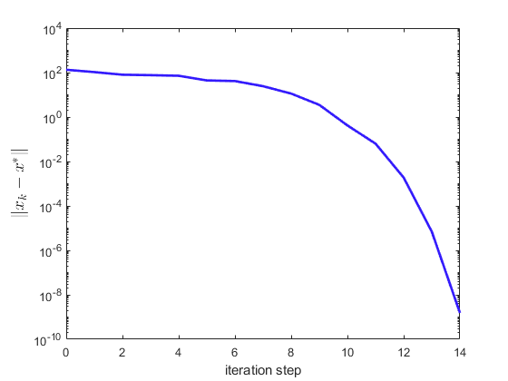
(a) rcv1

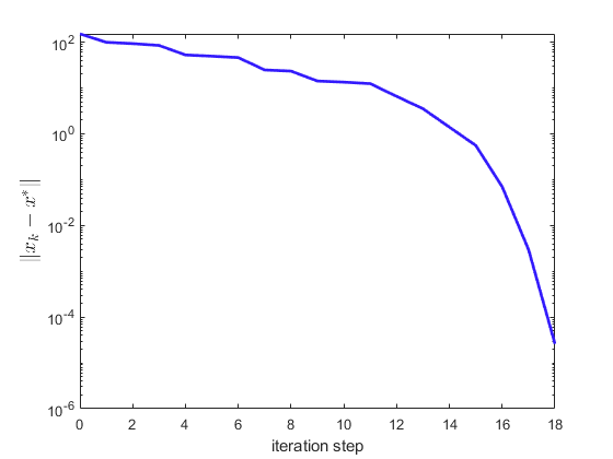
(b) news20

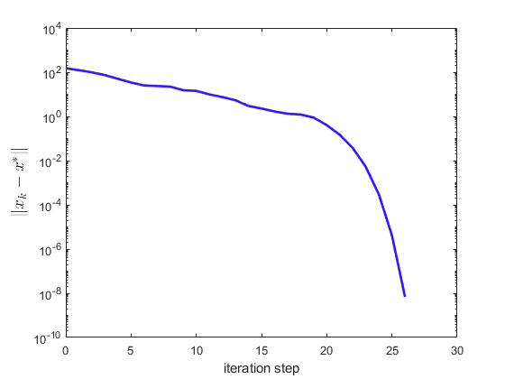
(c) real-sim

Figure 1: Convergence behavior of the sequence of $\{\|x_{k}-x^{*}\|\}_{k\geq 0}$

5.2 Numerical results on LASSO problem

We consider the $\ell_{1}$-norm regularized least squares problem:

$$\min_{x\in\mathbb{R}^{n}}\frac{1}{2}\|Ax-b\|_{2}^{2}+\gamma\|x\|_{1}.$$

Here, $A\in\mathbb{R}^{m\times n}$ and $b\in\mathbb{R}^{m}$ are given data samples; $\gamma$ is a given regularization parameter. Closely related to the LASSO problem is the Basis Pursuit problem, which is a convex optimization problem that seeks the sparsest solution to an underdetermined linear system of equations. The Basis Pursuit (BP) problem can be formulated as

$$\min_{x\in\mathbb{R}^{n}}\|x\|_{1}\quad\text{ s.t. }\quad Ax=b.$$

The theory for penalty functions implies that the solution of the LASSO problem goes to the solution of BP problem as $\gamma$ goes to zero.

In our experiment, we compare our algorithm with other state-of-the-art algorithms on large-scale reconstruction problems. The test problems are from [28, 17], which are generated by the following procedure. Firstly, we randomly generate a sparse solution $\bar{x}\in\mathbb{R}^{n}$ with $k$ nonzero entries, where $n=512^{2}=262144$ and $k=\left\lfloor n/40\right\rfloor=6553$. The $k$ different indices are uniformly chosen from $\{1,2,\ldots,n\}$ and we set the magnitude of each nonzero element by $\bar{x}_{i}=\eta_{1}(i)10^{d\eta_{2}(i)/20}$, where $\eta_{1}(i)$ is randomly chosen from $\{-1,1\}$ with probability $\frac{1}{2}$, respectively, $\eta_{2}(i)$ is uniformly distributed in $[0,1]$ and $d$ is a dynamic range which can influence the efficiency of the solvers. Then we choose $m=n/8=32768$ random cosine measurements, i.e., $Ax=(dct(x))_{J}$, where $J$ contains $m$ different indices randomly chosen from $\{1,2,\ldots,n\}$ and $dct$ is the discrete cosine transform. Finally, the input data is specified by $b=A\bar{x}+\epsilon$, where components of $\epsilon$ are i.i.d Gaussian noises with a standard deviation $\bar{\sigma}=0.1$.

We recognize that the performance of most of the existing second-order and fast first-order algorithms for large-scale reconstruction problems has been studied in [28], suggesting that ASSN, ASLB [28] have outperformed the other solvers like SNF [17], FPC_AS [22] and SpaRSA [25]. Therefore, we compare our algorithm with ASSN, ASLB on the LASSO problem and the results are presented in Table 5.

The parameters of our algorithm align with those specified in ASSN. We conducted experiments across 10 independent runs for varying dynamic ranges. To ensure fair comparison, we adopted the same stopping criterion as [28], terminating the algorithm when the tolerance reached $10^{-6}$. Since matrix-vector operations ($A$ and $A^{T}$) dominate computational overhead, we primarily use the total number of $A$ and $A^{T}$ calls ($N_{A}$) to evaluate solver efficiency. Detailed results are presented in Table 5.

The performance of our algorithm is competitive with that of ASSN, indicating that our method is also efficient for solving large-scale reconstruction problems. The results from ASLB are slightly better than those of ASSN and our algorithm, which is expected as using the LBFGS method to solve the Newton equation may perform better than the CG method.

Table 5: Computational results on LASSO problem: $N_{A}$ denotes the total number of calls to $A$ and $A^{T}$ and the CPU time (in seconds) is averaged over 10 independent runs.

Dynamic range		ASSN	ASLB(1)	ASLB(2)	TMAP
20dB	$N_{A}$	298.2	275.6	269.0	300.6
	time	1.31	1.54	1.47	1.30
40dB	$N_{A}$	459.2	321.0	329.8	408.9
	time	2.51	2.19	2.25	2.32
60dB	$N_{A}$	635.4	358.6	384.0	624.9
	time	2.29	1.65	1.77	2.23
80dB	$N_{A}$	858.2	402.6	438.6	791.5
	time	2.99	1.75	1.89	2.74

6 Discussion

In this section, we discuss the comparison between the two-metric projection method and our algorithm for solving Eq. 1.

Bound-constrained formulation of $\ell_{1}$-norm minimization

Let $x=x^{+}-x^{-}$ in Eq. 1, where $x^{+}=\max(0,x)$ and $x^{-}=-\min(0,x)$. Then Eq. 1 can be reformulated as the following constrained problem

(32) $$\begin{array}[]{rl}\min\limits_{x^{+},x^{-}\in\mathbb{R}^{n}}&f\left(x^{+}-x^{-}\right)+\gamma\sum_{i}\left[x_{i}^{+}+x_{i}^{-}\right]\\ \text{ s.t. }&x^{+}\geq 0,\quad x^{-}\geq 0.\end{array}$$

This is a bound-constrained problem with $2n$ variables. We may directly apply two-metric projection to this formulation.

Connection to our algorithm

We write the index set in two-metric projection method for Eq. 32 specifically. Suppose that at $k$th iteration, $I_{k}^{1}$ and $I_{k}^{2}$ are the “$I_{k}^{-}$ part” corresponding to $x_{k}^{+}$ and $x_{k}^{-}$ respectively. Let $x_{k}\triangleq x_{k}^{+}-x_{k}^{-}$. Given an $\epsilon_{k}$, we have

$$I_{k}^{1} =\{i\mid 0\leq(x_{k}^{+})^{i}\leq\epsilon_{k},g_{k}^{i}+\gamma\leq 0\}\cup\{i\mid(x_{k}^{+})^{i}>\epsilon_{k}\},$$

$$I_{k}^{2} =\{i\mid 0\leq(x_{k}^{-})^{i}\leq\epsilon_{k},-g_{k}^{i}+\gamma\leq 0\}\cup\{i\mid(x_{k}^{-})^{i}>\epsilon_{k}\}.$$

Compare $I_{k}^{1}$ and $I_{k}^{2}$ with $I_{k}^{-+}$ and $I_{k}^{--}$ corresponding to $x_{k}$ in our algorithm. If $x_{k}^{+}=\max(0,x_{k})$ and $x_{k}^{-}=-\min(0,x_{k})$ and $\epsilon_{k}$ is the same, then we have

$$I_{k}^{-+}\subseteq I_{k}^{1},\quad I_{k}^{--}\subseteq I_{k}^{2}.$$

It is worth noting that we always have $I_{k}^{-+}\cap I_{k}^{--}=\emptyset$ in our algorithm, but $I_{k}^{1}\cap I_{k}^{2}\neq\emptyset$ may happen.

Potential issue

Unfortunately, it will lead to numerical instability if we directly apply the two-metric projection method to Eq. 32. To illustrate this, we consider the eigendecomposition of Hessian.

$$\nabla^{2}f(x_{k})=Q^{T}\Lambda Q$$

Let $Q=[q_{1},q_{2},\ldots,q_{n}]$, and $Q_{1}=[q_{i_{1}}]_{i_{1}\in I_{k}^{1}}$, $Q_{2}=[q_{i_{2}}]_{i_{2}\in I_{k}^{2}}$. Then, in two-metric projection, we need to solve a Newton equation as follows,

$$\begin{bmatrix}Q_{1}^{T}\Lambda Q_{1}&-Q_{1}^{T}\Lambda Q_{2}\\ -Q_{2}^{T}\Lambda Q_{1}&Q_{2}^{T}\Lambda Q_{2}\end{bmatrix}\begin{bmatrix}p_{1}\\ p_{2}\end{bmatrix}=\begin{bmatrix}\nabla f_{I_{k}^{1}}(x_{k})+\gamma{\mathbf{1}}_{I_{k}^{1}}\\ -\nabla f_{I_{k}^{2}}(x_{k})+\gamma{\mathbf{1}}_{I_{k}^{2}}\end{bmatrix},$$

where ${\mathbf{1}}$ denotes the vector of all $1$ of appropriate dimension. This is equivalent to

$$\begin{bmatrix}Q_{1}&Q_{2}\end{bmatrix}^{T}\Lambda\begin{bmatrix}Q_{1}&Q_{2}\end{bmatrix}\begin{bmatrix}p_{1}\\ -p_{2}\end{bmatrix}=\begin{bmatrix}\nabla f_{I_{k}^{1}}(x_{k})+\gamma{\mathbf{1}}_{I_{k}^{1}}\\ \nabla f_{I_{k}^{2}}(x_{k})-\gamma{\mathbf{1}}_{I_{k}^{2}}\end{bmatrix}.$$

If $I_{k}^{1}\cap I_{k}^{2}\neq\emptyset$, then $Q_{1}$ and $Q_{2}$ have at least one identical column, and Newton’s equation is unsolvable. This could happen in practice especially for large-scale problems, and even when $\nabla^{2}f(x_{k})\succ 0$. Schmidt also pointed out this issue in their paper [19].

This defect in the algorithm design may be intrinsic. Note that we may add regularization to the singular Hessian for salvage. However, since the original Newton system may not have a solution, this approach may be faced with numerical instability when the regularization parameter tends to $0$. In general, the more accurate is the Hessian approximation, the less stable is the solution.

Another salvage is using (limited) BFGS to approximate Hessian. Schmidt proposed ProjectionL1 for problem (32) in [20], and this is a variant of the two-metric projection method that we discuss in this section. They used two Quasi-Newton methods to approximate Hessian: BFGS and L-BFGS. L-BFGS is more suitable to large-scale problems.

We conduct numerical experiments to compare our TMAP and ProjectionL1-LBFGS. Let the algorithms terminate with a highly accurate solution when the iterate $x_{k}$ satisfies

$$r(x_{k})=\|x_{k}-\operatorname{prox}_{h}(x_{k}-\nabla f(x_{k}))\|\leq 10^{-8}$$

or $k=200$. The result in Table 6 shows that ProjectionL1-LBFGS does not perform as good as TMAP, especially in the large-scale scenario.

Table 6: Computational results between TMAP and ProjectionL1-LBFGS

dataset	algorithm	iter.	time
rcv1	TMAP	12	0.200
	ProjectionL1-LBFGS	105	0.991
news20	TMAP	17	1.931
	ProjectionL1-LBFGS	200	236.228
real-sim	TMAP	20	1.503
	ProjectionL1-LBFGS	200	4.450

7 Conclusion

In this paper, we propose a two-metric adaptive projection method for solving the $\ell_{1}$-norm minimization problem. Compared with the two-metric projection method proposed by Bertsekas and ProjectionL1 proposed by Schmidt to solve the equivalent bound-constrained problem, our algorithm does not require an exact solver of Newton system or the strong convexity of $f$. Moreover, it can be shown to converge globally to an optimal solution and have local superlinear convergence rate. The key to our analysis is the Error Bound condition, which is a weaker condition than the strong convexity of $f$ and sufficient second-order condition for problem Eq. 1. We also provide a complexity guarantee for our algorithm in the nonconvex setting.

We compared our algorithm with other competitive methods on the $\ell_{1}$-regularized logistic regression problem and LASSO problem. The numerical results show that our algorithm can identify the active manifold effectively and achieve the desired accuracy with fewer iterations and less computational time than other methods on logistic regression problems. On the LASSO problem, our algorithm is competitive with ASSN and ASLB, which are a type of semi-smooth Newton method and its LBFGS variant for large-scale reconstruction problems respectively.

There are several future directions worth studying on the two-metric adaptive projection method. First, we can extend our algorithm to solve other separable regularized optimization problems, such as the $\ell_{0}$-regularized problem. Second, we can use LBFGS to approximate the Hessian matrix in our algorithm to improve the computational efficiency.

References

- [1] P.-A. Absil, R. Mahony, and R. Sepulchre, Optimization algorithms on matrix manifolds, Princeton University Press, 2008.
- [2] H. Attouch, J. Bolte, P. Redont, and A. Soubeyran, Proximal alternating minimization and projection methods for nonconvex problems: An approach based on the kurdyka-łojasiewicz inequality, Mathematics of operations research, 35 (2010), pp. 438–457.
- [3] G. Bareilles, F. Iutzeler, and J. Malick, Newton acceleration on manifolds identified by proximal gradient methods, Mathematical Programming, 200 (2023), pp. 37–70.
- [4] H. H. Bauschke, P. L. Combettes, H. H. Bauschke, and P. L. Combettes, Correction to: convex analysis and monotone operator theory in Hilbert spaces, Springer, 2017.
- [5] A. Beck, First-order methods in optimization, SIAM, 2017.
- [6] A. Beck and M. Teboulle, A fast iterative shrinkage-thresholding algorithm for linear inverse problems, SIAM journal on imaging sciences, 2 (2009), pp. 183–202.
- [7] D. P. Bertsekas, Projected newton methods for optimization problems with simple constraints, SIAM Journal on control and Optimization, 20 (1982), pp. 221–246.
- [8] N. Boumal, An introduction to optimization on smooth manifolds, Cambridge University Press, 2023, https://doi.org/10.1017/9781009166164, https://www.nicolasboumal.net/book.
- [9] S. Boyd, N. Parikh, E. Chu, B. Peleato, J. Eckstein, et al., Distributed optimization and statistical learning via the alternating direction method of multipliers, Foundations and Trends® in Machine learning, 3 (2011), pp. 1–122.
- [10] Y. Carmon, J. C. Duchi, O. Hinder, and A. Sidford, Lower bounds for finding stationary points i, Mathematical Programming, 184 (2020), pp. 71–120.
- [11] C.-C. Chang, Libsvm data: Classification, regression, and multi-label, http://www. csie. ntu. edu. tw/˜ cjlin/libsvmtools/datasets/, (2008).
- [12] E. M. Gafni and D. P. Bertsekas, Two-metric projection methods for constrained optimization, SIAM Journal on Control and Optimization, 22 (1984), pp. 936–964.
- [13] W. L. Hare and A. S. Lewis, Identifying active constraints via partial smoothness and prox-regularity, Journal of Convex Analysis, 11 (2004), pp. 251–266.
- [14] J. Hu, T. Tian, S. Pan, and Z. Wen, On the local convergence of the semismooth newton method for composite optimization, arXiv preprint arXiv:2211.01127, (2022).
- [15] C.-p. Lee, Accelerating inexact successive quadratic approximation for regularized optimization through manifold identification, Mathematical Programming, 201 (2023), pp. 599–633.
- [16] A. S. Lewis and J. Liang, Partial smoothness and constant rank, arXiv preprint arXiv:1807.03134, (2018).
- [17] A. Milzarek and M. Ulbrich, A semismooth newton method with multidimensional filter globalization for l_1-optimization, SIAM Journal on Optimization, 24 (2014), pp. 298–333.
- [18] Y. Nesterov, Gradient methods for minimizing composite functions, Mathematical programming, 140 (2013), pp. 125–161.
- [19] M. Schmidt, Graphical model structure learning with l1-regularization, University of British Columbia, (2010), p. 26.
- [20] M. Schmidt, G. Fung, and R. Rosales, Fast optimization methods for l1 regularization: A comparative study and two new approaches, in Machine Learning: ECML 2007: 18th European Conference on Machine Learning, Warsaw, Poland, September 17-21, 2007. Proceedings 18, Springer, 2007, pp. 286–297.
- [21] P. Tseng and S. Yun, A coordinate gradient descent method for nonsmooth separable minimization, Mathematical Programming, 117 (2009), pp. 387–423.
- [22] Z. Wen, W. Yin, D. Goldfarb, and Y. Zhang, A fast algorithm for sparse reconstruction based on shrinkage, subspace optimization, and continuation, SIAM Journal on Scientific Computing, 32 (2010), pp. 1832–1857.
- [23] S. J. Wright, Identifiable surfaces in constrained optimization, SIAM Journal on Control and Optimization, 31 (1993), pp. 1063–1079.
- [24] S. J. Wright, Coordinate descent algorithms, Mathematical programming, 151 (2015), pp. 3–34.
- [25] S. J. Wright, R. D. Nowak, and M. A. Figueiredo, Sparse reconstruction by separable approximation, IEEE Transactions on signal processing, 57 (2009), pp. 2479–2493.
- [26] S. J. Wright and B. Recht, Optimization for data analysis, Cambridge University Press, 2022.
- [27] H. Wu and Y. Xie, A study on two-metric projection methods, arXiv preprint arXiv:2409.05321, (2024).
- [28] X. Xiao, Y. Li, Z. Wen, and L. Zhang, A regularized semi-smooth newton method with projection steps for composite convex programs, Journal of Scientific Computing, 76 (2018), pp. 364–389.
- [29] G.-X. Yuan, C.-H. Ho, and C.-J. Lin, An improved glmnet for l1-regularized logistic regression, The Journal of Machine Learning Research, 13 (2012), pp. 1999–2030.
- [30] M.-C. Yue, Z. Zhou, and A. M.-C. So, A family of inexact sqa methods for non-smooth convex minimization with provable convergence guarantees based on the luo–tseng error bound property, Mathematical Programming, 174 (2019), pp. 327–358.
- [31] S. Yun and K.-C. Toh, A coordinate gradient descent method for l1-regularized convex minimization, Computational Optimization and Applications, 48 (2011), pp. 273–307.
- [32] Z. Zhou and A. M.-C. So, A unified approach to error bounds for structured convex optimization problems, Mathematical Programming, 165 (2017), pp. 689–728.