Rotating Topological Stars

Abstract

We construct a three-parameter family of smooth and horizonless rotating solutions of Einstein-Maxwell theory with Chern-Simons term in five dimensions and discuss their stringy origin in terms of three-charge brane systems in Type IIB and M-theory. The general solution interpolates smoothly between Kerr and static Topological Star geometries. We show that for specific choices of the parameters and quantized values of the angular momentum the geometry terminates on a smooth five-dimensional cap, and it displays neither ergoregion nor closed timelike curves and a region of Gregory-Laflamme stability. We discuss the dimensional reduction to four dimensions and the propagation of particles and waves showing that geodetic motion is integrable and the radial and angular propagation of scalar perturbations can be separated and described in terms of two ordinary differential equations of confluent Heun type.

1 Introduction

Deciphering the intime structure of black holes (BHs) is one of the most fascinating and active endeavours in the quest for a quantum theory of gravity. One of the most credited proposals Mathur:2005zp , motivated by String Theory, posits the absence of both the horizon and the curvature singularity. In this framework, BHs are viewed as statistical ensembles involving a huge number of smooth and horizonless micro-state geometries, known as fuzzballs. Given the existence of no-go theorems in four dimensions Einstein:1943ixi , fuzzball geometries are typically built as solutions of five or higher-dimensional gravity theories, blowing up near the would-be horizon, see Giusto:2004id ; Giusto:2004ip ; Bena:2005va ; Bena:2007kg ; Bena:2015bea ; Bah:2021jno for a few examples within this class.

A particularly simple class of solutions, that may be viewed as a “caricature” of spherically-symmetric fuzzballs, are known as Topological Stars Bah:2020ogh ; Bah:2020pdz ; Bah:2022yji ; Chakraborty:2025ger (Top Stars or TS for brevity). TS are static, smooth and horizonless solutions of five-dimensional Einstein-Maxwell theory supported by fluxes. Several dynamical properties of these solutions have been studied in the recent literature Heidmann:2022ehn ; Bianchi:2023sfs ; Heidmann:2023ojf ; Bena:2024hoh ; Melis:2024kfr ; Dima:2025zot ; Bianchi:2024vmi ; Bianchi:2024rod ; DiRusso:2025lip , including their linear stability, deformability, echoes due to late-time emission of (scalar) waves (as a proxy for gravitational waves) and radiation losses in the Self-Force approach, both for bound and unbound orbits.

Given the wealth of data that the LIGO-Virgo-KAGRA collaboration is collecting, and the one expected from the next generation of both ground-based and space-based experiments, one may envisage the possibility in the near future of being able to discriminate black holes from fuzzballs or other Exotic Compact Objects (ECO) from their gravitational-wave signals Bianchi:2020bxa ; Bena:2020see ; Bianchi:2020miz ; Bena:2020uup ; Ikeda:2021uvc ; Bah:2021jno ; Staelens:2023jgr . For this reason it is urgent to find smooth horizonless counterparts of Kerr BHs in the simple-minded (‘caricature’) version of the fuzzball proposal for compact rotating objects.

The aim of the present investigation is to built a class of smooth horizonless solutions of minimal supergravity in five dimensions carrying non-trivial angular momentum in four-dimensions after reduction on a compact circle. A three parameter family of solutions of this theory parametrized by a mass, a rotation parameter $a$ and a duality phase was found in Compere:2009zh . Here we consider solutions obtained from this family by analytic continuation to the imaginary branch where $a^{2}<0$. The resulting solution, parametrized by three real numbers, $r_{s}$, $r_{b}$ and $a^{2}$ interpolate between the static TS solution at $a\to 0$, and the Kerr BH at $r_{b}\to 0$. We find that for specific choices of the parameters the BH curvature singularity can be hidden inside of a cap where space terminates. Moreover, for quantized choices of the angular momentum parameter, in the branch where $a^{2}<0$, the resulting geometry is horizonless and smooth everywhere. We will refer to these solution as a “Rotating Topological Star” (RTS for brevity).

We will study the properties of RTS, their reduction to four dimensions, and their embedding in String theory as ‘harmonic superpositions’ of three stacks of M5-branes in M-theory or, as bound-states of KK-monopoles and D1-branes and D5-branes in Type IIB superstring theory. We will also briefly discuss the propagation of scalar and gravitational waves in the RTS geometry. In particular we show that, like in the Kerr case, the scalar wave equation can be separated into two ordinary differential equations of confluent Heun type.

The plan of the paper is the following. In section 2, we discuss the M- and String origin of static Top(ological) Stars (TS). In section 3, we introduce the RTS solutions and determine the conditions under which the geometry is horizonless and smooth. We also show that no ergoregion is present in the RTS regime. In section 4, we discuss the reduction to four dimensions and compute mass, charges and angular momentum that turn out to be incompatible with the BH regime. In section 5 we discuss geodetic motion, show that it’s integrable and identify the light-rings in the equatorial plane. Finally in Section 6 we study scalar wave perturbations and show that both the angular and radial dynamics are governed by Confluent Heun Equations (CHE’s) that can be related to quantum Seiberg-Witten curves for ${\cal N}=2$ super Yang Mills (SYM) theories with three fundamental hyper-multiplets. We also discuss the extremal limit $r_{b}=r_{s}$.

2 M- and String origin of static Topological Stars

Let us consider the Einstein-Maxwell action in five dimensions,

$$S\,=\,\frac{1}{2\kappa_{5}^{2}}\int\mathrm{d}^{5}x\sqrt{-g}\left(R-\frac{1}{4}|F_{(2)}|^{2}\right)\,,$$ (2.1)

where $\kappa_{5}^{2}=8\pi G_{5}$ denotes the five-dimensional gravitational coupling constant and $F_{(2)}\,=\,\mathrm{d}A_{(1)}$. A solution of this theory, found by Horowitz and Strominger in Horowitz:1991cd , is the following:

$$\mathrm{d}s^{2}\,= -f_{s}(r)\mathrm{d}t^{2}+\frac{\mathrm{d}r^{2}}{f_{s}(r)f_{b}(r)}+r^{2}\left(\mathrm{d}\theta^{2}+\sin^{2}\theta\mathrm{d}\phi^{2}\right)+f_{b}(r)\mathrm{d}y^{2}\ ,$$ (2.2)

$$A_{(1)}\,= P\,\cos\theta\,\mathrm{d}\phi\ ,$$

where

$$f_{s}(r)\,=\,\left(1-\frac{r_{s}}{r}\right)\,,\hskip 28.45274ptf_{b}(r)\,=\,\left(1-\frac{r_{b}}{r}\right)\,,$$ (2.3)

and

$$P^{2}\,=\,3\,r_{s}r_{b}\,.$$ (2.4)

In the regime $r_{s}\geq r_{b}$, which was the one originally studied in Horowitz:1991cd , the solution describes a magnetically-charged black string. The limiting case $r_{s}=r_{b}$ represents an extremal black string, which displays an AdS${}_{3}\times S^{2}$ near-horizon geometry. The analysis of the solution in the regime $r_{b}>r_{s}$ has been recently addressed by Bah and Heidmann in Bah:2020ogh , where it has been shown to correspond to a smooth horizonless soliton, called ‘Topological Star’ or Top Star (TS) for brevity.

There exists also an electric version of the Topological Star, where the metric (2.2) is instead supported by the electric two-form charge

$$B_{(2)}\,= \frac{Q}{r}\,\mathrm{d}t\wedge\mathrm{d}y\ ,$$ (2.5)

solving the Einstein equation describing gravity minimally coupled to the three-form field strength $H_{(3)}=dB_{2}$

$$S_{5}\,=\,\frac{1}{2\kappa_{5}^{2}}\int\mathrm{d}^{5}x\sqrt{-g}\left(R-\frac{1}{12}|H_{(3)}|^{2}\right)\,,$$ (2.6)

The solution we have just presented can be obtained from three-charge configurations consisting of non-extremal brane systems in string or M-theory, upon a suitable identification of the charges. These can be viewed as dyonic solutions of minimal supergravity, obtained by identifying the three U(1) gauge fields of the STU supergravity model in five dimensions Sierra:1985ax , thus extending in the bosonic sector Einstein-Maxwell (EM) with a Chern-Simons (CS) term. Denoting by $Q_{i}$ and $P_{i}$, the corresponding electric and magnetic charges with respect to the three U(1) gauge fields of the STU model, Einstein equations require

$$\sum_{i=1}^{3}(P_{i}^{2}+Q_{i}^{2})=\,3r_{s}r_{b}\,.$$ (2.7)

We start by reviewing the non-extremal deformations of BPS M-branes, and then we discuss in turn the embedding of electric and magnetic TS in string/M-theory.

2.1 Non-BPS deformations of M-branes

In this section we review two different non-extremal deformations of BPS M-branes. An analogous story applies, mutatis mutandis, to D-branes in string theory as well. We start by considering a BPS M5-brane described by the following eleven-dimensional supergravity solution Gueven:1992hh ; Ortin:2015hya ,

$$\begin{array}[]{lcl}\mathrm{d}s_{11}^{2}&=&H^{-1/3}\mathrm{d}s_{\mathbb{R}^{1,5}}^{2}+H^{2/3}\left(\mathrm{d}r^{2}+r^{2}\mathrm{d}s_{S^{4}}^{2}\right)\ ,\\[5.69054pt] A_{(6)}&=&(H^{-1}-1)\,\mathrm{vol}_{\mathbb{R}^{1,5}}\ ,\end{array}$$ (2.8)

where $H$ is a harmonic function on the transverse $\mathbb{R}^{5}$ and $\mathrm{d}s_{S^{4}}^{2}$ is the metric of a unit $S^{4}$. Demanding spherical symmetry,

$$H=1+\frac{Q_{5}}{r^{3}}\,.$$ (2.9)

The first way to make the above M5 become non-extremal is to add a blackening factor,

$$W_{1}=1-\frac{\omega_{1}}{r^{3}}\,,$$ (2.10)

with $\omega_{1}>0$ through

$$\begin{array}[]{lcl}\mathrm{d}s_{11}^{2}&=&H^{-1/3}\left(-W_{1}\,\mathrm{d}t^{2}+\mathrm{d}s_{\mathbb{R}^{5}}^{2}\right)+H^{2/3}\left(\frac{\mathrm{d}r^{2}}{W_{1}}+r^{2}\mathrm{d}s_{S^{4}}^{2}\right)\ ,\\[5.69054pt] A_{(6)}&=&\gamma_{1}\,(H^{-1}-1)\,\mathrm{vol}_{\mathbb{R}^{1,5}}\ ,\end{array}$$ (2.11)

with $\gamma_{1}=\sqrt{1+\frac{\omega_{1}}{Q_{5}}}$ the off-extremality parameter. A second way of going non-extremal is to add a cap-off factor,

$$W_{2}\,=\,1-\frac{\omega_{2}}{r^{3}}\,,$$ (2.12)

still with $\omega_{2}>0$. The solution is modified as follows

$$\begin{array}[]{lcl}\mathrm{d}s_{11}^{2}&=&H^{-1/3}\left(W_{2}\,\mathrm{d}y^{2}+\mathrm{d}s_{\mathbb{R}^{1,4}}^{2}\right)+H^{2/3}\left(\frac{\mathrm{d}r^{2}}{W_{2}}+r^{2}\mathrm{d}s_{S^{4}}^{2}\right)\ ,\\[5.69054pt] A_{(6)}&=&\gamma_{2}\,(H^{-1}-1)\,\mathrm{vol}_{\mathbb{R}^{1,5}}\ ,\end{array}$$ (2.13)

where $\gamma_{2}=\sqrt{1+\frac{\omega_{2}}{Q_{5}}}$ the off-extremality parameter. Note that in this case space terminates at $r=\omega_{2}^{1/3}$, provided that the $y$ coordinate be compact. It is worth noticing that, both non-extremal M5-branes are obtained by replacing the eleven-dimensional flat space where the M5 branes live in with (Euclidean) Schwarzschild-Tangherlini (ST) Ricci-flat geometries: $\textrm{ST}_{1,5}\times\mathbb{R}^{5}$, for the former, or ${\mathbb{R}^{1,4}}\times\textrm{EST}_{6}$, for the latter. We will show that both of these non-extremal deformations may be performed simultaneously in three-charge brane systems, just at the price of slightly modifying the ansatz for the flux.

2.2 M-theory embedding of a magnetic Topological Stars

Let us consider the intersection of three mutually orthogonal M5-branes as shown in table 1.

branes	$t$	$y$	$x^{1}$	$x^{2}$	$x^{3}$	$x^{4}$	$x^{5}$	$x^{6}$	$r$	$\theta$	$\phi$
M51	$-$	$-$	$\cdot$	$\cdot$	$-$	$-$	$-$	$-$	$\cdot$	$\cdot$	$\cdot$
M52	$-$	$-$	$-$	$-$	$\cdot$	$\cdot$	$-$	$-$	$\cdot$	$\cdot$	$\cdot$
M53	$\underbrace{-}_{W_{1}}$	$\underbrace{-}_{W_{2}}$	$-$	$-$	$-$	$-$	$\cdot$	$\cdot$	${\cdot}$	$\cdot$	$\cdot$

Table 1: (Non-)extremal intersection of three orthogonal M5-branes.

The corresponding 11d supergravity solution reads

$$\hskip-19.91692pt\begin{array}[]{lcl}\mathrm{d}s_{11}^{2}&=&H_{1}^{-1/3}H_{2}^{-1/3}H_{3}^{-1/3}\left(-W_{1}\,\mathrm{d}t^{2}+W_{2}\,\mathrm{d}y^{2}\right)+H_{1}^{2/3}H_{2}^{2/3}H_{3}^{2/3}\left(\dfrac{\mathrm{d}r^{2}}{W_{1}W_{2}}+r^{2}\mathrm{d}s_{S^{2}}^{2}\right)\\[5.69054pt] &&+H_{1}^{-1/3}H_{2}^{-1/3}H_{3}^{-1/3}\left(H_{2}\,\mathrm{d}s_{\mathbb{T}_{1}^{2}}^{2}+H_{3}\,\mathrm{d}s_{\mathbb{T}_{2}^{2}}^{2}+H_{1}\,\mathrm{d}s_{\mathbb{T}_{3}^{2}}^{2}\right)\ ,\\[5.69054pt] F_{(4)}&=&\left(\gamma_{1}\,Q_{1}\mathrm{vol}_{\mathbb{T}_{1}^{2}}+\gamma_{2}\,Q_{2}\mathrm{vol}_{\mathbb{T}_{2}^{2}}+\gamma_{3}\,Q_{3}\mathrm{vol}_{\mathbb{T}_{3}^{2}}\right)\wedge\mathrm{vol}_{S^{2}}\ ,\end{array}$$ (2.14)

where

$$H_{i}\,=\,1+\frac{Q_{i}}{r}\ ,\ i=1,2,3\ ,\quad\quad W_{a}\,=\,1-\frac{\omega_{a}}{r}\ ,\ a=1,2\ ,$$ (2.15)

with $\ \gamma_{i}\,=\,\sqrt{\left(1+\dfrac{\omega_{1}}{Q_{i}}\right)\left(1+\dfrac{\omega_{2}}{Q_{i}}\right)}\$.

When $W_{1}=W_{2}=1$, the system is ${1}/{8}$ – BPS, with near-horizon geometry $\textrm{AdS}_{3}\times S^{2}$ preserving eight real supercharges.

To obtain the TS, we identify $Q_{1}=Q_{2}=Q_{3}\equiv\widehat{Q}$, leading to

$$\mathrm{d}s_{11}^{2}\,=\,H^{-1}\left(-W_{1}\,\mathrm{d}t^{2}+W_{2}\,\mathrm{d}y^{2}\right)+H^{2}\left(\frac{\mathrm{d}r^{2}}{W_{1}W_{2}}+r^{2}\mathrm{d}s_{S^{2}}^{2}\right)+\mathrm{d}s_{\mathbb{T}^{6}}^{2}\ ,$$ (2.16)

with $H=1+\frac{\widehat{Q}}{r}=H_{1}=H_{2}=H_{3}$. The metric in (2.16) is the direct product of the TS metric (2.2) and a six-torus, upon identifying $r_{s}\,=\,\widehat{Q}+\omega_{1}$, $r_{b}\,=\,\widehat{Q}+\omega_{2}$, and sending $r\to r-\widehat{Q}$, that we will henceforth continue to denote by $r$. The metric is supported by the magnetic charge $P^{2}=3r_{s}r_{b}$. We stress that thanks to the identification of the charges $Q_{a}$ and thus of the harmonic functions $H_{a}$ the six-torus completely factorizes from the rest and has fixed volume/radii.

2.3 IIB embedding of a dyonic Topological Stars

The type IIB brane picture of a dyonic TS may be obtained from the previous M5 intersection by a chain of dualities. In particular, we first reduce on $S^{1}_{x^{6}}$ to obtain an NS5 – D4 – D4 intersection in type IIA. Subsequently, we perform three T-dualities along $x^{3,4,5}$ to get the IIB setup depicted in table 2.

branes	$t$	$y$	$x^{1}$	$x^{2}$	$x^{3}$	$x^{4}$	$x^{5}$	$r$	$\theta$	$\phi$
KK5${}_{\textrm{B}}$	$-$	$-$	$-$	$-$	$-$	$-$	iso	${\cdot}$	$\cdot$	$\cdot$
D1	$-$	$-$	$\cdot$	$\cdot$	$\cdot$	$\cdot$	$\cdot$	$\cdot$	$\cdot$	$\cdot$
D5	$\underbrace{-}_{W_{1}}$	$\underbrace{-}_{W_{2}}$	$-$	$-$	$-$	$-$	$\cdot$	$\cdot$	$\cdot$	$\cdot$

Table 2: (Non-)extremal KK5 – D1 – D5 intersection.

The corresponding IIB supergravity (string frame) solution reads

$$\hskip-19.91692pt\begin{array}[]{lcl}\mathrm{d}s_{10}^{2}&=&H_{1}^{-1/2}H_{2}^{-1/2}\left(-W_{1}\,\mathrm{d}t^{2}+W_{2}\,\mathrm{d}y^{2}\right)+H_{1}^{1/2}H_{2}^{1/2}H_{3}\left(\dfrac{\mathrm{d}r^{2}}{W_{1}W_{2}}+r^{2}\mathrm{d}s_{S^{2}}^{2}\right)\\[8.53581pt] &&+H_{1}^{1/2}H_{2}^{1/2}H_{3}^{-1}\left(dx^{5}+\gamma_{3}\,Q_{3}\cos\theta\,\mathrm{d}\phi\right)^{2}+H_{1}^{1/2}H_{2}^{-1/2}\mathrm{d}s_{\mathbb{T}^{4}}\ ,\\[5.69054pt] e^{\Phi}&=&H_{1}^{1/2}H_{2}^{-1/2}\ ,\\[5.69054pt] C_{(2)}&=&\gamma_{1}\,\left(H_{1}^{-1}-1\right)\mathrm{d}t\wedge\mathrm{d}y\ ,\\[5.69054pt] C_{(6)}&=&\gamma_{2}\,\left(H_{2}^{-1}-1\right)\mathrm{d}t\wedge\mathrm{d}y\wedge\mathrm{vol}_{\mathbb{T}^{4}}\ ,\end{array}$$ (2.17)

where

$$H_{i}\,=\,1+\frac{Q_{i}}{r}\ ,\ i=1,2,3\ ,\quad\quad W_{a}\,=\,1-\frac{\omega_{a}}{r}\ ,\ a=1,2\ ,$$ (2.18)

with $\ \gamma_{i}\,=\,\sqrt{\left(1+\dfrac{\omega_{1}}{Q_{i}}\right)\left(1+\dfrac{\omega_{2}}{Q_{i}}\right)}\$.

The D1-branes are smeared along the directions $x^{1,2,3,4,5}$, while the D5-branes are smeared along the direction $x^{5}$, the isometric direction for the KK monopole. When $W_{1}=W_{2}=1$, the system is ${1}/{8}$ – BPS with near-horizon geometry $\textrm{AdS}_{3}\times S^{2}$ preserving eight real supercharges.

The TS metric (2.2) is obtained again identifying the three charges $Q_{1}=Q_{2}=Q_{3}\equiv\widehat{Q}$, dimensionally reducing along the ${\mathbb{T}^{4}}$ and $x^{5}$-directions, setting $r_{s}=\widehat{Q}+\omega_{1}$, $r_{b}=\widehat{Q}+\omega_{2}$, and sending $r\to r-\widehat{Q}$. The metric is now supported by a magnetic charge $P^{2}=r_{s}r_{b}$ coming from the KK gauge field with charge $\gamma_{3}Q_{3}$ and the two two-forms descending from the RR $C_{(2)}$ and $C_{(6)}$ potentials carrying a total electric charge $Q^{2}=2r_{s}r_{b}$. As before, thanks to the identification of the charges $Q_{a}$ and thus of the harmonic functions $H_{a}$ the four-torus completely factorizes from the rest and has fixed volume/radii, while the $x^{5}$ circle with constant radius is fibered over the five-dimensional TS base space due the KK monopole.

3 Rotating Topological Stars

The goal of this section is to study solutions of minimal supergravity in five dimensions describing rotating topological solitons, to which we refer as Rotating Topological Stars (or RTS for brevity). Our conventions are such that the bosonic action of minimal supergravity Gunaydin:1983bi is given by

$$S\,=\,\frac{1}{2\kappa_{5}^{2}}\int\mathrm{d}^{5}x\sqrt{-g}\left(R-\frac{1}{4}F_{\mu\nu}F^{\mu\nu}-\frac{1}{12\sqrt{3}}\epsilon^{\mu\nu\rho\sigma\lambda}F_{\mu\nu}F_{\rho\sigma}A_{\lambda}\right)\ ,$$ (3.1)

where $\epsilon^{01234}=-\frac{1}{\sqrt{-g}}$ and $F_{\mu\nu}=\partial_{\mu}A_{\nu}-\partial_{\nu}A_{\mu}$.

3.1 The solution

The starting point is a three-parameter family of solutions of (3.1) constructed by Compere, de Buyl, Jamsin and Virmani (CdBJV) in Compere:2009zh by using a solution-generating technique exploiting G₂ dualities arising from reductions from five to three dimensions. A solution in this family is obtained from a Kerr black string of mass $\mathtt{m}$ and rotation parameter $a$, by acting with a G₂ transformation parametrized by a duality phase $\delta$. A more symmetric parametrization of the general solution can be obtained by introducing the following quantities,

$$r_{b}\,=\,2\mathtt{m}\sinh^{2}\delta\,,\hskip 28.45274ptr_{s}\,=\,2\mathtt{m}\cosh^{2}\delta,\,\hskip 28.45274pta^{2}=a_{s}^{2}-a_{b}^{2}\,,$$ (3.2)

which are subject to the following constraint

$$r_{s}\,a_{b}^{2}\,=\,r_{b}\,a_{s}^{2}\,.$$ (3.3)

In terms of these parameters and the variables $\chi=\cos\theta$ and $r=r_{{}_{\text{CdBJV}}}+r_{b}$ the solution of Compere:2009zh can be written as:

$$\hskip-19.91692pt\begin{aligned} \mathrm{d}s^{2}\,=\,&-\left(1-\frac{r_{s}r}{\Sigma}+r_{s}r_{b}\,a_{s}^{2}\frac{\chi^{2}}{\Sigma^{2}}\right)\mathrm{d}t^{2}+\left(1-\frac{r_{b}r}{\Sigma}-r_{s}r_{b}\,a_{b}^{2}\frac{\chi^{2}}{\Sigma^{2}}\right)\mathrm{d}y^{2}+\Sigma\left(\frac{\mathrm{d}r^{2}}{\Delta}+\frac{\mathrm{d}\chi^{2}}{1-\chi^{2}}\right)\\[2.84526pt] +&\frac{1-\chi^{2}}{\Sigma}\left[\left(r^{2}+a^{2}\right)^{2}-a^{2}\left(1-\chi^{2}\right)\Delta+r_{s}r_{b}\,a^{2}\frac{r^{2}\left(1-\chi^{2}\right)}{\Sigma}\right]\mathrm{d}\phi^{2}+2\,r_{s}r_{b}\,a_{s}a_{b}\frac{\chi^{2}}{\Sigma^{2}}\,\mathrm{d}t\,\mathrm{d}y\\[2.84526pt] -&2\,\frac{1-\chi^{2}}{\Sigma}\left[r_{s}\,a_{s}\left(r-r_{b}\,a^{2}\frac{\chi^{2}}{\Sigma}\right)\mathrm{d}t\,\mathrm{d}\phi-r_{b}\,a_{b}\left(r-r_{s}\,a^{2}\frac{\chi^{2}}{\Sigma}\right)\mathrm{d}y\,\mathrm{d}\phi\right]\,,\\[2.84526pt] A\,=\,&\sqrt{3r_{s}r_{b}}\,\frac{\chi}{\Sigma}\left(a_{s}\,\mathrm{d}t-\left(r^{2}+a^{2}\right)\,\mathrm{d}\phi-a_{b}\,\mathrm{d}y\right)\,,\end{aligned}$$ (3.4)

where

$$\Sigma\,=\,r^{2}+a^{2}\,\chi^{2}\,,\hskip 28.45274pt\Delta=\left(r-r_{s}\right)(r-r_{b})+a^{2}\quad.$$ (3.5)

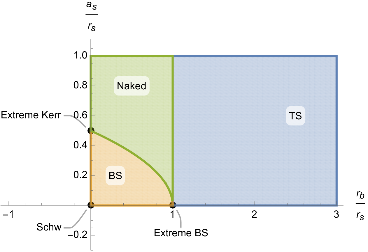
Figure 1: The phase diagram for RTS’s in terms of the dimensionless ratios $r_{b}/r_{s}$ & $a_{s}/r_{s}$. The static case is recovered by projecting onto $t_{2}=0$, while the usual Kerr string case correponds to the $t_{1}=0$ line. The black string and naked singularity phases are separated by an arc of parabola setting the bound on the rotation parameter $a_{s}$ as to avoid over-rotation. The extreme black string plays the role of a triple point in the phase diagram.

Note that the $a\to 0$ limit of (3.4) boils down to the static Horowitz-Strominger black string Horowitz:1991cd in (2.2) when $r_{s}>r_{b}$ or to the Bah-Heidmann Topological Star Bah:2020ogh when $r_{b}>r_{s}$. A first advantage of the parametrization we are using is that now the solution can be analytically continued for all values of $r_{s}$ and $r_{b}$, which is precisely what we need to do in order to describe a rotating topological soliton. As a bonus, it makes explicit the symmetry of the metric under the following transformations,

$$\begin{array}[]{lll}\left(t,y\right)\ \leftrightarrow\ \left(iy,it\right)\ ,&\left(r_{s},r_{b}\right)\ \leftrightarrow\ \left(r_{b},r_{s}\right)\ ,&\left(a_{s},a_{b}\right)\ \leftrightarrow\ \left(ia_{b},ia_{s}\right)\ ,\end{array}$$ (3.6)

which keep the metric and gauge field real. As in the static case, the solution (3.4) can be viewed as a superposition between a Lorentzian and a Euclidean Kerr solution, supported by a magnetic flux. Indeed, Lorentzian, Euclidean Kerr and the static black string/Topological Star solutions all appear as different limits of (3.4):

• $r_{s}\,=\,r_{b}\,=\,0:\leavevmode\nobreak\ \mathbb{R}^{1,4}$ written in oblate coordinates.

• $r_{b}\,=\,a_{b}\,=\,0$: Kerr${}_{4}\times S^{1}_{y}$ (Schw${}_{4}\times S^{1}_{y}$ when $a_{s}=0$).

• $r_{s}\,=\,a_{s}\,=\,0$: EKerr${}_{4}\times\mathbb{R}_{t}$ (ESchw${}_{4}\times\mathbb{R}_{t}$ when $a_{b}=0$).

• $a_{s}\,=\,a_{b}\,=\,0,r_{s}\geq r_{b}$: Horowitz-Strominger black string Horowitz:1991cd .

• $a_{s}\,=\,a_{b}\,=\,0,r_{b}>r_{s}$: static Bah-Heidmann Topological Star Bah:2020ogh .

In what follows we consider the case in which none of the parameters $r_{s,b}$ and $a_{s,b}$ vanishes, and investigate the different phases of the solution. The latter fall into three classes, depending on whether space terminates on a curvature singularity (naked or surrounded by a horizon) or a smooth cap. Denoting by $r_{\pm}$ the roots of $\Delta(r)$, we find

$$r_{\pm}\,=\,\frac{r_{b}+r_{s}}{2}\,\pm\,\sqrt{\left(\frac{r_{b}-r_{s}}{2}\right)^{2}-a^{2}}\,,$$ (3.7)

recalling that

$$a^{2}\,=\,a_{s}^{2}-a_{b}^{2}\,=\,a_{s}^{2}\left(1-\frac{r_{b}}{r_{s}}\right)\,=\,-a_{b}^{2}\left(1-\frac{r_{s}}{r_{b}}\right)\quad{\rm or}\quad a_{s}^{2}\,=\,-{a^{2}r_{s}\over r_{b}-r_{s}}\>,\>a_{b}^{2}\,=\,-{a^{2}r_{b}\over r_{b}-r_{s}}\quad.$$ (3.8)

Then, we have that $a^{2}$ is positive for $r_{s}>r_{b}$. This corresponds to the case studied in Compere:2009zh , in which space ends on a curvature singularity, either naked or surrounded by two horizons at $r_{\pm}$, according to the sign of the quantity under the square root. For $r_{b}>r_{s}$, instead, we show below that the geometry smoothly ends at $r_{+}$, which now represents a cap instead of an event horizon. Thus, this phase describes a horizonless topological soliton. A concise summary of the different phases is the following (see figure 1 and section 4.1 for a detailed discussion of the phase diagram):

• Naked singularity (NS): $r_{s}\,>\,r_{b}$ , $a^{2}>({\textstyle\frac{r_{s}-r_{b}}{2}})^{2}$.

• Rotating black string (RBS): $r_{s}\,>\,r_{b}\,$, $0<a^{2}\leq({\textstyle\frac{r_{s}-r_{b}}{2}})^{2}$.

• Rotating Topological Star (RTS): $r_{b}\,>\,r_{s}\,$, $a^{2}<0$.

• Extreme rotating black string (ERBS): $r_{s}\,=\,r_{b}$ , $a^{2}=0$.

Because of the constraint (3.3), the general solution has only three independent parameters, which can be taken to be $r_{s},r_{b}\in[0,\infty)$, and one between $a^{2},a_{s}^{2},a_{b}^{2}\in(-\infty,\infty)$. Moreover, in the BS and RTS phases, where $r_{\pm}$ are real, the general solution can be alternatively described in terms of $r_{s},r_{b}$ and $r_{+}$. The explicit expression of the rotation parameters in terms of these variables is

$$a_{s,b}\,=\,\sqrt{{\left(r_{+}-r_{b}\right)\left(r_{+}-r_{s}\right)r_{s,b}\over r_{b}-r_{s}}}\,,\hskip 28.45274pta^{2}\,=\,-\left(r_{+}-r_{b}\right)\left(r_{+}-r_{s}\right)\,.$$ (3.9)

Let us study in more detail the RBS and RTS phases and comment on ERBS at the very end.

3.2 Rotating black strings

This case has been already analyzed in Compere:2009zh , so we keep the discussion brief. Our goal here is to emphasize those aspects which will be useful when studying the solution in the topological soliton regime. As already stated, the rotating black string regime corresponds to

$$r_{s}\,>\,r_{b}\,,\hskip 28.45274pt0<a^{2}\leq({\textstyle\frac{r_{s}-r_{b}}{2}})^{2}\,,$$ (3.10)

which together with (3.7) implies

$$r_{s}>r_{+}>r_{b}\,.$$ (3.11)

The hypersurface $r=r_{+}$ is a Killing horizon for the following Killing vector,

$$\zeta\,=\,\partial_{t}+\zeta^{\phi}\,\partial_{\phi}+\zeta^{y}\,\partial_{y},$$ (3.12)

where

$$\zeta^{\phi}\,=\,\ \frac{r_{s}{-}r_{+}}{a_{s}\,r_{s}}\,=\,\sqrt{\frac{\left(r_{s}{-}r_{b}\right)\left(r_{s}{-}r_{+}\right)}{r_{s}^{3}\left(r_{+}{-}r_{b}\right)}}\,,\hskip 7.11317pt\quad\zeta^{y}\,=\,-\frac{a_{b}\,r_{b}}{a_{s}\,r_{s}}\frac{r_{s}{-}r_{+}}{r_{+}{-}r_{b}}\,=\,{-}\left(\frac{r_{b}}{r_{s}}\right)^{3/2}\frac{r_{s}{-}r_{+}}{r_{+}{-}r_{b}}\,.$$ (3.13)

To study the geometry near the horizon, it is convenient to introduce the coordinates

$$\tilde{t}\,=\,t\,,\hskip 28.45274pt{\tilde{\phi}}\,=\,{\tilde{\phi}}-\zeta^{\phi}\,t\,,\hskip 28.45274pt\tilde{y}\,=\,y-\zeta^{y}\,t\,,\hskip 28.45274pt\varrho^{2}\equiv 4\left(r-r_{+}\right)\,,$$ (3.14)

in terms of which the above Killing vector becomes simply $\zeta\,=\,\partial_{\tilde{t}}$. The metric at leading order in $\varrho$ is given by

$$\mathrm{d}s^{2}\,=\,\frac{\Sigma_{+}}{2r_{+}-r_{b}-r_{s}}\left(-\kappa^{2}\varrho^{2}\mathrm{d}{\tilde{t}}^{2}+\mathrm{d}\varrho^{2}\right)+\mathrm{d}s^{2}_{\cal H}\,,$$ (3.15)

where $\Sigma_{+}\equiv\Sigma\left(r_{+}\right)$,

$$\kappa^{2}\,=\,\frac{(r_{s}-r_{b})\left(2r_{+}-r_{b}-r_{s}\right)^{2}}{4\left(r_{+}-r_{b}\right)^{2}r_{s}^{3}}\,$$ (3.16)

is the square of the surface gravity and

$$\mathrm{d}s^{2}_{\cal H}\,= \frac{\Sigma_{+}\,\mathrm{d}\chi^{2}}{1-\chi^{2}}+\frac{\left(1-\chi^{2}\right)\,F_{\cal H}\left(\chi\right)}{\Sigma_{+}}\,\mathrm{d}{\tilde{\phi}}^{2}-\left(1-\frac{G_{\cal H}\left(\chi\right)}{\left(r_{s}-r_{b}\right)\Sigma_{+}^{2}}\right)\mathrm{d}{\tilde{y}}^{2}$$ (3.17)

$$+\frac{2r_{b}\left(1-\chi^{2}\right)}{\Sigma_{+}^{2}}\sqrt{\frac{r_{b}\left(r_{+}-r_{b}\right)\left(r_{+}-r_{s}\right)}{r_{b}-r_{s}}}\left[r_{+}^{3}-\left(r_{+}-r_{b}\right)\left(r_{+}-r_{s}\right)\chi^{2}\right]\mathrm{d}{\tilde{y}}\,\mathrm{d}{\tilde{\phi}}\,$$

is the induced metric at the horizon. The functions ${F}_{\cal H}$ and $G_{\cal H}$ are explicitly given by

$$F_{\cal H}(\chi)\,= \left(r_{+}\,r_{b}+r_{+}\,r_{s}-r_{s}\,r_{b}\right)^{2}-\frac{r_{s}\,r_{b}\,r_{+}^{2}\,\left(r_{+}-r_{b}\right)\left(r_{+}-r_{s}\right)\left(1-\chi^{2}\right)}{\Sigma_{+}},$$ (3.18)

$$G_{\cal H}(\chi)\,= r_{+}^{3}r_{b}\left(r_{s}-r_{b}\right)-r_{b}\left(r_{+}-r_{b}\right)\left(r_{+}-r_{s}\right)\left(r_{+}\,r_{b}-r_{+}\,r_{s}-r_{s}\,r_{b}\right)\chi^{2}\,.$$

The near-horizon metric (3.15) is Rindler${}_{2}\times S^{2}\times S^{1}$. The Rindler factor (which characterizes the near-horizon geometry of non-extremal black holes) is parametrized by the coordinates $t$ and $\varrho$; slices of the horizon at constant $t$ have $S^{2}\times S^{1}$ topology, with the $S^{1}$ being parametrized by the coordinate $y$, which is assumed to be compact. The $S^{1}$ never shrinks outside the horizon, and has finite size at infinity, where the solution tends to ${\mathbb{R}}^{1,3}\times S^{1}$. We conclude by observing the following property,

$$F_{\cal H}\left(\pm 1\right)\,=\,\Sigma^{2}_{+}\left(\pm 1\right)\,,$$ (3.19)

which ensures regularity of the metric (3.17) at the poles of the $S^{2}$.

3.3 Rotating Topological Stars

Next, we consider the topological soliton regime,

$$r_{b}\,>\,r_{s}\hskip 28.45274pt\Rightarrow\hskip 28.45274pta^{2}<0\,.$$ (3.20)

Taking into account (3.7), the above implies

$$r_{+}>r_{b}>r_{s}\,.$$ (3.21)

Contrarily to the RBS case, the hypersurface $r=r_{+}$ no longer corresponds to an event horizon, but rather to the locus where an $S^{1}$ shrinks to zero size, as we now show.

Regularity at the cap.

Consider the Killing vector

$$\xi\,=\partial_{y}+\xi^{\phi}\,\partial_{\phi}+\xi^{t}\,\partial_{t}\,,$$ (3.22)

where

$$\xi^{\phi}\,=\,-\frac{r_{+}-r_{b}}{a_{b}\,r_{b}}\,=\,-\sqrt{(r_{+}-r_{b})(r_{b}-r_{s})\over r_{b}^{3}(r_{+}-r_{s})}\,,\hskip 7.11317pt\xi^{t}\,=\,\ \frac{a_{s}\,r_{s}}{a_{b}\,r_{b}}\,\frac{r_{+}-r_{b}}{r_{+}-r_{s}}\,=\,\frac{r_{s}^{3/2}(r_{+}-r_{b})}{r_{b}^{3/2}(r_{+}-r_{s})}\,.$$ (3.23)

This is proportional to the generator of the horizon in (3.12) and (3.13), which makes it evident that its norm also vanishes at $r=r_{+}$,

$$g_{\mu\nu}\xi^{\mu}\xi^{\nu}|_{r_{+}}\,=\,0\,.$$ (3.24)

Contrarily to the black string case, $\xi$ is spacelike rather than timelike near $r\,=\,r_{+}$. This fact, together with the symmetry (3.6), strongly motivates us to introduce the following coordinates,

$$t^{\prime}\,=\,t-\xi^{t}\,y\,,\hskip 28.45274pt\phi^{\prime}\,=\,\phi-\xi^{\phi}\,y\,,\hskip 28.45274pty^{\prime}\,=\,\,y\,,\hskip 28.45274pt\varrho^{2}\,=\,4(r-r_{+})\,,$$ (3.25)

which are adapted to the isometry generated by $\xi$. In terms of them, this Killing vector simply becomes $\xi\,=\,\partial_{y^{\prime}}$ and the metric near the cap, at leading order in $\varrho$, becomes

$$\mathrm{d}s^{2}\,=\,\frac{\Sigma_{+}}{2r_{+}-r_{b}-r_{s}}\left(\mathrm{d}\varrho^{2}+{\textstyle\frac{\varrho^{2}}{R_{y}^{2}}}\,\,\mathrm{d}y^{\prime 2}\right)+\mathrm{d}s^{2}_{\rm cap}\,,$$ (3.26)

with

$$R_{y}=\frac{2\,r_{b}^{3/2}\left(r_{+}-r_{s}\right)}{\sqrt{r_{b}-r_{s}}\left(2r_{+}-r_{b}-r_{s}\right)}\,,$$ (3.27)

and

$$\mathrm{d}s^{2}_{\rm{cap}}\,= -\left(1-\frac{G_{\rm cap}(\chi)}{\left(r_{b}-r_{s}\right)\Sigma_{+}^{2}}\right){\mathrm{d}t^{\prime}}^{2}+\frac{\Sigma_{+}\,\mathrm{d}\chi^{2}}{1-\chi^{2}}+\frac{\left(1-\chi^{2}\right){F}_{\rm cap}(\chi)}{\Sigma_{+}}{\mathrm{d}\phi^{\prime}}^{2}$$ (3.28)

$$-\frac{2r_{s}\left(1-\chi^{2}\right)}{\Sigma_{+}^{2}}\sqrt{\frac{r_{s}\left(r_{+}-r_{b}\right)\left(r_{+}-r_{s}\right)}{r_{b}-r_{s}}}\left[r_{+}^{3}-\left(r_{+}-r_{b}\right)^{2}\left(r_{+}-r_{s}\right)\chi^{2}\right]\,\mathrm{d}t^{\prime}\,\mathrm{d}\phi^{\prime}\,,$$

is the induced metric at the cap, which has ${\mathbb{R}}\times S^{2}$ topology. The functions $F_{\rm cap}(\chi)$ and $G_{\rm cap}(\chi)$ are given by

$${F}_{\rm cap}\left(\chi\right)\,= F_{\cal H}(\chi)\,=\,\left(r_{+}\,r_{s}+r_{+}\,r_{b}-r_{s}\,r_{b}\right)^{2}-\frac{r_{s}\,r_{b}\,r_{+}^{2}\,\left(r_{+}-r_{b}\right)\left(r_{+}-r_{s}\right)\left(1-\chi^{2}\right)}{\Sigma_{+}}\,,$$ (3.29)

$$G_{\rm{cap}}(\chi)\,= r_{+}^{3}\,r_{s}\left(r_{b}-r_{s}\right)+r_{s}\left(r_{b}-r_{+}\right)\left(r_{+}-r_{s}\right)\left(r_{+}\,r_{b}-r_{+}\,r_{s}+r_{b}\,r_{s}\right)\chi^{2}\,.$$

Regularity of the near-cap metric (3.26) requires the following identifications of the coordinates,

$$(\phi^{\prime},y^{\prime})\sim(\phi^{\prime}+2\pi,y^{\prime})\sim(\phi^{\prime},y^{\prime}+2\pi R_{y})\,,$$ (3.30)

with the second implying the absence of conical singularities in the ${\mathbb{R}}^{2}$ parametrized by the coordinates $\varrho$ and $y^{\prime}$.

The asymptotic geometry.

Having analyzed the geometry near $r=r_{+}$, let us consider now the geometry at infinity. The metric (3.4) always asymptotes to flat spacetime,

$$\mathrm{d}s^{2}\,=\,-\mathrm{d}t^{2}+\mathrm{d}r^{2}+r^{2}\left(\mathrm{d}\theta^{2}+\sin^{2}\theta\,\mathrm{d}\phi^{2}\right)+\mathrm{d}y^{2}\,+\dots\,,$$ (3.31)

where the dots denote subleading terms in the $r\to\infty$ limit. Contrarily to what happens for the RBS, the coordinates $t,\phi,y$ now satisfy twisted periodic identifications, inherited from (3.30),

$$\left(t,\phi,y\right)\sim\left(t,\phi+2\pi,y\right)\,\sim\left(t+2\pi R_{y}\,\xi^{t},\phi+2\pi R_{y}\,\xi^{\phi},y+2\pi R_{y}\right)\,,$$ (3.32)

involving also the time coordinate. This can be remedied by boosting the solution along the $y$ direction with velocity $\xi^{t}$,

$$\hat{t}\,=\,\frac{t-\xi^{t}\,y}{\sqrt{1-\xi^{t}{}^{2}}}\,,\hskip 28.45274pt\hat{y}\,=\,\frac{y-\xi^{t}\,t}{\sqrt{1-\xi^{t}{}^{2}}}\,.$$ (3.33)

Notice that $\xi^{t}$, given in (3.23), satisfies $0<\xi^{t}<1$ in the soliton regime (3.21). Clearly, the boost leaves invariant the asymptotic metric (3.31), but has the advantage that when going once along the circle parametrized by $\hat{y}$, the time coordinate $\hat{t}$ no longer shifts. Indeed, the identifications (3.32) become

$$\left(\phi,\hat{y}\right)\sim\left(\phi+2\pi,\hat{y}\right)\,\sim\left(\phi+2\pi R_{y}\,\xi^{\phi},\hat{y}+2\pi R_{y}\sqrt{1-\xi^{t}{}^{2}}\right)\,.$$ (3.34)

Furthermore, the Killing vector (3.22) whose orbits generate the $S^{1}$ shriking at $r=r_{+}$ can be written in terms of the new coordinates as a linear combination of the two available U(1) isometries

$$\xi\,=\,\sqrt{1-\xi^{t}{}^{2}}\,\partial_{\hat{y}}+\xi^{\phi}\,\partial_{\phi}\,.$$ (3.35)

The identifications (3.34) become untwisted when the quantization condition $R_{y}\,\xi^{\phi}\in{\mathbb{Z}}$ is satisfied. This is what one would like to impose. Unfortunately, this condition does not admit real solutions in the rotating case. Nevertheless, we can relax it by imposing instead

$$R_{y}\,\xi^{\phi}\,=\,-{h\over q}\,,$$ (3.36)

where $h$ and $q$ are co-prime positive integers such that $q>h>0$. This condition implies that we come back to the same point after going $q$ times along the $\hat{y}$-circle. It is also equivalent to demanding that the orbits of $\xi$ are not dense in the torus generated by $\partial_{\hat{y}}$ and $\partial_{\phi}$ Gibbons:1979xm . In this case the asymptotic geometry is a freely acting $\mathbb{Z}_{q}$ orbifold of $\mathbb{R}^{1,3}\times S^{1}$. The action of ${\mathbb{Z}}_{q}$ is such that

$$\left(\phi,\hat{y}\right)\to\left(\phi+\frac{2\pi h}{q},\hat{y}+{2\pi R_{S^{1}}\over q}\right)\,,$$ (3.37)

where

$$R_{S^{1}}\,=\,qR_{y}\sqrt{1-\xi^{t}{}^{2}}\,.$$ (3.38)

Notice that the requirement (3.36) boils down to a quantization condition on the angular momentum,

$$a^{2}\,=\,-{h^{2}(r_{b}-r_{s})^{2}\over 4\left(q^{2}-h^{2}\right)}\,,\hskip 28.45274pth<q\,.$$ (3.39)

Finally, plugging this into (3.38), one finds the following constraint relating $R_{S^{1}}$, $r_{s}$ and $r_{b}$:

$$R_{S^{1}}^{2}\,=\,{c_{+}\,r_{b}^{3}-c_{-}r_{s}^{3}\over r_{b}-r_{s}}\,,$$ (3.40)

where

$$c_{\pm}\,=\,2q^{2}-h^{2}\pm 2\sqrt{q^{2}-h^{2}}\,.$$ (3.41)

In the static limit $h\to 0,q\to 1$, (3.40) correctly reduces to the result in Bah:2020ogh , namely

$$R^{2}_{S^{1}}\,=\,\frac{4\,r_{b}^{3}}{r_{b}-r_{s}}\,.$$ (3.42)

Note in particular that $R_{S^{1}}$ is always larger than $r_{s}$. As a matter of fact, $R_{S^{1}}/r_{s}$ has an absolute minimum at $r_{b}\,=\,3r_{s}/2$, where it takes the value $R_{S^{1}}/r_{s}\,=\,3\sqrt{3}\approx 5.2$. This feature persists in the rotating case, as we show in Fig. 2. This tells us that there is no separation of scales between the size of the $S^{1}$ and the would-be horizon scale, $r_{+}$.

Hence, once the boundary data ($R_{S^{1}},h,q$) are fixed, the solution has just one independent continuous parameter: the mass (or, equivalently, $r_{s}$), which is computed in section 3.5. Indeed, the dimensionless ratios $r_{c}/r_{s}$ and $r_{b}/r_{s}$ are fixed by (3.39) and (3.40). This is equivalent to saying that the magnetic charge and angular momentum are fixed in terms of the boundary data and the mass.

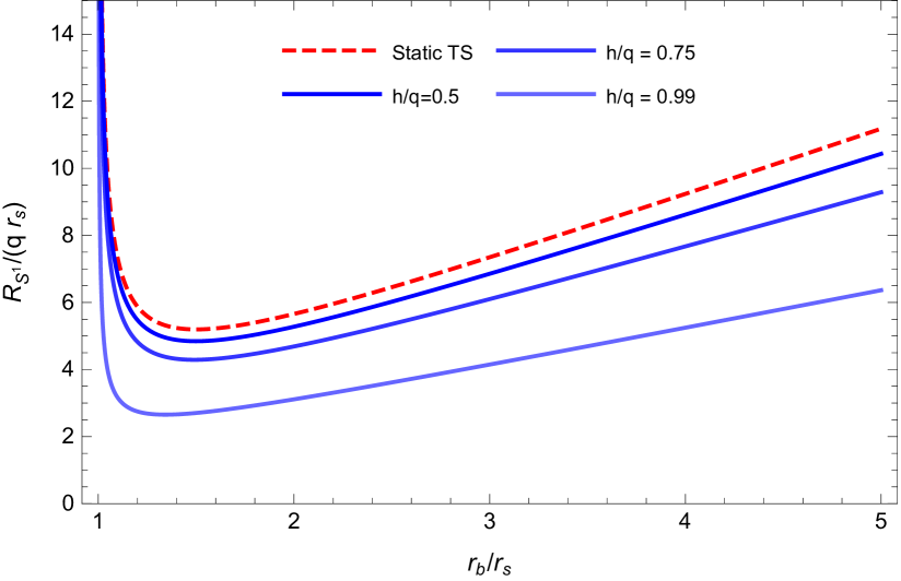
Figure 2: $\frac{R_{S^{1}}}{q\,r_{s}}$ as a function of $\frac{r_{b}}{r_{s}}$ for different values of $\frac{h}{q}$.

Absence of an ergoregion.

In pure General Relativity, spinning compact objects featuring an ergoregion without an event horizon are known to be unstable Friedman:1978ygc , since physical negative-energy states existing inside the ergoregion are energetically favorable to cascade toward even more negative states. As shown in Cardoso:2005gj , these ‘ergoregion instabilities’ affect other non-supersymmetric smooth horizonless geometries, such as JMaRT Jejjala:2005yu , that also suffer from charge instabilities Bianchi:2023rlt .

Here we show that no potential issue of this kind may take place in our solutions since the Killing vector $\partial_{\hat{t}}$ is everywhere timelike. Its norm, given by the $\hat{t}\hat{t}$ component of the metric, reads

$$-g_{\hat{t}\hat{t}}\,=\,1+\frac{\xi^{t}{}^{2}r_{b}-r_{s}}{1-\xi^{t}{}^{2}}\,\frac{r}{\Sigma}+\frac{\left(a_{s}-\xi^{t}a_{b}\right)^{2}}{1-\xi^{t}{}^{2}}\,\frac{r_{s}r_{b}\chi^{2}}{\Sigma^{2}}\,.$$ (3.43)

The last term is manifestly positive, so we just have to show that the remaining ones be positive as well. To this aim, we recall that in the soliton regime $r\geq r_{+}$ and $a^{2}<0$, which implies that $0<\Sigma<r^{2}$, and $\xi^{t}<1$. Then,

$$1+\frac{\xi^{t}{}^{2}r_{b}-r_{s}}{1-\xi^{t}{}^{2}}\,\frac{r}{\Sigma}>1+\frac{\xi^{t}{}^{2}r_{b}-r_{s}}{1-\xi^{t}{}^{2}}\,\frac{1}{r}>\left(1-\xi^{t}{}^{2}\right)\frac{r-r_{b}}{r}>0\,,$$ (3.44)

where we used the fact that space ends at $r=r_{+}>r_{b}>r_{s}$. Thus, we conclude that the would-be ergoregion is not part of the RTS spacetime.

Absence of closed timelike curves (CTC).

In order to check the absence of CTC in our geometry, we follow Elvang:2004ds , where it is argued that the positive-definiteness of the induced metric on a Cauchy slice at constant $\hat{t}$ ensures the absence of CTC in a region where $\partial_{\hat{t}}$ is timelike. We emphasize that although the authors apply this in a supersymmetric context, the argument holds whenever the latter condition is satisfied. As we showed in (3.43), in our geometry $\partial_{\hat{t}}$ is always timelike. Hence, we just have to check that the induced metric on $\hat{t}\,=\,\rm{constant}$ hypersurface is positive definite.

Given the form of the metric, this reduces to a two-dimensional problem, since the $r-\chi$ part is automatically positive-definite. The relevant two-dimensional metric is then the following,

$$\mathrm{d}s^{2}_{\phi,\hat{y}}\,=\,g_{\hat{y}\hat{y}}\left(\mathrm{d}\hat{y}+\frac{g_{\hat{y}\phi}}{g_{\hat{y}\hat{y}}}\mathrm{d}\phi\right)^{2}+\frac{\cal D}{g_{\hat{y}\hat{y}}}\,{\mathrm{d}\phi}^{2}\,,$$ (3.45)

where $\cal D$ is the determinant. Thus, the metric is positive-definite if

$$g_{\hat{y}\hat{y}}>0\,,\hskip 28.45274pt{\cal D}>0\,.$$ (3.46)

In order to demonstrate the strict inequality one has to stay away from the poles $\chi\,=\,\pm 1$, where we already know that regularity imposes that both $\cal D$ and $g_{\hat{y}\phi}$ vanish. Similarly, we know that $g_{\hat{y}\hat{y}}$ must vanish at the poles of the $S^{2}$ at $r=r_{+}$, since these correspond to the fixed points of the isometry $\partial_{\hat{y}}$. This can be deduced from (3.35), where we showed that $\partial_{\hat{y}}$ is a linear combination of $\partial_{y^{\prime}}$ and $\partial_{\phi}$ which vanish, respectively, at $r=r_{+}$ and $\chi=\pm 1$.

A sketch of the proof is the following. The expression for $\cal D$ is of the form,

$${\cal D}\,=\,\frac{1-\chi^{2}}{r_{s}^{2}\left(1-\xi^{t}{}^{2}\right)\Sigma}\left({\cal D}_{(0)}+\left(1-\chi^{2}\right){\cal D}_{(1)}\right)\,,$$ (3.47)

where ${\cal D}_{(0)}$ and ${\cal D}_{(1)}$ are functions of $r$, whose explicit expression is not displayed, as it is somewhat lengthy and unilluminating. The important point is that ${\cal D}_{(1)}$ is manifestly positive, which implies

$${\cal D}\,>\,\frac{\left(1-\chi^{2}\right){\cal D}_{(0)}}{r_{s}^{2}\left(1-\left(\xi^{t}\right)^{2}\right)\Sigma}\,.$$ (3.48)

Then one can check, with the help of the Reduce command of Mathematica, that ${\cal D}_{(0)}>0$. For $g_{\hat{y}\hat{y}}$ one can follow a similar strategy. First, we write it as

$$g_{\hat{y}\hat{y}}\,=\,\frac{1}{r_{s}^{2}\left(1-\left(\xi^{t}\right)^{2}\right)\Sigma^{2}}\left[{\cal G}_{(0)}+{\cal G}_{(1)}\left(1-\chi^{2}\right)+{\cal G}_{(2)}\left(1-\chi^{2}\right)^{2}\right]\,,$$ (3.49)

and then show that the functions ${\cal G}_{(0)}$, ${\cal G}_{(1)}$ and ${\cal G}_{(2)}$, which only depend on $r$, are positive (except at the fixed points of $\partial_{\hat{y}}$). This ensures there are no CTC in the RTS geometry.

3.4 Extreme rotating black strings

We notice that the NS and RTS regions are divided by a continuous line of solutions (see figure 1) corresponding to the choice

$$r_{+}\,=\,r_{b}\,=\,r_{s}\,,\,\hskip 28.45274pta_{b}\,=\,a_{s}\,,\hskip 28.45274pta^{2}\,=\,0\,,\\$$

whereby the functions $\Delta$ and $\Sigma$ simply reduce to

$$\Delta\,=\,(r-r_{s})^{2}\,,\hskip 28.45274pt\Sigma\,=\,r^{2}\ .$$ (3.50)

The corresponding form of the 5d metric becomes

$$\mathrm{d}s^{2}\,=\,\mathrm{d}s_{\mathrm{EBS}}^{2}\,-\,a_{s}^{2}r_{s}^{2}\frac{\chi^{2}}{r^{4}}(\mathrm{d}t-\mathrm{d}y)^{2}\,-\,2a_{s}\,r_{s}\frac{1-\chi^{2}}{r}(\mathrm{d}t-\mathrm{d}y)\mathrm{d}\phi\ ,$$ (3.51)

which could be understood as a one-parameter deformation of the extreme static black string solution, whose line element we denote by $\mathrm{d}s_{\mathrm{EBS}}^{2}$:

$$\mathrm{d}s_{\mathrm{EBS}}^{2}\,=\,f_{s}\left(-\mathrm{d}t^{2}+\mathrm{d}y^{2}\right)\,+\,\frac{\mathrm{d}r^{2}}{f_{s}^{2}}\,+\,r^{2}\mathrm{d}s_{S^{2}}^{2}\ ,$$ (3.52)

with $f_{s}\equiv\left(1-\dfrac{r_{s}}{r}\right)$. Introducing the coordinates

$$u\,=\,t-y\,,\hskip 28.45274ptv\,=\,t+y\,,$$ (3.53)

the metric and gauge field can be brought into the form

$$\mathrm{d}s^{2}\,= -f_{s}\,\mathrm{d}u\left(\mathrm{d}v+\frac{a_{s}^{2}r_{s}^{2}\chi^{2}}{r^{4}f_{s}}\mathrm{d}u+\frac{2a_{s}r_{s}\left(1-\chi^{2}\right)}{rf_{s}}\,\mathrm{d}\phi\right)\,+\,\frac{\mathrm{d}r^{2}}{f_{s}^{2}}\,+\,r^{2}\mathrm{d}s_{S^{2}}^{2}\,,$$ (3.54)

$$A\,= -\sqrt{3r_{s}r_{b}}\,\chi\left(\mathrm{d}\phi-\frac{a_{s}}{r^{2}}\,\mathrm{d}u\right)\,.$$

This solution possesses mass and angular momentum and exhibits a curvature singularity at $r=0$.

3.5 Five-dimensional charges

We are now ready to compute the five-dimensional charges of the BS and RTS solutions. These are given by the general formulae:

$${\cal M}\,=\,{3\over 4\kappa_{5}^{2}}\int\limits_{\Sigma_{\infty}}\star\mathrm{d}K^{\sharp}_{(t)}\,,\hskip 28.45274pt{\cal J}\,=\,{1\over 2\kappa_{5}^{2}}\int\limits_{\Sigma_{\infty}}\star\mathrm{d}K^{\sharp}_{(\phi)}\,,\hskip 28.45274pt{\cal P}\,=\,{1\over 2\kappa_{5}^{2}}\int\limits_{\Sigma_{\infty}}\star\mathrm{d}K^{\sharp}_{(y)}\,,$$ (3.55)

where $K^{\sharp}_{(i)}=g_{i\mu}\,\mathrm{d}x^{\mu}$ are the one-forms associated to the three Killing vectors $K_{(i)}$ generating the isometries of the solutions, and $\Sigma_{\infty}$ a spatial cross-section of the asymptotic boundary. This is summarized in the table below.

$$\begin{array}[]{c|c|c|c|c}&\leavevmode\nobreak\ \leavevmode\nobreak\ K_{(t)}\nobreak\leavevmode\nobreak\leavevmode&\leavevmode\nobreak\ \leavevmode\nobreak\ K_{(\phi)}\nobreak\leavevmode\nobreak\leavevmode&\leavevmode\nobreak\ \leavevmode\nobreak\ K_{(y)}\nobreak\leavevmode\nobreak\leavevmode&\Sigma_{\infty}\\ \hline\cr{\rm RBS}&\partial_{t}&\partial_{\phi}&\partial_{y}&S^{2}\times S^{1}\\ {\rm RTS}&\partial_{\hat{t}}&\partial_{\phi}&\partial_{\hat{y}}&\left(S^{2}\times S^{1}\right)/\mathbb{Z}_{q}\\ \end{array}$$

Charges for the rotating black string.

The mass and angular momentum of the RBS can be extracted from the asymptotics of the $g_{tt}$ and $g_{t\phi}$ components of the metric. One finds

$${\cal M}\,= \frac{3V_{S^{2}\times S^{1}}}{4\kappa^{2}_{5}}\lim_{r\to\infty}\left(-r^{2}\,\partial_{r}g_{tt}\right)\,=\,\frac{3V_{S^{2}\times S^{1}}}{4\kappa^{2}_{5}}\,r_{s}\,,$$ (3.56)

$${\cal J}\,= \frac{V_{S^{2}\times S^{1}}}{2\kappa^{2}_{5}}\lim_{r\to\infty}\left(r^{2}\,{\partial_{r}g_{t\phi}\over 1-\chi^{2}}\right)\,=\,\frac{V_{S^{2}\times S^{1}}}{2\kappa_{5}^{2}}2a_{s}r_{s}\,,$$

where

$$V_{S^{2}\times S^{1}}\,=\,8\pi^{2}R_{S^{1}}\,.$$ (3.57)

The momentum charge ${\cal P}$ vanishes since $g_{ty}\,=\,{\cal O}\left(1/r^{4}\right)$.

Charges for the Rotating Topological Star.

Although the form of the solution is the same, the expressions for the charges of the topological soliton differ from the black string for two reasons. The first is the fact that the boundary is different, as we have explained in section 3.3. The second is the boost we have performed along the $y$ direction. This will give rise to a non-vanishing momentum charge ${\cal P}$, as can be seen from the asymptotic expansion of the metric:

$$\mathrm{d}s^{2} \,=\, -\left(1-\frac{r_{s}-\xi^{t}{}^{2}r_{b}}{1-\xi^{t}{}^{2}}\,\frac{1}{r}\right)\,\mathrm{d}\hat{t}^{2}+\left(1-\frac{r_{b}-\xi^{t}{}^{2}r_{s}}{1-\xi^{t}{}^{2}}\,\frac{1}{r}\right)\,\mathrm{d}\hat{y}^{2}+\mathrm{d}r^{2}+r^{2}\mathrm{d}s^{2}_{S^{2}}$$

$$-\frac{2\xi^{t}\left(r_{b}{-}r_{s}\right)}{1-\xi^{t}{}^{2}}\frac{1}{r}\,\mathrm{d}\hat{t}\,\mathrm{d}\hat{y}+2\frac{1-\chi^{2}}{r}\left[\frac{a_{b}r_{b}\xi^{t}-a_{s}r_{s}}{\sqrt{1-\xi^{t}{}^{2}}}\,\mathrm{d}\hat{t}\,\mathrm{d}\phi{+}{a_{b}r_{b}{-}a_{s}r_{s}\xi^{t}\over\sqrt{1{-}\xi^{t}{}^{2}}}\mathrm{d}\hat{y}\,\mathrm{d}\phi\right]+\ldots\,$$

where

$$\mathrm{d}s^{2}_{S^{2}}=\frac{\mathrm{d}\chi^{2}}{1-\chi^{2}}+\left(1-\chi^{2}\right)\,\mathrm{d}\phi^{2}\,,$$ (3.59)

is the metric of the round $S^{2}$ and the dots denote $1/r^{2}$-corrections. From (3.55) one finds:

$${\cal M}\,= \frac{3V_{S^{2}\times S^{1}}}{4q\kappa^{2}_{5}}\lim_{r\to\infty}\left(-r^{2}\,\partial_{r}g_{\hat{t}\hat{t}}\right)\,=\frac{3V_{S^{2}\times S^{1}}}{4q\kappa_{5}^{2}}\frac{r_{s}-\xi^{t}{}^{2}r_{b}}{1-\xi^{t}{}^{2}}\,,$$ (3.60)

$${\cal J}\,= \frac{V_{S^{2}\times S^{1}}}{2q\kappa^{2}_{5}}\lim_{r\to\infty}\left(r^{2}\,{\partial_{r}g_{\hat{t}\phi}\over 1-\chi^{2}}\right)\,=\,\frac{V_{S^{2}\times S^{1}}}{2q\kappa_{5}^{2}}\,{a_{s}\,r_{s}{-}a_{b}\,r_{b}\,\xi^{t}\over\sqrt{1{-}\xi^{t}{}^{2}}}\,,$$

$${\cal P}\,= \,\frac{V_{S^{2}\times S^{1}}}{2q\kappa^{2}_{5}}\lim_{r\to\infty}\left(r^{2}\,{\partial_{r}g_{\hat{t}\hat{y}}\over 1-\chi^{2}}\right)\,=\,\frac{V_{S^{2}\times S^{1}}}{q\kappa_{5}^{2}}\,{\left(r_{b}{-}r_{s}\right)\xi^{t}\over 1{-}\xi^{t}{}^{2}}\,.$$

We conclude showing explicitly that the mass is positive, as it is not manifest from the above expression. However, using (3.23) we have that

$$r_{s}-\xi^{t}{}^{2}r_{b}\,=\,\frac{r_{s}}{\left(r_{+}-r_{s}\right)^{2}}\left[r_{b}^{2}\left(r_{+}-r_{s}\right)^{2}-r_{s}^{2}\left(r-r_{b}\right)^{2}\right]>0\,,$$ (3.61)

since $r_{+}>r_{b}>r_{s}>0$.

4 Dimensional reduction to four dimensions

In this section we perform the dimensional reduction of the RTS solution down to four dimensions. As discussed in Dowker:1995gb , there are two possibilities: either we reduce along $\xi$ or $\partial_{\hat{y}}$, given that both have closed orbits. Note that using (3.35), the latter can be written as

$$R_{S^{1}}\,\partial_{\hat{y}}\,=\,q\,R_{y}\,\xi-h\,\partial_{\phi}\,,$$ (4.1)

and recall that $\xi$ is $2\pi R_{y}$ periodic. Here we choose to reduce along $\partial_{\hat{y}}$, since the reduction along $\xi$ gives rise to a divergent Kaluza-Klein scalar at large $r$ Dowker:1995gb . Nevertheless, it is important to bear in mind that both possibilities are pathological, in the sense that both Killing fields have fixed points. This is telling us that the solution is genuinely five-dimensional. The reduction ansatz is:

$$\begin{array}[]{lcl}\mathrm{d}s^{2}&=&e^{\varphi}\,\mathrm{d}s_{4}^{2}\,+\,e^{-2\varphi}\,\left(\mathrm{d}\hat{y}+\mathcal{B}\right)^{2}\ ,\\[5.69054pt] A&=&\mathcal{A}\,+\,\alpha\,\left(\mathrm{d}\hat{y}+\mathcal{B}\right)\ ,\end{array}$$ (4.2)

with $\mathcal{A}$, $\mathcal{B}$ some one-forms in 4d. Assuming that all five-dimensional fields be $\hat{y}$-independent, the five-dimensional action (3.1) reduces to

$$S_{4}\,=\,\frac{1}{2\kappa_{4}^{2}}\int\mathrm{d}^{4}x\sqrt{-g}\,\bigg{[} R_{4}-\frac{3}{2}\left(\partial\varphi\right)^{2}-\frac{e^{2\varphi}}{2}\left(\partial\alpha\right)^{2}-\frac{e^{-\varphi}}{4}|F_{(2)}|^{2}-\frac{e^{-3\varphi}}{4}|G_{(2)}|^{2}$$ (4.3)

$$+\frac{\alpha}{2\sqrt{3}}\,\epsilon^{\mu\nu\rho\sigma}\,\left(F_{\mu\nu}F_{\rho\sigma}-\alpha F_{\mu\nu}G_{\rho\sigma}+\frac{\alpha^{2}}{3}G_{\mu\nu}G_{\rho\sigma}\right)\bigg{]}\ ,$$

where

$$\begin{array}[]{lll}F_{(2)}\,\equiv\,\mathrm{d}\mathcal{A}+\alpha\,\mathrm{d}\mathcal{B}\,,&G_{(2)}\,\equiv\,\mathrm{d}\mathcal{B}\,,&\kappa_{4}^{2}\,\equiv\,\dfrac{q\kappa_{5}^{2}}{2\pi R_{S^{1}}}\ .\end{array}$$ (4.4)

The 4d effective description couples the 4d metric, to two vector fields $(\mathcal{A},\mathcal{B})$ and a ‘complex’ axio-dilaton field consisting in the two real scalars $(\varphi,\alpha)$. The explicit form of the 4d metric may be directly read off from the reduction ansatz (4.2). Since the complete metric is quite involved, we will not display it explicitly. We can provide instead its asymptotic expansion for large $r$, which is undistinguisable from the Kerr metric:

$$\mathrm{d}s^{2}_{4}\,=\,-\left(1-\frac{2G_{4}M}{r}\right)\,\mathrm{d}{\hat{t}}^{2}-\frac{4G_{4}J\left(1-\chi^{2}\right)}{r}\,\mathrm{d}{\hat{t}}\,\mathrm{d}\phi+\left(1+\frac{2G_{4}M}{r}\right)\,\mathrm{d}r^{2}+r^{2}\,\mathrm{d}s^{2}_{S^{2}}+\dots\,,$$ (4.5)

with mass $M$ and angular momentum $J$ given in terms of the parameters by

$$M\,=\,\frac{2r_{s}+r_{b}+\xi^{t}{}^{2}\left(r_{s}+2r_{b}\right)}{4G_{4}\left(1-\xi^{t}{}^{2}\right)}\,,\hskip 28.45274ptJ\,=\,\frac{a_{s}\,r_{s}-a_{b}\,r_{b}\,\xi^{t}}{2G_{4}\sqrt{1-\xi_{t}^{2}}}\,.$$ (4.6)

Note that the expression for the mass differs (apart from a normalization factor) from the five-dimensional one in (3.60). The reason is that the 4d and 5d metrics are related by a conformal factor $e^{\varphi}$ (see (4.2)), which contributes to the mass as a consequence of the non-trivial profile of the Kaluza-Klein scalar. In addition, we further note that the mass is manifestly positive and reduces to the result of Bah:2020ogh in the static limit, whereby $\xi^{t}\to 0$.

Just as in the static case, the 4d geometry exhibits curvature singularities when the Kaluza-Klein scalar $\varphi$ diverges. From the explicit expression of the latter,

$$g_{\hat{y}\hat{y}}\,=\,e^{-2\varphi}\,=\,\frac{\chi^{2}r_{b}r_{s}\left(a_{b}-a_{s}\xi^{t}\right){}^{2}+r\Sigma\left(r_{b}-r_{s}\xi^{t}{}^{2}\right)+\Sigma^{2}\left(\xi^{t}{}^{2}-1\right)}{\Sigma^{2}\left(\xi^{t}{}^{2}-1\right)}\,,$$ (4.7)

one sees that $\varphi$ diverges along a curve in the $(r,\chi)$ plane, which is displayed in figure 3. This touches the north and south poles of the $S^{2}$ at the cap, which are the fixed points of ${\partial}_{\hat{y}}$. There, both the 4d Ricci scalar and the axionic kinetic energy diverge.

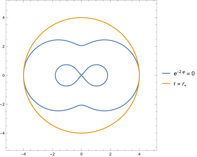
Figure 3: Curve in the $\left(x,y\right)\,=\,\left(r\chi,r\sqrt{1-\chi^{2}}\right)$ plane along which $e^{-2\varphi}$ vanishes. We have chosen the values $r_{+}\,=\,4$, $r_{b}=2$, $r_{s}=1$.

4.1 The phase diagram

We conclude this section by performing a more exhaustive analysis of the space of solutions. To this aim, it is convenient to introduce the two dimensionless quantities

$$t_{1}\ \equiv\ \frac{r_{b}}{r_{s}}\ ,\qquad t_{2}\ \equiv\ \frac{a_{s}}{r_{s}}\ .$$ (4.8)

In terms of these variables the largest root $r_{+}$ of $\Delta$ reads

$$\frac{r_{+}}{r_{s}}\,=\,{\textstyle\frac{1}{2}}\left[t_{1}+1+\,\sqrt{\left(t_{1}-1\right)\left(t_{1}-1+4t_{2}^{2}\right)}\right]\ .$$ (4.9)

Therefore, the space of solutions can be split into three main phases:

$$\begin{array}[]{lll}\ \begin{array}[]{cc}1>t_{1}>1-4t_{2}^{2}&\quad\textrm{NS}\\[5.69054pt] t_{1}<\left(1-4t_{2}^{2}\right)&\quad\textrm{RBS}\\[5.69054pt] t_{1}>1\ ,\ \forall\ t_{2}&\quad\textrm{RTS}\end{array}\end{array}$$ (4.10)

The corresponding phase diagram is depicted in figure 4. The horizontal $t_{1}$-axis represents the static black string/Topological Star line, while the Kerr black hole spans the vertical $t_{2}$-axis. We notice that the black string (BS) and the topological star (TS) phases are only connected through the extremal BS point, which represents a triple point for the phase diagram.

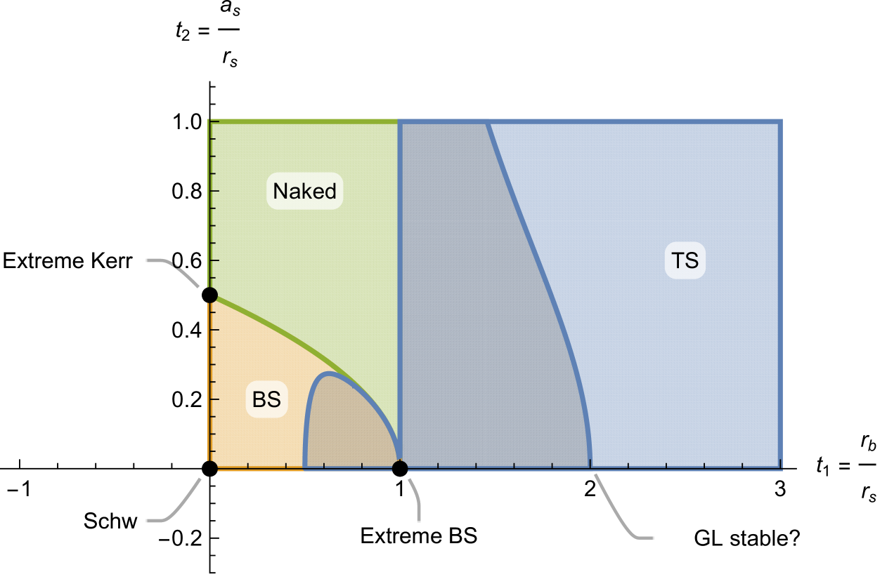
Figure 4: The phase diagram for RTS’s in terms of the dimensionless ratios $t_{1}$ & $t_{2}$. The shaded areas could represent the regions of GL stability.

Black string and extended solutions are known to suffer from Gregory-Laflamme (GL) instabilities Gregory:1993vy when the Kaluza-Klein radius is not small enough. This is certainly the case of black string solutions along the $t_{2}$-axis in the phase diagram. On the other hand static solutions with $t_{1}\neq 0$ Horowitz:1991cd ; Bah:2020ogh , although generically unstable, have been shown to be free of GL instabilities in the the two windows $r_{b}<r_{s}<2r_{b}$ and $r_{s}<r_{b}<2r_{s}$ Bena:2024hoh ; Miyamoto:2007mh , i.e. along the segment $t_{2}=0$ and ${\textstyle\frac{1}{2}}<t_{1}<2$. This suggests that rotating solutions continuously connected to this segment should be GL stable for $t_{2}$ small enough, i.e. for small enough rotation parameter. A rigorous proof of this expectation would require a direct calculation of QNM frequencies of all linear perturbations of the rotating metric, a challenging task that can be addressed by with recently proposed methods based on the duality with ${\cal N}=2$ supersymmetric gauge theories Aminov:2020yma ; Bianchi:2021xpr ; Bianchi:2021mft ; Bonelli:2021uvf ; Bonelli:2022ten ; Bianchi:2022qph ; Consoli:2022eey ; Bautista:2023kns ; Bianchi:2024zgn ; DiRusso:2024rgi ; Cipriani:2025ikx , but is beyond the scope of our present work. We will limit ourselves and observe that the interval of GL stabilty in the static case is bounded by the points $(t_{1},t_{2})=({\textstyle\frac{1}{2}},0),\leavevmode\nobreak\ (2,0)$ where the $P/M$ ratio between the magnetic charge and the four-dimensional mass is extremized. Indeed, plotting the level curves for the this ratio, one sees that the two threshold points for GL instability in the static case represent saddles of this function. These level curves are represented in figure 5, from which it appears very evident that the dashed black curves are boundaries between regions where the level curves are open and other which are closed. The regions below these dashed lines have therefore the charge/mass ratio in the allowed range and are candidate regions for GL stability. In particular, the ones corresponding to the shaded areas in figure 4 are also continuously connected to the stability window for the static case $t_{2}=0$. It may be worth mentioning that such a window tends to decrease in size once we increase the value of the rotation parameter $a_{s}$, as it is natural to expect.

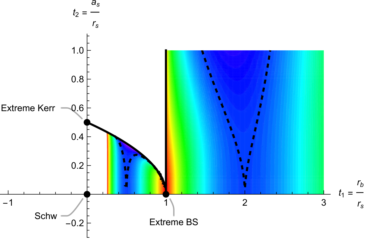
Figure 5: The level curves of the charge to mass ratio as a function of $t_{1}$ & $t_{2}$. The white region on the left has very low values which approach zero and cannot be represented in the same scale as the rest of our diagram. The black dashed lines separate closed and open level curves.

5 Geodetic Motion

In order to probe the RTS geometry, it is interesting to study geodetic motion of a massive spinless probe. Scalar perturbations in the RTS background will be discussed in section 6. Thanks to the three commuting isometries, one can conveniently describe the relevant dynamics in Hamilton form,

$${\cal H}\,=\,g^{\mu\nu}P_{\mu}P_{\nu}=-\mu^{2}\,.$$ (5.1)

where $g^{\mu\nu}$ is the inverse metric, $P_{\mu}=g_{\mu\nu}\dot{x}^{\nu}$ and $\mu$ is the mass of the probe. In particular

$$P_{r}={\Sigma\over\Delta}\dot{r}\quad,\quad P_{\chi}={\Sigma\over 1-\chi^{2}}\dot{\chi}$$ (5.2)

while $E=-P_{t}$, $J=P_{\phi}$ and $p=P_{y}$ are conserved momenta that we collectively denote by ${\cal I}_{a}$. After some algebra one finds

$$\Sigma[{\cal H}+\mu^{2}]=\Delta P_{r}^{2}+(1-\chi^{2})P_{\chi}^{2}+W(r,\chi;{\cal I}_{a})=0$$ (5.3)

where

$$W={N(r,\chi;{\cal I}_{a})\over\Delta(1-\chi^{2})}+\mu^{2}\Sigma$$ (5.4)

The numerator is a quartic polynomial in both $r$ and $\chi$ and is obviously quadratic in ${\cal I}_{a}$ and $\mu$ viz.

$$N(r,\chi;{\cal I}_{a})=A\Delta+B(r)(1-\chi^{2})+C\Delta(1-\chi^{2})^{2}$$ (5.5)

with

$$A=J^{2}\quad,\quad B(r)=\sum_{k=0}^{4}\beta_{k}r^{k}\quad,\quad C=-a^{2}(p^{2}-E^{2})$$ (5.6)

It is now clear that one can introduce a separation constant $K^{2}$, akin to Carter’s constant for geodetic motion in Kerr(-Newman) BH’s or in circular fuzzballs Bianchi:2017sds , and set

$$(1-\chi^{2})P_{\chi}^{2}+{J^{2}\over(1-\chi^{2})}-a^{2}(p^{2}-E^{2})(1-\chi^{2})+a^{2}\chi^{2}\mu^{2}=K^{2}-a^{2}(p^{2}-E^{2})$$ (5.7)

so that

$$(1-\chi^{2})P_{\chi}^{2}+{J^{2}\over(1-\chi^{2})}-a^{2}(E^{2}-p^{2}-\mu^{2})\chi^{2}=K^{2}$$ (5.8)

The radial Hamiltonian then becomes

$$\Delta P_{r}^{2}+{B(r)\over\Delta}+\mu^{2}r^{2}=-K^{2}+a^{2}(p^{2}-E^{2})$$ (5.9)

that can be put in the very neat form

$$P_{r}^{2}+Q_{R}=0$$ (5.10)

where

$$Q_{R}={N_{4}\over\Delta^{2}}+{\mu^{2}r^{2}\over\Delta}$$ (5.11)

with

$$N_{4}=B+[K^{2}-a^{2}(p^{2}-E^{2})]\Delta=\sum_{k=0}^{4}\gamma_{k}r^{k}$$ (5.12)

with

$$\gamma_{4}\,= p^{2}-E^{2}\,,\hskip 28.45274pt\gamma_{3}\,=\,-p^{2}r_{s}+E^{2}r_{b}\,,\hskip 28.45274pt\gamma_{2}\,=\,K^{2}-a^{2}\left(E^{2}-p^{2}\right)\,,$$ (5.13)

$$\gamma_{1}\,= a^{2}\left(p^{2}r_{b}-E^{2}r_{s}\right)+2J\left(Ea_{s}r_{s}-pa_{b}r_{b}\right)-K^{2}\left(r_{b}+r_{s}\right)\,,$$

$$\gamma_{0}\,= r_{s}r_{b}K^{2}-a^{2}\left(J^{2}-K^{2}\right)-2r_{s}r_{b}J\left(a_{s}E-a_{b}p\right)+\left(a_{s}r_{b}p-a_{b}r_{s}E\right)^{2}\,.$$

Geodesics are non planar in general. Planar ‘shear-free’ geodesics at $\chi=\chi_{0}$ exist for specific choices of $J$ and $K$ such that $P_{\chi}=0$

$$Q_{\chi}={J^{2}\over(1-\chi_{0}^{2})^{2}}-{K^{2}+a^{2}(E^{2}-p^{2}-\mu^{2})\chi_{0}^{2}\over 1-\chi_{0}^{2}}=0$$ (5.14)

and the polar angular ‘force’ vanish

$${dQ_{\chi}\over d\chi}|_{\chi=\chi_{0}}=0$$ (5.15)

It is easy to show that the equatorial plane $\chi_{0}=0$ is a solution of the shear-free condition if $J^{2}=K^{2}$. For ${\cal J}\sim a_{s}r_{s}{-}a_{b}r_{b}\xi^{t}>0$, $J=+K$ corresponds to co-rotating geodesics while the case $J=-K$ corresponds to counter-rotating geodesics.

Critical geodesics correspond to $P_{r}=0$ and $P_{r}^{\prime}=0$, they are non planar in general except for the equatorial ones.

Let us focus for simplicity on null geodesics in the equatorial plane with $p=0$ that characterize the light-rings Bianchi:2018kzy ; Bianchi:2020des ; Bacchini:2021fig ; Heidmann:2022ehn . In order to set the stage let’s recall that for static Top Stars, thanks to spherical symmetry, one can focus on equatorial null geodesics. To avoid a KK mass of the probe we put $P_{y}=0$.

The reduced metric is then simply

$$\mathrm{d}s^{2}=-f_{s}\mathrm{d}t^{2}+{\mathrm{d}r^{2}\over f_{s}f_{b}}+r^{2}\mathrm{d}\phi^{2}$$ (5.16)

Setting $E=-P_{t}=-f_{s}\dot{t}$ and $J=P_{\phi}=r^{2}\dot{\phi}$, the null Hamiltonian reads

$${\cal H}=f_{s}f_{b}P_{r}^{2}-{E^{2}\over f_{s}}+{J^{2}\over r^{2}}=0$$ (5.17)

Note that

$$\dot{r}=f_{s}f_{b}P_{r}$$ (5.18)

that vanishes for $P_{r}=0$ but also at $r=r_{b}$ ($r=r_{s}$ is not part of the geometry). Critical geodesics correspond to $\dot{r}=0$ and $F_{r}=0$. Setting $b=J/E$, for $r\neq r_{b}$ one has

$$P_{r}^{2}=-Q_{R}=0$$ (5.19)

with

$$Q_{R}={E^{2}\over(r-r_{s})^{2}(r-r_{b})}[b^{2}(r-r_{s})-r^{3}]=0\quad,\quad$$ (5.20)

and

$$Q_{R}^{\prime}={E^{2}\over(r-r_{s})^{2}(r-r_{b})}[b^{2}-3r^{2}]+E^{2}[b^{2}(r-r_{s})-r^{3}]{d(r-r_{s})^{-2}(r-r_{b})^{-1}\over dr}=0$$ (5.21)

Using the first equation, the second equation yields

$$b_{c}^{2}=3r_{c}^{2}$$ (5.22)

that plugged into the first yields

$$r_{c}^{2}[3(r_{c}-r_{s})-r_{c}]=0\quad.$$ (5.23)

Barring the unacceptable solution $r_{c}=0$ one finds

$$r_{c}^{+}={3\over 2}r_{s}$$ (5.24)

that may or may not be acceptable depending on whether $r_{c}$ is larger or smaller than $r_{b}\in(r_{s},2r_{s})$, where space ends.

If $r_{b}<{3\over 2}r_{s}$, $r_{c}^{+}={3\over 2}r_{s}$ is an unstable light-ring, while $r_{c}^{-}=r_{b}$ is a (meta)stable internal light-ring.

If $r_{b}>{3\over 2}r_{s}$ the only acceptable critical null geodesics is

$$r_{c}^{-}=r_{b}>{3\over 2}r_{s}$$ (5.25)

that is an unstable light-ring.

The situation for RTS should be similar, at least in the equatorial plane, with small corrections for $a$ small, provided one distinguishes between co- and counter- rotating geodesics.

Indeed, setting $\theta=\pi/2$, $\chi=0$, the (reduced) metric becomes

$$\mathrm{d}s^{2}=-f_{s}\mathrm{d}t^{2}+f_{b}^{2}\mathrm{d}y^{2}+{r^{2}\mathrm{d}r^{2}\over\Delta}+L_{\phi}^{2}\mathrm{d}\phi^{2}+2\Omega_{t}\mathrm{d}t\mathrm{d}\phi+2\Omega_{y}\mathrm{d}y\mathrm{d}\phi$$ (5.26)

with

$$L_{\phi}^{2}={1\over r^{2}}\left[\left(r^{2}+a^{2}\right)^{2}-a^{2}\Delta+r_{s}r_{b}a^{2}\right]\quad,\quad\Omega_{t}=-{a_{s}r_{s}\over r}\quad,\quad\Omega_{y}=+{a_{b}r_{b}\over r}$$ (5.27)

Notice that $g_{ty}=0$ in the equatorial plane and recall that $a_{s}^{2}r_{s}=a_{b}^{2}r_{b}$.

The conjugate momenta simply read

$$P_{r}={r^{2}\dot{r}\over\Delta}\quad P_{t}=-E=-f_{s}\dot{t}+\Omega_{t}\dot{\phi}\quad P_{y}=p=+f_{b}\dot{y}+\Omega_{y}\dot{\phi}\quad P_{\phi}=J=L_{\phi}^{2}\dot{\phi}+\Omega_{t}\dot{t}+\Omega_{y}\dot{y}$$ (5.28)

The Hamiltonian governing equatorial null geodesics can be put in the form

$${\cal H}=g^{\mu\nu}P_{\mu}P_{\nu}=0=\Delta P_{r}^{2}+W_{\rm geo}(r;E,p,J)$$ (5.29)

with

$$W_{\rm geo}(r;E,p,J)=\hat{g}^{\hat{\mu}\hat{\nu}}P_{\hat{\mu}}P_{\hat{\nu}}$$ (5.30)

where $\hat{g}^{\hat{\mu}\hat{\nu}}$ is the reduced (inverse) metric in the $(t,y,\phi)$ isometric subspace. More explicitly, one finds

$$W_{\rm geo}(r;E,p,J)=E^{2}{\widehat{N}_{4}\over\Delta}$$ (5.31)

where the degree 4 polynomial $\widehat{N}_{4}=\sum_{k}\hat{\gamma}_{k}r^{k}$ looks simpler than $N_{4}=E^{2}\widehat{N}_{4}$ since we have $K^{2}=J^{2}$ and $p=0$ so that setting $b=J/E$ one has

$$\hat{\gamma}_{4}\,= -1\,,\hskip 28.45274pt\hat{\gamma}_{3}\,=\,r_{b}\,,\hskip 28.45274pt\hat{\gamma}_{2}\,=\,b^{2}-a^{2}\,,$$ (5.32)

$$\hat{\gamma}_{1}\,= -a^{2}r_{s}+2ba_{s}r_{s}-b^{2}\left(r_{b}+r_{s}\right)=-r_{s}(b-a_{s})^{2}+a_{b}^{2}r_{s}-r_{b}b^{2}=-r_{s}(b-a_{s})^{2}+r_{b}(a_{s}^{2}-b^{2})\,,$$

$$\hat{\gamma}_{0}\,= r_{s}r_{b}b^{2}-2r_{s}r_{b}a_{s}b+a_{b}^{2}r_{s}^{2}=r_{s}r_{b}b^{2}-2r_{s}r_{b}a_{s}b+a_{s}^{2}r_{b}r_{s}=r_{s}r_{b}(b-a_{s})^{2}\quad.$$

Critical geodesics a.k.a. light-rings or photon-spheres are determined by the conditions

$$P_{r}=0={W_{\rm geo}\over\Delta}=E^{2}{\widehat{N}_{4}\over D}\quad,\quad F_{r}=-{dP_{r}\over dr}=0=-{d\over dr}\left({\widehat{N}_{4}\over D}\right)$$ (5.33)

Away from the cap (where $\Delta$ vanishes) one can forget about the denominator $D=\Delta^{2}$ and look simply for

$$\widehat{N}_{4}(r_{c},b_{c})=0\quad,\quad\widehat{N}_{4}^{\prime}(r_{c},b_{c})=0$$ (5.34)

Eliminating $b_{c}^{2}$ after combining the two equations one can express $b_{c}$ in terms of $r_{c}$ and then get a quintic equation for $r_{c}$ whose solutions cannot in general be found by radicals.

For small $a$ and thus $a_{s}=\sqrt{-a^{2}}{r_{s}\over r_{b}-r_{s}}$ and $a_{b}=\sqrt{-a^{2}}{r_{b}\over r_{b}-r_{s}}$ one can expand the solution around the non-rotating case. To first order in $a$, $b_{c}^{2}=3r_{c}^{2}$ still holds and one finds

$$r_{c}^{\pm}={3r_{s}\over 2}\pm{2a_{s}\over\sqrt{3}}$$ (5.35)

with the $+$ sign for counter-rotating geodesics and $-$ sign for co-rotating geodesics. Moreover one also has

$$\tilde{r}_{c}^{\pm}=\pm{2a_{s}\over\sqrt{3}}$$ (5.36)

barring the negative solution, the positive solution is acceptable if $2a_{s}>\sqrt{3}r_{+}$ which is beyond the present approximation scheme and requires a more detailed (numerical) analysis, along the lines for instance of Cipriani:2025ini .

Finally one can check that at $r=r_{+}$ (where $\Delta$ vanishes) due the potential barrier one cannot find any critical geodesics.

6 Scalar perturbations of rotating TS

Static TS, like BHs, are linearly stable under scalar and metric perturbations of the geometry. The angular and radial propagation of scalar and gravitational waves in the TS background can be indeed separated into two decoupled ordinary differential equations. Being spherically-symmetric solutions, the angular equation can be solved in terms of standard spin-weighted harmonics. The radial equation can be put in the form of a confluent Heun and generalized confluent Heun type for scalar and gravitational perturbations respectively, with QNMs frequencies of negative imaginary part Heidmann:2023ojf ; Bianchi:2023sfs ; Bianchi:2024vmi ; Bianchi:2024rod ; Cipriani:2024ygw ; Dima:2024eqq ; Bena:2024hoh ; DiRusso:2025lip ; Dima:2025zot . This is in contrast with what one finds for other horizonless smooth geometries like JMaRT Cardoso:2005gj ; Bianchi:2023rlt , and make a TS an ideal candidates for a BH replace/mimicker.

In this section, we show that scalar perturbation of the RTS background, as occurs for Kerr, separates into two ordinary differential equations of confluent Heun type (CHE), describing the radial and angular dynamics of the waves. For simplicity, we focus on the massless wave equation ($\mu=0$)

$$\Box\,\Phi={1\over\sqrt{g}}\partial_{\mu}(\sqrt{g}g^{\mu\nu}\partial_{\nu})\Phi=0\,.$$ (6.1)

Exploiting the three commuting isometries, one can take as an ansatz

$$\Phi=e^{-{\rm i}\omega t+{\rm i}m\phi+{\rm i}py}S(\chi)R(r)\,,$$ (6.2)

that separates the wave equation into two ordinary differential equations

$${d\over d\chi}\left[\left(1-\chi^{2}\right){dS(\chi)\over d\chi}\right]+\left[A-\frac{m^{2}}{1-\chi^{2}}+a^{2}\chi^{2}\left(\omega^{2}-p^{2}\right)\right]S(\chi)=0\,,$$ (6.3)

$${d\over dr}\left[\Delta(r){dR(r)\over dr}\right]{+}\left[{-}A{+}\frac{{\cal C}(r)}{\Delta}\right]R(r)=0\,,$$ (6.4)

being $A$ a (Carter-like) separation constant and ${\cal C}(r)=\sum_{k=0}^{4}\lambda_{k}r^{k}$ a fourth-order polynomial with coefficients

$$\lambda_{0} = -r_{b}r_{s}\left(p^{2}a_{b}+\omega^{2}a_{s}\right)+m^{2}a^{2}+2r_{b}r_{s}\left(-mpa_{b}+p\omega a_{b}a_{s}+m\omega a_{s}\right)$$

$$\lambda_{1} = a^{2}\left(\omega^{2}r_{s}-p^{2}r_{b}\right)+2mpa_{b}r_{b}-2m\omega a_{s}r_{s}\quad,\quad\lambda_{2}=a^{2}\left(\omega^{2}-p^{2}\right)$$

$$\lambda_{3} = p^{2}r_{s}-\omega^{2}r_{b}\qquad,\qquad\lambda_{4}=\omega^{2}-p^{2}$$ (6.5)

Notice that up to a sign and the shift by terms in $A$ the quartic polynomial ${\cal C}(r)$ coincides with $N_{4}(r)$, that appears in the radial effective potential for null geodesics, after replacing $A$ with $K^{2}$, $m$ with $J$ and $\omega$ with $E$. Observe that differently to the analysis for geodesics in the previous section, the periodic identifications of the coordinates in (3.34) impose the following quantization conditions,

$$pR_{y}+\frac{mh}{q}-\xi^{t}R_{y}\,\omega\in{\mathbb{Z}}\,,\hskip 28.45274ptm\in{\mathbb{Z}}\,.$$ (6.6)

Both equations in (6.4) are confluent Heun equations (CHE). The angular equation exhibits regular singularities at $\chi=\pm 1$ and an irregular singularity at infinity. We observe that this equation, for $p\,=\,0$, coincides with the one describing the polar angular dynamics in Kerr BHs, with the important difference that now $a^{2}$ can be either positive or negative.

On the other hand, the radial equation has regular singularities at $r=r_{\pm}$ and an irregular one at infinity. Following the recently proposed gauge(CFT)/gravity correspondence for BH, fuzzballs, and (lo and behold) cosmological perturbations Aminov:2020yma ; Bianchi:2021xpr ; Bianchi:2021mft ; Bonelli:2021uvf ; Bonelli:2022ten ; Bianchi:2022qph ; Consoli:2022eey ; Bautista:2023kns ; Bianchi:2024zgn ; DiRusso:2024rgi ; Cipriani:2025ikx , one can relate the Heun equation and its confluences to the quantum Seiberg-Witten (qSW) curves describing an $SU(2)$ gauge theory with up to four fundamental hyper-multiplets.

For three hypers, the qSW curve can be written as

$$\left[z^{2}P_{L}(-z\partial_{z}+{\textstyle\frac{1}{2}})-zP(-z\partial_{z})+x\,P_{L}(-z\partial_{z}-{\textstyle\frac{1}{2}})\right]{\cal Z}(z)=0$$ (6.7)

with

$$P_{L}(v) = (v-m_{1})(v-m_{2})\qquad,\qquad P_{R}(v)=(v-m_{3})$$

$$P(v) = v^{2}-u+x(v+{\textstyle\frac{1}{2}}-m_{1}-m_{2}-m_{3})$$ (6.8)

Equation (6.7) can be written in the Schrödinger-like canonical form

$$\Psi(z)+Q(z)\Psi(z)=0$$ (6.9)

with

$${\cal Z}(z)={e^{x\over 2z}\Psi(z)\over\sqrt{z(1-z)^{(1+m_{1}+m_{2})}}}\,$$ (6.10)

and

$$Q(z) = {-}\frac{x^{2}}{4z^{4}}{+}\frac{xm_{3}}{z^{3}}{+}\frac{1{-}\left(m_{1}{-}m_{2}\right)^{2}}{4(z{-}1)z}+\frac{1{-}\left(m_{1}{+}m_{2}\right){}^{2}}{4(z-1)^{2}z}+\frac{u{-}{\textstyle\frac{1}{4}}{+}{\textstyle\frac{x}{2}}\left(m_{1}{+}m_{2}{-}1\right)}{(z{-}1)z^{2}}$$ (6.11)

The angular and radial equations in (6.4) can be also put into the Schrödinger-like canonical form (6.9) after the identifications

$$\chi = {2\over z}-1\qquad,\qquad S(\chi)={\Psi(z)\over\sqrt{2-2z}}\qquad,\qquad x=4a\sqrt{\omega^{2}-p^{2}}$$

$$m_{1} = m\qquad,\qquad m_{2,3}=0\qquad,\qquad u=A{+}{\textstyle\frac{1}{4}}{+}a(a{-}2m{+}2)\sqrt{\omega^{2}{-}p^{2}}$$ (6.12)

or

$$r = r_{-}+{r_{+}-r_{-}\over z}\qquad,\qquad R(r)={\Psi(z)\over\sqrt{2-2z}}\qquad,\qquad x=2i\sqrt{\lambda_{4}}\left(r_{-}-r_{+}\right)$$

$$m_{1,2} = \frac{2i\left[\sqrt{{\cal\ C}(r_{+})}\mp\sqrt{{\cal\ C}(r_{-})}\right]}{r_{+}-r_{-}}\qquad,\qquad m_{3}=\frac{i\left(\lambda_{3}+2\lambda_{4}\left(r_{-}+r_{+}\right)\right)}{2\sqrt{\lambda_{4}}},$$ (6.13)

$$u = A+{\textstyle\frac{1}{4}}-\lambda_{2}-\lambda_{4}(r_{-}^{2}-2r_{+}r_{-}+3r_{+}^{2})+i\sqrt{\lambda_{4}}(r_{-}-r_{+})-\lambda_{3}\left(r_{-}+2r_{+}\right)-2\sqrt{\lambda_{4}\,{\cal C}(r_{+})}$$

6.1 $r_{s}=r_{b}$ case

A significant simplification of the equations describing linear perturbations takes place along the extremal line $r_{s}=r_{b}$ separating the RTS and NS regimes. Note that in this case the conditions (3.34) are no longer to be imposed. Along this line, $a^{2}=0$ and the angular equation can be explicitly solved in terms of spherical harmonics with separation constant

$$A=\ell(\ell+1)\,.$$ (6.14)

For $\mu=0$, the radial equation becomes

$${d\over dr}\left[\left(r{-}r_{s}\right){}^{2}R^{\prime}(r)\right]{+}R(r)\left[\frac{2ma_{s}(p-\omega)r_{s}}{r{-}r_{s}}{+}\frac{\left(\omega^{2}-p^{2}\right)\left(a_{s}^{2}r_{s}^{2}{+}r^{4}{-}r^{3}r_{s}\right){+}2p\omega a_{s}^{2}r_{s}^{2}}{\left(r{-}r_{s}\right){}^{2}}-A\right]=0\,.$$ (6.15)

This equation is of doubly confluent Heun type with irregular singularities at $r=r_{s},\infty$. It can be related to the quantum SW curve of a ${\cal N}=2$ $SU(2)$ gauge theory with two fundamental hyper-multiplets. The SW curve is given again by (6.7) but now

$$P_{L}(v) = (v-m_{1})\qquad,\qquad P_{R}(v)=(v-m_{2})\qquad,\qquad P(v)=v^{2}-u+x$$ (6.16)

It can be put into the canonical form (6.9) with

$${\cal Z}=\sqrt{z}\,e^{{x\over 2z}-{z\over 2}}\,\Psi(z)$$ (6.17)

and

$$Q(z)=-\frac{x^{2}}{4z^{4}}+\frac{m_{2}x}{z^{3}}+\frac{m_{1}}{z}+\frac{2x-4u+1}{4z^{2}}-\frac{1}{4}$$ (6.18)

The gauge gravity dictionary for the radial equation becomes

$$r = r_{s}+{1\over\nu z}\qquad,\qquad x=a_{s}r_{s}(p-\omega)\sqrt{p^{2}-\omega^{2}}\quad,\quad\nu=\frac{1}{2a_{s}r_{s}(p-\omega)}$$

$$m_{1} = m-\frac{(p+\omega)r_{s}^{2}}{2a_{s}}\qquad,\qquad m_{2}=-\frac{3}{2}r_{s}\sqrt{p^{2}-\omega^{2}}$$

$$u = A+{\textstyle\frac{1}{2}}+2a_{s}r_{s}(p-\omega)\sqrt{p^{2}-\omega^{2}}+3(p^{2}-\omega^{2})r_{s}^{2}$$ (6.19)

For example, for $p\,=\,0$ and $m\,=\,0$, the radial equation can be written in the Schrödinger-like canonical form

$$\Psi^{\prime\prime}(r)+Q_{r}\Psi(r)=0\qquad,\qquad R(r)={\Psi(r)\over r-r_{s}}$$ (6.20)

with

$$Q_{r}\,=\,\frac{\omega^{2}\left(a_{s}^{2}r_{s}^{2}{+}r^{4}{-}r^{3}r_{s}\right)}{\left(r{-}r_{s}\right){}^{4}}-\frac{\ell\left(\ell+1\right)}{\left(r-r_{s}\right)^{2}}\,.$$ (6.21)

The simple form of $Q_{r}(r)$ allows us to explicitly determine the location $r_{c}$ and the critical frequency $\omega_{c}$ associated the light-rings of the solution. They are given by solutions of the critical equations

$$Q_{r}(r_{c},\omega_{c})=\partial_{r}Q_{r}(r_{c},\omega_{c})=0$$ (6.22)

In the limit of $a_{s}$ small one finds

$$r_{c}=\frac{3r_{s}}{2}-\frac{8a_{s}^{2}}{9r_{s}}+\ldots\qquad,\qquad\omega_{c}=\frac{2\sqrt{\ell(\ell+1)}}{3\sqrt{3}r_{s}}\left[1+\frac{8a_{s}^{2}}{27r_{s}^{2}}+\ldots\right]$$ (6.23)

with dots denoting higher order terms in $a_{s}$.

References

- (1) S.D. Mathur, The Fuzzball proposal for black holes: An Elementary review, Fortsch. Phys. 53 (2005) 793 [hep-th/0502050].
- (2) A. Einstein and W. Pauli, On the Non-Existence of Regular Stationary Solutions of Relativistic Field Equations, Annals Math. 44 (1943) 131.
- (3) S. Giusto, S.D. Mathur and A. Saxena, Dual geometries for a set of 3-charge microstates, Nucl. Phys. B 701 (2004) 357 [hep-th/0405017].
- (4) S. Giusto, S.D. Mathur and A. Saxena, 3-charge geometries and their CFT duals, Nucl. Phys. B 710 (2005) 425 [hep-th/0406103].
- (5) I. Bena and N.P. Warner, Bubbling supertubes and foaming black holes, Phys. Rev. D 74 (2006) 066001 [hep-th/0505166].
- (6) I. Bena and N.P. Warner, Black holes, black rings and their microstates, Lect. Notes Phys. 755 (2008) 1 [hep-th/0701216].
- (7) I. Bena, S. Giusto, R. Russo, M. Shigemori and N.P. Warner, Habemus Superstratum! A constructive proof of the existence of superstrata, JHEP 05 (2015) 110 [1503.01463].
- (8) I. Bah, I. Bena, P. Heidmann, Y. Li and D.R. Mayerson, Gravitational footprints of black holes and their microstate geometries, JHEP 10 (2021) 138 [2104.10686].
- (9) I. Bah and P. Heidmann, Topological Stars and Black Holes, Phys. Rev. Lett. 126 (2021) 151101 [2011.08851].
- (10) I. Bah and P. Heidmann, Topological stars, black holes and generalized charged Weyl solutions, JHEP 09 (2021) 147 [2012.13407].
- (11) I. Bah, P. Heidmann and P. Weck, Schwarzschild-like topological solitons, JHEP 08 (2022) 269 [2203.12625].
- (12) S. Chakraborty and P. Heidmann, Microstates of Non-extremal Black Holes: A New Hope, 2503.13589.
- (13) P. Heidmann, I. Bah and E. Berti, Imaging topological solitons: The microstructure behind the shadow, Phys. Rev. D 107 (2023) 084042 [2212.06837].
- (14) M. Bianchi, G. Di Russo, A. Grillo, J.F. Morales and G. Sudano, On the stability and deformability of top stars, JHEP 12 (2023) 121 [2305.15105].
- (15) P. Heidmann, N. Speeney, E. Berti and I. Bah, Cavity effect in the quasinormal mode spectrum of topological stars, Phys. Rev. D 108 (2023) 024021 [2305.14412].
- (16) I. Bena, G. Di Russo, J.F. Morales and A. Ruipérez, Non-spinning tops are stable, JHEP 10 (2024) 071 [2406.19330].
- (17) M. Melis, F. Corelli, R. Croft and P. Pani, Black hole spectroscopy and nonlinear echoes in Einstein-Maxwell-scalar theory, Phys. Rev. D 111 (2025) 064072 [2412.14259].
- (18) A. Dima, M. Melis and P. Pani, Nonradial stability of topological stars, 2502.04444.
- (19) M. Bianchi, D. Bini and G. Di Russo, Scalar perturbations of topological-star spacetimes, Phys. Rev. D 110 (2024) 084077 [2407.10868].
- (20) M. Bianchi, D. Bini and G. Di Russo, Scalar waves in a topological star spacetime: Self-force and radiative losses, Phys. Rev. D 111 (2025) 044017 [2411.19612].
- (21) G. Di Russo, M. Bianchi and D. Bini, Scalar waves from unbound orbits in a TS spacetime: PN reconstruction of the field and radiation losses in a self-force approach, 2502.21040.
- (22) M. Bianchi, D. Consoli, A. Grillo, J.F. Morales, P. Pani and G. Raposo, Distinguishing fuzzballs from black holes through their multipolar structure, Phys. Rev. Lett. 125 (2020) 221601 [2007.01743].
- (23) I. Bena and D.R. Mayerson, Multipole Ratios: A New Window into Black Holes, Phys. Rev. Lett. 125 (2020) 221602 [2006.10750].
- (24) M. Bianchi, D. Consoli, A. Grillo, J.F. Morales, P. Pani and G. Raposo, The multipolar structure of fuzzballs, JHEP 01 (2021) 003 [2008.01445].
- (25) I. Bena and D.R. Mayerson, Black Holes Lessons from Multipole Ratios, JHEP 03 (2021) 114 [2007.09152].
- (26) T. Ikeda, M. Bianchi, D. Consoli, A. Grillo, J.F. Morales, P. Pani et al., Black-hole microstate spectroscopy: Ringdown, quasinormal modes, and echoes, Phys. Rev. D 104 (2021) 066021 [2103.10960].
- (27) S. Staelens, D.R. Mayerson, F. Bacchini, B. Ripperda and L. Küchler, Black hole photon rings beyond general relativity, Phys. Rev. D 107 (2023) 124026 [2303.02111].
- (28) G. Compere, S. de Buyl, E. Jamsin and A. Virmani, G2 Dualities in D=5 Supergravity and Black Strings, Class. Quant. Grav. 26 (2009) 125016 [0903.1645].
- (29) G.T. Horowitz and A. Strominger, Black strings and P-branes, Nucl. Phys. B 360 (1991) 197.
- (30) G. Sierra, N=2 MAXWELL MATTER EINSTEIN SUPERGRAVITIES IN D = 5, D = 4 AND D = 3, Phys. Lett. B 157 (1985) 379.
- (31) R. Gueven, Black p-brane solutions of D = 11 supergravity theory, Phys. Lett. B 276 (1992) 49.
- (32) T. Ortin, Gravity and Strings, Cambridge Monographs on Mathematical Physics, Cambridge University Press, 2nd ed. ed. (7, 2015), 10.1017/CBO9781139019750.
- (33) M. Gunaydin, G. Sierra and P.K. Townsend, The Geometry of N=2 Maxwell-Einstein Supergravity and Jordan Algebras, Nucl. Phys. B 242 (1984) 244.
- (34) G.W. Gibbons and S.W. Hawking, Classification of Gravitational Instanton Symmetries, Commun. Math. Phys. 66 (1979) 291.
- (35) J.L. Friedman, Ergosphere instability, Commun. Math. Phys. 63 (1978) 243.
- (36) V. Cardoso, O.J.C. Dias, J.L. Hovdebo and R.C. Myers, Instability of non-supersymmetric smooth geometries, Phys. Rev. D 73 (2006) 064031 [hep-th/0512277].
- (37) G.W. Gibbons and N.P. Warner, Global structure of five-dimensional fuzzballs, Class. Quant. Grav. 31 (2014) 025016 [1305.0957].
- (38) F.C. Eperon, H.S. Reall and J.E. Santos, Instability of supersymmetric microstate geometries, JHEP 10 (2016) 031 [1607.06828].
- (39) V. Jejjala, O. Madden, S.F. Ross and G. Titchener, Non-supersymmetric smooth geometries and D1-D5-P bound states, Phys. Rev. D 71 (2005) 124030 [hep-th/0504181].
- (40) M. Bianchi, C. Di Benedetto, G. Di Russo and G. Sudano, Charge instability of JMaRT geometries, JHEP 09 (2023) 078 [2305.00865].
- (41) H. Elvang, R. Emparan, D. Mateos and H.S. Reall, Supersymmetric black rings and three-charge supertubes, Phys. Rev. D 71 (2005) 024033 [hep-th/0408120].
- (42) F. Dowker, J.P. Gauntlett, G.W. Gibbons and G.T. Horowitz, The Decay of magnetic fields in Kaluza-Klein theory, Phys. Rev. D 52 (1995) 6929 [hep-th/9507143].
- (43) R. Gregory and R. Laflamme, Black strings and p-branes are unstable, Phys. Rev. Lett. 70 (1993) 2837 [hep-th/9301052].
- (44) U. Miyamoto, Analytic evidence for the Gubser-Mitra conjecture, Phys. Lett. B 659 (2008) 380 [0709.1028].
- (45) G. Aminov, A. Grassi and Y. Hatsuda, Black Hole Quasinormal Modes and Seiberg–Witten Theory, Annales Henri Poincare 23 (2022) 1951 [2006.06111].
- (46) M. Bianchi, D. Consoli, A. Grillo and J.F. Morales, QNMs of branes, BHs and fuzzballs from quantum SW geometries, Phys. Lett. B 824 (2022) 136837 [2105.04245].
- (47) M. Bianchi, D. Consoli, A. Grillo and J.F. Morales, More on the SW-QNM correspondence, JHEP 01 (2022) 024 [2109.09804].
- (48) G. Bonelli, C. Iossa, D. Panea Lichtig and A. Tanzini, Exact solution of Kerr black hole perturbations via CFT2 and instanton counting: Greybody factor, quasinormal modes, and Love numbers, Phys. Rev. D 105 (2022) 044047 [2105.04483].
- (49) G. Bonelli, C. Iossa, D. Panea Lichtig and A. Tanzini, Irregular Liouville Correlators and Connection Formulae for Heun Functions, Commun. Math. Phys. 397 (2023) 635 [2201.04491].
- (50) M. Bianchi and G. Di Russo, 2-charge circular fuzz-balls and their perturbations, 2212.07504.
- (51) D. Consoli, F. Fucito, J.F. Morales and R. Poghossian, CFT description of BH’s and ECO’s: QNMs, superradiance, echoes and tidal responses, JHEP 12 (2022) 115 [2206.09437].
- (52) Y.F. Bautista, G. Bonelli, C. Iossa, A. Tanzini and Z. Zhou, Black Hole Perturbation Theory Meets CFT2: Kerr Compton Amplitudes from Nekrasov-Shatashvili Functions, 2312.05965.
- (53) M. Bianchi, G. Dibitetto and J.F. Morales, Gauge theory meets cosmology, 2408.03243.
- (54) G. Di Russo, F. Fucito and J.F. Morales, Tidal resonances for fuzzballs, 2402.06621.
- (55) A. Cipriani, G. Di Russo, F. Fucito, J.F. Morales, H. Poghosyan and R. Poghossian, Resumming Post-Minkowskian and Post-Newtonian gravitational waveform expansions, 2501.19257.
- (56) M. Bianchi, D. Consoli and J.F. Morales, Probing Fuzzballs with Particles, Waves and Strings, JHEP 06 (2018) 157 [1711.10287].
- (57) M. Bianchi, D. Consoli, A. Grillo and J.F. Morales, The dark side of fuzzball geometries, JHEP 05 (2019) 126 [1811.02397].
- (58) M. Bianchi, A. Grillo and J.F. Morales, Chaos at the rim of black hole and fuzzball shadows, JHEP 05 (2020) 078 [2002.05574].
- (59) F. Bacchini, D.R. Mayerson, B. Ripperda, J. Davelaar, H. Olivares, T. Hertog et al., Fuzzball Shadows: Emergent Horizons from Microstructure, Phys. Rev. Lett. 127 (2021) 171601 [2103.12075].
- (60) A. Cipriani, A. De Santis, G. Di Russo, A. Grillo and L. Tabarroni, Hamiltonian Neural Networks approach to fuzzball geodesics, 2502.20881.
- (61) A. Cipriani, C. Di Benedetto, G. Di Russo, A. Grillo and G. Sudano, Charge (in)stability and superradiance of Topological Stars, JHEP 07 (2024) 143 [2405.06566].
- (62) A. Dima, M. Melis and P. Pani, Spectroscopy of magnetized black holes and topological stars, 2406.19327.